price convergence: what can the balassa-samuelson model...

334 Finance a úvûr – Czech Journal of Economics and Finance, 53, 2003, ã. 7-8

UDC: 519.866;338.23:336.74;338.5Keywords: inflation – relative prices – Balassa-Samuelson model

Price Convergence: What Can the Balassa-Samuelson Model Tell Us?Tomáš HOLUB* – Martin ČIHÁK**

1. Introduction

The main purpose of this article is to provide a theoretical foundation tothe policy discussions on the adjustment of the price levels and relativeprices in Central and Eastern European (CEE) countries to the EuropeanUnion (EU), which would be consistent with the basic empirical observa-tions – see (âihák – Holub, 2003). We start with the Balassa-Samuelsonmodel that is a traditional cornerstone of the price convergence theory, andintegrate it with the basic neoclassical growth theory for open economies.We show how the model can be extended to the case of more than two goods, and study the implications for relative price structures. By doingthis, we develop a consistent – yet easily tractable – framework suitablefor analysing many different aspects of the long-run convergence process.We calibrate the model to generate “benchmark convergence” scenarios forthe accession economies. Even tough these can not be taken as realistic fo-recasts of future developments, they can serve as useful inputs into the fo-recasting process by casting more light on the equilibrium long-run rela-tionships in the economy.

The article is organized as follows. After this introduction, we brieflyreview the literature on the Balassa-Samuelson model in section 2. Wedevelop our basic model in sections 3 and 4. In particular, section 3 showsthe supply side of the model with a three-factor production function, whichallows to make the analysis consistent with the open-economy growththeory. Section 4 presents the demand side of the model, providing a dee-per look into how the speed of convergence and the allocation of labouracross economic sectors are determined by the consumers’ behaviour ininteraction with the accumulation of nontradable capital. Section 5 shows

* Czech National Bank ([email protected])

** International Monetary Fund ([email protected])

This article was written as part of the CNB’s research programme. However, it presents au-thors’ own opinions that may not correspond to the views either of the CNB or the IMF.The authors would like to thank to Ale‰ Bulífi, Vratislav Izák, and Richard Podpiera, parti-cipants of two research seminars at the CNB as well as to two annonymous referees for theiruseful comments, which helped to improve this paper. All remaining errors and omissionsare those of the authors.

how the B-S model can be extended for the case when there are manycommodity groups with different degrees of tradability. Section 6 con-cludes.

2. Review of the Literature

The Balassa-Samuelson (B-S) model (Balassa, 1964), (Samuelson,1964) is one of the cornerstones of the traditional theory of the real equi-librium exchange rate. The key empirical observation underlying the mo-del is that countries with higher productivity in the tradable sector com-pared with the nontradable sector tend to have higher price levels.1The B-S hypothesis states that productivity gains in the tradable sectorallow real wages to increase commensurately and, if wages are linkedbetween the tradable and the nontradable sector, prices also increase inthe nontradable sector. This leads to an increase in the overall price le-vel in the economy, resulting in a real exchange rate appreciation. The ba-sic version of the B-S model is well described in the literature – e. g.(Mussa, 1984), (Frenkel – Mussa, 1986), (Asea – Corden, 1994), (Samuel-son, 1994) –, including by Czech authors – e. g. (Kreidl, 1997), (âihák –Holub, 2001b).

Until recently, though, the literature did not satisfactorily incorporateboth capital and the demand side at once. Obstfeld and Rogoff (1996,pp. 214–216) sketched two examples of possible generalizations of the B-Smodel, but without formalisation. Asea and Corden (1994) included trad-able capital in the model and Asea and Mendoza (1994) presented the mo-del in a general-equilibrium framework; however, neither of the models didinclude nontradable capital goods and the demand side. Demand side fac-tors have been incorporated in the dependent economy literature, followingthe pioneering works of Salter (1959), Swan (1960), and other authors. How-ever, as regards capital, most of the dependent economy literature has ar-bitrarily taken some of the following assumptions: (1) capital is tradable;(2) capital is nontradable; (3) the nontraded sector is capital intensive; or(4) the traded sector is capital intensive. For an example of (1) and (3), see(Bruno, 1982); for an example of (2) and (4), see (Fischer – Frenkel, 1974).These assumptions were criticized as arbitrary or unrealistic (Svensson,1982), (Fischer – Frenkel, 1974). The first to provide a comprehensive de-rivation of a dependent-economy model with both traded and nontradedcapital were (Brock – Turnovsky, 1994) and (Turnovsky, 1997). However,their model was not fully integrated with the B-S model. Also, due to itshigh level of generality, it did not allow for closed-form solutions of the keyvariables.

The model presented in the early parts of this article can be viewed asa modified version of the one by Brock and Turnovsky (1994) and Turnov-sky (1997). Compared with their general approach, ours is tailored to ad-dressing monetary policy issues and allows for closed-form solutions for

335Finance a úvûr – Czech Journal of Economics and Finance, 53, 2003, ã. 7-8

1 The basic idea was known already to David Ricardo. Thirty years before Balassa and Samuel-son, Harrod (1933) used this observation to explain the international pattern of deviations frompurchasing power parity.

the key variables, which can be easily incorporated in other models and si-mulations. We use the advantages of the closed-form solutions to show howthe B-S model can be integrated with the new growth theory and with a the-ory of the demand side in a comprehensive and consistent way. We illus-trate the usefulness of this approach by showing how it can be used in si-mulations of price level convergence of the CEE countries to the EU.

The literature is also surprisingly thin on generalizing the B-S model toa case with more goods, which would make the B-S model closer to rea-lity.2 Even though the literature related to the International ComparisonProgram (ICP) allows for more than two goods – see (Kravis et al., 1982),(Heston – Lipsey, 1999) –, it is focused on measurement issues relating tothe ICP rather than on developing the B-S model. Several authors, inclu-ding Obstfeld and Rogoff (1996, p. 214), suggested that such a generaliza-tion of the B-S model is possible, but did not present it (and, to our know-ledge, neither did anybody else). In the later parts of this article, therefore,we show how more than two goods can be explicitly incorporated in the B-Smodel, allowing to study the relative price convergence in a more realistictheoretical setting.

3. Balassa-Samuelson Model with Tradable and Nontradable Capital

The literature usually presents the B-S model with a single-factor pro-duction function, in which labour is the only input and its productivity isgiven by an exogenous productivity coefficient – e. g., (âihák – Holub,2001b). Alternatively, the model is presented with a two-factor productionfunction, in which internationally mobile capital is added to the labour in-put (Obstfeld – Rogoff, 1996) or (Asea – Corden, 1994). However, to gaina better understanding of the relationship between economic growth andprice adjustment, it is useful to assume a more elaborate production func-tion, similar to the new literature on economic growth. In particular,the growth literature indicates a key role of accumulation of physical andhuman capital in economic growth and convergence – e. g., (Barro – Sala-i-Martin, 1995). In this section, therefore, we address the question whe-ther and how much the price adjustment process changes if the variousforms of capital are taken into account.

Let us consider an economy with a stock of capital consisting of two parts,namely “tradable capital” and “nontradable capital”, and assume thatthe production function both in the tradable sector (subscript T) and non-tradable sector (N) has the Cobb-Douglas (C-D) form:

YT = ATLT1–α–η KT

α HTη (1)

YN = ANLN1–β–ϕ KN

β HNϕ (2)


2 Our empirical findings – see, for instance (âihák – Holub, 2003) – support the view that thereare many groups of goods with many different degrees of tradability, rather than two clearly se-parate groups.

where A denotes a technological coefficient, K is tradable capital, H isnontradable capital, and α, β, η and ϕ are tradable-capital and nontra-dable-capital intensities in the two sectors. We assume that the same tech-nology is applied abroad (denoted by an asterisk throughout the article) aswell.

In line with the B-S model, we assume that the law of one price holdsfor tradable goods, setting (without loss of generality) their world priceequal to one. Let us also adopt the standard B-S assumption of perfect la-bour force mobility among sectors within an individual economy, but zeromobility of labour force among the economies. This assumption impliesthat the marginal product of labour must be equal to the same wage levelin both economic sectors, i.e. that:

(1 – α – η) ATLT–α–η KT

α HTη = (1 – β – ϕ) pNANLN

–β–ϕ KNβ(H

–– HT)ϕ (3)

Regarding the other inputs, we assume that α>β and η>ϕ, i.e. thatthe production of tradable goods is more intensive in terms of both the trad-able and nontradable capital, while the production of nontradable goods ismore labour-intensive.3 The difference between K and H is that tradablecapital can be moved freely among countries, while nontradable capital cannot. The free mobility of tradtable capital means also that K can serve ascollateral for foreign borrowing, while H can not. The notation for tradableand nontradable capital was chosen to be consistent with the growth lite-rature, where K traditionally stands for physical capital, while H standsfor human capital.4 However, since the distinction between K and H con-sists in their mobility across country borders rather than their natural cha-racteristics, we refer to them as tradable and nontradable capital goods,following the terminology used in the dependent-economy literature.The mobility of tradable capital implies that its stock adjusts instantane-ously to equate its marginal product to the world inte-rest rate r* plusthe domestic risk premium σ, required by investors, in both economic sec-tors:

αATLT1–α–η KT

α–1 HTη = r* + σ = β pNANLN

1–β–ϕ KNβ–1 (H

–– HT)ϕ (4)

On the other hand, if the nontradable capital cannot flow between eco-nomies, its total amount in the domestic economy (i.e., HT + HN) in a gi-ven period is fixed at the level H

–. The convergence of nontradable capital

in per-capita terms to the level of advanced countries, h*, will thus be only


3 Some authors challenged this assumption by pointing out that nontradables include capital--intensive public utilities such as electricity generation or transport (Neary – Purvis, 1982). How-ever, empirical literature tends to support the assumption of higher labour intensity in non-tradables. Moreover, for most of our key conclusions, it is sufficient to assume �/(1–�) > �/(1–�),i.e. that the ratio of nontradable capital intensity with respect to all nontradable factors (labourplus nontradable capital) is greater in the tradable sector than in the nontradable one.4 Another reason for this notation is that we want distinguish the abbreviations for capital fromthose for goods.

gradual. We assume, however, that the nontradable capital can flow free-ly between the sectors, so that in equilibrium, its marginal return must bethe same in both sectors.5 These assumptions imply that:

ηATLT1–α–η KT

α HTη–1 = ϕ pNANLN

1–β–ϕ KNβ (H

–– HT)ϕ–1 (5)

Dividing equations (3) and (5) and rearranging, we get the equilibriumallocation of nontradable capital to the tradable sector as a function of to-tal nontradable capital accumulated in the country and the equilibrium al-location of labour between the two economic sectors:

η(1 – β – ϕ)γEHT = H–Z; Z � �––––––––––––––––––––––––––––––� (6)

ϕ(1 – α – η)(1 – γE) + η(1 – β – ϕ)γE

where γE � LT/(LT+LN) is the tradable sector’s share in total employment.This equation shows that the share of total nontradable capital used inthe tradable production increases with the share of tradable sector inthe overall employment. This is a logical consequence of the assumed equa-lisation of the nontradable capital’s marginal products between thetwo economic sectors. If the employment in tradable production goes up,it implies higher marginal product of nontradable capital in this sector andits lower marginal product in the nontradable sector. As a result, humancapital starts flowing into the tradable sector from the nontradable one.Equation (6), however, does not mean that the ratio of nontradable capi-tal to labour is the same in both sectors, or that this ration does not de-pend on the share of each sector in employment.

Combined with (4), equation (6) yields the equilibrium levels of the trad-able capital:

αATLT1–α–η (H

–Z)η

1

KT = �–––––––––––––– �––(7)

r* + σ1–α

βpN AN (LN)1–β–ϕ (H–

(1 – Z))ϕ1

KN = �–––––––––––––– ––––––––––�––(8)

r* + σ1–β

Note that a higher price of nontradable goods attracts a higher volumeof capital into the nontradable sector. This is an important adjustment me-chanism in this model. A poor technology in the tradable sector means thatthis sector attracts little tradable capital despite the perfect capital


5 Note that we make the same assumption about the nontradable capital as about labour, i.e.that it is mobile within country, but immobile internationally. In order to keep the model as simple as possible at this stage, we do not consider the case of sector-specific nontradable (“hu-man”) capital, even though it leads to a fruitful stream of research – e.g., (Dickens – Katz, 1987),(Helwege, 1992), (Neal, 1995), (Strauss, 1998).

mobility among countries. Poor technology and little tradable capital me-ans low labour productivity, and thus low wages in the tradable sector.These low wages, in turn, imply low prices in the nontradable sector.The low prices, however, mean that the nontradable production attractslittle tradable capital, too, even if its technological level is the same as ab-road and tradable capital is perfectly mobile. Only as the country conver-ges to the advanced world in terms of technology in the tradable sector,can it converge in the labour productivity in the nontradable sector as well,even assuming that there are no technology differences in this sector amongcountries. In addition to this mechanism, the stock of tradable capital inboth economic sectors also depends positively on the accumulated stock ofnontradable capital, which influences the productivity of the tradable ca-pital.

Finally, after combining (5), (6), (7), and (8), and some rearranging, weget the expression for prices in nontradable sector as a function of per ca-pita nontradable capital stock (h

– � H–/(LT + LN)), the domestic interest rate,

sectoral allocation of labour, and technological coefficients:6

1–� �(1–�)–�(1–�) �(1–�)–�(1–�)

(AT)1–�–––

pN = ––––––(h–)––––––––––––

(r* + �)––––––––––––

X (9)AN

1–� 1–�

Let us define the price index as a weighted geometric average of pricesof tradable and nontradable goods:7

P � (pT)� (pN)1–� (10)

where � is the share of tradable goods in private consumption. If we as-sume that this share is the same at home as abroad, the relative price le-vel vis-à-vis the outside world is:


P AT AN* X r* + �

–– = �–––� �–––� �––� �–––––�P* AT* AN X* r*

(1–�)(1–�)–––––––––

(1–�)(1–�)

(1–�)–––––[�(1–�)–�(1–�)]1–�

(1–�)

(11)

h–

�––�h*

(1–�)[�(1–�)–�(1–�)]––––––––––––––––––

1–�

6 In which we defined:

� 1–�–� Z 1–Z � � 1–�–�X � –––––––– �––––––� �––� �––––� = –––––– �––� �––––––�� 1–�–� �E 1–�E � � � 1–�–�

� (1–�)––––––

1–�1–�–�

� (1–�)––––––

1–�

1–�� –––––

1–�1–� –� �

� 1–�–��E + –– –––––– (1 – �E)�� 1–�–�

� (1–�) – � (1–�)––––––––––––––

1–�

Equations (9) and (11) lead to many interesting conclusions. Some ofthem resemble the basic version of the model for the single-factor produc-tion function (âihák – Holub, 2001b). For example, an increase in the tech-nological coefficient in nontradable production leads to a fall in nontra-dable prices (with a unitary elasticity). An increase in the technologicalcoefficient in the tradable sector has the opposite qualitative impact, eventhough with a different elasticity (greater than unitary, as per (9)). How-ever, the key mechanism that explains the process of GDP and price con-vergence in this model is the accumulation of per-capita nontradable ca-pital h

–, and perhaps also a gradual reduction in the risk premium. Note

also the variable X in equations (9) and (11), which depends not only onthe parameters of the model but also on the share of employment in the trad-able sector (i.e. �E).

We will now discuss the impact of the following three changes on the re-sults of the model: (i) an increase in the world interest rate or the risk pre-mium, (ii) an increase in the nontradable capital, and (iii) an increase inthe share of nontradable sector in total employment.

First, an increase in the world interest rate or the risk premium, whichtogether determine the equilibrium domestic interest rate for tradablecapital, reduces the relative price of nontradable goods (and the overallprice level) under the plausible assumption that �>�. This is due tothe fact that a higher domestic interest rate reduces the tradable capi-tal stock in both sectors, but its impact on labour productivity is morepronounced in the tradable sector which is more tradable-capital inten-sive. The marginal product of labour thus goes down more in the trad-able sector than in the nontradable one, implying reduced unit labourcosts in the production of nontradables, given the fact that the wage rateis determined in the tradable sector. If there is no risk premium, how-ever, a change in the world interest rate has no effect on the relativeprice level, as it effects all countries symmetrically (provided that (1–�)is the same at home and abroad). This is not true for changes in the riskpremium, which can be country-specific. A higher/lower risk premiumleads to a lower/higher price of nontradables and thus also to lower/hig-her relative price level. This is important, as a gradual decline in the riskpremium has been (and is likely to remain) an integral part of the con-vergence process in transition countries. The decline in the risk pre-mium not only decreases the equilibrium real interest rates in these eco-nomies, but also increases the equilibrium speed of price and GDPconvergence process.

Second, a relationship exists between the per-capita nontradable ca-pital on the one hand, and the price of nontradables and the overall pricelevel on the other one. As shown in (9), the elasticity of nontradables’prices with respect to per-capita stock of nontradable capital is [�(1–�) –– �(1–�)]/(1–�). If we recall the assumptions that �>� and �>� (or at


7 The geometric average is an optimal price index, provided that we assume a C-D utility func-tion with unitary elasticity of substitution between tradable and nontradable goods; the tradi-tional arithmetic average can be thought of as a log-linear approximation of this optimal priceindex (see, for instance, (Obstfeld – Rogoff, 1996)).

least that �/(1–�)>�/(1–�)), the elasticity is unambiguously positive,which means that a higher per-capita stock of nontradable capital in-creases the price of nontradables (and price level), and vice versa.The exact magnitude of this effect depends on the values of parameters�, �, �, and �.

Third, an increase in the share of nontradable sector in total employ-ment has a positive impact on the price of nontradable goods and the over-all price level. The explanation can be derived from (6). If the country startsallocating more labour to the nontradable sector, which is less capital in-tensive, it means that the constraint stemming from the limited stock ofnontradable capital becomes less “binding”. In response, some parts ofthe country’s nontradable capital stock will shift from tradable to nontrad-able sector, eventually increasing the nontradable capital per employee inthe production of nontradables; however, this cannot be enough to preventthe nontradable capital per employee from rising in the tradable sector,too. The latter factor dominates in equilibrium, being magnified by the res-ponses of tradable capital investments, implying a bigger increase of la-bour productivity in the tradable than in the nontradable sector. This im-plies a higher price of nontradables.

As a next step, we can use the results so far to derive an expression fornominal GDP per employee:8


�GDPnom = (AT) �––––––� (h

–) R

r* + �

1––––1–� (12)

�––––1–�

�––––1–�

Four factors determine the nominal GDP in (12). First, a positive rela-tionship exists between the nominal GDP and the tradable productivityparameter (which is its only determinant in the single-factor produc-tion function case – see (âihák – Holub, 2001b)). The exponent reflectsthe impact of technology on the tradable capital stock invested into the eco-nomy. Second, a crucial role is played by the nontradable capital, which in-fluences the labour productivity in a similar way as technological coeffici-ents. Note that the exponent of the nontradable capital reflects the relativeimportance of nontradable and tradable capital in the tradable sector.Third, an important factor is the risk premium, which has a negative im-pact, since an increase in the risk premium reduces the capital stock andthus production per employee in both economic sectors for the given levelof technology. Fourth, the nominal GDP is also influenced by the alloca-tion of labour between the two sectors.

To close the model, (11) and (12) can be used to derive an expression forthe relative GDP in PPP:

8 Where we define:Z 1–�–�

R � �––� ��E + (1–�E) ––––––��E 1–�–�

�––––1–�

In line with our previous results, GDP in PPP now depends not only onproductivities in the two sectors, but also on the nontradable capital stock,risk premium, and sectoral allocation of labour.

We can now use (11), (12), and (13) to illustrate the results of the modelin simulations. We provide two examples, one focusing on the role of non-tradable capital, the other on the impact of the risk premium. To makethe simulations easier, we make two assumptions for both examples. First,we treat the sectoral distribution of labour as constant.9 Second, we as-sume the speed of convergence towards the steady state to be constant,too.10 We calibrate the examples consistently with the empirical estimatesof the convergence speed from cross-country regressions – e.g. (Barro,1991). In particular, we assume that the country tends to close about2.7 percent of the GDP gap relative to its steady state, implying a 2.7 per-cent speed of convergence also for the nontradable capital. Also, to derivea “benchmark” convergence scenario, let us set �=�=0.4, �=�=0.1, and (1–�) == 0.60. These values are broadly consistent with the cross-country empi-rical estimates in (âihák – Holub, 2003).

In the first example, shown in Figure 1, we focus on the role of nontrad-able capital. In particular, we consider a country that starts with a non-tradable capital stock equal to 15 percent of the steady state value, whichis assumed to be represented by the EU average in our policy discussions,and no risk premium. These values imply starting nominal GDP per em-


R X*

(h–) –– �––�R* X

GDPPPP AT AN r*

–––––––– = �–––� �–––� �–––––�GDP*PPP A*

T A*N r*– �

1–(1–�)(1–�)–––––––––––

1–�

(1–�) �[1–(1–�)(1–�)](1–�) �+––––––––––––––

1–�

�[1–(1–�)(1–�)](1–�) �+––––––––––––––

1–�

(1–�)

(13)

9 In section 4 below, we discuss under what special circumstances one can achieve the stable al-location of labor between sectors. We admit, though, that this assumption is not fully realistic(see footnote 16).10 From a theoretical point of view, it would be more appropriate to base the convergence sce-narios on an exact numerical solution of our model, using the conditions of consumer maximi-zation derived in section 4. Strictly speaking, the constant convergence speed we employ hereapplies around the steady state only, which is not the situation of accession countries (we thankfor this remark to an anonymous referee). It might be realistic to assume that for less advan-ced countries the convergence would be faster than around the steady state – see e.g. (Barro –Sala-i-Martin, 1995). This would imply that our simulations underestimate the starting growthrates of all key variables. Nonetheless, if one takes the broad concept of capital – which we doin this article assuming that the total capital share in the production of tradable goods reaches80 percent, this bias is likely to be relatively small. In the end, we thus decided to do withthe constant convergence speed assumption. This choice can be supported by two additional ar-guments. First, the empirical estimates implicitly assume a constant convergence speed, whichmeans that a realistic calibration of the model would be indirectly influenced by this assump-tion in any case. Second, practical policy discussions – including those at the CNB – are usu-ally based on the simple “beta-convergence” scenarios rather than on numerical solutions ofthe Ramsey model.

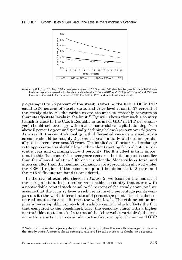
ployee equal to 28 percent of the steady state (i.e. the EU), GDP in PPPequal to 50 percent of steady state, and price level equal to 57 percent ofthe steady state. All the variables are assumed to smoothly converge totheir steady-state levels in the limit.11 Figure 1 shows that such a country(which is close to the Czech Republic in terms of GDP in PPP per emplo-yee) should achieve a growth rate of nontradable capital starting from above 5 percent a year and gradually declining below 3 percent over 25 years.As a result, the country’s real growth differential vis-à-vis a steady-stateeconomy should be roughly 2 percent a year initially, and decline gradu-ally to 1 percent over next 25 years. The implied equilibrium real exchangerate appreciation is slightly lower than that (starting from about 1.5 per-cent a year and declining below 1 percent). The B-S effect is thus impor-tant in this “benchmark” convergence scenario, but its impact is smallerthan the allowed inflation differential under the Maastricht criteria, andmuch smaller than the nominal exchange rate appreciation allowed underthe ERM II regime, if the membership in it is minimised to 2 years andthe �15 % fluctuation band is considered.

In the second example, shown in Figure 2, we focus on the impact ofthe risk premium. In particular, we consider a country that starts witha nontradable capital stock equal to 23 percent of the steady state, and weassume that the country faces a risk premium of 3 percentage points com-pared with the world interest rate of 6 percentage points (i.e., the domes-tic real interest rate is 1.5-times the world level). The risk premium im-plies a lower equilibrium stock of tradable capital, which offsets the factthat compared to the benchmark case, the economy starts with a highernontradable capital stock. In terms of the “observable variables”, the eco-nomy thus starts at values similar to the first example: the nominal GDP


FIGURE 1 Growth Rates of GDP and Price Level in the “Benchmark Scenario”

Note: �=�=0.4; �=�=0.1; 1–�=0.60; convergence speed = 2.7 % a year. h/h* denotes the growth differential of non-tradable capital compared with the steady state level. GDPnom/GDPnom*, GDPppp/GDPppp* and P/P* arethe same differentials for the nominal GDP, the GDP in PPP, and price level, respectively.

0 %

1 %

2 %

3 %

4 %

5 %

6 %

Yea

r-o

n-y

ear

gro

wth

rat

e

Time (in years)1 3 5 7 9 11 13 15 17 19 21 23 25

h/h* GDPnom/GDPnom* GDPppp/GDPppp* P/P*

11 Note that the model is purely deterministic, which implies the smooth convergence towardsthe steady state. A more realistic setting would need to take stochastic shocks into account.

per employee reaches roughly 28 percent of the steady state, GDP in PPP50 percent of steady state (close to the Czech starting point) and price le-vel 57 percent of the steady state. After the initial period, the risk pre-mium starts declining by 15 percent each year, converging gradually to-wards zero. Figure 2 shows that very little convergence takes place inthe starting period. The economy’s output is far from the EU levels; how-ever, given the risk premium, it is not very far from its conditional steadystate. Once the risk premium starts to decline, through, the GDP growthboth in nominal terms and in the PPP, as well as the price level conver-gence speed up immediately, in line with (11), (12), and (23). Moreover,this primary effect is further magnified by the fact that the reduced equ-ilibrium real interest rate creates an additional motivation for nontra-dable capital accumulation, which gradually starts to gain momentum.As a result, the real GDP growth differential increases above 2 percen-tage points, and only gradually declines towards 1 percentage point.The real exchange rate appreciation goes up to 2 percentage points initi-ally, and gradually decreases below 1 percentage point. The results arethus similar to the “benchmark” scenario of Figure 1, even though the maindriving force is different. The contribution of this alternative simulationconsists in illustrating the links between the risk premium, GDP growth,and real exchange rate appreciation, which are usually the key equilib-rium variables entering the forecasting process at the central bank – seee.g. (Bene‰ et al., 2002).

4. Demand Side of the Economy and the Speed of Convergence

In section 3, we focused on the supply side of the economy only. In par-ticular, we assumed that the speed of convergence was constant (which isbroadly consistent with the results of cross-country regressions by Barro


FIGURE 2 Impact of Declining Risk Premium

Note: �=�=0.4; �=�=0.1; 1–�=0.60; convergence speed 2.7 % a year. h/h* denotes the growth differential of nontrad-able capital compared with the steady state level. GDPnom/GDPnom*, GDPppp/GDPppp* and P/P* arethe same differentials for the nominal GDP, the GDP in PPP, and price level, respectively.

1 3 5 7 9 11 13 15 17 19 21 23 25

Yea

r-o

n-y

ear

gro

wth

rat

e

Time (in years)

h/h* GDPnom/GDPnom* GDPppp/GDPppp* P/P*

4.5 %

4.0 %

3.5 %

3.0 %

2.5 %

2.0 %

1.5 %

1.0 %

0.5 %

0.0 %

(1991) and others), and the allocation of labour across economic sectorswas fixed for each economy. In this section, we provide a deeper look intohow the above two factors are determined by the consumers’ behaviour ininteraction with the production and accumulation of nontradable capital.The discussion in this section is based on the Ramsey model in an openeconomy with nontradable (“human”) capital (Cohen – Sachs, 1986), (Barro– Sala-i-Martin, 1995), extended for the distinction between tradable andnontradable goods – e.g. (Obstfeld – Rogoff, 1996).

Let us adopt several assumptions to make the analysis easier to pre-sent. First, we assume that preferences between tradable and nontrad-able goods have a Cobb-Douglas (C-D) form, implying unitary elasticityof substitution between them – see e.g. (Obstfeld – Rogoff, 1996, pp. 222).Second, we assume that while one unit of tradable capital is equivalentto one unit of tradable good, in order to produce a unit of nontradable ca-pital, one needs to give up one unit of the consumption basket C (seethe definition in (14)).12 Third, we assume that the borrowing constraintis binding for a converging economy, implying that the sum of tradablecapital and foreign borrowing is zero, and the net assets of the economyare thus equal to the nontradable capital only. This allows us to formu-late the optimisation problem of a representative consumer in time s asfollows:


� 1t–s (Ct)1– – 1

max Us = �–––––� u(Ct), u(ct) = –––––––––,ct t=s 1 + � 1–

Ct = (cT,t)� (cN,t)1–�, > 0

s.t. Pt (Ht+1 – Ht) = wt – (cT,t + pN,t cN,t) + r~tPtHt

(14)

where cT,t is the consumption of tradable goods in time t, cN,t is consump-tion of nontradable goods in the same period, is the coefficient of relativerisk aversion, � is the subjective discount rate, and r~t is the market returnon renting nontradable capital in time t (which is in equilibrium equal toits marginal product). Pt, defined in (10), is the optimal price index forthe C-D utility function. Similarly to section 3, Ht, and wt denote the levelof the nontradable capital and the wage level, respectively.

The above specification of the utility function implies that the demandfunctions for tradable and nontradable goods are given by – see e.g. (Obst-feld – Rogoff, 1996):

12 The assumption that the production of the nontradable capital requires nontradable goodsfits quite well with the assumption that the nontradable capital cannot move across borders.The assumption is also convenient, for two reasons. First, the price of the nontradable capitaldevelops in the same way as the price of the consumer basket, which means that we do not haveto take into account relative price changes of the nontradable capital in the Euler equation (17).Second, the assumption means that the employment distribution between the tradable and non-tradable sectors is constant (see below). A more general assumption would be that the non-tradable capital is produced as a C-D combination of the tradable and nontradable good, with weights �H and (1–�H), respectively. Here we restrict our attention to the case of �H = �. Notethat in this respect we differ from the earlier dependent-economy literature, which assumedthat the nontradable capital is identical with the nontradable good (Brock – Turnovsky, 1994),(Turnovsky, 1997), i. e. another special case with �H = 0.

PtcT,t = �PtCt; cN,t = (1–�) ––––– Ct (15)pN,t

Note that the C-D utility function leads to constant nominal shares oftradable and nontradable goods in consumer expenditures in equilibrium.This allows us to rewrite the flow budget constraint of equation (14) as:

wt(Ht+1 – Ht) = –– – Ct + r~tHt (16)Pt

which is similar to the budget constraint of a representative agent in an eco-nomy without the distinction between tradable and nontradable goods.

When we maximise the utility function of equation (14) subject to (16),we get a standard optimality condition (“Euler equation”):

Ct+1 1+r~t

1

–––– = �––––�––

(17)Ct 1+�

If we assume away depreciation of the nontradable capital, the returnon the nontradable capital should be equal to its marginal product (deno-ted fh,t) in equilibrium. Thanks to the assumption of perfect mobility ofthe nontradable capital – and thus equality of its marginal product – be-tween sectors, we can concentrate on the marginal product of the nontrad-able capital in the tradable sector only. Using our previous results fromequations (5), (6), and (7), this marginal product can be expressed as:13


h–

tZt ε–1 h

–tZt

ε–1

fh,t = �BT,t �––––� = ε (1 – a) BT,t �––––��E,t �E,t

� �BT,t � (AT,t) �–––––� ; ε � –––

rt*+ � 1–�

�––––1–�

1––––1–�

(18)

Equations (17) and (18) together with the standard transversality con-dition14 describe the consumption and investment behaviour in the model.

To close the model, we need to find a general equilibrium in which de-

13 Note that this is the derivative of production per employee in tradable sector, which is given by

YT h–

Zε

� �––– = BT �––�; BT � (AT) �––––––� ; ε � ––––, with respect to tradable capital, mul-LT � r* + � 1 – �

tiplied by (1–�). The term �Bh–ε that we effectively deduct from the reduced-form production

function equals to the flow of rents from the tradable capital abroad.

1–––– 1–�

�–––– 1–�

mand equals supply in both the tradable and the nontradable sector. In other words, we are looking for a situation in which

cT,t + IT,t = (1–�) YT,t; cN,t + IN,t = YN,t (19)

where IT,t is the amount of tradable goods used for investment into non-tradable capital in time t and IN,t is the volume of nontradable goods in-vested in nontradable capital. Note that the first equation reflects the factthat a fraction � of the tradable production goes as a reward to tradablecapital, which is fully foreign-owned in equilibrium.

The assumption that nontradable capital is a C-D combination of the trad-able and nontradable goods helps to simplify the computations, as it means that it is optimal to use the inputs into the investment process sothat:

�IT,t = ––––– pN,t IN,t (20)

1 – �

which is analogous to equation (15).15 Combining equations (15), (19), and(20) with the expressions for the tradable production and the nominal va-lue of nontradable production, which we had to derive already when ex-pressing the nominal GDP in equation (12) of section 3, we find that the equi-librium requires the following equality:

1–�–��E = –––––––––––––––––––– (21)

(1–�–�) + (1–�)(1–�–�)

This means that in the equilibrium of this simplified version of the mo-del, the labour shares of the tradable and nontradable sectors are con-stant, determined by the technological parameters. As a result, the pricelevel, nominal GDP, and real GDP are functions of the per-capita nontra-dable capital only (plus the risk premium; see section 3), which makesthe analysis of the convergence process much easier. Note that with the va-lues of technological coefficients used in Figures 1 and 2 (i.e. �=�=0.4;�=�=0.1), the labour share of the tradable sector would be about 30 per-cent. This is roughly the same as the median share of agriculture and ma-nufacturing on employment in the sample of countries in (âihák – Holub,2003), increasing our confidence that these calibrations are not unrealis-tic.16

We can use our results to discuss the process of real and price conver-gence in the model. Convergence in the standard closed-economy (Ramsey)


14 The transversality condition says that the present value of households’ assets must ap-proach 0 as time goes to infinity. It can be written as

1t

lim �H(t) �–––––––� � = 0, where t is time, and R(t) is the interest rate between now and time t.

t→�1 + R(t)

15 Note that in the more general case, � would be replaced with �H in this equation.

growth model can be described by the equation log[y(t)] = e–Bt log[y(0)] ++ (1–e–Bt) log(y*), where B>0. The logarithm of output per unit of effectivelabour is therefore a weighted average of the initial value and the steady--state value, with the weight of the initial value declining exponentiallywith time. The speed of convergence, B, depends on parameters determi-ning technology and preferences. For the C-D function:

1 – �~ �+�+g2B = � 2 + 4 �––––�(�+�+g)�–––––– – (n+g+�)��1/2

– (22) �~

where is defined as = � – n – (1–)g>0 and �~ denotes the capital-in-tensity coefficient for a single-good closed economy.17 In our open economyversion of the model, however, we have to replace �~ in equation (22) withε � �/(1–�), as defined in equation (18).

For usual values of the other parameters,18 the speed of convergence isfrom 1.5 percent per year (for �/�=0) to about 3 percent per year (for �/�=1)and further to for instance 5 percent (for �/�=3).19 If we assume that lessthan a half of total capital in the production of tradable goods is tradable(i.e., �/��1), then the predicted speed of convergence would be in the rangeof 1.5–3.0 percent, which is consistent with most empirical studies (Barro– Sala-i-Martin, 1995). Note that the calibration used in Figure 1 wouldimply a convergence speed close to the upper end of this interval. We usedsuch a convergence speed (in particular, 2.7 percent a year) in the conver-gence scenarios of section 3.


16 In reality, the share of employment in tradable sector tends to be lower for richer count-ries. For example, in (âihák – Holub, 2003), we found a significantly negative relationshipbetween employment in agriculture and manufacturing and the log of GDP in PPP. The abovemodel explains this tendency by the fact that the indebted converging countries have to al-locate more labour to the tradable sector to be able to service their borrowing of tradable ca-pital (see the term (1–�) in the denominator of (21)). A related – but more general – expla-nation is that rich countries can import more tradable goods from abroad with smallerdomestic tradable sectors (we thank for this remark to an anonymous referee). This can beeither due to their net creditor position (financing additional imports by interest incomes –see above) or more appreciated exchange rates, resulting for example from better terms oftrade. The latter factor, however, goes beyond the scope of this section, which builds on the Ba-lassa-Samuelson model with its simplifying assumptions. Another way to introduce the ob-served tendency would be to assume that �H>� in the production of nontradable capital, mea-ning that a converging country would have to allocate more labour to the production oftradables.17 Where � denotes capital depreciation, n population growth, and g exogenous technological pro-gress. We have so far ignored these factors for simplicity, but their introduction would be straight-forward.18 The usual values of the parameters are �=1/3, n=1 percent, g=2 percent, and �=3 percent. Asregards the parameters of impatience, “reasonable” values include � of about 0.02 and lowerthan 10 (Barro – Sala-i-Martin, 1995).19 For �=0, all capital in the economy would be tradable, so that the economy would effectivelyreturn to the case of an open economy with perfect capital mobility. Indeed, �=0 means ε=0, andthe convergence coefficient, B, is infinitely high. The case of �=0, on the contrary, would cor-respond to a closed economy, because there is no tradable capital. In this case, ε��, and the con-vergence coefficient is the same as in the case of a closed economy.

5. Balassa-Samuelson Model with More than Two Goods

One of the problems of the standard B-S approach is that the distinctionbetween tradable and nontradable goods is largely artificial. In empiricalcross-country comparisons, each commodity group generally behaves asa blend of tradable and nontradable elements rather than purely tradableor purely nontradable – see (âihák – Holub, 2003).

To introduce such a variety of goods into the model, let us assume thatthere are x consumption goods, produced by combining tradable and non-tradable goods – which, in turn, are subject to the production process de-scribed in the B-S model of section 3. In contrast to the standard B-Smodel, the tradable and nontradable goods are not consumed directly, butrather serve as intermediate inputs into the production of consumption (re-tail) goods. For simplicity and brevity, we limit ourselves to the case inwhich the shares of tradable and nontradable inputs are fixed, discussingonly informally the implications of substitutability between these two in-puts (more formal discussion is in (Holub – âihák, 2003)).

Let us thus assume that consumption good i is produced according tothe following formula:

Ti,t Ni,tyi,t = min �–––, ––––––�; 0 < wi < 1 (23)wi 1 – wi

where yi,t is output of the good i (=1, 2, ... x) at time t, Ti,t is the tradableinput , Ni,t is the nontradable input, and wi is the weight of the tradableinput in the consumption good i. Equation (23) is a formalization of the ideathat each consumption good contains nontradable elements (such as trans-portation costs, wholesale margins, and retail margins) as well as trad-able elements (the part of the good after the adjustment for all the non-tradable elements).20

Profit maximization under this production function implies that the ra-tio of tradable and nontradable factors in optimum has to be wi/(1–wi).The marginal cost is then given by:

�(Ti + pN Ni)MCi = ––––––––––– = wi + pN (1–wi) (24)Ti

� ––wi

Assuming that the consumption goods markets are perfectly competi-tive, the price of the consumption good i, pi, would be equal to the margi-


20 In (âihák – Holub, 2003), we have attempted to proxy the “degree of nontradability” ofa commodity group by the slope coefficient in a cross-country regression between the com-modity group’s price and GDP. We have found that in the 30 commodity groups covered un-der private consumption in the 1999 ICP, the empirical degrees of nontradability ranged from10 to 85 percent. In other words, there was no purely tradable or purely nontradable com-modity group.

nal costs. This means that pi is a weighted average of the price of tradablegoods (normalized at 1) and the price of nontradable goods, the weights be-ing the shares of tradable and nontradable inputs, respectively. For a gi-ven price of nontradables, the price of a consumption good would be a li-near function of the weight of the tradable element, wi, increasing from pN

to 1 for pN<1 and decreasing from pN to 1 for pN>1 (Figure 3a).An increase in pN would increase the price of each individual consump-

tion good, pi, thereby raising the aggregate price level. The increase willbe the higher the less tradable the good, since �pi /�pN = 1 – wi . For pN�1,an increase in pN would increase the overall dispersion of the individualprices, while for pN<1, it would decrease the price dispersion. To see this,we can consider two goods (i and j) with different degrees of tradability.The impact of a change in pN on the difference of the prices of these goodscorresponds to the difference in the weights of nontradable inputs in thesetwo goods, namely:

� (pi – pj) � [wi – wj + pN (wj – wi)]–––––––– = –––––––––––––––––––– = wj – wi� pN � pN (25)

Let us take a good i that is less tradable than a good j, that is, wi< wj.Equation (25) implies that an increase in pN always increases the price ofthe good i more than it increases the price of the good j, because of its high-er share of the nontradable element. For pN�1, it holds from (24) thatpi�pj, so the increase in (pi–pj) as a result of the increasing pN meansan increase in the differences between the two prices. For pN<1, it holdsfrom (24) that pi<pj, so the increase in (pi–pj) as a result of the increa-sing pN means a decrease in the differences between the two prices. Fi-gure 3b illustrates this conclusion, showing the relationship betweenthe price level (P), defined as the weighted average of individual prices,and the price dispersion (�), defined as a weighted standard deviation ofthe individual prices, with the weights corresponding to the shares of


FIGURE 3 Prices, Price Levels, and Price Dispersion with More than Two Goods

(a) Price vs. tradability (b) Price level vs. price dispersion

pN1>1pN2=1pN3<1

0 0.5 1

1

pN1

pN3

Pi

w0 0.1 0.2 0.3 0.4 0.5

2.0

1.5

1.0

0.5

0.0

P

�

the individual goods in the overall consumption. The relationship betweenP and � is negative for low price levels (P<1) and positive for high pricelevels (P>1).21

An alternative to assuming fixed shares of tradable and nontradable fac-tors (as in (23)) would be to assume that they are, to some extent, substi-tutable. We study such a case in (Holub – âihák, 2003), and find that the re-lationship between the price level (P) and the price dispersion (�) remainsnegative for lower price levels and positive for higher price levels; however,thanks to the substitutability between the inputs, the negatively slopingportion is longer and the transition from a negative slope to a positive oneis a gradual one. This theoretical conclusion is consistent with the findingsof a series of our empirical papers on relative prices and price levels (Ho-lub – âihák, 2000), (âihák – Holub, 2001a,b, 2003). In these papers, wehave found out that for a pooled sample of EU countries and CEE transi-tion countries, there is a significant negative relationship between the de-gree of deviations of relative prices in a given country vis-à-vis the systemof relative prices in the reference country and the price level.22 We havealso found that the relationship is still negative, but less so, if we look onlyat EU countries, and that the relationship is very weak when applied toa world-wide sample of countries.

As a further generalisation, we could assume that producers in some (orall) markets face a downward sloping demand function and are able to settheir price above marginal costs, depending on the price elasticity of de-mand. Again, we report the results in detail in (Holub – âihák, 2003).The implications of this case depend on whether the differences in demandelasticities have any systematic pattern or not. As regards the relation-ship between the price level (P) and the price dispersion (�), though, the in-troduction of imperfect competition would not change the basic conclusionthat for lower price levels, the relationship tends to be negative, while forhigher price levels, it tends to be positive, even though both the price le-vel and the price dispersion would tend to be higher under imperfect com-petition than under perfect competition.

The introduction of imperfect competition brings additional insightsby allowing us to study, for example, the impact of a systematic rela-tionship between the price of nontradables in a country, and the priceelasticities, which is indeed consistent with empirical evidence. In par-ticular, we could assume that the elasticity of demand for the same


21 To plot this curve, we have generated 10,000 consumption goods with the wis drawn froma uniform distribution over the interval (0,1).22 The degree of deviations of relative prices was measured as a weighted standard deviation ofcomparable price levels of individual goods in the given country relative to the average compa-rable price level,

1_____________

� = –– �wi (Pi – �)2, where wi are weights of the individual goods in the consumption bas-�

i

ket and � is the average price level of consumption. This is consistent with the definition ofthe price dispersion in the theoretical calculations in Figure 3b. The only difference is thatthe empirical comparable price levels are measured as ratios to the same prices in a referencecountry, whilst here we measure all prices in terms of a single theoretical numeraire, i.e. the priceof tradable input.

good differs in individual countries and that companies are – due totheir monopolistic power – able to set different prices in different count-ries.23 As a result, the price of the same good would be higher inthe countries with a less elastic demand. Demand functions are likelyto be less elastic in more advanced countries (i.e., countries with high-er prices of nontradables), as higher income levels enable consumersto put more emphasis on non-price factors such as the brand or the per-ceived quality of the good. This effect would tend to decrease the mea-sured price dispersion for countries with low price levels (and high priceelasticity of demand), while increasing it for countries with high pricelevels (and low elasticity of demand). However, there are also factorsattenuating this effect, in particular the fact that goods exported fromless developed countries to developed countries tend to face a more elas-tic demand function, because of their perception as being “inferior”. In(âihák – Holub, 2001a,b; 2003) we have indeed found empirical evi-dence supporting the existence of such effects for the case of EU andCEE countries.

Finally, cross-country price differences may be also influenced by go-vernment policies such as the competition policy and taxation, which mayinfluence the mark-ups over marginal costs. As a result, a part of the priceconvergence process may be related to all these additional effects descri-bed in this section, rather than to the B-S effect associated with the chan-ging relative price of the tradable and nontradable inputs.

6. Conclusion

In this article, we provided a theoretical reference point for the discus-sions on adjustments in the price level and relative prices. We presenteda model integrating the Balassa-Samuelson model of real equilibrium ex-change rate with a model of accumulation of capital consistent withthe new growth literature, and with the demand side of the economy. Wehave also shown how the model can be generalized to a case of more thantwo goods.

The presented extensions to the B-S model provide several useful in-sights into the likely price adjustment process in the Central Europeaneconomies. For instance, the simulations based on the model with nontrad-able capital, presented in this article, allow to assess in a consistent fra-mework the links between the risk premium, GDP growth, and real ex-change appreciation, which are typically the key equilibrium variables inthe macroeconomic forecasting process.

The extension of the model to the case of more than two goods also pro-vided intriguing insights into the nature of the relative price adjustmentprocess. The calculations suggest that for countries with relatively low price


23 In a review of the literature, it appears that the car industry is particularly affected by pricediscrimination. For example, Verboven (1996) finds that European car markets are segmented,with producers gaining higher markups in their home country than in export destination count-ries.

levels, there should be a negative relationship between the price disper-sion and price levels; the relationship should become less negative for count-ries with higher price level, and eventually turn positive with increa-sing price levels. This prediction is consistent with empirical findings ba-sed on data for CEE and EU countries.

REFERENCES

ASEA, P. K. – CORDEN, W. M. (1994): The Balassa-Samuelson Model: An Overview. Review ofInternational Economics, 1994, no. 2 (October), pp. 191–200.

ASEA, P. K. – MENDOZA, E. (1994): The Balassa-Samuelson Model: A General-EquilibriumAppraisal. Review of International Economics; 1994, no. 2 (October), pp. 244–267.

BALASSA, B. (1964): The Purchasing Power Parity Doctrine: A Reappraisal. Journal of Politi-cal Economy, vol. 72, 1964, pp. 584–96.

BARRO, R. J. (1991): Economic Growth in a Cross Section of Countries. Quarterly Journal ofEconomics, vol. 106, 1991, no. 2 (May), pp. 407–443.

BARRO, R. J. – SALA-I-MARTIN, X. (1995): Economic Growth. New York, McGraw-Hill, 1995.

BENE·, J. – VÁVRA, D. – VLâEK, J. (2002): Stfiednûdobá makroekonomická predikce, makro-ekonomické modely v analytickém systému âNB. Finance a úvûr, roã. 52, 2002, ã. 4, ss. 197–231.

BROCK, P. L. – TURNOVSKY, S. J. (1994): The Dependent-Economy Model with Both Tradedand Nontraded Capital Goods. Review of International Economics, 1994, no. 2 (October),pp. 306–325.

BRUNO, M. (1982): Adjustment and Structural Change under Supply Shocks. ScandinavianJournal of Economics, vol. 84, 1982, pp. 199–221.

COHEN, D. – SACHS. J. (1986): Growth and External Debt under Risk of Debt Repudiation.European Economic Review, vol. 30, no. 3 (June), pp. 526–560.

âIHÁK, M. – HOLUB, T. (2001a): Convergence of Relative Prices and Inflation in the CEECountries. Washington, D. C., International Monetary Fund, Working Paper, no. 01/124.

âIHÁK, M. – HOLUB, T. (2001b): Cenová konvergence k EU – pár nezodpovûzen˘ch otázek. Fi-nance a úvûr, roã. 51, 2001, ã. 5, ss. 331–349.

âIHÁK, M. – HOLUB, T. (2003): Price Convergence to the EU: What Do the 1999 ICP Data TellUs? Prague, Czech National Bank, Working Paper, no. 2/2003.

DICKENS, W. – KATZ, L. (1987): Inter-industry Wage Differences and Industry Characteris-tics. In: Lang, K. – Leonard, J. S. (eds.): Unemployment and the Structure of Labor Markets.New York and Oxford, Blackwell, pp. 48–89.

FISCHER, S. – FRENKEL, J. (1972): Investment, the Two-Sector Model and Trade in Debt andCapital Goods. Journal of International Economics, 1972, no. 2, pp. 211–33.

FRENKEL, J. – MUSSA, M. (1986): Asset Markets, Exchange Rates, and the Balance of Pay-ments. In: Grossman, E. – Rogoff, K. (eds): Handbook of International Economics. Vol. 3. Amster-dam, North Holland, 1986, Chapter 14.

HELWEGE, J. (1992): Sectoral Shifts and Interindustry Wage Differentials. Journal of LaborEconomics, vol. 10, 1992, no. 1 (January), pp. 55–84.

HARROD, R. (1933): International Economics. London, James Nisbet and Cambridge Univer-sity Press, 1933.

HESTON, A. – LIPSEY, R. E. (eds.) (1999): International and Interarea Comparisons of Income,Output and Prices. Studies in Income and Wealth, vol. 61, NBER (Chicago, The University ofChicago Press).

HOLUB, T. – âIHÁK, M. (2000): Cenová konvergence k EU – problém relativních cen. Politickáekonomie, 2000, ã. 5, ss. 660–671.

HOLUB, T. – âIHÁK, M. (2003): Price Convergence: What Can the Balassa-Samuelson ModelTell Us? Prague, Czech National Bank, Working Paper (forthcoming).


KRAVIS, I. B. – HESTON, A. – SUMMERS, R. (1982): World Product and Income: Internatio-nal Comparisons of Real Gross Product. Baltimore, The Johns Hopkins University Press andthe World Bank, 1982.

KREIDL, V. (1997): RovnováÏn˘ mûnov˘ kurz. Finance a úvûr, roã. 47, 1997, ã. 10, ss. 580–97.

MUSSA, M. (1984): The Theory of Exchange Rate Determination. In: Bilson, J. F. O. – Mars-ton, R. C. (eds): Exchange Rate Theory and Practice, NBER Conference Report, Chicago, Chi-cago University Press, 1984.

NEAL, D. (1995): Industry-Specific Human Capital: Evidence from Displaced Workers. Journalof Labor Economics, vol. 13, 1995, no. 4 (October), pp. 653–77.

NEARY, J. P. – PURVIS, D. D. (1982): Sectoral Shocks in a Dependent Economy: Long-run Ad-justment and Short-run Adjustment. Scandinavian Journal of Economics, vol. 84, 1982,pp. 229–53.

OBSTFELD, M. – ROGOFF, K. (1996): Foundations of International Macroeconomics. Cam-bridge, MA, MIT Press, 1996.

SALTER, W. E. G. (1959): Internal and External Balance: The Role of Price and ExpenditureEffects. Economic Record, vol. 35, 1959, pp. 226–38.

SAMUELSON, P. A. (1964): Theoretical Notes on Trade Problems. Review of Economics and Sta-tistics, vol. 46 (May), 1964, pp. 145–154.

SAMUELSON, P. A. (1994): Facets of Balassa-Samuelson Thirty Years Later. Review of Inter-national Economics, 1994, no. 2 (October), pp. 191–325.

STRAUSS, J. (1998): Relative Price Determination in the Medium Run: The Influence of Wa-ges, Productivity, and International Prices. Southern Economic Journal, vol. 65, 1998, no. 2 (Oc-tober), pp. 223–44.

SVENSSON, L. E. O. (1982): Comment on M. Bruno, ‘Adjustment and Structural Change un-der Supply Shocks’. Scandinavian Journal of Economics, vol. 84, 1982, pp. 223–27.

SWAN, T. W. (1960): Economic Control in a Dependent Economy. Economic Record, vol. 36, 1960,pp. 51–66.

TURNOVSKY, S. J. (1997): International Macroeconomic Dynamics. Cambridge, MA, The MITPress, 1997.

VERBOVEN, F. (1996): International Price Discrimination in the European Car Market. RANDJournal of Economics, vol. 27, 1996, pp. 240–268.


SUMMARY

JEL Classification: E31, E52, E58, F15, P22Keywords: inflation – relative prices – Balassa-Samuelson model

Price Convergence: What Can the Balassa-Samuelson Model Tell Us?Tomáš HOLUB – Czech National Bank ([email protected])Martin ČIHÁK – International Monetary Fund ([email protected])

The article contributes to the theory of convergence in the price level and relativeprices. The authors present a model integrating the Balassa-Samuelson model ofreal equilibrium exchange rate with a model of capital accumulation and with thedemand side of the economy. They also show how the Balassa-Samuelson model canbe extended to the case of more than two goods. The predictions of the Balassa-Sa-muelson model are generally consistent with empirical findings in Central and Eas-tern European countries. The authors show how the model can be used toward pro-jecting price convergence in a transition economy.


price convergence: what can the balassa-samuelson model...

Documents