The Harrod-Balassa-Samuelson Effect:

Reconciling the Evidence

ECB -BoC Workshop : “Exchange Rates and Macroeconomic Adjustment”

15 -16 June 2011

Christiane BaumeisterEhsan U. Choudhri

Lawrence Schembri

This presentation represents the views of the authors, not the Bank of Canada

Introduction & Motivation: HBS Hypothesis

Developed by Harrod (1933), Balassa (1964) and Samuelson (1964)

To explain sustained real exchange rate (RER) appreciations in rapidly

growing economies, via productivity increases

– Strongest evidence in Japan and Eastern Europe

Posits that relatively strong productivity growth in the tradables sector

raises the relative price of nontradables and the RER

Provides an argument against long-run purchasing power parity

2

Japan: RER and Real Per Capita Income

100

125

150

175

200

225

250

275

1970

1971

1972

1973

1974

1975

1976

1977

1978

1979

1980

1981

1982

1983

1984

1985

1986

1987

1988

1989

1990

1991

1992

1993

1994

1995

1996

1997

1998

1999

2000

2001

2002

2003

2004

2005

2006

2007

2008

2009

(1970 = 100)

REER index Real GDP per capita index3

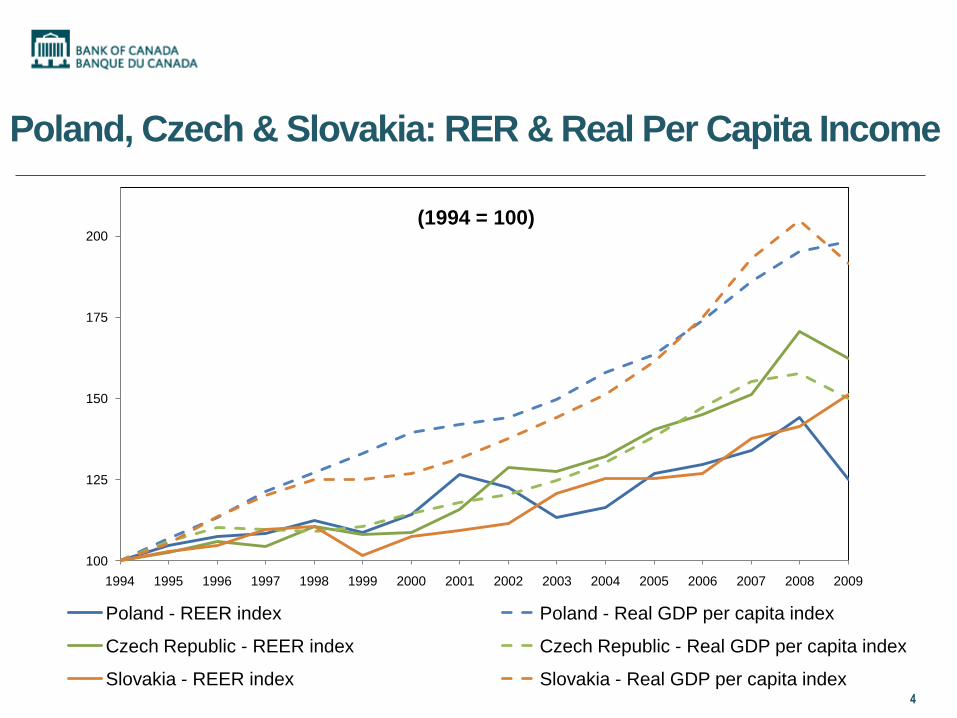
Poland, Czech & Slovakia: RER & Real Per Capita Income

100

125

150

175

200

1994 1995 1996 1997 1998 1999 2000 2001 2002 2003 2004 2005 2006 2007 2008 2009

(1994 = 100)

Poland - REER index Poland - Real GDP per capita index

Czech Republic - REER index Czech Republic - Real GDP per capita index

Slovakia - REER index Slovakia - Real GDP per capita index4

Brazil, Chile and Mexico: RER & Per Capita Income

60

80

100

120

140

160

180

1994 1995 1996 1997 1998 1999 2000 2001 2002 2003 2004 2005 2006 2007 2008 2009

(1994 = 100)

Brazil - REER index Brazil - Real GDP per capita index

Chile - REER index Chile - Real GDP per capita index

Mexico - REER index Mexico - Real GDP per capita index 5

RER adjustment in Latin America versus East Asia

6

1990 1995 2000 2005 2010

0

20

40

60

80

100

120

140

160

1990 = 100

Latin America East Asia

REER

Source: JP Morgan

Chart 2: EME Real Effective Exchange Rate

Purpose: Reconciling the evidence

The main purpose of the paper is to attempt to reconcile the mixed evidence surrounding the HBS hypothesis

Both theoretically and empirically

Derive a theoretically based empirical model

– Using per-capita income is not a true test of HBS hypothesis

Estimate the model using a consistent OECD panel database on labour productivity by sector

7

Methodology / Outline

1. Derive the conventional empirical model for the HBS hypothesis

2. Derive an extended version of the empirical model of the HBS hypothesis using a monopolistically competitive model

3. Estimate the empirical model using time series/panel data techniques

4. Interpret and reconcile the results

8

Theoretical Framework

Derive the empirical relations to represent the HBS hypothesis

Two countries (home and foreign), one factor (labour), and two composite goods (tradable and nontradable goods)

Focus on long-run effects: Assume flexible prices, financial autarky, mobile labour and balanced trade

To facilitate comparison across two models, assume CES aggregators and a continuum of goods in tradable and nontradable bundles

9

The Conventional Model

Consumption: Aggregate, Nontradable and Tradable

Production: Nontradable and Tradable

10

/( 1)1/ ( 1)/ 1/ ( 1)/

/( 1)( 1/

/( 1)( 1/

(1 )

( )

( )

N

T

N T

N Ni

T Tj

C C C

C C i di

C C j dj

( ) ( )

( ) ( )

N N N

T T T

Y i A L i

Y j A L j

The Conventional Model

Real Exchange Rate Relation:

Each country’s tradable/nontradable productivity ratio affects the RER

via the relative price of nontradables

Assume that the share of nontradables is same across countries, the

RER is related to home/foreign productivity ratio in each sector

Letting a hat over a variable denote the log deviation from its initial

value, obtain a typical form of the HBS relation:

11

* *ˆ ˆ ˆ ˆ ˆ( ) ( )T T N NQ A A A A * *

Monopolistic Competition Model

12

Monopolistic competition in each sector with symmetrical firms and

free entry

Nontradable good is still an aggregate of (nontradable) varieties

Tradable good now is of a continuum of home & foreign varieties:

*

/( 1)1/ ( 1)/ 1/ ( 1)/

/( 1) /( 1)( 1)/ * ( 1)/ *

(1 ) ,

( ) , ( )H F

T H F

H H F Fj j

C C C

C C j dj C C j dj

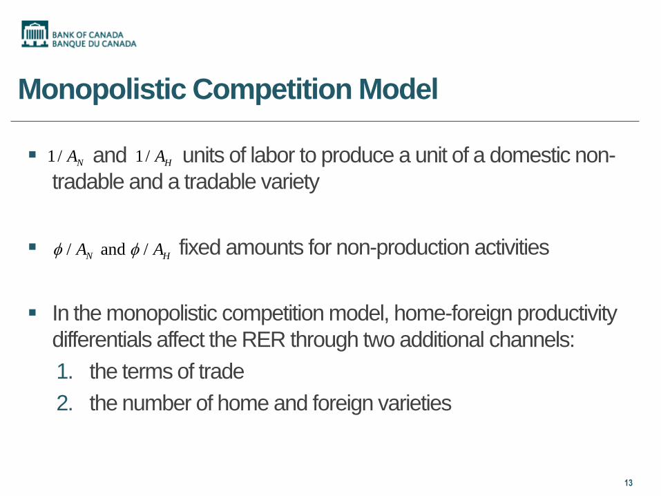
Monopolistic Competition Model

13

and units of labor to produce a unit of a domestic non-

tradable and a tradable variety

fixed amounts for non-production activities

In the monopolistic competition model, home-foreign productivity

differentials affect the RER through two additional channels:

1. the terms of trade

2. the number of home and foreign varieties

1/ NA 1/ HA

/ and /N HA A

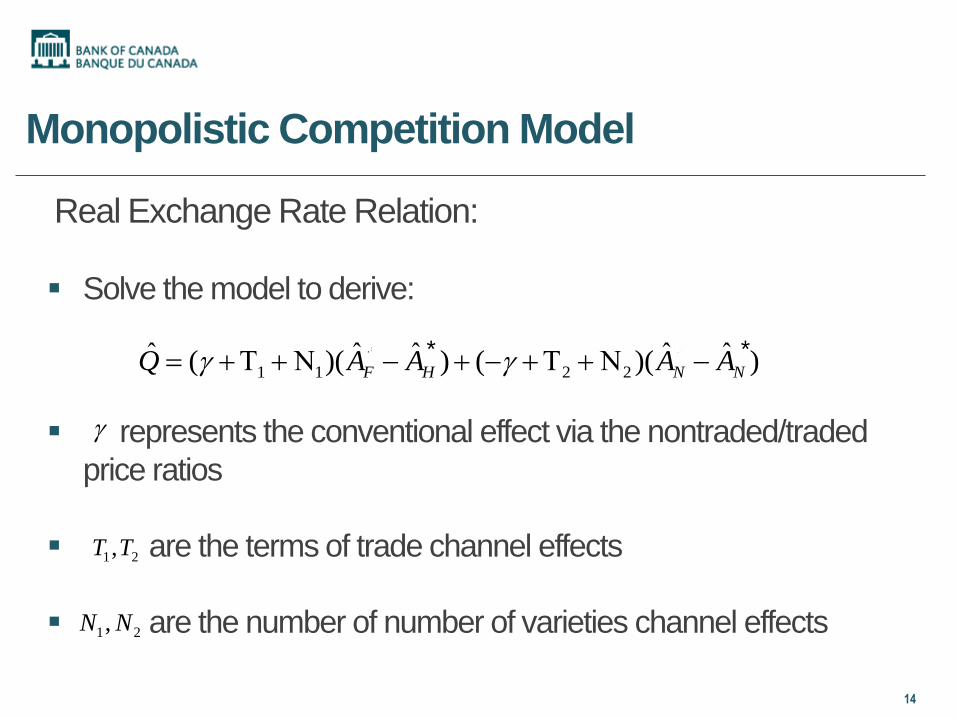
Monopolistic Competition Model

Real Exchange Rate Relation:

Solve the model to derive:

represents the conventional effect via the nontraded/traded

price ratios

are the terms of trade channel effects

are the number of number of varieties channel effects

14

1 2,T T

1 2,N N

* *

1 1 2 2ˆ ˆ ˆ ˆ ˆ( )( ) ( )( )F H N NQ A A A A * *

The Terms of Trade Channel

The effects through the terms of trade channel depend on:

1. ε - elasticity of substitution between tradables & nontradables

2. η - elasticity of substitution between home & foreign tradables

3. θ – θ* - home bias in the consumption of tradable goods

The effects via the number of varieties channel also depends on

the same parameters

15

Data

Annual data from 1977 to 2006 – 30 observations per country

16 OECD countries: Austria, Belgium, Canada, Denmark, Finland, France, Germany, Italy, Japan, Korea, the Netherlands, Norway, Portugal, Sweden, U.K. and U.S.

RER and productivity differential data are calculated relative to the average of the rest of the sample

RER is obtained using NER and CPI from the IMF’s IFS database

Labour productivity is output per employee in four tradable goods industries and five nontradable goods industries from the OECD’s STAN database

16

Regression model and estimation

Dynamic OLS specification (to incorporate co-integration)

ln Qi = δi +βiT(lnAiT - lnAwT) + βiN (lnAiN - lnAwN) + one lead and one lag of the first differences

HBS Hypothesis: βiT > 0 and βiN < 0

Three different panel DOLS techniques:

1. Fixed -Effect Panel: Homogeneous LR & SR coefficients

2. Pooled Mean-Group Panel: Homogeneous LR coefficients

3. Group Mean Panel: Panel average of heterogeneous LR coefficients

17

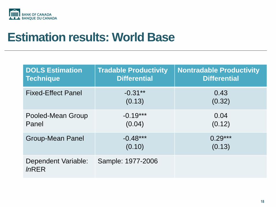
Estimation results: World Base

DOLS Estimation

Technique

Tradable Productivity

Differential

Nontradable Productivity

Differential

Fixed-Effect Panel -0.31**

(0.13)

0.43

(0.32)

Pooled-Mean Group

Panel

-0.19***

(0.04)

0.04

(0.12)

Group-Mean Panel -0.48***

(0.10)

0.29***

(0.13)

Dependent Variable:

lnRER

Sample: 1977-2006

18

Estimation Results: Other Notable Findings

Using the U.S. or Germany as the basis for comparison does not change the qualitative nature of the results

– Values/significance of the coefficients change somewhat

The results using aggregate productivity as the explanatory variable, as a proxy for per capita income, are more mixed

Estimates by country are very heterogeneous with no obvious pattern

19

Interpreting and Reconciling the Results

The mixed results are consistent with other findings

– E.g., Peltonen and Sager (ECB, 2009)

Theoretical reconciliation

– Numerically simulating the theoretical monopolistic competition model with different estimates for key substitution elasticities

Empirical reconciliation

– Investigate robustness of the results

20

Home-Foreign Goods Substitution Elasticity

The effect of the tradable productivity differential depends on η

– Below a critical value, the effects (via the terms of trade and

number of varieties channels) can cause a real depreciation

– The increase in home productivity causes an increase in supply

and a decline in the terms of trade

Thus, the conventional HBS effect can be offset and even

reversed for a small enough value of η

21

Tradable-Nontradable Substitution Elasticity

If ε > 1 the nontradable productivity differential causes a RER

appreciation via the terms of trade

– E.g., a productivity increase in home nontradables would raise the

share of nontradables and reduce the supply of tradables, thereby

increasing the terms of trade

The nontradable productivity differential could also cause a real

appreciation via the number of varieties

Thus, the sign of the coefficient of non-tradable productivity

differential in the conventional model could also be reversed

22

Reconciling the Results: Numerical Simulation

We use data for OECD countries (averaged over periods & countries) to

set the nontradable share equal to 0.73 and the home bias equal to 0.3.

We let the elasticity of substitution between varieties ( ζ ) equal to 6

based on the evidence on mark-ups ~ 20%

Estimates of the elasticity of substitution between home and foreign

tradable goods (η) range from <1 to >>1

Estimates of elasticity of substitution between tradable and non-tradable

goods (ε) has received less attention, but worth exploring

– Typically assumed to be close to one

23

Numerical simulation: Effects on lnQ (RER)

ε η ln ΑT – ln ΑT ln ΑN – ln ΑN

1.0 3.0 0.594 -0.801

1.0 1.0 -0.091 -0.802

1.0 0.5 -1.659 -0.803

2.0 3.0 0.532 -0.756

2.0 1.0 -0.227 -0375

2.0 0.5 -0925 0.009

3.0 3.0 0.476 -0.705

3.0 1.0 -0.300 -0.130

3.0 0.5 -0.733 0.219

24

* *

Empirical robustness

Consider different samples periods

Signs of estimated LR coefficients on the productivity

differentials are sensitive to the sample period

Lee and Tang (2007) also find that the results are sensitive to

the definition of productivity (TFP versus labour)

25

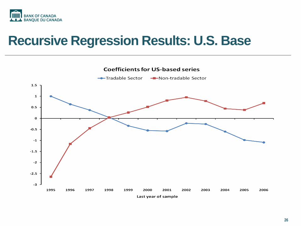
Recursive Regression Results: U.S. Base

26

Recursive Regression Results: World Base

27

Concluding remarks

Made progress in understanding mixed empirical results for HBS

hypothesis by extending theoretical model

Empirical results are unstable over time and across countries

– Sample may be too short to obtain low-frequency estimates

– Time series/panel techniques unable to remove cyclical effects and

other macro factors

Future work:

– Investigate the empirical results further (e.g., RER & China)

– Build a dynamic version of model to replicate mixed empirical results

28

Extra slides

29

The Terms of Trade Channel

The effects through the terms of trade adjustment are

The effects depend on:

– the elasticity of substitution between tradables & nontradables

– the elasticity of substitution between home & foreign tradables

– the home bias in the consumption of tradable goods

30

1

2

*

[ (1 ) ](1 )

( 1)

[ (1 ) ]( 1)

( 1)

1 (1 )(1 ) (1 )

( 1) / ( ),

The Number of Varieties Channel

The effects through the adjustment of number of varieties are

These effects also depend on the two elasticities and home

bias

31

1

2

(1 )1

1

( 1)1

1

Implications for the Productivity Effects

Adjustment in terms of trade can weaken or even reverse the effect

of the tradable productivity differential on RER via supply effects

– (Benigno and Thoenissen, 2003)

The effect through the number of varieties channel has not been fully

explored

The role of the two channels for the effect of the nontradable

productivity differential also needs to be examined

32

Home-Foreign Substitution Elasticity: Estimates

Controversy about the value of the elasticity of substitution

between home and foreign tradable goods

Estimates based on macro models indicate that the value of this

elasticity is low and below 1.0 (Bergin, 2006; Lubik and

Schorfheide, 2005)

Studies based on the disaggregated trade data suggest the

average value of the elasticity to be much larger (Imbs and

Mejean, 2009)

33

Tradable-Nontradable Substitution Elasticity: Estimates

Elasticity of substitution between tradable and non-tradable goods

has received less attention

– Typically assumed to be close to one

But this assumption is not based on empirical estimation, and this

elasticity could be greater than one

Given the uncertainty about the values of the two elasticities, we

consider a wide range of values for these elasticities

34