price dynamics for durable goods - home | princeton …itskhoki/papers/durablepricing_slides.pdf ·...
TRANSCRIPT

Price Dynamics for Durable Goods
Michal Fabinger Gita Gopinath Oleg ItskhokiHarvard Harvard Princeton
EPGE/FGVAdvances in Macroeconomics
May 2011
1 / 34

Motivation
• Durables play a crucial role in business cycle fluctuations
— ∼60% of non-service consumption, all of investment— most volatile component of GDP
• Standard macro models assume marginal cost or constantmarkup pricing for durables
— DSGE models with durables— Barsky, House and Kimball (2007)
• Endogenous price dynamics can affect the cyclical propertiesof durables
• Pass-through and markup dynamics with durable good pricing
• (Interesting time inconsistency problem)
2 / 34
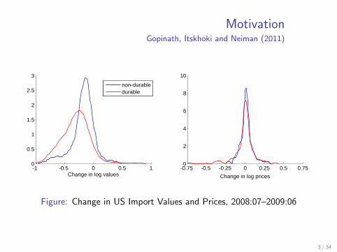
MotivationGopinath, Itskhoki and Neiman (2011)
-1 -0.5 0 0.5 10
0.5
1
1.5
2
2.5
3
Change in log values
IMP
OR
TS
-0.75 -0.5 -0.25 0 0.25 0.5 0.750
2
4
6
8
10
Change in log prices
-1 -0.5 0 0.5 10
0.5
1
1.5
2
2.5
3
Change in log values
EX
PO
RTS
-0.75 -0.5 -0.25 0 0.25 0.5 0.750
2
4
6
8
10
Change in log prices
non-durabledurable
Figure: Change in US Import Values and Prices, 2008:07–2009:06
3 / 34

Main Findings
• Assumptions
— Some degree of monopolistic power
— Lack of commitment by firms
— Discrete time periods between price setting
• Results
1 Endogenous markup dynamics
— markups decrease with the stock of durables
2 ‘Countercyclical’ markups in response to cost shocks
— incomplete pass-through
3 ‘Procyclical’ markups in response to demand shocks
4 Adjustment-cost-like effect on quantities
4 / 34

LiteratureDurable Monopoly Pricing
• Coase conjecture
— Coase (1972), Stokey (1981), Bulow (1982), Gul et al. (1986),Bond and Samuelson (1984)
— We focus on: ∆t � 0, δ > 0, dynamics
• Durable-good oligopoly pricing
— Gul (1987), Esteban (2003), Esteban and Shum (2007)
— We focus on: dynamics of markups, GE
• Macro models
— Caplin and Leahy (2006), Parker (2001)
— We focus on: general demand and market structures, GE
5 / 34
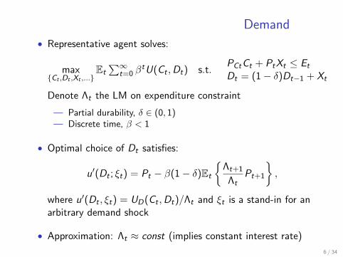
Demand
• Representative agent solves:
max{Ct ,Dt ,Xt ,...}
Et∑∞
t=0 βtU(Ct ,Dt) s.t.
PCtCt + PtXt ≤ Et
Dt = (1− δ)Dt−1 + Xt
Denote Λt the LM on expenditure constraint
— Partial durability, δ ∈ (0, 1)— Discrete time, β < 1
• Optimal choice of Dt satisfies:
u′(Dt ; ξt) = Pt − β(1− δ)Et
{Λt+1
ΛtPt+1
},
where u′(Dt , ξt) = UD(Ct ,Dt)/Λt and ξt is a stand-in for anarbitrary demand shock
• Approximation: Λt ≈ const (implies constant interest rate)
6 / 34
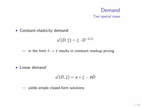
DemandTwo special cases
• Constant-elasticity demand:
u′(D, ξ) = ξ · D−1/σ
— in the limit δ → 1 results in constant markup pricing
• Linear demand:
u′(D, ξ) = a + ξ − bD
— yields simple closed-form solutions
7 / 34

Market Structure
• Market structure:
— Monopoly— Monopolistic competition— Homogenous-good Oligopoly
— Next time: differentiated-good oligopoly
• Equilibrium concept:
— Commitment (benchmark)— Discretion (Markov Perfect Equilibrium)
— Not for now: reputational equilibria under oligopoly
8 / 34

Durable Good MonopolyCommitment
• Optimal pricing with commitment
V C (D−1) = max{Pt ,Xt ,Dt}t≥0
E0
∞∑t=0
βt(Pt −Wt)Xt
subject to durable stock dynamics
Dt = Xt + (1− δ)Dt−1
and durable-good demand
u′(Dt , ξt) = Pt − β(1− δ)EtPt+1
and initial condition D−1 = 0
9 / 34

Commitment(continued)
• First-order optimality:
P0 : D0 − (1− δ)D−1 = λ0,
Pt , t ≥ 1 : Dt − (1− δ)Dt−1 = λt − (1− δ)λt−1,
Dt , t ≥ 0 : (Pt −Wt)− β(1− δ)Et{Pt+1 −Wt+1}= −λtu′′(Dt , ξt),
where λt is LM on demand constraint
• Given initial condition (D−1 = 0), we have λt ≡ Dt
(commitment ∼ leasing)
• Optimality condition:
(Pt −Wt)− β(1− δ)Et{Pt+1 −Wt+1} = −Dtu′′(Dt , ξt)︸ ︷︷ ︸
≡ 1σt
u′(Dt ,ξt)
10 / 34

Commitment(continued)
• Combining optimality condition with demand:
u′(Dt , ξt) + Dtu′′(Dt , ξt) = Wt − β(1− δ)EtWt+1
Pt − β(1− δ)EtPt+1 = u′(Dt , ξt)
• Contrast with marginal cost pricing:
u′(Dt , ξt) = Wt − β(1− δ)EtWt+1
Proposition
Durable pricing with commitment featuresno endogenous dynamics:
— Pt ≡ P when there are no shocks (Wt and ξt constant)
— Dt−1 does not affect Pt , controlling for Wt and ξt
— Pt inherits the exogenous persistence of Wt and ξt details
11 / 34

CommitmentTwo special cases
• Constant-elasticity demand
−→ constant markup pricing
Pt =σ
σ − 1Wt
• Linear demand
Pt =1
2
[a
1− β(1− δ)+
ξt1− ρξβ(1− δ)
+ Wt
]— response to cost shocks does not depend on δ— level of markup increases with durability
12 / 34

Durable Good MonopolyDiscretion
• Time inconsistency problem:— demand depends on expected price tomorrow— firm wants to promise high price tomorrow— but tomorrow it fails to internalize the effect of price on
previous-period demand— firm competes with itself across time and in the limit of
continuous time firm loses all monopoly power (Coase)
• Solution concept:— consumers are infinitesimal, form rational expectations about
future prices and purchase durables according to demand— the firm set today’s price to maximize value anticipating its
inability to commit to future prices— accumulated stock of durables is the state variable— Markov Perfect Equilibrium
• Optimal price duration? Commitment versus flexibility13 / 34

Discretion(continued)
• Formally, the problem of the firm:
V (D−1,W , ξ) = max(P,X ,D)
{(P −W )X + βEV (D,W ′, ξ′)
}s.t. D = X + (1− δ)D−1,
u′(D, ξ) = P − β(1− δ)Etp(D,W ′, ξ′)
• Equilibrium requirement:
p(D−1,W , ξ) = arg max(P,X ,D)
{(P −W )X + βEV (D,W ′, ξ′)
}is the equilibrium strategy of the firm given state variable
14 / 34

Discretion(continued)
• Optimality condition:
(Pt −Wt)−β(1− δ)Et{Pt+1 −Wt+1}
=(Dt − (1− δ)Dt−1
) 1
−ϕ′(Pt ,Wt , ξt),
where demand slope is
ϕ′(Pt ,Wt , ξt) =1
u′′(Dt , ξt) + β(1− δ)Etp′(Dt ,Wt+1, ξt+1)
— Perturbation argument
— Lack of commitment (contrast with leasing)
— State variable dynamics:
Dt = ϕ(p(Dt−1,Wt , ξt),Wt , ξt
)= f (Dt−1,Wt , ξt)
15 / 34

DiscretionGeneral Results
Proposition
(a) Steady state:
P =σ
σ − δκW ,
where σ ≡ −u′(D)
Du′′(D), κ ≡ 1 + β(1−δ)p′(D)
u′′(D)> 1, u′(D) = [1− β(1− δ)]P.
(b) Endogenous dynamics:
Dt−1 is state variable for pricing at t and p′(·,W , ξ) < 0.
16 / 34
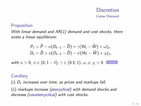
DiscretionLinear Demand
Proposition
With linear demand and AR(1) demand and cost shocks, thereexists a linear equilibrium:
Pt = P − α(Dt−1 − D) + γ(Wt − W ) + ωξt ,
Dt = D + φ(Dt−1 − D)− ψ(Wt − W ) + χξt ,
with α > 0, φ ∈ (0, 1− δ), γ ∈ (0.5, 1), ω, ψ, χ > 0. details
Corollary
(i) Dt increases over time, as prices and markups fall.
(ii) markups increase (procyclical) with demand shocks anddecrease (countercyclical) with cost shocks.
17 / 34

Monopolistic competition
• D-good is a CES aggregator of varieties:
Dt =
(∫ 1
0D
σ−1σ
it di
) σσ−1
• Two alternative assumptions:
(i) Durable aggregator: Dt = Xt + (1− δ)Dt−1.
Constant markup pricing (Barsky et al., 2007)
(ii) Durable varieties: Dit = Xit + (1− δ)Di,t−1.
Problem isomorphic to that of a monopolist with ξt related tothe equilibrium dynamics of Dt
18 / 34

Durable Good OligopolyCommitment (Cournot-Nash)
• Consider N symmetric firms producing a homogenous durablegood with constant marginal cost and no shocks
• Durable good dynamics
Dt = (1− δ)Dt−1 +∑N
i=1 xit
• A given firm commits to a sequence {xit} given the symmetricstrategy of the other N − 1 firms {xt}. In equilibrium, xt = xt
• In equilibrium, xt = 1N
(Dt − (1− δ)Dt−1
)and λt = Dt/N ⇒
(Pt −Wt)− β(1− δ)Et{Pt+1 −Wt+1} = −Dt
Nu′′(Dt , ξt)
19 / 34

Durable Good OligopolyDiscretion (Cournot-MPE)
• Under discretion, both competition within firm over time andbetween firms at a given t reduces markups
• A firm chooses x(D−) given the symmetric strategy x(D−) ofthe other N − 1 firms and equilibrium price next period p(D):
v(D−) = maxx ,D,P
{(P −W )x + βv(D)}
s.t. D = (1− δ)D− + (N − 1)x(D−) + x
P = u′(D) + β(1− δ)Ep(D)
• The solution to this problem in equilibrium yields:
x(D−) = x(D−), P = p(D−),
D = f (D−) = (1− δ)D− + Nx(D−)
20 / 34

Durable Good OligopolyDiscretion (Cournot-MPE)
• Optimality condition for a firm:
(P −W )−β[(1− δ) + (N − 1)x ′(D)
](P ′ −W ′)
= x(D−)(− u′′(D)− β(1− δ)p′(D)
)• Impose equilibrium:
x(D−) = x(D−) =1
N
(f (D−)− (1− δ)D
)• Then equilibrium dynamics is characterized by
u′(Dt) = Pt − β(1− δ)Pt+1,
(Pt −W )−β(Pt+1 −W )
(1− δ
N+
N − 1
Nf ′(Dt)
)=
Dt − (1− δ)Dt−1
N
1
−ϕ′(Pt),
where Dt = f (Dt−1), Pt = p(Dt−1) and ϕ(·) = f(p−1(·)
).
21 / 34
Durable Good OligopolyLinear Demand
Proposition
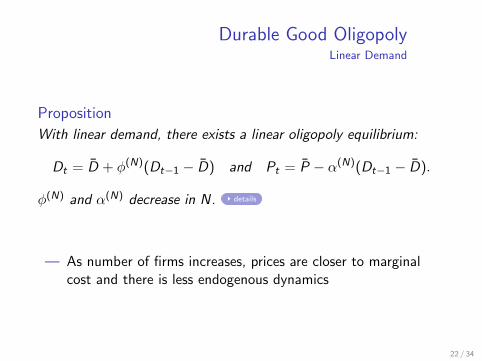
With linear demand, there exists a linear oligopoly equilibrium:
Dt = D + φ(N)(Dt−1 − D) and Pt = P − α(N)(Dt−1 − D).
φ(N) and α(N) decrease in N. details
— As number of firms increases, prices are closer to marginalcost and there is less endogenous dynamics
22 / 34

General Utility FunctionsApproximation
• Steady state markup cannot be solved for without p′(D).
• To compute the steady state markup exactly, we need toknow all derivatives of the policy function p(D) at D.
• Similar problem arises in hyperbolic discounting• Krusell, Kuruscu, and Smith (2002)• Judd (2004)• Polynomial approximations
• In the case of durables, polynomial approximations shouldwork perfectly.
• Each additional higher order term is suppressed by φn.
23 / 34

General Utility FunctionsApproximation
• In the case of monopoly, the transition function f (D) satisfies
(1− β (1− δ)) W − u′ (f (D))
f (D)− (1− δ) D− u′′ (f (D))
= β (1− δ)(1− β (1− δ)) W − u′ (f (f (D)))
f (f (D))− (1− δ) f (D)f ′ (f (D))
24 / 34

General Utility FunctionsApproximation
• Express f (D) as a power series.
• When Taylor expanded, the functional equation gives aninfinite number of conditions for the derivatives of f (D) at D
• The first one links D and f ′(D).
• The second one links D, f ′(D), and f ′′(D).
• The third one links D and the first three derivatives.
• Etc.
25 / 34

General Utility FunctionsApproximation
• If we set f (n)(D) to zero and solve the system, we make onlya small mistake proportional to φn, where φ ≡ f ′(D)
• In practice, only a couple of terms will be needed.
• When translated to the GE context, this means that it ispossible to solve GE models with durables and discretion, forarbitrary utility functions.
26 / 34

Numerical Example
• β = 0.9
• δ = 0.2
• Constant elasticity σ = 2
• Value function iteration on a grid, polynomial smoothing:
V (D−) = maxD
{(u′(D) + β(1− δ)p(D)−W
)(D − (1− δ)D−
)+ βV (D)
}Update V (D−) and D = f (D−), and calculate
p(D−) = u′(f (D−)
)+ β(1− δ)p
(f (D−)
)Polynomially smooth f (·) and p(·)
27 / 34
Numerical ExampleDynamics with no shocks
0 5 10 15 200
2
4
6
8
10
12
14
t
dt
dmct
dcommt
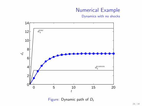
Figure: Dynamic path of Dt28 / 34

Numerical ExampleDynamics with no shocks
0 5 10 15 201
1.5
2
2.5
t
pt
p = w
p = σσ−1
w
Figure: Dynamic path of Pt
28 / 34

Numerical ExampleUnexpected permanent cost increase
−10 −5 0 5 10 15 200.9
1
1.1
1.2
1.3
1.4
1.5
Time, t
Wt,Pt
Wt
Pt
Figure: Response of Pt
29 / 34

Numerical ExampleUnexpected permanent cost increase
−10 −5 0 5 10 15 201.1
1.15
1.2
1.25
1.3
Time, t
Markup,Pt/W
t
Figure: Response of markup, Pt/Wt
29 / 34

Numerical ExampleUnexpected permanent cost increase
−10 −5 0 5 10 15 200
2
4
6
8
10
12
14
Time, t
Durable
stock,D
t
Dmct
Dt
Dcommt
Figure: Response of Dt
29 / 34
Numerical ExampleUnexpected permanent demand increase
−10 −5 0 5 10 15 201.2
1.225
1.25
1.275
1.3
Time, t
Price
andmarkup,PtandPt/W
t
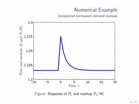
Figure: Response of Pt and markup Pt/Wt
30 / 34

Numerical ExampleUnexpected permanent demand increase
−10 −5 0 5 10 15 200
5
10
15
20
Time, t
Durable
stock,D
t
Dcommt
Dt
Dmct
Figure: Response of Dt
30 / 34

Numerical ExampleStochastic cost shocks
Table: Statistical properties
log(·) σ (%) ρ corr(·, log Wt)
Wage, Wt 4.9 0.80 1.00Price, Pt 5.1 0.90 0.88Markup, Pt/Wt 2.2 0.69 −0.19
Durable stock, Dt
— constant markup 15.5 0.79 −0.99— discretion 12.2 0.95 −0.75— ratio (disc/comm) 0.29
Durable purchases, Xt
— constant markup 70.7 -0.08 −0.31— discretion 21.4 0.57 −0.91— ratio (disc/comm) 0.16
31 / 34

Numerical ExampleStochastic cost shocks
Table: Pass-through
log Wt log Wt−1
log Pt 0.91log Pt 0.65 0.34
∆ log Wt ∆ log Wt−1
∆ log Pt 0.61∆ log Pt 0.63 0.15
32 / 34
Numerical ExampleStochastic demand shocks
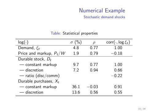
Table: Statistical properties
log(·) σ (%) ρ corr(·, log ξt)
Demand, ξt 4.8 0.77 1.00Price and markup, Pt/W 1.9 0.79 −0.18
Durable stock, Dt
— constant markup 9.7 0.77 1.00— discretion 7.2 0.94 0.66— ratio (disc/comm) −0.22
Durable purchases, Xt
— constant markup 36.1 −0.03 0.91— discretion 13.6 0.56 0.55
33 / 34

Conclusion
• Durable monopoly pricing results in endogenous dynamics
• Procyclical markups in response to demand shocks
• Countercyclical markups in response to cost shocks(incomplete pass-through)
• Oligopoly: endogenous dynamics dies out with N
• Next steps: general equilibrium, quantitative evaluation
34 / 34