Price Theory in Economics∗

Thomas A. Weber†

Forthcoming in: Ozer, O., Phillips, R. (eds.) The Oxford Handbook of Pricing Management, Oxford University Press.

And there is all the difference in the worldbetween paying and being paid.The act of paying is perhapsthe most uncomfortable infliction (...)But being paid, —what will compare with it?The urbane activity with which man receives moneyis really marvellous.

Herman Melville, Moby Dick

1 Origin of Value and Prices

Price theory is concerned with explaining economic activity in terms of the creation and transferof value, which includes the trade of goods and services between different economic agents. Apuzzling question addressed by price theory is, for example: why is water so cheap and diamondsare so expensive, even though water is critical for survival and diamonds are not? In a discussionof this well-known ‘Diamond-Water Paradox,’ Adam Smith (1776) observes that

[t]he word value, it is to be observed, has two different meanings, and sometimesexpresses the utility of some particular object, and sometimes the power of purchasingother goods which the possession of that object conveys. The one may be called “valuein use;” the other, “value in exchange.” (p. 31)

For him, diamonds and other precious stones derive their value from their relative scarcity andthe intensity of labor required to extract them. Labor therefore forms the basic unit of theexchange value of goods (or ‘items’), which determines therefore their ‘real prices.’ The ‘nominalprice’ of an item in Smith’s view is connected to the value of the currency used to trade it andmight therefore fluctuate. In this labor theory of value the Diamond-Water Paradox is resolvedby noting that it is much more difficult, in terms of labor, to acquire one kilogram of diamondsthan one kilogram of water.

∗The author would like to thank Naveed Chehrazi, Martin Grossman, and several anonymous referees forhelpful comments and suggestions.

†Chair of Operations, Economics and Strategy, Ecole Polytechnique Federale de Lausanne, Station 5, CDM-ODY 1.01B, CH-1015 Lausanne, Switzerland. E-mail: thomas.weber@epfl.ch.

1

About a century later, the work of Carl Menger, William Stanley Jevons, and Leon Walrasbrought a different resolution of the Diamond-Water Paradox, based on marginal utility ratherthan labor. Menger (1871) points out that the value of an item is intrinsically linked to its utility‘at the margin.’ While the first units of water are critical for the survival of an individual, theutility for additional units quickly decreases, which explains the difference in the value of waterand diamonds. Commenting on the high price of pearls, Jevons (1881) asks “[d]o men dive forpearls because pearls fetch a high price, or do pearls fetch a high price because men must dive inorder to get them?” (p. 102), and he concludes that “[t]he labour which is required to get moreof a commodity governs the supply of it; the supply determines whether people do or do notwant more of it eagerly; and this eagerness of want or demand governs value” (p. 103). Walras(1874/77) links the idea of price to the value of an object in an exchange economy by noting thatthe market price of a good tends to increase as long as there is a positive excess demand, whileit tends to decrease when there is a positive excess supply. The associated adjustment process isgenerally referred to as Walrasian tatonnement (“groping”). Due to the mathematical precisionof his early presentation of the subject, Walras is generally recognized as the father of generalequilibrium theory.1

To understand the notion of price it is useful to abstract from the concept of money.2 Ina barter where one person trades a quantity x1 of good 1 for the quantity x2 of good 2, theratio x1/x2 corresponds to his price paid for good 2. If apples correspond to good 1 and bananasto good 2, then the ratio of the number of apples paid to the number of bananas obtained inreturn corresponds to the (average) price of one banana, measured in apples. The currency inthis barter economy is denominated in apples, so that the latter is called the numeraire good,the price of which is normalized to one.

The rest of this survey, which aims at providing a compact summary of the (sometimes tech-nical) concepts in price theory, is organized as follows. In Section 2, we introduce the conceptsof “rational preference” and “utility function” which are standard building blocks of models thatattempt to explain choice behavior. We then turn to the frictionless interaction of agents in mar-kets. Section 3 introduces the notion of a Walrasian equilibrium, where supply equals demandand market prices are determined (up to a common multiplicative constant) by the self-interestedbehavior of market participants. This equilibrium has remarkable efficiency properties, whichare summarized by the first and the second fundamental welfare theorems. In markets withuncertainty, as long as any desired future payoff profile can be constructed using portfolios oftraded securities, the Arrow-Debreu equilibrium directly extends the notion of a Walrasian equi-librium and inherits all of its efficiency properties. Otherwise, when markets are “incomplete,”as long as agents have “rational expectations” in the sense that they correctly anticipate theformation of prices, the Radner equilibrium may guarantee at least constrained economic effi-ciency. In Section 4 we consider the possibility of disequilibrium and Walrasian tatonnement as aprice-adjustment process in an otherwise stationary economy. Section 5 deals with the problemof “externalities,” where agents’ actions are payoff-relevant to other agents. The presence ofexternalities in markets tends to destroy the efficiency properties of the Walrasian equilibriumand even threaten its very existence. While in Sections 3 and 4 all agents (including consumersand firms) are assumed to be “price takers,” we consider strategic interactions between agentsin Sections 6 and 7, in the presence of complete and incomplete information, respectively. The

1The modern understanding of classical general equilibrium theory is well summarized by Debreu’s (1959)concise axiomatic presentation and by Arrow and Hahn’s (1971) more complete treatise. Mas-Colell (1985)provides an overview from a differentiable viewpoint, and McKenzie (2002) a more recent account of the theory.Friedman (1962/2007), Stigler (1966), and Hirshleifer et al. (2005) present ‘price theory’ at the intermediate level.

2Keynes’ (1936) theory of liquidity gives some reasons for the (perhaps somewhat puzzling) availability ofmoney, which, after all, cannot be directly consumed, but provides a fungible means of compensation in exchange.

2

discussion proceeds from optimal monopoly pricing (which involves the problems of screening,signaling, and, more generally, mechanism design when information is incomplete) to price com-petition between several firms, either in a level relationship when there are several oligopolistsin a market, or as an entry problem, when one incumbent can deter (or encourage) the entranceof other firms into the market. Section 8 deals with dynamic pricing issues, and in Section 9we mention some of the persistent behavioral irregularities that are not well captured by classi-cal price theory. Finally, Section 10 concludes and provides a number of directions from whichfurther research contributions may be expected.

2 Price-Taking Behavior and Choice

Normative predictions about what agents do, i.e., about their “choice behavior,” requires sometype of model. In Section 2.1, we introduce preferences and the concept of a utility function torepresent those preferences. Section 2.2 then presents the classical model of consumer choice interms of a “utility maximization problem” in an economy where agents take the prices of theavailable goods as given. In Section 2.3, we examine how choice predictions depend on the givenprices or on an agent’s wealth, an analysis which is referred to as “comparative statics.” Inreality it is only rarely possible to make a choice which achieves a desired outcome for sure. Theeffects of uncertainty, discussed in Section 2.4, are therefore important for our understandingof how rational agents behave in an economy. Decision problems faced by two typical agents,named Joe and Melanie, will serve as examples.

2.1 Rational Preferences

An agent’s preferences can be expressed by a partial order over a choice set X.3 For example,consider Joe’s preferences over the choice set X = Apple,Banana,Orange when deciding whichfruit to pick as a snack. Assuming that he prefers an apple to a banana and a banana to anorange, his preferences on X thus far can be expressed in the form

Apple ≽ Banana,

Banana ≽ Orange,

where ≽ denotes “is (weakly) preferred to.” However, these preferences are not complete, sincethey do not specify Joe’s predilection between an apple and an orange. If Joe prefers an orangeto an apple, then the relation

Orange ≽ Apple

completes the specification of Joe’s preference relation ≽ which is then defined for all pairs ofelements of X. When Joe is ambivalent about the choice between an apple and a banana, so thathe both prefers an apple to a banana (as noted above) and a banana to an apple (i.e., Apple ≽Banana and Banana ≽ Apple both hold), we say that he is indifferent between the two fruitsand write Apple ∼ Banana. On the other hand, if Apple ≽ Banana holds but Banana ≽ Appleis not true, then Joe is clearly not indifferent: he strictly prefers an apple to a banana, which isdenoted by

Apple ≻ Banana.

If the last relation holds true, a problem arises because Joe’s preferences are now such that hestrictly prefers an apple to a banana, weakly prefers a banana to an orange, and at the same time

3Fishburn (1970) and Kreps (1988) provide more in-depth overviews of choice theory.

3

weakly prefers an orange to an apple. Thus, Joe would be happy to get an orange in exchangefor an apple. Then he would willingly take a banana for his orange, and, finally, pay a smallamount of money (or a tiny piece of an apple) to convert his banana back into an apple. Thiscycle, generated by the intransitivity of his preference relation, leads to difficulties when tryingto describe Joe’s behavior as rational.4

Definition 1 A rational preference ≽ on the choice set X is a binary relationship defined forany pair of elements of X, such that for all x, y, z ∈ X: (i) x ≽ y or y ≽ x (Completeness),(ii) x ∼ x (Reflexivity), and (iii) x ≽ y and y ≽ z together imply that x ≽ z (Transitivity).

To make predictions about Joe’s choice behavior over complex choice sets, dealing directly withthe rational preference relation ≽ is from an analytical point of view unattractive, as it involvesmany pairwise comparisons. Instead of trying to determine all ‘undominated’ elements of Joe’schoice set, i.e., all elements that are such that no other element is strictly preferred, it would bemuch simpler if the magnitude of Joe’s liking of each possible choice x ∈ X was encoded as anumerical value of a ‘utility function’ u(x), so that Joe’s most preferred choices also maximizehis utility.

Definition 2 A utility function u : X → R represents the rational preference relation ≽ (on X)if for all x, y ∈ X:

x ≽ y if and only if u(x) ≥ u(y).

It is easy to show that as long as the choice set is finite, there always exists a utility representationof a rational preference relation onX.5 In addition, if u represents≽ onX, then for any increasingfunction φ : R → R the utility function v : X → R with v(x) = φ(u(x)) for all x ∈ X alsorepresents ≽ on X.

2.2 Utility Maximization

If Joe has a rational preference relation on X that is represented by the utility function u, inorder to predict his choice behavior it is enough to consider solutions of his utility maximization

4When aggregating the preferences of a society of at least three rational agents (over at least three items),Arrow’s (1951) seminal ‘impossibility theorem’ states that, no matter what the aggregation procedure may be,these cycles can in general be avoided only by declaring one agent a dictator or impose rational societal preferencesfrom the outside. For example, if one chooses pairwise majority voting as aggregation procedure, cycles canarise easily, as can be seen in the following well-known voting paradox, which dates back to Condorcet (1785).Consider three agents with rational preferences relations (≽1, ≽2, and ≽3, respectively) over elements in thechoice set X = A,B,C such that A ≻1 B ≻1 C, B ≻2 C ≻2 A, and C ≻3 A ≻3 B. However, simple majorityvoting between the different pairs of elements of X yields a societal preference relation ≽ such that A ≻ B,B ≻ C, and C ≻ A implying the existence of a ‘Condorcet cycle,’ i.e., by Definition 1 the preference relation ≽is intransitive and thus not rational.

5If X is not finite, it may be possible that no utility representation exists. Consider for example lexicographicpreferences defined on the two-dimensional choice set X = [0, 1] × [0, 1] as follows. Let (x1, x2), (x1, x2) ∈ X.

Suppose that (x1, x2) ≽ (x1, x2)def⇐⇒ (x1 > x1) or (x1 = x1 and x2 ≥ x2). For example, when comparing

used Ford Mustang cars, the first attribute might index a car’s horsepower and the second its color (measured asproximity to red). An individual with lexicographic preferences would always prefer a car with more horsepower.However, if two cars have the same horsepower, the individual prefers the model with the color that is closer tored. The intuition why there is no utility function representing such a preference relation is that for each fixedvalue of x1, there has to be a finite difference between the utility for (x1, 0) and (x1, 1). But there are more thancountably many of such differences, which when evaluated with any proposed utility function can be used to showthat the utility function must in fact be unbounded on the square, which leads to a contradiction. For moredetails, see Kreps (1988). In practice, this does not lead to problems, since it is usually possible to discretize thespace of attributes, which results in finite (or at least countable) choice sets.

4

problem (UMP),x∗ ∈ argmax

x∈Xu(x). (1)

Let us now think of Joe as a consumer with a wealth w that can be spent on a bundle x =(x1, . . . , xL) containing nonnegative quantities xl, l ∈ 1, . . . , L, of the L available consumptiongoods in the economy. We assume henceforth that Joe (and any other agent we discuss) strictlyprefers more of each good,6 so that his utility function is increasing in x. To simplify further, weassume that Joe takes the price pl of any good l as given, i.e., he is a price taker. Given a pricevector p = (p1, . . . , pL) he therefore maximizes his utility u(x) subject to the constraint that thevalue of his total consumption, equal to the dot-product p ·x, does not exceed his total (positive)wealth w. In other words, all feasible consumption bundles lie in his budget set

B(p, w) =x ∈ RL

+ : p · x ≤ w.

Joe’s so-called Walrasian demand correspondence is

x(p, w) = arg maxx∈B(p,w)

u(x). (2)

Depending on the uniqueness of the solutions to Joe’s UMP, the Walrasian demand correspon-dence may be multivalued. Optimality conditions for this constrained optimization problem canbe obtained by introducing the Lagrangian

L(x, λ, µ; p, w) = u(x)− λ(p · x− w) + µx,

where λ ∈ R+ is the Lagrange multiplier associated with the inequality constraint p · x ≤ wand µ = (µ1, . . . , µL) ∈ RL

+ the Lagrange multiplier associated with the nonnegativity con-straint x ≥ 0. The necessary optimality conditions are

∂L(x, λ, µ; p, w)∂xl

=∂u(x)

∂xl

− λpl + µl = 0, l ∈ 1, . . . , L. (3)

Together with the complementary slackness conditions

λ(p · x− w) = 0 (4)

andµlxl = 0, l ∈ 1, . . . , L, (5)

they can be used to construct Joe’s Walrasian demand correspondence. For this, we first note thatsince Joe’s utility function is increasing in x, the budget constraint is binding, i.e., p·x = w, at theoptimum (Walras’ Law). In particular, if Joe consumes positive amounts of all commodities, i.e.,if x ≫ 0,7 the complementary slackness condition (5) implies that µl = 0 for all l ∈ 1, . . . , L,so that by (3) (with λ > 0) we obtain that

MRSlj(x) =

∂u(x)∂xl

∂u(x)∂xj

=plpj, l, j ∈ 1, . . . , L, (6)

6More precisely, it is sufficient to assume that Joe’s preferences are ‘locally nonsatiated,’ meaning that in theneighborhood of any bundle x there is another bundle x (located at an arbitrarily close distance) that Joe strictlyprefers. The consequence of this assumption is that Joe values any small increase of his wealth.

7We use the following conventions for inequalities involving vectors x = (x1, . . . , xL) and x = (x1, . . . , xL):(i) x ≤ x ⇔ xi ≤ xi ∀ i; (ii) x < x ⇔ x ≤ x and ∃ j s.t. xj < xj ; and (iii) x ≪ x ⇔ xi < xi ∀ i.

5

where MRSlj(x) is called the marginal rate of substitution between good l and good j (evaluatedat x). Condition (6) means that the marginal rate of substitution between any two goods hasto be equal to the ratio of the corresponding prices. It is interesting to note that Joe’s marginalrate of substitution at the optimum would therefore be the same as Melanie’s if she were tosolve the same problem, even though her preferences might be very different from Joe’s. In otherwords, any consumer chooses his or her Walrasian demand vector such that L − 1 independentconditions in Eq. (6) are satisfied (e.g., for i = 1, j ∈ 2, . . . , L). The missing condition for thedetermination of the Walrasian demand correspondence is given by the budget constraint,

p · x = w. (7)

As an example, consider the case where Joe has a utility function u(x) = xα11 xα2

2 for consuminga bundle x = (x1, x2),

8 where α1, α2 ∈ (0, 1) are constants. Then Eqs. (6) and (7) immediatelyimply Joe’s Walrasian demand,

x(p, w) =

(α1w

(α1 + α2)p1,

α2w

(α1 + α2)p2

).

Note that the Lagrange multiplier λ for the UMP (2) corresponds to the increase in Joe’s indirectutility,9

v(p, w) = maxx∈B(p,w)

u(x). (8)

Indeed, by the well-known envelope theorem (Milgrom and Segal, 2002) we have that

∂v(p, w)

∂w=

∂L(x, λ, µ; p, w)∂w

= λ. (9)

Lagrange multipliers are sometimes also referred to as “shadow prices” of constraints. In thiscase, λ corresponds to the value of an additional dollar of budget as measured in terms of Joe’sutility. Its unit is therefore “utile” per dollar.

Let us now briefly consider the possibility of a corner solution to Joe’s utility maximizationproblem, i.e., his Walrasian demand vanishes for (at least) one good l. In that case, µl > 0 andtherefore

MRSlj(x) =λpl − µl

λpj=

plpj

(1− µl

λ

)<

plpj,

provided that xj > 0, i.e., Joe consumes a positive amount of good j.10 Thus, Joe’s marginalutility ∂u(x)/∂xl for good l, which is not consumed, is lower relative to his marginal utility forgood j that he does consume, when compared to a consumer (e.g., Melanie) who uses positiveamounts of both good l and good j. The latter consumer’s marginal rate of substitution is equalto the ratio of prices (pl/pj), whereas Joe’s marginal rate of substitution is strictly less. Thismeans that a consumer may choose to forego consumption of a certain good if its price is too highcompared to the price of other goods, so that it becomes ‘too expensive’ to adjust the marginalrate of substitution according to the (interior) optimality condition (6).

8This functional form, first proposed by Cobb and Douglas (1928) for identifying ‘production functions’ (cf. Sec-tion 3.2) rather than utility functions, is often used for its analytical simplicity and the fact that its parameterscan easily be identified using data (e.g., by a linear regression).

9Joe’s value function v(p, w) is called “indirect utility” because he does usually not have a direct utility forthe parameters p and w representing price and wealth, respectively, as they cannot be consumed directly. Yetthey influence the problem and v can be thought of as representing a rational preference relation over differentvalues of (p, w).

10Clearly, because his utility is increasing and his wealth is positive, he will always demand a positive amountof at least one good.

6

2.3 Comparative Statics

Samuelson (1941) describes ‘comparative statics’ as the task of examining how a decision variablechanges as a function of changes in parameter values. Examining the shifts of model predictionswith respect to parameter changes is at the heart of price theory. We illustrate the main compar-ative statics techniques for the utility maximization problem. Consider, for example, the questionof how Joe’s Walrasian demand x(p, w) changes as his wealth w increases. His demand xl(p, w)for good l is called normal if it is nondecreasing in w. If that demand is positive, the first-ordercondition (3) can be differentiated with respect to the parameter w (using Eq. (9)) to obtain

∂x(p, w)

∂w=(D2u(x(p, w))

)−1p∂2v(p, w)

∂w2=(D2u(x(p, w))

)−1p∂λ(p, w)

∂w.

If u is strongly concave, then ∂λ(p, w)/∂w ≤ 0,11 i.e., the shadow value of wealth is decreasingas more and more wealth is added, since the individual’s marginal utility for the additionalconsumption decreases.

Remark 1 A good that is not normal, i.e., for which demand decreases as wealth rises, is calledinferior. Typical examples of such goods are frozen foods and bus transportation. In somewhatof a misnomer a normal good is referred to as a superior (or luxury) good if its consumptionincreases more than proportionally with wealth. Typical examples are designer apparel andexpensive foods such as caviar or smoked salmon. In some cases the consumption of superiorgoods can drop to zero as price decreases. Luxury goods are often consumed as so-called positionalgoods, the value of which strongly depends on how they compare with the goods owned by others(Hirsch, 1976; Frank, 1985).

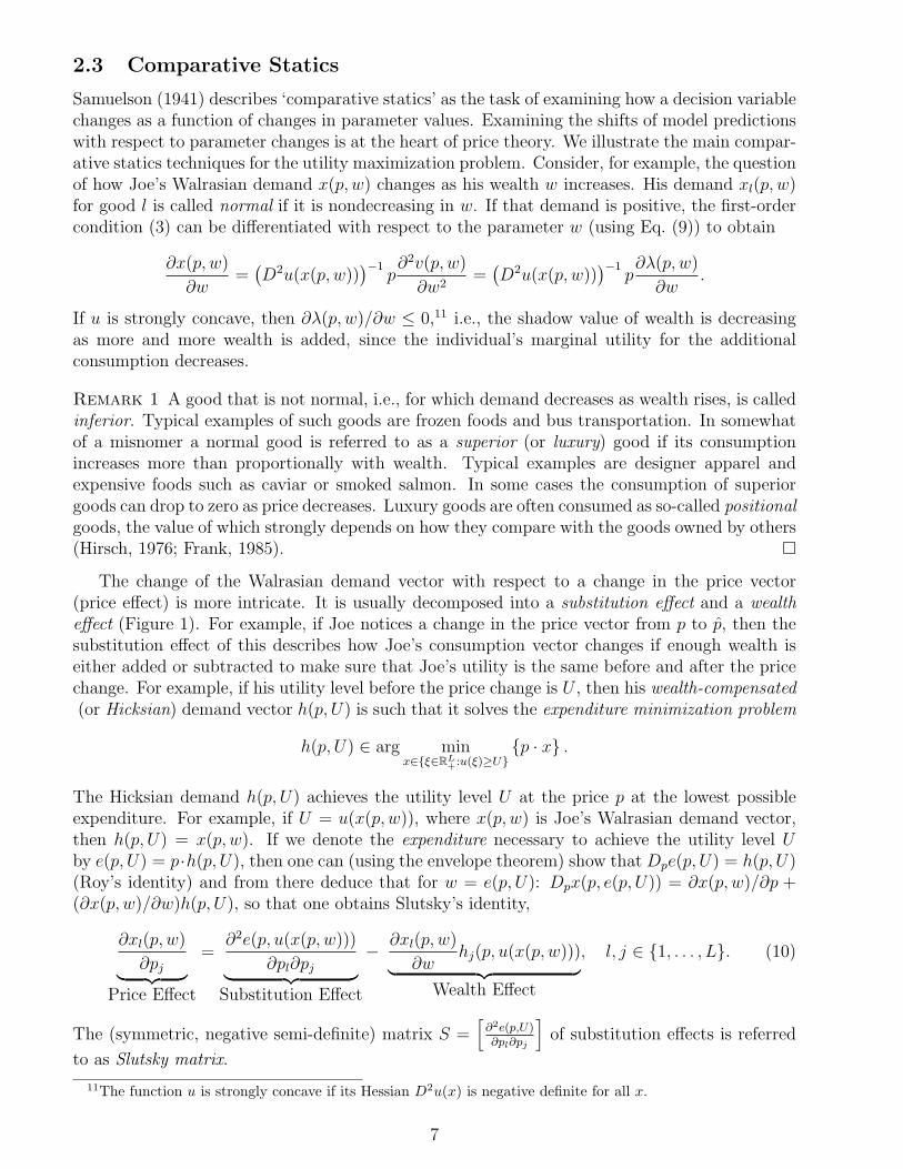
The change of the Walrasian demand vector with respect to a change in the price vector(price effect) is more intricate. It is usually decomposed into a substitution effect and a wealtheffect (Figure 1). For example, if Joe notices a change in the price vector from p to p, then thesubstitution effect of this describes how Joe’s consumption vector changes if enough wealth iseither added or subtracted to make sure that Joe’s utility is the same before and after the pricechange. For example, if his utility level before the price change is U , then his wealth-compensated(or Hicksian) demand vector h(p, U) is such that it solves the expenditure minimization problem

h(p, U) ∈ arg minx∈ξ∈RL

+:u(ξ)≥Up · x .

The Hicksian demand h(p, U) achieves the utility level U at the price p at the lowest possibleexpenditure. For example, if U = u(x(p, w)), where x(p, w) is Joe’s Walrasian demand vector,then h(p, U) = x(p, w). If we denote the expenditure necessary to achieve the utility level Uby e(p, U) = p·h(p, U), then one can (using the envelope theorem) show that Dpe(p, U) = h(p, U)(Roy’s identity) and from there deduce that for w = e(p, U): Dpx(p, e(p, U)) = ∂x(p, w)/∂p +(∂x(p, w)/∂w)h(p, U), so that one obtains Slutsky’s identity,

∂xl(p, w)

∂pj︸ ︷︷ ︸Price Effect

=∂2e(p, u(x(p, w)))

∂pl∂pj︸ ︷︷ ︸Substitution Effect

− ∂xl(p, w)

∂whj(p, u(x(p, w)))︸ ︷︷ ︸

Wealth Effect

, l, j ∈ 1, . . . , L. (10)

The (symmetric, negative semi-definite) matrix S =[∂2e(p,U)∂pl∂pj

]of substitution effects is referred

to as Slutsky matrix.

11The function u is strongly concave if its Hessian D2u(x) is negative definite for all x.

7

Iso-UtilityCurve

SubstitutionEffectWealth

Effect

Iso-UtilityCurve

Figure 1: Price effect as a result of a price increase for the first good, i.e., a shift from p = (p1, p2)to p = (p1, p2) (with p1 > p1 and p2 = p2), decomposed into substitution effect and wealth effectusing the compensated wealth w = e(p, u(x(p, w))).

Remark 2 A Giffen good is such that demand for it increases when its own price increases. Forexample, when the price of bread increases, a poor family might not be able to afford meat anylonger and therefore buy even more bread (Marshall, 1920). It is necessarily an inferior goodwith a negative wealth effect that overcompensates the substitution effect, resulting in a positiveprice effect.12 A related but somewhat different effect of increased consumption as a result of aprice increase is observed for a so-called Veblen good (e.g., a luxury car or expensive jewelry).Veblen (1899, p. 75) pointed out that “[c]onspicuous consumption of valuable goods is a meansof reputability to the gentleman of leisure.” Thus, similar to positional goods (cf. Remark 1),Veblen goods derive a portion of their utility from the price they cost (compared to other goods),since that implicitly limits their consumption by others.

We have seen that situations in which the dependence of decision variables is monotone inmodel parameters are especially noteworthy. The field of monotone comparative statics, whichinvestigates conditions on the primitives of a UMP (or similar problem) that guarantee suchmonotonicity, is therefore of special relevance for price theory (and economics as a whole).Monotone comparative statics was pioneered by Topkis (1968; 1998), who introduced the useof lattice-theoretic (so-called ‘ordinal’) methods, in particular the notion of supermodularity.13

Milgrom and Shannon (1994) provide sufficient and in some sense necessary conditions for themonotonicity of solutions to UMPs in terms of (quasi-)supermodularity of the objective func-

12Sørensen (2007) provides simple examples of utility functions which yield Giffen-good effects.13For any two vectors x, x ∈ RL

+, let x∧ x = minx, x be their componentwise minimum and x∨ x = maxx, xbe their componentwise maximum. The choice set X ⊂ R is a lattice if x, x ∈ X implies that x ∧ x ∈ Xand x ∨ x ∈ X. A function u : X → R is supermodular on a lattice X if u(x ∨ x) + u(x ∧ x) ≥ u(x) + u(x) forall x, x ∈ X.

8

tion, as long as the choice set is a lattice.14 Consider normal goods as an example for monotonecomparative statics. One can show that if u is strongly concave and supermodular, then the di-agonal elements of the Hessian of u are nonpositive and its off-diagonal elements are nonnegative(Samuelson, 1947). Strong concavity and supermodularity of u therefore imply that all goods arenormal goods (Chipman, 1977). Quah (2007) strengthens these results somewhat using ordinalmethods.

Remark 3 The practical interpretation of supermodularity is in terms of “complementarity.”To see this, consider a world with only two goods. Joe’s utility function u(x1, x2) has increasingdifferences if (x1, x2) ≫ (x1, x2) implies that u(x1, x2) − u(x1, x2) ≥ u(x1, x2) − u(x1, x2). Thatis, the presence of more of good 2 increases Joe’s utility response to variations in good 1. Forexample, loudspeakers and a receiver are complementary: without receiver an agent can be almostindifferent about the presence of loudspeakers, whereas when the receiver is present, it makes abig difference if loudspeakers are available or not. A parameterized function is supermodular if ithas increasing differences with respect to any variable-variable pair and any variable-parameterpair.

2.4 Effects of Uncertainty

So far, Joe’s choice problems have not involved any uncertainty. Yet, in many situations, insteadof a specific outcome a decision maker can select only an action, which results in a probabilitydistribution over many outcomes x ∈ X, or, equivalently, a random outcome x (or “lottery”)with realizations in X. Thus, given an action set A, the decision maker would like to selectan action a ∈ A so as to maximize the expected utility EU(a) = E[u(x)|a]. The conditionaldistributions F (x|a) defined for all (x, a) ∈ X × A are part of the primitives for this expected-utility maximization problem,

a∗ ∈ argmaxa∈A

EU(a) = argmaxa∈A

∫X

u(x)dF (x|a).

For example, if Joe’s action a ∈ A = [0, 1] represents the fraction of his wealth w that he caninvest in a risky asset that pays a random return r, distributed according to the distributionfunction G(r) = P (r ≤ r), then the distribution of his ex-post wealth x = w(1 + ar) conditionalon his action a is F (x|a) = G(( x

w− 1)/a) for a = 0 (and F (x|a = 0) = δ(x−w) and δ is a Dirac

distribution15), so that EU(a) =∫R u(x)dF (x|a) =

∫R u(w(1 + ar))dG(r) for all a ∈ A by simple

substitution. The solution to Joe’s classic portfolio investment problem depends on his attitudeto risk. Joe’s absolute risk aversion, defined by

ρ(x) = −u′′(x)/u′(x),

is a measure of how much he prefers a risk-free outcome to a risky lottery (in a neighborhoodof x). For example, in Joe’s portfolio investment problem, there exists an amount π(a) suchthat u(E[x|a] − π(a)) = EU(a), which is called the risk premium associated with Joe’s riskypayoff lottery as a consequence of his investment action a. If Joe’s absolute risk aversion is

14Monotone comparative statics under uncertainty is examined by Athey (2002); non-lattice domains are in-vestigated by Quah (2007). The latter is relevant, as even in a basic UMP of the form (2) for more than twocommodities the budget set B(p, w) is generally not a lattice. Strulovici and Weber (2008; 2010) provide meth-ods for finding a reparametrization of models that guarantees monotone comparative statics, even though modelsolutions in the initial parametrization may not be monotone.

15The (singular) Dirac distribution δ can be defined in terms of a limit, δ(x) = limε→0+ (ε− |x|)+ /ε2. Itcorresponds to a probability density with all its unit mass concentrated at the origin.

9

positive, so is his risk premium. The latter is the difference between the amount he is willing toaccept for sure and the actuarially fair value of his investment under action a.

Remark 4 In economic models, it is often convenient to assume that agents have constant abso-lute risk aversion (CARA) ρ > 0, which implies utility functions of the form u(x) = − exp(−ρx)for all monetary outcomes x ∈ R. The advantage is that the agents’ risk attitude is then inde-pendent of their starting wealth, which insulates models from “wealth effects.” Another commonassumption, when restricting attention to positive wealth levels (where x > 0), is that agentshave a relative risk aversion ρ(x) = xρ(x) that is constant. Such agents with constant relativerisk aversion (CRRA) ρ > 0 have utility functions of the form

u(x) =

lnx, if ρ = 1,x1−ρ/(1− ρ), otherwise.

For more details on decision making under risk, see Pratt (1964) and Gollier (2001). An axiomaticbase for expected utility maximization is provided in the pioneering work by Von Neumann andMorgenstern (1944).

3 Price Discovery in Markets

So far we have assumed that agents take the prices of all goods as given. Naturally, if goods arebought and sold in a market, prices will depend on the balance between demand and supply.Section 3.1 explains how prices are formed in a pure-exchange economy, in the absence of anyuncertainty. Under weak conditions, trade achieves an economically “efficient” outcome in thesense that it maximizes “welfare,” i.e., the sum of all agents’ utilities. Under some additionalassumptions, any efficient outcome can be achieved by trade, provided that a social planner canredistribute the agents’ endowments before trading starts. In Section 3.2, we note that theseinsights carry over to economies where firms producing all available goods are owned and operatedby the agents. Section 3.3 shows that these insights also apply in the presence of uncertainty,as long as the market is “complete” in the sense that all contingencies can be priced by bundlesof available goods. Section 3.4 provides some details about “incomplete” markets, where this isnot possible.

3.1 Pure Exchange

Consider an economy in which N agents can exchange goods in a market at no transactioncost. Each agent i has utility function ui(xi), where xi ∈ RL

+ is his consumption bundle, andis endowed with the bundle ωi ∈ RL

+ (his endowment). At the nonnegative price vector p thisagent’s Walrasian demand xi(p, p · ωi) is obtained by solving a UMP, where p · ωi is used as hiswealth. The market-clearing condition that supply must equal demand yields

N∑i=1

xi(p, p · ωi) =N∑i=1

ωi, (11)

and thus L relations (one for each good) that imply the price vector p = (p1, . . . , pL) up to acommon multiplicative constant, for only L− 1 components in Eq. (11) can be independent.

10

Definition 3 A Walrasian equilibrium (p, x) in a pure-exchange economy consists of an equi-librium price p ∈ RL

+ and an equilibrium allocation x = (x1, . . . , xN) such that

xi ∈ arg maxxi∈B(p,p·ωi)

ui(xi), i ∈ 1, . . . , N, (12)

andN∑i=1

(xi − ωi

)= 0. (13)

As an example, let us consider Joe (= agent 1) and Melanie (= agent 2) with identicalCobb-Douglas utility functions u1(x1, x2) = u2(x1, x2) = xα

1x1−α2 , where α ∈ (0, 1) is a given

constant. Suppose that Joe is endowed with the bundle ω1 = (1, 2) and Melanie with thebundle ω2 = (2, 1). The UMP (12) implies that agent i’s Walrasian demand vector (or “offercurve” (OC) when viewed as a function of price) is

xi(p, p · ωi) =

(αp · ωi

p1,(1− α)p · ωi

p2

).

From Eq. (13) we obtain that α(p1 + 2p2)/p1 + α(2p1 + p2)/p1 = 3, so that the ratio of pricesbecomes p1/p2 = α/(1 − α). By setting p1 = 1 (which amounts to considering good 1 as thenumeraire, cf. Section 1) we can therefore immediately determine a unique Walrasian equilib-rium (p, x), where p = (1, (1−α)/α) and xi = xi(p, p ·ωi) for i ∈ 1, 2, so that x1 = (2−α, 2−α)and x2 = (1+α, 1+α). The distribution of resources in a two-agent exchange economy, such as inthis example, can be conveniently displayed using the so-called Edgeworth-Bowley box diagramas shown in Figure 2.16 The figure also shows that the intersection of the agents’ offer curves lieson a “contract curve” which contains all “efficient” allocations as explained below.

The beauty of an exchange economy in which price takers interact freely without any trans-action cost is that a Walrasian equilibrium allocation cannot be improved upon in the followingsense. A feasible allocation x = (x1, . . . , xN) is said to be Pareto-efficient (relative to the set Xof feasible allocations) if there exists no other allocation x = (x1, . . . , xN) in X at which allindividuals are at least as well off as at x and at least one individual is better off. More precisely,x is Pareto-efficient if for all x ∈ X:17(

ui(xi) ≤ ui(xi) ∀ i)

⇒(ui(xi) = ui(xi) ∀ i

).

Adam Smith (1776, Book IV, Chapter 2) pointed to an “invisible hand” that leads individualsthrough their self-interest to implement socially optimal outcomes. A key result of price the-ory is that Walrasian equilibria, even though merely defined as a solution to individual utilitymaximization problems and a feasibility constraint (supply = demand), produce Pareto-efficientoutcomes.

Theorem 1 (First Fundamental Welfare Theorem) Any Walrasian equilibrium alloca-tion is Pareto-efficient.18

16A simple diagram of this sort was used by Edgeworth (1881, p. 28) to illustrate exchange allocations, and itwas later popularized by Bowley (1924).

17For each Pareto-efficient allocation x∗ ∈ X there exists a vector λ = (λ1, . . . , λN ) ≥ 0 of nonnegative weights

such that x∗ ∈ argmaxx∈X

∑Ni=1 λ

iui(xi). The last problem can be used to generate all such Pareto-efficient

allocations by varying λ.18The Pareto-efficiency of a Walrasian equilibrium allocation depends on the fact that consumer preferences

are locally nonsatiated (cf. Footnote 6).

11

Agent 1

Agent 2

2

2x

2

1x

1

1x

1

2x

OC1

OC2

x

Contract Curve

Iso-UtilityCurve

Figure 2: Offer curves (OC1 and OC2), Walrasian equilibrium, and Pareto-efficient allocations.

The intuition for the Pareto-efficiency of a Walrasian equilibrium allocation is best seen bycontradiction. Suppose that there exists an allocation x = (x1, x2) that would improve Joe’swell-being and leave Melanie at the utility level she enjoys under the Walrasian equilibriumallocation x = (x1, x2). By Walras’ Law, for Joe allocation x1 is not affordable under theequilibrium price p, so that p · x1 > p · x1. Furthermore, because Melanie is maximizing herutility in equilibrium, the alternative allocation x2 cannot leave her with any excess wealth, sothat p · x2 ≥ p · x2. Thus, the total value of the alternative allocation, p · (x1 + x2), is strictlygreater than the total value of the Walrasian equilibrium allocation, p · (x1 + x2). But thiscontradicts the fact that the total amount of goods in the economy does not depend on thechosen allocation, so that the total value in the economy is constant for a given price. Hence,we have obtained a contradiction, which implies that the Walrasian equilibrium allocation mustindeed be Pareto-efficient.

Theorem 2 (Second Fundamental Welfare Theorem) In a convex economy it is possi-ble to realize any given Pareto-efficient allocation as a Walrasian equilibrium allocation, after alump-sum wealth redistribution.

This important result rests on the assumption that the economy is convex, in the sense that eachconsumer’s sets of preferred goods (“upper contour sets”) relative to any feasible endowmentpoint is convex. The latter is necessary to guarantee the existence of an equilibrium price; it issatisfied if all consumers’ utility functions are concave.19 Figure 3 provides an example of howin a nonconvex economy it may not be possible to obtain a Walrasian equilibrium: as a functionof price, agent 1 switches discretely in his preference of good 1 and good 2, so that the market

19The proof of the second fundamental welfare theorem relies on the separating hyperplane theorem (statingthat there is always a plane that separates two convex sets which have no common interior points). In an economywith production (cf. Section 3.2) the firms’ production sets need to also be convex.

12

Agent 1

Agent 2

w

2

2x

2

1x

1

1x

1

2x

OC1

OC2

Iso-Utility

Curve

Figure 3: Nonconvex exchange economy without a Walrasian equilibrium.

cannot clear at any price (except when all its components are infinity, so that agents simply keeptheir endowments).

The set of Pareto-efficient allocations in an economy is often referred to as the “contract curve”(or Pareto set; cf. Footnote 17 and Figure 2). The subset of Pareto-efficient allocations whichpresent Pareto-improvements over the endowment allocation is called the core of the economy.While the first fundamental welfare theorem says that the Walrasian market outcome is in thecore of an economy, the second fundamental welfare theorem states that it is possible to rely onmarkets to implement any outcome in the Pareto set, provided that a lump-sum reallocation ofresources takes place before markets are opened.

3.2 Competitive Markets

The setting of the exchange economy in Section 3.1 does not feature any productive activity byfirms. Consider M such firms. Each firm m has a (nonempty) production set Y m ⊂ RL whichdescribes its production choices. For a feasible production choice ym = (ym1 , . . . , y

mL ), we say that

firm m produces good l if yml is nonnegative; otherwise it uses that good as an input. Thus, sinceit is generally not possible to produce goods without using any inputs, it is natural to requirethat Y ∩RL

+ ⊆ 0. This so-called no-free-lunch property of the production set Y m means that ifa firm produces goods without any inputs, then it cannot produce a positive amount of anything.Given a price vector p, firm m’s profit is p ·y. The firms’ profit-maximization problem is thereforeto find

ym(p) ∈ arg maxym∈Y m

p · y , m ∈ 1, . . . ,M. (14)

13

In a private-ownership economy each firm m is privately held. That is, each agent i owns thenonnegative share ϑi

m of firm m, such that

N∑i=1

ϑim = 1, m ∈ 1, . . . ,M. (15)

Definition 4 A Walrasian equilibrium (p, x, y) in a private-ownership economy is such that allagents maximize utility,

xi ∈ arg maxxi∈B(p,p·ωi+

∑Mm=1 ϑ

im(p·ym))

ui(xi), i ∈ 1, . . . , N,

all firms maximize profits,

ym ∈ arg maxym∈Y m

p · y , m ∈ 1, . . . ,M,

and the resulting allocation is feasible,

N∑i=1

(xi − ωi

)=

M∑m=1

ym.

The two fundamental welfare theorems continue to hold in the more general setting with produc-tion. The existence of a Walrasian equilibrium is guaranteed as long as there are no externalities(cf. Section 5) and the economy is convex (cf. Footnote 19).

3.3 Complete Markets

The agents’ consumption choice and the firms’ production decisions are generally subject touncertainty. As in Section 2.4, this may simply mean that agents maximize expected utility andfirms expected profits. However, in many situations the agents can use a market mechanismto trade before a random state of the world realizes. Arrow (1953) and Debreu (1953) haveshown that all the efficiency properties of the Walrasian equilibrium carry over to case withuncertainty, provided that ‘enough’ assets are available, a notion that will be made precise inthe definition of complete markets below (cf. Definition 5). For simplicity we assume that theuncertain state of the world, denoted by the random variable s, can have realizations in the finitestate space S = s1, . . . , sK. Agent i believes that state sk occurs with probability µi

k.We now develop a simple two-period model to understand how agents (or “traders”) can

trade in the face of uncertainty. Consider Joe (= agent 1), who initially owns firm 1, andMelanie (= agent 2), who initially owns firm 2. The state space S = s1, s2 contains onlytwo elements (i.e., K = 2). Let V m be the market value of firm m in period 1. The monetaryvalue of firm m in state sk is ωm

k . After trading of firm shares takes place in the first period,Joe and Melanie each hold a portfolio ϑi = (ϑi

1, ϑi2) of ownership shares in the firms. In the

second period all uncertainty realizes and each agent i can make consumption decisions usingthe wealth wi

k(ϑi) = ϑi

1ω1k + ϑi

2ω2k in state sk, obtaining the indirect utility vik(w

ik). Hence, in

period one, the traders Joe and Melanie, can trade firm shares as follows. Each trader i solvesthe expected utility maximization problem

ϑi(V ) ∈ arg maxϑi∈B((V 1,V 2),V i)

K∑k=1

µikv

ik(w

ik(ϑ

i))

.

14

Trader 1

Trader 2

w

Pareto-efficient allocations

Arrow-Debreu Equilibrium

45o

45o

Figure 4: Market for contingent claims.

If in addition the market-clearing condition (15) holds, then the resulting equilibrium (V , ϑ),with V = (V 1, V 2) and ϑ = (ϑ1(V ), ϑ2(V )), is called a rational expectations equilibrium.20 Inthis equilibrium, Joe and Melanie correctly anticipate the equilibrium market prices of the firmwhen making their market-share offers, just as in the Walrasian pure-exchange economy discussedin Section 3.1.

In the last example, Joe and Melanie each owned a so-called asset (or security), the definingcharacteristic of which is that it entitles the owner to a determined monetary payoff in eachstate of the world. All that matters for consumption after the conclusion of trade in the firstperiod is how much money an agent has available in each state. Thus, Joe and Melanie couldcome to the conclusion that instead of trading the firm shares, it would be more appropriate totrade directly in ‘state-contingent claims to wealth.’ If trader i holds a state-contingent claimportfolio ci = (ci1, . . . , c

iK), then in state sk that trader obtains the indirect utility vik(c

ik). In

the first period when trading in contingent claims takes place, the price for a claim to wealth instate sk is pk. Hence, each trader i has demand

ci ∈ arg maxci∈B(p,p·ωi)

K∑k=1

vik(cik)

, i ∈ 1, . . . , N, (16)

that maximizes expected utility. Eq. (16) and the market-clearing relation

N∑i=1

(ci − ωi

)= 0 (17)

together constitute the conditions for a Walrasian equilibrium (p, c) in the market of contingentclaims, referred to as Arrow-Debreu equilibrium (Figure 4). Using the insights from Section 2.2,note that the marginal rate of substitution between claims in state sk and claims in state sl

20The concept of rational expectations in economics originated with Muth (1961), and the rational expectationsequilibrium which is used here with Radner (1972).

15

equals the ratio of the corresponding market prices at an (interior) equilibrium,

MRSkl(ci) =

µikv

ik(c

ik)

µilv

il(c

il)

=pkpl.

This is independent of the agent i, so that after normalizing the market prices to sum to one,the prices p1, . . . , pK define a probability distribution over the states of the world, which isreferred to as equivalent martingale measure. While traders may disagree about their probabilityassessments for the different states of the world, they are in agreement about the equivalentmartingale measure in equilibrium.21

It is possible to go back and forth between the market for firm shares and the market forcontingent claims if and only if the system of equations ω1

1 · · · ωM1

......

ω1K · · · ωM

K

︸ ︷︷ ︸

Ω

ϑi1...

ϑiM

︸ ︷︷ ︸

ϑi

=

ci1...ciK

︸ ︷︷ ︸

ci

possesses a solution, or, equivalently, if the asset return matrix Ω is of rank K.

Definition 5 (i) If the K×M asset return matrix Ω has rank K, then the market for contingentclaims is called complete. (ii) A Walrasian equilibrium (p, c) in a complete market for contingentclaims, satisfying Eqs. (16) and (17), is called an Arrow-Debreu equilibrium.

The concept of completeness can easily be extended to multi-period economies (Debreu, 1959),where time is indexed by t ∈ 0, 1, . . . , T. The state of the world st at time t ≥ 1 can dependon the state of the world st−1 at time t− 1. As the states of the world successively realize, theyplow a path through an event tree. In a complete market it is possible to trade claims that arecontingent on any possible path in the event tree.

3.4 Incomplete Markets

If the market is not complete (in the sense of Definition 5(i)), the rational expectations equilib-rium (also referred to as Radner equilibrium) may produce a Pareto-inefficient allocation. Thereason is that if there are more states of the world than linearly independent assets, then it isgenerally not possible for agents to trade contracts that diversify the risks in the economy to thedesirable degree. To see this, consider two risk-averse agents in an economy with two or morestates, where there are no firms (or assets) that can be traded, so that there is no possibilityfor mutual insurance. The latter would be the Pareto-efficient outcome in an Arrow-Debreuequilibrium when contingent claims are available.

The consequence of market incompleteness is that agents in the economy cannot perfectlytrade contingent claims. One can show that, in an economy with only two periods, a rationalexpectations equilibrium is “constrained Pareto-efficient,” in the sense that trade in the firstperiod is such that agents obtain a Pareto-efficient allocation in expected utilities, subject to theavailable assets.22

21Aumann (1976) points out that, in a statistical framework, it is in fact impossible for agents to “agree todisagree” on probability distributions if all the evidence is made available to all agents. Naturally, without suchinformation exchange, the agents’ subjective probabilities may vary significantly.

22In multi-period (and/or multi-good) economies, rational expectations equilibria are not even guaranteed tobe constrained Pareto-efficient (for details see, e.g., Magill and Quinzii (1996)).

16

The question naturally arises as to how assets should be priced when markets are incomplete.The answer is that depending on the agents’ beliefs in the market, a number of different prices arepossible. In general, it is reasonable to assume that, as long as transaction costs are negligible,asset prices do not allow for arbitrage possibilities, i.e., ways of obtaining a risk-free profit throughmere trading of assets. For concreteness, let us assume that there are three assets and that eachasset m ∈ 1, 2, 3 is characterized by a return vector ωm = (ωm

1 , . . . , ωmK) which specifies the

payoffs for all possible states s1, . . . , sK . In addition, suppose that the return vector of the thirdasset is a linear combination of the return vectors of the first two assets, so that

ω3 = ϕ1ω1 + ϕ2ω2

for some constants ϕ1 and ϕ2. If V m is the market price of asset m, then clearly we must havethat

V 3 = ϕ1V 1 + ϕ2V 2

in order to exclude arbitrage opportunities. In other words, if the state-contingent payoffs ofan asset can be replicated by a portfolio of other assets in the economy, then the price of theasset must equal the price of the portfolio.23 Accordingly, no-arbitrage pricing refers to theselection of prices that do not allow for risk-free returns resulting from merely buying and sellingavailable assets.24 But no-arbitrage pricing in an incomplete market alone provides only anupper and a lower bound for the price of an asset. Additional model structure (e.g., provided bygeneral equilibrium assumptions or through the selection of an admissible equivalent martingalemeasure) is required to pinpoint a particular asset price. Arbitrage pricing theory (Ross, 1976;Roll and Ross, 1980) postulates that the expected value of assets can be well estimated by alinear combination of fundamental macro-economic factors (e.g., price indices). The sensitivityof each factor is governed by its so-called β-coefficient.

A rational expectations equilibrium in an economy in which the ‘fundamentals of the econ-omy,’ i.e., the agents’ utilities and endowments, do not depend on several states, but consump-tions are different across those states, is called a sunspot equilibrium (Cass and Shell, 1983).The idea is that observable signals that bear no direct effect on the economy may be able toinfluence prices through traders’ expectations. In light of well-known boom-bust phenomena instock markets, it is needless to point out that traders’ expectations are critical in practice for theformation of prices. When market prices are at odds with the intrinsic value of an asset (i.e., thevalue implied by its payoff vector), it is likely that traders are trading in a “speculative bubble”because of self-fulfilling expectations about the further price development. Well-known examplesof speculative bubbles include the tulip mania in the Netherlands in 1637 (Garber, 1990), thedot-com bubble at the turn of last century (Shiller, 2005; Malkiel, 2007), and, more recently,the U.S. housing bubble (Sowell, 2010). John Maynard Keynes (1936) offered the followingcomparison:

“... professional investment may be likened to those newspaper competitions in whichthe competitors have to pick out the six prettiest faces from a hundred photographs,the prize being awarded to the competitor whose choice most nearly corresponds to

23To see this, assume for example that the market price V 3 is greater than ϕ1V 1 + ϕ2V 2. Thus, if a traderholds a portfolio with quantities q1 = ϕ1V 3 of asset 1, q2 = ϕ2V 3 of asset 2, and q3 = −(ϕ1V 1+ϕ2V 2) of asset 3,

then the value of that portfolio vanishes, as∑3

m=1 qmV m = 0. However, provided an equivalent martingale

measure p1, . . . , pM (cf. Section 3.3) the total return of the portfolio,∑K

k=1 pkVmωm

k qk = pkω3k(V

3 − (ϕ1V 1 +ϕ2V 2)), is positive for each state sk.

24Another approach to asset pricing is Luenberger’s (2001; 2002) zero-level pricing method, based on thewidely used Capital Asset Pricing Model (Markowitz, 1952; Tobin, 1958; Sharpe 1964). It relies on the geometricprojection of the prices of ‘similar’ traded assets.

17

the average preferences of the competitors as a whole; so that each competitor hasto pick, not those faces which he himself finds prettiest, but those which he thinkslikeliest to catch the fancy of the other competitors, all of whom are looking at theproblem from the same point of view. It is not a case of choosing those which, to thebest of one’s judgment, are really the prettiest, nor even those which average opiniongenuinely thinks the prettiest. We have reached the third degree where we devoteour intelligences to anticipating what average opinion expects the average opinion tobe. And there are some, I believe, who practise the fourth, fifth and higher degrees”(p. 156).

In this “beauty contest,” superior returns are awarded to the trader who correctly anticipatesmarket sentiment. For additional details on asset pricing see, e.g., Duffie (1988; 2001).

4 Disequilibrium and Price Adjustments

In practice, we cannot expect markets always to be in equilibrium, especially when agents arefree to enter and exit, economic conditions may change over time, and not all market participantspossess the same information. Section 4.1 specifies a possible price adjustment process, referredto as “tatonnement,” that tends to attain a Walrasian equilibrium asymptotically over time. InSection 4.2, we summarize important insights about the strategic use of private information inmarkets, e.g., the fundamental result that trade might not be possible at all if all agents arerational and some hold extra information.

4.1 Walrasian Tatonnement

In real life there is no reason to believe that markets always clear. At a given price it may be thatthere is either excess demand or excess supply, which in turn should lead to an adjustment ofprices and/or quantities. While it is relatively simple to agree about the notion of a static Wal-rasian equilibrium, which is based on self-interested behavior of price-taking agents and firms aswell as a market-clearing condition, there are multiple ways of modelling the adjustment dynam-ics when markets do not clear. Walras (1874/77) was the first to formalize a price-adjustmentprocess by postulating that the change in the price of good l ∈ 1, . . . , L is proportional to theexcess demand zl of good l, where (suppressing all dependencies from entities other than price)

zl(p) =N∑i=1

(xil(p)− ωi

l

)−

m∑m=1

yml (p).

This leads to an adjustment process, which in continuous time can be described by a system of Ldifferential equations,

pl = κlzl(p), l ∈ 1, . . . , L. (18)

This process is commonly referred to as a Walrasian tatonnement. The positive constants κl

determine the speed of the adjustment process for each good l.25 One can show that if theWalrasian equilibrium price vector p is unique, and if p · z(p) > 0 for any p not proportional to p,

25It may be useful to normalize the price vector p(t) such that p21(t)+ · · ·+ p2L(t) ≡ 1, since then d(p21(t)+ · · ·+p2L(t))/dt = 2 p(t) · z(p(t)) ≡ 0 (with z = (z1, . . . , zL)). Under this normalization any trajectory p(t) remains inthe ‘invariant’ set S = p : (p1)

2 + · · ·+ (pL)2 = 1.

18

then a solution trajectory p(t) of the Walrasian tatonnement (18) converges to p, in the sensethat

limt→∞

p(t) = p.

As an illustration, we continue the example of a two-agent two-good exchange economy withCobb-Douglas utility functions in Section 3.1. The tatonnement dynamics in Eq. (18) become

p1 = 3κ1 (α(p1 + p2)/p1 − 1) ,p2 = 3κ2 ((1− α)(p1 + p2)/p2 − 1) ,

where κ1, κ2 > 0 are appropriate constants. It is easy to see that p1/p2 < α/(1 − α) impliesthat p1 > 0 (and that p2 < 0) and vice versa. In (p1, p2)-space we therefore obtain that atrajectory p2(p1) (starting at any given price vector) is described by

dp2(p1)

dp1=

3κ2 ((1− α)(p1 + p2)/p2 − 1)

3κ1 (α(p1 + p2)/p1 − 1)= −κ2

κ1

p1p2.

It follows a concentric circular segment, eventually approaching a ‘separatrix’ defined by p1/p2 =α/(1− α) (cf. Figure 5). We see that when the price of good 1 is too low relative to the price ofgood 2, then due to the positive excess demand, p1 will adjust upwards until the excess demandfor that good vanishes, which – by the market-clearing condition – implies that the excess demandfor the other good also vanishes, so that we have arrived at an equilibrium.26

Walrasian price-adjustment processes have been tested empirically. Joyce (1984) reportsexperimental results in an environment with consumers and producers that show that for asingle unit of a good the tatonnement can produce close to Pareto-efficient prices, and that theprocess has strong convergence properties. Bronfman et al. (1996) consider the multi-unit caseand find that the efficiency properties of the adjustment process depend substantially on how thisprocess is defined. Eaves and Williams (2007) analyze Walrasian tatonnement auctions at theTokyo Grain Exchange run in 1997/98 and find that price formation is similar to the normativepredictions in continuous double auctions.

We note that it is also possible to consider quantity adjustments instead of price adjustments(Marshall, 1920). The resulting quantity-adjustment dynamics are sometimes referred to asMarshallian dynamics (in contrast to the Walrasian dynamics for price adjustments).

4.2 Information Transmission in Markets

It is an economic reality that different market participants are likely to have different informationabout the assets that are up for trade. Thus, in a market for used cars, sellers may have moreinformation than buyers. For simplicity, let us consider such a market, where cars are either ofvalue 0 or of value 1, but it is impossible for buyers to tell which one is which until after thetransaction has taken place. Let φ ∈ (0, 1) be the fraction of sellers who sell “lemons” (i.e., carsof zero value) and let c ∈ (0, 1) be the opportunity cost of a seller who sells a high-value car.Then, if 1− φ < c, there is no price p at which buyers would want to buy and high-value sellers

26A Walrasian equilibrium price is locally asymptotically stable if, when starting in a neighborhood of thisprice, Walrasian tatonnement yields price trajectories that converge toward the equilibrium price. A suffi-cient condition for local asymptotic stability (i.e., convergence) is that the linearized system p = A (p− p)corresponding to the right-hand side of Eq. (18) around the Walrasian equilibrium price p is such that thelinear system matrix A has only eigenvalues with negative real parts. In the example, we have that A =

3α

[−ακ1/(1− α) κ1

κ2 −ακ2/(1− α)

], the eigenvalues of which have negative real parts for all κ1, κ2 > 0 and

all α ∈ (0, 1). For more details on the analysis of dynamic systems, see, e.g., Weber (2011).

19

Figure 5: Walrasian price adjustment process with asymptotic convergence of prices.

would want to sell. Indeed, high-value sellers sell only if p ≥ c. Lemons sellers simply imitatehigh-value sellers and also charge p for their cars (they would be willing to sell at any nonnegativeprice). As a consequence, the buyers stand to obtain the negative expected value (1−φ)−p frombuying a car in this market, which implies that they do not buy. Hence, the market for usedcars fails, in the sense that only lemons can be traded, if there are too many lemons comparedto high-value cars (Akerlof 1970). This self-inflicted disappearance of high-value items from themarket is called “adverse selection.”

In the context of Walrasian markets in the absence of nonrational (“noise”) traders, and aslong as the way in which traders acquire private information about traded assets is commonknowledge, Milgrom and Stokey (1982) show that none of the traders is in a position to profitfrom the private information, as any attempt to trade will lead to a correct anticipation ofmarket prices. This implies that private information cannot yield a positive return. Since thistheoretical no-trade theorem is in sharp contrast to the reality found in most financial markets,where superior information tends to yield positive (though sometimes illegal) returns, the missingingredient are irrational “noise traders,” willing to trade without concerns about the privateinformation available to other traders (e.g., for institutional reasons).

What information can be communicated in a market? Hayek (1945, p. 526) points out thatone should in fact consider the “price system” in a market as “a mechanism for communicatinginformation.” The price system is useful under uncertainty, since (as we have seen in Section 3)markets generally exist not only for the purpose of allocating resources, but also to provide traderswith the possibility of mutual insurance (Hurwicz 1960). To understand the informational roleof prices under uncertainty, let us consider a market as in Section 3.4, where N strategic traders(“investors”) and a number of nonstrategic traders (“noise traders”) trade financial securities thathave state-contingent payoffs. Each investor i may possess information about the future payoffof these securities in the form of a private signal zi, which, conditional on the true state of theworld, is independent of any other investor j’s private signal zj. In the classical model discussed

20

thus far, at any given market price vector p for the available securities, agent i has the Walrasiandemand xi(p, ωi; zi), which – in addition to his endowment ωi – also depends on the realization zi

of his private signal. However, an investor i who conditions his demand only on the realized priceand his private information would ignore the process by which the other agents arrive at theirdemands, which help establish the market price, which in equilibrium must depend on the fullinformation vector z = (z1, . . . , zN). For example, if investor i’s private information leads himto be very optimistic about the market outlook, then at any given price p his demand will behigh. Yet, if a very low market price p is observed, investor i obtains the valuable insight that allother investors’ signal realizations must have been rather dim, which means that his informationis likely to be an extreme value from a statistical point of view. Grossman and Stiglitz (1980)therefore conclude that in a rational-expectations equilibrium each investor i’s demand mustbe of the form xi(p, ωi; zi, p(z)), i.e., it will depend on the way in which the equilibrium priceincorporates the available information.27 While in an economy where private information is freelyavailable this may result in the price to fully reveal the entire information available in the market(because, for example, it depends only on an average of the investors’ information; Leland andPyle 1976), this does not hold when information is costly. Grossman and Stiglitz show thatin the presence of a (possibly even small) cost of acquiring private information, prices fail toaggregate all the information in the market, so that a rational expectations equilibrium cannotbe ‘informationally efficient.’28

The question naturally arises of how to use private information in an effective way, especiallyif one can do so over time.29 Kyle (1985) develops a seminal model of insider trading where oneinformed investor uses his inside information in a measured way over a finite time horizon soas to not be imitated by other rational investors. Another option an informed investor has forusing private information is to sell it to other investors. Admati and Pfleiderer (1986) show thatit may be best for the informed investor to degrade this information (by adding noise) beforeselling it, in order to protect his own trading interests.

Remark 5 Arrow (1963) realized that there are fundamental difficulties when trying to sellinformation from an informed party to an uninformed party, perhaps foreshadowing the no-tradetheorem discussed earlier. Indeed, if the seller of information just claims to have the information,then a buyer may have no reason to believe the seller.30 The seller therefore may have to ‘prove’that the information is really available, e.g., by acting on it in a market (taking large positions

27In an actual financial market (such as the New York Stock Exchange), investors can submit their offer curvesin terms of ‘limit orders,’ which specify the number of shares of each given asset that the investor is willing tobuy at a given price.

28In the absence of randomness a rational expectations equilibrium may even fail to exist. Indeed, if no investorexpends the cost to become informed, then the equilibrium price reveals nothing about the true value of the asset,which produces an incentive for investors to become informed (provided the cost is small enough). On the otherhand, if all other investors become informed, then, due to the nonstochastic nature of the underlying values, anuninformed investor could infer the true value of any security from the price, which in turn negates the incentivefor the costly information acquisition.

29It is important to realize that while private information tends to be desirable in most cases (for exceptions,see Section 7.4), this may not be true for public (or “social”) information. Hirshleifer (1971) shows that socialinformation that is provided to all investors in a market might have a negative value because it can destroy themarket for mutual insurance. To see this, consider two farmers, one with a crop that grows well in a dry seasonand the other with a crop that grows well in a wet season. If both farmers are risk-averse, then given, say,ex-ante equal chances of either type of season to occur, they have an incentive to write an insurance contractthat guarantees part of the proceeds of the farmer with the favorable outcome to the other farmer. Both of thesefarmers would ex ante be strictly worse off if a messenger disclosed the type of season (dry or wet) to them (while,clearly, each farmer retains an incentive to obtain such information privately).

30More recently, ‘zero-knowledge proof’ techniques have been developed for (at least approximately) conveyingthe fact that information is known without conveying the information itself; see, e.g., Goldreich et al. (1991).

21

in a certain stock), to convince potential buyers. This may dissipate a part or all of the valueof the available information. On the other hand, if the seller of information transmits theinformation to a prospective buyer for a ‘free inspection,’ then it may be difficult to prevent thatpotential buyer from using it, even when the latter later decides not to purchase the information.Arrow (1973) therefore highlights a fundamental “inappropriability” of information.31 Clearly,information itself can be securitized, as illustrated by the recent developments in predictionmarkets (Wolfers and Zitzewitz, 2004). Segal (2006) provides a general discussion about theinformational requirements for an economic mechanism (such as a market) if its purpose is toimplement Pareto-efficient outcomes but where agents possess private knowledge about theirpreferences (and not the goods).

5 Externalities and Nonmarket Goods

Sometimes transactions take place outside of markets. For example, one agent’s action mayhave an effect on another agent’s utility without any monetary transfer between these agents. InSection 5.1, we see that the absence of a market for such “externalities” between agents can causemarkets for other goods to fail. Similarly, the markets for certain goods, such as human organs,public parks, or clean air, may simply not exist. The value of “nonmarket goods,” which canbe assessed using the welfare measures of “compensating variation” and “equivalent variation,”is discussed in Section 5.2.

5.1 Externalities

In Section 3 we saw that markets can produce Pareto-efficient outcomes, even though exchangeand productive activity is not centrally managed and is pursued entirely by self-interested parties.One key assumption there was that each agent i’s utility function ui depends only on his ownconsumption bundle xi. However, this may not be appropriate in some situations. For example,if Joe listens to loud music while Melanie tries to study for an upcoming exam, then Joe’sconsumption choice has a direct impact on Melanie’s well-being. We say that his action exerts a(direct) negative externality on her. Positive externalities also exist, for example when Melaniedecides to do her cooking and Joe loves the resulting smell from the kitchen, her action has adirect positive impact on his well-being.32

There are many important practical examples of externalities in the economy, including en-vironmental pollution, technological standards, telecommunication devices, or public goods. Forconcreteness, let us consider two firms, 1 and 2. Assume that firm 1’s production output q (e.g.,a certain chemical) – due to unavoidable pollution emissions – makes firm 2’s production (e.g.,catching fish) more difficult at the margin by requiring a costly pollution-abatement action z(e.g., water sanitation) by firm 2. Suppose that firm 1’s profit π1(q) is concave in q and suchthat π1(0) = π1(q) = 0 for some q > 0. Firm 2’s profit π2(q, z) is decreasing in q, concave in z,and has (strictly) increasing differences in (q, z) (i.e., ∂2π2/∂q∂z > 0), reflecting the fact thatits marginal profit ∂π2/∂z for the abatement action is increasing in the pollution level. Note

31For “information goods” such as software, techniques to augment appropriability (involving the partial trans-mission of information) have been refined. For example, it is possible to provide potential buyers of a softwarepackage with a free version (“cripple ware”) that lacks essential features (such as the capability to save a file) butthat effectively demonstrates the basic functionality of the product, without compromising its commercial value.

32In contrast to the direct externalities where the payoff of one agent depends on another agent’s action orchoice, so-called “pecuniary externalities” act through prices. For example, in a standard exchange economy thefact that one agent demands a lot of good 1 means that the price of that good will increase, exerting a negativepecuniary externality on those agents.

22

that while firm 2’s payoff depends on firm 1’s action, firm 1 is unconcerned about what firm 2does. Thus, without any outside intervention, firm 1 chooses an output q∗ ∈ argmaxq≥0 π

1(q)that maximizes its profit. Firm 2, on the other hand, takes q∗ as given and finds its optimalabatement response, z∗ ∈ argmaxz≥0 π

2(q∗, z). In contrast to this, the socially optimal actions, qand z, are such that they maximize joint payoffs (corresponding to ‘social welfare’ in this simplemodel), i.e.,

(q, z) ∈ arg max(q,z)≥0

π1(q) + π2(q, z)

.

It is easy to show that the socially optimal actions q and z are at strictly lower levels thanthe privately optimal actions q∗ and t∗: because firm 1 does not perceive the social cost of itsactions, the world is over-polluted in this economy; a market for the direct negative externalityfrom firm 1 on firm 2 is missing.

A regulator can intervene and restore efficiency, e.g., by imposing a tax on firm 1’s output qwhich internalizes the social cost of its externality. To accomplish this, first consider the “harm”of firm 1’s action, defined as

h(q) = π2(q, z∗(0))− π2(q, z∗(q)),

where z∗(q) is firm 2’s best abatement action in response to firm 1’s choosing an output of q.Then if firm 1 maximizes its profit minus the harm h(q) it causes to firm 1, we obtain an efficientoutcome, since

q ∈ argmaxq≥0

π1(q)− h(q)

= argmax

q≥0

π1(q) + max

z≥0π2(q, z)

.

Hence, by imposing a per-unit excise tax of τ = h′(q) (equal to the marginal harm at thesocially optimal output q) on firm 1, a regulator can implement a Pareto-efficient outcome.33

Alternatively, firm 1 could simply be required (if necessary through litigation) to pay the totalamount h(q) in damages when producing an output of q, following a “Polluter Pays Principle.”34

The following seminal result by Coase (1960) states that even without direct governmentintervention an efficient outcome may result from bargaining between parties, which includes theuse of transfer payments.

Theorem 3 (Coase Theorem) If property rights are assigned and there are no informationalasymmetries, costless bargaining between agents leads to a Pareto-efficient outcome.

The intuition for this result becomes clear within the context of our previous example. Assumethat firm 1 is assigned the right to produce, regardless of the effect this might have on firm 2.Then firm 2 may offer firm 1 an amount of money, A, to reduce its production (and thus itsnegative externality). Firm 1 agrees if

π1(q) + A ≥ π1(q∗),

and firm 2 has an incentive to do so if

π2(q, z)− A ≥ π2(q∗, z∗).

Any amount A between π1(q∗)− π1(q) and π2(q, z)− π2(q∗, z∗), i.e., when

A = λ(π1(q) + π2(q, z)− π1(q∗)− π2(q∗, z∗)

)+(π1(q∗)− π1(q)

), λ ∈ [0, 1],

33This method is commonly referred to as Pigouvian taxation (Pigou, 1920).34This principle is also called Extended Polluter Responsibility (EPR) (Lindhqvist, 1992).

23

is acceptable to both parties. Conversely, if firm 2 is assigned the right to a pollution-freeenvironment, then firm 1 can offer firm 2 an amount

B = µ(π1(q) + π2(q, z)− π1(0)− π2(0, z∗(0))

)+(π2(0, z∗(0))− π2(q, z)

), µ ∈ [0, 1],

to produce at the efficient level q. The choice of the constant λ (or µ) determines which partyends up with the gains from trade and is therefore subject to negotiation.

Instead of assigning the property rights for pollution (or lack thereof) to one of the two parties,the government may issue marketable pollution permits which confer the right to pollute. If thesepermits can be traded freely between firm 1 and firm 2, then, provided that there are at least qpermits issued, the resulting Walrasian equilibrium (cf. Section 3.1) yields a price equal to themarginal harm h′(q) at the socially optimal output. Hence, efficiency is restored through thecreation of a market for the externality.

The preceding discussion shows that without government intervention Adam Smith’s “invis-ible hand” might in fact be absent when there are externalities. Stiglitz (2006) points out that“the reason that the invisible hand often seems invisible is that it is often not there.” Indeed,in the presence of externalities the Pareto-efficiency property of Walrasian equilibria generallybreaks down. An example is when a good which can be produced at a cost (such as nationalsecurity or a community radio program) can be consumed by all agents in the economy becausethey cannot be prevented from doing so. Thus, due to the problem with appropriating rentsfrom this “public” good, the incentive for it is very low, a phenomenon that is often referredto as the “tragedy of the commons” (Hardin, 1968). More precisely, a public good (originallytermed “collective consumption good” by Samuelson (1954)) is a good that is nonrival (in thesense that it can be consumed by one agent and is still available for consumption by anotheragent) and nonexcludable (in the sense that it is not possible, at any reasonable effort, to preventothers from using it). Examples include radio waves or a public park. On the other hand, aprivate good is a good that is rival and excludable. All other goods are called semi-public (orsemi-private). In particular, if a semi-public good is nonrival and excludable, it is called a clubgood (e.g., an electronic newspaper subscription or membership in an organization), and if it isrival and nonexcludable it is referred to as a common good (e.g., fish or freshwater). Table 1provides an overview.

Good Excludable Nonexcludable

Rival Private CommonNonrival Club Public

Table 1: Classification of Goods.

It is possible to extend the notion of Walrasian equilibrium to take into account the exter-nalities generated by the presence of public goods in the economy. Consider N agents and Mfirms in a private-ownership economy as in Section 3.2, with the only difference that, in additionto L private goods, there are LG public goods that are privately produced. Each agent i choosesa bundle ξ of the available public goods, and a bundle xi of the private goods on the market.Each firm m can produce a vector ymG of public goods and a vector ym of private goods, whichare feasible if (ymG , y

m) is in this firm’s production set Y m. Lindahl (1919) suggested the follow-ing generalization of the Walrasian equilibrium (cf. Definition 4), which for our setting can beformulated as follows.

Definition 6 A Lindahl equilibrium (pG, p, ξ, x, y) in a private-ownership economy, with per-

24

sonalized prices pG = (p1G, . . . , pNG ) for the public good, is such that all agents maximize utility,

(ξ, xi) ∈ arg max(ξ,xi)∈B((piG,p),wi)

ui(ξ, xi), i ∈ 1, . . . , N,

where wi = p · ωi +∑M

m=1 ϑim(∑N

i=1 piG · ymG + p · ym), all firms maximize profits,

ym ∈ arg max(ymG ,ym)∈Y m

N∑i=1

piG · ymG + p · ym, m ∈ 1, . . . ,M,

and the resulting allocation is feasible,

ξ =M∑i=1

ymG andN∑i=1

(xi − ωi

)=

M∑m=1

ym.

It can be shown that the Lindahl equilibrium exists (Foley, 1970; Roberts, 1973) and that itrestores the efficiency properties of the Walrasian equilibrium in terms of the two fundamentalwelfare theorems (Foley, 1970).35 Because of personal arbitrage, as well as the difficulty ofdistinguishing different agents and/or of price discriminating between them, it may be impossibleto implement personalized prices, which tends to limit the practical implications of the Lindahlequilibrium.

Remark 6 Another approach for dealing with implementing efficient outcomes in the presenceof externalities comes from game theory rather than general equilibrium theory. Building oninsights on menu auctions by Bernheim and Whinston (1986), Prat and Rustichini (2003) exam-ine a setting where each one of M buyers (“principals”) noncooperatively proposes a nonlinearpayment schedule to each one of N sellers (“agents”). After these offers are known, each seller ithen chooses to offer a bundle (“action”) xj

i ∈ RL+ for buyer j. Given that buyers’ utility func-

tions can have full externalities, Prat and Rustichini show that there exists an equilibrium whichimplements an efficient outcome. Weber and Xiong (2007) generalize this finding under minimalassumptions to the fully general setting where both buyers and sellers care about every actiontaken in the economy. In this situation, prices become nonlinear functions of the quantities,effectively extending the traditionally ‘linear’ notion of price (where twice as much of an itemtypically costs twice as much) in a full-information setting.36 Jackson and Wilkie (2005) con-sider another generalization of Prat and Rustichini’s results, allowing for side payments betweendifferent market participants.

Remark 7 We briefly mention the possibility of central planning as an alternative to resourceallocation through markets. While the ‘Chicago School’ in economics with proponents suchas Ronald Coase, Frank Knight, Friedrich von Hayek, George Stigler, Gary Becker or MiltonFriedman, tends to favor the use of markets for the allocation of resources, the above-mentionedpossibility of market failure due to the lack of an invisible hand in the presence of externalitiesmight call for a compromise between markets and government intervention. The main draw-back of centrally managed economies stems from the difficulty of collecting and aggregatinginformation at a center (Hayek 1945). Shafarevich (1980) and Stiglitz (1994) provide additionalinteresting perspectives.

35We omit the technical assumptions required for a precise statement of these theorems.36In Section 7, we see that in the presence of information asymmetries nonlinear price schedules arise naturally.

25

Remark 8 Related to the last remark, when a social planner has full authority, desirable allo-cations may be implemented using either permits or quotas.37 The question of what allocationsmay be desirable invokes the problem of fairness, which may be addressed by what maximizesthe sum of all agents’ utilities (utiliarian solution; Mill 1863), what is best for the economicallyweakest agents (egalitarian solution; Rawls 1971), a robust intermediate allocation (relatively fairsolution; Goel et al. 2009), or by what ensures that no agent would want to swap his allocationwith another agent (envy-free solution; Foley 1967).

5.2 Nonmarket Goods

For many goods, such as public parks, clean air, the Nobel memorial prize, human organs, orpublic offices, there are no well-defined markets. Yet, these goods may be of considerable valueto some, so that the question begs of how one should determine the value of a nonmarket goodto a given individual. In contrast to market goods, it is not possible to find an “objective” valueby looking up the good’s price. The good has no a priori price and its value, as we shall seebelow, depends on the individual with whom a transaction is to take place and possibly also onthe direction of the transaction.38

A general way of thinking about a nonmarket good is in terms of a ‘change of state’ be-tween s = 0 and s = 1. In state 1 the good is present, whereas in state 0 it is absent. If xdenotes a typical consumption bundle of market goods, then Joe’s utility of x in state s ∈ 0, 1is us(x). Thus, given a wealth of w > 0 and a price vector p for the bundle of conventionalmarket goods, by Eq. (8) Joe’s indirect utility is

vs(p, w) = maxx∈B(p,w)

us(x), s ∈ 0, 1.

Hence, if Joe does not have the nonmarket good initially, he would be willing to pay any amount cthat leaves him at the reduced wealth w − c at least as well off as he was initially. Hence, themaximum amount Joe is willing to pay, given his initial wealth w, is

CV(w) = supc ∈ R : v1(p, w − c) ≥ v0(p, w). (19)

The welfare measure CV is called Joe’s compensating variation or willingness to pay (WTP) forthe change from s = 0 to s = 1. Conversely, if Joe initially has the nonmarket good, then thesmallest amount he is willing to accept, given his initial wealth w, is

EV(w) = infe ∈ R : v0(p, w + e) ≥ v1(p, w). (20)

The welfare measure EV is termed equivalent variation or willingness to accept (WTA) for thechange from s = 1 to s = 0.

As an example, we consider as “the” classical application of these welfare measures, proposedby Hicks (1939), the case where the change of state corresponds to a change in the market pricefrom p to p (say, p ≪ p in case of a price decrease). The equivalent variation measures how muchJoe would be willing to give up in wealth in return for a change in the price vector from p to p.From Eq. (19) we obtain (dropping any subscripts) that

v(p, w − CV(w))︸ ︷︷ ︸= v(p,e(p,U))

= v(p, w)︸ ︷︷ ︸= v(p,e(p,U))

,

37In the presence of uncertainty this equivalence may disappear, as noted by Weitzman (1974).38For a recent survey on nonmarket valuation see Champ et al. (2003).

26

where e(p, U) = w is Joe’s expenditure on market goods necessary to attain the utility level U =u(x(p, w)) (cf. Section 2.3). Hence, w − CV(w) = e(p, U)− CV(w) must be equal to e(p, U), sothat

CV(w) = e(p, U)− e(p, U). (21)

In a completely analogous manner one finds that

EV(w) = e(p, U)− e(p, U), (22)

where U = u(x(p, w)) is the utility level at the new price p.39

There is a simple and exact relation between compensating and equivalent variation, providedthat both are finite (Weber, 2003; 2010), one being a shifted version of the other,

EV(w − CV(w)) = CV(w) and EV(w) = CV(w + EV(w)). (23)

Remark 9 Nonmarket goods are by definition traded using contracts rather than markets.The expense of writing such contracts can be substantial, implying a nonnegligible “transactioncost” (Coase 1937). Williamson (1975; 1985) points out that transaction costs are driven bythe specificity and uncertainty attached to the items to be transacted, as well as the boundedrationality and opportunistic behavior of the contracting parties. Transaction cost economics alsorecognizes the fact that contracts are necessarily ‘incomplete’ in the sense that not all possiblecontingencies can be captured and therefore all ‘residual claims’ must be assigned to one party(Hart 1988; Hart and Moore 1990). Transaction cost economics can be used to help explain theboundary of the firm, which is determined by the decision of which goods and services are to beprocured from within the firm and which from outside.

6 Strategic Pricing with Complete Information

So far, the price or value of a good has been determined in a nonstrategic way, either via anequilibrium in a competitive market with price-taking agents (cf. Section 3.2), or, for nonmarketgoods, via indifference using Hicksian welfare measures (cf. Section 5.2). In general, the price canbe influenced strategically by agents who have “market power.” Section 6.1 deals with the casewhere there is one such agent and Section 6.2 with the case where there are several. In Section 6.3,we briefly discuss what a single strategic firm in a market can do to prevent competitors fromentering that market.

39It is interesting to note that the compensating and equivalent variations in Eqs. (21) and (22) depend only onthe initial price p and the final price p, not on the path from one to the other. This is in contrast to the changein consumer surplus, ∆CS(w) =

∫ p

px(p(γ)) · dγ, which depends on the path γ taken. Taking classical mechanics

as an analogy, the variation in potential energy when moving a rigid body between two points in a (conservative)gravitational field depends only on these two points. Similarly, the expenditure function can be viewed as a‘potential function’ that measures the variation of welfare for a price change only in terms of the beginning andending prices. The underlying mathematical justification is that as a consequence of Roy’s identity (cf. Section 2.3)the Hicksian demand is a gradient field (generated by the expenditure function), whereas Slutsky’s identity (10)implies that (due to the wealth effect) Walrasian demand generally is not a gradient field, i.e., not integrable.(Integrability is characterized by the Frobenius theorem, whose conditions, ∂xi(p, w)/∂pj = ∂xj(p, w)/∂pi forall i, j, are generally not satisfied for a given Walrasian demand.) It is easy to see that ∆CS(w) always liesbetween CV(w) and EV(w). Willig (1976) has shown that the difference between the two is likely to be small, sothat the variation of consumer surplus (along any path) can often be considered a reasonable approximation forthe welfare change. For more general state changes this observation becomes incorrect (see, e.g., Haneman 1991).

27

6.1 Monopoly Pricing

Consider a single firm that can set prices for its products and choose the best element of its pro-duction set Y (introduced in Section 3.2). We assume that it is possible to split the componentsof any feasible production vector y ∈ Y into inputs z and outputs (or products) q, so that

y = (−z, q),

where q, z ≥ 0 are appropriate vectors. Thus, in its production process the firm is able todistinguish clearly between its inputs and its outputs. The problem of finding the firm’s optimalprice is typically solved in a partial equilibrium setting, where for any price vector p that the firmmight choose, it expects to sell to a demand q = D(p).40

Given a vector of input prices w, the firm’s cost for producing an output q of goods is

C(q;w, Y ) = min w · z : (−z, q) ∈ Y .

This cost corresponds to the minimum expenditure for producing a certain output q. It dependson the market prices of the inputs as well as on the shape of the production set. For convenience,it is customary to omit the parameters w and Y from the cost function C(q). The firm’s monopolypricing problem is to solve

maxp

p ·D(p)− C(D(p)) . (24)

The first-order necessary optimality condition is

pD′(p) +D(p)− C ′(D(p))D′(p) = 0, (25)

so that in the case of a single product we obtain the (single-product) monopoly pricing rule41

p−MC

p=

1

ε, (26)

where MC(p) = C ′(D(p)) is the firm’s marginal cost, and ε = −pD′(p)/D(p) is the (own-price)demand elasticity for the good in question. The value on the left-hand side is often referred to asthe Lerner index (Lerner, 1934). It represents the firm’s market power: the relative mark-up asingle-product monopolist can charge, i.e., the Lerner index, is equal to the multiplicative inverseof demand elasticity. Note that the pricing rule (26) also implies that the firm chooses to pricein the elastic part of the demand curve, i.e., at a point p where the elasticity ε ≥ 1.

When there are multiple products, the first-order condition (25) yields amulti-product monopolypricing rule (Niehans formula; Niehans 1956) of the form

pl −MCl(p)

pl=

1

εll

(1−

∑j =i

εlj

(pj −MCj(p)

pj

)(pjDj(p)

plDl(p)

)),

where εlj = −(pl/Dj(p))∂Dl(p)/∂pj is the elasticity of demand for good l with respect to achange in the price of good j. ϵll is the own-price elasticity for good l, whereas ϵlj for l = j is

40In contrast to the general equilibrium setting in Section 3 we neglect here the fact that in a closed economythe agents working at the firm have a budget set that depends on the wages that the firm pays, which in turnmight stimulate these agents’ demand for the firm’s output. The latter is often referred to as the Ford effect, forit is said that Henry Ford used to pay higher wages to his employees in order to stimulate the demand for Fordautomobiles (Bishop, 1966, p. 658).

41Equation (26) can also be written in the form p = MC ε/(ε − 1), which is sometimes referred to as theAmoroso-Robinson relation. Note also that the elasticity ε depends on the price, so one needs in general to solvea fixed-point problem to obtain the optimal monopoly price.

28

called a cross-price elasticity. When the demand for good l increases with an increase of theprice for good j, so that εlj < 0, then good l and good j are complements and the markup forgood l tends to be below the single-product monopoly markup (but the firm expects to sell moreof both products). Conversely, if the demand for good l decreases with an increase in the priceof good j, so that εlj > 0, then the two goods are substitutes, which tends to decrease the priceof good l compared to what a single-product monopolist would charge.

An example of complementary goods are the different components of a drum set (e.g., a snaredrum and a snare-drum stand). Perfect complements are such that one cannot be used withoutthe other, such as a left shoe and a right shoe which are therefore usually sold together in pairs.

Price Discrimination. The practice of selling different units of the same good at differentprices to different consumers is called price discrimination. Consider, for example, Joe andMelanie’s demand for movie tickets. If the seller could somehow know exactly how much eachindividual would want to pay for a ticket for a given movie (at a given movie theater, at agiven time), perfect (or first-degree) price discrimination is possible and the seller is able toextract all surplus from consumers by charging each consumer exactly his willingness to pay.However, the willingness to pay for a good is in many cases private information of potentialbuyers and therefore not known to a seller, who therefore has to restrict attention to observablecharacteristics. For example, a movie theater may offer student tickets at a discounted price inorder to charge prices based on an observable characteristic (possession of a student ID card).42

This is called third-degree price discrimination. Lastly, if the seller cannot discriminate basedon observable characteristics, then a separation of consumers into different groups may still beobtained through product bundling. For example, the movie theater may give quantity discountsby selling larger numbers of movie tickets at a lower per-unit price. Alternately, it could offerdiscounts on tickets for shows during the day or on weekdays. This lets consumers select theproduct or bundle they like best. If Joe is a busy manager, then he might prefer the weekend showat a higher price, whereas Melanie may prefer to see the same movie at the ‘Monday-afternoonspecial discount price.’ The practice of offering different bundles of (similar) goods by varying asuitable instrument (e.g., quantity, time of delivery) is called second-degree price discriminationor nonlinear pricing (discussed in Section 7.1).

As an example for third-degree price discrimination, consider a firm which would like to sella certain good to two consumer groups. The marginal cost of providing the good to a consumerof group i is equal to ci. At the price pi group i’s demand is given by Di(pi), so that the firm’spricing problem (24) becomes

maxp1,p2

2∑

i=1

(pi − ci)Di(pi)

.

Thus, the firm applies the monopoly pricing rule (26) to each group, so that

pi +Di(pi)

D′i(pi)︸ ︷︷ ︸

MRi(pi)

= ci︸︷︷︸MCi

(27)

for all i ∈ 1, 2. Eq. (27) says that a monopolist sets in each independent market a price so asto equalize its marginal cost MCi and its marginal revenue MRi(pi) in that market.43

42In some jurisdictions it is illegal for sellers to price discriminate based on certain observable characteristicssuch as age, gender, race, or certain other characteristics. For example, in the U.S. the Robinson-Patman Actof 1936 (Anti-Justice League Discrimination Act, 15 U.S.C. §13) is a federal law that prohibits price discriminationbetween equally situated distributors.

43In general, a firm’s marginal cost MCi depends on the firm’s output and thus also on its price, just as its

29

6.2 Oligopoly Pricing

The presence of other firms tends to erode the market power of any given firm. The reason isthat this firm needs to anticipate the actions of all other firms.

In general, we can think of each firm i as having a set Ai of possible actions (or strategies)available. The vector a = (a1, . . . , aN) ∈ A = A1 × · · · × AN , which represents the vector ofactions of all N firms, is called a strategy profile. Each firm i’s profit, πi(a), depends on its ownaction ai and the vector a−i = (a1, . . . , ai−1, ai+1, . . . , aN) of all other firms’ actions.

Definition 7 A (pure-strategy) Nash equilibrium of the simultaneous-move game44 is a strategyprofile a = (a1, . . . , aN) ∈ A such that

ai ∈ arg maxai∈Ai

πi(ai, a−i), i ∈ 1, . . . , N. (28)

Depending on if the firms set prices or quantities in their strategic interactions, the game isreferred to either as Bertrand pricing game or as Cournot quantity-setting game (Bertrand 1883;Cournot 1838). For simplicity, we restrict attention to the special case in which each firm isproducing a single homogeneous product.

Bertrand Competition. Consider the situation in which there is a unit demand and onlytwo firms which compete on price, so that the firm with the lower price obtains all of the sales.Firm i ∈ 1, 2 therefore faces the demand

Di(pi, pj) =

1, if pi < minpj, r,1/2, if pi = pj ≤ r,0, otherwise,

as a function of its own price pi and the other firm’s price pj (where j ∈ 1, 2 \ i). Firm i’sprofit is πi(pi, pj) = (pi−c)Di(pi, pj). If firm j charges a price pj greater than the firms’ commonmarginal cost c, it is always best for firm i to slightly undercut firm j. If pj = c, then by alsocharging marginal cost firm i cannot earn a positive profit, so that it becomes indifferent betweencharging pi = c or any price that is higher than the other firm’s price (and which therefore resultsin zero sales). The unique Nash equilibrium strategy profile is described by pi = pj = c: bothfirms sell at marginal cost and make no profits at all. The firms are “trapped” in their strategicinteraction: they cannot take advantage of technological innovation, i.e., cutting c in half has noeffect on their profits (Cabral and Villas-Boas, 2005). In particular, both firms charge marginalcost and dissipate all of their profits. None of the firms can make any money. It is interesting tonote that the zero-profit outcome persists when we add firms with identical marginal costs, andeven if the marginal costs decrease for all firms from c to c < c. This pessimistic outlook changessomewhat when the marginal costs are different across firms. In that case, there is generally acontinuum of Nash equilibria that allow for prices between the most efficient firm’s marginal costand the second-most efficient firm’s marginal cost (minus epsilon).

marginal revenue does. The marginal revenue is defined as the additional revenue the firm obtains when adding aninfinitesimal unit of output. That is, MRi = ∂(piDi)/∂Di = pi+(Di/D

′i), using the product rule of differentiation

and the inverse function theorem. We quietly assumed that the firm’s marginal revenue is increasing in price(i.e., decreasing in quantity for all but Giffen goods). This assumption is not always satisfied, neither in theorynor even empirically (Beckman and Smith 1993), but it ensures a convex optimization problem (with concaveobjective function). We refer to it as the “regular case,” and return to this case in Section 7.3 to avoid technicalcomplications.

44A game is a collection of a set of players, a set of strategy profiles, and a set of payoff functions (one foreach player, that maps any strategy profile to a real number). A simultaneous-move game is a game in which allplayers select their strategies at the same time. More information on game theory and its applications can befound in Kopalle and Shumsky (this volume).

30

The extreme price competition in a Bertrand oligopoly is softened when firms are sellingdifferentiated products. Hotelling (1929) introduced a by now classical model where two differ-ent sellers of the same good are located at two points on a line segment while consumers aredistributed on a line segment. Each consumer faces a “transportation cost” to go to one of thetwo sellers, which allows them to charge a price premium as long as their locations are different.This “spatial” model of product differentiation is “horizontal,” since different consumers mayhave quite different preferences for what is essentially the same good (once it is purchased andbrought back home). Shaked and Sutton (1982) allow for vertical product differentiation, whichalso softens price discrimination.45 Another reason why Betrand oligopolists may obtain positivemarkups in equilibrium is that firms may have capacity constraints (Osborne and Pitchik, 1986),so that the demand needs to be rationed, which can lead to positive rents.

Cournot Competition. If instead of price firm i chooses its production quantity qi, andat the aggregate quantity Q(q) = q1 + · · ·+ qN the (inverse) market demand is p(Q) = D−1(Q),then its profit is

πi(qi, q−i) = (p(Q(qi, q−i))− ci)qi.

Each firm i can then determine its optimal quantity (also referred to as its “best response”) asa function of the vector q−i of the other firms’ actions. For example, when the inverse demandcurve is linear, i.e., when p(Q) = a − bQ for some a, b > 0, then the N conditions in Eq. (28)yield firm i’s Nash equilibrium quantity,

qi =a− ci +

∑Nj=1 (c

j − ci)

(N + 1)b,

provided that all firms produce a positive quantity in equilibrium.46 The aggregate industryoutput becomes

Q =N(a− c)

(N + 1)b,

where c is the average marginal cost of active firms in the industry. As the number of firms inthe industry increases, the equilibrium price p = p(Q) tends toward the average marginal cost,47

p =(a/N) + c

1 + (1/N)→ c (as N → ∞).

As in Section 6.1, each firm’s market power can be measured in terms of the relative markupit is able to achieve. The more firms in the industry, the closer the market price will approxi-mate the industry’s lowest (constant) cost, forcing companies with higher marginal costs to exit.Eventually, the relative markup will therefore approach zero.

A practical measure of the competitiveness (or concentration) of an industry is the Herfindahl-Hirschman index (HHI); it measures industry concentration as the sum of the squares of the firms’

45Beath and Katsoulacos (1991) give a survey of the economics of product differentiation in a locational setting.Anderson et al. (1992) give a survey in an alternative, random discrete-choice setting.

46Firms that prefer not to produce anything will be the ones with the highest marginal costs. Thus, afterlabelling all firms such that c1 ≤ c2 ≤ · · · ≤ cN we obtain that qi = (a − ci)/b − (1/(1 + |I|))

∑j∈I(a − cj)/b,

where I = i ∈ 1, . . . , N : (1 + i)(a− ci) >∑i

j=1(a− cj) is the set of participating firms.47In the symmetric case, when all the firms’ marginal costs are the same, i.e., when c1 = · · · = cN , the

equilibrium market price therefore tends toward marginal cost as the number of firms et increases.

31

market shares σi = qi/Q (Herfindahl, 1950; Hirschman, 1964),48

HHI =N∑i=1

(σi)2 ∈ [0, 1].

Remark 10 From an empirical point of view (see, e.g., Baker and Bresnahan, 1988; 1992) itis useful to identify the relative markup in an industry and compare it to the extreme cases ofperfect competition (zero relative markup) on one side, and the monopoly pricing rule in Eq. (26)on the other side. For example, the pricing rule in a symmetric N -firm oligopoly is

p− c

p=

θ

ε,

where θ = HHI = 1/N and ε is the demand elasticity (cf. Section 6.1). In a monopoly θ = 1,and under perfect competition θ = 0. Thus, an empirical identification of θ allows for a full“conjectural variation,” as a priori it can take on any value between zero and one.

Remark 11 In a Cournot oligopoly firms might be “trapped” in their competitive interactionjust as in the Bertrand oligopoly: it may be to all firms’ detriment when costs decrease. Thiswas pointed out by Seade (1985), who showed that an increases of excise taxes may increase allfirms’ profits in a Cournot oligopoly. The intuition for this surprising result is that a higher costmay shift firms’ output into a less elastic region of the consumers’ demand curve, so that thefirms’ resulting price increase overcompensates them for their increased cost.49 In this (somewhatpathological) situation, the consumers therefore bear more than the change in total firm profits,in terms of their welfare losses.

6.3 Entry Deterrence and Limit Pricing

In general it is unrealistic to assume that strategic actions in an industry are taken simultaneously.An incumbent firm in an industry can try to protect its monopoly position by discouraging entryby other firms, for example by pricing below the long-run average cost, a practice which is calledlimit pricing.50 If some fixed cost is required to enter the industry, a potential entrant maytherefore be discouraged. The flip side of this is of course that the mere existence of potentialentrants tends to limit the pricing power of an incumbent monopolist firm as a function of therequired upfront investment. If the latter is close to zero, the markup a monopolist can chargealso tends to zero.

Sometimes there are other activities that a monopolist can pursue to keep out competitors,such as advertising and/or building a loyal consumer base. These so-called rent seeking activities(Tullock, 1980) are generally costly. In principle, the monopolist is willing to spend all of its extraprofit (of being a monopolist instead of an oligopolist) pursuing wasteful rent-seeking activitiesto obtain the extra profit (Posner, 1975). Naturally, if one includes the intermediaries providingrent-seeking services, such as search advertising, into the system, then these activities may (eventhough not fully efficient) not be completely wasteful (Weber and Zheng, 2007).

48The HHI is used by the antitrust division of the U.S. Department of Justice. Markets where HHI ≤ 10%are generally considered as competitive (or unconcentrated). A market for which HHI ≥ 18% is considereduncompetitive (or highly concentrated). Mergers or acquisitions which stand to change the HHI of an industryby more than 1% tend to raise antitrust concerns.

49As an example, one can set N = 2, c1 = c2 = c, and p(Q) = 100Q−3/2 in our model, and then consider theincrease in marginal cost from c = 10 to c = 20, which proves to be beneficial for the firms.

50It is possible to consider limit pricing also in an oligopolistic setting (Bagwell and Ramey, 1981).

32

Sometimes the incumbent may resort to threats that if a competitor should enter, then aprice war would be started that would have detrimental effects on the entrant, as they would notbe able to recoup any upfront cost (which is already sunk for the incumbent). However, at timessuch threats may not be credible. For example, if a large incumbent in telecommunications isfaced with a small capacity-constrained entrant, it may be better for the monopolist to ignore theentrant, allowing it to obtain a small market share at discount prices while it still retains a lion’sshare of the market at monopoly prices. The accommodated entrant can then work on buildingits consumer base and increasing its capacity, and gradually become a more serious threat to theincumbent (Gelman and Salop 1983).

Remark 12 It is not always in an incumbent firm’s best interest to discourage entry by otherfirms. For example, when other firms’ products are complements, their presence would in effectexert a positive externality on the incumbent which may prompt the latter to encourage theentry of such ‘complementors’ (Economides 1996). For example, a firm that wishes to sell acertain computer operating system may want to encourage the entry of software companies inthe market that directly compete with certain of its own products (e.g., browser software) butat the same time render the operating system more valuable to consumers.

7 Strategic Pricing with Incomplete Information

The optimal pricing problem becomes more delicate if there are informational asymmetries be-tween a seller and potential buyers. For example, the buyer’s utility function may be unknown tothe seller, rendering it impossible to extract all surplus. In the resulting screening problem, theseller tries to optimally construct a menu of options for the buyer, so that the buyer through hisselection of an option reveals his private information. Or, it may be that the seller has privateinformation about the quality of the good that is being sold, and the resulting signaling problemis to convey that information in a credible manner to a potential buyer. When there are severaldifferent potential buyers with private information, the seller may be able to solve a mechanismdesign problem so as to extract surplus from the buyers or to implement an efficient allocation ofthe goods. Lastly, information asymmetries play a role when there are several sellers who mayor may not have an incentive to share some of their private information.

7.1 Screening

Consider a seller who would like to sell a bundle of L products x = (x1, . . . , xL) (or, equivalently,a single product with L attributes; Lancaster, 1966). If the seller charges a price p for thisbundle, then the consumer’s net utility is

u(x, θ)− p,

where θ ∈ Θ = [θ¯, θ] ⊂ R represents the consumer’s private information (e.g., the marginal

utility) and u : RL+ × Θ → R is his utility function. The problem the seller has is that each

consumer type θ may have different preferences, so that it is generally impossible for him toextract all of a given consumer’s surplus, since that surplus is by hypothesis unknown. In orderto extract information from the buyer, the seller needs to offer a menu of bundles including aprice p(x) for each item on this menu.

The seller’s problem is to design an economic mechanism M = (Θ, ρ) that consists of a‘message space’ Θ and an ‘allocation function’ ρ = (ξ, τ) that maps each element θ of thismessage space to a product bundle ξ(θ) ∈ RL

+ and a price (monetary transfer) τ(θ) ∈ R. Given

33

such a mechanism M, the sequence of events is as follows. The seller proposes (Θ, ρ) to thebuyer, meaning that she explains to the buyer that all product choices are coded by elements inthe message space (e.g., using tags on items displayed in a store). By sending a message θ ∈ Θthe buyer effectively points to the item he wants (including the almost always feasible choice of“no item,” reflecting the buyer’s voluntary participation in the mechanism), and has to pay thetransfer τ(θ) to the seller.

The problem of finding an optimal mechanism seems daunting, since there are in principlemany equivalent ways to select a message and at least as many ways of defining an allocationfunction. The following trivial result, generally attributed to Gibbard (1973) and Myerson (1979),considerably simplifies the search for an optimal mechanism.

Theorem 4 (Revelation Principle) For any mechanism M = (Θ, ρ) there exists a ‘directrevelation mechanism’ Md = (Θ, ρd) such that if an agent of type θ finds it optimal to senda message θ under mechanism M, he finds it optimal to send the fully revealing message θunder Md and consequently obtains the identical allocation ρd(θ) = ρ(θ).

It is very easy and instructive to see why this result must hold. Under the mechanism Magent θ solves

θ∗(θ) ∈ argmaxϑ∈Θ

u(ξ(ϑ), θ)− τ(ϑ) . (29)

Thus, by setting ρd(θ) = (ξ(θ∗(θ)), τ(θ∗(θ)) the revelation principle follows immediately. Theintuition is that the mechanism designer can simulate the buyer’s decision problem and changehis mechanism to a direct revelation mechanism accordingly.

By using the revelation principle, the seller can – without any loss in generality – consideronly direct revelation mechanisms, for which Θ = Θ and θ∗(θ) = θ. To simplify the solution ofthe screening problem, we assume that u(x, θ) is increasing in θ, and that the Spence-Mirrlees“sorting condition” 51

uxθ(x, θ) ≥ 0 (30)

is satisfied for all (x, θ). The (direct) mechanism M = (Θ, ρ) with ρ = (ξ, τ) is implementable,i.e., is a direct revelation mechanism, if θ∗(θ) = θ holds for all θ ∈ Θ. The first-order necessaryoptimality condition for the corresponding ‘incentive-compatibility condition’ (29) is

ux(ξ(θ), θ) ξ′(θ) = τ ′(θ), θ

¯≤ θ ≤ θ, (31)

and the second-order necessary optimality condition is

uxθ(ξ(θ), θ) ξ′(θ) ≥ 0, θ

¯≤ θ ≤ θ. (32)

The seller’s payoff from selling the bundle x = ξ(θ) to a consumer of type θ at the price p(x) =τ(θ) under the implementable mechanism M is

π(x, θ) + p(x).

Again, we assume that the seller’s payoff satisfies a Spence-Mirrlees sorting condition, so that

πxθ(x, θ) ≥ 0

51Subscripts denote partial derivatives. For example, uxθ = ∂2u/∂x∂θ.

34

for all (x, θ). Given some beliefs about distribution of the (from her perspective random) con-sumer type θ ∈ Θ with the cdf F (θ) = P (θ ≤ θ), the seller’s expected payoff is52

π(ξ, τ) =

∫ θ

θ¯

(π(ξ(θ), θ) + τ(θ)) dF (θ)

=

∫ θ

θ¯

(π(ξ(θ), θ) + u(ξ(θ), θ)︸ ︷︷ ︸Total Surplus

− 1− F (θ)

F ′(θ)uθ(ξ(θ), θ)︸ ︷︷ ︸

Information Rent

)

︸ ︷︷ ︸Virtual Surplus (≡ S(ξ(θ), θ))

dF (θ). (33)

The previous relation shows that for each type θ the seller would like to maximize a so-called‘virtual surplus’ S(ξ(θ), θ) which consists of the total surplus W (ξ(θ), θ) = π(ξ(θ), θ)+u(ξ(θ), θ)minus a nonnegative ‘information rent.’ The latter describes the discount that a consumer oftype θ obtains compared to perfect price discrimination which the seller could implement undercomplete information (cf. Section 6.1).

Using basic insights from monotone comparative statics (cf. Section 2.3), it is possible to ob-tain a characterization of solutions to the seller’s expected-profit maximization problem. Indeed,if we assume that π and u are supermodular, the hazard rate h = F ′/(1− F ) is nondecreasing,and uθ is submodular, then the virtual surplus S(x, θ) is supermodular in (x, θ), so that thepointwise optimal solution ξ(θ) is nondecreasing in θ, and the second-order condition (32) is au-tomatically satisfied. The first-order condition (31) was used to write the seller’s expected profitin terms of virtual surplus (cf. Footnote 52) and is therefore also satisfied. Hence, the optimalsolution ξ(θ) to the seller’s screening problem satisfies

Sx(ξ(θ), θ) = πx(ξ(θ), θ) + ux(ξ(θ), θ)− (uxθ(ξ(θ), θ)/h(θ)) = 0 (34)

for all θ ∈ Θ for which x(θ) > 0. Realizing that τ(θ¯) = 0, we obtain from Eq. (31) that

τ(θ) =

∫ θ

θ¯

ux(ξ(ϑ), ϑ) ξ′(ϑ)dϑ. (35)

Once (ξ, τ) have been obtained, the seller can use the so-called ‘taxation principle’ (see, e.g.,Rochet (1985)) to determine the optimal nonlinear pricing scheme p(x) for the different bun-dles x ∈ ξ(Θ):

p(x) =

τ(θ), if ∃ θ ∈ Θ s.t. ξ(θ) = x,∞, otherwise.

(36)

52This identity is obtained, using Eq. (31) and performing twice an integration by parts, as follows:∫ θ

θ¯

τ(θ)dF (θ) =

∫ θ

θ¯

(∫ θ

θ¯

τ ′(s)ds

)dF (θ) =

∫ θ

θ¯

(∫ θ

θ¯

ux(ξ(s), s)ξ′(s)ds

)dF (θ)

=

(∫ θ

θ¯

ux(ξ(s), s)ξ′(s)ds

)F (θ)

∣∣∣∣∣θ

θ¯

−∫ θ

θ¯

ux(x(θ), θ)ξ′(θ)F (θ)dθ

=

∫ θ

θ¯

(1− F (θ))

(du(ξ(θ), θ)

dθ− uθ(ξ(θ), θ)

)dθ

= (1− F (θ))u(ξ(θ), θ)|θθ¯+

∫ θ

θ¯

(u(ξ(θ), θ)− 1− F (θ)

F ′(θ)uθ(ξ(θ), θ)

)dF (θ),

where the firm naturally sets ξ(θ¯) such that u(ξ(θ

¯), θ¯) vanishes.

35

To understand the properties of the solution to the screening problem, we consider the examplewhere π(x, θ) = −cx2/2 for some c > 0, u(x, θ) = θx, and F (θ) = θ on Θ = [0, 1], satisfying allof the above assumptions. The virtual surplus is S(x, θ) = −cx2/2 + θx− (1− θ)x, so that theoptimality condition (34),

Sx(x, θ) = −cx+ θ − (1− θ) = 0,

is satisfied for x = ξ(θ) ≡ (2θ − 1)+/c. From Eq. (35) we therefore obtain

τ(θ) =2

c

∫ θ

0

1ϑ≥1/2ϑdϑ =(4θ2 − 1)+

4c.

The taxation principle (36) eliminates the type θ from the expressions for ξ(θ) and τ(θ), returningthe optimal nonlinear price,

p(x) =

(2 + cx)(x/4), if x ∈ [0, 3/(4c)],∞, otherwise.

In this example, we observe a number of regularities that remain valid for other parameterizations.First, the highest consumer type θ = θ obtains a product bundle x = ξ(θ) that is efficient, in thesense that x maximizes π(x, θ)+u(x, θ), i.e., the sum of the consumer’s and the seller’s payoff. Inother words, there is ‘no distortion at the top.’ In general this is true because S(x, θ) is preciselythe social surplus. Second, the lowest type θ = θ

¯obtains zero surplus. In the example this is

true for all θ ∈ [0, 1/2]. In general, we have ‘full rent extraction at the bottom,’ because uθ ≥ 0would otherwise imply that one could increase the price for all consumers without losing anyparticipation. In the terminology of Section 5.1 the low types through their presence exert apositive externality on the high types. Hence, a (first-order stochastically dominant) shift inthe type distribution that increases the relative likelihood of high types vs. low types tends todecrease the information rent they can obtain.

Remark 13 The screening problem (first examined as such by Stiglitz (1975)) has many applica-tions, such as optimal taxation (Mirrlees 1971), the regulation of a monopolist with an unknowncost parameter (Baron and Myerson 1982), or nonlinear pricing (Mussa and Rosen 1978). Thesolution to the screening problem without the somewhat restrictive assumptions that guaran-teed monotone comparative statics of the solution to Eq. (34) needs the use of optimal controltheory (Hamiltonian approach; Guesnerie and Laffont 1984). For L = 1, when the solution toEq. (34) would be decreasing, one needs to implement Mussa and Rosen’s ‘ironing’ procedure,which requires that ξ(θ) becomes constant over some interval, thus serving those consumer typeswith identical product bundles (typically referred to as ‘bunching’). For L > 1, the second-ordercondition (32) imposes only an average restriction on the slope, which allows avoiding inefficientbunching more easily. An extension of the model to multi-dimensional types θ is nontrivial, asit becomes more difficult to characterize the set of all direct revelation mechanisms over whichthe seller has to search for an optimal one (Rochet and Stole 2003).

7.2 Signaling

In the screening problem, the mechanism operator (referred to as principal), who is uninformed,has the initiative and designs the mechanism. If the party with the private information hasthe initiative, then it faces a signaling problem. For example, if Joe tries to sell his car, thenit is reasonable to assume that he has important private information about the state of thecar. However, if all he can do is “speak” to the prospective buyer, then (in the absence of anyadditional guarantees) the latter has no reason to believe what Joe says and can dismiss his sales

36

pitch merely as “cheap talk” (Crawford and Sobel, 1982; Farrell and Rabin, 1996). However,the seller may be able to convey information when using a costly signal (Spence, 1973). Moreprecisely, the cost of the signal has to vary with the private information of its sender, for it tobecome informative. If each sender ‘type’ sends a different message in such a ‘signaling game,’then the signaling equilibrium is said to be ‘separating.’ Otherwise it is called ‘pooling’ (or‘semi-separating,’ if only a subset of types are separated).

Let us discuss a simple signaling game, adapted from Laffont (1989), to highlight the con-nection between signaling and screening.53 More specifically, assume that a seller would liketo sell a unit of a product of quality θ known only to him. The seller can offer an observablewarranty level of e. Both buyer and seller know that the cost to a type-θ seller of offering thewarranty level e is c(e, θ), which is increasing in e. Suppose further that the cost satisfies theSpence-Mirrlees condition

ceθ ≤ 0.

That is, the marginal cost ce of providing a warranty decreases with the quality of the good. Letus now examine the seller’s incentives to report the true quality value θ to the buyer, given thatthe buyer believes his message.54

If in a truth-telling (i.e., separating) equilibrium the buyer buys a unit amount ξ(θ) = 1 atthe price τ(θ), then the seller’s profit is

π(x, p, θ) = τ(θ)− c(e, θ).

The first-order condition for truth-telling is

cee′ = τ ′, (37)

and the second-order conditionceθe

′ ≤ 0. (38)

If the quality of the good θ represents the gross utility for the product, then in a separatingequilibrium the seller is able to charge a fair price τ(θ) = θ, extracting all of the buyer’s surplus.Hence, Eq. (37) yields that

e′(θ) =1

ce(e(θ), θ).

For example, let θ¯= 1, c(e, θ) = 1 − θe. Then ce = −θ, and therefore e′ = −1/θ, and e(θ) =

ln(θ/θ) + e(θ). The notion of a “reactive equilibrium” (Riley, 1979) implies that e(θ) = 0, andthus e(θ) = ln(θ/θ). There may be many other separating equilibria; there may also be poolingequilibria, in which the seller would offer any quality level at the same price.

Remark 14 In the signaling model presented here, the warranty offered has no effect on thebuyer’s utility whatsoever. The only important feature is that the marginal cost of providingwarranty depends monotonically on the types. This insight can be transferred to other applicationdomains such as advertising. The latter – while still just a “conspicuous expenditure” – canbecome an informative signal about product quality if the firms’ costs satisfy some type ofrelaxed Spence-Mirrlees condition (Kihlstrom and Riordan, 1984). With multiple time periods

53The classic setting, explored by Spence (1973), deals with signaling in a labor market. A full analysis ofsignaling games is complicated by a generic equilibrium multiplicity, even in the simplest models. To reduce thenumber of equilibria, in view of sharpening the model predictions, a number of ‘equilibrium refinements,’ such asthe ‘intuitive criterion’ by Cho and Kreps (1987), have been proposed, with mixed success.

54If the seller does not tell the truth under these circumstances, the buyer, of course, will not trust the sellerin equilibrium. We omit the details for the precise specification of the equilibrium.

37

to consider, even product prices can become signals (Bagwell and Riordan, 1991), since a low-quality firm with a high price would face a much larger drop in sales than a high-quality firm,as the qualities become known to consumers. See Bagwell (2007) for an overview of the relatedeconomics of advertising. Kaya and Ozer (this volume) discuss signaling (and screening) in thecontext of supply-chain contracting.

7.3 Mechanism Design

In the screening problem an uninformed party can design an economic mechanism to extract in-formation from an informed party and implement its payoff-maximizing allocation of resources.55

An economic mechanism can generally involve more than one agent, in addition to the mechanismoperator (principal). As a leading example, consider Vickrey’s (1961) celebrated second-priceauction. In that mechanism N bidders (agents) jointly submit their bids to the auctioneer (prin-cipal), who awards a single object to the highest bidder at a price equal to the second-highestsubmitted bid. It is easy to see that if every bidder i ∈ 1, . . . , N has a private value θi ∈ Θ ⊂ R+

for the object, it is best for that bidder to submit his true value as bid bi. This leads to a uniqueequilibrium “bidding function” β : Θ → R which describes each player i’s bid, bi = β(θi) ≡ θi,as a function of his type θi, independent of the players’ beliefs.56

We illustrate the design of a mechanism57 with the example of an optimal auction (Myer-son 1981) that, on the one hand, parallels third-degree price discrimination (cf. Section 6.1),and, on the other hand, employs the same methods as our solution to the screening problem.Consider a seller who would like to sell a single indivisible item to either Joe (= agent 1) orMelanie (= agent 2) so as to maximize his expected revenues. As in the second-price auction, weassume that both Joe’s and Melanie’s value for the item is private. Suppose that this seller thinksthat Joe’s valuation θ1 for the item is distributed with the cdf F1 on the support Θ1 = [θ

¯1, θ1],

while Melanie’s valuation θ2 is distributed with the cdf F2 on the support Θ2 = [θ¯2, θ2]. Suppose

further that the seller’s opportunity cost for selling the item to agent i is ci ≥ 0.Consider first the problem of how the seller would price to the two individuals so as to

maximize expected profit from either of them, just as in third-degree price discrimination. At aprice pi ∈ [0, 100i], the demand for the seller’s good by individual i is Di(pi) = 1−Fi(pi). Hence,the monopoly pricing rule (27) in Section 6.1 yields that the seller’s optimal price ri to agent iis such that marginal revenue equals marginal cost, i.e.,58

MRi(ri) = ri +Di(ri)

D′i(ri)

= ri −1− F (ri)

F ′i (ri)

= ci. (39)

Let us now consider a mechanism-design approach for the optimal pricing problem. The revela-tion principle (Theorem 4) extends to the context of “Bayesian implementation,” i.e., situations

55This allocation is referred to as ‘second-best,’ because it is subject to information asymmetries and thereforeinferior in terms of the principal’s expected payoff under the ‘first-best’ allocation when information is symmetric.The latter is the case if either the agent is ex-ante uninformed about his own type (so that the principal canextract all his expected surplus by an upfront fixed fee) or both parties are informed about the agent’s type (sothat the principal can practice first-degree price discrimination; cf. Section 6.1).

56Indeed, if – provided that all other bidders use the equilibrium bidding function β – bidder i chooses a bid bithat is strictly less than his value θi, then it may be possible that another bidder j bids β(θj) ∈ (bi, θi), so thatbidder i loses the object to a bidder with a lower valuation. If, on the other hand, bidder i places a bid bi > θi,then there may be a bidder k such that bk ∈ (θi, bi) forcing bidder i to pay more than his private value θi for theobject. Hence, it is optimal for bidder i to set bi = β(θi) = θi.

57The design aspect of mechanisms for resource allocation was highlighted by Hurwicz (1973).58As in Section 6.1 (cf. Footnote 43) we assume that we are in the “regular case,” i.e., that the marginal revenue

is increasing in price. If this assumption is not satisfied, an ironing procedure analogous to the one mentioned inRemark 13 needs to be performed (Bulow and Roberts 1989).

38

NoTransaction

Agent 2Wins

Agent 1Wins

Figure 6: Allocations under the optimal selling mechanism.

with multiple agents, in the sense that it is possible for the principal to restrict attention to‘direct revelation mechanisms’ of the form M = (Θ, ρ), where Θ = Θ1 × Θ2 is the type space,and ρ = (ξ1, ξ2; τ1, τ2) the allocation function, with ξi : Θ → [0, 1] the probability that agent iobtains the item and τi : Θ → R the transfer that this agent pays to the principal.

Given that agent j reports the true value θj, agent i finds it optimal to also tell the truth if

θi ∈ arg maxθi∈[θ

¯i,θi]

E[θiξi(θi, θj)− τi(θi, θj)

∣∣∣ θi, θi] = arg maxθi∈[θ

¯i,θi]

θiξi(θi)− τi(θi)

,

for all (θ1, θ2) ∈ Θ, where ξi(θi) = E[ξi(θi, θj)|θi] is agent i’s expected probability of obtaining the

item when sending the message θi and τi(θi) = E[τi(θi, θj)|θi] is the resulting expected paymentby that agent. Completely analogous to the implementability conditions (31) and (32) in thescreening problem, we obtain

θiξ′i(θi) = τ ′i(θi), θi ∈ [θ

¯i, θi], i ∈ 1, . . . , N, (40)

andξ′i(θi) ≥ 0, θi ∈ [θ

¯i, θi], i ∈ 1, . . . , N, (41)

as implementability conditions for the principal’s direct revelation mechanism.59 The sellermaximizes his profits by solving

maxξ,τ

2∑i=1

∫ θi

θ¯i

(τi(θi)− ciξi(θi)

)dFi(θi) = max

ξ

2∑i=1

∫ θ1

θ¯1

∫ θ2

θ¯2

(MRi(θi)− ci) ξi(θ1, θ2)dF1(θ1)dF2(θ2),

59Differentiating Eq. (40) with respect to θi we obtain ξ′i(θi) + θiξ′′i (θi) = τ ′′i (θi). On the other hand, the

second-order optimality condition is θiξ′′i (θi)− τ ′′i (θi) ≤ 0, so that (by combining the last two relations) we obtain

inequality (41).

39

subject to 0 ≤ ξ1(θ1, θ2)+ ξ2(θ1, θ2) ≤ 1.60 The optimal solution can be found by simply ‘lookinghard’ at the last expression. For a given type realization (θi, θj), the principal finds it best toplace all probability mass on the agent with the largest difference between marginal revenue andmarginal cost, as long as that difference is nonnegative. If it is, then it is better not to sell theitem at all. Hence,

ξ∗i (θi, θj) =

1MRi(θi)−ci>MRj(θj)−cj + (1MRi(θi)−ci=MRj(θj)−cj/2), if MRi(θi) ≥ ci,0, otherwise.

To obtain a concrete result, let us consider the case where Joe’s value is uniformly distributedon Θ1 = [0, 100] and Melanie’s value is uniformly distributed on Θ2 = [0, 200], so that Fi(θi) =θi/(100i). Furthermore, let c1 = c2 = 20. One can see that condition (41) is satisfied and that,in addition, condition (40) holds if we set61

τ ∗i (θi, θj) = 1MRi(θi)≥ci

∫ θi

θ¯i

s∂ξ∗i (s, θj)

∂sds = 1MRi(θi)≥ci

∫ θi

θ¯i

sδ(s− θj − 50(i− j))ds

=

θj + 50(i− j), if θi ≥ max(c/2) + 50i, θj + 50(i− j),0, otherwise,

where δ(·) is the Dirac impulse distribution, which appears naturally as the (generalized) deriva-tive of the indicator function (cf. Footnote 15). In other words, the optimal selling mechanismfor the principal is an auction where the winner is the agent with the highest marginal profit(MRi − ci), and the transfer is determined by the valuation of the loosing bidder and the dif-ference in their bids. In this asymmetric second-price auction, the optimal reserve price rifor agent i is chosen such that MRi(ri) = ci, i.e., ri = (ci/2) + 50i, as already computedfor the third-degree price discrimination in Eq. (39) above: r1 = (c1/2) + 50 = 60 and r2 =(c2/2) + 100 = 110. Using the optimal auction mechanism, the firm obtains an expected profitof E [max0,MR1(θ1)− c1,MR2(θ2)− c2] = 2E [max0, θ1 − 60, θ2 − 110] = 50.36. The rea-son that the optimal auction seems to lead to a lower expected revenue than third-degree pricediscrimination is that the latter allows for items to be simultaneously sold to high-value types ofboth buyers (“markets”), whereas the former allocates one unit to either one of the two buyers(“agents”). The allocations resulting from the (asymmetric) optimal auction, for any (θ1, θ2) ∈ Θ,are shown in Figure 6.

Remark 15 The interpretation of the design of an optimal auction in terms of a third-degreemonopoly pricing problem stems from Bulow and Roberts (1989). While Vickrey’s second-priceauction leads to a Pareto-efficient allocation ex post (i.e., the item ends up with the individual

60The last identity is obtained, using Eq. (40) and performing twice an integration by parts, as follows:

∫ θi

θ¯i

τi(θi)dFi(θi) =

∫ θi

θ¯i

(∫ θi

θ¯i

sξ′i(s)ds

)dFi(θi) =

(∫ θi

θ¯i

sξ′(s)ds

)Fi(θi)

∣∣∣∣∣θi

θ¯i

−∫ θi

θ¯i

θiξ′i(θi)Fi(θi)dθi

=

∫ θi

θ¯i

(1− Fi(θi))θiξ′i(θi)dθi = (1− Fi(θi))θiξi(θi)

∣∣θiθ¯i−∫ θi

θ¯i

(1− Fi(θi)− θiF′i (θi)) ξi(θi)dθi

= −θ¯iξi(θ

¯i) +

∫ θi

θ¯i

(θi −

1− Fi(θi)

F ′i (θi)

)ξi(θi)F

′i (θi)dθi =

∫ θi

θ¯i

MRi(θi)ξi(θi)dFi(θi),

where the firm naturally sets ξi(θ¯i) = τi(θ

¯i) = 0. The derivations are analogous to the ones in Footnote 52.

61This is not the only way to satisfy Eq. (40). For more details on Bayesian implementation, see Palfrey andSrivastava (1993) as well as Weber and Bapna (2008).

40

that has the highest value for it), Myerson’s optimal auction may lead to an inefficient allocation,since it is possible that no transaction takes place even though an agent values the item above theseller’s marginal cost.62 This illustrates a fundamental conflict between efficient allocation andsurplus extraction when information is asymmetric. Note that the expected-revenue differencebetween the Myerson and Vickrey auctions is small in the following sense: the expected revenuesfrom a Vickrey auction with N + 1 ex-ante symmetric bidders cannot be less than the expectedrevenue for an optimal auction with N ex-ante symmetric bidders (Bulow and Klemperer 1996).For additional details on auction theory see, e.g., Milgrom (2004). In many practical applicationsthe principal also has private information, which complicates the mechanism design problem(Myerson 1983; Maskin and Tirole 1992).

7.4 Oligopoly Pricing with Asymmetric Information

The most general strategic pricing problems arise when multiple sellers interact with multiplebuyers in the presence of asymmetric information. An interesting case is the situation where thesellers observe different private signals about their demands and/or their own costs which theycan choose to exchange with other sellers or not. Raith (1996) provides a model of informationsharing when the sellers’ payoffs are quadratic in their action variables, which encompasses thestandard specifications of Cournot and Bertrand oligopolies with differentiated goods. A seller’sincentive to reveal private information depends on the correlation of the signals (i.e., if seller iobserves a high cost or a high demand, how likely is it that seller j has a similar observation?)and on the type of strategic interaction (i.e., does an increase in seller i’s action tend to increase(‘strategic complements’) or decrease (‘strategic substitutes’) seller j’s action?). For example,in a Cournot duopoly with substitute products, increasing firm i’s output tends to decreasefirm j’s output, so that their actions are strategic substitutes. The firms’ incentives to shareinformation then increase as the correlation in their signals decreases. With very correlatedsignals, firm i does not expect to increase its payoffs by forcing its strategy to be even morenegatively correlated with firm j’s after information revelation than before. As signals are lesscorrelated and the firms’ products gain in complementarity, their strategic actions become morepositively correlated ex ante, so that information sharing can profitably increase the precision ofhow the firms can take advantage of this implicit collusion against the consumers.

It is noteworthy that in an oligopoly setting it may be better for a seller to actually have lessprecise information if that fact can be made reliably known to others (Gal-Or 1988). Indeed, ifin a Cournot oligopoly with substitute products a seller i does not know that uncertain marketdemand (common to all sellers) is likely to be low, then that seller will produce a larger outputthan sellers who are aware of the demand forecast, especially if those sellers know that seller i isuninformed. Thus, not having demand information helps a seller to credibly act “crazy” and thusto commit to an otherwise unreasonable action (an informed seller would never rationally opt toproduce such a large output). Thus, while in single-person decision problems it is always betterto have more information (with a partial information order induced by statistical sufficiency;Blackwell 1951), in strategic settings the value of additional information may well be negative.63

62The multi-unit generalization of the second-price auction is the Vickrey-Clarke-Groves (VCG) mechanism(Vickrey 1961; Clarke 1971; Groves 1973). Ausubel and Milgrom (2006) describe why the VCGmechanism, despiteits many attractive features (such as truthful bidding strategies which are incentive-compatible in dominant-strategies, and ex-post efficient allocations) it is rarely used in practice.

63Weber and Croson (2004) show that this may be true even in a bilateral setting where an information sellersells information to an agent with limited liability. The fact that too much information might induce the agentto take overly risky actions, and thus perhaps be unable to pay the seller a pre-agreed ex-post fee, is enoughmotivation for the seller to want to degrade the information before selling it, knowing well that its price decreases

41

Another way for multiple buyers and sellers to interact is through intermediaries, who maybe able to alleviate some of the problems that arise from asymmetric information. One can arguethat most economic transactions are ‘intermediated,’ in the sense that a buyer who resells hisitem effectively becomes an intermediary between the party that sold the item and the partythat finally obtains the item. Thus, retailers are intermediaries, wholesalers are intermediaries,banks are intermediaries, and so on. A necessary condition for a buyer and a seller to prefer anintermediated exchange to a direct exchange is that the fee charged by the intermediary doesnot exceed the cost of direct exchange for either of the two transacting parties. Thus, for theintermediary to have a viable business proposition it is necessary that the intermediation cost fora given transaction is less than the expected transaction cost the parties face in a direct exchange.As an example consider the market for used cars discussed at the beginning of Section 4.2. Wesaw there that if a buyer’s expected value 1−φ (where φ is the proportion of zero-value lemonsin the market) is below the high-value seller’s opportunity cost c, i.e., if 1 − φ < c, then themarket fails, due to adverse selection. If an intermediary can observe and ‘certify’ the quality ofa seller’s car at the intermediation cost κ, then the intermediary can charge the buyer a ‘retailprice’ R ∈ RL, RH (with RL = 0 and RH = 1) and pass on to the seller a ‘wholesale price’W ∈ WL,WH (with WL = 0 and WH = c), contingent on the observed value of the used car,such that all buyers and sellers are happy to use the intermediary. The intermediary is viable ifand only if its expected revenues outweigh the intermediation cost, i.e., if and only if

P (Used Car is of High Value)(RH −WH) = (1− φ)(1− c) ≥ κ.

Spulber (1999) provides an extensive discussion of market intermediation and different ways inwhich intermediaries can create value by effectively lowering the transaction cost in the market.More recently, the theory of intermediation has evolved into a “theory of two-sided markets,”which emphasizes the intermediary’s profit objective and the possibility of competition betweenintermediaries or “platforms” (Rochet and Tirole 2003).64

It is also possible to explicitly consider the competition between different economic mechanismdesigns as in Section 7.3 (Biais et al. 2000), with one of the main technical difficulties being thatthe revelation principle (Theorem 4) ceases to hold in that environment. For example, in thecase of nonlinear pricing this leads to so-called “catalog games” (Monteiro and Page 2008).

Remark 16 The source of incomplete information in a product market is in many cases directlyrelated to a costly search process that limits the consumers’ ability to compare different products.Weitzman (1979) points out that in an optimal sequential search a consumer should follow ‘Pan-dora’s rule,’ trading off the cost of an incremental search effort against the expected benefit fromthat extra search over the best alternative already available. A particularly striking consequenceof even the smallest search cost in a product market is the following paradox by Diamond (1971):if N symmetric firms are Bertrand-competing on price in a market for a homogenous good andconsumers can visit one (random) firm for free and from then on have to incur a small searchcost ε > 0 to inspect the price charged by another firm, then instead of the Bertrand outcomewhere all firms charge marginal cost that would obtain for ε = 0 (cf. Section 6.2), one finds thatall firms charge monopoly price. This rather surprising result will not obtain if consumers areheterogeneous in terms of their search costs (tourists vs. natives) or their preferences (bankers

but that the increased likelihood of obtaining payment outweighs this loss.64Rochet and Tirole (2005) point out that a “market is two-sided if the platform can affect the volume of

transactions by charging more to one side of the market and reducing the price paid by the other side by an equalamount; in other words, the price structure matters, and platforms must design it so as to bring both sides onboard.”

42

vs. cheap skates). Stiglitz (1989) provides a summary of the consequences of imperfect infor-mation in the product market related to search. See also Vives (1999) for a survey of oligopolypricing under incomplete information.

8 Dynamic Pricing

For a seller with market power, the ability to adjust his prices over time is both a blessing anda curse.65 On the one hand, the flexibility of being able to adjust prices allows the seller at eachtime t to incorporate all available information into his pricing decision. On the other hand, thefact that a seller has the flexibility to change prices at any time in the future removes his abilityto commit to any particular price today. The following conjecture by Coase (1972) makes thislast point more precise.66

Theorem 5 (Coase Conjecture) Consider a monopolist who sells a durable (i.e., infinitelylived) good to consumers with possibly heterogeneous valuations at times t ∈ 0,∆, 2∆, . . . atthe marginal cost c ≥ 0. As ∆ → 0+ the monopolist’s optimal price p0(∆) at time t = 0 tendsto his marginal cost, i.e., lim∆→0+ p0(∆) = c.

When the length ∆ of the time period for which a monopolist can guarantee a constant pricedecreases, the price it can charge drops. The intuition is that the monopolist at time t = 0 iscompeting with a copy of its own product that is sold at time t = ∆. Clearly, when viewed fromthe present, that copy is not quite as good as the product now. However, that ‘quality’ differencevanishes when ∆ tends to zero. Thus, as ∆ → 0+ arbitrarily many copies of virtually the sameproduct will be available in any fixed time interval, so that the resulting perfect competitionmust drive the monopolist’s price down to marginal cost.

The Coase problem, which arises from the lack of commitment power, can be ameliorated byrenting the product instead of selling it, or by making binding promises about future production(e.g., by issuing a “limited edition”). Perishable products also increase the monopolist’s com-mitment power (e.g., when selling fresh milk), as well as adjustment costs for price changes (e.g.,due to the necessity of printing a new product catalogue). The ability to commit to a ‘price path’from the present into the future is a valuable asset for a seller; the question of commitment as aresult of the consumers’ option of intertemporal arbitrage (i.e., they can choose between buyingnow or later) must be at the center of any dynamic pricing strategy, at least in an environmentwhere information is fairly complete. We note that the Coase problem is not significant in situ-ations when consumers are nonstrategic (i.e., not willing or able to wait) or when goods respondto a current demand (e.g., for electricity). An intertemporal aspect is then introduced into afirm’s pricing strategy mainly through its own cost structure, production technology, or changesin boundary conditions.67

Under incomplete information, buyers and sellers need to learn about their economic envi-ronment, which generally includes exogenous factors (such as technological possibilities, macro-economic conditions, and consumer preferences) or persistent endogenous information (such aspast experience with products, reputations, and recent observable actions by market partici-pants). All participants’ beliefs may change from one time period to the next, based on their

65For more details on dynamic pricing, see Aviv and Vulcano (this volume).66The Coase conjecture was proved by Stokey (1981), Bulow (1982), and Gul et al. (1986) in varying degrees

of generality.67For example, a firm may need to consider a production lead time, the replenishment of inventories, a limited-

capacity infrastructure (requiring ‘peak-load pricing’), or demand seasonality. Many of these issues have beenconsidered in the operations management and public pricing literature; they are beyond the scope of this survey.

43

respective new information. At each time t, any agent trades off the value of additional costlyinformation (important for improving decisions in the next period) against the benefit of usingthe available resources to directly augment current payoffs through non-informational actions.The difficulties of finding an optimal balance between exploration (i.e., the acquisition of newinformation) and exploitation (i.e., the accumulation of benefit) can be illustrated well with theso-called multi-armed bandit problem. In the simplest version of this problem a single agent canchoose to pull one of several arms of a slot machine. Each arm pays a random reward with anunknown, stationary probability distribution. The agent weighs the current benefit of pulling arelatively well-known arm to gain a fairly certain reward against the possibility of experimentingwith a new arm that could pay even better rewards. Gittins and Jones (1974) provide a surpris-ingly simple solution to what seems like a difficult dynamic optimization problem which for sometime had a reputation of being unsolvable from an analytic point of view. Their solution showsthat the problem can be decomposed so as to perform a separate computation of a Gittins indexfor each arm based on the available information for that arm. The Gittins index correspondsto the retirement reward (as a per-period payment in perpetuity) that would make the agentindifferent between stopping the experimentation with that arm or obtaining the retirement per-petuity instead. Given the vector of Gittins indices at time t, it is optimal for the agent to choosethe arm with the highest Gittins index.

The fact that the Gittins indices can be computed separately for each arm allows for a use ofthis method in mechanism design, for example, in the construction of a mechanism that allocatesan object of unknown value in different rounds to different bidders (Bapna and Weber 2006;Bergemann and Valimaki 2006). Based on their own observations, bidders can then submit bidswhich are related to the computation of their own Gittins index, the latter representing in effectthe private types, the collection of which determines the socially optimal allocation at each pointin time.

9 Behavioral Anomalies

A discussion of price theory could not be complete without the ‘disclaimer’ that the self-interestedeconomic man (or homo economicus) that appeared in all of the rational models in this surveyis not exactly what is encountered in reality.68 Individuals are generally subject to decisionbiases which may be psychological in nature or due to limited cognitive abilities (or both). Theresulting “bounded rationality” leads human decision makers to suboptimal decisions and towhat Simon (1956) terms “satisficing” (rather than optimizing) behavior, which means thatindividuals tend to stop the search for better decision alternatives as soon as a decision has beenfound that promises a payoff which satisfies a certain aspiration level.

The behavioral anomalies encountered in practice or often too significant to be ignored inmodels, so that descriptive and normative models of bounded rationality increasingly influenceand shape the evolution of economic theory (Thaler, 1994; Rubinstein 1998; Kahneman andTversky 2000; Camerer 2006). As an example for how decision making can be biased by ‘mentalaccounting’ (Thaler, 1999), consider the following experiment by Tversky and Kahneman (1981,p. 457), in which individuals were asked the following.

Imagine that you are about to purchase a jacket for $125 (resp. $15) and a calculatorfor $15 (resp. $125). The calculator salesman informs you that the calculator you

68The term “economic man” dates back to Ingram (1888) who criticizes the work of Mill (1836) which – inIngram’s words – “dealt not with real but with imaginary men – ‘economic men’ (...) conceived as simply ‘money-making animals’ ” (p. 218); see also the discussion by Persky (1995). Behavioral issues in pricing are discussedfurther by Ozer and Zheng (this volume).

44

wish to buy is on sale for $10 (resp. $120) at the other branch of the store, located20 minutes drive away. Would you make the trip to the other store?

The empirical observation in this experiment suggests that when individuals stand to save $5from an original amount of $15 they are willing to travel to another store, but not if the originalamount is $125. Thus, the same total amount of $5 tends to be aggregated into one mentalaccount, which contains the total expense. This explains the decreasing marginal utility for a $5savings in the base price of the item. The latter is explained by the empirical regularity that realindividuals’ utility functions for money tend to be convex for losses (implying ‘loss aversion’) andconcave for gains (implying ‘risk aversion’; cf. Section 2.4) (Kahneman and Tversky 1979). Anindividual with a utility function that, relative to the current wealth, exhibits both loss aversionand risk aversion, tends to avoid actions (i.e., lotteries) that change his status quo.

Related literature on the so-called endowment effect points to an important caveat whentrying to identify a ‘behavioral anomaly’ which may require the adjustment of economic theory.In a well-known experiment, Knetsch (1989) observes systematic differences between WTA andWTP when the welfare change is induced by the transfer of a nonmarket good. These empiricalresults, repeated in a variety of settings by other authors, suggest that a consumer’s WTA tendsto be larger than her WTP, a behavioral pattern that is generally referred to as the “endowmenteffect” or “status-quo bias.” In Knetsch’s experiment, one group of randomly selected subjectswas given a coffee mug and another group of subjects a candy bar. No matter who was given themug, the individuals’ average WTAs tended to be much larger than their average WTPs, whichhas been commonly viewed as supporting evidence for the presence of an endowment effect.Yet, as the normative relation between WTA and WTP (i.e., the Hicksian welfare measures EVand CV) in Eq. (23) shows, it is

WTA(w −WTP(w)) = WTP(w) and WTA(w) = WTP(w +WTA(w)),

so that an identity between WTA and WTP is not actually required, even from a normativepoint of view, unless one makes sure that individuals are wealth-compensated as the previousidentities indicate. More recently, Plott and Zeiler (2005) note (without alluding to the wealth-compensation issue) that the observed differences between WTA and WTP might disappearaltogether if one controls for all possible biases in experimental settings, so that – as theseauthors point out – the endowment effect may be a mere artifact produced by observationsunder imperfect laboratory conditions. The controversy surrounding the endowment effect issymptomatic of the difficulties in separating implications of available normative models frombehavioral anomalies that would require an extension of these models.69

10 Open Issues

The discussion in this survey has shown that the strategic and nonstrategic pricing of resources iscomplicated by the presence of externalities, asymmetric information, and behavioral anomalies.The following three axes will be instrumental in the further development of price theory.

First, as the growth of networks around us increases the ‘connectedness’ of individuals, on theone hand new markets are created, but on the other hand the potential for direct externalitiesthrough actions taken by participants in these networks also increases. New economic theory is

69Weber (2010) shows that the endowment effect is unsurprising from a normative viewpoint, i.e., it is notnecessarily a behavioral anomaly. For example, a “normative endowment effect” arises automatically if thewelfare measures WTA and WTP are increasing in wealth. Weber (2012) provides a mechanism for eliciting thedifference between WTA and WTP for any given individual (as truthfully as desired).

45

needed for the pricing and transfer of resources in networks which considers the informational,transactional, and behavioral aspects specific to the relevant networks.

A second fundamental driver for a change in the way price theory continues to develop is givenby our transition to a ‘data-rich society,’ in the sense that firms (and individuals) are increasinglyable to tap a variety of data sources for informing their decisions about the buying, selling, andpricing of resources. Consumers whose behavior can be tracked, firms whose products becomecustomizable by informational components, and intermediaries that increase market transparency(up to a deliberate obfuscation point), imply reduced information rents. The countervailing trendis that a data-rich society allows for experimentation on an unprecedented scale. The resultingoptimization of decisions increases the rents from information. It therefore becomes more criticalto connect economic models directly to data, blurring the boundaries of model identification andsolution.

Lastly, with the advent of a data-rich society there remains the issue of “long-tails,” i.e.,the fundamental impossibility to have well-defined beliefs about all relevant aspects of economicbehavior. Low-probability, high-consequence events require decisions to be “robust,” i.e., validunder a range of possible scenarios.70 One important aspect of robustness is an implementationof satisficing (cf. Section 9), where a simple expected-payoff objective is replaced by a ‘robustnesscriterion,’ such as a conservative worst-case value or a less stringent competitive-ratio criterion.Sample-sparse estimation is likely to become an important part of data-driven economic decisionmaking under uncertainty (Chehrazi and Weber 2010).

References

Admati, A.R., Pfleiderer, P. (1986) “A Monopolistic Market for Information,” Journal of Eco-nomic Theory, 39(2): 400–438.

Akerlof, G.A. (1970) “The Market for ‘Lemons’: Quality Uncertainty and the Market Mecha-nism,” Quarterly Journal of Economics, 84(3): 488–500.

Anderson, S., de Palma, A., Thisse, J.-F. (1992) Discrete-Choice Theory of Product Differentia-tion, Cambridge, MA: MIT Press.

Arrow, K.J. (1951) Social Choice and Individual Values, New York, NY: Wiley. [2nd edn: CowlesFoundation, Monograph 12, New Haven, CT: Yale University Press, 1963.]

Arrow, K.J. (1953) “Le Role des Valeurs Boursieres pour la Repartition la Meilleure des Risques,”Econometrie, Colloques Internationaux du CNRS, XL, 41–48. [English translation: “The Roleof Securities in the Optimal Allocation of Risk,” Review of Economic Studies, 31(2): 91–96. Thepaper was originally read at the Colloque sur les Fondements et Applications de la Theorie duRisque on May 13, 1952, in Paris, France.]

70The second-price auction discussed in Section 7.3 is an example of a robust mechanism in the followingsense. All bidders’ equilibrium strategies (cf. Footnote 56) are completely independent of their beliefs about thedistribution of other bidders’ valuations. In general, this is not the case. For example, if the auction were suchthat a winning bidder has to pay his bid (termed a first-price auction), then the equilibrium bid strategies becomevery sensitive to the beliefs about other players’ types and to the players’ common knowledge about these beliefs.This is to the extent that with asymmetric beliefs the first-price auction can yield inefficient allocations (althoughit is revenue-equivalent to the second-price auction in the symmetric case). The second-price auction, therefore,is in accordance with the so-called ‘Wilson doctrine’ (Wilson, 1987), which calls for the design of distribution-freemechanisms. Auction pricing is discussed further by Steinberg (this volume).

46

Arrow, K.J. (1963) “Uncertainty and the Welfare Economics of Medical Care,” American Eco-nomic Review, 53(5): 941–973.

Arrow, K.J., Hahn, F.J. (1971) General Competitive Analysis, San Francisco, CA: Holden-Day.

Arrow, K.J. (1973) “Information and Economic Behavior,” Lecture Presented to the Federationof Swedish Industries, Stockholm, Sweden. Reprinted in: Collected Papers of Kenneth J. Arrow,Vol. 4, Cambridge, MA: Belknap Harvard, in 1984, 136–152.

Athey, S. (2002) “Monotone Comparative Statics Under Uncertainty,” Quarterly Journal ofEconomics, 117(1): 187–223.

Aumann, R.J. (1976) “Agreeing to Disagree,” Annals of Statistics, 4(6): 1236–1239.

Ausubel, L., Milgrom, P.R. (2006) “The Lovely But Lonely Vickrey Auction,” in: Cramton, P.,Shoham, Y., Steinberg, R. (eds.) Combinatorial Auctions, Cambridge, MA: MIT Press, 17–40.

Bagwell, K., Ramey, G. (1991) “Oligopoly Limit Pricing,” RAND Journal of Economics, 22(2):155–172.

Bagwell, K., Riordan, M.H. (1991) “High and Declining Prices Signal Product Quality,” Ameri-can Economic Review, 81(1): 224–239.

Bagwell, K. (2007) “The Economic Analysis of Advertising,” in: Armstrong, M., Porter, R. (eds.)Handbook of Industrial Organization, Vol. 3, Amsterdam, NL: Elsevier, 1701–1844.

Baker, J.B., Bresnahan, T.F. (1988) “Estimating the Residual Demand Curve Facing a SingleFirm,” International Journal of Industrial Organization, 6(3): 283–300.

Baker, J.B., Bresnahan, T.F. (1992) “Empirical Methods of Identifying and Measuring MarketPower,” Antitrust Law Journal, 61: 3–16.

Bapna, A., Weber, T.A. (2006) “Efficient Dynamic Allocation with Uncertain Valuations,” Tech-nical Report 2006-03-31, Department of Management Science and Engineering, Stanford Univer-sity, Stanford, CA.

Baron, D.P., Myerson, R.B. (1982) “Regulating a Monopolist with Unknown Costs,” Economet-rica, 50(4): 911–930.

Baumol, W.J., Bradford, D.F. (1970) “Optimal Departures from Marginal Cost Pricing,” Amer-ican Economic Review, 60(3): 265–283.

Beath, J., Katsoulacos, Y. (1991) The Economic Theory of Product Differentiation, New York,NY: Cambridge University Press.

Beckman, S.R., Smith, W.J. (1993) “Positively Sloping Marginal Revenue, CES Utility andSubsistence Requirements,” Southern Economic Journal, 60(2): 297–303.

Bergemann, D., Valimaki, J. (2006) “Efficient Dynamic Auctions,” Cowles Foundation DiscussionPaper 1584, Yale University, New Haven, CT.

Bernheim, B.D., Whinston, M.D. (1986) “Menu Auctions, Resource Allocations, and EconomicInfluence,” Quarterly Journal of Economics, 101(1): 1–31.

47

Bertrand, J.L.F. (1883) “Theorie Mathematique de la Richesse Sociale, Recherches sur lesPrincipes Mathematiques de la Theorie des Richesses,” Journal des Savants, 67: 499–508. [Re-view of the books by Walras (1874/77) and Cournot (1838).]

Biais, B., Martimort, D., Rochet, J.-C. (2000) “Competing Mechanisms in a Common ValueEnvironment,” Econometrica, 68(4): 799–838.

Bishop, R.L. (1966) “Monopoly Under General Equilibrium: Comment,” Quarterly Journal ofEconomics, 80(4): 652–659.

Blackwell, D. (1951) “Comparison of Experiments,” Proceedings of the Second Berkeley Sympo-sium on Mathematical Statistics and Probability, Berkeley, CA: University of California Press,93–102.

Bowley, A.L. (1924) The Mathematical Groundwork of Economics, Oxford, UK: Oxford Univer-sity Press.

Bronfman, C., McCabe, K., Porter, D., Rassenti, S., Smith, V. (1996) “An Experimental Ex-amination of the Walrasian Tatonnement Mechanism,” RAND Journal of Economics, 27(4):681–699.

Bulow, J. (1982) “Durable Goods Monopolists,” Journal of Political Economy, 90(2): 314–332.

Bulow, J., Klemperer, P. (1996) “Auctions vs. Negotiations,” American Economic Review, 86(1):180–194.

Bulow, J., Roberts, J. (1989) “The Simple Economics of Optimal Auctions,” Journal of PoliticalEconomy, 97(5): 1060–1090.

Cabral, L.M.B., Villas-Boas, M. (2005) “Bertrand Supertraps,” Management Science, 51(4):599–613.

Camerer, C.F. (2006) “Behavioral Economics,” in: Blundel, R., Newey, W.K., Persson, T. (eds.)Advances in Economics and Econometrics, Vol. II, Cambridge University Press, Cambridge, UK,181–214.

Cass, D., Shell, K. (1983) “Do Sunspots Matter?” Journal of Political Economy, 91(2): 193–227.

Champ, P.A., Boyle, K.J., Brown, T.J. (2003) A Primer on Nonmarket Valuation, Kluwer,Dordrecht, NL.

Chehrazi, N., Weber, T.A. (2010) “Monotone Approximation of Decision Problems,” OperationsResearch, 58(4/2): 1158–1177.

Chipman, J. (1977) “An Empirical Implication of Auspitz-Lieben-Edgeworth-Pareto Comple-mentarity,” Journal of Economic Theory, 14(1): 228–231.

Cho, I.-K., Kreps, D.M. (1987) “Signaling Games and Stable Equilibria,” Quarterly Journal ofEconomics, 102(2): 179–222.

Clarke, E.H. (1971) “Multipart Pricing of Public Goods,” Public Choice, 2(1): 19–33.

Coase, R.H. (1937) “The Nature of the Firm,” Economica, 4(16): 386–405.

Coase, R.H. (1960) “The Problem of Social Cost,” Journal of Law and Economics, 3(2): 1–44.

48

Coase, R.H. (1972) “Durability and Monopoly,” Journal of Law and Economics, 15(1): 143–49.

Cobb, C.W., Douglas, P.H. (1928) “A Theory of Production,” American Economic Review, 18(1):139–165.

Condorcet, M.J.A.N. De Caritat, Marquis de (1785) “Essai sur l’Application de l’Analyse a laProbabilite des Decisions Rendues a la Pluralite des Voix (Essay on the Application of Analysis tothe Probability of Majority Decisions),” Imprimerie Royale, Paris, France. [Reprint: Providence,RI: American Mathematical Society, 1972.]

Cournot, A. (1838) Recherches sur les Principes Mathematiques de la Theorie des Richesses,Hachette, Paris, France.

Crawford, V.P., Sobel J. (1982) “Strategic Information Transmission,” Econometrica, 50(6):1431–1451.

Cremer, H., Thisse, J.-F. (1991) “Location Models of Horizontal Differentiation: a Special Caseof Vertical Differentiation Models,” Journal of Industrial Economics, 39(4): 383–390.

Debreu, G. (1953) “Une Economie de l’Incertain,” Working Paper, Electricite de France, Paris,France. [Published in 1960: Economie Appliquee, 13(1): 111–116.]

Debreu, G. (1959) Theory of Value: An Axiomatic Analysis of Economic Equilibrium, CowlesFoundation, Monograph 17, New Haven, CT: Yale University Press.

Deneckere, R.J., McAfee, R.P. (1996) “Damaged Goods,” Journal of Economics and ManagementStrategy, 5(2): 149–174.

Diamond, P.A. (1971) “A Model of Price Adjustment,” Journal of Economic Theory, 3(2): 156–168.

Duffie, D. (1988) Security Markets, New York, NY: Academic Press.

Duffie, D. (2001) Dynamic Asset Pricing Theory (3rd edn), Princeton, NJ: Princeton UniversityPress.

Eaves, J., Williams, J. (2007) “Walrasian Tatonnement Auctions on the Tokyo Grain Exchange,”Review of Financial Studies, 20(4): 1183–1218.

Economides, N. (1996) “Network Externalities, Complementarities, and Invitations to Enter,”European Journal of Political Economy, 12(2): 211–233.

Edgeworth, F.Y. (1881) Mathematical Psychics: An Essay on the Application of Mathematics tothe Moral Sciences, London, UK: C. Kegan Paul.

Farrell, J., Rabin, M. (1996) “Cheap Talk,” Journal of Economic Perspectives, 10(3): 103–118.

Fishburn, P.C. (1970) Utility Theory for Decision Making, New York, NY: Wiley.

Foley, D.K. (1967) “Resource Allocation and the Public Sector,” Yale Economic Essays, 7: 45–98.

Foley, D.K. (1970) “Lindahl’s Solution and the Core of an Economy with Public Goods,” Econo-metrica, 38(1): 66–72.

49

Frank, R.H. (1985) “The Demand for Unobservable and Other Nonpositional Goods,” AmericanEconomic Review, 75(1): 101–116.

Friedman, M. (1962/2007) Price Theory, London, UK: Aldine Transaction.

Gal-Or, E. (1988) “The Advantages of Imprecise Information,” RAND Journal of Economics,19(2): 266–275.

Garber, P.M. (1990) “Famous First Bubbles,” Journal of Economic Perspectives, 4(2): 35–54.

Gelman, J.R., Salop, S.C. (1983) “Judo Economics: Capacity Limitation and Coupon Competi-tion,” Bell Journal of Economics, 14(2): 315–332.

Gibbard, A. (1973) “Manipulation of Voting Schemes,” Econometrica, 41(4): 587–601.

Gittins, J.C., Jones, D.M. (1974) “A Dynamic Allocation Index for the Sequential Design ofExperiments,” in: Gani, J., Sarkadi, K., Vincze, I. (eds.) Progress in Statistics, Amsterdam, NL:North-Holland, 241–266.

Goel, A., Meyerson, A., Weber, T.A. (2009) “Fair Welfare Maximization,” Economic Theory,41(3): 465–494.

Goldreich, O., Micali, S., Wigderson, A. (1991) “Proofs that Yield Nothing But Their Validityor All Languages in NP Have Zero-Knowledge Proof Systems,” Journal of the Association forComputing Machinery, 38(1): 691–729.

Gollier, C. (2001) The Economics of Risk and Time, Cambridge, MA: MIT Press.

Grossman, S.J. (1989) The Informational Role of Prices, Cambridge, MA: MIT Press.

Grossman, S.J., Stiglitz, J.E. (1980) “On the Impossibility of Informationally Efficient Markets,”American Economic Review, 70(3): 393–408.

Groves, T. (1973) “Incentives in Teams,” Econometrica, 41(4): 617–631.

Guesnerie, R., Laffont, J.-J. (1984) “A Complete Solution to a Class of Principal-Agent Problemswith an Application to the Control of a Self-Managed Firm,” Journal of Public Economics, 25(3):329–369.

(1986) “Foundations of Dynamic Monopoly and the Coase Conjecture,” Journal of EconomicTheory, 39(1, 155–190.

Hanemann, W.M. (1991) “Willingness to Pay and Willingness to Accept: How Much Can TheyDiffer?” American Economic Review, 81(3): 635–647.

Hardin, G. (1968) “The Tragedy of the Commons,” Science, 162(3859): 1243–1248.

Hart, O.D. (1988) “Incomplete Contracts and the Theory of the Firm,” Journal of Law, Eco-nomics and Organization, 4(1): 119–139.

Hart, O.D., Moore, J. (1990) “Property Rights and the Nature of the Firm,” Journal of PoliticalEconomy, 98(6): 1119–1158.

Hayek, F.A. (1945) “The Use of Knowledge in Society,” American Economic Review, 35(4):519–530.

50

Herfindahl, O.C. (1950) Concentration in the U.S. Steel Industry, Doctoral Dissertation, Depart-ment of Economics, Columbia University, New York, NY.

Hicks, J.R. (1939) Value and Capital, Clarendon Press, Oxford, UK.

Hirshleifer, J. (1971) “The Private and Social Value of Information and the Reward to InventiveActivity,” American Economic Review, 61(4): 561–574.

Hirshleifer, J., Glazer, A., Hirshleifer, D. (2005) Price Theory and Applications (7th edn), Cam-bridge, UK: Cambridge University Press.

Hirsch, F. (1976) Social Limits to Growth, Harvard University Press, Cambridge, MA.

Hirschman, A.O. (1964) “The Paternity of an Index,” American Economic Review, 54(5): 761–762.

Hotelling, H. (1929) “Stability in Competition,” Economic Journal, 39(153): 41–57.

Hurwicz, L. (1960) “Optimality and Informational Efficiency in Resource Allocation Processes,”in: Arrow, K.J., Karlin, S. (eds.) Mathematical Methods in the Social Sciences, Stanford, CA:Stanford University Press, 27–46.

Hurwicz, L. (1973) “The Design of Mechanisms for Resource Allocation,” American EconomicReview, 63(2): 1–30.

Hurwicz, L., Reiter, S. (2006) Designing Economic Mechanisms, Cambridge, UK: CambridgeUniversity Press.

Ingram, J.K. (1888) A History of Political Economy, New York, NY: Macmillan.

Jackson, M.O., Wilkie, S. (2005) “Endogenous Games and Mechanisms: Side Payments AmongPlayers,” Review of Economic Studies, 72(2): 543–566.

Jevons, W.S. (1881) Political Economy, London, UK: Macmillan.

Joyce, P. (1984) “The Walrasian Tatonnement Mechanism and Information,” RAND Journal ofEconomics, 15(3): 416–25.

Kahneman, D., Tversky, A. (1979) “Prospect Theory: An Analysis of Decision under Risk,”Econometrica, 47(2): 263–291.

Kahneman, D., Tversky, A. (eds.) (2000) Choices, Values, and Frames, Cambridge UniversityPress, Cambridge, UK.

Keynes, J.M. (1936) The General Theory of Employment, Interest and Money, London, UK:Macmillan.

Kihlstrom, R.E., Riordan, M.H. (1984) “Advertising as a Signal,” Journal of Political Economy,92(3): 427–450.

Knetsch, J.L. (1989) “The Endowment Effect and Evidence of Nonreversible Indifference Curves,”American Economic Review, 79(5): 1277–1284.

Kreps, D. (1988) Notes on the Theory of Choice, Boulder, CO: Westview Press.

51

Kyle, A.S. (1985) “Continuous Auctions and Insider Trading,” Econometrica, 53(6): 1315–1335.

Laffont, J.-J. (1989) The Economics of Uncertainty and Information, Cambridge, MA: MITPress.

Lancaster, K.J. (1966) “A New Approach to Consumer Theory,” Journal of Political Economy,74(2): 132–157.

Leland, H.E., Pyle, D.H. (1977) “Informational Asymmetries, Financial Structure, and FinancialIntermediation,” Journal of Finance, 32(2): 371–387.

Lerner, A.P. (1934) “The Concept of Monopoly and the Measurement of Monopoly Power,”Review of Economic Studies, 1(3): 157–175.

Lindahl, E. (1919) Die Gerechtigkeit der Besteuerung: eine Analyse der Steuerprinzipien auf derGrundlage der Grenznutzentheorie, Hakan Ohlssons, Lund, Sweden. [Partially reprinted in 1958as “Just Taxation: A Positive Solution,” in: Musgrave, R.A., Peacock, A.T. (eds.) Classics inthe Theory of Public Finance, New York, NY: St. Martin’s Press, 168–176.]

Lindhqvist, T. (1992) “Extended Producer Responsibility,” in: Lindhqvist, T. Extended ProducerResponsibility as a Strategy to Promote Cleaner Products, Seminar Proceedings, Department ofIndustrial Environmental Economics, Lund University, Lund, Sweden.

Luenberger, D.G. (2001) “Projection Pricing,” Journal of Optimization Theory and Applications,109(1): 1–25.

Luenberger, D.G. (2002) “A Correlation Pricing Formula,” Journal of Economic Dynamics andControl, 26(7-8): 1113–1126.

Magill, M., Quinzii, M. (1996) Theory of Incomplete Markets, MIT Press, Cambridge, MA.

Malkiel, B.G. (2007) A Random Walk Down Wall Street (9th edn), Norton, New York, NY.

Markowitz, H. (1952) “Portfolio Selection,” Journal of Finance, 7(1): 77–91.

Marshall, A. (1920) Principles of Economics, London, UK: Macmillan.

Mas-Colell, A. (1985) The Theory of General Economic Equilibrium, Econometric Society Mono-graphs, Cambridge, UK: Cambridge University Press.

Mas-Colell, A., Whinston, M.D., Green, J.R. (1995) Microeconomic Theory, Oxford, UK: OxfordUniversity Press.

Maskin, E., Tirole, J. (1992) “The Principal-Agent Relationship with an Informed Principal, II:Common Values,” Econometrica, 60(1): 1–42.

McKenzie, L.W. (2002) Classical General Equilibrium Theory, Cambridge, MA: MIT Press.

Menger, C. (1871) Grundsatze der Volkswirthschaftslehre: Erster, Allgemeiner Theil,W. Braumuller, Vienna, Austria.

Milgrom, P.R. (2004) Putting Auction Theory to Work, Cambridge, UK: Cambridge UniversityPress.

52

Milgrom, P., Segal, I. (2002) “Envelope Theorems for Arbitrary Choice Sets,” Econometrica,70(2): 583–601.

Milgrom, P.R., Shannon, C. (1994) “Monotone Comparative Statics,” Econometrica, 62(1): 157–180.

Milgrom, P.R., Stokey, N. (1982) “Information, Trade, and Common Knowledge,” Journal ofEconomic Theory, 26(1): 17–27.

Mill, J.S. (1836) “On the Definition of Political Economy and on the Method of InvestigationProper to It,” London and Westminster Review, October Issue. [Reprint: “Essay V” in: Mill,J.S. (1844) Essays on Some Unsettled Questions of Political Economy, London, UK: Parker.]

Mill, J.S. (1863) Utilitarianism, London, UK: Routledge.

Mirrlees, J.A. (1971) “An Exploration in the Theory of Optimal Income Taxation,” Review ofEconomic Studies, 38(2): 175–208.

Monteiro, P.K., Page, Jr., F.H. (2008) “Catalog Competition and Nash Equilibrium in NonlinearPricing Games,” Economic Theory, 34(3): 503–524.

Mussa, M., Rosen, S. (1978) “Monopoly and Product Quality,” Journal of Economic Theory,18(2): 301–317.

Muth, J.F. (1961) “Rational Expectations and the Theory of Price Movements,” Econometrica,29(3): 315–335.

Myerson, R.B. (1979) “Incentive Compatibility and the Bargaining Problem,” Econometrica,47(1): 61–74.

Myerson, R.B. (1981) “Optimal Auction Design,” Mathematics of Operations Research, 6(1):58–73.

Myerson, R.B. (1983) “Mechanism Design by an Informed Principal,” Econometrica, 51(6): 1767–1798.

Niehans, J. (1956) “Preistheoretischer Leitfaden fur Verkehrswissenschaftler,” SchweizerischesArchiv fur Verkehrswissenschaft und Verkehrspolitik, 11: 293?320.

Osborne, M.J., Pitchik, C. (1986) “Price Competition in a Capacity-Constrained Duopoly,”Journal of Economic Theory, 38(2): 238–260.

Palfrey, T.R., Srivastava, S. (1993) Bayesian Implementation, Chur, Switzerland: Harwood Aca-demic Publishers.

Persky, J. (1995) “The Ethology of Homo Economicus,” Journal of Economic Perspectives, 9(2):221–231.

Pigou, A.C. (1920) The Economics of Welfare, New York, NY: Macmillan.

Plott, C.R., Zeiler, K. (2005) “The Willingness to Pay-Willingness to Accept Gap, the ‘Endow-ment Effect,’ Subject Misconceptions, and Experimental Procedures for Eliciting Valuations,”American Economic Review, 95(3): 530–545.

53

Posner, R.A. (1975) “The Social Costs of Monopoly and Regulation,” Journal of Political Econ-omy, 83(4): 807–828.

Prat, A., Rustichini, A. (2003) “Games Played Through Agents,” Econometrica, 71(4): 989–1026.

Pratt, J. (1964) “Risk Aversion in the Small and in the Large,” Econometrica, 32(1/2): 122–136.

Quah, J. K.-H. (2007) “The Comparative Statics of Constrained Optimization Problems,” Econo-metrica, 75(2): 401–431.

Radner, R. (1972) “Existence of Equilibrium of Plans, Prices, and Price Expectations in a Se-quence of Markets,” Econometrica, 40(2): 289–303.

Raith, M. (1996) “A General Model of Information Sharing in Oligopoly,” Journal of EconomicTheory, 71(1): 260–288.

Ramsey, F.P. (1927) “A Contribution to the Theory of Taxation,” Economic Journal, 37(145):47–61.

Rawls, J. (1971) A Theory of Justice, Cambridge, MA: Harvard University Press. [Revised editionpublished in 1999.]

Riley, J.G. (1979) “Informational Equilibrium,” Econometrica, 47(2): 331–359.

Roberts, D.J. (1973) “Existence of Lindahl Equilibrium with a Measure Space of Consumers,”Journal of Economic Theory, 6(4): 355–381.

Rochet, J.-C. (1985) “The Taxation Principle and Multitime Hamilton-Jacobi Equations,” Jour-nal of Mathematical Economics, 14(2): 113–128.

Rochet, J.-C., Stole, L.A. (2003) “The Economics of Multidimensional Screening,” in: Dewa-tripont, M., Hansen, L.-P., Turnovsky, S.J. (eds.), Advances in Economics and Econometrics:Theory and Applications: Eighth World Congress, Vol. I, New York, NY: Cambridge UniversityPress, 150–197.

Rochet, J.-C., Tirole, J. (2003) “Platform Competition in Two-Sided Markets,” Journal of theEuropean Economic Association, 1(4): 990–1029.

Rochet, J.-C., Tirole, J. (2005) “Two-Sided Markets: A Progress Report,” Working Paper,Institut d’Economie Industrielle, Toulouse, France.

Roll, R., Ross, S.A. (1980) “An Empirical Investigation of the Arbitrage Pricing Theory,” Journalof Finance, 35(5): 1073–1103.

Ross, S.A. (1976) “The Arbitrage Theory of Capital Asset Pricing,” Journal of Economic Theory,13(3): 341–360.

Rubinstein, A. (1998) Modeling Bounded Rationality, Cambridge, MA: MIT Press.

Samuelson, P.A. (1941) “The Stability of Equilibrium: Comparative Statics and Dynamics,”Econometrica, 9(2): 97–120.

Samuelson, P.A. (1947) Foundations of Economic Analysis, Cambridge, MA: Harvard UniversityPress.

54

Samuelson, P.A. (1954) “The Pure Theory of Public Expenditure,” Review of Economics andStatistics, 36(4): 387–389.

Seade, J. (1985) “Profitable Cost Increases and the Shifting of Taxation: Equilibrium Responsesof Markets in Oligopoly,” Warwick Economic Research Paper No. 260, Department of Economics,University of Warwick, Warwick, UK.

Segal, I. (2006) “Communication in Economic Mechanism,” in: Blundel, R., Newey, W.K.,Persson, T. (eds.) Advances in Economics and Econometrics, Vol. I, Cambridge, UK: CambridgeUniversity Press, 222–268.

Shafarevich, I.R. (1980) The Socialist Phenomenon, New York, NY: Harper and Row.

Shaked, A., Sutton, J. (1982), “Relaxing Price Competition through Product Differentiation,”Review of Economic Studies, 49(1): 3–13.

Sharpe, W.F. (1964) “Capital Asset Prices: A Theory of Market Equilibrium under Conditionsof Risk,” Journal of Finance, 19(3): 425–442.

Shiller, R.J. (2005) Irrational Exuberance (2nd edn), Princeton, NJ: Princeton University Press.

Simon, H.A. (1956) “Rational Choice and the Structure of the Environment,” PsychologicalReview, 63(2): 129–138.

Smith, A. (1776) The Wealth of Nations, Printed for W. Strahan and T. Cadell, London, UK.[Reprint: New York, NY: Modern Library, 1994.]

Sørenson, P.N. (2007) “Simple Utility Functions with Giffen Demand,” Economic Theory, 31(2):367–370.

Sowell, T. (2010) The Housing Boom and Bust (Revised edn), New York, NY: Basic Books.

Spence, A.M. (1973) “Job Market Signaling,” Quarterly Journal of Economics, 87(3): 355–374.

Spulber, D.F. (1999) Market Microstructure: Intermediaries and the Theory of the Firm, Cam-bridge, UK: Cambridge University Press.

Stigler, G.J. (1966) The Theory of Price, New York, NY: Macmillan.

Stiglitz, J.E. (1975) “The Theory of ‘Screening,’ Education, and the Distribution of Income,”American Economic Review, 65(3): 283–300.

Stiglitz, J.E. (1989) “Imperfect Information in the Product Market,” in: Schmalensee, R., Willig,R.D. (eds.) Handbook of Industrial Organization, Elsevier, Amsterdam, NL, 769–847.

Stiglitz, J.E. (1994) Whither Socialism? Cambridge, MA: MIT Press.

Stiglitz, J.E. (2006) Making Globalization Work, New York, NY: Norton.

Stokey, N.L. (1979) “Intertemporal Price Discrimination,” Quarterly Journal of Economics,93(3): 355–371.

Stokey, N.L. (1981) “Rational Expectations and Durable Goods Pricing,” Bell Journal of Eco-nomics, 12(1): 112–128.

55

Strulovici, B.H., Weber, T.A. (2008) “Monotone Comparative Statics: Geometric Approach,”Journal of Optimization Theory and Applications, 137(3): 641–673.

Strulovici, B.H., Weber, T.A. (2010) “Generalized Monotonicity Analysis,” Economic Theory,43(3): 377–406.

Thaler, R.H. (1994) The Winner’s Curse: Paradoxes and Anomalies of Economic Life, Princeton,NJ: Princeton University Press.

Thaler, R.H. (1999) “Mental Accounting Matters,” Journal of Behavioral Decision Making,”12(3): 183–206.

Tobin, J. (1958) “Liquidity Preference as Behavior Towards Risk,” Review of Economic Studies,25(2): 65–86.

Topkis, D.M. (1968)Ordered Optimal Solutions, Doctoral Dissertation, Stanford University, Stan-ford, CA.

Topkis, D.M. (1998) Supermodularity and Complementarity, Princeton, NJ: Princeton UniversityPress.

Tullock, G. (1980) “Efficient Rent-Seeking,” in: Buchanan, J.M., Tollison, R.D., Tullock, G.(eds.) Toward a Theory of the Rent-Seeking Society, College Station, TX: Texas A&M UniversityPress, 97–112.

Tversky, A., Kahneman, D. (1981) “The Framing of Decisions and the Psychology of Choice,”Science, 211(4481): 453–458.

Veblen, T. (1899) The Theory of the Leisure Class: An Economic Study of Institutions, Macmil-lan, New York, NY. [Reprint: New York, NY: Penguin, 1994.]

Vickrey, W. (1961) “Counterspeculation, Auctions, and Competitive Sealed Tenders,” Journalof Finance, 16(1): 8–37.

Vives, X. (1999) Oligopoly Pricing, Cambridge, MA: MIT Press.

Von Neumann, J., Morgenstern, O. (1944) Theory of Games and Economic Behavior, Princeton,NJ: Princeton University Press.

Von Neumann, J. (1928) “Zur Theorie der Gesellschaftsspiele,” Mathematische Annalen, 100(1):295–320.

Walras, L. (1874/77) Elements d’Economie Politique Pure, Corbaz, Lausanne, Switzerland. [En-glish translation: Elements of Pure Economics, London, UK: Allen and Unwin, 1954.]

Weber, T.A. (2003) “An Exact Relation between Willingness to Accept and Willingness to Pay,”Economics Letters, 80(3): 311–315.

Weber, T.A. (2010) “Hicksian Welfare Measures and the Normative Endowment Effect,” Amer-ican Economic Journal: Microeconomics, 2(4): 171–194.

Weber, T.A. (2011) Optimal Control Theory with Applications in Economics, Cambridge, MA:MIT Press.

56

Weber, T.A. (2012) “An Augmented Becker-DeGroot-Marschak Mechanism for Transaction Cy-cles,” Economics Letters, 114(1): 43–46.

Weber, T.A., Bapna, A. (2008) “Bayesian Incentive Compatible Parametrization of Mecha-nisms,” Journal of Mathematical Economics, 44(3–4): 394–403.

Weber, T.A., Croson, D.C. (2004) “Selling Less Information for More: Garbling with Benefits,”Economics Letters, 83(2): 165–171.

Weber, T.A., Xiong, H. (2007) “Efficient Contract Design in Multi-Principal Multi-Agent SupplyChains,” Proceedings of the 18th Annual Conference of the Production and Operations Manage-ment Society (POMS), Dallas, TX.

Weber, T.A., Zheng, Z. (2007) “A Model of Search Intermediaries and Paid Referrals,” Infor-mation Systems Research, 18(4): 414–436.

Weitzman, M.L. (1974) “Prices vs. Quantities,” Review of Economic Studies, 41(4): 477–491.

Weitzman, M.L. (1979) “Optimal Search for the Best Alternative,” Econometrica, 47(3): 641–654.

Williamson, O.D. (1975) Markets and Hierarchies: Analysis and Antitrust Implications, NewYork, NY: Free Press.

Williamson, O.D. (1985) The Economic Institutions of Capitalism, New York, NY: Free Press.

Willig, R.D. (1976) “Consumer’s Surplus Without Apology,” American Economic Review, 66(4):589–597.

Wilson, R.B. (1987) “Bidding,” in: Eatwell, J., Milgate, M., Newman, P. (eds.) The New Pal-grave: A Dictionary of Economics, Vol. 1, London, UK: Macmillan, 238–242.

Wilson, R. (1993) Nonlinear Pricing, Oxford, UK: Oxford University Press.

Wolfers, J., Zitzewitz, E. (2004) “Prediction Markets,” Journal of Economic Perspectives, 18(2):107–126.

57

Index

Adverse selection, 20Amoroso-Robinson relation, 28Arbitrage, 17Arrow impossibility theorem, 4Asset, 15Asset return matrix, 16

BertrandCompetition, 30

Best-response (correspondence), 31Bounded rationality, 44

Cheap talk, 37Club good, 24Coase conjecture, 43Coase theorem, 23Common good, 24Comparative statics, 7Compensating variation, see Welfare measuresComplement (good), 29Conjectural variation, 32Conspicuous consumption, 8Consumer surplus, 27Contract curve, see Pareto setCore (of an economy), 13Cost (function), 28

DemandExcess, 18Hicksian (wealth-compensated), 7Walrasian, 5

Demand elasticity, 28Diamond-Water Paradox, 1

ElasticityCross-prive, 29Own-price, 28

Endowment effect, 45Normative, 45

EquilibriumArrow-Debreu, 2General, 28Lindahl, 24Nash, 30Partial, 28Rational expectations (Radner), 15, 16

Reactive, 37Sunspot, 17Walrasian, 2

Equivalent martingale measure, 16Equivalent variation, see Welfare measuresEvent tree, 16Expected utility maximization, 9Expenditure function, 7Expenditure minimization problem, 7Extended polluter responsibility (EPR), 23Externalities, 22

Ford effect, 28Fundamental welfare theorem

First, 11Second, 12

Game, 30Simultaneous-move, 30

Giffen good, 8Gittins index, 44Good

Classification, 24Club, 24Common, 24Complement, 29Giffen, 8Inferior, 7Nonexcludable, 24Nonmarket, 22, 26Nonrival, 24Normal, 7Numeraire, 2, 11Perfect complements, 29Positional, 7Private, 24Public, 24Substitute, 29Superior, 7Veblen, 8

Hicksian demand, 7

Impossibility theorem, 4Increasing differences, 9Indifference, 3

58

Inferior good, 7Information

Goods, 22Inappropriability of, 22Private, 21Public, 21

Invisible hand, 11

Lattice, 8Lemons market, see Adverse selectionLimit pricing, 32Luxury good, 7

MarginalRate of substitution, 6Revenue, 29

MarketTwo-sided, 42

Market power, 27Market-clearing condition, 10Marshallian dynamics, 19Mechanism, 33

Bayesian implementation, 38Design, 33, 38Wilson doctrine, 46

Implementable, 34Monopoly pricing problem, 28Monopoly pricing rule

Amoroso-Robinson relation, 28Multi-product, 28Niehans formula, 28Single-product, 28

Monotone comparative statics, 8

Niehans formula, 28No-arbitrage pricing, 17Noise traders, 20Nonexcludable good, 24Nonlinear pricing, 29Nonmarket good, 22, 26Nonrival good, 24Normal good, 7Numeraire good, 2, 11

Pareto efficiency, 11Constrained, 16

Pareto set, 11, 13Perfect complements, 29Pigouvian taxation, 23Platform, 42

Polluter Pays Principle, 23Portfolio investment problem, 9Positional good, 7Preference, 3

Locally nonsatiated, 5Rational, 4Representation, 4

PriceNominal, 1

Price discrimination, 29First-degree, 29Second-degree (nonlinear pricing), 29Third-degree, 29

Price effect, 7Price-taking behavior, 3, 5Pricing

Limit, 32No-arbitrage, 17

Private good, 24Private-ownership economy, 14Product differentiation

Horizontal, 31Production

Input, 28Output, 28

Production functionNo-free-lunch property, 13

Profit-maximization problem, 13Public good, 24

Rent seeking, 32Revelation principle, 34Risk aversion

Absolute, 9Constant absolute (CARA), 10Constant relative (CRRA), 10Relative, 10

Risk premium, 9Roy’s identity, 7

Satisficing, see Bounded rationalityScreening, see Nonlinear pricingSecurity, 15Signaling, 33, 36Slutsky matrix, 7Slutsky’s identity, 7Sorting condition, 34Speculative bubble, 17Spence-Mirrlees sorting condition, 34

59

Status-quo bias, see Endowment effectStrategy

Profile, 30Set, 30

Substitute (good), 29Substitution effect, 7Superior good, 7Supermodularity, 8, 9

TaxationPigouvian, 23

Transaction cost, 27

Upper contour set, 12Utility

At the margin, 2Expected, 9Function, 4Indirect, 6

Utility maximization problem (UMP), 3, 5Corner solution, 6Under uncertainty, see Expected utility

maximization

Value, 1In exchange, 1In use, 1Intrinsic, 17

Veblen good, 8

Walras’ law, 5Walrasian

Tatonnement, 18Demand (correspondence), 5Dynamics (for price adjustments), 19Equilibrium, 2

Wealth effect, 7Wealth-compensated demand, 7Welfare measures, 22

Compensating variation, 26Equivalent variation, 26

Willingness to accept (WTA), 26Willingness to pay (WTP), 26Wilson doctrine, 46

60