PRICING SECURITY DERIVATIVES UNDER THE FORWARD

MEASURE

Marek Twarog

Worcester Polytechnic Institute 2007

i

Abstract

This project is an investigation and implementation of pricing derivative

securities using the forward measure. It will explain the methodology of

building a modified discrete Ho-Lee interest rate model to do so, along with

the extraction of historical yield and interest rates to calibrate the model.

ii

Contents

1 Introduction 1

2 Background 32.1 Bond Pricing Definitions . . . . . . . . . . . . . . . . . . . . . 32.2 Risk Neutral Measure . . . . . . . . . . . . . . . . . . . . . . . 62.3 Forward Measure . . . . . . . . . . . . . . . . . . . . . . . . . 8

3 The Ho-Lee Model 113.1 General Model . . . . . . . . . . . . . . . . . . . . . . . . . . 113.2 Drawbacks . . . . . . . . . . . . . . . . . . . . . . . . . . . . . 143.3 Alteration . . . . . . . . . . . . . . . . . . . . . . . . . . . . . 15

4 Extracting Interest Rates 18

5 Calibration 20

6 Passing Information 22

7 Implementation 237.1 Creation . . . . . . . . . . . . . . . . . . . . . . . . . . . . . . 237.2 Data Variables . . . . . . . . . . . . . . . . . . . . . . . . . . 257.3 Functions . . . . . . . . . . . . . . . . . . . . . . . . . . . . . 28

8 Results 308.1 Estimated Rates . . . . . . . . . . . . . . . . . . . . . . . . . 308.2 Pricing Derivatives . . . . . . . . . . . . . . . . . . . . . . . . 32

iii

List of Figures

1 A Recombining Binomial Tree . . . . . . . . . . . . . . . . . . 122 A Non-Recombining Binomial Tree . . . . . . . . . . . . . . . 133 Differences in Translation . . . . . . . . . . . . . . . . . . . . 164 Passed Variables . . . . . . . . . . . . . . . . . . . . . . . . . 27

iv

1

1 Introduction

The forward measure provides an alternate method of pricing derivative se-

curities. This method relies on using forward measures to build interest rate

models instead of the more common risk-neutral measure. Under this method

derivatives are often simpler to price, and consequentially much easier to im-

plement.

Illustrated by Geman et al [1] as long as a fair price for a security exists,

the price does not depend on the choice of a risk-neutral measure. It is

possible to substitute a different measure which is absolutely continuous with

respect to the usual risk-neutral measure. This option leaves the possibility

that there may be a ‘best’ measure to use for derivative pricing.

Using a zero-coupon bond as the numeraire is a natural starting point.

Zero-coupon bonds are the simplest fixed income securities; they give a single

cash flow at a defined maturity time T . After the change of numeraire the

forward price of a derivative relative to time T is equal to the expectation of

the value at time T under the new forward measure.

Discrete models are used to create term structures for zero-coupon bonds.

These bonds are priced solely by interest rates, so models estimate the term

structure of interest rates using probabilities. The simplest models are bino-

mial and assign a probability of rates performing either well or poorly. From

there the expectation of each bond is taken and the price discounted. Once

these values are found the more complex securities can be priced.

2

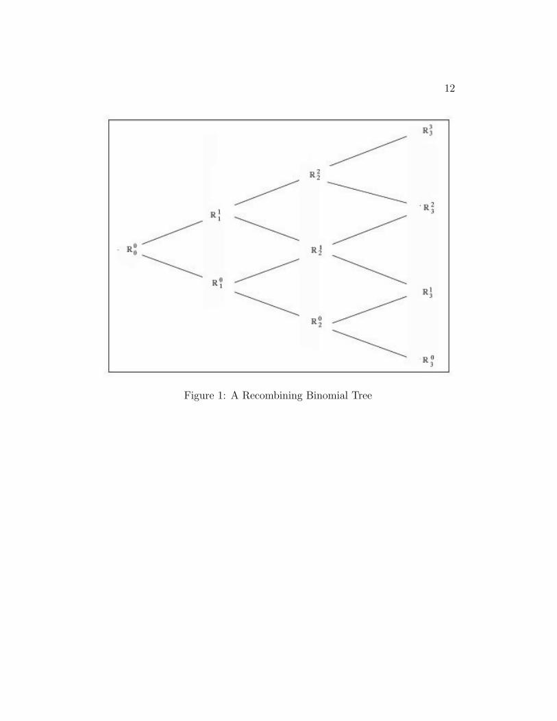
A binomial tree is a set of nodes with discrete spacing and times. At time

0 there is one root node with the current interest rate. From there it leads to

two other nodes. These represent the performance of the market with new

interest rates. As time goes on more and more possibilities can occur. In

a non-recombining model 2t nodes are created with each new time t. Every

node leads to two new unique possibilities. Recombining models are simpler

because there are only t+ 1 nodes at each time t. This is because two nodes

can point towards the same node in the next time step. Moving up then

down leads to the same node as moving down then up.

The forward measure is implemented through a Radon-Nikodym deriva-

tive process. A set of equations simplifies the problem from involving the

joint distribution of two random variables. This is the main advantage to

using the forward measure for derivative pricing.

3

2 Background

2.1 Bond Pricing Definitions

There are some common definitions used when pricing derivative securities.

These include zero-coupon bonds and the discount and interest rates with

volatility σ. Spot rates and yield rates are derived from interest rates. The

functions B(n, T ), D(n), and V (n) are also fundamental. Knowledge of all

of these is required to create our term structure.

Zero-coupon bonds are the simplest fixed income securities. Bought by

investors at a discount from their face value, they are bonds that have no

payoff until the end of their lifetime. The face value is the amount a bond will

be worth at some maturity time T . When a zero-coupon bond matures the

investor will receive one lump sum. By convention this value is $1. Given a

complete market any other derivative can be built using a portfolio composed

of only zero-coupon bonds of different maturity.

The interest rate R(n) is the rate at which the value of the zero coupon

bond increases over the step of time from n to n + 1. The value of future

interest rates R(n) : n > t where t is the current time are unknown; with

one exception. At the maturity of a bond, time T , a zero-coupon bond

will pay $1. So the interest rate from time T − 1 to time T is forced to

accommodate that. This special case is called the spot rate. A yield rate yn

is the average annual rate of return for a bond, while a yield curve is the set

4

of yield rates.

yn =n∏0

1

1 +R(n)(1)

Tied to the interest rate is the discount rate d(n), which is the inverse of

1 +R(n),

1 +R(n) =1

d(n)(2)

d(n) is used to know what price a bond had times previous to n. For instance,

at time T a zero coupon bond has a value of 1. d(T − 1) = 11+R(T−1)

is the

price of the bond at T − 1. It discounts the amount earned by R(n).

The value σn is the volatility of R(n) derived from historical data. In an

uncertain market this value is used as a parameter for estimation.

σ2n = E[Ri(n)2]− E[Ri(n)]2 ∀i known (3)

The function B(n, T ) is the price of a zero-coupon bond at time n with

maturity time T .

B(n, T )

B(n− 1, T )= B(n− 1, T )R(n) = B(n, T )d(n) (4)

Linked to this is the discount function D(n) which is the function used to

find the price B(0, T ) given B(n, T ).

D(n) =n∏i=1

d(i) (5)

5

The aptly named discount function defines how much the face value of a

future amount should be discounted for a fair price. This is easy when

R(n) : n ≤ T are known, but in an uncertain market an expectation of D(T )

must be used.

Lastly V (n) is the payoff function used to price other derivatives. Caps,

floors, and options are all common examples that pay an amount, fixed or

variable, when certain conditions occur. For instance, a cap may pay $0.01

every time R(n) is greater than some value S. V (n) would be the amount

earned by the derivative at time n. Finding the price of a derivative would

then require knowing what will occur with both the zero-coupon bonds and

the payoff function built on top of it.

6

2.2 Risk Neutral Measure

Arbitrage is a trading strategy that invests $0 and has a positive expected

return. Such practices are not desirable and cannot be found in complete

markets. As such, the Fundamental Theorem of Asset Pricing states that

there is no arbitrage in a market if and only if there exists a risk-neutral

measure equivalent to the real life probability measure. Furthermore, the

market is complete if that measure is unique. Unlike the real life measure the

risk-neutral measure values all derivatives on their expected payoff regardless

of risk. In real life risky ventures assets tend to have greater expected rates

of return.

The risk-neutral pricing formula uses the money market account as its

numeraire. A money market account is equivalent to a long position in

the shortest maturity zero-coupon bond. The interest rate for the money

market account is thus the interest rate at time t for zero-coupon bonds with

maturity t+1. These are the bonds that mature in the upcoming time period

at the spot rate. Characterized by the risk-less return such bonds experience,

they are useful for finding a zero-coupon bond evolution. Unfortunately, a

problem occurs when dealing with derivatives.

Pricing for derivatives depends on taking the conditional expectation of

the product of the payoff and random discount functions. The joint distribu-

tion of both is required when pricing with the risk neutral measure. Pricing

7

the payoff function at time n is defined as:

Vn =1

D(n)En[D(m)V (m)] (6)

given the first outcomes where n ≤ m ≤ N and En is the conditional

expectation. This conditional expectation relies on the previous n outcomes.

Likewise, En would denote expectation where the expectant value depends

on the first n outcomes. The difference in notation is that in the latter

the outcomes do not need to be known. Our payoff and discount functions

D(m)V (m) rely only on m outcomes, but n need to be known to find the

expectation.

It is possible to avoid needing the joint distribution of D and V with

a change of measure defined by a Radon-Nikodym derivative. As a result

expectations under the new measure no longer rely on future discounts.

8

2.3 Forward Measure

A zero-coupon bond bought at t with maturity T+1 would earn almost the

same rates as a bond bought at t with maturity T . They give identical

returns until time T . It is only in the time T + 1 that a difference occurs,

which is called the forward rate. The forward rate f(n, T ) is the implicit rate

earned by holding a bond an extra time period.

f(n, T ) =B(n, T )

B(n, T + 1)(7)

which gives

B(n, T ) =1∏T−1

i=1 f(n, i)(8)

These rates, built by zero-coupon bonds, are the foundation of the forward

measure.

To price under the forward measure it will be necessary to change from

the risk neutral measure. To begin with let m be fixed with 1 ≤ m ≤ N ,

with N the highest year our model is carried out to. Our Radon-Nikodym

derivative is:

Zm,m =D(m)

B(0,m)(9)

With the use of Zm,m it is possible to define P∗m to be the m-forward

measure on our probability space Ω, where Ω is the set of all possible out-

comes for market movements. Letting P denote the risk neutral-measure on

9

Ω that assigns a probability to each event, we define

P∗m(w) = Zm,m(w)P(w) ∀w ∈ Ω (10)

P∗m is a probability measure absolutely continuous with respect to the risk

neutral probability measure P. We can verify that P∗m(Ω) is assigned a

probability of 1 because EZm,m = 1.

P∗m(Ω) =∑w∈Ω

P∗m(w) =∑w∈Ω

Zm,m(w)P(w) = EZm,m =1

B(0,m)EDm = 1

(11)

The relationship between zero-coupon bond prices and the discount func-

tion allows that:

B(n,m) = En[D(m)

D(n)] =⇒ D(n)B(n,m) = En[D(m)] (12)

Which in turn can define

Zn,m = En[Zm,m] =D(n)B(n,m)

B(0,m)(13)

Thus, under our previous definition of V coupled with the following

Em[Vm] = E[Zm,mVm] (14)

10

we can use the m-forward measure P∗m to get:

Emn [Vm] =

VnB(n,m)

(15)

In summary, this is the expectation of the payoff function at time m when

Vm relies on the first m outcomes and the first n are known. It is defined by

zero coupon bond prices maturing at time m. For all n this is the forward

price of the security.

11

3 The Ho-Lee Model

3.1 General Model

To implement the pricing of securities under the forward measure the discrete

Ho-Lee model was chosen. It is a simple recombining binomial model derived

by market volatility. At each time node the interest rate Rn may step up

or down to a new node. The discount function D can therefore be found by

tracing paths from node to node and finding the interest rates; which are

defined as follows:

Rcn = an + bn · c (16)

Where an and bn are calibration constants derived from data and c is the

number of ‘up’ steps taken in that path. Developed by T.S.Y. Ho and S.B.

Lee in 1986 [3], this was the first model to find single period risk-less returns

required to match bond prices.

Nodes are the basis of the tree and each represents both a point in time

and a link to its parent and children nodes. Figures 1 and 2 are visual

representations of the model.

12

Figure 1: A Recombining Binomial Tree

13

Figure 2: A Non-Recombining Binomial Tree

14

3.2 Drawbacks

There have been many variations and elaborations on the Ho-Lee model.

This is because it has a few shortcomings. Most of these stem from being

too simple a model without the flexibility to accurately reflect the market.

The model has only one parameter, volatility σ, which is assumed to be

constant. The volatility for each period is estimated using historical data, but

there is no mechanism for changing the values as the model goes on. Newer

models can have both multiple factors and volatility that changes over time.

Static volatility is a problem computationally because that is the basis for

bn. If the yield curve drifts over time there will be a larger volatility. Coupled

with a large n, the resulting interest rates may very well be negative. This

is because the Ho-Lee model builds a symmetric term structure.

15

3.3 Alteration

The basic structure of the Ho-Lee model was used but slight modifications

were required. The algorithm described in detail in section 4 is used to

derive interest rates from historical data. This required continuously com-

pounded interest rates in the calculations and output. Standard implementa-

tion called for a discrete time model. It is possible to transform continuously

compounded rates to annual rates by knowing the relationship:

eR∞(n) = 1 +R(n) (17)

Where R∞(n) is the continuously compounded rate, and R(n) is our standard

definition for the interest rate.

Converting from continuously compounded to annual interest rates results

in a new problem. The rates are converted to the an and bn’s required by the

Ho-Lee model in equation 16. The problem lies in the bn·c. In continuous time

the system is built symmetrically, with the vertical distance between nodes

the same (see Figure 1.) This value was equal to bn. The transformation into

discrete time, however, made each step size slightly greater than the last.

(e−a∞+b∞ − 1)− (e−a∞ − 1) < (e−a∞+2b∞ − 1)− (e−a∞+b∞ − 1) (18)

16

Figure 3: Differences in Translation

17

Figure 3 illustrates the problem. On the left are the derived an and bn

values found from continuously compounded rates. On the right are the

translated values into their discrete time equivalents. ∆ represents the dif-

ference shown in equation 18. Therefore, the differences between nodes R02,

R12, and R2

2 are no longer constant.

This was the only way to get closed form solutions for the interest rates.

So the Ho-Lee model was altered as described. The modular nature of the

model also allows for this change to be undone easily.

18

4 Extracting Interest Rates

For the model to be useful in predicting bond prices we require a methodology

for choosing sets of an and bn. This was started by using Agca and Chance’s

[6] method for deriving rates for Ho-Lee models. Their approach requires

working with continuous compounding. According to the authors, this is the

only way to achieve a closed form solution.

This approach requires two inputs to estimate interest rates from histori-

cal information. First we need the volatility of spot rates at each t ≤ N . As

this is the Ho-Lee model, these values are constant. Second is the time zero

zero-coupon bond prices for each t ≤ N + 1. Both these inputs can be found

using historical zero-coupon bond yield curves.

The algorithm described revolves on iteratively solving systems of equa-

tions. As such, the following values are found:

b(n) = 2σn (19)

an + nB(n) = lnQn

2nB(0, n+ 1)(20)

=⇒ an = lnQn

2nB(0, n+ 1)− 2nσn (21)

Qn = e−Pn−1

j=0 aj+Bjj

n∏j=1

[1 + e2Pj−1

k=0 σn−k ] (22)

It is easily verifiable to see this algorithm is accurate by passing the

outputs an and bn to the model and retrieving the same time zero-coupon

19

bond prices as entered.

The programmed implementation starts by reading in a set of N yields.

Since the Ho-Lee model assumes constant volatilities they could be read in

once along with the yields. A two-pass function derives its own values for

the mean and volatility. Afterwards the yields can give the B(0, t) prices for

all t ≤ N . Similarly a0 is defined as 1B(0,1)

. From there Qj for j ≤ N is found

by using nested loops to follow the above algorithm. The relevant output aj

is stored in a new array. From here our sets of an and bn can be output to a

file or passed to the Ho-Lee model.

20

5 Calibration

Now that methods for pricing derivatives given interest rates and extracting

interest rates from historical data have been established, the next step is to

calibrate the data so as to have an accurate model of the real world. This

can be approached a few different ways.

First, the Ho-Lee model depends on volatility. It is possible to use one

constant volatility σ for each time n or a variable σn can be used. Since these

values are derived from data the set, σn gives more flexibility to the model.

This leads to a more accurate representation.

Volatility is defined in Eq. (3). The practical method to get this value for

a large population is as follows:

σ =

√√√√ 1

N − 1

N∑i=1

(xi − x)2 (23)

x is defined as the mean of the N xi historical samples. This method is

iterated for each time n until a set of σn is found. As mentioned before, the

Ho-Lee model is too simple to calibrate on a large data set. There is a limit

to what volatility will give non-negative interest rates, which goes down as n

increases. The derived interest rates are weighted to center around the mean

of spot rates. bn = 2σn gives the size of the spread between nodes. If the

spread is sufficiently large, or mean is sufficiently low, negative interest rates

will result.

21

For instance, take a4 = -.01, bn = 2σ = .03.

R03 = −.01, R1

3 = .02, R23 = .05, R3

3 = .08 (24)

The expected R3 has a perfectly valid value between .02 and .05, despite

having a negative R03. The model has no corrections for this type of behavior.

22

6 Passing Information

There have been two distinct processes created to price under the forward

measure. The first extracts rates from raw data, and the second extracts

prices given rates. These communicate by passing csv (comma separated

variable) files.

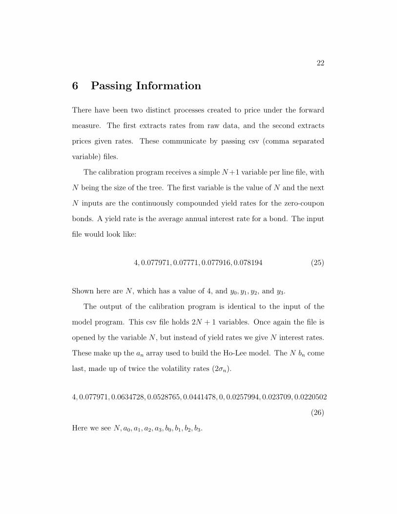
The calibration program receives a simple N+1 variable per line file, with

N being the size of the tree. The first variable is the value of N and the next

N inputs are the continuously compounded yield rates for the zero-coupon

bonds. A yield rate is the average annual interest rate for a bond. The input

file would look like:

4, 0.077971, 0.07771, 0.077916, 0.078194 (25)

Shown here are N , which has a value of 4, and y0, y1, y2, and y3.

The output of the calibration program is identical to the input of the

model program. This csv file holds 2N + 1 variables. Once again the file is

opened by the variable N , but instead of yield rates we give N interest rates.

These make up the an array used to build the Ho-Lee model. The N bn come

last, made up of twice the volatility rates (2σn).

4, 0.077971, 0.0634728, 0.0528765, 0.0441478, 0, 0.0257994, 0.023709, 0.0220502

(26)

Here we see N, a0, a1, a2, a3, b0, b1, b2, b3.

23

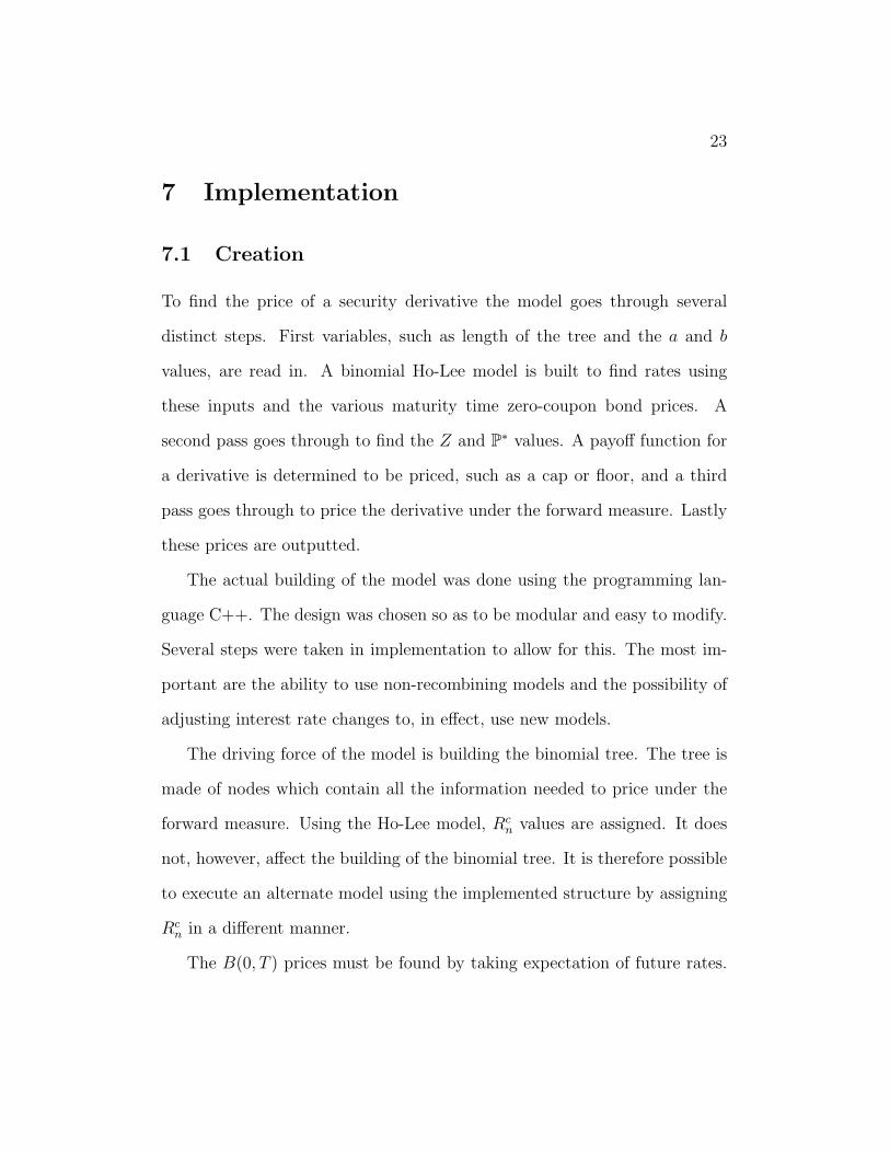
7 Implementation

7.1 Creation

To find the price of a security derivative the model goes through several

distinct steps. First variables, such as length of the tree and the a and b

values, are read in. A binomial Ho-Lee model is built to find rates using

these inputs and the various maturity time zero-coupon bond prices. A

second pass goes through to find the Z and P∗ values. A payoff function for

a derivative is determined to be priced, such as a cap or floor, and a third

pass goes through to price the derivative under the forward measure. Lastly

these prices are outputted.

The actual building of the model was done using the programming lan-

guage C++. The design was chosen so as to be modular and easy to modify.

Several steps were taken in implementation to allow for this. The most im-

portant are the ability to use non-recombining models and the possibility of

adjusting interest rate changes to, in effect, use new models.

The driving force of the model is building the binomial tree. The tree is

made of nodes which contain all the information needed to price under the

forward measure. Using the Ho-Lee model, Rcn values are assigned. It does

not, however, affect the building of the binomial tree. It is therefore possible

to execute an alternate model using the implemented structure by assigning

Rcn in a different manner.

The B(0, T ) prices must be found by taking expectation of future rates.

24

Pricing derivatives under the forward measure does not take the origin of the

rates into account, just that they exist. Any model may be used to output

rates.

25

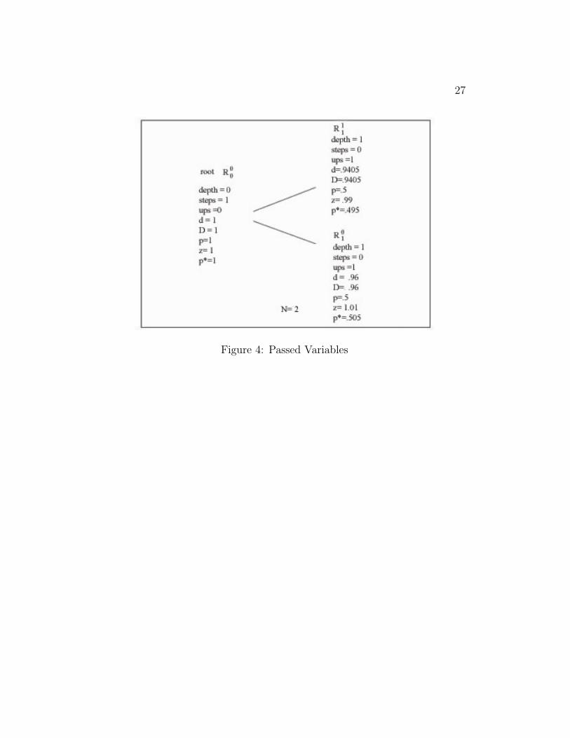
7.2 Data Variables

The first data item to be stored is the depth of a node, which represents its

place in time. The first node at time 0, or the root, has a depth value of

zero. Each step along the path, representing an increase in time, increments

the depth by a value of one. Tied to that is the number of time steps left

until the tree is complete. This is of use when building the tree. This value

could also be derived knowing the current node depth and total depth of

the tree, N . Particularly important for the Ho-Lee model is the counter for

‘up’ movements. Each node (barring the last set) has two children, one that

represents an up movement in interest rates, and one down. This is what the

Ho-Lee model uses to create interest rates.

Variables are created to store data derived from interest rates. Both the

discount rate d(n) and discount function D(n) are stored for each node. The

risk-neutral probabilities are kept as well, to find B(0, t).

Last are the values associated with pricing under the forward measure.

The probability of reaching that node under the forward measure P∗ and

Z, its Radon-Nikodym derivative with respect to the risk neutral measure

P. These are derived as explained above, with Z a function of the discount

function with the relevant node and the time zero zero-coupon bond with

maturity N . P∗ is the product of Z and the probability of reaching the

node under the risk-neutral measure. The programming structure allows the

odds of an up or down movement to be changed, although as in Agca[6]

we assume risk-neutral probabilities of 12. The real risk-neutral probabilities

26

may be slightly different to be consistent with the absence of arbitrage. The

flexibility provided by the model parameters compensates for this assumption

and return proper results.

27

Figure 4: Passed Variables

28

7.3 Functions

Upon creation of a node, a function is called to return the derived interest

rate. This is where the program form may be used for different models. A

different value function can be substituted in, thus altering the term struc-

ture. Once the value is retrieved, whatever it may be, the inverse is taken

to find the discount rate d(n) for that year. The discount function, D(n) as

defined before, is the product of all discount rates in a particular path. That

rate is also stored along each node in a path and can be derived by multiply-

ing the parent node’s discount function by the current node’s discount rate.

To this effect, and in the act of building the tree, the pointers to the parent

and children nodes are stored. With this the time zero zero-coupon bond

price with a maturity of the node depth can be found, which is stored in an

array of size N .

The program reads in the N , an, and bn values required to build a Ho-

Lee tree. If a different model wishes to be used the form of the input file

would be different. A new root is created with an interest rate of a0 and

probability of 1. The price of the time zero zero-coupon bond would simply

be it’s discount rate. Until the the proper depth is reached, the root and all

following nodes create children. They pass on their discount function and the

new nodes call an interest rate value function. Here the continuous interest

rates are transformed to create a discrete tree as explained above. Using that

information the tree finds the relevant B(0, n). This is done by summing the

product of the current nodes discount rate and it’s parents discount function

29

with the risk neutral probabilities that this outcome would occur.

Now that we have both the discount function for each path leading to

a node and the time zero zero-coupon bond price B(0, n) for each maturity

date the Z and P∗ values can be computed. A recursive passthrough, starting

at the root and passing on to its children, begins. Finally, a second set of

inputs decides which derivative security should be priced. Although only a

few securities are currently created, the comparison process is also modular.

By setting new constraints to compare the interest rate at each node to

some value any security can be created. The payoff function is given a value

according to this, and a recursive pass through can price it using the P∗

probabilities.

30

8 Results

8.1 Estimated Rates

To estimate interest rates from historical data, 100 yield curves were used.

The selection started in 1990 and chose every 5th business day, going well

into 1992.

N y0 y1 y2 y3

11 0.077971 0.07771 0.077916 0.07819411 0.077771 0.077765 0.078179 0.07862311 0.079992 0.080278 0.080764 0.08115411 0.081011 0.081766 0.082487 0.08301611 0.081519 0.082646 0.083407 0.08384411 0.080255 0.081052 0.081723 0.082211 0.080889 0.082611 0.083483 0.08395211 0.081909 0.083448 0.084479 0.08508911 0.08379 0.085435 0.086192 0.086457

Table 1: Input to Estimate Rates

N a0 a1 a2 b0 b1 b2

11 0.077971 0.0634728 0.0528765 0 0.0257994 0.02370911 0.077771 0.0637828 0.0535555 0 0.0257994 0.02370911 0.079992 0.0665878 0.0562845 0 0.0257994 0.02370911 0.081011 0.0685448 0.0584775 0 0.0257994 0.02370911 0.081519 0.0697968 0.0594775 0 0.0257994 0.02370911 0.080255 0.0678728 0.0576135 0 0.0257994 0.02370911 0.080889 0.0703568 0.0597755 0 0.0257994 0.02370911 0.081909 0.0710108 0.0610895 0 0.0257994 0.02370911 0.08379 0.0731038 0.0622545 0 0.0257994 0.023709

Table 2: Estimated Rates

31

Only a truncated version is shown. A full 12 variable 100 line file was ac-

tually input and a 23 variable file was output. So far the results are straight-

forward and unsurprising. a0 is the root node, and is therefore the only node

at time 0. This correlates to the value of b0, which is 0. Also, it is evident

that all bn are constant, regardless of time. This is one of the drawbacks of

the Ho-Lee model. It is caused by assuming a constant volatility across time.

32

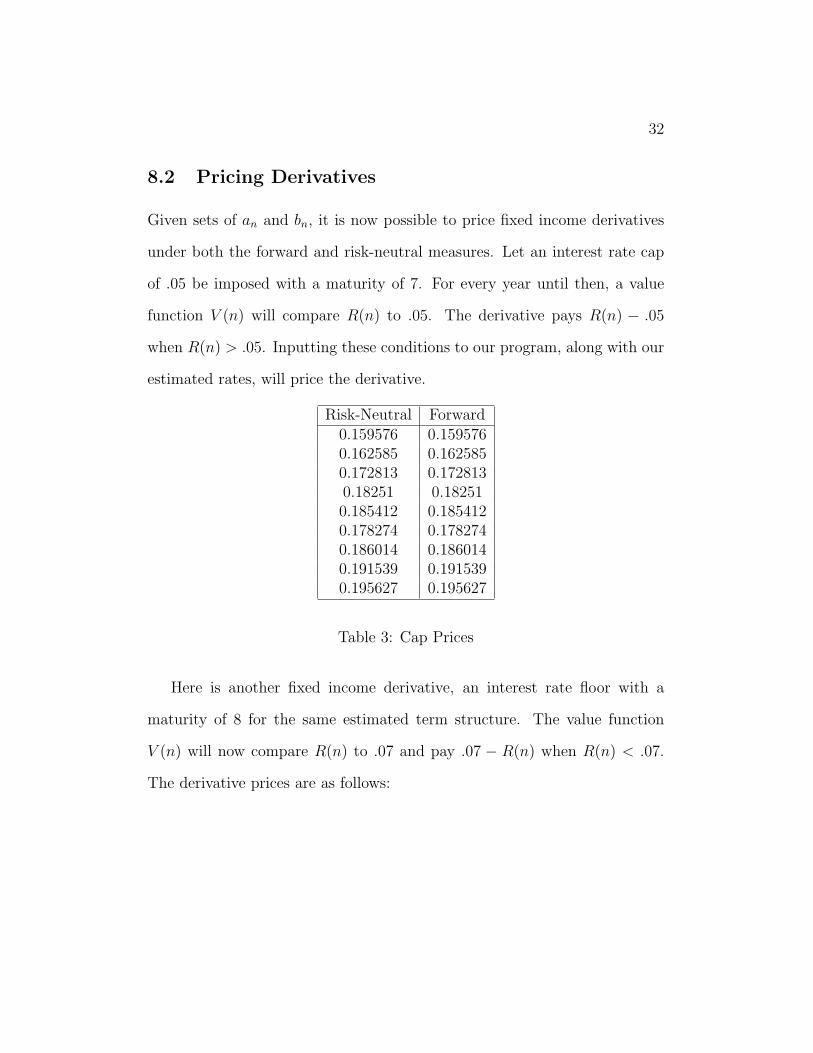
8.2 Pricing Derivatives

Given sets of an and bn, it is now possible to price fixed income derivatives

under both the forward and risk-neutral measures. Let an interest rate cap

of .05 be imposed with a maturity of 7. For every year until then, a value

function V (n) will compare R(n) to .05. The derivative pays R(n) − .05

when R(n) > .05. Inputting these conditions to our program, along with our

estimated rates, will price the derivative.

Risk-Neutral Forward0.159576 0.1595760.162585 0.1625850.172813 0.1728130.18251 0.182510.185412 0.1854120.178274 0.1782740.186014 0.1860140.191539 0.1915390.195627 0.195627

Table 3: Cap Prices

Here is another fixed income derivative, an interest rate floor with a

maturity of 8 for the same estimated term structure. The value function

V (n) will now compare R(n) to .07 and pay .07 − R(n) when R(n) < .07.

The derivative prices are as follows:

33

Risk-Neutral Forward0.0210254 0.02102540.0195019 0.01950190.0159325 0.01593250.0127138 0.01271380.0122266 0.01222660.0138367 0.01383670.011993 0.0119930.0105975 0.01059750.0102725 0.0102725

Table 4: Floor Prices

Pricing under both measures gives the same result, as is expected. The

surprising result is that there is no notable change in computational speed

between methods. This is because our model is required to calculate the

B(0, n) prices, regardless.

By assigning possible values and probabilities to the discount function

D(n) the binomial implementation of the Ho-Lee model avoids the difficulties

involved with a random D(n). If D(n) were treated as a true random variable

with some distribution, the joint distribution between D and V would be

required for risk-neutral valuation.

The forward measure also has the advantage in pricing when B(0, n)

prices are readily available.

34

References

[1] Geman, H., El Karoui, N., and J. C. Rochet “Changes of Numeraire,

Changes of Probability Measure and Option Pricing.”Journal of Applied

Probability 32, 1995, 443-458.

[2] Hull, J., and A. White “Numerical Procedures for Implementing Term

Structure Models I: Single-Factor Models.” Journal of Derivatives Fall,

1994, 716.

[3] Ho, T. S. Y. and S-B Lee “Term Structure Movements and Pricing

Interest Rate Contingent Claims.” The Journal of Finance 41, 1986,

1011-1030.

[4] Ji, Chuanshu “Lecture Notes on Discrete-time Finance.” 1998.

[5] Rogers, L. C. G. “The Origins of Risk-Neutral Pricing and the Black-

Scholes Formula.” Risk Management and Analysis 2, 1998, 81-94.

[6] Agca, Senay and Don M. Chance “Two Extensions for Fitting Discrete

Time Term Structure Models with Normally Distributed Factors.” 2003.

[7] Roman, Jan R. M. “Lecture Notes in Analytical Finance II.” Malardalen

University, 2005.

[8] Musiela, Marek and Marek Rutkowski, Martingale Methods in Financial

Modelling. Springer, 1997.

35

[9] Kwok, Y. K., Mathematical Models of Financial Derivatives. Springer

Finance, 1998.

[10] Shreve, Steven, Stochastic Calculus for Finance I: The Binomial Asset

Pricing Model. Springer Finance, 2003.