Federal Reserve Bank of Dallas Globalization and Monetary Policy Institute

Working Paper No. 187 http://www.dallasfed.org/assets/documents/institute/wpapers/2014/0187.pdf

Pricing-to-Market and Optimal Interest Rate Policy*

Dudley Cooke

University of Exeter

August 2014

Abstract I study optimal interest rate policy in a small open economy with consumer search in the product market. When there are search frictions, firms price-to-market, with implications for the design of monetary policy. Country-specific shocks generate deviations from the law of one price for traded goods which monetary policy acts to stabilize by influencing firm markups. However, stabilizing law of one price deviations results in greater fluctuations in output. JEL codes: E31, E52, F41

* Dudley Cooke, Department of Economics, University of Exeter, Streatham Court, Rennes Drive, Exeter EX4 4PU. United Kingdom. 44-0-1392-726257. d.cooke@exeter.ac.uk. I thank Tatiana Damjanovic and Christian Siegel for discussions.The views in this paper are those of the author and do not necessarily reflect the views of the Federal Reserve Bank of Dallas or the Federal Reserve System.

1. Introduction

Pricing-to-market by exporting firms, and induced deviations in the law of one price, have

important implications for the design of monetary policy in open economies.1 In this paper, I

study optimal interest rate policy with consumer search in the product market and pricing-to-

market behavior by firms. I consider consumer search for two reasons. First, the frictions

induced by search costs have been shown to help match key statistics on fluctuations in

international relative prices.2 Second, search provides a simple, micro-founded explanation

for endogenous markups and equilibrium price dispersion across countries.

I develop a small open economy model where consumers actively search to reduce the price of

the goods they consume. This allows for short-run deviations from the law of one price, and

because search takes time, its opportunity cost is measured in terms of foregone labor income.

Consumption purchases are subject to a cash-in-advance restriction. The opportunity cost

of search is therefore adjusted for the cost of holding money. In this case, the path of the

nominal interest rate influences the markup charged by the firm, in addition to allocations

and international relative prices.3

In the open economy, by using the interest rate to influence the terms of trade, a policymaker

can raise the level of home consumption, for a given level of output. Absent search frictions,

it is optimal to raise (or lower) the nominal interest rate in response to shocks depending

on the elasticity of substitution between home and foreign goods - the trade elasticity - and

the intertemporal elasticity of substitution in consumption. Because optimal policy can be

1Empirical evidence points to pricing-to-market being strong and persistent. For example, see Atkeson

and Burstein (2008) and Gopinath and Itskhoki (2010).2Neither real business cycle models nor sticky price models have been able to account for movements in

international relative prices observed in the data. See Backus et al. (1995) and Chari et al. (2002).3I use a cash-in-advance constraint for simplicity. In general, any transactions technology will mean that

the interest rate influences the markup due to the nature of the search frictions I consider.

2

expressed solely in terms of output - with no additional role for the exchange rate - in a

special case, when the two elasticities are equal, the interest rate is invariant to fluctuations

in the business cycle.4

When there are search frictions in the product market, it is optimal for the interest rate

to respond to shocks, even under the special case just described. Moreover, the interest

rate can also be written as a function of deviations from the law of one price for the home

good. When the home good is relatively expensive in the domestic market - and the home

currency is overvalued - interest rates are raised, because a higher interest rate reduces the

desired markup, forcing firms to charge a lower price for their product. However, because an

overvalued currency is also consistent with a drop in external demand, by focusing exclusively

on law of one price deviations, monetary policy generates greater fluctuations in output.

Deviations from the law of one price for the home good are sufficient to explain interest rate

policy in the special case because home consumer search for the foreign good is exogenous

from the perspective of the policymaker. However, in general, the interest rate reacts to

deviations from the law of one price for the foreign good and the mass of shoppers sent out

by households to search for (home and foreign) goods. In this case, simple expressions for

interest rate policy are unavailable, and I undertake a numerical exercise to determine how

law of one price deviations add to fluctuations in the business cycle under optimal policy.

The results I present can be compared to those that study monetary policy in models of

pricing-to-market based on sticky-prices.5 Monacelli (2005) argues that optimal policy

under commitment requires the stabilization of law of one price deviations for imported goods

using a small open economy model. Engel (2011) studies the role of currency misalignments

4The reasoning behind this result is very standard, and is similar in spirit to the analysis of Benigno and

Benigno (2003), albeit with flexible prices.5In models with nominal rigidities, pricing-to-market is the result of fluctuations in the nominal exchange

rate and sticky local prices.

3

(defined as a weighted average of deviations from the law of one price over home and foreign

goods) in a two-country setting, and shows why policy should account for exchange rate

movements (in addition to inflation and an output gap) under cooperation. In this paper,

I find that optimal interest rate policy acts to smooth-out deviations from the law of one

price, and hence should also be concerned with currency misalignments.

This paper is also related to research on product search in dynamic general equilibrium

models. The rationale for law of one price deviations I adopt is based on the two-country

business cycle model of Alessandria (2009). However, in the closed economy, Head et al.

(2012) embed product search into a search-theoretic model of money with the result that

money shocks are neutral but prices adjust sluggishly, and Kaplan and Menzio (2013) develop

a model with self-fulfilling fluctuations that result from the interaction of product search and

search and matching in labor markets.6 In the open economy, Liu and Shi (2010) use a

monetary search model to study policy coordination when there are deviations from the law

of one price driven by a cross-country differential in money growth.

A final point is that open economy RBC models with complete international asset markets

and productivity shocks generate procyclical terms of trade.7 Corsetti et al. (2008) have

shown how incomplete asset markets coupled with a low trade elasticity can overturn this

result, but recent research has pointed to alternative channels, via induced movements in

the labor wedge arising from home production (Karabarbounis, 2014), or search frictions in

product markets (Bai and Rios-Rull, 2013). In this paper, I do not attempt to explain which

friction is more relevant for generating countercyclical terms of trade, rather, I demonstrate

6Arseneau et al. (2014) study optimal fiscal and monetary policy with search frictions based on long-term

relationships.7The opposite appear to hold in the data. The raw correlation between the terms of trade an output is

reported in Heathcote and Perri (2002) as being −0.24. Similar values are reported in Alessandria (2009)

and Bai and Rios-Rull (2013). Evidence based on vector autoregressions is presented in Enders and Muller

(2009).

4

why consumer search in the product market is important for the conduct of monetary policy

in the open economy.

The remainder of the paper is organized as follows. In section 2, I develop a small open

economy monetary model with consumer search in the product market. I consider optimal

stabilization policy in section 3. Section 4 concludes.

2. Model

I consider a two-country economy. The home country is populated by a continuum of house-

holds of total measure 1 and the foreign country is populated by a continuum of households

of total measure ω. Thus, ω is the population size of the home country relative to the foreign

country. In both countries households maximize lifetime utility, where period utility is a

function of consumption and the mass of workers and shoppers. In each country, firms

supply an identical good produced using labor.

In what follows, I focus the exposition of the model on the home country, with the under-

standing that analogous expressions hold for the foreign country. Consumption, output, and

the nominal price of the home/foreign output are denoted with h/f -subscripts. Asterisks

denote foreign country variables.

2.1. Households

Households have the following intertemporal utility function,

U = E0

∞∑t=0

βt [u (ct)− κt (lt + st)] ; ct =[(1− χ)1/ξ c

(ξ−1)/ξh,t + χ1/ξc

(ξ−1)/ξf,t

]ξ/(ξ−1)(1)

The variable ct is a consumption aggregate over the home (ch,t) and foreign (cf,t) good, lt is

total labor supplied for production, and st ≡ sh,t + sf,t is the measure of shoppers (of which

there are sh,t/sf,t) searching for the home/foreign . The parameter ξ > 0 is the elasticity of

5

substitution between home and foreign goods (the trade elasticity) and χ = αω/ (1 + ω) is a

weight placed on the foreign good in consumption, where α is a measure of trade openness.

The disutility of shopping and labor are assumed to be linear and the variable κt is a shock to

the marginal disutility of labor as in Hall (1997). With search frictions this shock generates

countercyclical movement in the terms of trade. Since without search the shock mimics

shocks to productivity, it provides a simple benchmark from which to asses the importance

of search-based pricing-to-market for optimal monetary policy.8

Households start period t with nominal wealthWt, receive monetary transfers Tt, and choose

money holdings Mt, and nominal bond holdings Bt, that pay RtBt one period later.9 The

gross nominal interest rate at date t is Rt. Households also buy At+1 units of home currency

state-contingent nominal securities. Each security pays one unit of money at the beginning

of period t + 1 in a particular state where Qt,t+1 is the beginning of period t price of these

securities normalized by the probability of the occurrence of the state. In the asset market

at the beginning of period t households face the constraint,

Mt +Bt + EtQt,t+1At+1 − Tt ≤ Wt (2)

After leaving the asset market households enter the goods and labor markets. Consumers

search to reduce the price of home and foreign goods. With probability z each shopper gets

a price quote from only one (1) firm and with probability (1− z) they get price quotes from

two (2) firms. The cumulative distribution of the lowest price drawn by a shopper is,

J(pi) = zF (pi) + (1− z)[1− (1− F (pi))

2] (3)

8For a quantitative analysis of this type of shock, without search frictions, see Holland and Scott (1998).

Nakajima (2005) presents a microeconomic foundation for the shock, which, more generally, should also be

viewed as part of the labor wedge, as stressed in Chari et al. (2007).9Each period is divided into two sub-periods, with the asset market operating in the first sub-period and

the goods market in the second.

6

where pi ∈[pi, pi

]and F (pi) is the cumulative density function of price quotes for goods

i = h, f in the economy. With a reservation-price pi ≥ pi, a shopper buys the good,

with probability J(pi), at the expected price of P (pi). Thus, in period t, the amount the

shopper expects to buy is P (pi,t) J(pi,t) =∫ pi,t0

pidJ(pi). The household sends si,t agents

to shop, and since the total amount of good purchased is equal to the number of shopping

trips, consumption is ci,t = si,tJ(pi,t).

A fraction 1vt

of the households consumption purchases must be made with money such that

the following cash-in-advance constraint is satisfied,

Ωt

vt≤Mt (4)

where Ωt ≡ sh,t∫ ph,t0

ph,tdJ(ph,t) + sf,t∫ pf,t0

pf,tdJ(pf,t). Households also receive labour in-

come, Wtlt, where Wt is the nominal wage rate, and dividends from all firms, denoted Φt.

The nominal wealth at the beginning of period t+ 1 is,

Wt+1 = Mt +RtBt + At+1 − Ωt +Wtlt + Φt (5)

The households problem is to choose Bt, At+1,Mt, lt, si,t, pi,t∞t=0 to maximize, (1), subject

to (2)-(5). For securities, we get standard expressions, albeit evaluated at the reservation

price.

u′ (ct)

pt= R′tEt

[βu′ (ct+1)

pt+1

Rt+1

R′t+1

]and Qt−1,t = β

(u′ (ct+1) /pt+1)(Rt+1/R

′t+1

)(u′ (ct) /pt) (Rt/R′t)

(6)

where R′t = 1+(Rt − 1) /vt and EtQt,t+1 = 1/Rt. When vt = 1, then R′t = Rt, and equation

(4) coincides with the standard cash-in-advance constraint. As vt →∞, the cash constraint

becomes irrelevant, R′t = 1, and the model reduces to a real model. The choice of labor and

search effort generates the following conditions.

κtu′ (ct)

=Wt

ptR′tand

Wt

R′t= [pi,t − P (pi,t)] J(pi,t) (7)

7

The first condition captures the labor-leisure trade-off where the intratemporal marginal rate

of substitution between leisure and consumption equals the real wage adjusted for the cost of

holding money. The second condition captures the trade-off between sending out (1/J(pi,t))

more shoppers, with the expectation of paying P (pi,t) for a unit, and receiving a lower price.

Note that the opportunity cost of search is measured in terms of foregone labor income, and

is also adjusted for the cost of holding money.

Finally, the choice over home and foreign goods is characterized by,

cf,tch,t

=

(χ

1− χ

)(ph,tpf,t

)ξand p1−ξt = (1− χ) p1−ξh,t + χp1−ξf,t (8)

We can also generate the demand functions for home and foreign goods in terms of overall

consumption, ch,t = (1− χ) (pt/ph,t)ξ ct and cf,t = χ (pt/pf,t)

ξ ct, respectively. As ξ → 0 we

recover the Cobb-Douglas case with unit-elastic demand functions. It is worth restating

that conditions (6)-(8) are all in terms of reservation prices, as these determine marginal

decisions.

2.2. Firms

In each country, there are many firms producing a country-specific good. Each firm has

technology, yh,t + y?h,t = lh,t + l?h,t. Home (foreign) households send sh,t (s?h,t) shoppers to

search for the home good. The total profit for a firm serving both markets is denoted φt,

and I write this as,

φh,t + φ?h,t = (ph,t −Wt) dh,t +(etp

?h,t −Wt

)d?h,t (9)

where dh,t/q = 1 + ς [1− F (ph,t)] and d?h,t/q = 1 + ς[1− F

(p?h,t)]

are the demand curves

per-shopper faced by the firm (in the home and export market) and ς ≡ 2 (1− q) /q.10 The

10A fraction q/ [q + 2 (1− q)] of consumers get one (1) quote, and a fraction 2 (1− q) / [q + 2 (1− q)] get

two (2) quotes. Combining these expressions, the probability that a shopper purchases from a firm charging

pt is, q (pt) ≡ q + 2 (1− q) [1− F (pt)] / (2− q) for pt ≤ pt and q (pt) = 0 if pt > pt. The demand curve

per shopper is then, d (pt) ≡ q (pt)× (2− q).

8

firm maximizes profit per-shopper, choosing ph,t and p?h,t, with reservation prices, ph,t and

p?h,t, and input costs Wt given, such that, yh,t = dh,t and yh,t = d?h,t. The maximum price a

firm can charge in the domestic (export) market is the consumers local-currency reservation

price so the solutions to the firms problems imply the following price distributions,

F (ph,t) = 1− 1

ς

(ph,t − ph,tph,t −Wt

)and F

(p?h,t)

= 1− 1

ς

(p?h,t − p?h,tp?h,t −Wt/et

)(10)

where F(ph,t

)= 0 and F

(p?h,t

)= 0 determine the lower point on the price distributions.

Notice that firms are indifferent between charging any price on pi ∈[pi, pi

]and because

firms can be viewed as randomizing, the both price distributions, F (pi,t), are continuous.

2.3. Equilibrium

Solving the model involves finding the reservation price using the search conditions in (7)

along with (10).11 A key feature of the model is that (7) contains the nominal interest rate.

Although this is standard feature of a cash-in-advance model without search, with consumer

search, this means that the interest rate also affects firms behavior. To see why, consider

the following conditions, that describe the distribution of prices.

ph,t =

[1 +

(1

1− z

)1

R′t

]Wt and p

h,t=

[2 (1− z)

2− z

]Wt +

(z

2− z

)ph,t (11)

with average price P (ph,t) = ph,t−Wt/R′t and where J(ph,t) = 1. The square brackets of the

first expression in (11) is the markup charged by a firm over the marginal cost of production,

Wt. The markup is decreasing in the nominal interest rate. An analogous condition holds

for the foreign good, albeit adjusted for the exchange rate, et, which enters via firm profits.

The export price is therefore given by, etp?h,t =

[1 +

(1

1−z

) ( etW ?t

Wt

)1R?′

t

]Wt. Now we see that

the law of one price need not hold. I define additional variables that track deviations from

the law of one price, ψh,t ≡ etp?h,t/ph,t and ψf,t ≡ etp

?f,t/pf,t, for the home and foreign good,

respectively.

11The details of this are relegated to Appendix A.1.

9

Now consider the efficiency condition for bonds’ holdings by foreign consumers, which can be

written as, Qt−1,tu′ (c?t−1) /et−1p?t−1 = βu′ (ct−1) /etp

?t . Combining this with the equivalent

condition for home consumers, the risk-sharing condition is,

qt = u′ (c?t ) /u′ (ct) (12)

where qt ≡ etp?t/pt is the real exchange rate, expressed in terms of reservation prices. Fi-

nally, I also derive resource (output and shopping) constraints. Output is equal to home

consumption plus exports, ch,t + ωc?h,t, and using the demand conditions above,

yt = (1− χ)

(ptph,t

)ξct + χ?ω

(p?tp?h,t

)ξ

c?t (13)

where χ = αω/ (1 + ω), χ? = α/ (1 + ω), and α = α?. This condition is standard except

insofar as deviations from the law of one price for home goods affect export demand. The

shopping constraint is given by, st = sh,t + sf,t, and so,

st = (1− χ)

(ptph,t

)ξct + χ

(ptpf,t

)ξct (14)

where yi,t = si,t. Thus, shopping depends on home consumption only. From here on, I

assume the home economy is small in the sense that ω → ∞.12 In this case, we can write

the foreign economy resource constraints as, y?t = c?t = s?t , which is exogenous from the

perspective of the home economy.

3. Optimal Monetary Policy

In the following sections I characterize optimal monetary policy under commitment. Each

monetary authority sets its interest rate and injects money in the economy through lump-

12In this case, there is home-bias in consumption in the sense that the home country is small and the limit

of the ratio of expenditure share on home goods to population share is not equal to one. For example, see

Faia and Monacelli (2008).

10

sum transfers.13 I assume throughout that the foreign economy is at a steady-state with a

zero nominal interest rate. In the absence of foreign shocks, such a policy is optimal under

commitment, and this allows me to focus on the policy problem for the home economy.

3.1. International Relative Prices

I first make some definitions which help explain the role of international relative prices in

determining policy decisions. I begin by denoting ρt ≡ pf,t/ph,t and ρ?t ≡ p?f,t/p?h,t for relative

prices within each economy. It is worth stressing that these variables are not the terms of

trade. The terms of the trade for the home economy, for example, are given by pf,t/etp?h,t,

which is the relative price of foreign to home output. The variable ρt only moves one-for-one

with the terms of trade when the law of one price holds and ψh,t = ψf,t = 1.

The real exchange rate, qt, and the ratio of the producer price to consumer price index,

gt ≡ pt/ph,t, are functions of these newly defined variables.

gt (ρt) =[(1− α) + α (ρt)

1−ξ]1/(1−ξ)

and qt (ρt) = ψf,t

[(1− α) (ρt)

ξ−1 + α]1/(ξ−1)

(15)

where g′t (ρt) > 0, q′t (ρt) > 0, and the term ψf,t - the law of one price gap for imported goods

- also affects the real exchange rate (and deviations from purchasing power parity). Note

that we can re-express the real exchange rate as, qt = ψh,t/ρ?tgt (ρt), where g?t ≈ 1, due to the

small open economy restriction. When the law of one price holds, and ψh,t = 1, we further

find, ρt = 1/ρ?t .

The final international price I define is the terms of labor, denoted ωt ≡ etW?t /Wt. Given

risk-sharing, the labor-leisure conditions imply ωt = 1/ (κtR′t), where the home law of one

price gap is ψh,t =[1 +

(1

1−z

)ωt]/[1 +

(1

1−z

)/R′t]. We now see that, for a given home

13Setting an exogenous path for the interest rate does not uniquely determine the path of prices. However,

given lump-sum taxes, i.e, Tt = Mt −Mt−1, this indeterminacy does not affect the real allocations or the

relative prices, which is the focus of the analysis.

11

nominal interest rate, both shocks to the marginal utility of leisure and money demand

generate deviations from the law of one price. For example, a low realization of κt results in

a fall in the relative wage (and ωt rises). Home consumers then face a higher opportunity

cost of search, which means ph,t > etp?h,t. In this case, and as in Engel (2011), I say that the

home currency is over-valued.

3.2. Optimal Monetary Policy with Walrasian Product Markets

In this section I focus on the case without search and where vt → 1. In this case, the terms

of labor and terms of trade coincide (ρt = ωt) and both a higher interest rate and marginal

utility of labor lead to an improvement in the terms of trade (a lower ωt). Optimal policy is

determined by a monetary authority that maximizes the expected discounted sum of utilities

of all agents, given by U = E0

∑∞t=0 β

t [u (ct)− κtlt].

The constraints faced by the policymaker are,

lt = [g (ωt)]ξ

(1− α) ct + α [q (ωt)]ξ

and q (ωt) = 1/u′ (ct) (16)

The first of these conditions is simply the resource constraint, given by equation (13), using

the definitions of relative prices presented in section 3.1. The second condition is risk-

sharing, given by equation (12), where u′ (c?t ) = 1, which is consistent with the rest of the

world being at the Friedman rule. Given the constraints in (16), the policy problem consists

is choosing consumption (ct), labor (lt), and the terms of trade/labor (ωt).

Making the further assumption, u (ct) = c1−σt / (1− σ), optimal interest rate policy is given

by,

Rt = 1 +α

1− α

[(1− α) (ξσ − 1) q1−ξt + σξq

ξ−1/σt

](17)

Equation (17) has some very clear implications. The special case ξσ = 1 implies Rt =

1/ (1− α) such that policy is invariant to fluctuations in the business cycle. Moreover, since

12

we can write the real exchange rate in terms of output, optimal policy implies, qt = y1−αt =

[(1− α) /κt]1−α, both of which fall with α. As α → 1, then qt → 1, and purchasing power

parity holds. But because also means ct = c?, and lt = 1/Rt, it is optimal for policy to set

lt = 0, which is an extreme version of a beggar-thy-neighbor strategy. In general, in the

open economy, interest rates need not be constant, nor set at the Friedman rule on average

(i.e., R = 1), because the policy maker has an incentive to the use interest rate to manipulate

the terms of trade.14

To evaluate the response of the economy to shocks I linearize equation (17) around its long-

run outcome. This generates,

rt = [χ (q)] (ξσ − 1) qt (18)

where rt is the deviation of Rt from its long-run level and χ (q) > 0.15 Consider what happens

when there is a low realization of κt. Output rises and the terms of trade deteriorate (a

rise in ωt). In the open economy, it is possible for consumption to rise, given output, when

the terms of trade improve (see the first condition in (16)). Thus, by raising the nominal

interest rate, the policymaker can restrict the rising value of ωt. It is optimal to do this

when ξσ > 1.

A final implication of (17) is that optimal policy can be written an instrument rule in output

alone so that the policy maker need only target the change in output resulting from the

shock. Consider equation (16), which can be re-expressed as,

yt = ω1/σt

(1− α) + α [q (ωt)]

ξ−1/σ

[g (ωt)]ξ−1/σ ≡ y (qt) (19)

14Without shocks, we find that R is increasing in ξ and α. As ξ rises any change in ω exerts a greater

effect on q.

15I find, χ (q) ≡[(

α1−α

)ξqξ−1/σ − (ξ − 1)αq1−ξ

]/R, where R is determined by (17), and and χ′ (q) > 0

for σξ > 1. Note that ξσ alone determines the response of the policy instrument to movements in the real

exchange rate generated by the shock I consider.

13

where y′ (qt) > 0. For the case ξσ < 1, the interest rate falls when qt rises, and monetary

policy is procyclical. However, from an empirical viewpoint, since ξ > 1 and σ > 1, counter-

cyclical policy is a much more likely outcome. Finally, higher values for ξ make the real

exchange rate and output less volatile to shocks. These final points are important when I

allow consumer search frictions to influence the policy problem.

3.3. Optimal Monetary Policy with Consumer Search

With consumer search, the objective for the policy maker is amended to include resources

used in search activities, and reads, U0 = E0

∑∞t=0 β

t [u (ct)− κt (lt + st)]. The constraint

on search is given by equation (14) of section 2.3.16

Optimal interest rate policy is now,

Rt = 1−(

z

1− z

)+ α

[(ξσ

1− α

)(1

ψh,t

)ξ+1

qξ−1/σt + (ξσ − 1)

(qtψf,t

)1−ξ]

+ (ξσ − 1)

(α

1− α

)(φt

ψh,t − 1

)ξ(q1−1/σt stc?tψf,t

− 1

)(20)

This is the main equation of the paper. There are important differences between this ex-

pression, and equation (17), which describes optimal interest rate policy with Walrasian

product markets. Recall, without shocks, the law of one price holds, and ψh,t = ψf,t = 1.

Thus, consumer search has two potential implications for long-run policy. First, the term

z/ (1− z) > 0 appears. This is the monopolistic markup (over average prices) and unam-

biguously reduces the optimal interest rate.17 Second, and depending on the specification

of preferences, the total mass of shoppers sent out by households affects the policy decision.

16More details on the specification of the policy problem are presented in Appendix A.2.17It is worth noting the difference between this and the markup based on product differentiation and

Dixit-Stiglitz preferences. In that case, the markup interacts with trade openness, whereas in this case, the

term is additive.

14

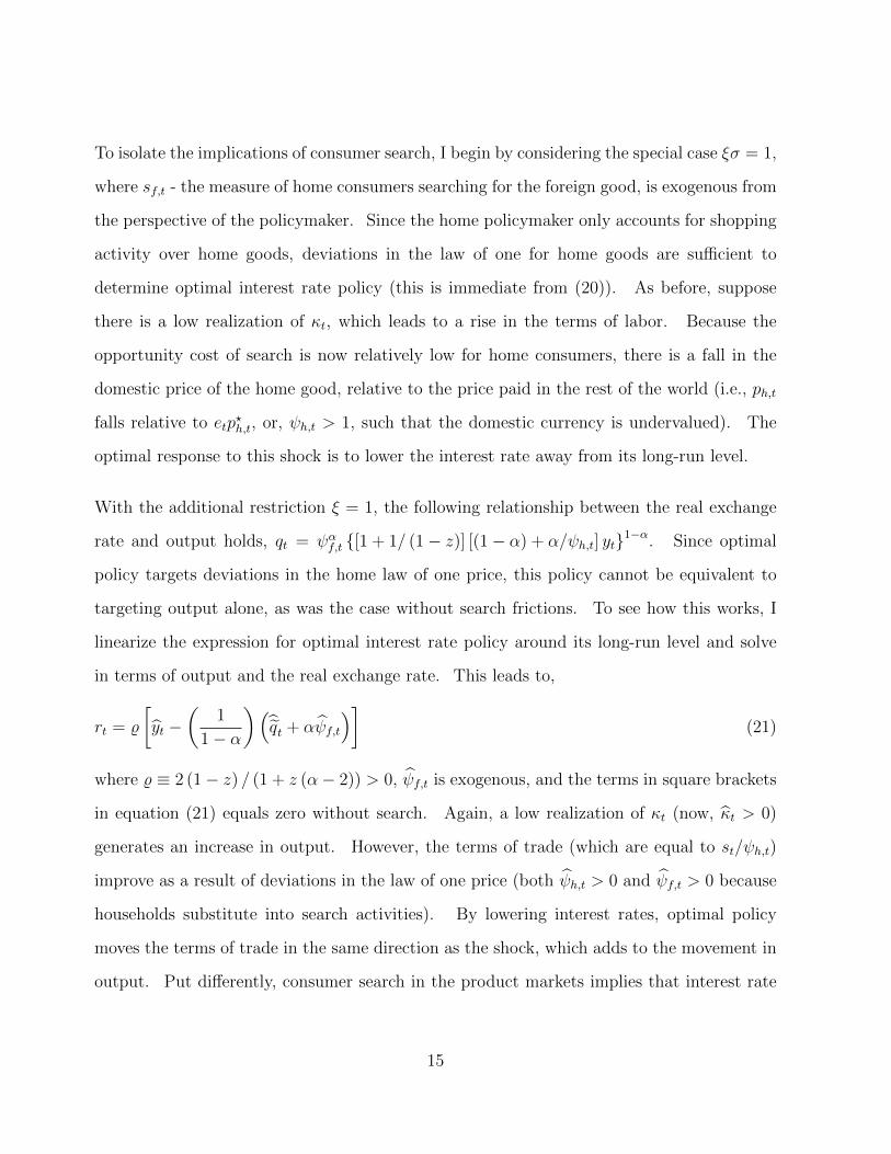
To isolate the implications of consumer search, I begin by considering the special case ξσ = 1,

where sf,t - the measure of home consumers searching for the foreign good, is exogenous from

the perspective of the policymaker. Since the home policymaker only accounts for shopping

activity over home goods, deviations in the law of one for home goods are sufficient to

determine optimal interest rate policy (this is immediate from (20)). As before, suppose

there is a low realization of κt, which leads to a rise in the terms of labor. Because the

opportunity cost of search is now relatively low for home consumers, there is a fall in the

domestic price of the home good, relative to the price paid in the rest of the world (i.e., ph,t

falls relative to etp?h,t, or, ψh,t > 1, such that the domestic currency is undervalued). The

optimal response to this shock is to lower the interest rate away from its long-run level.

With the additional restriction ξ = 1, the following relationship between the real exchange

rate and output holds, qt = ψαf,t [1 + 1/ (1− z)] [(1− α) + α/ψh,t] yt1−α. Since optimal

policy targets deviations in the home law of one price, this policy cannot be equivalent to

targeting output alone, as was the case without search frictions. To see how this works, I

linearize the expression for optimal interest rate policy around its long-run level and solve

in terms of output and the real exchange rate. This leads to,

rt = %

[yt −

(1

1− α

)(qt + αψf,t

)](21)

where % ≡ 2 (1− z) / (1 + z (α− 2)) > 0, ψf,t is exogenous, and the terms in square brackets

in equation (21) equals zero without search. Again, a low realization of κt (now, κt > 0)

generates an increase in output. However, the terms of trade (which are equal to st/ψh,t)

improve as a result of deviations in the law of one price (both ψh,t > 0 and ψf,t > 0 because

households substitute into search activities). By lowering interest rates, optimal policy

moves the terms of trade in the same direction as the shock, which adds to the movement in

output. Put differently, consumer search in the product markets implies that interest rate

15

policy is procyclical.18

3.4. The Role of Search in Generating Output Movements

In general, I want to determine how much optimal policy adds to output movements when

there is consumer search. For the sake of simplicity, consider a 1% drop in the the marginal

disutility of labor.19 Then consider variations in the trade elasticity, ξ > 0. In all cases

reported below, I fix σ (the intertemporal elasticity of substitution in consumption) at unity,

as it is only the value of this parameter, relative to the trade elasticity, that affects interest

rate policy. I also set α = 0.1, which is a measure of home-bias in consumption. In the

model with consumer search, I set z to generate a 10% markup over average prices.

Table 1 presents the change in output from the shock under optimal policy (“Optimal”) - as

characterized by equations (17) and (20) - and an interest rate peg at R = 1 (“Peg”), which

corresponds to the Friedman rule.

===== Table 1 Here =====

As we might expect, output is less volatile with search because, whilst a negative shock to the

marginal utility of labor raises output, it also generates a fall in ψh,t, which has a subsequent

negative impact on output, via the terms of trade. Moreover, under both policies (Optimal

and Peg), output is more sensitive to the shock as the trade elasticity rises, consistent with

the analytical results presented above. In the case of Walrasian product markets, since

ξ ≥ 1, policy is countercyclical as it acts to reduce movements in output, and it is more

18In fact, in this very simple case, we can write output (in levels) as, yt = (1− α)(

1κt

1Rt+

11−z

)+

α(

1κtRt+

11−z

)which is falling in κt (as is ψh,t). Since a low realization of κt requires lower interest rates

(since otherwise ψh,t would be too high) this clearly acts to stimulate output.19The details of the analysis are presented in Appendix A.3.

16

aggressive as the trade elasticity rises. When there is consumer search, policy is procyclical,

even when the trade elasticity is relatively high.

Despite the relative simplicity of the analysis, the overriding point is that the presence of

pricing-to-market and deviations from the law of one price have significant effects on policy

decisions. The model I develop is one of flexible prices but the results are analogous to

those derived within models where nominal price rigidities are present, such as Monacelli

(2005) and Engel (2011). One important difference is that I focus on the design of optimal

monetary policy following the Ramsey approach which allows for an explicit consideration of

all wedges that characterize both the long run and the short-run dynamics of the economy.

5. Conclusions

This paper derives optimal interest rate policy in a small open economy model with consumer

search frictions. In response to shocks that generate deviations from the law of one price,

optimal policy dictates that the policy stance should tighten (higher interest rates) when the

home currency is overvalued. Because policy acts in a direct way to influence deviations

from the law of one price this can lead to greater fluctuations in output.

17

Appendix

A.1 Solving for the Reservation Price

Solving the model involves finding the reservation price. Here I supply details on the deriva-

tion of equations contained in (11) as reported in the main text. Consider a good with price

pt. For such a good, the optimal condition for search implies, Wt/R′t = [pt − P (pt)] J(pt),

where pt is the reservation price and P (pt) is the expected (transacted) price. Since∫ pt0dpt = pt,

∫ pt0dJ(pt) = J(pt), and P (pt) J(pt) =

∫ pt0ptdJ(pt), we can use

∫ pt0ptdJ(pt) =

[pt × J(pt)]−∫ pt0J(pt)dpt to re-write the right-hand side of the optimal search condition as,∫ pt

0J(pt)dpt. Now we can use the distribution of the lowest price drawn by a shopper and

the distribution over price quotes, given by (3) and (10), respectively. The latter can be

expressed as, F (pt) = 1− (pt − pt) /ς (pt −Wt), where ς ≡ q/2 (1− q), and this implies,

Wt

R′t=(

1 +ςq

2

)∫ pt

pt

dpt −ςq × (pt −Wt)

2

2

∫ pt

pt

(1

pt −Wt

)2

dpt (22)

where pt

is determined by F(pt

)= 0, and since, in equilibrium, the highest price is equal to

the shoppers reservation price, pt = pt (Burdett and Judd, 1983). Using∫

[1/ (pt −Wt)]2 dpt =

−1/ (pt −Wt) and∫dpt = pt and the condition for the lower support of the distribu-

tion, F(pt

)= 0, I generate the following reservation price, pt = Wt + [1/ (1− q)]Wt/R

′t.

In the text, I also report the transacted price, P (pt). The reservation and transacted

price have a very simple relationship. To see why, note, P (pt) =∫ ppt

ptfT (pt) dpt, where

fT (pt) ≡ f (pt) d (pt) is the transacted price density, and d (pt) = q + 2 (1− q) [1− F (pt)] is

the demand curve per-shopper.

A.2. Monetary Policy Problem with Product Search

In the home economy, the monetary authority maximizes∑∞

t=0 βt [lnu (ct)− κ (lt + st)]. Us-

ing the definitions, ρt = pf,t/ph,t and ρ?t = p?f,t/p?h,t, resources conditions can be written as,

lt = (1− α) [g (ρt)]ξ ct + α (ρ?t )

ξ c?t ; st =[(1− α) ct + αρ−ξt

][g (ρt)]

ξ ct (23)

18

In both constraints I eliminate home consumption for foreign consumption (which is ex-

ogenous) using the risk-sharing condition. The final step involves eliminating the variable

ρ?t = ρt (ψf,t/ψh,t). From the perspective of the home policy maker ψf,t is exogenous as it

is only a function of the shock and the rest of world nominal interest rate, which is set at

unity. Note that the variable ρt and the law of one price gap are not independent choice

variables. In particular, I write ψh,t = 1 + φtρt, where φt ≡ (1− κt) / [(1− z) + κt]. Using

this relation, I re-express the output-resource constraint as,

lt = (1− α) [g (ρt)]ξ ct + α

(ρt

1 + φtρtψf,t

)ξc?t (24)

Finally, to derive the expression presented in the text, note g′ (·) = α [g (ρt) /ρt]ξ and q′ (·) =

ψf,t (1− α) [g (ρt)]ξ−2.

A.3. Derivations for Calculation of Output Movements

I first linearize the resource equations around R > 1. For output,

yt = (ξ − 1) gt +(ξ − 1)α

α + (1− α) q1−ξqt − ξα

α + (1− α) q1−ξψh,t −

(R

R + 11−z

)Rt − κt (25)

and shopping,

st = (ξ − 1) gt −ξα

α + (1− α) ρξρt −

(R

R + 11−z

)Rt − κt (26)

which is only relevant for policy decisions when ξ 6= 1. International relative prices are linked

by, gt = α (ρ/g)1−ξ ρt and qt = ψf,t + (1− α) (ρ/q)ξ−1 ρt. When R = 1, then ρ = g = q = 1,

and we can solve for the the output response to the shock easily as,

yt = (ξ − 1)α[(2− α) ρt + ψf,t

]− ξαψh,t − κt (27)

where ρt = −κt/(1 + 1

1−z

)and ψh,t = ψf,t =

(1

1−z

)ρt. I determine R > 1 under optimal

policy by solving (25), (26) and (20) jointly as a non-linear system. To determine the

response of output to the shock, I linearize (20) around its long-run level.

19

References

ALESSANDRIA, G. (2009), “Consumer Search, Price Dispersion, and International Relative

Price Fluctuations”, International Economic Review 50, 803-829.

ALESSANDRIA, G. and KABOWSKI, J. (2011), “Pricing to Market and the Failure of

Absolute PPP”, American Economic Journal: Macroeconomics 3, 91-127.

ARSENEAU, D., CHAHROUR, R., CHUGH, S. and SHAPIRO, A. (2014), “Optimal Fis-

cal and Monetary Policy in Customer Markets”, Journal of Money, Credit, and Banking,

forthcoming.

ATKESON, A. and BURSTEIN, A. (2008), “Pricing-to-Market, Trade Costs, and Interna-

tional Relative Prices”, American Economic Review 98, 1998-2031.

BAI, Y. and RIOS-RULL, V. (2013), “Demand Shocks and Open Economy Puzzles”, mimeo,

Rochester.

BACKUS, D. K., KEHOE, P. J. and KYDLAND, F. E. (1995), “International Business

Cycles: Theory and Evidence”, in T. F. Cooley (ed.), Frontiers of Business Cycle Research

(Princeton: Princeton University Press) 331-356.

BANERJEE, A. and RUSSELL, B. (2001), “The Relationship Between the Markup and

Inflation in the G7 Economies and Australia”, Review of Economics and Statistics 83, 377-

384.

BENABOU, R. (1992), “Inflation and Markups: Theories and Evidence from the Retail

Trade Sector”, European Economic Review 36, 566-574.

BENIGNO, G. and BENIGNO, P. (2003), “Price Stability in Open Economies”, Review of

Economic Studies 70, 743-764.

BURDETT, K. and JUDD, K. (1983), “Equilibrium Price Dispersion”, Econometrica 51,

955-969.

20

CHARI, V., KEHOE, P., and MCGRATTEN, E. (2002), “Can Sticky Price Models Generate

Volatile and Persistent Real Exchange Rates?”, Review of Economic Studies 69, 533-563.

CHARI, V., KEHOE, P., and MCGRATTEN, E. (2007), “Business Cycle Accounting”,Econometrica

75, 781-836.

CORNIA, M., GERARDI, K. and HALE SHAPIRO, A. (2012), “Price Dispersion Over the

Business Cycle: Evidence from the Airline Industry”, Journal of Industrial Economics 60,

347-373.

CORSETTI, G., DEDOLA, L. and LEDUC, S. (2008), “International Risk-Sharing and the

Transmission of Productivity Shocks”, Review of Economic Studies 75, 443-473.

CORSETTI, G., DEDOLA, L. and LEDUC, S. (2010), “Optimal Monetary Policy and the

Sources of Local-Currency Price Stability” In International Dimensions of Monetary Policy,

ed. Jordi Galı and Mark Gertler, 319-367. Chicago: University of Chicago Press.

DROZD, L. and NOSAL, J. (2012), “Understanding International Prices: Customers as

Capita”, American Economic Review 102, 364-395.

DROZD, L. and NOSAL, J. (2013), “Pricing-to-Market in Business Cycle Models”, mimeo,

Wharton.

ENGEL, C. (2011), “Currency Misalignments and Optimal Monetary Policy: A Reexami-

nation”, American Economic Review 101, 2796-2822.

FAIA, E. and MONACELLI, T. (2008), “Optimal Monetary Policy in a Small Open Economy

with Home Bias”, Journal of Money, Credit, and Banking 40, 721-750.

HALL, R. (1997), “Macroeconomic Fluctuations and the Allocation of Time”, Journal of

Labor Economics 15, 223-250.

HEATHCOTE, J. and PERRI, F. (2002), “Financial Autarky and International Business

Cycles”, Journal of Monetary Economics, 49, 601-627.

21

HEAD, A., LIU, L., MENZIO, G. and WRIGHT, R. (2012), “Sticky Prices: A New Mone-

tarist Approach”, Journal of the European Economic Association 10, 1-36.

HOLLAND, A. and SCOTT, A. (1998), “The Determinants of UK Business Cycles”, Eco-

nomic Journal 108, 1067-1092.

ITSKHOKI, O. and GOPINATH, G. (2010), “Currency Choice and Exchange Rate Pass-

through”, American Economic Review 83, 473-486.

KAPLAN, G. and MENZIO, G. (2013), “Shopping Externalities and Self-Fulfilling Unem-

ployment Fluctuations”, mimeo, Princeton.

KARABARBOUNIS, L. (2014), “Home Production, Labor Wedges, and International Busi-

ness Cycles”, Journal of Monetary Economics 64, 68-84.

LUCAS, R. and STOKEY, N. (1983), “Optimal Fiscal and Monetary Theory in an Economy

without Capital”, Journal of Monetary Economics 12, 55–93.

LUI, Q. and SHI, S. (2010), “Currency Areas and Monetary Coordination”, International

Economic Review 51, 813–836.

MONACELLI, T. (2005), “Monetary Policy in a Low Pass-through Environment”, Journal

of Money, Credit and Banking 37, 1047-1066.

NAKAJIMA, T. (2005), “A Business Cycle Model with Variable Capacity Utilization and

Demand Disturbances”, European Economic Review 49, 1331-1360.

NEKARDA, C. and RAMEY, V. (2013), “The Cyclical Behavior of the Price-Cost Markup”,

mimeo, UCSD.

SHI, S. and LIU, Q. (2010), “Currency Areas and Monetary Coordination”, International

Economic Review 51, 813-836.

22

Table 1: Output Movements and Interest Rate Policies

Trade Elasticity: ξ

1 1.2 1.8

Product Market Peg Optimal Peg Optimal Peg Optimal

Walrasian 1 1 1.04 1.02 1.15 1.11

Consumer Search 0.95 1 0.96 1.01 1.01 1.08

23