Principles of Operating Systems

Lecture 9-10 - CPU SchedulingArdalan Amiri Sani (ardalan@uci.edu)

[lecture slides contains some content adapted from previous slides by Prof. Nalini Venkatasubramanian, and course text slides © Silberschatz]

2

Outline● Basic Concepts● Scheduling Objectives● Levels of Scheduling● Scheduling Criteria● Scheduling Algorithms

● FCFS, Shortest Job First, Priority, Round Robin, Multilevel

● Multiple Processor Scheduling● Real-time Scheduling● Algorithm Evaluation

3

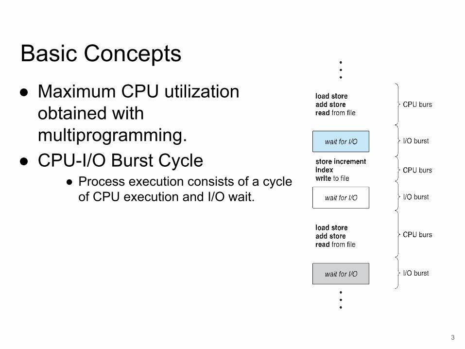
Basic Concepts● Maximum CPU utilization

obtained with multiprogramming.

● CPU-I/O Burst Cycle● Process execution consists of a cycle

of CPU execution and I/O wait.

4

CPU Burst Distribution

5

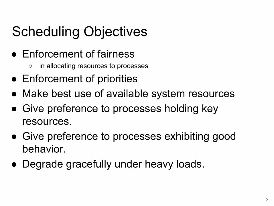
Scheduling Objectives● Enforcement of fairness

○ in allocating resources to processes

● Enforcement of priorities● Make best use of available system resources● Give preference to processes holding key

resources.● Give preference to processes exhibiting good

behavior.● Degrade gracefully under heavy loads.

6

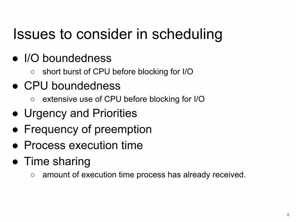
Issues to consider in scheduling● I/O boundedness

○ short burst of CPU before blocking for I/O

● CPU boundedness○ extensive use of CPU before blocking for I/O

● Urgency and Priorities● Frequency of preemption● Process execution time● Time sharing

○ amount of execution time process has already received.

7

Levels of Scheduling● High Level Scheduling or Job Scheduling

○ Selects jobs allowed to compete for CPU and other system resources.

● Low Level (CPU) Scheduling or Dispatching○ Selects the ready process that will be assigned the CPU.○ Ready Queue contains PCBs of processes ready to be

dispatched.

● Intermediate Level Scheduling or Medium Term Scheduling

○ Selects which jobs to temporarily suspend/resume to smooth fluctuations in system load.

8

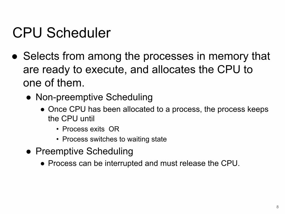
CPU Scheduler● Selects from among the processes in memory that

are ready to execute, and allocates the CPU to one of them.● Non-preemptive Scheduling

● Once CPU has been allocated to a process, the process keeps the CPU until

• Process exits OR• Process switches to waiting state

● Preemptive Scheduling● Process can be interrupted and must release the CPU.

• Need to coordinate access to shared data

9

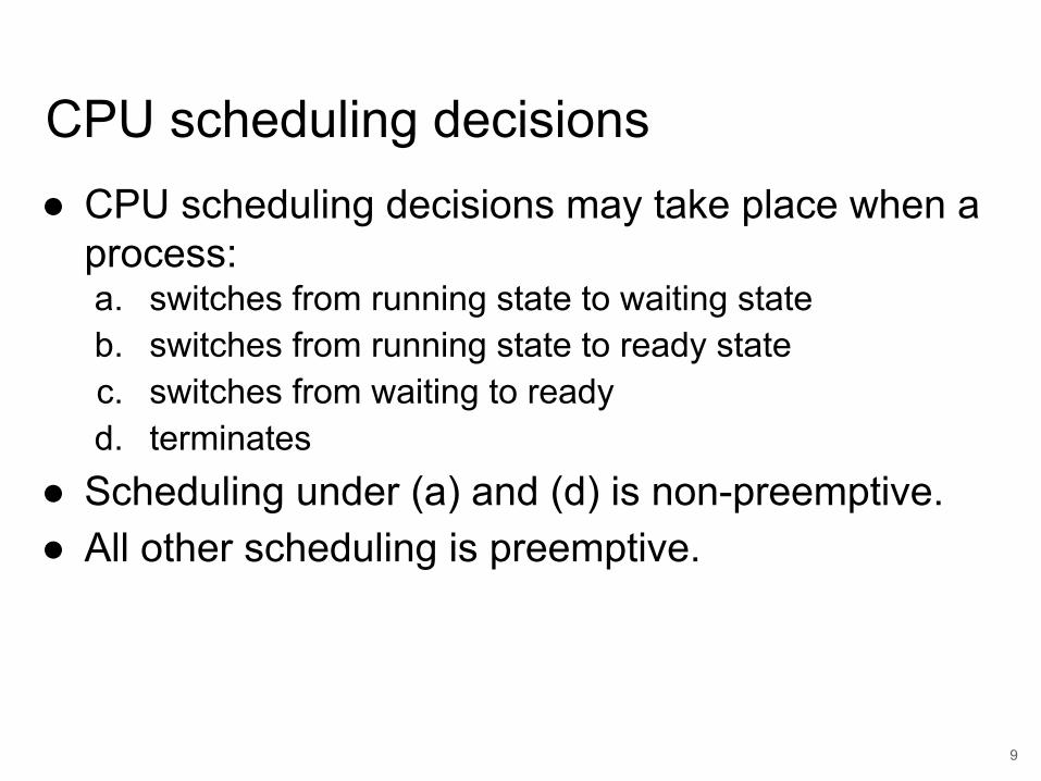
CPU scheduling decisions● CPU scheduling decisions may take place when a

process:a. switches from running state to waiting stateb. switches from running state to ready statec. switches from waiting to readyd. terminates

● Scheduling under (a) and (d) is non-preemptive.● All other scheduling is preemptive.

10

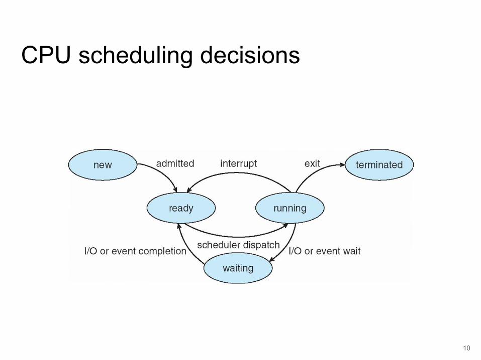
CPU scheduling decisions

new admitted

interrupt

I/O oreventcompletion

Schedulerdispatch I/O or

event wait

exit terminated

waiting

ready running

11

Dispatcher● Dispatcher module gives control of the CPU to the

process selected by the short-term scheduler. This involves:

• switching context• switching to user mode• jumping to the proper location in the user program to restart that

program

● Dispatch Latency:● time it takes for the dispatcher to stop one process and start

another running.● Dispatcher must be fast.

12

Scheduling Criteria● CPU Utilization

● Keep the CPU and other resources as busy as possible

● Throughput ● # of processes that complete their execution per time unit.

● Turnaround time ● amount of time to execute a particular process from its entry

time.

13

Scheduling Criteria (cont.)● Waiting time

● amount of time a process has been waiting in the ready queue.

● Response Time (in a time-sharing environment)● amount of time it takes from when a request was submitted until

the first response (and NOT the final output) is produced.

14

Optimization Criteria● Max CPU Utilization● Max Throughput● Min Turnaround time● Min Waiting time● Min response time

15

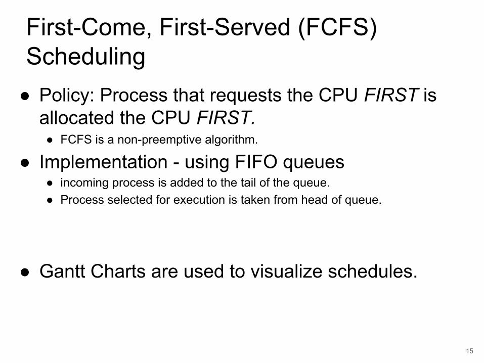
● Policy: Process that requests the CPU FIRST is allocated the CPU FIRST.

● FCFS is a non-preemptive algorithm.

● Implementation - using FIFO queues● incoming process is added to the tail of the queue.● Process selected for execution is taken from head of queue.

● Performance metric - Average waiting time in queue.

● Gantt Charts are used to visualize schedules.

First-Come, First-Served (FCFS) Scheduling

First-Come, First-Served (FCFS) Scheduling

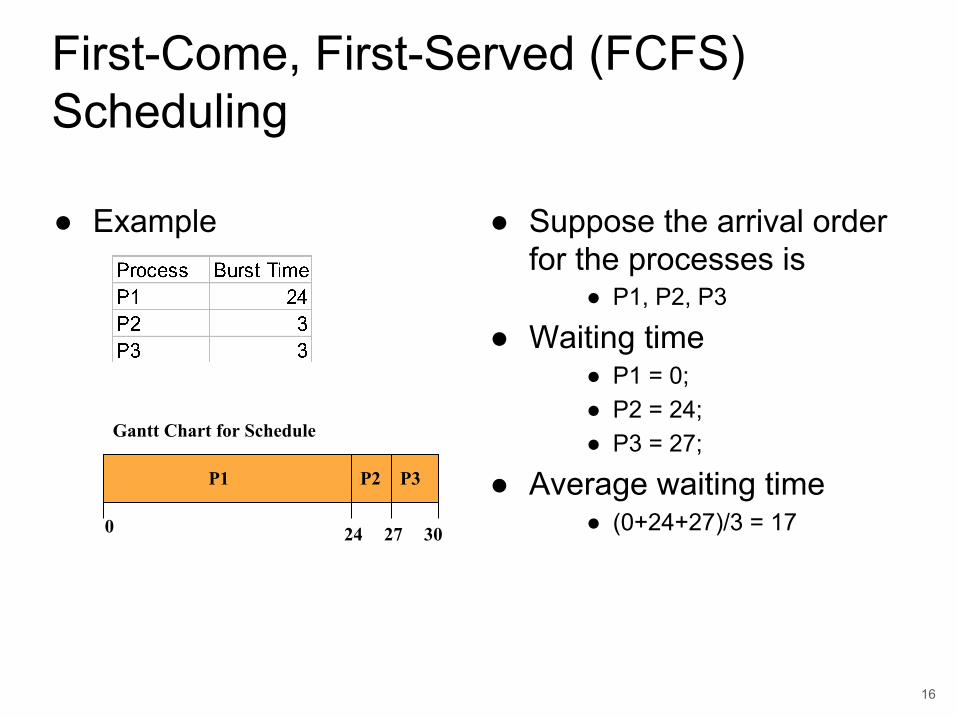
● Example ● Suppose the arrival order for the processes is

● P1, P2, P3

● Waiting time ● P1 = 0;● P2 = 24;● P3 = 27;

● Average waiting time● (0+24+27)/3 = 170 24 27 30

P1 P2 P3

Gantt Chart for Schedule

16

FCFS Scheduling (cont.)

● Example ● Suppose the arrival order for the processes is

● P2, P3, P1

● Waiting time ● P1 = 6; P2 = 0; P3 = 3;

● Average waiting time● (6+0+3)/3 = 3 , better..

● Convoy Effect:● short processes waiting

behind long process, e.g., 1 CPU bound process, many I/O bound processes.

0 3 6 30

P1P2 P3

Gantt Chart for Schedule

17

18

Shortest-Job-First (SJF) Scheduling● Associate with each process the length of its next CPU

burst. Use these lengths to schedule the process with the shortest time.

● Two Schemes:● Scheme 1: Non-preemptive

• Once CPU is given to the process it cannot be preempted until it completes its CPU burst.

● Scheme 2: Preemptive• If a new CPU process arrives with CPU burst length less than

remaining time of current executing process, preempt. Also called Shortest-Remaining-Time-First (SRTF).

● SJF is optimal - gives minimum average waiting time for a given set of processes.• The difficulty is knowing the length of the next CPU request• Could ask the user

19

Non-Preemptive SJF Scheduling● Example

0 8 16

P1 P2P3

Gantt Chart for Schedule

P4

127

Average waiting time = (0+6+3+7)/4 = 4

20

Non-Preemptive SJF Scheduling Process Arrival Time Burst Time

P1 0.0 0 6

P2 2.0 2 8

P3 4.0 5 7

P4 5.0 0 3

● SJF scheduling chart

● Average waiting time = ((3-0) + (16-2) + (9-5) + 0) / 4 = 5.25

● Average turnaround time = ((9-0) + (24-2) + (16-5) + (3-0))/4 = 11.25

46

21

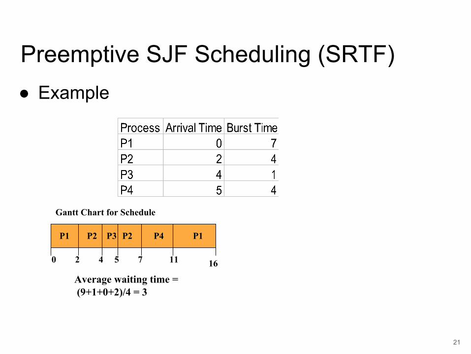
Preemptive SJF Scheduling (SRTF)● Example

0 7 16

P1 P2P3

Gantt Chart for Schedule

P4

115

Average waiting time = (9+1+0+2)/4 = 3

P2 P1

2 4

22

Preemptive SJF Scheduling (SRTF)● Now we add the concepts of varying arrival times and preemption to the analysis

ProcessA arri Arrival Time Burst Time

P1 0 8

P2 1 4

P3 2 9

P4 3 5

● Preemptive SJF Gantt Chart

● Average waiting time = [(10-1)+(1-1)+(17-2)+5-3)]/4 = 26/4 = 6.5 msec

● Average turnaround time = ((17-0) + (5-1) + (26-2) + (10-3))/4 = 13 msec

0 7 6

23

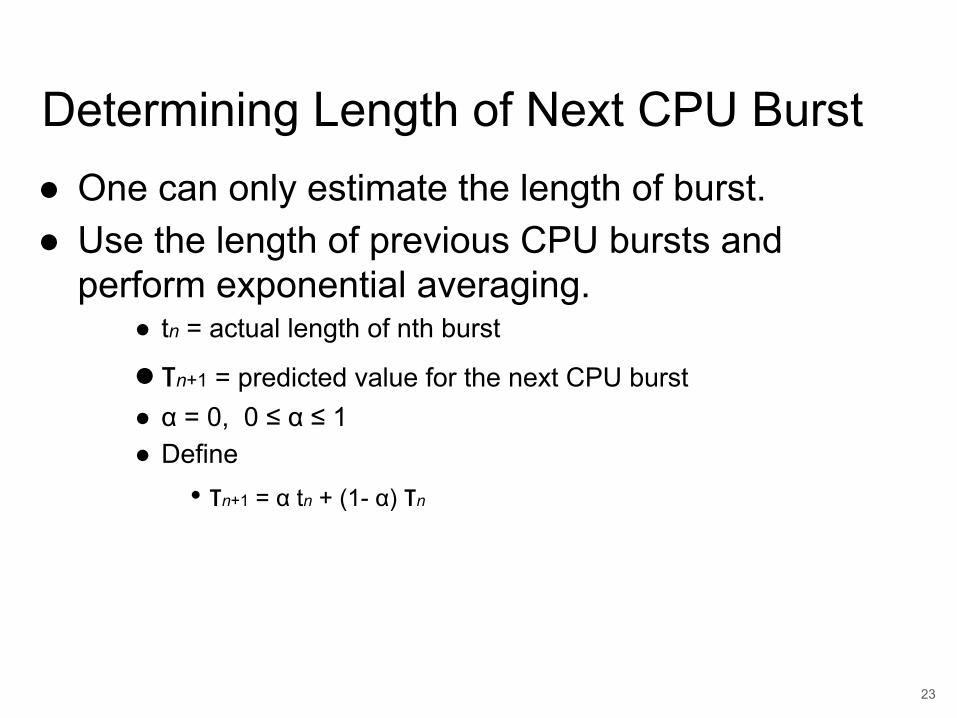
Determining Length of Next CPU Burst● One can only estimate the length of burst.● Use the length of previous CPU bursts and

perform exponential averaging.● tn = actual length of nth burst

● τn+1 = predicted value for the next CPU burst● α = 0, 0 ≤ α ≤ 1● Define

• τn+1 = α tn + (1- α) τn

24

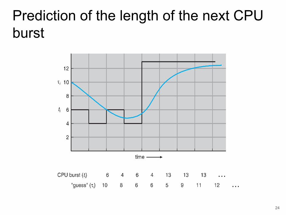
Prediction of the length of the next CPU burst

25

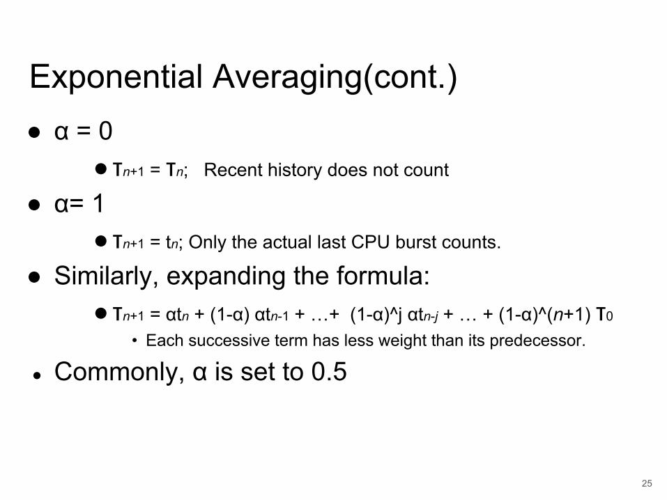
Exponential Averaging(cont.)● α = 0

● τn+1 = τn; Recent history does not count

● α= 1● τn+1 = tn; Only the actual last CPU burst counts.

● Similarly, expanding the formula:● τn+1 = αtn + (1-α) αtn-1 + …+ (1-α)^j αtn-j + … + (1-α)^(n+1) τ0

• Each successive term has less weight than its predecessor.

● Commonly, α is set to 0.5

j

26

Priority Scheduling● A priority value (integer) is associated with each

process. Can be based on○ Cost to user○ Importance to user○ Aging○ %CPU time used in last X hours.

● CPU is allocated to the process with the highest priority.

○ Preemptive○ Nonpreemptive

27

Priority Scheduling (cont.)● SJF is a priority scheme where the priority is the

predicted next CPU burst time.● Problem

● Starvation!! - Low priority processes may never execute.

● Solution● Aging - as time progresses increase the priority of the process.

28

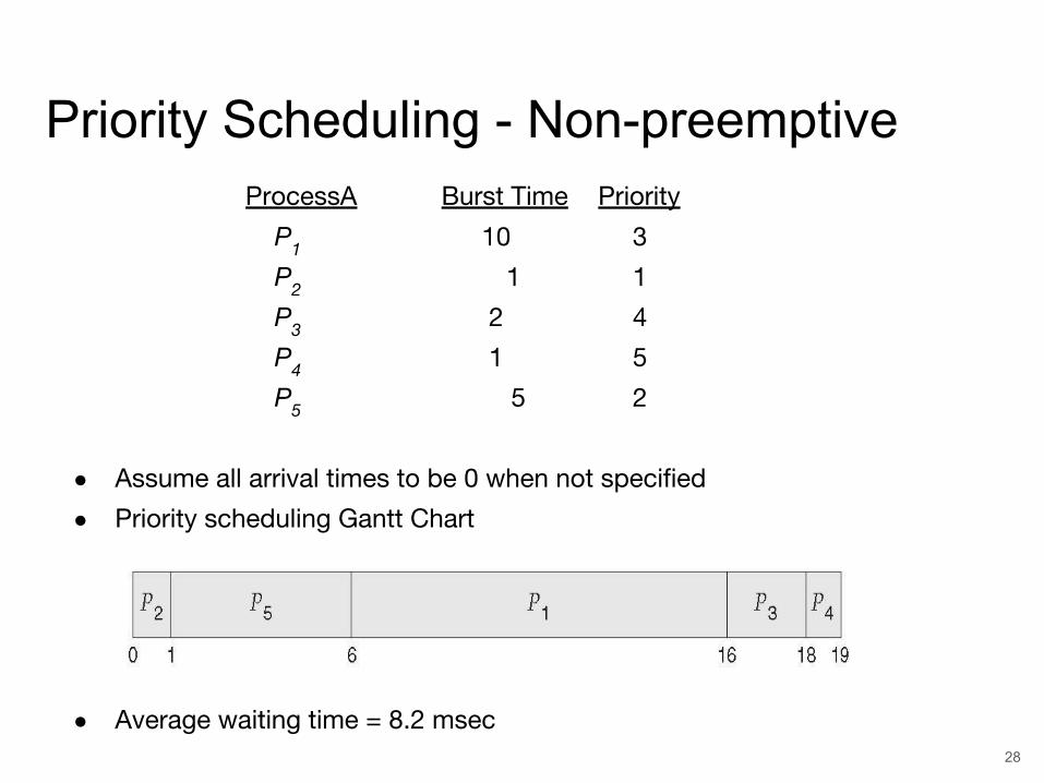
Priority Scheduling - Non-preemptive ProcessA Burst Time Priority

P1 10 3

P2 1 1

P3 2 4

P4 1 5

P5 5 2

● Assume all arrival times to be 0 when not specified

● Priority scheduling Gantt Chart

● Average waiting time = 8.2 msec

29

Priority Scheduling - Preemptive ProcessA Burst Time Priority Arrival Time

P1 6 3 12

P2 8 2 0

P3 7 4 4

P4 3 1 2

P5 5 5 30

● Gantt Chart

● Average waiting time = [0+3+(7+6)+0+0)]/5 = 16/5 = 3.2 msec

● Average turnaround time = (6 + 11 + 20 + 3 + 5)/5 = 45/5 = 9 msec

● Average response time (assuming immediate response by a process when executed) = (0 + 0 + 7 + 0 + 0) / 5 = 1.4 msec

● CPU utilization = 29 / 35 = 0.83 = 83%

● Throughput = 5 / 35 = 0.14 #process/msec

0

P2

2 5 11 12 18 24 30 35

P4 P2 P3 P1 P3 P5

30

Round Robin (RR)● Each process gets a small unit of CPU time

• Time quantum usually 10-100 milliseconds. • After this time has elapsed, the process is preempted and added

to the end of the ready queue.● n processes, time quantum = q

• Each process gets 1/n CPU time in chunks of at most q time units at a time.

• No process waits more than (n-1)q time units.• Performance

– Time slice q too large - FIFO behavior– Time slice q too small - Overhead of context switch is too expensive.– Heuristic - 70-80% of jobs block within timeslice

31

Round Robin Example● Time Quantum = 20

0

P1 P4P3

Gantt Chart for Schedule

P1P2

20

P3 P3 P3P4 P1

37 57 77 97 117 121 134 154 162

Typically, higher average turnaround time than SRTF, but better response

32

Round Robin ExampleProcess Burst TimeP1 24 P2 3 P3 3

● The Gantt chart is (quantum = 4):

● Average waiting time = (6 + 4 + 7)/3 = 5.67● Average turnaround time = (30 + 7 + 10)/3 = 11.75

0 4 7 10 14 18 22 26 30

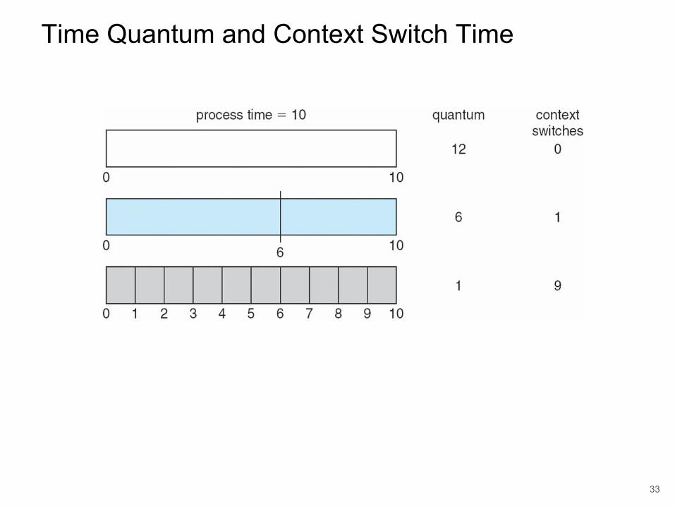
Time Quantum and Context Switch Time

33

Turnaround Time Varies With The Time Quantum

80% of CPU bursts should be shorter than q

34

35

Multilevel Queue● Ready Queue partitioned into separate queues

○ Example: system processes, foreground (interactive), background (batch), student processes….

● Each queue has its own scheduling algorithm○ Example: foreground (RR), background (FCFS)

● Processes assigned to one queue permanently.● Scheduling must be done between the queues

○ Fixed priority - serve all from foreground, then from background. Possibility of starvation.

○ Time slice - Each queue gets some CPU time that it schedules - e.g. 80% foreground (RR), 20% background (FCFS)

36

Multilevel Queue scheduling

37

Multilevel Feedback Queue

● A process can move between the queues.○ Aging can be implemented this way.

● Parameters for a multilevel feedback queue scheduler:

○ number of queues.○ scheduling algorithm for each queue and between queues.○ method used to determine when to upgrade a process.○ method used to determine when to demote a process.○ method used to determine which queue a process will enter when that

process needs service.

38

Multilevel Feedback Queue● Example: Three Queues -

○ Q0 - RR with time quantum 8 milliseconds○ Q1 - RR with time quantum 16 milliseconds○ Q2 - FCFS

● Scheduling○ New job enters Q0 - When it gains CPU, it

receives 8 milliseconds. If job does not finish, move it to Q1.

○ At Q1, when job gains CPU, it receives 16 more milliseconds. If job does not complete, it is preempted and moved to queue Q2.

Thread Scheduling

● When threads supported, threads scheduled, not processes

● In many-to-one and many-to-many models, thread library schedules user-level threads to run on a kernel thread.LWP● Known as process-contention scope (PCS) since scheduling

competition is within the process● Typically done via priority set by programmer

● The CPU scheduler schedules the kernel threads.Kernel thread scheduled onto available CPU is system-contention scope (SCS) – competition among all threads in system

39

40

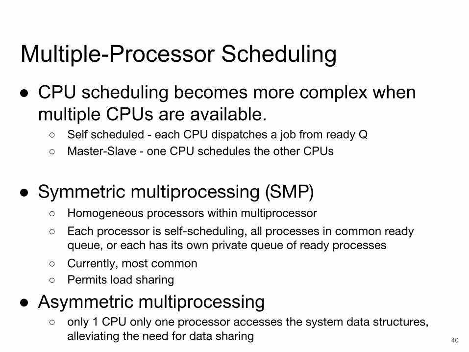
Multiple-Processor Scheduling● CPU scheduling becomes more complex when

multiple CPUs are available.○ Self scheduled - each CPU dispatches a job from ready Q○ Master-Slave - one CPU schedules the other CPUs○ Have one ready queue accessed by each CPU.

● Symmetric multiprocessing (SMP)○ Homogeneous processors within multiprocessor○ Each processor is self-scheduling, all processes in common ready

queue, or each has its own private queue of ready processes

○ Currently, most common○ Permits load sharing

● Asymmetric multiprocessing ○ only 1 CPU only one processor accesses the system data structures,

alleviating the need for data sharing

NUMA and CPU Scheduling: considers processor affinity

Note that memory-placement algorithms can also consider affinity

41

NUMA and CPU Scheduling: considers processor affinity

42Image source: https://www.supermicro.com/products/motherboard/Xeon/C620/X11DPi-N.cfm

Supermicro X11DPi-N motherboard

Multicore Processors

● Recent trend to place multiple processor cores on same physical chip

● Faster and consumes less power

43

Hyperthreading

● Multiple threads per core● Takes advantage of memory stall to make progress on

another thread while memory retrieve happens● One CPU core looks like two cores to the operating system

with hyperthreading

44

Hyperthreading

45

46

Algorithm Evaluation● Deterministic Modeling

○ Takes a particular predetermined workload and defines the performance of each algorithm for that workload. Too specific, requires exact knowledge to be useful.

● Queuing Models and Queuing Theory○ Use distributions of CPU and I/O bursts. Knowing arrival and service

rates - can compute utilization, average queue length, average wait time etc…

○ Little’s formula - n = λ×W where n is the average queue length, λ is the avg. arrival rate and W is the avg. waiting time in queue.

● Other techniques: Simulations, Implementation