privatization and changes in the wage structure: evidence from
TRANSCRIPT

IZA DP No. 3760
Privatization and Changes in the Wage Structure:Evidence from Firm Personnel Records
Blaise MellyPatrick A. Puhani
DI
SC
US
SI
ON
PA
PE
R S
ER
IE
S
Forschungsinstitutzur Zukunft der ArbeitInstitute for the Studyof Labor
October 2008

Privatization and Changes in the Wage
Structure: Evidence from Firm Personnel Records
Blaise Melly Brown University
Patrick A. Puhani
Leibniz Universität Hannover, SIAW, University of St. Gallen,
ERMES, Université Paris II and IZA
Discussion Paper No. 3760 October 2008
IZA
P.O. Box 7240 53072 Bonn
Germany
Phone: +49-228-3894-0 Fax: +49-228-3894-180
E-mail: [email protected]
Any opinions expressed here are those of the author(s) and not those of IZA. Research published in this series may include views on policy, but the institute itself takes no institutional policy positions. The Institute for the Study of Labor (IZA) in Bonn is a local and virtual international research center and a place of communication between science, politics and business. IZA is an independent nonprofit organization supported by Deutsche Post World Net. The center is associated with the University of Bonn and offers a stimulating research environment through its international network, workshops and conferences, data service, project support, research visits and doctoral program. IZA engages in (i) original and internationally competitive research in all fields of labor economics, (ii) development of policy concepts, and (iii) dissemination of research results and concepts to the interested public. IZA Discussion Papers often represent preliminary work and are circulated to encourage discussion. Citation of such a paper should account for its provisional character. A revised version may be available directly from the author.

IZA Discussion Paper No. 3760 October 2008
ABSTRACT
Privatization and Changes in the Wage Structure: Evidence from Firm Personnel Records*
We investigate the wage effects of privatization using person-level firm-based panel datasets from one privatized and one nonprivatized public sector firm in the same country for the years immediately before and after privatization. Thus, we can analyze the before-after effects of privatization while controlling for individual and time fixed effects and allowing for firm-specific trends. Because the change in wage regime coincides with substantial losses in the market share of the privatized but not the nonprivatized firm, the situation approximates a natural experiment in switching workers from the public to the private sector. We find significant changes in the wage structure of the privatized but not the nonprivatized firm. Specifically, wage and wage growth distributions widened significantly after privatization. Conditioning on worker characteristics, we find that younger employees and those with shorter tenure gained from privatization, while high-skilled workers gained relative to medium-skilled workers. Surprisingly, low-skilled workers also gained, although seemingly in the form of temporary compensation intended to increase acceptance of privatization. JEL Classification: J31, J45, L33 Keywords: privatization, liberalization, competition, labor markets, wage distributions Corresponding author: Patrick A. Puhani Leibniz Universität Hannover Institut für Arbeitsökonomik Königsworther Platz 1 D-30167 Hannover Germany E-mail: [email protected]
* Part of this project was supported by the German Research Foundation (Deutsche Forschungsgemeinschaft) under the project Labour Market Effects of Social Policy (Arbeitsmarkteffekte sozialpolitischer Maßnahmen). In its initial phase, the project was supported by the Swiss National Science Foundation NFP 4045. We thank several employees (not mentioned here by name) for help with institutional and data questions relating to their respective companies. The railway company requested the inclusion of the following disclaimer: “The railway company welcomes the interest in its company and supports research by providing its data. The current study does, however, not necessarily reflect the opinion of the railway company. The railway company therefore reserves the right to produce a contrary view.” A similar disclaimer applies to the telecommunications company. We are grateful to David Autor, Michael Lechner, Eric Maurin, Terra G. McKinnish, Michael Pollitt, Ken Troske, Josef Zweimüller, seminar participants at the Universities of St. Gallen, Hannover, ERMES-Panthéon-Assas (Paris II), Paris School of Economics, the Annual Meeting of the Labour and Population Economics Group of the German Economic Association in Basle, the meeting of the German Research Foundation Group, “Flexibility in Heterogeneous Labour Markets,” in Bonn and Mannheim, the Society of Labor Economists (SOLE) Annual Meetings in Chicago, the Annual Congresses of the European Economic Association in Budapest, and the German Economic Association in Munich for helpful comments. Michael Huber and Juliane Parys provided excellent research assistance.
1
I. Introduction
Until 1979, the state in all major European industrialized countries owned at least the
telecommunications and postal services, gas and electricity utilities, and the airlines and railway
companies. In the United States, on the other hand, state intervention in many of these sectors
took the form of regulated monopolies rather than state ownership. Since then, however, changes
in technology, as well as changes in the perception of market versus government or regulatory
failure, have generated policies of deregulation or privatization on both sides of the Atlantic. In
Europe, British Prime Minister Margaret Thatcher launched a large privatization program under
which the share of state-owned enterprises in the UK economy declined from more than 10
percent to almost zero between 1979 and 1997.1 The perceived success of this British
privatization program persuaded many other industrialized countries to sell publicly owned
companies and foster competition, which resulted, for example, in the 82 percent private
ownership of telecommunications operators in developed countries in 2003 from almost zero in
1980.2 On both sides of the Atlantic, deregulation and privatization had the aim of raising
productive efficiency by competition. For many of Europe’s industries, which – like in the case of
telecommunications analyzed in this paper – were state-owned, competition could only be
effectively introduced with some form of privatization, because “it may be difficult to introduce
rivalry without some private ownership” (Vickers and Yarrow, 1991, p. 117).
In this paper, we analyze the changes in the wage structure of a telecommunications
company before and after privatization. International agreements forced the country in question to
allow competition in its telecommunications sector, so that privatization and the introduction of
competition occurred virtually at the same time (and late rather than early in international
1 See Megginson and Netter (2001).

2
comparison). Our situation thus approximates a natural experiment where workers are taken from
a non-competitive environment like the public administration (indeed the same pay scales applied
in the firm and the administration before privatization) to a private firm operating in a
competitive market.
The impact of such privatization on the economic and financial performance of divested
firms, investment returns, the development of capital markets, and corporate government
practices has been examined quite intensively (e.g., Megginson and Netter, 2001). However
surprisingly, the effects of privatization on employment structures and particularly on wages have
been neglected. Thus, Megginson and Netter (2001) conclude their survey by pointing to aspects
of privatization that must be better understood, including the conclusive documentation of “the
labor economics of privatization programs” (p.382). Documenting the effect of privatization on
wage structure is the objective of our paper.
The public sector represents an important opportunity to analyze the labor market
behavior of a monopolist since the share of public sector employment in most industrialized
countries is still around 15–20 percent (Gregory and Borland, 1999). Despite substantial literature
documenting and comparing public and private sector wages, there is little experimental evidence
on differences between public and private sector wage structures, only descriptive empirical
findings of a public sector wage premium, especially for women and racial minorities.
Descriptive (international) observations also indicate that the public sector compresses both
unconditional and conditional wage distributions.3 The question of whether these results are
driven by worker self-selection into either of these two sectors remains open.
Therefore, empirical studies have relied on deregulation or privatization to generate
exogenous variation in market concentration. Most studies using firm- or industry-level data find
2 Based on data from the International Telecommunications Union (ITU).

3
that workers lose rents through deregulation or privatization in terms of employment and wages
(Haskel and Szymanski, 1993; Bertrand and Mullainathan, 2003; Azmat, Manning, and Van
Rennen, 2007), although this may not be true for all occupational groups (see Card, 1986;
Johnson, 1991; Batt, 2001, on the airline industry). Rose (1987), Hirsch (1988), Peoples and
Saunders (1993), Peoples (1998), Peoples and Talley (2001), Black and Strahan (2001) and
Wozniak (2007), on the other hand, use person-level data and analyze issues such as the effect of
deregulation and privatization on union, white and male workers’ rents. They all use data from
the Current Population Survey that does not have a significant panel structure and thus these
authors do not control for person-level fixed effects.4
In contrast to these studies, and this is a particular strength of our paper, we use person-
level panel data from a firm’s complete personnel records in order to trace the changes in the
wage structure before, at, and after the wage regime switch from the public to the private sector.
Our unique panel includes all employees in two firms located in the same (nontransitional)
industrialized country,5 one operating in the telecommunications sector and the second in the
railway industry. The panel structure of the data allows us to follow these firms’ employees for
five consecutive years. The telecommunications firm switches its wage regime from public to
private sector regulations for all workers two years after the start of our observation period, a
wage structure change that coincides with substantial losses in its market share. We therefore
expect the change in wage regime to be profound and the timing of the reform to be more clearly
defined than in many cases of deregulation analyzed elsewhere. On the other hand, the quasi-
simultaneity of the changes in the company’s legal status and market shares makes it impossible
3 Gregory and Borland (1999) survey this literature. 4 The Current Population Survey actually has a very short panel component (4 months in, 8 months out, 4
months in, then out for good), which has not been used by these authors. The importance of unobserved individual heterogeneity is demonstrated by Hirsch (1993) and Belman and Monaco (2001) using the short (two-year) panel component of the CPS (see also Guadalupe, 2007, for similar evidence on the United Kingdom).

4
to separate the effect of privatization from that of competition. However, for estimating the
counterfactual private-sector wage of a public-sector employee, with typically only the former
operating in a competitive environment, we would not want to separate these effects. Hence,
although in theory privatization can be investigated separately from competition, we will in the
following talk of privatization as a process that entails the introduction of competition, as is the
case across Europe in telecommunications and many other privatized sectors.6
In principle, our identification strategy is simple—a comparison of the individual wage
before and after the wage regime change associated with the telecommunications company
privatization. We control for possible time effects using the data from the railway firm that
remained publicly owned during the entire period. We also allow for fixed differences among
firms and for differing trends in productivity growth rates between the two companies. Hence, we
can isolate the effect of privatization by controlling for individual and firm fixed effects, rates of
technological change as firm-specific time trends, and time fixed effects.
We can summarize our main findings as follows. First, we show that the workforce of the
privatized telecommunications company is becoming younger and less tenured, while the
opposite is true for the publicly owned railway firm. Second, the wage and wage growth
distributions became more dispersed after privatization. Inequality, measured by different indices,
increased significantly in the privatized company but remained constant in the public sector
company. Whereas wage increases occur mechanically and are almost the same (in percentage
terms) for the vast majority of employees in state-owned companies, a much higher diversity is
observable at and after the introduction of the private sector wage regime. Finally, using a
difference-in-differences strategy to determine the winners and losers from privatization, we find
5 We can disclose no such information as company names, their country of residence, or the precise time
period considered.

5
that young, male, full-time employees and workers with little tenure gained from privatization.
As expected, high-skilled employees were able to increase their wages but, surprisingly, very
low-skilled employees also gained temporarily. According to the company’s human resources
department, the explanation is political: the privatized firm’s management had to render
privatization and the associated wage regime change acceptable to the employee representatives.
However, this wage gain for low-skilled workers tended to disappear one and two years after the
regime change. All these results are robust to panel attrition and, as we show in the paper, they
are generally not compensating differentials for changes in job security.
The paper is structured as follows. Section II explains the international context, the
reforms within the firms, and some theoretical considerations for the impact of privatization on
the wage structure. Section III then outlines our identification strategy. Section IV describes the
datasets and changes in the employment structures of the two firms. Subsequently, in section V,
we use the panel structure of the data to control for unobserved heterogeneity and estimate
changes in conditional wage structures. Section VI concludes the paper.
II. Liberalization in the Telecommunications and Railway Industries
A. Major Trends across Industrialized Countries
A degree of commonality exists across major industrialized countries concerning the
development of regulatory environments in the telecommunications and railway sectors. After
decades of government regulation or organization within the public sector, competition was
introduced through privatization and market liberalization, especially in the telecommunications
6 An example where European state-owned firms faced competition in some of their business sectors are
mail services. However, competition was initially typically restricted to parcel services. In Germany, for example, when competition was extended to other business sectors, privatization followed.

6
sector (Parker and Saal, 2003). In Europe, this change was sparked primarily by Britain in the
1980s, with Germany and France partly following suit in the 1990s.
Although privatization and the introduction of competition are in principle two separate
issues, privatization has generally been regarded as a prerequisite for a functioning competitive
environment. In the European telecommunications industries at least, privatization and the
introduction of competition were not only seen as joint projects but were timed closely together.
In Britain, Mercury was licensed as a competitor to British Telecom in 1982, the same year that
the government announced British Telecom’s privatization, which followed in 1984. Similarly,
Germany’s Deutsche Telekom was founded in 1995, while France Télécom was turned into a
corporation in 1996, with competition introduced into both in 1998. In the U.S., the private
company AT&T enjoyed a de facto state monopoly until competition was introduced following a
1982 antitrust court ruling on AT&T’s divestiture (Vickers and Yarrow, 1988, chapter 8).
In France and Germany, the state still currently owns substantial shares of the major
telecommunications companies, over 40 percent and less than 20 percent, respectively.
Nonetheless, even in these countries, competition in the telecommunications market is fierce and
has significantly reduced both the prices and the market shares of the former state enterprises
(Galal et al., 1994, chapter 4 on British Telecom). Competition has even reached the local call
market in all of these countries.
What differs between European countries is the legal status of the privatized
telecommunications company workforces. For example, civil servants who remained in the
French and German privatized companies were able to keep their legal status as civil servants.
Therefore, France Télécom and Deutsche Telekom currently employ two types of employees—
civil servants and private sector workers. In France, trade unions negotiated this compromise with
the government in 1996; in Germany, a radical pay structure reform for employees outside the

7
civil service was installed in 2001. In Britain, the collective bargaining system of the
preprivatization period remained essentially unchanged for 16 years after privatization until a
new pay structure for the private sector (similar to that of the company addressed in this paper
and that occurring in Germany in 2001) was adopted in 2000. The only major change directly
after privatization was that new employees of British Telecom were no longer eligible for the
generous public sector pension scheme (which was based on final salary).7
In the telecommunications company observed here, all employees lost their status as
public sector employees just two years after privatization, concurrent with a radical change in the
pay structure (see section IIB below). Thus, despite similarities in pay scheme reforms across
countries, in the company analyzed, wage system change was almost immediately tied to
privatization and the introduction of competition, whereas in Britain or Germany, any radical
wage system changes occurred several years after privatization. In addition, unlike the case in
France or Germany, this change in wage structure affected all company employees. Hence, the
analysis of the pay structure reform we consider comes closer to a natural experiment for shifting
workers from the public to the private sector than would an investigation of the British, French,
or German telecommunications companies.
In the railway industry, despite a trend toward commercialization in industrialized
economies in recent decades, the degree of competition remains much lower than in the
telecommunications sector. Shortly after World War II, the major European railways were public,
whereas in the United States, the railways, like telecommunications, have traditionally been
private. However, the United States railway system has also been heavily regulated and
subsidized. For example, in 1970, the U.S. government created Amtrak as a publicly owned
private company, and then in 2002, the Amtrak Reform Council suggested a restructuring plan
7 This information was obtained from written communication as well as telephone interviews with the

8
with increased competition. In Europe, competition in the railway sector has been most developed
in the UK whose railway system was privatized in 1994.
In contrast, Germany and France have taken a more moderate approach to reforming their
railway industries. In Germany, the railway system was formally privatized in 1994, but the state
is currently the sole company owner, and competition in the passenger sector is virtually absent (a
few competitors exist at the regional level). In France, the railway system is still public, but the
internal structures have been commercialized. Thus, despite historical differences across
countries and differences in the degree to which competition has been introduced, the trend
toward commercialization in the railway sector is common across the Atlantic. Nonetheless, even
though the UK example shows that competition in the railway sector is possible, continental
Europe is retaining mostly monopolistic structures, particularly in the passenger sector.
As regards changes in pay regimes, there is also some variation in the railway sector
between countries. In France, the employees of the national railway company, SNCF, were never
formally civil servants but have had their own special status, which differs little from that of civil
servants. In addition to greater job security, their wages and retirement pensions are guaranteed
by the state, so no formal change in the nature of wage contracts has occurred during the last
decades. In Germany, the wage contracts of Deutsche Bahn have remained the same for those
employees who were civil servants, a status that is mostly granted for life (as in Deutsche
Telekom). However, immediately after the incorporation of Deutsche Bahn (although owned 100
percent by the government), the pay structure of employees other than civil servants was
reformed. Specifically, a consultancy company was asked to develop a pay structure that reflected
Germany’s private sector, in particular the collective bargaining agreements of the chemical
industry. In Britain, the situation was complicated by the splitting of British Rail into a multitude
human resources departments of the companies.
9
of companies involving, among others, 25 passenger and six freight franchises. According to
information from the Association of Train Operating Companies (ATOC), the nationwide
agreements that existed at the time of British Rail were substituted after privatization by
company-level agreements that led to gradual change in pay structures. Our own investigations of
the rail passenger companies First Great Western, Southern, and Virgin substantiate the view that
changes in pay schemes occurred only gradually, with drivers gaining in relation to other
occupations. All company representatives interviewed stated that their firms are in essence still
bargaining with the same trade unions as British Rail did before privatization.
The national railway company considered here has not experienced significant increases
in railway competition, so its market structure is more similar to the French or German than to the
British case. In addition, despite contracts being formally shifted from a national pay scale to a
firm-level collective bargaining contract (see section IIB below), changes in the pay structure
have been minor. Therefore, we also use the personnel records from this company as a
benchmark representing the public sector pay structure.
B. Reforms in the Companies Studied
During years 1 and 2 of our five-year personnel record panel data for the telecommunications
company, employees were paid according to national public sector wage regulations, similar to
those in public administration. In year 3, the new private sector wage structure was introduced in
the form of a firm-level collective bargaining contract. On January 1 of year 1, two years before
the private sector wage structure was introduced in year 3, the telecommunications company was
formally privatized and the initial public offering occurred during that same year. Subsequently,
the government kept the majority of the shares, but the company was treated on an equal footing
with competitor firms; that is, the law regulating the market gave it no special rights. Rather, the
telecommunications company is now managed like a private firm with no government

10
interference in management decisions. Given our focus on the effects of privatization on wage
structure, we therefore use the term “privatization” to refer not to the company’s actual
privatization two years earlier but to the legal change in employees’ contracts from public to
private sector regulations.
The introduction of the new wage structure in year 3 also deserves further attention
because of its importance for our empirical analysis. First, the data from year 3 onwards comprise
the private sector wages agreed on by management and the unions. For workers employed with
the company prior to the wage regime change, these private sector wages differ from the wages
actually paid because a three-year wage guarantee issued by the CEO decreed that no employees
would suffer wage losses even if their new private sector wage was below the old public sector
wage. This wage guarantee is important in that it facilitated the management’s ability to
implement an efficient private sector wage structure in a “big bang” fashion without too much
hostility from employee representatives.
A second incentive for the management to press for an efficient private sector wage
structure was the introduction of competition in year 2 or at the beginning of year 3, depending
on the market segment considered. By year 3, when the new wage structure was in place, the
telecommunications company’s market shares in the mobile (cellular), national long-distance, and
international call markets had decreased to below 70 percent (having initially been monopolist).
Hence, during the two years between year 1, when the company was formally privatized, and
year 3, when the public sector wage structure was abolished, significant pressure must have built
up for the management to adopt a private sector wage structure in order to remain competitive.
A third reason that the new wage structure is likely to be representative of the private
sector is that two consultancy firms were hired to explicitly work out the private sector wage for
each employee’s job position. One consultancy, which operates internationally, was responsible
11
for the wages of higher management levels, while the second, which operates primarily within the
nation, worked out a wage structure based on its wide experience of private sector wages
nationally. Documents obtained from this latter describe their job evaluation approach. First,
relative to the old public sector wage structure, the consultancy more than halved the number of
pay levels. It then allocated job titles to pay levels according to the significance of each job
within the company’s organizational structure and the qualifications needed for the tasks
assigned. Nonetheless, in such allocation, responsibilities associated with other employees and
autonomy of decision making were seen as more important than formal qualifications. The pay
levels themselves were matched with the consultancy’s database on private sector wages for
comparable jobs in the same country.
The three factors outlined above all suggest that the year 3 change in the
telecommunications company‘s pay regime may be seen as a natural experiment in shifting
employees from the public to the private sector and observing their wage changes. However, the
reality was not that straightforward because employee representatives, in the form of trade
unions, had an impact on the new wage structure. First, as already mentioned, the CEO conceded
a three-year wage guarantee, which is not problematic for the empirical analysis in that we
observe the new private sector wage without the supplement guaranteeing effective retention of
the old nominal public sector wage. Second, however, the unions demanded that problem cases in
which the private sector wage was nominally below the former public sector wage be kept to a
minimum. According to the company’s human resources department, the unions were partly
successful in their demands,8 a factor we will readdress in our section V discussion.
8 This information is confirmed by the internal newspaper of a major union involved in the bargaining
process, but unfortunately we could not obtain written documents or more precise information on the employee groups affected. Hence, we cannot separate the wage regime change suggested by the management and the consultancy firms from the influence of the unions.

12
To obtain a benchmark for public sector wage developments in the telecommunications
company’s country of operations, we use the dataset from the national railway company.
Although data for year 1 are unavailable, as for the telecommunications company, we have panel
data from the personnel records of all employees from year 2 to year 6.
In terms of market structure, the railway company has been able to retain its market share
in national railways at around 90 percent in both the passenger and freight sections of its
business. However, market share in cross-border transit (including road transport) is at only 65
percent. Its position in the market is therefore more representative of the main railway companies
in countries like France and Germany than for major railway companies in the United Kingdom.
Although the railway company received autonomy from the rest of the public sector in year 2 by
way of a special law, its employees (with the exception of high-level managers) are still legally
considered as public sector workers. In addition, even though managers were given significant
autonomy over firm organization, the government interferes by setting mid-term objectives. Until
the end of year 3, the personnel of the railway company were still employed and paid according
to the same public sector rules as those in public administration; however, at the beginning of
year 4, a new wage system was formally introduced that substituted a firm-level collective
bargaining contract for the nation-wide public sector wage regulations. Nonetheless, the lack of
competitive pressures in the goods market and the fact that employees remained public sector
workers suggests that the wage system reform was more of a cosmetic change,9 an assumption
tested empirically at the end of Section V.
In sum, our dataset allows observation of the evolution of the two companies at a time
when the perhaps most important determinants of wages, the legal status of employees and the
degree of competition in the goods market, changed in the telecommunications but not in the

13
railway sector. Initially, the two companies’ pay policies were very similar: since their employees
were formally part of the public sector, their wages were determined centrally by the government,
and both companies had a monopoly in their respective sectors. However, the
telecommunications company’s employee wage system changed at the beginning of year 3, after
which its workers contractually became private sector employees of a firm that, in the face of a
competitive goods market, had lost over 30 percent of its market share in key sectors of its
business. The railway company’s employees also faced changes after being formally detached
from the public administration’s wage regime at the beginning of year 4; however, they remained
public sector employees with separate work contracts regulated by public law.
C. Theoretical Considerations
The theoretical impact of privatization on employment and wages is ambiguous, particularly
given the interplay of ownership and competition. Haskel and Szymansky (1993), among the first
to theoretically study the consequences of privatization for the labor market, extend a standard
bargaining model of the manager/workforce relationship by supposing that the public sector does
not simply maximize profit but is also influenced by interest groups, namely consumers and
employees. Thus, privatization implies a change in objectives toward profit maximization. In this
simple setup, the effects of privatization are unambiguous: employment and wages will fall.
Similar arguments have been proffered by theoretical literature analyzing the public-private
sector wage differential.10
In reality, however, privatization often represents not only a change in ownership but also
the introduction of competition, as is the case in the telecommunications company studied. Since
the rent that can be shared with unions is reduced, the effect of liberalization on wages is negative
9 The only railway competitors are small local companies that are themselves often publicly owned;
therefore, effective competition exists only through other modes of transport. 10 See the survey in Bender (1998).

14
and therefore goes in the same direction as the privatization effect. In this combined setting of
ownership change and increased competition, the impact on employment is ambiguous. Whereas
the firm needs to minimize its production costs to face competition, the introduction of
competition enlarges the market and stimulates product demand. Haskel and Szymansky (1993)
make further assumptions about reduced wages and employment due to privatization; however,
their predictions can be reversed if employee productivity increases; for instance, as a
consequence of increased effort. Indeed, Haskel and Sanchis (1995) extend the previous model by
including worker effort in the bargaining process and show that privatization can reduce X-
inefficiency.
Since issues like pay equity and fairness are frequently encountered in political
discussions, privatization is likely to impact not only the average wage but also the distribution
of wages. For example, during the period under study, several discussions took place in
parliament and the media about whether manager wages in the national railway company are too
high, even though they are lower than in comparable private sector firms in the same country.
This situation substantiates the hypothesis that the objective function of a public firm does not
only include profits but also the welfare of a collection of interest groups, weighted by the
importance of each interest group in obtaining political support.
A second element that could produce differences in the earnings distributions is the power
of trade unions. Indeed, in Britain, privatization was originally a policy devised by the
Conservative Party as a means of reducing the trade unions’ power.11 Generally, union coverage
is higher in the public sector than in the private sector, which is also the case for the country in
which these two companies are located. Since it is widely accepted in the literature that unions
11 See, for instance, the discussion in Haskel and Szymansky (1994).

15
compress the wage distribution (Card, Lemieux, and Riddell 2004), we expect an increase in
wage dispersion through privatization.
Finally, Becker (1957) argues that competition mitigates firms’ ability to discriminate
against groups such as racial minorities or women, and hence impacts the wage structure because
market forces punish discriminatory wage-setting behavior. Whereas this hypothesis has
successfully passed empirical tests in several studies of deregulated industries,12 its predictions
are less clear cut for the effect of privatization; that is, of ownership change per se. Indeed,
Becker suggests that democratic forces could in fact work in similar ways to market forces in
punishing discriminatory behavior (pp. 81–83). Effectively, research shows the gender and the
racial wage gap to be smaller in the public than in the private sector,13 making the effect of
privatization on discrimination unclear.
III. Identification Strategy
In principle, we follow the strategy seminally used by Haskel and Szymanski (1993) of
comparing wages (and employment) before and after the wage regime change associated with
privatization. However, because our personnel record panel data include the wages and
characteristics of all workers in both firms, we can examine privatization effects beyond the
average effects reported in Haskel and Szymanski (1993). We thus model individual
heterogeneity more realistically and address problems arising through selection caused, for
example, by quits and lay-offs.
Specifically, using the panel structure of our datasets, we control for unobserved
differences across workers with individual fixed effects. Moreover, rather than estimating a
12 Rose (1987) and Peoples and Saunders (1993) are early examples providing support for Becker’s
hypothesis. 13 See the survey in Gregory and Borland (1999).

16
unique average premium as in most other such studies, we allow the effect of privatization to vary
with employee characteristics,14 thereby enabling identification of the winners and losers from
privatization. Because older and longer tenured workers may be less flexible or have partially
obsolete technical knowledge, they particularly may lose from privatization. The rigid pay scale
in the public sector (involving seniority principles for pay raises) could also result in older
workers being overpaid. Moreover, skill-biased restructuring should be particularly beneficial for
high-skilled workers. In sum, there is no reason to believe that privatization’s effect is uniform.
In addition, we allow for the fact that the time at which the telecommunications company
was privatized may have been special in some sense. That is, had there been a simultaneous boom
or recession affecting the whole public sector (or the whole economy), we would misinterpret the
effect of this macro shock as an effect of privatization. Thus, to control for this possibility, we use
a second data set from a firm that remained in the public sector during the entire period (the
national railway company). This second firm offers a valid comparison because before
privatization, the formal wage schedules (and associated hierarchical positions) were identical in
both companies and determined at the national level. Indeed, below we show empirically how
similar the wage setting was in both firms before privatization.
A further problem is that the choice to privatize the telecommunications company may
have been motivated endogenously by the industry’s development perspective. That is,
technological progress during the last few decades has occurred more rapidly in
telecommunications than in the railway industry. Thus, we may confound the effects of
privatization with the effects of rapid technological development, independent of firm status. In
this respect, our strategy, as in Brown, Earle, and Telegdy (2006), is to allow for a firm-
(industry-)specific trend. Using data for a period in which the status of both the
14 One exception is Brown, Earle, and Vakhitov’s (2006) study of the Ukraine during transition.

17
telecommunications and the railway firm was unchanging, we control for the effects of
potentially different rates of technological change (time trend) on the wage structures of the two
companies. For this approach to be valid, however, we must assume that the rates of
technological change did not accelerate or decelerate at the time around the wage regime change.
One potential drawback of our strategy is the sample selection problem presented by entry
into and exit from the firm. Although we cannot formally test for the presence of a bias, we carry
out robustness checks by comparing our primary results with results for employees who stayed
with the firm for the entire five-year period. On the other hand, no selection bias can be caused by
entry into the firm because we estimate the privatization effects only for the treated population
(those who worked in the firm before privatization).15
We formalize this identification strategy using the following model. First, we define ,,f s
i tY
as the potential log wage that individual i would earn during year t in firm f owned by s, where
0s = if firm f is publicly owned and 1s = if firm f is privately owned.16 Assuming that ,,f s
i tY can
be written as
, ,, , ,f s f s f
i t t i t i i tY X c! "= + + with , ,1 ,5,..., , 0fi t i i iE X X c!" # =$ % (1)
where ,i tX is a vector of observed characteristics containing a constant term, ,f st! is the vector of
returns to observable characteristics, and fic is an individual fixed effect that may depend on the
firm (in which case it would also represent the matching quality).
Nonetheless, identification is impossible without further assumptions, because at any
given time, a firm is either in the private or in the public sector. Therefore, we must put some
15 This is the traditional approach in the treatment effect literature. Identification of the effects for the
entrants would require much more stringent assumptions because we do not observe them before privatization. 16 f can also be interpreted as the industry in which the firm is operating.
18
structure on how the returns to individual characteristics may vary over time, by firm, and by
sector of ownership. We thus assume that
, ,f s f f f s f ft t t tT c s t c s! ! " # ! " #= + + + = + + +! , (2)
where f! is a vector of firm-specific returns and ,f stT represents the technological level in
firm/industry f in sector s in period t, which is associated with the vector of firm/industry-specific
labor market returns f!! . tc is a vector of time-specific components of returns, while ! is the
vector of privatization effects for the vector of labor market characteristics ,i tX .
On the right-hand side of equation (2), we place added restrictions on the model by
assuming that the technological level in industry f is independent of the ownership of firm f. This
assumption is reasonable because firm f is a negligibly small firm compared to the world industry
and thus can hardly influence technological progress in the industry. Finally, we assume that the
rate of technological change is constant over the observation period for each firm (although this
constant rate may differ between firms). Clearly, this assumption is too restrictive for a long or
infinite time period; however, for a period of only a few years, as in our application, it can be
considered a reasonable approximation of reality. While the rate of technological progress may
well be higher in the telecommunications than in the railway sector, the difference between both
rates can be assumed to be stable over a time period of only a few years. If our data were timed at
smaller intervals (e.g., quarters, months, days), this restriction would be a pure continuity
assumption; in other words, we require that no jump in technology occur exactly at the time of
firm privatization. Thus, the identification strategy is similar to a regression discontinuity design
(Hahn, Todd, and Van der Klaauw, 2001). Identification results from the continuity of
technological progress over time and the discontinuity of the change in the wage regime
associated with privatization.

19
We now illustrate identification of the public sector wage returns using our datasets. First,
the person-level fixed effects fic can be eliminated by first-differencing the data:
( ) ( ) ( )
( ) ( ) ( )
( ) ( ) ( )
( ) ( ) ( )
1,0 1 1 1,2 1 ,2 2 1 ,2 ,2 ,1
1, 1 1 1,3 2 ,3 3 2 ,3 ,3 ,2
2,0 2 2 2,2 1 ,2 2 1 ,2 ,2 ,1
2,0 2 2 2,3 2 ,3 3 2 ,3 ,3 ,2 .
i i i i i
si i i i i
j j j j j
j j j j j
Y c X c c X
Y c X c c X
Y c X c c X
Y c X c c X
! " # ! # $ $
! " # ! # % $ $
! " # ! # $ $
! " # ! # $ $
= + + + + & + &
= + + + + & + + &
= + + + + & + &
= + + + + & + &
(3)
A regression of 1,,3
siY! on ,3iX! and ,3iX consistently estimates ( )1
3 2c c! "+ # + if ,i tX is
assumed to be strictly exogenous. Consequently, this simple analysis of the wage structure
changes associated with the wage regime change in the telecommunications company would only
correctly identify the privatization return ! if the (productivity) time trend and other time effects
accidentally canceled each other out. Noting that a regression of 1,0,2iY! on ,2iX! and ,2iX
consistently estimates ( )12 1c c! + " , we can subtract this vector from the same coefficients
obtained one year later (when the wage regime changed). This before-after estimator of wage
growth yields
( ) ( ) ( ) ( )1 13 2 2 1 3 2 2 1c c c c c c c c! " ! "+ # + # + # = # # # + . (4)
Thus, by making use of the coefficients of the wage growth regression when there was no
ownership change, we can eliminate the bias arising from the time trend. If we believed that there
were no general macro effects or that they were linear for the two-year period in question—that
is, if 3 2 2 1c c c c! = ! , then this estimator would identify the vector of privatization returns ! .
However, because of the so-called business cycle phenomenon, we do not want to rely on this
linearity assumption.
20
One way to eliminate the time fixed effects is to estimate the same model for a second
firm, here the railway company, and subtract this estimate from the before-after estimator for the
telecommunications company. This difference-in-differences estimator of wage growth yields
[ ] [ ]( ) [ ] [ ]( )3 2 2 1 3 2 2 1c c c c c c c c! !" " " + " " " " = , (5)
which is the vector of privatization effects on the labor market characteristics ,i tX .
It should be noted that a different time period of wage changes could likewise be taken as
the base period for the difference-in-differences estimator (5). Whereas in this example, we
reference the wage changes between years 1 and 2, all other wage changes except the wage
growth between years 2 and 3, when the wage regime changed, will yield the same result. For
example, if we reference years 4 and 5, we obtain
[ ] [ ]( ) [ ] [ ]( )3 2 5 4 3 2 5 4c c c c c c c c! !" " " + " " " " = (6)
Because no data are available for the railway company for year 1, in our application of the
model (see section V), we must limit the use of the difference-in-differences estimator to data
from years 2 to 5. Both estimators are equivalent if the entire effect of privatization becomes
effective directly at the time of wage regime change. If, however, privatization affected wages
only progressively, then both estimates would have an attenuation bias, although taking a
reference period after privatization would produce more biased results than taking a reference
period before it. Alternatively, if some of the privatization effects were anticipated (an unlikely
event given that the telecommunications company could not deviate from national pay scales
before the wage regime change), then both estimates would again have an attenuation bias, but
the size ranking of the biases would be inverted. It should also be noted that allowing for a time
trend potentially magnifies any attenuation bias because the trend may eliminate some of the
privatization effects that are spread across time (we discuss the plausibility of such scenarios in

21
section V). For the reasons outlined here, our difference-in-differences estimator can be
considered a lower bound for the effect of interest ! .
In our section V analysis, we actually use a fixed effects estimator, which implies time
demeaning instead of first differencing. For most estimates, we also use the full length of the
available panel to increase precision, with standard errors calculated robust to heteroscedasticity
and clustering (in which each worker over time defines a cluster). However, to make the
exposition of the identification strategy more transparent, we have illustrated it using first-
differenced equations.17
IV. Data and Descriptive Results
A. Data
In this study, we are in the exceptional position of having obtained person-level panel data on all
employees of a telecommunications company before and after the wage regime change associated
with privatization, as well as very similar data from the national railway company of the same
country. Our extracts refer to the cross section of all employees on January 1
(telecommunications) or June 30 (railway) for each year between years 1 and 5
(telecommunications) and years 2 and 6 (railway). Since the effective wage regime change (from
public to private) in the telecommunications company took place between years 2 and 3, the data
for these two years are particularly interesting. Unfortunately, the observation periods for the two
firms do not coincide perfectly in that the data for the railway company starts only from year 2,
which slightly complicates the difference-in-differences estimation by forcing us to consider only
17 Empirically, our results using the fixed effects or first-differencing estimates are very similar.
Theoretically, the first-differencing estimator would be more efficient if ,i t! were a random walk, whereas the fixed
effects estimator would be more efficient if ,i t! were identically and independently distributed.

22
the period for which we have observations from both firms. As explained in section III, we need
data from the railway company to control for fixed time (macro) effects.
The variables observed for both companies are the personal identification number, the
full-time full-year equivalent wage,18 age, tenure, gender, region of residence, degree of
employment (in percent of full-time employment), and work permit (visa) status. Unfortunately,
neither company’s dataset contains information on employees’ educational attainment.
The key outcome variable in this study is the full-time full-year equivalent wage (i.e. the
hourly wage times standard annual working hours as defined by the firm). As indicated in section
IIB, the private sector wage considered does not include the temporary wage supplement
guaranteed by the CEO to prevent nominal wage decreases and ease the implementation of the
new wage regime. This temporary wage supplement was only paid for a three-year transition
period to employees whose wages were reduced because of the new wage structure. Hence, as we
are observing only the private sector wage agreed on by the company-level collective bargaining
contract, observed wage decreases are possible. It should also be noted that we observe exactly
the variable of interest, e.g. the true private sector wage.
For the empirical analysis, we restrict the samples to employees aged 18 to 65 who are
paid monthly wages. In the telecommunications company, only around 3 percent of employees
earn hourly wages; in the railway company, the corresponding figure is below 1 percent. Neither
company pays weekly wages. Table 1 illustrates the sample selection procedure. For both
companies, we exclude apprentices from our analysis, as well as occasional inconsistencies like
gender changes or missing values for variables like age, tenure, or wage. This process yields
18 Because one wage component representing a fixed percentage of 8 percent of total earnings is missing in
years 2 and 3 for the railway company, we eliminate this component for years 4 to 6 also to maintain the comparability of wages over time.

23
between 17,000 and 23,000 and between 27,000 and 28,000 observations per year for the
telecommunications and railway company, respectively.
B. Employment Structures
Privatization and goods market liberalization are expected to have effects not only on wages but
also on employment (see Haskel and Szymanski, 1993, for an empirical analysis at the company
level). Here, we describe key changes in employment in the two companies; in section V, we
discuss how privatization affects the wage structure.
Table 2 displays changes in employment, as well as entry and exit rates, for each company
and year. Entry and exit rates are calculated with the number of employees in the base year in the
denominator and the number of persons joining or leaving the company between the base and the
following year in the numerator. The number of persons employed by the telecommunications
company declines monotonically during the observation period, although a stabilization of the
workforce seems perceptible at the end of the period. In contrast, the number of employees in the
railway company is quite stable over the entire period. In addition, both entry and exit rates were
higher in the telecommunications than in the railway company, but the differences between the
firms are larger in terms of exit rates. It should be noted that the difference between the two firms
is already apparent before the changes in wage regime and the legal status of telecommunications
employees in year 3.
Table 2 also presents the excess turnover rate, defined as the minimum of the entry and
exit rates: if the firm’s goal was simply to adjust the number of employees, we should observe no
entries or exits during the same period with the exception of retirements and labor market
entrants. Thus, the excess turnover rate gives an indication of workforce instability within a firm.
We find a high excess turnover in the telecommunications company, at around 10 percent

24
compared to about 5 percent in the railway company, with a steep increase to 19 percent between
years 4 and 5. Some of this increase could be a general economic phenomenon since the excess
turnover rate also seems to increase in the railway company. Yet another portion may be a
consequence of telecommunications market liberalization offering employment opportunities
different from those available during the public sector monopolist period. We have also checked
whether the high entry rate between years 4 and 5 in the telecommunications industry could be
explained by the acquisition of a new business unit; however, such is not the case.
As shown in table 3, which lists selected mean workforce characteristics in each firm and
each year, there are clear differences between the two companies in workforce composition. For
example, average wages are higher in the telecommunications than in the railway company,
which can be explained by there being more manual and fewer skilled jobs in the railway
industry. Similarly, the proportion of women and part-time employment is higher in the
telecommunications company. In terms of the share of female and part-time employees, we find a
slight convergence between the companies over the years, but the differences remain very high.
Consistent with a much lower turnover rate (cf. table 2), age and tenure are higher in the
railway company, which is not surprising given that the firm signed an agreement with the unions
in year 2 to renounce any lay-offs for several subsequent years. Interestingly, in contrast to the
trend in the railway company, the workforce of the telecommunications company is becoming
monotonically younger and less tenured. Thus, the differences in average age and tenure between
these two firms are increasing over time. Note, however, that we cannot distinguish whether these
differences between the two firms are driven by privatization or a higher rate of technological

25
change in the telecommunications sector as the first entries and exits we observe for the
telecommunications company happened after its the privatization at the beginning of year 1.19
V. The Effect of Privatization on Wages
A. Changes in Unconditional Wage Distributions
In figures 1 and 2, we plot the densities of full-time full-year equivalent wages for the
telecommunications and railway company, respectively. For the telecommunications company,
we find a relatively stable wage distribution in years 1 and 2 when wages were set by public
sector regulations. However, as shown in the estimated kernel densities by fatter tails and lower
wage distribution modes in years 3, 4 and 5, wage inequality increased with the introduction of
private sector wage contracts in year 3. Whereas some changes between years 1 and 2, visible
especially in the lower part of the distribution, are worth noting, the widening of the wage
distribution is most remarkable between years 2 and 3, even though it continues in the following
two years. In contrast, the stability of the wage distribution in the railway company is impressive,
and the density functions for different years look very similar.
Table 4 confirms this visual impression with four traditional inequality measures: the Gini
coefficient and the 9/1, 9/5, and 5/1 decile ratios. Admittedly, not all measures show exactly the
same tendency for all years because they give different weights to different parts of the
distribution; however, whatever measure is used, the key feature is clear: the shift to the private
sector wage structure markedly increased wage inequality. For example, the 9/1 decile ratio for
the telecommunications company increases from 1.86 to 2.02 at the time of the wage regime
19 At the end of section V we show that the structure of job losses actually changed somewhat at the time of
the wage regime change and that additionally, it differed between the telecommunications and railway companies.

26
change (between years 2 and 3) and to 2.20 in year 5. In contrast, for the railway company, this
decile ratio only changes from 1.66 to 1.70 between years 2 and 5.
Whereas the changes in the employment structures began before the regime change
toward private sector wages, major changes in the wage distribution are only observable at the
regime change or afterwards. Moreover, we find no major change during the same years for the
railway company, meaning that macro shocks in the public sector cannot explain this result.
Consequently, we interpret it as a consequence of privatization. This increase in wage inequality
is predicted by several models given in section IIC; unfortunately, we cannot discriminate
between these theories because all potential reasons for increasing wage dispersion are present in
our case. That is, the union coverage decreased in the telecommunications firm but was stable in
the railway company, there were political pressures toward less wage dispersion in the public
sector, and competition increased both in the labor and in the product markets for the
telecommunications firm.
The changes in unconditional wage distributions are also confounded by the ongoing
changes in the employment structures (see section IV), especially in the privatized
telecommunications company. To address this issue, table A1 displays the same inequality
measures as table 4 but for the sample of workers who remained in the respective company
during all five years of the observation period (figures A1 and A2 exhibit the kernel density
estimates of the unconditional wage distributions for these five-year stayers). Inequality among
stayers is generally lower than in the full sample, but the major result still holds: the switch to the
private sector wage structure between year 2 and year 3 is associated with a marked increase in

27
wage inequality. Specifically, the wage ratio between the 9th and 1st decile increases from 1.77
to 1.90 for the telecommunications firm but remains constant at 1.61 for the railway company.20
B. Changes in Unconditional Wage Growth Distributions
To assess how privatization affects wage growth at the level of the individual worker, we exploit
the panel nature of the personnel record data to track individual wage changes from year to year.
Table 5 displays the 5th and 10th through 95th percentiles, as well as the standard deviation of
log wage growth for both companies. The distribution of wage changes in the
telecommunications company during the public sector wage regime (between years 1 and 2) is
striking: from the 5th to the 60th percentile, all workers exhibit the same wage growth. This
pattern is virtually identical to the yearly development in the railway company, which has
remained in the public sector. Therefore, even though, as previously shown, the workforces of
these two companies differ in their socioeconomic composition, the centrally bargained wage
changes in these two companies are similar under the public sector wage regime. This finding
substantiates the public sector railway company as a valid comparison to the privatized
telecommunications firm.
However, in striking contrast to the similarities between the two companies during the
public sector wage regime, after the wage regime switch in the privatized telecommunications
firm, the distributions of wage growth differ completely. Between years 2 and 3, the time of the
wage regime switch, wage changes not only exhibit true heterogeneity but 40 percent are
negative. Moreover, even though the dispersion of wage changes is particularly pronounced at the
time of the wage regime change, the change in the structure of individual wage growth seems
persistent after privatization in that only a maximum of 15 percent of employees exhibit the same
20 The development of the Gini coefficient sometimes differs from that of the decile ratios (it also increases
with the wage regime switch but not as markedly), but as the Gini coefficient is more sensitive to redistributions at

28
wage increase at the end of the observation period as opposed to 60 percent during the public
sector wage regime. Thus, it seems that between years 2 and 3, a particularly high variance of
wage changes was needed to adjust the wages to the private sector employee productivity. After
privatization, as the standard deviations or the differences between the 95th and 5th percentiles in
table 5 show, the wage change distribution remains less spiked but not necessarily more
dispersed.
In contrast, the wage structure in the railway company remains rigid, with about 60
percent of wages increasing by the same rate each year, an outcome that the unions negotiated
nationally with the government until year 3 and with the firm management starting from year 4
(see section IIB). Consistent with the strong rigidity in the public sector wage structure, we find
almost no negative wage changes. It should also be noted that, relative to rates in other countries,
both firms have very low wage growth heterogeneity. For example, Lazear and Shaw (2006) find
that the standard deviation of wage changes within firms is between 10 and 20 percent, in contrast
to the less than 4 percent between years 4 and 5 in both the privatized telecommunications and
the public sector railway company.
C. Who Gained and Who Lost From Privatization?
As the results of the preceding sections show, there were winners and losers from privatization.
Therefore, using information on worker characteristics, we extend the analysis to determine who
gained or lost through the wage regime switch. Our vector of characteristics ,i tX contains 10
categories each for age and tenure (defined on the deciles of the telecommunications company’s
age and tenure distributions in year 2), 4 brackets describing the degree of employment (in
percent of full-time employment), and a dummy for female gender and work permit (visa) status,
the center rather than the tails of the wage distribution, we prefer the decile ratios as inequality measures.

29
as well as regional dummies and a constant. In the estimates below, the base category of the
dummy variables is defined as the category to which the average worker in the estimation sample
is assigned. Since we have no measure of education or ability, we use a simple proxy for skill: the
position of the employee in the wage distribution. We build 10 dummy variables based on the
deciles of the telecommunications company’s real wage distribution in year 2 conditional on age
and tenure.21 We define this time-constant skill proxy in year 1 (or alternatively in year 2 for
those estimates that also use data from the railway company).22 Obviously, we cannot identify the
coefficients on a time constant variable with a fixed effects model; however, the interaction
between this time constant skill proxy and the privatization dummy is time varying and its effect
is well identified.
Table 6 reports the results obtained by using three different fixed effects estimators: the
before-after estimators with and without time trends and the difference-in-differences estimator.
The four tiles in figures 3, 4, and 5 display the privatization premium for the age, tenure, skill and
the part-time categories obtained by these three estimators, respectively. We also report robust,
individually clustered standard errors for all coefficients.23
Comparison of the Estimates
Before interpreting the substance of these results, we first discuss the differences between the sets
of estimates. If we compare the results obtained without a time trend (see figure 3) and with a
21 An alternative definition of the skill proxy based on the unconditional earnings distribution gives similar
results. 22 The alternative would be to use a time-varying skill proxy defined by the position in the wage distribution
in the previous year. The advantage of this solution lies in keeping the sample size as large as possible and reducing possible attrition biases. However, doing so endogenously changes the value of the skill proxy each year. Thus, and particularly if privatization has an effect on the ordering of wages, the skill proxy in year 1 may be quite different from the skill proxy in year 4. Nonetheless, the results using this alternative definition do not differ significantly from the results presented here and are available from the authors upon request.
23 It should be noted that because we observe our whole population, the results could be considered exact, meaning standard errors need not be reported. However, if we regarded our analysis to be estimating the effects of privatization in general, we would be using only a sample from the whole population and would therefore have to report standard errors in order to assess the precision of the estimates.

30
time trend (see figure 4 and also table 6), we find only one important difference: the scale of the
axes. That is, the absolute value of basically all the coefficients is about twice as large without a
time trend as with one. This difference could be explained by possible anticipation of the wage
regime change associated with privatization, in which case the estimates with a time trend
underestimate the absolute value of the privatization effects because the trends eliminate part of
these outcomes. However, because wages in the telecommunications company in years 1 and 2
were determined centrally (at the national level as for the rest of public administration) and, as
shown, were very similar in both firms, it is unlikely that this is the only explanation. A second
possibility is that privatization, rather than simply having a one-off effect, has initiated a
cumulative process of wage changes. In other words, the privatized firm may adapt faster to the
labor market developments potentially triggered by technological change. We thus analyze the
dynamics of wage structure changes below.
The results of both before-after estimators (with or without a time trend) would be biased
if the year of the wage regime change were different or special in some sense or if macro effects
distorted the before-after estimator. Hence, it is possible that the changes observed in the
telecommunications company are not unique to this firm and are therefore not related to
privatization. Therefore, to control for such common time (i.e. macro) effects, we use the data on
the national railway company in the same country.24 As both companies operate nationally and we
control for region, wage data from the railway company should adequately control for (public
sector) time effects. Because the available railway company data begins in year 2, we use only
the four overlapping waves (years 2 to 5) for the difference-in-differences estimator but all five
waves (years 1 to 5) for the before-after estimators. Table 6 and figures 4 and 5 indicate that the
24 We also considered using general survey data from the same country as a comparison; however,
differences in the structure of these survey data (e.g., no panel component, differences in wage measurement,

31
before-after and the difference-in-differences estimates (both with time trend) produce very
similar results. In sum, the difference-in-differences estimates confirm the impression given by
the descriptive statistics (see section IV) that the first year of the private sector wage regime in
the telecommunications company (year 3) was not special for the public sector (here represented
by the railway company) compared to the other years of our observation period. This finding is
not particularly surprising given that privatization was the result of a long political process and
not a sudden opportunistic decision.
Privatization Effects
In discussing the substance of the results, we focus conservatively on the estimates with time
trend rather than the larger (in absolute size) estimates without. As the coefficient on the constant
in table 6 shows, privatization had a significantly negative effect for the reference group (defined
as the set of categories to which the average person in the telecommunications firm is allocated
immediately before the wage regime change; i.e., in year 2). This result is in line with the
majority of the public-private wage gap literature, which finds a positive public sector wage
premium. Nonetheless, the absolute value of this effect is not very high and, as shown in the next
subsection, even turns positive one and two years after the wage regime change.
The relative beneficiaries of privatization are young employees, full-time workers,
persons with few years of tenure, and workers with very low or very high skills. The difference in
conditional wage growth between the youngest and the oldest category amounts to about 5
percentage points (see columns 2 and 3 of table 6); that is, younger workers gain significantly
from privatization compared to older workers. This difference is around 3 percentage points in
the results for different classes of tenure. Together, these results, which are highly statistically
difficulties in identifying the public sector) render the two alternative datasets considered less suitable for comparison than the railway personnel records.

32
significant, confirm the hypothesis that wage increases with age and tenure are more automatic
and higher in the public than in the private sector.
We measure the changes in the relationship between working hours (i.e. the degree of
employment in percent of full-time employment) and wages in terms of dummy variables that
indicate working hours in percent of full-time employment as defined by the firm. The results are
striking: the lower the degree of employment, the larger the wage loss due to privatization.
Workers employed up to only 40 percent lost between 7 (before-after with trend) and 11
(difference-in-differences) percent in hourly wages relative to full-time employees. Consistent
with the political discussion in several industrialized countries on whether furthering part-time
employment is socially desirable for combining family and working life, the results here indicate
that the public sector values part-time work more than does the private sector.
Whereas changes in the wage structure turn out to be rather monotonic for age, tenure,
and degree of employment, the situation for skill proxy is more complex. Ignoring the first two
categories (the lowest 20 percent of the wage distribution), we obtain the expected result:
privatization has increased the wage of high-skilled workers (top decile) relative to low-skilled
workers (third and fourth deciles from the bottom) by almost 2 percent. However, at the very
bottom of the skill distribution, our findings run surprisingly counter to the hypothesis of wage
compression in the public sector. Indeed, the wage regime switch from the public to the private
sector increased wages in the bottom decile relative to the third decile from the bottom by a
statistically significant 2 percent. This relative wage increase is thus similar to that for the top
skill proxy decile.
This result can probably be explained by a political factor: the unions were essentially
against privatization and against the associated change in pay system. Indeed, as explained in
section IIB, they rejected a first version of the new pay scale, subsequently proposing conditions

33
for the incidence and amount of wage losses before accepting the firm-level collective bargaining
contract. The management of the telecommunications company then offered a three-year wage
guarantee for insiders and proposed an adjusted pay scale that employee representatives
considered acceptable (see section IIB). This policy was implemented by, among other things,
giving a fixed bonus to all employees, which inherently meant a higher percentage for low-wage
workers than for high-wage workers.25 Thus, this surprising premium for low-skilled employees
may be considered the price that the firm had to pay to render privatization acceptable to its
employee representatives. Below, the results that reveal the dynamics of the wage structure
changes confirm this hypothesis.
Having discussed changes in the wage structure with respect to the human capital proxies
(and working hours), we now address worker characteristics, which, although they may also be
correlated with human capital, are often discussed in the context of discrimination (i.e., gender
and ethnicity). Whereas the datasets do not specify ethnicity in terms of race, they do show
whether or not a person has permanent residency (i.e. either a permanent residence card or
citizenship). Not being in this category is indicated by a dummy variable for nonpermanent
worker status.
Estimation results are displayed in the lower part of table 6. The effect for nonpermanent
residents is positive but not significant, so we do not interpret this result further (see columns 2
and 3). However, women lost a significant 2 to 3 percent in wages due to privatization, which is
in line with findings in the public-private sector wage gap literature of a higher public sector
wage premium for women than for men (Gregory and Borland, 1999). This result implies that
democratic forces may be more effective than market forces in punishing potentially
discriminatory behavior. Thus, in terms potential discrimination, the effects of privatization and
25 This bonus can only explain a part of the positive premium for the lowest skill categories but it is only

34
deregulation seem to move in opposite directions.26 As discussed at the end of section IIC, this
assumption does not contradict Becker (1957).
Dynamics of the Privatization Effects
To analyze the dynamics of the privatization effects, we now estimate separate impacts of
privatization for year 3 (when the legal changes took place) and years 4 and 5 (whose coefficients
related to the post-wage regime change years were restricted in the previous estimates to be
equal). Figure 6 displays the results obtained by the before-after estimator with trend for the four
continuous characteristics (age, tenure, skill, and degree of employment), while the first three
columns of table 7 give all coefficients with their standard errors.27 If the introduction of the
private-sector wage regime led to a one-off change in wage structure, the before-after estimates
for the two post-regime-switch periods should be insignificant (i.e., all coefficients in columns 2
and 3 of table 7 should be zero). Alternatively, the shift to a private sector wage structure may
actually have been gradual.
In terms of the constant, the short-term effect of privatization is clearly different from its
long-term effect. Whereas public sector employees lost from privatization directly after the
regime change, they gained one and two years later. Two possible effects pertain. First, with the
introduction of competition into the product market, the rent that can be shared with employees
diminishes, which should reduce wages on average (see Rose, 1987, for empirical evidence).
However, privatization may also affect managerial and technical efficiency, as well as worker
effort (Haskel and Sanchis, 1995). Our results in columns 2 and 3 of table 7 suggest that the
one channel through which the political element entered.
26 For instance, Peoples and Saunders (1993) and Peoples and Robinson (1996) find that deregulation reduces the black-white wage gap, while Rose (1987) finds that it reduces the union wage premium.
27 The difference-in-differences estimator does not allow us to consider the dynamics of the effects because we lack observations on year 1 for the railway firm. Since we have seen above that time effects are not important, we only use the before-after estimator here. The before-after estimator without trend gives qualitatively similar results to the one with trend, but with higher absolute values.
35
second effect dominated the first from year 4 onward (when the market shares of the privatized
firm were stabilized). A similar pattern is reported by Florio (2004, chapter 6) for a set of
privatized industries in Britain.
The results for the wage structure suggest that the majority of relative wage changes
occurred at exactly the same time as the wage regime switch. Admittedly, some significant
effects are apparent in the age and tenure dimension one or two years after the regime change
(shown in the upper two panels of figure 6), but they are smaller in magnitude than the effects
observed directly at the regime change. In terms of direction, these further changes reinforce the
initial effects.
As regards skill, in the upper part of the skill distribution, the positive privatization effect
found at the time of the wage regime change is amplified during the subsequent two years: The
top decile gains a further 0.2 and 0.5 percent in those two years relative to the third decile from
the bottom. In contrast, it is only at the time of the wage regime switch itself that the bottom two
deciles of the skill distribution gain significantly relative to the third decile from the bottom. The
estimation results for the second and third year after the wage regime change (see columns 2 and
3 of table 7 and also figure 5) show that this relative wage increase for workers at the very bottom
end of the skill distribution was unique to the wage regime switch and even reversed for the first
decile in the subsequent two years. Thus, this premium for low-skilled workers was an immediate
price that the firm had to pay for privatization to be accepted by the unions. Once it was effective,
the firm started to reduce this imposed advantage.
Sample Selection
We now assess the robustness of these estimates with respect to potential attrition bias. Sample
selection is an issue for the telecommunications company particularly because of its significant
employment declines (at about 10 percent per year) and generally high turnover rates during the

36
observation period. Certain activities (like cleaning) were outsourced, and older employees were
encouraged to take early retirement. In addition, each year, about 10 percent or even more of the
workforce consisted of new entrants. Thus, to assess possible biases generated by employee
turnover, we compare the results using the full sample of employees with the results using the
sample of five-year stayers. Since we want to maximize the difference between these two sample
sizes, we restrict ourselves to the first three waves of the panel (the minimum required period
given our identification strategy) and compare the before-after estimates with time trend for these
two samples.28 Of course, we cannot formally test for selection based on unobserved
characteristics, but if the results for five-year stayers are about the same as those for the full
sample, this problem should not be serious. When we restrict the sample to stayers, the number of
observations drops from 53,496 to 29,420.
As the estimates plotted in figure A3 show, the results are qualitatively and even
quantitatively very robust, although a small difference of 0.5 percent between the estimated
constants (table with coefficients not shown here) indicates that workers who stayed were slightly
more productive (or at least had higher wages) than workers who left the firm.
Effects of Decentralization or of Privatization?
When the wage regime changed in the telecommunications firm, industrial relations not only
switched from a public to a private sector employment contract, but the level of wage bargaining
was simultaneously decentralized from nationwide bargaining with the government to a firm-
level collective bargaining contract. This shift raises the question of whether the effects we
observe are actually those of privatization or whether they result from decentralization. We can
estimate the decentralization effects because, as mentioned in section IIB, wage setting was also
28 Analogous comparisons for the other two estimators (before-after without time trend and difference-in-
differences) and for four years of observations give similar results.
37
decentralized in the public-sector railway firm one year after the regime switch in the
telecommunications company. If these effects turn out to be extremely moderate, we can maintain
that we have estimated the privatization effects.
We estimate the effects of decentralized wage bargaining in the railway firm, a change
that occurred between years 3 and 4, using the before-after estimator with time trend. Figure 7
plots the results using the same scale as in figure 4. Estimated coefficients and their standard
errors are also displayed in column 4 of table 7. Even though some effects are significant because
the standard errors are extremely small, no clear pattern emerges, and the absolute values of the
effects are very small compared to those of the privatization effects in the telecommunications
company (see figure 4). The changes in the wage-age and wage-tenure profiles are virtually zero.
With the exception of the highest category, the returns to skill increase slightly. The returns to
full-time versus part-time employment fall by about half a percentage point, which is negligible
in size and opposite in sign to that found for the privatization effects in the telecommunications
company. The gender gap is reduced by a statistically but not economically significant 0.2
percentage points. In sum, the decentralization effects are much smaller than and do not
necessarily go in the same direction as the privatization effects reported above. This finding
implies that our results on privatization cannot simply be explained by the decentralization of
wage bargaining.

38
Wage Changes and Firm Exits: Reinforcement Rather than Compensation
Section IV has shown that the turnover rate increased after privatization and that the
characteristics of the employees changed during the observation period. Thus, it is potentially
possible that the wage changes shown in this section are simply compensating wage differentials
for changes in job security. We examine this hypothesis by estimating the privatization effects on
the firm exit probability in a similar way as we have estimated the effects on wages.
Note that the estimation and interpretation of the firm exit probabilities are complicated by the
special nature of the exits. First, we obviously need two waves to define one exit such that the
actual panel is one year shorter than the panel for wages. Therefore, as we do not observe two
pre-privatization periods for the railway company, we have no prereform observation in this case
such that a sensible difference-in-differences strategy cannot be implemented for job loss as the
outcome variable. However, we can use as reference either the structure of job loss in the
telecommunications company before the wage regime change or, alternatively, the job loss
structure in the railway company. Third, the fixed effects estimator cannot be applied because of
panel attrition when an individual exits the firm. This also implies that, since we cannot follow
the employees when they exit the firm, we do not know how long they remain unemployed and
what they earn when they find another job.
Despite these restrictions, the results presented in table 8 show that the privatization
effects on job loss generally reinforce rather than compensate for their wage effects. With some
exceptions (women and the least skilled categories), those who lost in terms of earnings also lost
in terms of employment. Therefore, there is no evidence that the estimated wage effects are
generally a compensation for an increasing risk of unemployment or spurious due to panel
attrition.

39
VI. Summary and Conclusion Public-private sector wage comparisons are hard to interpret because of worker self-selection into
these sectors. However, to the best of our knowledge, no other study has used worker-level
personnel data to investigate the changes in the wage structure of a firm in an industrialized
country before and after privatization. This paper fills this void by using the complete internal
personnel records of a telecommunications company directly before and after a privatization-
driven wage regime switch to examine the effects of privatization on the firm’s wage structure.
As a comparison, we consider the complete personnel records of a publicly owned railway
company during the same period and in the same country. These exceptional datasets cover all
employees in both firms for a period of five years beginning two years before the
telecommunications company’s switch from a public to a private sector wage regime. Therefore,
we can isolate the effect of privatization by controlling for individual and firm fixed effects, rates
of technological change as firm-specific time trends, and time fixed effects.
Our three main findings are as follows. First, in terms of employment, we show that the
workforce of the privatized telecommunications company is growing younger and less tenured,
while the opposite has happened in the publicly owned railway firm. Second, privatization led to
a more dispersed distribution of wages: inequality, measured by different indices, increased
significantly in the privatized firm but remained almost constant in the public sector company.
This pattern is also confirmed for the distribution of wage growth. During the public sector
periods, individual wage increases in both companies occurred mechanically and were almost the
same (in percentage terms) for the vast majority of employees: we find virtually no negative wage
changes. However, at and after the introduction of the private sector wage regime, wage growth
exhibits much greater diversity and is determined individually to a far greater extent. Finally,
using a difference-in-differences strategy to isolate the effects of privatization, we find that young

40
employees and workers with little tenure gained from privatization. As expected, high-skilled
employees were able to increase their wages but very low-skilled employees also gained although
only temporarily in order to obtain the support of the unions.

41
References Azmat, G., A. Manning, and J. Van Reenen. 2007. Privatization, Entry Regulation and the
Decline of Labor’s Share of GDP: A Cross-Country Analysis of the Network Industries. Centre for Economic Performance Discussion Paper, no. 806.
Batt, R. 2001. “Explaining Wage Inequality in Telecommunications Services: Customer Segmentation, Human Resource Practices, and Union Decline.” Industrial and Labor Relations Review 54(2A): 425–449.
Belman, D. L., and K. A. Monaco. 2001. “The Effects of Deregulation, De-Unionization, Technology, and Human Capital on the Work and Work Lives of Truck Drivers.” Industrial and Labor Relations Review 54(2A): 502–524.
Black, S. E., and P.E. Strahan. 2001. “The Division of Spoils: Rent-Sharing and Discrimination in a Regulated Industry.” A.E.R. 91(4): 814–831.
Becker, G. S. 1957. The Economics of Discrimination. Chicago: University of Chicago Press.
Bender, K.A. 1998). “The Central Government-Private Sector Wage Differential.” J. Econ. Surveys 12(2): 177–220.
Bertrand, M., and S. Mullainathan. 2003. “Enjoying the Quit Life? Corporate Governance and Managerial Preferences.” J.P.E. 111(5): 1043–1075.
Brown, J. D., J. S. Earle, and A. Telegdy. 2006. “The Productivity Effects of Privatization: Longitudinal Estimates from Hungary, Romania, Russia, and Ukraine.” J.P.E. 114(1): 61–99.
Brown, J. D., J. S. Earle, and V. Vakhitov. 2006 Wages, Layoffs, and Privatization: Evidence from Ukraine. Upjohn Institute Staff Working Paper, no. 06–126.
Card, D. 1986. “The Impact of Deregulation on the Employment and Wages of Airline Mechanics.” Industrial and Labor Relations Review 39(4): 527–538.
Card, D., T. Lemieux, and W. C. Riddell. 2004. “Unions and Wage Inequality.” J. Labor Research 25(4): 519–562.
Florio, M. 2004. The Great Divestiture: Evaluating the Welfare Impact of the British Privatizations 1979–1997. Cambridge, MA: MIT Press.
Galal, A., L. Jones, P. Tandon, and I. Vogelsang. 1994. Welfare Consequences of Selling Public Enterprises. New York: Oxford University Press.
Gregory, R. G., and J. Borland. 1999. “Recent Developments in Public Sector Labor Markets.” In Handbook of Labor Economics, vol. 3C, edited by Orley Ashenfelter and David Card: Amsterdam: North-Holland.
Guadalupe, M. 2007. “Product Market Competition, Returns to Skill, and Wage Inequality.” J. Labor Econ. 25(3): 439–474.
Hahn, J., P. Todd, and W. van der Klaauw. 2001. “Identification and Estimation of Treatment Effects with a Regression-Discontinuity Design.” Econometrica 69(1): 201–209.
Haskel, J., and A. Sanchis. 1995. “Privatisation and X-Inefficiency: A Bargaining Approach.” J. Industrial Econ. 43(3): 301–321.
42
Haskel, J., and S. Szymanski. 1993. “Privatization, Liberalization, Wages and Employment: Theory and Evidence for the UK.” Economica 60 (238): 161–181.
Haskel, J., and S. Szymanski. 1994. “Privatization and the Labour Market: Facts, Theory and Evidence.” In Privatization and Economic Performance, edited by M. Bishop, J.A. Kay, and C.P. Mayer. Oxford: Oxford University Press.
Hirsch, B. T. 1993. “Trucking Deregulation and Labor Earnings: Is the Union Premium a Compensating Differential?” J. Labor Econ. 11(2): 279–301.
Hirsch, B. T. 1988. “Trucking Regulation, Unionization, and Labor Earnings: 1973–85.” J. Human Resources 23(3): 296–319.
Johnson, N. B. 1991. “Airline Worker’s Earnings and Union Expenditures under Deregulation.” Industrial and Labor Relations Review 45(1): 154–165.
Lazear, E. P., and K. L. Shaw. 2006. “Wage Structure, Raises, and Mobility.” In Making Linked Employer-Employee Data Relevant to Policy. DTI Occasional Paper, no 4.
Lebow, D. E., R. E. Saks, and B. A. Wilson. 2003. “Downward Nominal Wage Rigidity: Evidence from the Employment Cost Index.” Advances in Macroeconomics 3(1): article 2.
Megginson, W. L., and J. M. Netter. 2001. “From State to Market: A Survey of Empirical Studies on Privatization.” J. Econ. Literature 39(3): 321–389.
Parker, D, and D. Saal (eds.). 2003. International Handbook on Privatization. Edward Elgar Publishing.
Peoples, J. 1998. “Deregulation and the Labor Market.” J. Econ. Perspectives 12(3): 111–130.
Peoples, J., and R. Robinson. 1996. “Market Structure and Racial and Gender Discrimination: Evidence from the Telecommunication Industry.” American J. Econ. and Sociology 55(3): 309–325.
Peoples, J., and L. Saunders. 1993. “Trucking Deregulation and the Black/White Wage Gap.” Industrial and Labor Relations Review 47(1): 23–35.
Peoples, J., and W. K. Talley. 2001. “Black-White Earnings Differentials: Privatization versus Deregulation.” American Econ. Review, Papers and Proceedings 91(2): 164–168.
Rose, N. L. 1987. “Labor Rent Sharing and Regulations: Evidence from the Trucking Industry.” J.P.E. 95(6): 1146–1178.
Talley, W. K. 2001. “Wage Differentials of Transportation Industries: Deregulation versus Regulation.” Econ. Inquiry 39(3): 406–429.
Vickers, J., and G. Yarrow. 1988. Privatization: An Economic Analysis. Cambridge, MA: MIT Press.
Vickers, J., and G. Yarrow. 1991. “Economic Perspectives on Privatization.”, J. Econ. Perspectives 5(2): 111–132.
Wozniak, A. K. 2007. “Product Markets and Paychecks: Deregulation’s Effects on the Compensation Structure in Banking.” Industrial and Labor Relations Review 60(2): 246–267.
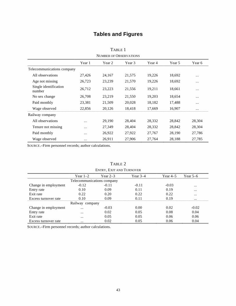
43
Tables and Figures
TABLE 1
NUMBER OF OBSERVATIONS
Year 1 Year 2 Year 3 Year 4 Year 5 Year 6 Telecommunications company
All observations 27,426 24,167 21,575 19,226 18,692 ... Age not missing 26,723 23,239 21,570 19,226 18,692 ... Single identification number 26,712 23,223 21,556 19,211 18,661 ...
No sex change 26,708 23,219 21,550 19,203 18,654 ... Paid monthly 23,381 21,509 20,028 18,182 17,488 ... Wage observed 22,856 20,126 18,418 17,669 16,907 ...
Railway company All observations ... 29,190 28,404 28,332 28,842 28,304 Tenure not missing ... 27,349 28,404 28,332 28,842 28,304 Paid monthly ... 26,922 27,922 27,767 28,190 27,786 Wage observed ... 26,911 27,906 27,764 28,188 27,785
SOURCE.–Firm personnel records; author calculations.
TABLE 2 ENTRY, EXIT AND TURNOVER
Year 1–2 Year 2–3 Year 3–4 Year 4–5 Year 5–6 Telecommunications company Change in employment -0.12 -0.11 -0.11 -0.03 ... Entry rate 0.10 0.09 0.11 0.19 ... Exit rate 0.22 0.20 0.22 0.22 ... Excess turnover rate 0.10 0.09 0.11 0.19 ... Railway company Change in employment ... -0.03 0.00 0.02 -0.02 Entry rate ... 0.02 0.05 0.08 0.04 Exit rate ... 0.05 0.05 0.06 0.06 Excess turnover rate ... 0.02 0.05 0.06 0.04
SOURCE.–Firm personnel records; author calculations.
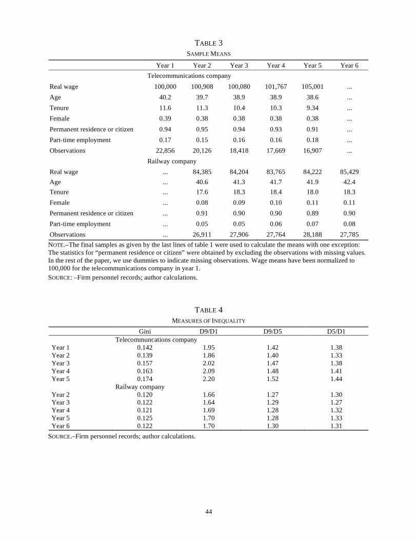
44
TABLE 3 SAMPLE MEANS
Year 1 Year 2 Year 3 Year 4 Year 5 Year 6 Telecommunications company Real wage 100,000 100,908 100,080 101,767 105,001 ... Age 40.2 39.7 38.9 38.9 38.6 ... Tenure 11.6 11.3 10.4 10.3 9.34 ... Female 0.39 0.38 0.38 0.38 0.38 ... Permanent residence or citizen 0.94 0.95 0.94 0.93 0.91 ... Part-time employment 0.17 0.15 0.16 0.16 0.18 ... Observations 22,856 20,126 18,418 17,669 16,907 ... Railway company Real wage ... 84,385 84,204 83,765 84,222 85,429 Age ... 40.6 41.3 41.7 41.9 42.4 Tenure ... 17.6 18.3 18.4 18.0 18.3 Female ... 0.08 0.09 0.10 0.11 0.11 Permanent residence or citizen ... 0.91 0.90 0.90 0.89 0.90 Part-time employment ... 0.05 0.05 0.06 0.07 0.08 Observations ... 26,911 27,906 27,764 28,188 27,785 NOTE.–The final samples as given by the last lines of table 1 were used to calculate the means with one exception: The statistics for “permanent residence or citizen” were obtained by excluding the observations with missing values. In the rest of the paper, we use dummies to indicate missing observations. Wage means have been normalized to 100,000 for the telecommunications company in year 1. SOURCE: –Firm personnel records; author calculations.
TABLE 4 MEASURES OF INEQUALITY
Gini D9/D1 D9/D5 D5/D1 Telecommuncations company Year 1 0.142 1.95 1.42 1.38 Year 2 0.139 1.86 1.40 1.33 Year 3 0.157 2.02 1.47 1.38 Year 4 0.163 2.09 1.48 1.41 Year 5 0.174 2.20 1.52 1.44 Railway company Year 2 0.120 1.66 1.27 1.30 Year 3 0.122 1.64 1.29 1.27 Year 4 0.121 1.69 1.28 1.32 Year 5 0.125 1.70 1.28 1.33 Year 6 0.122 1.70 1.30 1.31
SOURCE.–Firm personnel records; author calculations.

45
TABLE 5 LOG WAGE CHANGE DISTRIBUTIONS
Percentile Year 1–2 Wage Regime
Switch Year 2–3
Year 3–4 Year 4–5 Year 5–6
Telecommunications company 5 0.000 -0.149 0.000 0.015 ... 10 0.000 -0.080 0.016 0.015 ... 15 0.000 -0.036 0.018 0.015 ... 20 0.000 -0.026 0.019 0.016 ... 25 0.000 -0.020 0.021 0.019 ... 30 0.000 -0.017 0.022 0.022 ... 35 0.000 -0.010 0.024 0.024 ... 40 0.000 -0.002 0.025 0.027 ... 45 0.000 0.000 0.027 0.029 ... 50 0.000 0.001 0.030 0.032 ... 55 0.000 0.004 0.032 0.034 ... 60 0.000 0.013 0.034 0.037 ... 65 0.010 0.023 0.038 0.040 ... 70 0.023 0.033 0.042 0.044 ... 75 0.030 0.044 0.047 0.049 ... 80 0.034 0.058 0.055 0.055 ... 85 0.038 0.077 0.067 0.066 ... 90 0.042 0.098 0.088 0.081 ... 95 0.070 0.136 0.126 0.116 ... Std. dev. 0.034 0.086 0.042 0.038 Railway company 5 ... 0.000 -0.035 0.010 0.006 10 ... 0.000 0.000 0.010 0.007 15 ... 0.000 0.000 0.010 0.007 20 ... 0.000 0.000 0.010 0.007 25 ... 0.000 0.000 0.010 0.007 30 ... 0.000 0.000 0.010 0.007 35 ... 0.000 0.000 0.010 0.007 40 ... 0.000 0.000 0.010 0.007 45 ... 0.000 0.000 0.010 0.007 50 ... 0.000 0.000 0.010 0.007 55 ... 0.000 0.000 0.010 0.007 60 ... 0.000 0.000 0.027 0.020 65 ... 0.011 0.000 0.028 0.024 70 ... 0.022 0.007 0.031 0.025 75 ... 0.031 0.021 0.046 0.026 80 ... 0.039 0.036 0.050 0.043 85 ... 0.051 0.044 0.060 0.048 90 ... 0.063 0.057 0.080 0.067 95 ... 0.087 0.081 0.111 0.096 Std. dev. 0.039 0.041 0.039 0.034
NOTE.–The wage regime switch from the public to the private sector occurred for the telecommunications company between years 2 and 3. No change occurred in the railway company between those years. In the public-sector railway company, wage bargaining shifted from the national to the firm level between years 3 and 4. See also section IIB and the discussion of privatization versus decentralization effects in section VC. SOURCE.–Firm personnel records; author calculations.

46
TABLE 6 PRIVATIZATION EFFECTS
(1) (2) (3) Before-After Before-After Difference in Without Time Trend With Time Trend Differences Coef. S.E.. Coef. S.E. Coef. S.E. Constant -1.78 (0.29) -0.72 (0.39) -3.38 (0.32) Age (40–42)
Age: 18–27 7.46 (0.43) 2.11 (0.41) 2.16 (0.44) Age: 28–30 2.77 (0.44) 0.27 (0.40) 1.84 (0.40) Age: 31–33 1.84 (0.36) 0.44 (0.38) 0.89 (0.35) Age: 34–36 1.30 (0.22) 0.38 (0.30) 0.52 (0.30) Age: 37–39 0.84 (0.19) 0.24 (0.31) 0.33 (0.31) Age: 43–46 -0.81 (0.19) -0.39 (0.29) -0.11 (0.29) Age: 47–50 -1.63 (0.24) -0.98 (0.30) -0.80 (0.30) Age: 51–53 -2.24 (0.24) -1.44 (0.33) -1.24 (0.34) Age: 54–65 -4.14 (0.34) -3.09 (0.42) -2.72 (0.44)
Tenure (17–20) Tenure: 0–2 7.09 (0.48) 3.37 (0.60) 2.37 (1.74) Tenure: 3–5 5.21 (0.28) 2.70 (0.40) 2.50 (0.39) Tenure: 6–9 2.33 (0.27) 0.27 (0.36) 0.80 (0.30) Tenure: 10–11 0.96 (0.26) -0.80 (0.37) -0.17 (0.31) Tenure: 12–13 0.09 (0.38) -0.20 (0.37) 0.24 (0.34) Tenure: 14–16 0.83 (0.40) 0.30 (0.36) 0.54 (0.33) Tenure: 21–25 -0.23 (0.29) -0.39 (0.38) -0.38 (0.35) Tenure: 26–31 -0.24 (0.30) -0.24 (0.33) -0.21 (0.32) Tenure: 32–50 0.79 (0.50) 0.06 (0.61) 0.11 (0.64)
Skill (0.5–0.6) Skill: 0–0.1 3.23 (0.37) 1.45 (0.38) 2.60 (0.33) Skill: 0.1–0.2 1.01 (0.31) 0.26 (0.30) 0.64 (0.30) Skill: 0.2–0.3 -0.17 (0.31) -0.18 (0.30) 0.66 (0.30) Skill: 0.3–0.4 -0.55 (0.29) -0.39 (0.27) 0.39 (0.28) Skill: 0.4–0.5 -0.59 (0.28) -0.65 (0.27) 0.04 (0.27) Skill: 0.6–0.7 -0.01 (0.28) 0.04 (0.26) 0.46 (0.28) Skill: 0.7–0.8 0.71 (0.28) 0.26 (0.26) 0.71 (0.27) Skill: 0.8–0.9 0.93 (0.29) 0.40 (0.27) 0.66 (0.29) Skill: 0.9–1 2.31 (0.55) 1.58 (0.30) 1.31 (0.33)
Woman -3.86 (0.22) -2.32 (0.19) -2.80 (0.23) Nonpermanent visa 6.25 (2.45) 2.24 (1.89) 1.18 (1.10) Full-time (80–100) Part-time: 60–80 -5.16 (0.42) -3.20 (0.42) -2.24 (0.46) Part-time: 40–60 -5.65 (0.40) -3.17 (0.37) -2.07 (0.84) Part-time: 0–40 -13.24 (1.25) -7.23 (1.13) -10.71 (3.66) Number of obs. 75,462 75,462 157,095 R2 (within) 0.25 0.27 0.47
NOTE.–The dependent variable is the logged wage. Base categories are determined on the basis of the category into which the mean person of the telecommunications company falls in year 2. Robust standard errors allow for clustering and hence arbitrary autocorrelation within the wage growth observations of any person. All coefficients and standard errors have been multiplied by 100. Only the privatization effects (with the exception of the region coefficients) are reported. The coefficients on the levels of all variables, the time trends and the same variables for the railway firm are not reported but are available from the authors upon request. SOURCE.–Firm personnel records; author calculations.

47
TABLE 7 DYNAMICS OF THE PRIVATIZATION EFFECTS AND DECENTRALIZATION EFFECTS
(1) (2) (3) (4) Before-After With Before-After With Before-After With Before-After With Time Trend Time Trend Time Trend Time Trend Privatization 1 Y. After Priv. 2 Y. After Priv. Decentralization Coef. S.E. Coef. S.E. Coef. S.E. Coef. S.E. Constant -1.10 (0.33) 3.03 (0.29) 2.86 (0.48) -0.71 (0.07)
Age (40–42) Age: 18–27 3.10 (0.42) 2.21 (0.41) 1.87 (0.53) -0.17 (0.13) Age: 28–30 1.56 (0.61) 1.44 (0.63) 2.05 (0.70) -1.12 (0.10) Age: 31–33 0.64 (0.34) -0.54 (0.45) 0.59 (0.41) -0.30 (0.08) Age: 34–36 0.78 (0.29) 0.44 (0.26) 0.44 (0.28) -0.02 (0.07) Age: 37–39 0.43 (0.32) 0.05 (0.27) 0.32 (0.26) 0.00 (0.06) Age: 43–46 -0.57 (0.30) -0.33 (0.25) -0.11 (0.25) 0.05 (0.06) Age: 47–50 -1.10 (0.30) -0.32 (0.23) 0.04 (0.24) 0.08 (0.06) Age: 51–53 -1.58 (0.33) -0.34 (0.25) 0.10 (0.26) -0.01 (0.07)
Tenure (17–20) Tenure: 0–2 3.31 (0.55) ... ... ... ... 0.94 (0.74) Tenure: 3–5 3.39 (0.33) 0.67 (0.26) 0.91 (0.36) 0.42 (0.22) Tenure: 6–9 1.05 (0.30) 0.53 (0.23) 1.25 (0.32) -0.09 (0.10) Tenure: 10–11 -0.48 (0.32) 0.19 (0.25) 0.61 (0.32) -0.31 (0.08) Tenure: 12–13 0.15 (0.67) -0.16 (0.75) 0.66 (1.02) -0.02 (0.06) Tenure: 14–16 0.17 (0.35) -0.60 (0.45) 0.07 (0.51) 0.14 (0.06) Tenure: 21–25 -0.52 (0.37) -0.38 (0.26) 0.01 (0.35) 0.21 (0.06) Tenure: 26–31 -0.30 (0.30) -0.23 (0.23) -0.08 (0.30) -0.07 (0.06)
Skill (0.5–0.6) Skill: 0–0.1 0.62 (0.39) -0.69 (0.29) -1.34 (0.30) -0.48 (0.04) Skill: 0.1–0.2 0.11 (0.30) -0.01 (0.20) -0.31 (0.22) -0.40 (0.05) Skill: 0.2–0.3 -0.49 (0.30) -0.33 (0.21) -0.45 (0.23) -0.49 (0.05) Skill: 0.3–0.4 -0.64 (0.27) -0.09 (0.20) -0.40 (0.21) -0.27 (0.05) Skill: 0.4–0.5 -0.91 (0.26) -0.14 (0.18) -0.36 (0.21) -0.08 (0.05) Skill: 0.6–0.7 -0.05 (0.25) 0.18 (0.19) -0.24 (0.20) -0.11 (0.06) Skill: 0.7–0.8 0.23 (0.26) 0.11 (0.22) -0.02 (0.23) -0.09 (0.06) Skill: 0.8–0.9 0.36 (0.26) 0.16 (0.22) -0.08 (0.22) 0.08 (0.07) Skill: 0.9–1 1.64 (0.47) 0.11 (0.31) 0.10 (0.44) -0.33 (0.10)
Woman -2.19 (0.19) 0.11 (0.14) 0.18 (0.15) 0.24 (0.07) Nonpermanent visa 0.19 (1.66) -2.72 (3.38) -2.35 (2.61) 0.23 (0.16) Full-time (80–100) Part-time: 60–80 -3.26 (0.42) -0.23 (0.27) -0.01 (0.25) -0.21 (0.11) Part-time: 40–60 -3.45 (0.37) -0.19 (0.23) -0.54 (0.25) 0.40 (0.20) Part-time: 0–40 -7.54 (1.20) -0.36 (0.99) -0.54 (0.70) 1.51 (0.92) Number of obs. 75,462 124,288 R2 (within) 0.27 0.53 NOTE.–The dependent variable is the logged wage. Base categories are determined on the basis of the category into which the mean person of the telecommunications company falls in year 2. Because skill is proxied on the basis of the wage distribution in year 1, there are no persons in the sample with less than 2 years of tenure in years 4 and 5. Hence, no coefficients could be estimated for this group in columns 2 and 3. Robust standard errors allow for clustering and hence arbitrary autocorrelation within the wage growth observations of any person. All coefficients and standard errors have been multiplied by 100. Only the privatization or decentralization effects (with the exception of the region coefficients) are reported. The coefficients on the levels of all variables and the time trends are not reported but are available from the authors upon request. SOURCE.–Firm personnel records; author calculations.

48
TABLE 8 PRIVATIZATION EFFECTS ON EXIT FROM FIRM
(1) (2) Before-After Privatized Firm Difference Privatized-
Nonprivatized Firm Coef. S.E.. Coef. S.E. Constant 10.76 1.63 12.81 1.34 Age (40–42)
Age: 18–27 0.19 1.71 8.60 1.32 Age: 28–30 1.95 1.63 5.36 1.26 Age: 31–33 1.63 1.48 4.46 1.17 Age: 34–36 -0.37 1.38 1.52 1.09 Age: 37–39 -0.79 1.36 0.58 1.09 Age: 43–46 -2.46 1.36 -0.93 1.08 Age: 47–50 -2.27 1.43 -2.95 1.15 Age: 51–53 4.64 1.70 2.47 1.37 Age: 54–65 9.30 1.95 44.11 1.53
Tenure (17–20) Tenure: 0–2 -4.92 1.70 -0.90 1.26 Tenure: 3–5 -3.60 1.54 -0.13 1.20 Tenure: 6–9 -1.44 1.40 -1.77 1.14 Tenure: 10–11 -3.91 1.48 -5.44 1.16 Tenure: 12–13 -1.67 1.64 -2.03 1.21 Tenure: 14–16 -3.49 1.58 -2.73 1.27 Tenure: 21–25 -3.44 1.64 0.33 1.21 Tenure: 26–31 1.58 1.73 7.78 1.32 Tenure: 32–50 1.14 2.63 22.64 1.98
Skill (0.5–0.6) Skill: 0–0.1 7.99 1.52 9.63 1.29 Skill: 0.1–0.2 4.76 1.35 5.85 1.26 Skill: 0.2–0.3 4.88 1.31 7.82 1.24 Skill: 0.3–0.4 2.83 1.25 3.17 1.18 Skill: 0.4–0.5 0.19 1.20 0.82 1.13 Skill: 0.6–0.7 -3.95 1.15 -0.60 1.13 Skill: 0.7–0.8 -2.12 1.17 -2.21 1.10 Skill: 0.8–0.9 -3.73 1.16 -1.18 1.14 Skill: 0.9–1 -2.33 1.19 -1.03 1.18
Woman -3.95 0.92 -4.16 0.74 Nonpermanent visa -7.90 1.87 2.55 3.33 Full-time (80–100) Part-time: 60–80 -5.63 2.01 2.31 1.58 Part-time: 40–60 -13.92 1.87 0.34 1.40 Part-time: 0–40 -5.92 4.25 5.52 3.52 Number of obs. 39,427 45,036 R2 0.24 0.29
NOTE.– OLS regressions. The dependent variable is 1 if the person exits the firm and 0 if she stays in the firm. In column (1) the differences in the exits between waves 2 and 3 and between waves 1 and 2 are estimated for the privatized telecommunications firm. In column (2) the difference in the exits between the telecommunications and the railway firm between waves 2 and 3 are estimated. The reported privatization effects are the coefficients on the interactions between the original regressors and the wage regime change period (first column) or the privatized firm (second column). The coefficients on the levels of all variables (and on region) are not reported but are available from the authors. Robust standard errors allow for clustering and autocorrelation. All coefficients and standard errors have been multiplied by 100. SOURCE.–Firm personnel records; author calculations.

49
Real wage
Den
sity
Year 1Year 2Year 3Year 4Year 5
FIG. 1. –Real wage distributions: Telecommunications company NOTE.–Density of the real wage distribution estimated using a normal kernel. The same bandwidth has been used for each year and each firm. The scale of the axes has been masked for confidentiality reasons. SOURCE.–Firm personnel records; author calculations.

50
Real wage
Den
sity
Year 2Year 3Year 4Year 5Year 6
FIG. 2. –Real wage distributions: Railway company NOTE.–Density of the real wage distribution estimated using a normal kernel. The same bandwidth has been used for each year and each firm. The scale of the axes has been masked for confidentiality reasons. SOURCE.–Firm personnel records; author calculations.

51
Age group
Cha
nge
in lo
g w
age
-0.0
6-0
.04
-0.0
20.
000.
020.
040.
06
<28 31-33 37-39 43-46 51-53Tenure group
-0.0
20.
000.
020.
04
<=2 5-9 11-13 16-20 25-31
Skill group, defined by the conditional wage deciles
Cha
nge
in lo
g w
age
-0.0
2-0
.01
0.00
0.01
0.02
0-10 20-30 40-50 60-70 80-90Degree of employment
Rel
ativ
e lo
g w
age
grow
th
-0.1
5-0
.10
-0.0
5
0-40% 40-60% 60-80% 80-100%
FIG. 3.–Privatization effects using the before-after estimator without time trend
NOTE.–These results correspond to the first column of table 6. For each category, the displayed point estimate exhibits the privatization effect for an individual in this category with all other characteristics evaluated at the mean of the unconditional distribution. A 95 percent confidence interval is plotted using robust, individually clustered, standard errors. SOURCE.–Firm personnel records; author calculations.
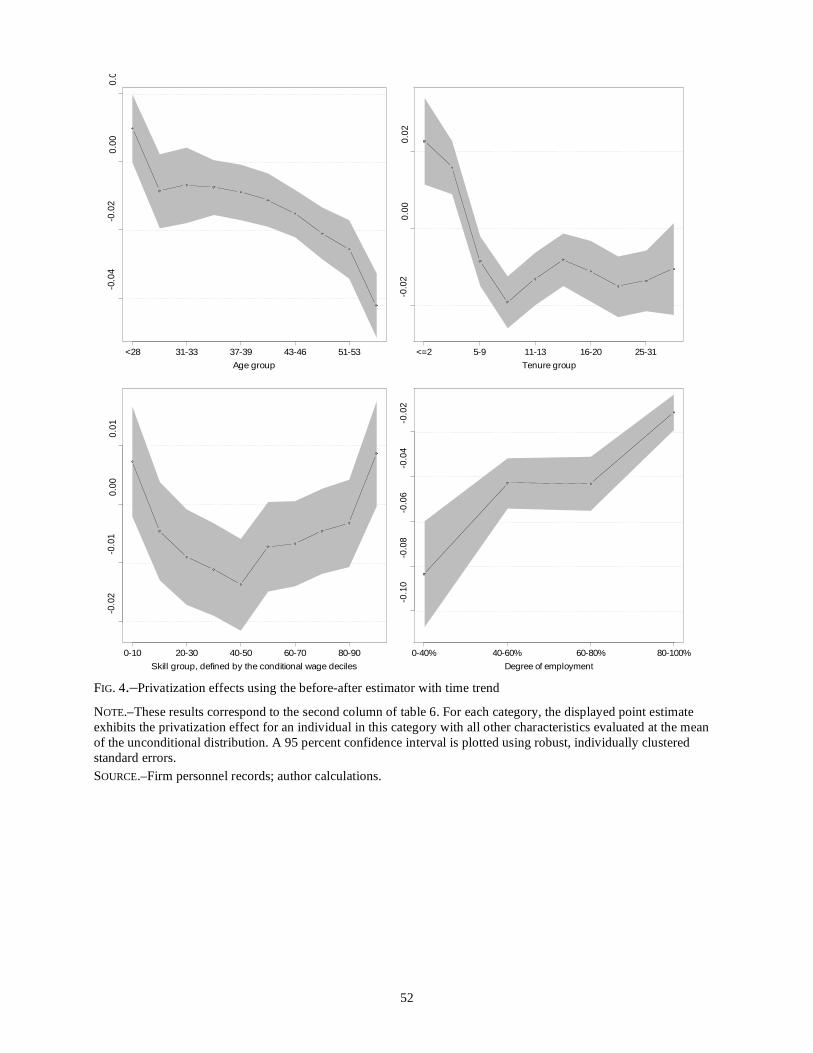
52
Age group
Cha
nge
in lo
g w
age
-0.0
4-0
.02
0.00
0.02
<28 31-33 37-39 43-46 51-53Tenure group
Rel
ativ
e lo
g w
age
grow
th
-0.0
20.
000.
02
<=2 5-9 11-13 16-20 25-31
Skill group, defined by the conditional wage deciles
Cha
nge
in lo
g w
age
-0.0
2-0
.01
0.00
0.01
0-10 20-30 40-50 60-70 80-90Degree of employment
Rel
ativ
e lo
g w
age
grow
th
-0.1
0-0
.08
-0.0
6-0
.04
-0.0
2
0-40% 40-60% 60-80% 80-100%
FIG. 4.–Privatization effects using the before-after estimator with time trend NOTE.–These results correspond to the second column of table 6. For each category, the displayed point estimate exhibits the privatization effect for an individual in this category with all other characteristics evaluated at the mean of the unconditional distribution. A 95 percent confidence interval is plotted using robust, individually clustered standard errors. SOURCE.–Firm personnel records; author calculations.

53
Age group
Cha
nge
in lo
g w
age
-0.0
6-0
.05
-0.0
4-0
.03
-0.0
2-0
.01
0.00
<28 31-33 37-39 43-46 51-53Tenure group
Rel
ativ
e lo
g w
age
grow
th
-0.0
4-0
.03
-0.0
2-0
.01
0.00
<=2 5-9 11-13 16-20 25-31
Skill group, defined by the conditional wage deciles
Cha
nge
in lo
g w
age
-0.0
4-0
.03
-0.0
2-0
.01
0.00
0-10 20-30 40-50 60-70 80-90Degree of employment
Rel
ativ
e lo
g w
age
grow
th
-0.2
0-0
.15
-0.1
0-0
.05
0-40% 40-60% 60-80% 80-100%
FIG. 5.–Privatization effects using the difference-in-differences estimator
NOTE.–These results correspond to the third column of table 6. For each category, the displayed point estimate exhibits the privatization effect for an individual in this category with all other characteristics evaluated at the mean of the unconditional distribution. A 95 percent confidence interval is plotted using robust, individually clustered standard errors. We have not plotted the results for the lowest tenure category, which is estimated very imprecisely because of the small number of observations in this group. SOURCE.–Firm personnel records; author calculations.

54
Age group
Rel
ative
log
wag
e gr
owth
-0.0
4-0
.02
0.00
0.02
0.04
<28 31-33 37-39 43-46 51-53
Privatization1 Year after privatization2 Years after privatization
Tenure group
-0.0
3-0
.02
-0.0
10.
000.
010.
020.
030.
04
<=2 5-9 11-13 16-20 25-31
Skill group, defined by the conditional wage deciles
Cha
nge
in lo
g w
age
-0.0
2-0
.01
0.00
0.01
0.02
0.03
0.04
0-10 20-30 40-50 60-70 80-90
Degree of employment
-0.1
0-0
.08
-0.0
6-0
.04
-0.0
20.
000.
02
80-100% 60-80% 40-60% 0-40%
FIG. 6.–Dynamics of the privatization effects
NOTE.–These results correspond to the first three columns of table 7. They have been computed using the before-after estimator with time trend. The point estimates are calculated in the same way as for figures 3, 4 ,and 5; that is, all other characteristics have been evaluated at their unconditional means to calculate the effects displayed. SOURCE.–Firm personnel records; author calculations.

55
Age group
Cha
nge
in lo
g w
age
-0.0
4-0
.02
0.00
0.02
<28 31-33 37-39 43-46 51-53
Tenure group
-0.0
20.
000.
02
<=2 5-9 11-13 16-20 25-31
Skill group, defined by the conditional wage deciles
Cha
nge
in lo
g w
age
-0.0
2-0
.01
0.00
0.01
0-10 20-30 40-50 60-70 80-90
Degree of employment
-0.0
8-0
.06
-0.0
4-0
.02
0.00
0.02
0-40% 40-60% 60-80% 80-100%
FIG. 7.–Decentralization of wage bargaining effects in the railway company
NOTE.–These results correspond to the last column of table 7. They have been computed using the before-after estimator with time trend. The point estimates are calculated in the same way as for figures 3, 4, and 5; that is, all other characteristics have been evaluated at their unconditional means to calculate the effects displayed. SOURCE.–Firm personnel records; author calculations.

56
Appendix A: Results for Stayers
TABLE A1 MEASURES OF INEQUALITY—FIVE-YEAR STAYERS ONLY
Gini D9/D1 D9/D5 D5/D1 Telecommuncations company Year 1 0.127 1.81 1.38 1.32 Year 2 0.133 1.77 1.38 1.28 Year 3 0.136 1.90 1.41 1.35 Year 4 0.138 1.89 1.41 1.34 Year 5 0.142 1.90 1.43 1.33 Railway company Year 2 0.115 1.61 1.26 1.28 Year 3 0.113 1.61 1.23 1.31 Year 4 0.111 1.61 1.23 1.31 Year 5 0.110 1.61 1.28 1.26 Year 6 0.109 1.59 1.28 1.24
NOTE.–Same calculations as for table 5 but using only the sample of five-year stayers. SOURCE.–Firm personnel records; author calculations.

57
Real wage
Den
sity
Year 1Year 2Year 3Year 4Year 5
FIG. A1.–Real wage distributions: Telecommunications company (five-year stayers only)
NOTE.–Same calculations as for figure 1 but using only the samples of five-year stayers. SOURCE.–Firm personnel records; author calculations.

58
Real wage
Den
sity
Year 2Year 3Year 4Year 5Year 6
FIG. A2.–Real wage distributions: Railway company (five-year stayers only)
NOTE.–Same calculations as for figure 2 but using only the samples of five-year stayers. SOURCE.–Firm personnel records; author calculations.

59
Age group
Rel
ativ
e lo
g w
age
grow
th
-0.0
4-0
.02
0.00
0.02
<28 31-33 37-39 43-46 51-53
AllOnly 5-year stayers
Tenure group-0
.02
0.00
0.02
<=2 5-9 11-13 16-20 25-31
Skill group, defined by the conditional wage deciles
Cha
nge
in lo
g w
age
-0.0
2-0
.01
0.00
0-10 20-30 40-50 60-70 80-90
Degree of employment
-0.1
2-0
.10
-0.0
8-0
.06
-0.0
4-0
.02
0-40% 40-60% 60-80% 80-100%
FIG. A3.–Privatization effects: All observations versus five-year stayers
NOTE.–The before-after estimator with time trend is applied using data for wears 1 to 3. A table with coefficients and standard errors is available upon request. SOURCE.–Firm personnel records; author calculations.