Proactive Online Scheduling for Shuffle Grouping in

Distributed Stream Processing Systems

Nicolo Rivetti, Emmanuelle Anceaume, Yann Busnel, Leonardo Querzoni,

Bruno Sericola

To cite this version:

Nicolo Rivetti, Emmanuelle Anceaume, Yann Busnel, Leonardo Querzoni, Bruno Sericola.Proactive Online Scheduling for Shuffle Grouping in Distributed Stream Processing Systems.[Research Report] LINA-University of Nantes; Sapienza Universita di Roma (Italie). 2015.<hal-01246701v2>

HAL Id: hal-01246701

https://hal.inria.fr/hal-01246701v2

Submitted on 4 Jan 2016

HAL is a multi-disciplinary open accessarchive for the deposit and dissemination of sci-entific research documents, whether they are pub-lished or not. The documents may come fromteaching and research institutions in France orabroad, or from public or private research centers.

L’archive ouverte pluridisciplinaire HAL, estdestinee au depot et a la diffusion de documentsscientifiques de niveau recherche, publies ou non,emanant des etablissements d’enseignement et derecherche francais ou etrangers, des laboratoirespublics ou prives.

1Proactive Online Schedulingfor Shuffle Grouping

in Distributed Stream Processing SystemsNicolo Rivetti∗§, Emmanuelle Anceaume†, Yann Busnel‡, Leonardo Querzoni§, Bruno Sericola¶

∗ LINA / Universite de Nantes, France - nicolo.rivetti@univ-nantes.fr† IRISA / CNRS, Rennes, France - emmanuelle.anceaume@irisa.fr‡ Crest (Ensai) / Inria, Rennes, France - yann.busnel@ensai.fr

§ DIAG / Sapienza University of Rome, Italy - {lastname}@dis.uniroma1.it¶Inria, Rennes, France - bruno.sericola@inria.fr

Abstract

Shuffle grouping is a technique used by stream processing frameworks to share input load among parallel instancesof stateless operators. With shuffle grouping each tuple of a stream can be assigned to any available operator instance,independently from any previous assignment. A common approach to implement shuffle grouping is to adopt around robin policy, a simple solution that fares well as long as the tuple execution time is constant. However, suchassumption rarely holds in real cases where execution time strongly depends on tuple content. As a consequence,parallel stateless operators within stream processing applications may experience unpredictable unbalance that, inthe end, causes undesirable increase in tuple completion times. In this paper we propose Proactive Online ShuffleGrouping (POSG), a novel approach to shuffle grouping aimed at reducing the overall tuple completion time. POSGestimates the execution time of each tuple, enabling a proactive and online scheduling of input load to the targetoperator instances. Sketches are used to efficiently store the otherwise large amount of information required to scheduleincoming load. We provide a probabilistic analysis and illustrate, through both simulations and a running prototype,its impact on stream processing applications.

I. INTRODUCTION

Stream processing systems are today gaining momentum as a tool to perform analytics on continuous data streams.Their ability to produce analysis results with sub-second latencies, coupled with their scalability, makes them thepreferred choice for many big data companies. A stream processing application is commonly modeled as a directacyclic graph where data operators, represented by vertices, are interconnected by streams of tuples containing datato be analyzed, the directed edges. Scalability is usually attained at the deployment phase where each data operatorcan be parallelized using multiple instances, each of which will handle a subset of the tuples conveyed by theoperator’s ingoing stream. The strategy used to route tuples in a stream toward available instances of the receivingoperator is embodied in a so-called grouping function.

Operator parallelization is straightforward for stateless operators, i.e., data operators whose output is only functionof the current tuple in input. In this case, in fact, the grouping function is free to assign the next tuple in the inputstream, to any available instance of the receiving operator (contrarily to statefull operators, where this choice istypically constrained). Such grouping functions are often called shuffle grouping.

Shuffle grouping implementations are designed to balance as much as possible the load on the receiving operatorinstances as this increases the system efficiency in available resource usage. Notable implementations [11] are basedon a simple Round-Robin assignment strategy that guarantees each operator instance will receive the same numberof input tuples. This approach is effective as long as the time taken by each operator instance to process a singletuple (tuple execution time) is the same for any incoming tuple. In this case, all parallel instances of the sameoperator will experience over time, on average, the same load.

This work was partially funded by the French ANR project SocioPlug (ANR-13-INFR-0003), and by the DeSceNt project granted by theLabex CominLabs excellence laboratory (ANR-10-LABX-07-01).

However, such assumption (i.e., same execution time for all tuples of a stream) does not hold for many practicaluse cases. The tuple execution time, in fact, may depend on the tuple content itself. This is often the case wheneverthe receiving operator implements a logic with branches where only a subset of the incoming tuples travels througheach single branch. If the computation associated with each branch generates different loads, then the executiontime will change from tuple to tuple. As a practical example consider an operator that works on a stream of inputtweets and that enriches them with historical data extracted from a database, where this historical data is added onlyto tweets that contain specific hashtags: only tuples that get enriched require an access to the database, an operationthat typically introduces non negligible latencies at execution time. In this case shuffle grouping implemented withRound-Robin, may produce imbalance between the operator instances, and this typically causes an increase in thetime needed for a tuple to be completely processed by the application (tuple completion time) as some tuple mayend-up being queued on some overloaded operator instances, while other instances are available for immediateprocessing.

In this paper we introduce Proactive Online Shuffle Grouping (POSG) a novel approach to shuffle grouping thataims at reducing tuple completion times by accurately scheduling incoming tuples on available operator instancesin order to avoid imbalances. To the best of our knowledge POSG is the first solution that explicitly addresses andsolves the above stated problem.

The idea at the basis of POSG is simple: by measuring the amount needed by operator instances to processeach tuple we can schedule incoming tuples minimizing the completion time. However, making such idea works inpractice in a streaming setting is not trivial. In particular, POSG makes use of sketches to efficiently keep track ofthe huge amount of information related to tuple execution times and then applies a greedy online multiprocessorscheduling algorithm to assign tuples to operator instances at runtime. The status of each instance is monitored ina smart way in order to detect possible changes in the input load distribution and coherently adapt the scheduling.As a result, POSG provides an important performance gain in terms of tuple completion times with respect toRound-Robin for all those settings where tuple processing times are not constant, but rather depend on the tuplecontent.

In summary, we provide the following contributions:• we introduce POSG the first solution for shuffle grouping that explicitly addresses the problem of parallel

operator instances imbalance under loads characterized by non-uniform tuple execution times; POSG schedulestuple on target operator instances online, with minimal resource usage; it works at runtime and is able tocontinuously adapt to changes in the input load;

• We study the two components of our solution: (i) showing that the scheduling algorithm efficiently approximatethe optimal one and (ii) providing some error bounds as well as a probabilistic analysis of the accuracy of thetuple execution time tracking algorithm;

• we evaluate POSG’s sensibility to both the load characteristic and its configuration parameters with an extensivesimulation-based evaluation that points the scenarios where POSG is expected to provide its best performance;

• we evaluate POSG’s performance by integrating a prototype implementation with the Apache Storm streamprocessing framework on Microsoft Azure platform and running it on a real dataset.

After this introduction, the paper starts by defining a system model and stating the problem we intend to attack(Section II); it then introduces POSG (Section III) and shows the results of our probabilistic analysis (Section IV);results from our experimental campaign are reported in Section V and are followed by a discussion of the relatedworks (Section VI); finally, Section VII concludes the paper.

II. SYSTEM MODEL

We consider a distributed stream processing system (SPS) deployed on a cluster where several computing nodesexchange data through messages sent over a network. The SPS executes a stream processing application representedby a topology: a direct acyclic graph interconnecting operators, represented by nodes, with data streams (DS),represented by edges. Each topology contains at least a source, i.e., an operator connected only through outboundDSs, and a sink, i.e., an operator connected only through inbound DSs. Each operator O can be parallelizedby creating k independent instances O0, · · · , Ok−1 of it and by partitioning its inbound stream Oin in k sub-streams Oin0 , · · · , Oink−1. Tuples are assigned to sub-streams with a grouping function. Several grouping strategiesare available, but in this work we restrict our analysis to shuffle grouping where each incoming tuple can be assignedto any sub-stream.

2

Data injected by the source is encapsulated in units called tuples and each data stream is an unbounded sequenceof tuples. Without loss of generality, here we assume that each tuple t is a finite set of key/value pairs that canbe customized to represent complex data structures. To simplify the discussion, in the rest of this work we dealwith streams of unary tuples with a single non negative integer value. For the sake of clarity, and without loss ofgenerality, here we restrict our model to a topology with an operator S (scheduler) which schedules the tuples ofa DS Oin consumed by the instances O0, · · · , Ok−1 of operator O.

We denote as wt,i the execution time of tuple t on operator instance Oi. Abusing the notation, we may omitthe instance identifier subscript. We assume that the execution time wt,i depends on the content of the tuple t:wt,i = gi(t), where gi is an unknown function that may be different for each operator instance. We simplify themodel assuming that the functions gi(t) depend on a single fixed and known attribute value of t. The probabilitydistribution of such attribute values, as well as the functions gi(t) are unknown and may change over time. However,we assume that subsequent changes are interleaved by a large enough time frame such that an algorithm may havea reasonable amount of time to adapt.

Let l(i) be the completion time of the i-th tuple of the stream, i.e., the time it takes for the i-th tuple from themoment it is injected by the source in the topology, till the moment the last operator concludes processing it. Thenwe can define the average completion time as: L =

∑i∈[m] l(i)/m.

The general goal we target in this work is to minimize the average tuple completion time L. Such metric isfundamentally driven by three factors: (i) tuple execution times at operator instances, (ii) network latencies and (iii)queuing delays. More in detail, we aim at reducing queuing delays at parallel operator instances that receive inputtuples through shuffle grouping.

Typical implementation of shuffle grouping are based on Round-Robin scheduling. However, this tuple to DSsub-streams assignment strategy may introduce additional queuing delays when the execution time of input tuplesis not constant. For instance, let a0, b1, a2 be a stream with an inter tuple arrival delay of 1s, where a and b aretuples with the following execution time: wa = 10s and wb = 1s. Scheduling this stream with Round-Robin onk = 2 operator instances would assign a0 and a2 to instance 1 and b1 to instance 2, with a cumulated completiontime equal to 10+1+10+(10−2) = 29s (i.e., 8s wasted for the additional queuing delay of a2). A better schedulewould be to assign a0 to instance 1, while b1 and a2 to instance 2. In this case, the cumulated completion timeequals to 10 + 1 + 10 = 21s (i.e., no queuing delay).

III. PROACTIVE ONLINE SHUFFLE GROUPING

Proactive Online Shuffle Grouping is a shuffle grouping implementation based on a simple, yet effective idea: ifwe assume to know the execution time wt,i of each tuple t on the available operator instances O0, · · · , Ok−1, wecan schedule the execution of incoming tuples on such instances with the aim of minimizing the average per tuplecompletion time at the operator instances. However, the value of wt,i is generally unknown. A common solutionto this problem is to build a cost model for tuple execution and then use it to proactively schedule incomingload. However building an accurate cost model usually requires a large amount of a priori knowledge on thesystem. Furthermore, once a model has been built, it can be hard to handle changes in the system or input streamcharacteristics at runtime. Another common alternative is to periodically collect at the scheduler the load of theoperator instances. However, this solution only allows for reactive scheduling, where input tuples are scheduled onthe basis of a previous, possibly stale, load state of the operator instances; reactive scheduling typically impose aperiodic overhead even if the load distribution imposed by input tuples does not change over time.

To overcome all these issues, POSG takes decision based on the estimation Ci of the execution time assigned toinstance i: Ci =

∑∀t∈Oin

iwt,i. In order to do so, POSG computes an estimation wt,i of the execution time wt,i of

each tuple t on each operator instance i. Then, POSG can also compute the sum of the estimated execution timesof the tuples assigned to an instance i, i.e., Ci =

∑∀t∈Oin

iwt,i, which in turn is the estimation of Ci. A greedy

scheduling algorithm (Section III-A) is then fed with estimations for all the available operator instances. To enablethis approach, each operator instance builds a sketch (i.e., a memory efficient data structure) that will track theexecution time of the tuples it process. When a change in the stream or instance(s) characteristics affects the tuplesexecution times on some instances, the concerned instance(s) will forward an updated sketch to the scheduler whichwill than be able to (again) correctly estimate the tuples execution times. This solution does not require any a prioriknowledge on the stream or system, and is designed to continuously adapt to changes in the input distribution or

3

on the instances load characteristics. In addition, this solution is proactive, namely its goal is to avoid unbalancethrough scheduling, rather than detecting the unbalance and then attempting to correct it.

A. Background

Data Streaming model — We present the data stream model [9], under which we analyze our algorithms andderive bounds. A stream is an unbounded sequence of elements σ = 〈t1, . . . , tm〉 called tuples or items, which aredrawn from a large universe [n] = {1, . . . , n}. The unknown size (or length) of the stream is denoted by m. Wedenote by pt the unknown probability of occurrence of item t in the stream and with ft the unknown frequency1

of item t, i.e., the number of occurrences of t in the stream of size m.

2-Universal Hash Functions — Our algorithm uses hash functions randomly picked from a 2-universal hashfunctions family. A collection H of hash functions h : {1, . . . , n} → {0, . . . , c} is said to be 2-universal if for everytwo different items x, y ∈ [n], for all h ∈ H, P{h(x) = h(y)} ≤ 1

c , which is the probability of collision obtained ifthe hash function assigned truly random values to any x ∈ [c]. Carter and Wegman [4] provide an efficient methodto build large families of hash functions approximating the 2-universality property.

Count Min sketch algorithm — Cormode and Muthukrishnan have introduced in [5] the Count Min sketchthat provides, for each item t in the input stream an (ε, δ)-additive-approximation ft of the frequency ft. TheCount Min sketch consists of a two dimensional matrix F of size r × c, where r =

⌈log 1

δ

⌉and c =

⌈eε

⌉. Each

row is associated with a different 2-universal hash function hi : [n]→ [c]. When the Count Min algorithm readssample t from the input stream, it updates each row: ∀i ∈ [r],F [i, hi(t)] ← F [i, hi(t)] + 1. Thus, the cell valueis the sum of the frequencies of all the items mapped to that cell. Upon request of ft estimation, the algorithmreturns the smallest cell value among the cell associated with t: ft = mini∈[r]{F [i, hi(t)]}.

Fed with a stream of m items, the space complexity of this algorithm is O( 1ε log 1

δ (logm + log n)) bits, whileupdate and query time complexities are O(log 1/δ). The Count Min algorithm guarantees that the followingbound holds on the estimation accuracy for each iteam read from the input stream: P{| ft− ft |≥ ε(m− ft)} ≤ δ,while ft ≤ ft is always true.

This algorithm can be easily generalized to provide (ε, δ)-additive-approximation of point queries Qt on streamof udpates, i.e., a stream where each item t carries a positive integer update value vt. When the Count Minalgorithm reads the pair 〈t, vt〉 from the input stream, the update routine changes as follows: ∀i ∈ [r],F [i, hi(t)]←F [i, hi(t)] + vt.

Greedy Online Scheduler — A classical problem in the load balancing literature is to schedule independent taskson identical machines minimizing the makespan, i.e., the Multiprocessor Scheduling problem. In this paper we adaptthis problem to our setting, i.e., to schedule online independent tasks on non uniform machines aiming to minimizingthe average per task completion time L. Online scheduling means that the scheduler does not know in advancethe sequence of tasks it has to schedule. The Greedy Online Scheduler algorithm assigns the currently submittedtasks to the less loaded available machine. In Section IV-A we prove that this algorithm closely approximates theoptimal algorithm.

B. POSG design

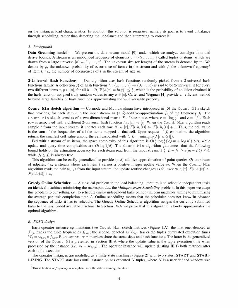
Each operator instance op maintains two Count Min sketch matrices (Figure 1.A): the first one, denoted asFop, tracks the tuple frequencies ft,op; the second, denoted as Wop, tracks the tuples cumulated execution timesWt = wt,op×ft,op. Both Count Min matrices share the same sizes and hash functions. The latter is the generalizedversion of the Count Min presented in Section III-A where the update value is the tuple execution time whenprocessed by the instance (i.e., vt = wt,op) . The operator instance will update (Listing III.1) both matrices aftereach tuple execution.

The operator instances are modelled as a finite state machines (Figure 2) with two states: START and STABI-LIZING. The START state lasts until instance op has executed N tuples, where N is a user defined window size

1This definition of frequency is compliant with the data streaming literature.

4

c1 2 3 4

r2

1

FO2

c1 2 3 4

WO2

〈FO2,WO2

〉

O2

〈FO1 ,WO1〉

O1

POSG

C = [CO1, CO2

]

〈FO1,WO1

〉

〈FO2,WO2

〉

S

〈tuple〉| 〈tupl

e, C[O1]〉

〈FO2,WO2

〉

〈∆O2 〉

A

B

C

D

E

Fig. 1. Proactive Online Shuffle Grouping design with r = 2 (δ = 0.25), c = 4 (ε = 0.70) and k = 2.

Listing III.1: Operator instance op: update Fop and Wop.1: init do2: Fop matrix of size r × c3: Wop matrix of size r × c4: r hash functions h1 . . . hr : [n]→ [c] from a 2-universal family (same for all instances).5: end init6: function UPDATE(tuple : t, execution time : l)7: for i = 1 to c do8: Fop[i, hi(t)]← Fop[i, hi(t)] + 19: Wop[i, hi(t)]←Wop[i, hi(t)] + l

10: end for11: end function

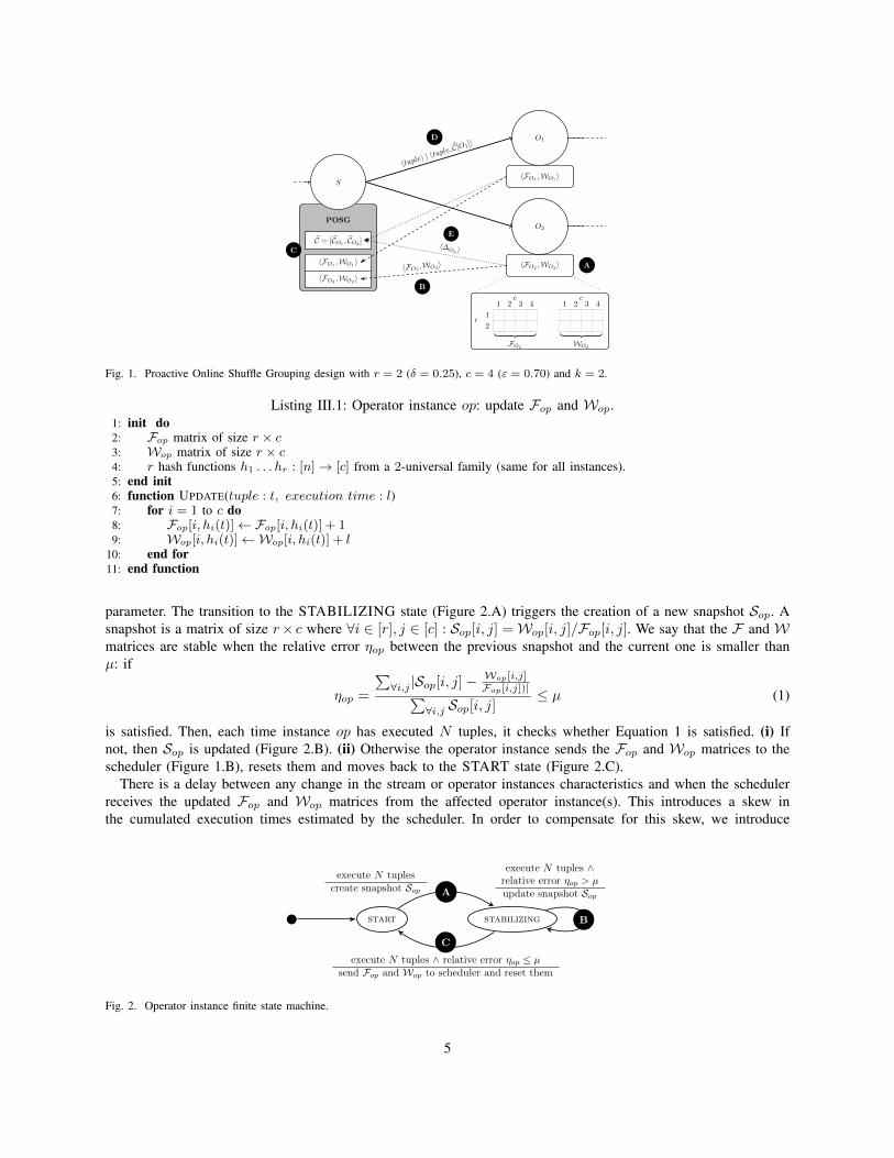
parameter. The transition to the STABILIZING state (Figure 2.A) triggers the creation of a new snapshot Sop. Asnapshot is a matrix of size r× c where ∀i ∈ [r], j ∈ [c] : Sop[i, j] =Wop[i, j]/Fop[i, j]. We say that the F and Wmatrices are stable when the relative error ηop between the previous snapshot and the current one is smaller thanµ: if

ηop =

∑∀i,j |Sop[i, j]−

Wop[i,j]Fop[i,j])|∑

∀i,j Sop[i, j]≤ µ (1)

is satisfied. Then, each time instance op has executed N tuples, it checks whether Equation 1 is satisfied. (i) Ifnot, then Sop is updated (Figure 2.B). (ii) Otherwise the operator instance sends the Fop and Wop matrices to thescheduler (Figure 1.B), resets them and moves back to the START state (Figure 2.C).

There is a delay between any change in the stream or operator instances characteristics and when the schedulerreceives the updated Fop and Wop matrices from the affected operator instance(s). This introduces a skew inthe cumulated execution times estimated by the scheduler. In order to compensate for this skew, we introduce

start stabilizing

execute N tuplescreate snapshot Sop

execute N tuples ∧ relative error ηop ≤ µsend Fop and Wop to scheduler and reset them

execute N tuples ∧relative error ηop > µupdate snapshot SopA

B

C

Fig. 2. Operator instance finite state machine.

5

a synchronization mechanism that kicks in whenever the scheduler receives a new pair of matrices from anyoperator instance. Notice also that there is an initial transient phase in which the scheduler has not yet receivedany information from operator instances. This means that in this first phase it has no information on the tuplesexecution times and is forced to use the Round-Robin policy. This mechanism is thus also needed to initialize theestimated cumulated execution times when the Round-Robin phase ends.

RoundRobin

WaitAll

SendAll

Run

receive new Fop and Wop

add to {〈Fop,Wop〉} set

received Fop and Wop

from eachoperator instance

synhcronization requestssent to each operator instance

received reply

received all replies

resynchronize C

receive udpatedFop and Wop

update local Fop and Wop

AB

C

D

E

F

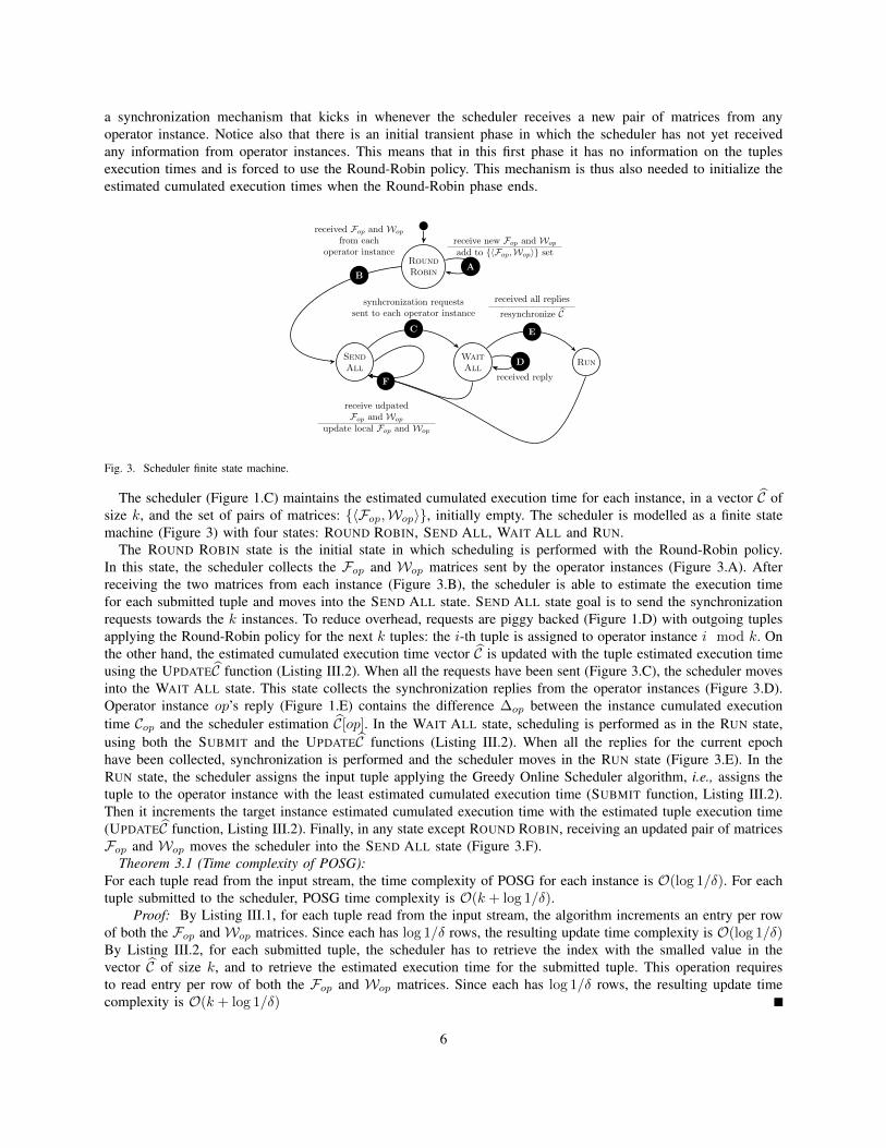
Fig. 3. Scheduler finite state machine.

The scheduler (Figure 1.C) maintains the estimated cumulated execution time for each instance, in a vector C ofsize k, and the set of pairs of matrices: {〈Fop,Wop〉}, initially empty. The scheduler is modelled as a finite statemachine (Figure 3) with four states: ROUND ROBIN, SEND ALL, WAIT ALL and RUN.

The ROUND ROBIN state is the initial state in which scheduling is performed with the Round-Robin policy.In this state, the scheduler collects the Fop and Wop matrices sent by the operator instances (Figure 3.A). Afterreceiving the two matrices from each instance (Figure 3.B), the scheduler is able to estimate the execution timefor each submitted tuple and moves into the SEND ALL state. SEND ALL state goal is to send the synchronizationrequests towards the k instances. To reduce overhead, requests are piggy backed (Figure 1.D) with outgoing tuplesapplying the Round-Robin policy for the next k tuples: the i-th tuple is assigned to operator instance i mod k. Onthe other hand, the estimated cumulated execution time vector C is updated with the tuple estimated execution timeusing the UPDATEC function (Listing III.2). When all the requests have been sent (Figure 3.C), the scheduler movesinto the WAIT ALL state. This state collects the synchronization replies from the operator instances (Figure 3.D).Operator instance op’s reply (Figure 1.E) contains the difference ∆op between the instance cumulated executiontime Cop and the scheduler estimation C[op]. In the WAIT ALL state, scheduling is performed as in the RUN state,using both the SUBMIT and the UPDATEC functions (Listing III.2). When all the replies for the current epochhave been collected, synchronization is performed and the scheduler moves in the RUN state (Figure 3.E). In theRUN state, the scheduler assigns the input tuple applying the Greedy Online Scheduler algorithm, i.e., assigns thetuple to the operator instance with the least estimated cumulated execution time (SUBMIT function, Listing III.2).Then it increments the target instance estimated cumulated execution time with the estimated tuple execution time(UPDATEC function, Listing III.2). Finally, in any state except ROUND ROBIN, receiving an updated pair of matricesFop and Wop moves the scheduler into the SEND ALL state (Figure 3.F).

Theorem 3.1 (Time complexity of POSG):For each tuple read from the input stream, the time complexity of POSG for each instance is O(log 1/δ). For eachtuple submitted to the scheduler, POSG time complexity is O(k + log 1/δ).

Proof: By Listing III.1, for each tuple read from the input stream, the algorithm increments an entry per rowof both the Fop andWop matrices. Since each has log 1/δ rows, the resulting update time complexity is O(log 1/δ)By Listing III.2, for each submitted tuple, the scheduler has to retrieve the index with the smalled value in thevector C of size k, and to retrieve the estimated execution time for the submitted tuple. This operation requiresto read entry per row of both the Fop and Wop matrices. Since each has log 1/δ rows, the resulting update timecomplexity is O(k + log 1/δ)

6

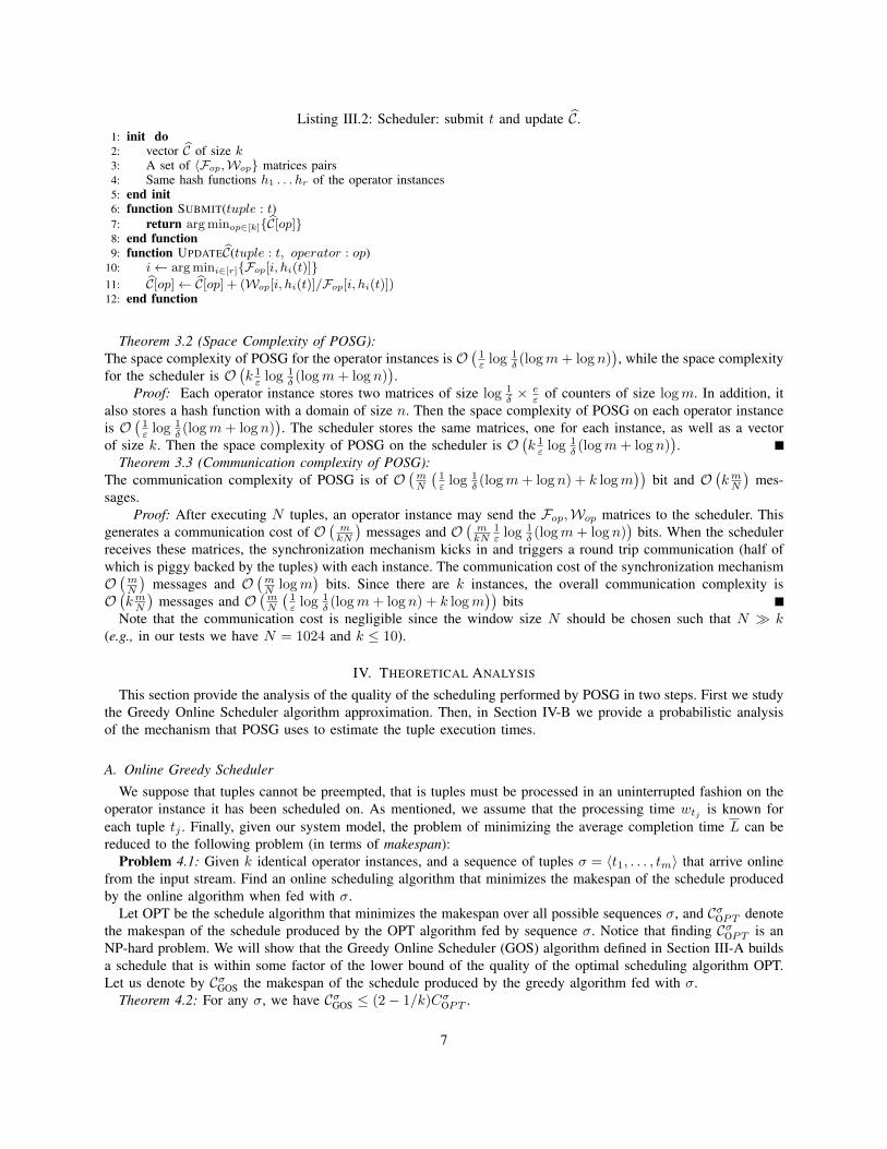
Listing III.2: Scheduler: submit t and update C.1: init do2: vector C of size k3: A set of 〈Fop,Wop} matrices pairs4: Same hash functions h1 . . . hr of the operator instances5: end init6: function SUBMIT(tuple : t)7: return argminop∈[k]{C[op]}8: end function9: function UPDATEC(tuple : t, operator : op)

10: i← argmini∈[r]{Fop[i, hi(t)]}11: C[op]← C[op] + (Wop[i, hi(t)]/Fop[i, hi(t)])12: end function

Theorem 3.2 (Space Complexity of POSG):The space complexity of POSG for the operator instances is O

(1ε log 1

δ (logm+ log n)), while the space complexity

for the scheduler is O(k 1ε log 1

δ (logm+ log n)).

Proof: Each operator instance stores two matrices of size log 1δ × e

ε of counters of size logm. In addition, italso stores a hash function with a domain of size n. Then the space complexity of POSG on each operator instanceis O

(1ε log 1

δ (logm+ log n)). The scheduler stores the same matrices, one for each instance, as well as a vector

of size k. Then the space complexity of POSG on the scheduler is O(k 1ε log 1

δ (logm+ log n)).

Theorem 3.3 (Communication complexity of POSG):The communication complexity of POSG is of O

(mN

(1ε log 1

δ (logm+ log n) + k logm))

bit and O(kmN)

mes-sages.

Proof: After executing N tuples, an operator instance may send the Fop,Wop matrices to the scheduler. Thisgenerates a communication cost of O

(mkN

)messages and O

(mkN

1ε log 1

δ (logm+ log n))

bits. When the schedulerreceives these matrices, the synchronization mechanism kicks in and triggers a round trip communication (half ofwhich is piggy backed by the tuples) with each instance. The communication cost of the synchronization mechanismO(mN

)messages and O

(mN logm

)bits. Since there are k instances, the overall communication complexity is

O(kmN)

messages and O(mN

(1ε log 1

δ (logm+ log n) + k logm))

bitsNote that the communication cost is negligible since the window size N should be chosen such that N � k

(e.g., in our tests we have N = 1024 and k ≤ 10).

IV. THEORETICAL ANALYSIS

This section provide the analysis of the quality of the scheduling performed by POSG in two steps. First we studythe Greedy Online Scheduler algorithm approximation. Then, in Section IV-B we provide a probabilistic analysisof the mechanism that POSG uses to estimate the tuple execution times.

A. Online Greedy Scheduler

We suppose that tuples cannot be preempted, that is tuples must be processed in an uninterrupted fashion on theoperator instance it has been scheduled on. As mentioned, we assume that the processing time wtj is known foreach tuple tj . Finally, given our system model, the problem of minimizing the average completion time L can bereduced to the following problem (in terms of makespan):

Problem 4.1: Given k identical operator instances, and a sequence of tuples σ = 〈t1, . . . , tm〉 that arrive onlinefrom the input stream. Find an online scheduling algorithm that minimizes the makespan of the schedule producedby the online algorithm when fed with σ.

Let OPT be the schedule algorithm that minimizes the makespan over all possible sequences σ, and CσOPT denotethe makespan of the schedule produced by the OPT algorithm fed by sequence σ. Notice that finding CσOPT is anNP-hard problem. We will show that the Greedy Online Scheduler (GOS) algorithm defined in Section III-A buildsa schedule that is within some factor of the lower bound of the quality of the optimal scheduling algorithm OPT.Let us denote by CσGOS the makespan of the schedule produced by the greedy algorithm fed with σ.

Theorem 4.2: For any σ, we have CσGOS ≤ (2− 1/k)CσOPT .

7

Proof: Let i ∈ [k] be the instance on which the last tuple tj is executed. By construction of the algorithm,when tuple tj starts its execution on instance i, all the other instances are busy, otherwise tj would have beenexecuted on another instance. Thus when tuple tj starts its execution on instance i, each of the k instances musthave been allocated a load at least equivalent to (

∑m`=1 wt` − wtj )/k. Thus we have,

CσGOS − wtj ≤∑m`=1 wt` − wtj

k

CσGOS ≤∑m`=1 wt`k

+ wtj (1− 1

k) (2)

Now, it is easy to see that

CσOPT ≥∑mj=1 wtj

k, (3)

otherwise the total load processed by all the machines in the schedule produced by the OPT algorithm would bestrictly less than

∑mj=1 wtj , leading to a contradiction. We also trivially have

CσOPT ≥ max`wt` . (4)

Thus combining relations (2), (3), and (4), we have

CσGOS ≤ CσOPT + CσOPT (1− 1

k)

= (2− 1

k)CσOPT (5)

that concludes the proof.This lower bound is tight, that is there are sequences of tuples for which the Greedy Online Scheduler algorithm

produces a schedule whose completion time is exactly equal to (2− 1/k) times the completion time of the optimalscheduling algorithm [7].

Consider the example of a(a−1) tuples whose processing time is equal to wmax/k and one task with a processingtime equal to wmax. Suppose that the a(a− 1) tuples are scheduled first and then the longest one. Then the greedyalgorithm will exhibit a makespan equal to (m− 1)wmax/k + wmax = wmax(2− 1/k) while the OPT schedulingwill lead to a makespan equal to wmax.

B. Execution Time Estimation

POSG uses two matrices, F and W , to estimate the execution time wt of each tuple submitted to the scheduler.To simplify the discussion, we consider a single operator instance.

From the count Min algorithm, and for any v ∈ {1, . . . , n}, we have for a given hash function hi,

Cv(m) =

n∑

u=1

fu1{hi(u)=hi(v)} = fv +

n∑

u=1,u 6=v

fu1{hi(u)=hi(v)}.

and

Wv(m) = fvwv +

n∑

u=1,u6=v

fuwu1{hi(u)=hi(v)},

where Cv(m) = F [v][hv(m)] and Wv(m) = W[v][hv(m)]. Let us denote respectively by wmin and wmax theminimum and the maximum execution time of the items. We have trivially

wmin ≤Wv(m)

Cv(m)≤ wmax.

In the following we write respectively Cv and Wv instead of Cv(m) and Wv(m), to simplify the writing. For anyi = 0, . . . , n− 1, we denote by Ui(v) the set which elements are the subsets {1, . . . , n} \ {v} whose size is equalto i, that is

Ui(v) = {A ⊆ {1, . . . , n} \ {v} | |A| = i}.

8

We have U0(v) = {∅}.For any v = 1, . . . , n, i = 0, . . . , n− 1 and A ∈ Ui(v), we introduce the event B(v, i, A) defined by

B(v, i, A) = {hu = hv, ∀u ∈ A and hu 6= hv, ∀u ∈ {1, . . . , n} \ (A ∪ {v})} .From the independence of the hu, we have

Pr{B(v, i, A)} =

(1

k

)i(1− 1

k

)n−1−i.

Let us consider the ratio Wv/Cv . For any i = 0, . . . , n, we define

Ri(v) =

{fvwv +

∑u∈A fuwu

fv +∑u∈A fu

, A ∈ Ui(v)

}.

We have R0(v) = {wv}. We introduce the set R(v) defined by

R(v) =

n−1⋃

i=0

Ri(v).

Thus with probability 1,Wv/Cv ∈ R(v).

Let x ∈ R(v). We have

Pr{Wv/Cv = x} =

n−1∑

i=0

∑

A∈Ui(v)

Pr{Wv/Cv = x | B(v, i, A)}Pr{B(v, i, A)}

=

n−1∑

i=0

(1

k

)i(1− 1

k

)n−1−i ∑

A∈Ui(v)

Pr{Wv/Cv = x | B(v, i, A)}

=

n−1∑

i=0

(1

k

)i(1− 1

k

)n−1−i ∑

A∈Ui(v)

1{x=(fvwv+∑

u∈A fuwu)/(fv+∑

u∈A fu)}.

Thus

E{Wv/Cv} =

n−1∑

i=0

(1

k

)i(1− 1

k

)n−1−i ∑

A∈Ui(v)

∑

x∈R(v)

x1{x=(fvwv+∑

u∈A fuwu)/(fv+∑

u∈A fu)}

=

n−1∑

i=0

(1

k

)i(1− 1

k

)n−1−i ∑

A∈Ui(v)

fvwv +∑u∈A fuwu

fv +∑u∈A fu

∑

x∈R(v)

1{x=(fvwv+∑

u∈A fuwu)/(fv+∑

u∈A fu)}

=

n−1∑

i=0

(1

k

)i(1− 1

k

)n−1−i ∑

A∈Ui(v)

fvwv +∑u∈A fuwu

fv +∑u∈A fu

.

Let us assume that all the fu are equal, that is for each u, we have fu = m/n. Simulations tend to show thatthe worst cases scenario of input streams are exhibited when all the items show the same number of occurrencesin the input stream. We get

Pr{Wv/Cv = x} =

n−1∑

i=0

(1

k

)i(1− 1

k

)n−1−i ∑

A∈Ui(v)

1{x=(wv+∑

u∈A wu)/(i+1)}.

We define S =∑ni=1 wi. We then have

Theorem 4.3:

E{Wv/Cv} =S − wvn− 1

− k(S − nwv)n(n− 1)

(1−

(1− 1

k

)n).

It important to note that this result does not depend on m.

9

Let us now consider a numerical application. We take k = 55, n = 4096 and the distinct values of wu equalto 1, 2, 3, . . . , 64, each item being present 64 times in the input stream, we get for v = 1, . . . , 64, E{Wv/Cv} ∈[32.08, 32.92]. Note also from above that we have 1 ≤Wv/Cv ≤ 64.

From the Markov inequality we have, for every x > 0,

Pr{Wv/Cv ≥ x} ≤E{Wv/Cv}

x.

By taking x = 64a, with a ∈ [0.6, 1), we obtain

Pr{Wv/Cv ≥ 64a} ≤ E{Wv/Cv}64a

≤ 33

64a.

If r denotes the number of rows of the system, we have by the independence of the h functions,

Pr{ mint=1,...,r

(Wt,v/Ct,v) ≥ 64a} = (Pr{Wv/Cv ≥ 64a})r ≤(

33

64a

)r.

By taking for instance a = 3/4 and r = 10, we get

Pr{ mint=1,...,r

(Wt,v/Ct,v) ≥ 48} ≤(

11

16

)10

≤ 0.024.

V. EXPERIMENTAL EVALUATION

In this section we evaluate the performance obtained by using POSG to perform shuffle grouping. We will firstdescribe the general setting used to run the tests and will then discuss the results obtained through simulations(Section V-B) and with a prototype of POSG targeting Apache Storm (Section V-C).

A. Setup

Datasets — In our tests we consider both synthetic and real datasets. For synthetic datasets we generate streams ofinteger values (items) representing the values of the tuple attribute driving the execution time when processed on anoperator instance. We consider streams of m = 32, 768 tuples, each containing a value chosen among n = 4, 096distinct items. Synthetic streams have been generated using the Uniform distribution and Zipfian distributions withdifferent values of α ∈ {0.5, 1.0, 1.5, 2.0, 2.5, 3.0}, denoted respectively as Zipf-0.5, Zipf-1.0, Zipf-1.5, Zipf-2.0,Zipf-2.5, and Zipf-3.0. We define wn as the number of distinct execution time values that the tuples can have. Thesewn values are selected at constant distance in the interval [wmin, wmax]. We have also run tests generating theexecution time values in the interval [wmin, wmax] with geometric steps without noticing unpredictable differenceswith respect to the results reported in this section. The algorithm parameters are the operator window size N , thetolerance parameter µ, and the parameters of the matrices F and W: ε and δ.

Unless otherwise specified, the frequency distribution is Zipf-1.0 and the stream parameters are set to wn = 64,wmin = 1 ms and wmax = 64 ms, this means that the execution times are picked in the set {1, 2, · · · , 64}. Thealgorithm parameters are set to N = 1024, µ = 0.05, ε = 0.05 (i.e., c = 54 columns) and δ = 0.1 (i.e., r = 4rows). If not stated otherwise, the operator instances are uniform (i.e., a tuple has the same execution time onany instance) and there are k = 5 instances. Let W be the average execution time of the stream tuples, then thestream maximum theoretical input throughput sustainable by the setup is equal to k/W . When fed with an inputthroughput smaller than k/W the system will be over-provisioned (i.e., possible underutilization of computingresources). Conversely, an input throughput larger than k/W will result in an undersized system. We refer tothe ratio between the maximum theoretical input throughput and the actual input throughput as the percentage ofover-provisioning that, unless otherwise stated, was set to 100%.

In order to generate 100 different streams, we randomize the association between the wn execution time valuesand the n distinct items: for each of the wn execution time values we pick uniformly at random n/wn differentvalues in [n] that will be associated to that execution time value. This means that the 100 different streams we usein our tests do not share the same association between execution time and item as well as the association betweenfrequency and execution time (thus each stream has also a different average execution time W ). We have also

10

0

50

100

150

200

250

300

350

400

uniform zipf0.5 zipf1 zipf1.5 zipf2 zipf2.5 zipf3

aver

age

com

plet

ion

time

(ms)

frequency distributions

POSG Round Robin Full Knowledge

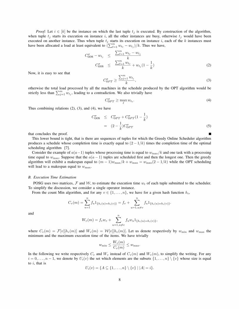
Fig. 4. Average per tuple completion time L with different frequency probability distributions

build these associations using other distributions, namely geometric and binomial, without noticing unpredictabledifferences with respect to the results reported in this section.

We retrieved a dataset containing a stream of preprocessed tweets related to Italian politicians crawled duringthe 2014 European elections. Among other information, the tweets are enriched with a field mention containingthe entities mentioned in the tweet. These entities can be easily classified into politicians, media and others. Weconsider the first 500, 000 tweets, mentioning roughly n = 35, 000 distinct entities and where the most frequententity (“Beppe Grillo”) has an empirical probability of occurrence equal to 0.065.

Evaluation Metrics — The evaluation metrics we provide are (i) the average per tuple completion time: Lalg

(simply average completion time in the following), where alg is the algorithm used for scheduling, and (ii) theaverage per tuple completion time speed up (simply speed up in the following) achieved by POSG with respectto Round-Robin: SL. Recall that lalg(i) is the completion time of the i-th tuple of the stream when using thescheduling algorithm alg. Then we can define the average completion time L

algand speed up SL as follows:

Lalg

=

∑i∈[m] l

alg(i)

mand SL =

∑i∈[m] l

Round-Robin(i)∑i∈[m] l

POSG(i)

Whenever applicable we provide the maximum, mean and minimum figures over the 100 executions.

B. Simulation Results

Frequency Probability Distribution — Figure 4 shows the average completion time L for POSG, Round-Robinand Full Knowledge with different frequency probability distributions. The Full Knowledge algorithm represents anideal execution of the Online Greedy Scheduling algorithm when fed with the exact execution time for each tuple.Increasing the skewness of the distribution reduces the number of distinct tuples that, with high probability, will befed for scheduling, thus simplifying the scheduling process. This is why all algorithms perform better with highlyskewed distributions. On the other hand, uniform or lightly skewed (i.e., Zipf-0.5) distributions seem to be worstcases, in particular for POSG and Round-Robin. With all distributions the Full Knowledge algorithm outperformsPOSG which, in turn, always provide better performance than Round-Robin. However, for uniform or lightly skeweddistributions (i.e., Zipf-0.5), the gain introduced by POSG is limited (in average 6%). Starting with Zipf-1.0 thegain is much more sizeable (25%) and with Zipf-1.5 we have that the maximum average completion time of POSGis smaller than the minimum average completion time of Round-Robin. Finally, with Zipf-2.5 POSG matches theperformance of Full Knowledge. This behavior for POSG stems from the ability of its sketch data structures (Fand W matrices, see Section III) to capture more useful information for skewed input distributions.

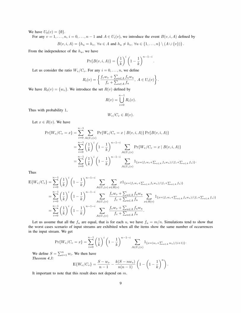
Input Throughput — Figure 5 shows the speed up SL as a function of the percentage of over-provisioning. Whenthe system is strongly undersized (95% to 98%), queuing delays increase sharply, reducing the advantages offeredby POSG. Conversely, when the system is oversized (107 to 115%), queuing delays tend to 0, which in turns alsoreduces the improvement brought by our algorithm. However, in a correctly sized system (i.e., from 100% to 109%),our algorithm introduces a noticeable speed up, in average at least 1.15 with a peak of 1.26 at 102%. Finally, evenwhen the system is largely oversized (115%), we still provide an average speed up of 1.07.

11

0.6

0.8

1

1.2

1.4

1.6

1.8

2

95% 100% 105% 110% 115%

com

plet

ion

time

spee

dup

percentage of overprovisioning

POSG

Fig. 5. Speed up SL as a function of the percentage of over-provisioning

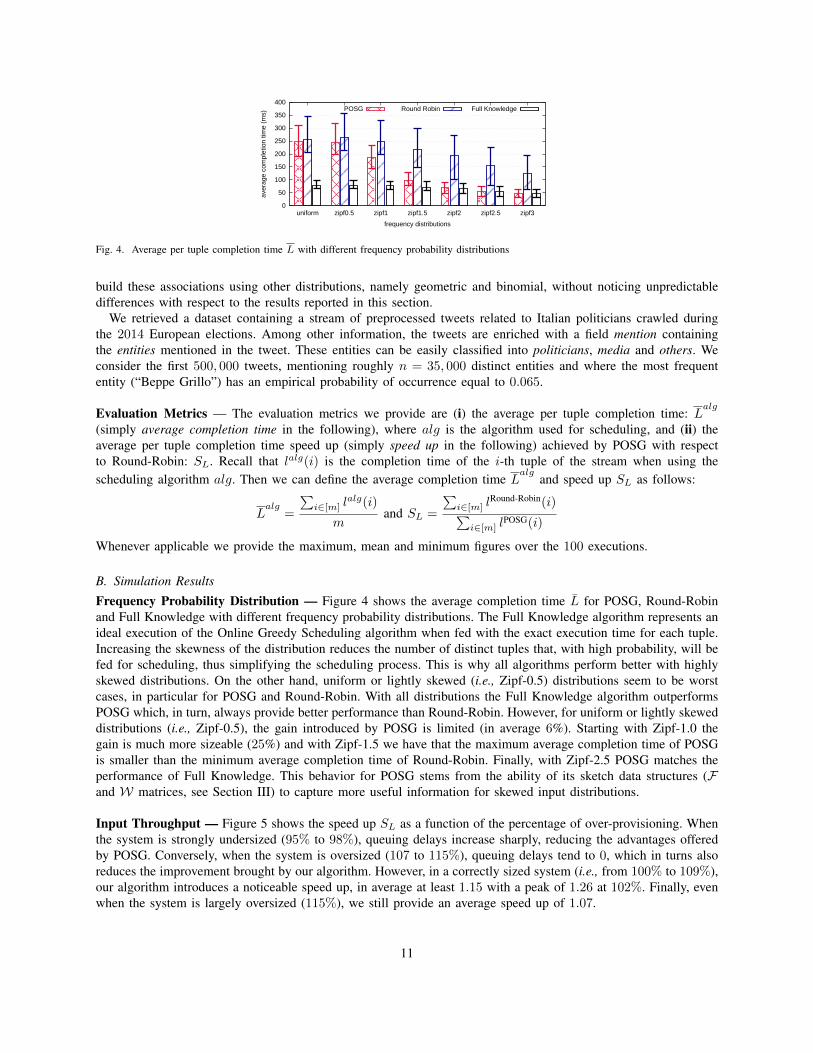
Maximum Execution Time Value — Figure 6 shows the average completion time L as a function of the maximumexecution time wmax. As expected, the average completion time increases with wmax. On the other hand, and quiteunexpectedly, the gain between the maximum, mean and minimum average completion times of POSG with respectto Round-Robin only slightly improves for growing values of wmax, with an average speed up SL of 1.19.

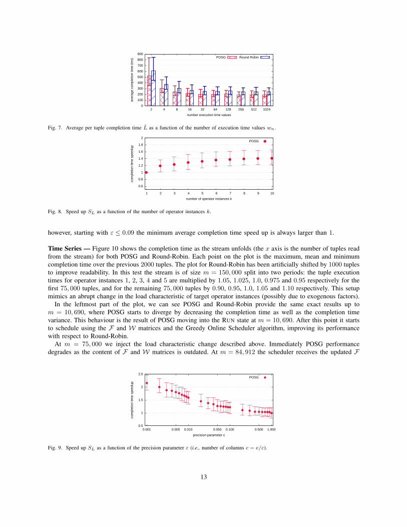
Number of Execution Time Values — Figure 7 shows the average completion time L as a function of the numberof execution time values wn. We can notice that for growing values of wn both the average completion time valuesand variance decrease, with only slight changes for wn ≥ 16. Recall that wn is the number of completion timevalues in the interval [wmin, wmax] that we assign to the n distinct attribute values. For instance, with wn = 2,all the tuples have a completion time equal to either 1 or 64 ms. Then, assigning either of the two values to themost frequent item strongly affects the average completion time. Increasing wn reduces the impact that each singleexecution time has on the average completion time, leading to more stable results. As in the previous plot, thegain between the maximum, mean and maximum average completion times of POSG and Round-Robin (in average19%) is mostly unaffected by the value of wn.

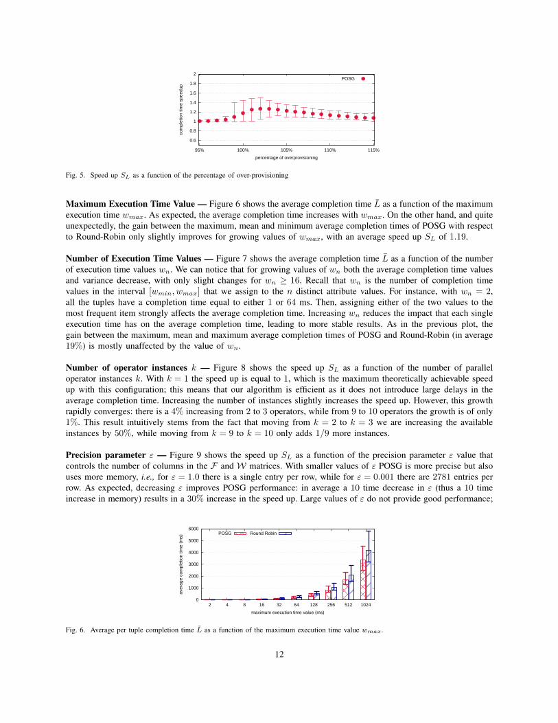
Number of operator instances k — Figure 8 shows the speed up SL as a function of the number of paralleloperator instances k. With k = 1 the speed up is equal to 1, which is the maximum theoretically achievable speedup with this configuration; this means that our algorithm is efficient as it does not introduce large delays in theaverage completion time. Increasing the number of instances slightly increases the speed up. However, this growthrapidly converges: there is a 4% increasing from 2 to 3 operators, while from 9 to 10 operators the growth is of only1%. This result intuitively stems from the fact that moving from k = 2 to k = 3 we are increasing the availableinstances by 50%, while moving from k = 9 to k = 10 only adds 1/9 more instances.

Precision parameter ε — Figure 9 shows the speed up SL as a function of the precision parameter ε value thatcontrols the number of columns in the F and W matrices. With smaller values of ε POSG is more precise but alsouses more memory, i.e., for ε = 1.0 there is a single entry per row, while for ε = 0.001 there are 2781 entries perrow. As expected, decreasing ε improves POSG performance: in average a 10 time decrease in ε (thus a 10 timeincrease in memory) results in a 30% increase in the speed up. Large values of ε do not provide good performance;

0

1000

2000

3000

4000

5000

6000

2 4 8 16 32 64 128 256 512 1024

aver

age

com

plet

ion

time

(ms)

maximum execution time value (ms)

POSG Round Robin

Fig. 6. Average per tuple completion time L as a function of the maximum execution time value wmax.

12

0

100

200

300

400

500

600

700

800

900

2 4 8 16 32 64 128 256 512 1024

aver

age

com

plet

ion

time

(ms)

number execution time values

POSG Round Robin

Fig. 7. Average per tuple completion time L as a function of the number of execution time values wn.

0.6

0.8

1

1.2

1.4

1.6

1.8

2

1 2 3 4 5 6 7 8 9 10

com

plet

ion

time

spee

dup

number of operator instances k

POSG

Fig. 8. Speed up SL as a function of the number of operator instances k.

however, starting with ε ≤ 0.09 the minimum average completion time speed up is always larger than 1.

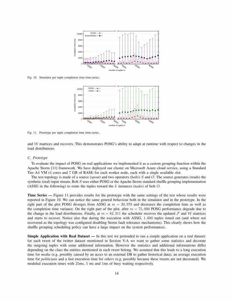
Time Series — Figure 10 shows the completion time as the stream unfolds (the x axis is the number of tuples readfrom the stream) for both POSG and Round-Robin. Each point on the plot is the maximum, mean and minimumcompletion time over the previous 2000 tuples. The plot for Round-Robin has been artificially shifted by 1000 tuplesto improve readability. In this test the stream is of size m = 150, 000 split into two periods: the tuple executiontimes for operator instances 1, 2, 3, 4 and 5 are multiplied by 1.05, 1.025, 1.0, 0.975 and 0.95 respectively for thefirst 75, 000 tuples, and for the remaining 75, 000 tuples by 0.90, 0.95, 1.0, 1.05 and 1.10 respectively. This setupmimics an abrupt change in the load characteristic of target operator instances (possibly due to exogenous factors).

In the leftmost part of the plot, we can see POSG and Round-Robin provide the same exact results up tom = 10, 690, where POSG starts to diverge by decreasing the completion time as well as the completion timevariance. This behaviour is the result of POSG moving into the RUN state at m = 10, 690. After this point it startsto schedule using the F and W matrices and the Greedy Online Scheduler algorithm, improving its performancewith respect to Round-Robin.

At m = 75, 000 we inject the load characteristic change described above. Immediately POSG performancedegrades as the content of F and W matrices is outdated. At m = 84, 912 the scheduler receives the updated F

0.5

1

1.5

2

2.5

0.001 0.005 0.010 0.050 0.100 0.500 1.000

com

plet

ion

time

spee

dup

precision parameter ε

POSG

Fig. 9. Speed up SL as a function of the precision parameter ε (i.e., number of columns c = e/ε).

13

0

2000

4000

6000

8000

10000

10000 20000

30000

com

plet

ion

time

(ms)

POSGRound Robin

70000 80000

90000

number of tuples m

Fig. 10. Simulator per tuple completion time time-series.

0

2000

4000

6000

8000

10000

10000 20000

30000

com

plet

ion

time

(ms)

POSGASSG

70000 80000

90000

number of tuples m

Fig. 11. Prototype per tuple completion time time-series.

and W matrices and recovers. This demonstrates POSG’s ability to adapt at runtime with respect to changes in theload distributions.

C. Prototype

To evaluate the impact of POSG on real applications we implemented it as a custom grouping function within theApache Storm [11] framework. We have deployed our cluster on Microsoft Azure cloud service, using a StandardTier A4 VM (4 cores and 7 GB of RAM) for each worker node, each with a single available slot.

The test topology is made of a source (spout) and two operators (bolts) S and O. The source generates (reads) thesynthetic (real) input stream. Bolt S uses either POSG or the Apache Storm standard shuffle grouping implementation(ASSG in the following) to route the tuples toward the k instances (tasks) of bolt O.

Time Series — Figure 11 provides results for the prototype with the same settings of the test whose results werereported in Figure 10. We can notice the same general behaviour both in the simulator and in the prototype. In theright part of the plot POSG diverges from ASSG at m = 20, 978 and decreases the completion time as well asthe completion time variance. On the right part of the plot, after m = 75, 000 POSG performance degrade due tothe change in the load distributions. Finally, at m = 82, 311 the scheduler receives the updated F and W matricesand starts to recover. Notice also that during the execution with ASSG, 1, 600 tuples timed out (and where notrecovered as the topology was configured disabling Storm fault tolerance mechanisms). This clearly shows how theshuffle grouping scheduling policy can have a large impact on the system performances.

Simple Application with Real Dataset — In this test we pretended to run a simple application on a real dataset:for each tweet of the twitter dataset mentioned in Section V-A we want to gather some statistics and decoratethe outgoing tuples with some additional information. However the statistics and additional informations differdepending on the class the entities mentioned in each tweet belong. We assumed that this leads to a long executiontime for media (e.g. possibly caused by an acces to an external DB to gather historical data), an average executiontime for politicians and a fast execution time for others (e.g. possibly because these tweets are not decorated). Wemodeled execution times with 25ms, 5 ms and 1ms of busy waiting respectively.

14

10

20

30

40

50

60

70

80

90

100

110

01 02 03 04 05 06 07 08 09 10

aver

age

com

plet

ion

time

(ms)

number of operator instances k

POSG ASSG

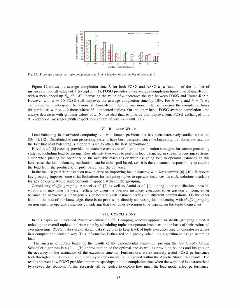
Fig. 12. Prototype average per tuple completion time L as a function of the number of operators k.

Figure 12 shows the average completion time L for both POSG and ASSG as a function of the number ofinstances k. For all values of k (except k = 1), POSG provides lower average completion times than Round-Robin,with a mean speed up SL of 1.37. Increasing the value of k decreases the gap between POSG and Round-Robin.However with k = 10 POSG still improves the average completion time by 16%. For k = 2 and k = 7, wecan notice an unanticipated behaviour of Round-Robin: adding one more instance increases the completion times(in particular, with k = 2 there where 221 timeouted tuples). On the other hand, POSG average completion timealways decreases with growing values of k. Notice also that, to provide this improvement, POSG exchanged only916 additional messages (with respect to a stream of size m = 500, 000).

VI. RELATED WORK

Load balancing in distributed computing is a well known problem that has been extensively studied since the80s [3], [12]. Distributed stream processing systems have been designed, since the beginning, by taking into accountthe fact that load balancing is a critical issue to attain the best performance.

Hirzel et al. [8] recently provided an extensive overview of possible optimization strategies for stream processingsystems, including load balancing. They identify two ways to perform load balancing in stream processing systems:either when placing the operators on the available machines or when assigning load to operator instances. In thislatter case, the load balancing mechanism can be either pull based, i.e., it is the consumers responsibility to acquirethe load from the producers, or push based, i.e., the converse.

In the the last year there has been new interest on improving load balancing with key grouping [6], [10]. However,key grouping imposes some strict limitations for assigning tuples to operator instances; as such, solutions availablefor key grouping would underperform if applied with shuffle grouping.

Considering shuffle grouping, Arapaci et al. [2] as well as Amini et al. [1], among other contributions, providesolutions to maximise the system efficiency when the operator instances execution times are non uniform, eitherbecause the hardware is etherogeneous or because each instance carries out different computations. On the otherhand, at the best of our knowledge, there is no prior work directly addressing load balancing with shuffle groupingon non uniform operator instances considering that the tuples execution time depend on the tuple themselves.

VII. CONCLUSIONS

In this paper we introduced Proactive Online Shuffle Grouping, a novel approach to shuffle grouping aimed atreducing the overall tuple completion time by scheduling tuples on operator instances on the basis of their estimatedexecution time. POSG makes use of sketch data structures to keep track of tuple execution time on operator instancesin a compact and scalable way. This information is then fed to a greedy scheduling algorithm to assign incomingload.

The analysis of POSG backs up the results of the experimental evaluation, proving that the Greedy OnlineScheduler algorithm is a (2− 1/k)-approximation of the optimal one as well as providing bounds and insights onthe accuracy of the estimation of the execution time wt. Furthermore, we extensively tested POSG performanceboth through simulations and with a prototype implementation integrated within the Apache Storm framework. Theresults showed how POSG provides important speedups in tuple completion time when the workload is characterizedby skewed distributions. Further research will be needed to explore how much the load model affect performance.

15

For example it would be interesting to include other metrics in the load model, e.g. network latencies, to checkhow much these may improve the overal performance.

REFERENCES

[1] L. Amini, N. Jain, A. Sehgal, J. Silber, and O. Verscheure. Adaptive control of extreme-scale stream processing systems. In Proceedingsof the 26th IEEE International Conference on Distributed Computing Systems, ICDCS, 2006.

[2] R. H. Arpaci-Dusseau, E. Anderson, N. Treuhaft, D. E. Culler, J. M. Hellerstein, D. Patterson, and K. Yelick. Cluster i/o with river:Making the fast case common. In Proceedings of the 6th Workshop on Input/Output in Parallel and Distributed Systems, IOPADS, 1999.

[3] V. Cardellini, E. Casalicchio, M. Colajanni, and P. S. Yu. The state of the art in locally distributed web-server systems. ACM ComputingSurveys, 34(2), 2002.

[4] J. L. Carter and M. N. Wegman. Universal classes of hash functions. Journal of Computer and System Sciences, 18, 1979.[5] G. Cormode and S. Muthukrishnan. An improved data stream summary: The count-min sketch and its applications. Journal of Algorithms,

55, 2005.[6] B. Gedik. Partitioning functions for stateful data parallelism in stream processing. The VLDB Journal, 23(4), 2014.[7] D. Gusfield. Bound the naive multiple machine scheduling with release times deadlines. Journal of Algorithms, (5):1–6, 1984.[8] M. Hirzel, R. Soule, S. Schneider, B. Gedik, and R. Grimm. A catalog of stream processing optimizations. ACM Comput. Surv., 46(4),

2014.[9] Muthukrishnan. Data Streams: Algorithms and Applications. Now Publishers Inc., 2005.

[10] N. Rivetti, L. Querzoni, E. Anceaume, Y. Busnel, and B. Sericola. Efficient key grouping for near-optimal load balancing in streamprocessing systems. In Proceedings of the 9th ACM International Conference on Distributed Event-Based Systems, DEBS, 2015.

[11] The Apache Software Foundation. Apache Storm. http://storm.apache.org.[12] S. Zhou. Performance Studies of Dynamic Load Balancing in Distributed Systems. PhD thesis, UC Berkeley, 1987.

16