probabilistic fatigue design of shaft for bending and torsion

IJRET: International Journal of Research in Engineering and Technology eISSN: 2319-1163 | pISSN: 2321-7308

_______________________________________________________________________________________

Volume: 03 Issue: 09 | Sep-2014, Available @ http://www.ijret.org 370

PROBABILISTIC FATIGUE DESIGN OF SHAFT FOR BENDING AND

TORSION

Osakue, E. Edward1

1Texas Southern University, Houston, Texas, USA

Abstract The ever increasing demand for better and reliable mechanical systems necessitates the explicit consideration of reliability in the

modeling and design of these systems. Design for reliability (DFR) has been receiving a great deal of attention for several years

and companies are deploying resources to the design for reliability process because of the need to satisfy customers and reduce

warranty costs. In traditional or deterministic design, safety or design factors are usually subjectively assigned in product design

so as to assure reliability. But this method of design does not provide a logical basis for addressing uncertainties, so the level of

reliability cannot be assessed quantitatively.

This paper presents a probabilistic design approach for shafts under combined bending and torsional loads using the generalized

Gerber fatigue failure rule. The design model parameters are considered as random variables characterized by mean values and

coefficients of variation (covs). The coefficient of variation of the shaft design model is obtained by using first order Taylor series

expansion for strength and stress in a stress-life fatigue design. A reliability factor is defined and related to the covs of design

parameters and a failure probability. The design model assumes a lognormal probability density distribution for the parameters.

This approach thus accounts for variability of design model parameters and provides quantitative assessment of product

reliability. The approach is flow-charted for ease of application.

This study shows that deterministic engineering models can be transformed into probabilistic models that can predict the risk in a

design situation. From the design examples considered, it is shown that the popular modified Goodman model (MGM) for stress-

life fatigue design is slightly on the conservative side. The study indicates possible reduction in component size and hence savings

in product cost can be obtained through probabilistic design. Probabilistic design seems to be the most practical approach in

product design due to the inherent variability associated with service loads, material properties, geometrical attributes, and

mathematical design models. The computations in the present model were done using Microsoft Excel. This demonstrates that

probabilistic design can be simplified so that specialized software and skills may not be required, especially at the preliminary

design phase. Very often, available probabilistic models are intensive in numerical computation, requiring custom software and

skilled personnel. The model approach presented needs to be explored for other design applications, so as to the make

probabilistic design a common practice.

Keywords: Fatigue, Failure, Reliability, Lognormal, Safety

-------------------------------------------------------------------***-------------------------------------------------------------------

1. INTRODUCTION

When a consumer buys a product, he or she expects it to

function at least to the advertised performance standard(s) or

specification(s) of the seller or manufacturer. In addition,

there is the implied expectation of reliability and safety, for

no customer would knowingly buy a product that is

unreliable or worst still, unsafe! A good engineering design

requires considering functionality, reliability, safety,

manufacturability, operability, maintainability, and

affordability. According to Hammer [1], a good engineer

designs a product to preclude failures, accidents, injuries,

and damages. Hence safety is at the heart of good

engineering design practice. Designing safe products have

been done for decades, or perhaps centuries, on the basis of

a safety factor, a number greater than unity. A safety factor

is subjectively assigned in practice so this approach does not

provide a logical basis for addressing uncertainties or

variability. With the safety factor method, the level of

reliability cannot be assessed quantitatively [2], hence the

safety margin in a design is practically unknown. Because of

the difficulty of relating safety factor and product safety

quantitatively, some prefer the term “design factor” to

“safety factor” [3]. It is desirable to design components and

products to expected levels of reliability (or failure

probability), with the target level of reliability depending on

specific consequences of failure. This would allow the

development of risk-informed design methods and may

result in potential savings [4].

A quantitative assessment of reliability, and hence safety, is

possible through applications of probability and statistics.

Therefore, statistical-probabilistic or reliability-based design

has attracted great attention in the last few decades. For

instance, Load and Resistance Factored Design (LRFD), a

reliability-based method, has been developed and is being

used in structural design. This approach is being studied for

adoption in piping design. Reliability-based designs promote

consistency, allow more efficient designs, and are more

flexible and rational than working stress or safety factor


_______________________________________________________________________________________


methods because they provide consistent levels of safety

over various types of structures and products [4].

Probabilistic design allows a quantification of risk that can

help to avoid over- or under-design problems while ensuring

that safety and quality levels are economically achieved [5].

Over design requires more resources than necessary and

leads to costly products. Avoiding over-design helps to

conserve product materials and reduce manufacturing

resources, machining accuracy, quality control, etc. during

processing. Under-designed products are prone to failures,

making the products unsafe and unreliable. This increases

the risks of product liability lawsuits, customer

dissatisfaction, and even accidents [6]. Much research has

been done in recent years on quantifying uncertainties in

engineering systems and their effects on reliability.

In most real engineering problems, variation is inherent in

material properties, loading conditions, geometric

properties, simulation models, manufacturing precision,

actual product usage, etc. [4, 7, 8]. Environmental

conditions affect the reliability and service life of products.

Temperature and humidity are probably two of such

conditions that can significantly affect reliability [9]. But

rain, hail, water quality, wind, snow, mud, sand, dust, etc.

can also influence product reliability and service life [9].

Environmental conditions affect both service loads and

material mechanical properties. It is not physically possible

or financially feasible to eliminate variation of geometric

design parameters. This is due to the fact that the reduction

of variability is associated with higher costs either through

better and more precise manufacturing methods and

processes or increased efforts in quality. Accepting

variability and limiting it is a more practical approach in

design as it makes production more cost-effective and

products more affordable [10]. In general, variability in

stress-based design parameters can be grouped into two:

strength variability and stress variability. Stress variability

has two components of load variability and geometric

variability. Generally, the variability of geometry is usually

of a lesser degree compared to the variability in material

properties or loads.

As mentioned earlier, a component or product failure

probability should reflect the consequence of failure such as

product damage or personnel injury [11, 12, 13]. According

to Socie [14], failure probability of 10-6

to 10-9

for safety and

10-2

to 10-4

for economic damage may be considered

acceptable. The aerospace industry specifies a failure

probability of 10-5

in many cases, while the standard failure

probability of rolling element bearings is 10-1

[11]. Ashby

and Jones [15] says a failure probability of 10-1

may be

acceptable for ceramic tool because it is easily replaced but

one may aim at a value of 10-6

where failure may result in

injury and probably 10-8

when one component failure could

be fatal.

The use of probabilistic design methods requires some

appropriate probability distribution [16]. The lognormal

probability distribution has inherent properties that

recommend it for machine and structural design applications

[17, 18]. Therefore, it is assumed in this study that the

strengths of materials and service loads on equipment are

distributed in the standard lognormal sense. Agrawal [19]

observed that the cross-sectional area of structural members

depended on the mean strength and standard deviation

values of materials for a given load distribution [19]. This

suggests that the coefficient of variation (cov), the ratio of

standard deviation to mean value of model parameters, is

appropriate for probabilistic design. The use of the cov is

particularly desirable since it can be used to summarize the

variability of a group of materials and equipment in an

industrial sector [20, 21]. As will be seen later, the cov fits

in easily in the lognormal probability model.

The most problematic design situation is dynamic where

machine and structural members are subjected to fatigue

loading. About 80% to 90% of the failures of machine and

structural members result from fatigue [22, 23]. Fatigue

failure normally takes the form of brittle fracture at stresses

well below the static strength of the materials [3, 24] which

can be catastrophic sometimes. Fatigue failures are more

likely when a tensile mean stress is present during a fatigue

load cycle. Several models [11, 25] are available in literature

addressing the influence of tensile mean stress on fatigue

life. Among these are the Gerber (Germany, 1874),

Goodman (England, 1899), and Soderberg (USA, 1930).

According to Norton [25], the Gerber parabola fits

experimental data on fatigue failure with reasonable

accuracy, though considerable scatter exists. He noted that

the Gerber parabola is a measure of the average behavior of

ductile materials in fatigue resistance while the modified

Goodman curve is that of minimum behavior. Shingley and

Mischke [17], state that the Gerber parabola falls centrally

on experimental data while the modified Goodman line does

not. The modified Goodman criterion is in common but the

Solderberg model is rarely used now because it is very

conservative.

Because the traditional Gerber bending fatigue criterion

captures fatigue failure data on an average performance

basis; it can be associated with 50% reliability [18]. The

model is therefore a strong candidate for probabilistic design

if mean values of design parameters are used in it. Higher or

lower reliabilities can be achieved through specific failure

probability requirement and variability of design model

parameters. Direct reliability-based design requires

performing spectral analysis and extreme value analysis of

loads. Serviceability and failure modes needs to be

considered at different levels and appropriate loads, strength

capacities, failure definitions need to be selected for each

failure mode [4]. Now, several reliability-based design

approaches have been proposed in the last five decades [2].

However, they are generally computationally intensive,

involve numerical modeling, require specialized software, or

require specialized skills. These seem to have restricted their

use to complex and costly design applications. Mischke [26]

stated that deterministic and familiar engineering

computations are useful in stochastic problems if mean

values are used. Therefore, deterministic models are suitable

for probabilistic design if the variability of design model


_______________________________________________________________________________________


parameters is accounted for. Such an approach may simplify

probabilistic design and alleviate issues of using

complicated models and encourage the use of probabilistic

design in conceptual and preliminary phases in a design

project. Excel based design software can lead to reduction in

design cost, and also speed up design as preliminary model

sizes will be more accurate [27, 28].

2. LOGNORMAL RELIABILITY MODEL

The lognormal probability distribution function has inherent

properties that make it an attractive choice for engineering

design applications. For instance, the products and quotients

of lognormal variates are lognormal and real powers of

lognormal variates are also lognormal [17]. Now most

design formulas are products and sums of design

parameters: so they can be assumed to have lognormal

distribution as a first approximation. Suppose in a strength-

stress design model and in the physical domain, S andrepresent strength and stress, respectively. S is the random

variable for strength with mean value of s , standard

deviation of s , and cov of s . is the random variable

for stress with mean value of , standard deviation of ,

and cov of . Then:

s

ss

1

A random variable n with parameters nn and μ can be

defined as the ratio of S and σ. That is:

Sn 2a

22 sn 2b

To preclude failure, n must be greater than unity: that is,

S If S , then failure has occurred. Since S and

have lognormal distributions, respectively, the quotient

,n will be lognormal in distribution [17]. If q is the random

variable for the quotient n in the lognormal domain, then:

Snq ln)(ln

3

Based on the properties of lognormal distribution [29], if the

parameters of q are q and q , then:

25.0ln qnq 4a

21ln nq 221ln s 4b

The probability density distribution of q is normal and is

depicted in Fig. 1a. Fig. 1b depicts the corresponding unit

normal variate distribution. The failure probability

associated with the unit normal variate is represented by the

area under the normal distribution curve (shaded in Fig. 1b)

and corresponds to the failure region in Fig. 1a (shaded).

a). Normal distribution

b) Unit normal distribution

Fig. 1: Random variable with normal distribution

The failure zone of a component or product is the region of

0q where 1n . Referring to Fig. 1b, any normal

variate q on the left of q in Fig. 1a corresponding to -z on

the left of the origin in Fig. 1b can be obtained as:

qq zq 5

Hence when 0q :

q

qz

22

22

1ln

1ln5.0)(ln

efs

efsn

6

In a stress-strength based design, the reliability factor may

be defined as:

ef

Szn

Stress EffectiveMean

Capabilty StressMean 7

qµq

Failure

region

0

-z z0

Failure

region


_______________________________________________________________________________________


In fatigue design, fS S or utS S in Eqn. 7, depending

on the most likely failure mode [30]. For design application,

it may be assumed that zn n [17] in Equation (6). An

engineering model can be deduced from Eqns. 4a and 4b by

introducing a slight modification on q

expression by

changing it to the value predicted by strength-stress overlap

in probability density functions. This is given by [17, 18]:

)1)(1(ln 22efsq )1(ln 2222

efsefs

8

Notice the product term (22efs ) in Eqn. 8 which is absent

from Eqn. 4b. This implies that the value of q from Eqn. 8

will be slightly higher than that from Eqn. 4b. If Eqn. 8 is

substituted in Eqn. 6; we have:

)1)(1(ln

)1)(1(ln5.0)(ln

22

22

efs

efsznz

9

Eqn. 9 gives the unit normal variate z , based on the

reliability factor and design model parameters variability.

The substitution of Eqn. 8 for Eqn. 4b in Eqn. 6 to obtain

Eqn. 9; slightly increases the denominator and

simultaneously decreases the numerator. The overall effect

of this is the reduction of the unit normal variate or z-

variable, so that the predicted reliability is conservative.

This reliability is obtained as:

)()(1 zzRz ` 10

Eqn. 10 gives the reliability for the unit normal variate ,z

with the value of )( z or )(z read from an appropriate

table. If a desired reliability or failure probability is

specified then, z is known and the necessary reliability

factor zn for achieving this reliability level can be obtained.

That is from Eqn. 9:

)1)(1(ln5.0

)1)(1(lnexp

22

22

efs

efs

z

zn

11

From Eqn. 11, if the variability of the significant factors in a

design model can be estimated with reasonable accuracy, it

is possible to design to a reliability target through a

reliability factor. According to Wang, Kim and Kim [31], it

is common to use the unit normal variate (Eqn. 9) for failure

probability assessment because probability values (Eqn. 10)

can change by several orders of magnitude over small

changes in the unit normal variate. Since small changes in z

could mean relatively higher changes in zR ; Eqn. 9 should

yield conservative results for zR and perhaps allows its use in

high reliability situations. An alternative to reading zR from

Tables is discussed in the Appendix.

The mean and standard deviation or cov of design models

must be evaluated in order to apply Eqns. 9, 10, and 11.

Suppose a function χ, has the random variables

nxxxx .......,, 321as independent variables. Then:

).......,,( 321 nxxxxf 12

Based on Taylor series expected values for unskewed or

lightly skewed distributions [17], a first order estimate of the

mean and standard deviation of χ may be obtained

respectively:

).......,,( 321 xnxxxf 13a

2

2

1ix

n

i ix

13b

The coefficient of variation is the ratio of standard deviation

to the mean value:

14

Eqn. 13a simply says that the mean value of a function is

obtained by substituting mean values of its independent

variables. Eqns. 13b and 14 provide means of quickly

obtaining the standard deviation and cov of the function

using partial differentiation. The task in using the reliability

model of Eqn. 9 is to develop expressions for S and ef

for specific design models. Eqns.13a, 13b, and 14 are

helpful in this task. The model application is not limited to

stress-based design; it can be used for any serviceability

criterion of interest such as lateral stability, transverse

deflection, torsional rigidity, critical speed, etc. In this

study, expressions for S and ef for Gerber bending

fatigue failure rule for combined bending and torsional loads

are developed.

3. FATIGUE DESIGN

A component or product is loaded in fatigue if it is subjected

to some repeated force or bending moment loads. A load

cycle is when the imposed load changes value from a

minimum to a maximum and back to the minimum. Fatigue

load cycles may be classified into two groups of finite-life

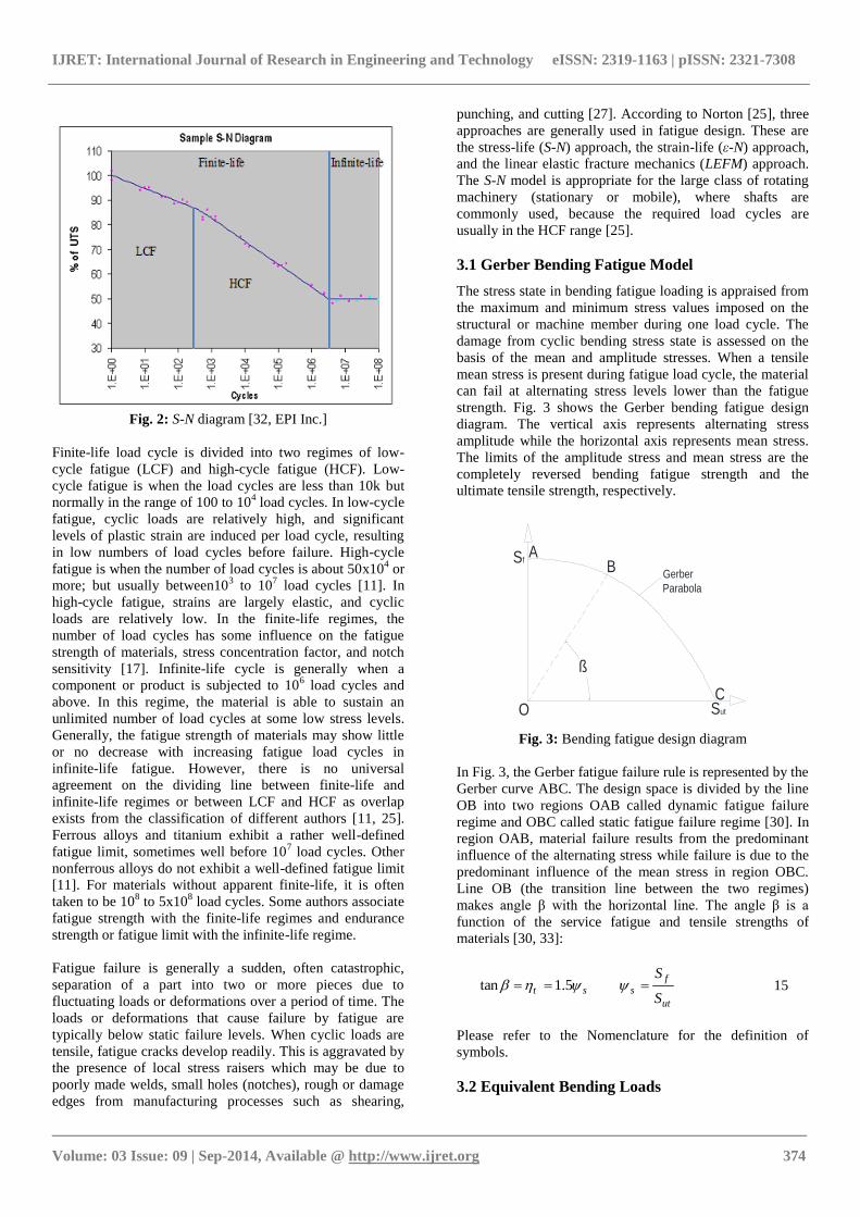
and infinite-life load cycles as shown in Fig. 2, which is

called the S-N diagram. The vertical axis represents stress

while the horizontal axis represents load cycles. In finite-life

load cycle, a component or product fails at a limited number

of load cycles and the life of the component is measured as

the number of load cycles to failure.


_______________________________________________________________________________________


Fig. 2: S-N diagram [32, EPI Inc.]

Finite-life load cycle is divided into two regimes of low-

cycle fatigue (LCF) and high-cycle fatigue (HCF). Low-

cycle fatigue is when the load cycles are less than 10k but

normally in the range of 100 to 104 load cycles. In low-cycle

fatigue, cyclic loads are relatively high, and significant

levels of plastic strain are induced per load cycle, resulting

in low numbers of load cycles before failure. High-cycle

fatigue is when the number of load cycles is about 50x104 or

more; but usually between103 to 10

7 load cycles [11]. In

high-cycle fatigue, strains are largely elastic, and cyclic

loads are relatively low. In the finite-life regimes, the

number of load cycles has some influence on the fatigue

strength of materials, stress concentration factor, and notch

sensitivity [17]. Infinite-life cycle is generally when a

component or product is subjected to 106 load cycles and

above. In this regime, the material is able to sustain an

unlimited number of load cycles at some low stress levels.

Generally, the fatigue strength of materials may show little

or no decrease with increasing fatigue load cycles in

infinite-life fatigue. However, there is no universal

agreement on the dividing line between finite-life and

infinite-life regimes or between LCF and HCF as overlap

exists from the classification of different authors [11, 25].

Ferrous alloys and titanium exhibit a rather well-defined

fatigue limit, sometimes well before 107 load cycles. Other

nonferrous alloys do not exhibit a well-defined fatigue limit

[11]. For materials without apparent finite-life, it is often

taken to be 108 to 5x10

8 load cycles. Some authors associate

fatigue strength with the finite-life regimes and endurance

strength or fatigue limit with the infinite-life regime.

Fatigue failure is generally a sudden, often catastrophic,

separation of a part into two or more pieces due to

fluctuating loads or deformations over a period of time. The

loads or deformations that cause failure by fatigue are

typically below static failure levels. When cyclic loads are

tensile, fatigue cracks develop readily. This is aggravated by

the presence of local stress raisers which may be due to

poorly made welds, small holes (notches), rough or damage

edges from manufacturing processes such as shearing,

punching, and cutting [27]. According to Norton [25], three

approaches are generally used in fatigue design. These are

the stress-life (S-N) approach, the strain-life (ε-N) approach,

and the linear elastic fracture mechanics (LEFM) approach.

The S-N model is appropriate for the large class of rotating

machinery (stationary or mobile), where shafts are

commonly used, because the required load cycles are

usually in the HCF range [25].

3.1 Gerber Bending Fatigue Model

The stress state in bending fatigue loading is appraised from

the maximum and minimum stress values imposed on the

structural or machine member during one load cycle. The

damage from cyclic bending stress state is assessed on the

basis of the mean and amplitude stresses. When a tensile

mean stress is present during fatigue load cycle, the material

can fail at alternating stress levels lower than the fatigue

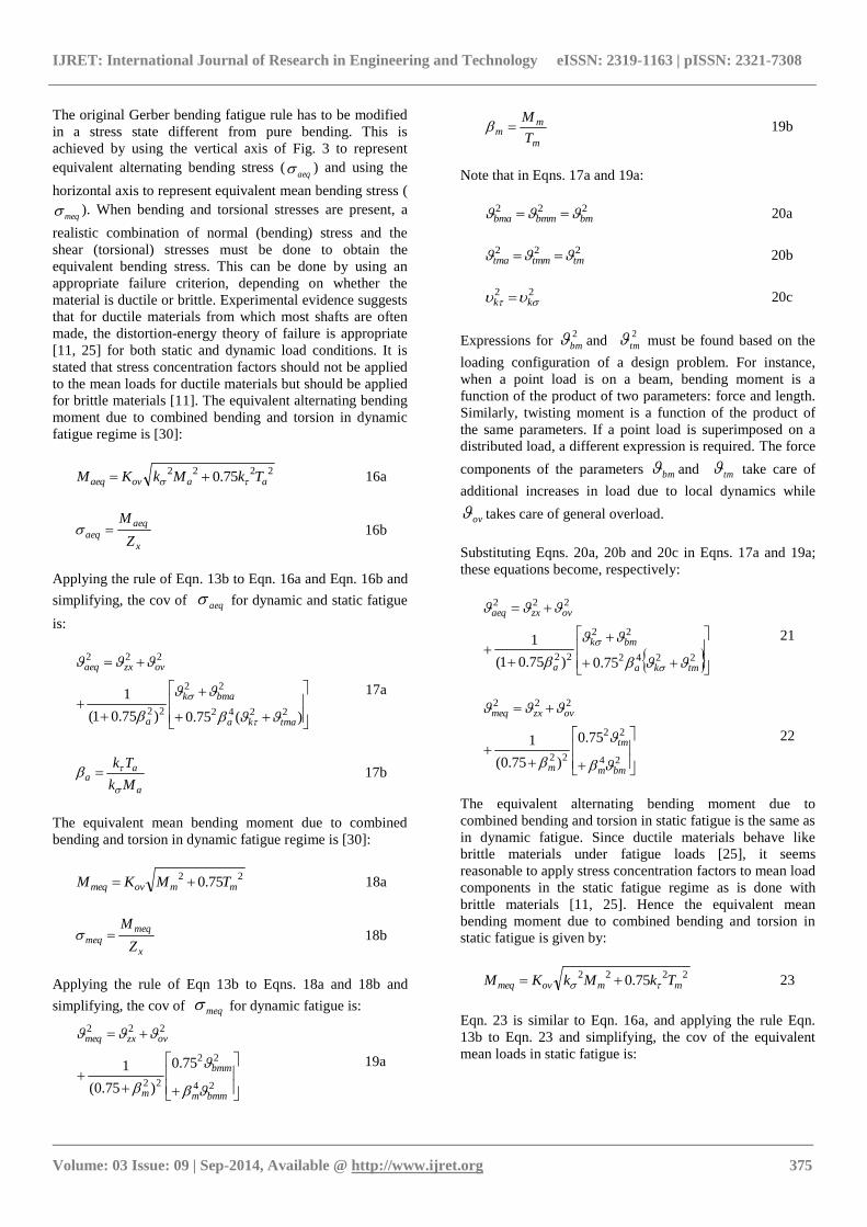
strength. Fig. 3 shows the Gerber bending fatigue design

diagram. The vertical axis represents alternating stress

amplitude while the horizontal axis represents mean stress.

The limits of the amplitude stress and mean stress are the

completely reversed bending fatigue strength and the

ultimate tensile strength, respectively.

Fig. 3: Bending fatigue design diagram

In Fig. 3, the Gerber fatigue failure rule is represented by the

Gerber curve ABC. The design space is divided by the line

OB into two regions OAB called dynamic fatigue failure

regime and OBC called static fatigue failure regime [30]. In

region OAB, material failure results from the predominant

influence of the alternating stress while failure is due to the

predominant influence of the mean stress in region OBC.

Line OB (the transition line between the two regimes)

makes angle β with the horizontal line. The angle β is a

function of the service fatigue and tensile strengths of

materials [30, 33]:

ut

f

sstS

S 5.1tan 15

Please refer to the Nomenclature for the definition of

symbols.

3.2 Equivalent Bending Loads

SfB

A

Sut

CO

ß

Gerber

Parabola


_______________________________________________________________________________________


The original Gerber bending fatigue rule has to be modified

in a stress state different from pure bending. This is

achieved by using the vertical axis of Fig. 3 to represent

equivalent alternating bending stress (aeq ) and using the

horizontal axis to represent equivalent mean bending stress (

meq ). When bending and torsional stresses are present, a

realistic combination of normal (bending) stress and the

shear (torsional) stresses must be done to obtain the

equivalent bending stress. This can be done by using an

appropriate failure criterion, depending on whether the

material is ductile or brittle. Experimental evidence suggests

that for ductile materials from which most shafts are often

made, the distortion-energy theory of failure is appropriate

[11, 25] for both static and dynamic load conditions. It is

stated that stress concentration factors should not be applied

to the mean loads for ductile materials but should be applied

for brittle materials [11]. The equivalent alternating bending

moment due to combined bending and torsion in dynamic

fatigue regime is [30]:

222275.0 aaovaeq TkMkKM 16a

x

aeqaeq

Z

M 16b

Applying the rule of Eqn. 13b to Eqn. 16a and Eqn. 16b and

simplifying, the cov of aeq for dynamic and static fatigue

is:

)(75.0)75.01(

12242

22

22

222

tmaka

bmak

a

ovzxaeq

17a

a

aa

Mk

Tk

17b

The equivalent mean bending moment due to combined

bending and torsion in dynamic fatigue regime is [30]:

2275.0 mmovmeq TMKM 18a

x

meqmeq

Z

M 18b

Applying the rule of Eqn 13b to Eqns. 18a and 18b and

simplifying, the cov of meq for dynamic fatigue is:

24

22

22

222

75.0

)75.0(

1

bmmm

bmm

m

ovzxmeq

19a

m

mm

T

M 19b

Note that in Eqns. 17a and 19a:

222bmbmmbma 20a

222tmtmmtma 20b

22 kk 20c

Expressions for 2

bm and 2

tm must be found based on the

loading configuration of a design problem. For instance,

when a point load is on a beam, bending moment is a

function of the product of two parameters: force and length.

Similarly, twisting moment is a function of the product of

the same parameters. If a point load is superimposed on a

distributed load, a different expression is required. The force

components of the parameters bm and tm take care of

additional increases in load due to local dynamics while

ov takes care of general overload.

Substituting Eqns. 20a, 20b and 20c in Eqns. 17a and 19a;

these equations become, respectively:

2242

22

22

222

75.0)75.01(

1

tmka

bmk

a

ovzxaeq

21

24

22

22

222

75.0

)75.0(

1

bmm

tm

m

ovzxmeq

22

The equivalent alternating bending moment due to

combined bending and torsion in static fatigue is the same as

in dynamic fatigue. Since ductile materials behave like

brittle materials under fatigue loads [25], it seems

reasonable to apply stress concentration factors to mean load

components in the static fatigue regime as is done with

brittle materials [11, 25]. Hence the equivalent mean

bending moment due to combined bending and torsion in

static fatigue is given by:

222275.0 mmovmeq TkMkKM 23

Eqn. 23 is similar to Eqn. 16a, and applying the rule Eqn.

13b to Eqn. 23 and simplifying, the cov of the equivalent

mean loads in static fatigue is:


_______________________________________________________________________________________


2244

222

222

222

)(75.0

)75.0(

1

bmkm

tmk

m

ovzxmeq

KK

24a

k

kK

24b

A design point is defined by the coordinates ( ), aeqmeq

which has a load line that passes through the origin with a

slope [30] given by

meq

aeq

meq

aeq

M

M

25

If η is equal to or greater than the load line transition factor

t , then the design point will be inside the region OAB in

Fig. 3 and dynamic fatigue failure applies. If is less than

t ; then the design point will

be inside the region OBC in Figure 3, and static fatigue

failure applies.

3.3 Dynamic Fatigue Failure Regime:t

The design load capability in dynamic fatigue failure is

determined by the service fatigue strength. If direct field

measurements are made, fs is obtained from test results.

However, laboratory fatigue tests on small polished

specimens of the material of interest [11, 17, 25] can be used

to estimate field or service fatigue strength by making use of

adjustment or correction factors. In such a case, the service

fatigue strength (Eqn. 26a) and coefficient of variation of

the fatigue strength (Eqn. 26b) are estimated respectively as:

/

tpsrsz C C C ff SS 26a

2

1

2222tpsrszfbfsS 26b

Alternatively, the basic fatigue strength may be estimated

from the tensile strength and the service fatigue strength

(Eqn. 27a) and coefficient of variation of the fatigue

strength (Eqn. 27b) are estimated respectively as:

/

tpsrsz C C C utof SS 27a

2

122222tpsrszosufsS 27b

In design sizing and for the initial or first time estimate of

shaft size, values of k , k and zn are required. The

problem is that these factors depend on the shaft size which

is yet unknown. For preliminary design, values of k and

k , may be assumed [25] or set equal to /

k and/

k ,

respectively. But /

k is less than k and k is less than/

k

due to the influence of notch sensitivity. For a first time

estimate of size, a design factor on can be used instead of

zn (please refer to the Appendix) whereby on is

approximated from the expression for zn (Eqn. 11). The no

for estimating on is obtained as:

2

12222 )(5.0 mequtaeqmisno 28a

Eqn. 28a is obtained from Eqn. 32 by assuming

mn = 2. Then Eqn. 11 is used to obtain on as:

)1)(1(ln5.0

)1)(1(lnexp

22

22

nos

nosoo

zn

28b

For a solid shaft, the initial size estimate is [30]:

3

1

22

22

75.05.0

75.032

mms

aa

f

oov

TM

TkMk

S

nKd

29

Eqn. 29 is of general application for solid circular shafts

only. It can easily be modified for a hollow shaft. For the

case of fully reversed bending and steady torque; Mm = 0

and Ta = 0 and:

3

1

325.032

msaf

oov TMkS

nKd

30

From [30], ef for generalized Gerber rule in dynamic

fatigue is:

2

11

m

aeq

ef

n

31a

meq

utm

Sn

31b


_______________________________________________________________________________________


From [18], the cov of ef (Eqn. 31a) can be expressed as:

2

1

22

2

2

22 )(1

2

mequt

m

aeqmisefn

32

The reliability factor is determined from Eqn. 7 as:

ef

fz

Sn

33

Results of Eqns. 32 and 33 are used in Eqn. 9 to evaluate the

unit normal variate and the reliability is obtained by

referring to appropriate table for )(z from Eqn. 10 or

using the expression for Rz in the Appendix.

3.4 Static Fatigue Failure Regime:t

The design load capability in static fatigue failure is

determined by the service tensile strength. If direct field

measurements are made, ut is obtained from test results.

But, if the tensile data available are from laboratory tests on

small polished specimens, then like the service fatigue

strength, the service tensile strength (Eqn. 34a) and the cov

of the tensile strength (Eqn. 34b) are estimated respectively

as:

/

tpsrsz C C C utut SS 34a

2

12222tpsrszsuutS 34b

As done previously, on for static fatigue is approximated

from the expression for zn (Eqn. 11) with no estimated as:

2

1

2222 25.0 aeqfsmeqmisno 35

Eqn. 35 is obtained from Eqn. 39 by assuming an = 2. Then

Eqn. 28b is used to obtain on .

For a solid circular shaft:

3

1

22

22

)(75.0)(

75.03

232

mm

aa

s

ut

ovo

TkMk

TkMk

S

Knd

36

If Mm = 0 and Ta = 0; for the case of fully reversed bending

and steady torque, then

3

1

2

3

3

232

m

s

a

ut

ovo TkMk

S

Knd

37

From [30, 33], ef for generalized Gerber bending fatigue

rule in static fatigue is:

a

meq

ef

n

11

38a

aeq

fa

Sn

38b

From [18], the cov of ef (Eqn. 38a) can be expressed as:

2

1

22

2

22

1

1

4

1

aeqfs

ameqmisef

n 39

The reliability factor is determined from Eqn. 7 as:

ef

utz

Sn

40

Results of Eqns. 39 and 40 are used in Eqn. 9 to evaluate the

unit normal variate and the reliability is obtained by

referring to appropriate table for )(z from Eqn. 10 or using

the expression for Rz in the Appendix.

4. DESIGN ANALYSIS

Design analysis of a component generally involves iteration

in two basic tasks: design sizing and design verification as

depicted in Fig. 4.

4.1 Design Sizing

Design sizing involves the use of suitable serviceability

criteria such as strength, transverse deflection, torsional

deformation, buckling, etc. along with the type of loads and

its configuration in deciding on an appropriate form and

functional dimensions for a component with respect to a

desired reliability level. Tolerances are determined and

added to functional dimensions later. The form of a member

is defined by its length and cross-sectional shape and

dimensions over its length. In general, the cross-section may

vary along the length of a member but this makes analysis

more complicated and costly. Constant cross-sectional

members are usually the first choice, especially during

preliminary design but modifications often occur later in the

design process. The length of a member is generally based

on space limitation and may be estimated in a preliminary


_______________________________________________________________________________________


design layout diagram but can be refined later, perhaps from rigidity or strength considerations. The

cross-section can be sized for an assumed shape based on

fatigue strength or other serviceability criteria. The relevant

serviceability in this paper is fatigue strength which should

be related to bending moment and twisting moment loads

and the geometry of a component. Bending stress can be

expressed as a function of the bending moment and section

modulus. Similarly, the torsional stress can be expressed as

a function of the twisting moment and polar section

modulus. Referring to Fig. 4, a brief explanation of the steps

follows:

Fig. 4: Design Analysis

1. Analyze service environment. Will the equipment

be used indoor or outdoor? Is the service

temperature high or low? Is the humidity high or

low? Is the atmosphere corrosive or normal? What

are the range values of significant environment

factors?

2. Analyze service load conditions. Is the load steady,

dynamic, or transient? Is the dynamic load

vibrational, fluctuating or impulsive? Are the main

equipment users trained technicians or general

public? What are the possible misuses or abuses?

What are the maximum and minimum load values

for transient and dynamic loads? What are the

expected equipment life and load cycles?

Generally, fatigue failure is associated with

dynamic and or transient loads and steady loads

give rise to static yield or fracture failure.

3. Based on conclusions of steps 1 and 2, select

candidate material grade if fatigue failure is

expected. Determine /utS , utS and /

utS , fS .

4. Assess reliability requirements and determine

minimum reliability level ( oz ).

5. From information in steps 1 and 2, conduct failure

modes analysis and determine the most likely

failure mode. This should be used for preliminary

sizing, so select or develop applicable design

formula(s) for the most likely failure mode. Checks

for other modes should be made later.

6. Guided by steps 1 to 5, research and estimate covs

of design model variables and factors such as load,

7) Perform Load Analysis

(Mean and COV values)

1) Determine

Service Environment

11) Refine Model Factors

6) Determine Covs of Model

Variables and Factors

2) Determine Load

Conditions and Levels

5) Select Serviceability

Criteria and Models

9) Estimate

Shaft Diameter

8) Estimate Design Factor

10) Refine Service Loads

with Component Weights

12) Determine Stresses

13) Determine Reliability

Factor and Level

3) Select Material Grade

Is ReliabiIlity Level

Yes

14) Increase/Decrease

Shaft Diameter

Stop

Design Sizing Design Verification

4) Select Target

Reliability Level

Start

No

Traget Level


_______________________________________________________________________________________


mechanical strength, stress concentration factors,

etc.

7. Perform a load analysis, (better to develop shear

force and bending moment diagrams, torque

diagrams, etc.). Evaluate xF , yF , xyF , maxM ,

minM , maxT , minT , mM , aM , mT , aT (Eqns. 41,

42, and 43) at eachcritical section along the shaft.

Assume k , k . For example, set / kk ,

/ kk .

22yxxy FFF 41

minmax5.0 MMMm

42a

minmax5.0 MMMa 42b

minmax5.0 TTTm

43a

minmax5.0 TTTa 43b

Evaluate s , t , (Eqns.15,25).

Determine aeqM , meqM (Eqns. 16a, 18a, or 23).

8. Estimate on

8a: Dynamic fatigue (Eqns. 17b, 21, 22, 26b or 27b,

28a, 28b).

8b: Static fatigue (Eqns. 19b, 21, 24, 34b, 35, 28b).

9. Estimate shaft size

9a: Dynamic fatigue (Eqns. 29 or 30)

9b: Static fatigue (Eqns. 36 or 37)

4.2 Design Verification

Design verification is done to ensure that the selected form

and dimensions of a component or assembly meet design

requirements. In probabilistic design, design verification is

the assessment of the adequacy of a component size on the

basis of a desired reliability target. A design is accepted as

adequate if the evaluated expected reliability level is at least

equal to a desired target. A factor of reliability greater than

unity and a unit normal variate greater than zero are

necessary for failure avoidance in probabilistic design. In

deterministic design approaches, the safety factor or design

factor is used for assessment. If the reliability factor of

probabilistic design is interpreted as the design or safety

factor of deterministic design, then deterministic design is

contained in the probabilistic design model presented in this

paper. Referring to Fig. 4:

10. Estimate weight of shaft and components carried by

it. Refine xF , yF , xyF , maxM , minM , maxT , minT ,

mM , aM , mT , aT (Eqns. 41, 42, and 43) at each

critical section along the shaft.

11. Determine xZ , k , k and strength adjustment

factors (Eqns. 26a, 27a, 34a) .

Refine aeqM , meqM (Eqns. 16a, 18a, or 23).

12. Determine aeq , meq (Eqns. 16b, 18b).

Refine , s , t (Eqns. 15, 25). Determineef

(Eqn. 31 or 38).

13. Determine reliability factor, unit normal variate, and

reliability level ( zn , z, and zR ).

13a: Dynamic fatigue (Eqns. 32, 33, 9, 10)

13b: Static fatigue (Eqns. 39, 40, 9, 10)

14. If ozz , stop; otherwise increase/decrease shaft

diameter and go to step 10.

5. APPLICATION EXAMPLES

5.1 Numerical Example 1

Numerical Example 1 is a shaft design problem taken from

reference [11, p. 348-352]. The problem statements have

been paraphrased and data conversion to SI units was done

by the author.

Fig. 5: Shaft sketch [After [11]]

381 381 152

B C DA

yy

xz


_______________________________________________________________________________________


The proposed shaft in Fig. 5 has a gear at point B and a

pinion at point D. Points A and C are bearing seats. The load

input on the shaft is at point B and the output is at point D.

The proposed shaft material is hot-rolled AISI 1020 steel (

MPa 434utS , MPa 228fS , %36fe ). Values of

tensile and fatigue strengths were obtained from tests.

Shoulder fillet radius for gear and bearing locations should

be a minimum of 3.175 mm. The results of the load analysis

[11] are summarized in Table 1. Design the shaft with a

design safety (reliability) factor of 2.

Table 1: Load Analysis Summary for Example 1

To demonstrate the application of the approach presented in

this work, both design sizing and design verification tasks

will be performed on Fig. 5. To proceed with the tasks of

design analysis, it is assumed that the overload factor is

unity so that load values remain the same as in the original

problem. This will allow reasonable comparison to be made

between the original solutions and those from the approach

here. It is also assumed that the shaft is ground at the critical

sections of interest. For design analysis, the flow chart of

Fig. 4 was used. Steps 1 to 4 were summarized in the

original problem statement.

Table 2: Coefficients of Variation

Covs of Strength

Parameters

Covs of Stress

Parameters

Fatigue strength

[25] 0.080

Overload

factor [11] 0.050

Tensile strength

[4, 17] 0.060 Length [34] 0.030

Size [18] 0.001 Depth [17] 0.001

Surface finish

(ground ) [17] 0.120

Stress

concentration

factor [17] 0.110

Miscellaneous (Appendix) 0.085

For step 6, the design formulas presented here were used,

since fatigue failure mode (step 5) is expected. The research

on model parameters variability (step 7) led to the data

summarized in Table 2. The appropriate equations for

design sizing (steps 7, 8 and 9) were coded in Excel,

Microsoft spreadsheet software. The maximum bending

moments and other data in Table1 were provided as input

data and the codes generated the output data. For design

verification, steps 10 to 14 were performed with the

equations coded in Excel. Variable step size was used

during evaluation of reliability levels. It should be noted that

separate equations were used for design analysis of points A

and D since the shear forces at these points are large.

In the original solution, no strength adjustment factors were

applied on the fatigue strength. In deterministic design, a

fatigue strength correction factor is normally applied for

reliability level above 50% [25]. This would imply a

reliability adjustment factor of unity or a reliability level of

50% for the fatigue strength for the original solution. Using

the flow charted procedure in Fig. 4; sizing tasks were

performed for 50% reliability level (z = 0) and for reliability

level of 99.87% (z = 3). Tables 3a and 3b show the results of

these tasks. The required reliability factor of 2 is satisfied in

Table 3b, but not in Table 3a. Therefore, the 50% reliability

level solution is unacceptable. However, the design

verification at 50% reliability level will still be carried out

for completeness of model application.

Table 3a: Initial Sizing Solutions for 0z

Table 3b: Initial Sizing Solutions for 3z

Table 4 shows the results of design verification for 50%

reliability level, using the probabilistic model presented in

this paper. It is clear that on the basis of the required safety

factor of 2, these solutions are unacceptable. It is however,

worth noting that the failure mode at point D is that of static

fatigue while those for points A, B, and C is dynamic

fatigue.

Table 4: Final Design Verification Solutions for 50%

reliability

Point d

(mm)

Failure

Mode

nz z

zR

A 14.33 Dynamic 1.014 0.006 0.50

B 78.37 Dynamic 1.024 0.001 0.50

C 110.4 Dynamic 1.024 0 0.50

D 56.85 Static 1.018 0.001 0.50

Point Fxy

(kN)

Ma

(MNm)

Tm

(MNm) k * k

A 15.7 0 0 1.6 1.3

B 29.83 5.98 7.12 1.6 1.3

C 154.92 18.19 7.12 1.6 1.3

D 119.33 0 7.12 1.6 1.3

* k is estimated from k

Point d (mm)

zo no

A 14.50 0 1.035

B 80.88 0 1.058

C 113.23 0 1.058

D 58.20 0 1.037

Point d (mm)

zo no

A 21.70 3 2.311

B 102.61 3 2.161

C 143.65 3 2.161

D 78.10 3 2.323


_______________________________________________________________________________________


Table 5 shows the results of design verification for 2.0

reliability factor with a maximum deviation of 0.8% at point

A. Point B has the minimum reliability value of 0.99918

(99.92%), that is at least “3 nines”. This is far from the 50%

reliability implied by the fatigue strength value. Hence the

traditional approach of assigning reliability level to fatigue

strength alone is inadequate because other design parameters

are not taken into consideration.

Table 5: Final Design Verification Solutions for Reliability

Factor of 2

In Fig. 5, point A is only under transverse shear while point

D is under direct shear and steady torsional loads. Points B

and C are under steady torsion and alternating bending

loads. Direct shear has been neglected at these points.

Though the reliability factors at these points are practically

the same, the reliability levels are different. This can only be

explained on the basis of the loading conditions at the

points. In parts, it shows, a reliability or safety factor in the

traditional sense is not adequate is describing component or

product reliability since a single reliability factor can lead to

different reliability levels depending on the loading

conditions at a point on a member. The modified Goodman

rule, like other deterministic models, gives no reliability

information.

Collins, Busby, and Staab [11] used the Modified Goodman

model (MGM) for the preliminary sizing of the shaft of Fig.

5 and the second column of Table 6, shows the shaft

diameter solutions at the critical sections A, B, C, and D.

Column 3 of Table 6 shows the reliability factor at the

respective sections based on the reliability model developed

previously. The reliability factors are all adequate being

slightly above the required “safety factor” of 2. Column 4 is

the corresponding unit normal variate to for the problem and

column 5 gives the expected reliability level at each section.

Section C has the least reliability level of 99.96%. Note that

information in columns 4 and 5 are not available in the cited

reference. They are estimated using the models developed in

this paper. Though the safety or reliability factor at points A

and C are practically the same, their reliability values of at

least 5 “nines” and 3 “nines” are orders of magnitude apart.

This reinforces the point made earlier that safety factor

alone is insufficient in reliability assessment.

Table 6: Original Solutions for Design factor of 2

Point d

(mm)

nz z

zR

A 20.07 2.117 4.510 0.9999968

B 99.82 2.277 3.713 0.99990

C 139.95 2.104 3.347 0.99960

D 71.12 2.185 4.156 0.999984

5.2 Numerical Example 2

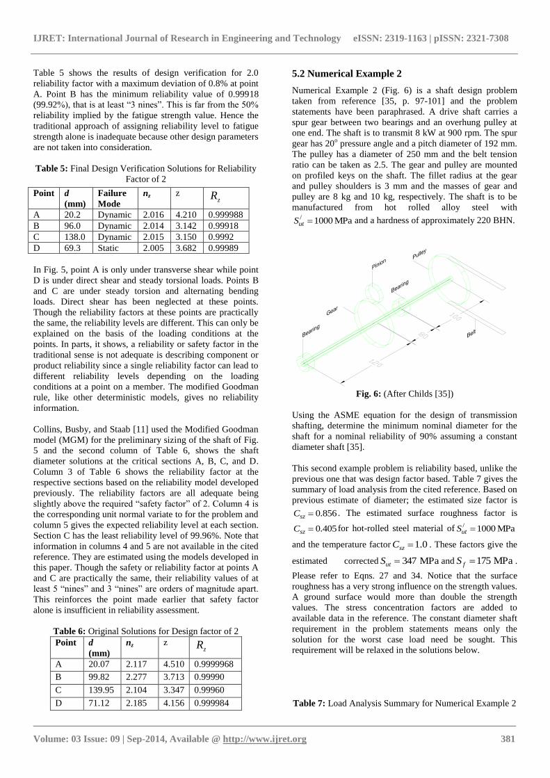
Numerical Example 2 (Fig. 6) is a shaft design problem

taken from reference [35, p. 97-101] and the problem

statements have been paraphrased. A drive shaft carries a

spur gear between two bearings and an overhung pulley at

one end. The shaft is to transmit 8 kW at 900 rpm. The spur

gear has 20o pressure angle and a pitch diameter of 192 mm.

The pulley has a diameter of 250 mm and the belt tension

ratio can be taken as 2.5. The gear and pulley are mounted

on profiled keys on the shaft. The fillet radius at the gear

and pulley shoulders is 3 mm and the masses of gear and

pulley are 8 kg and 10 kg, respectively. The shaft is to be

manufactured from hot rolled alloy steel with

MPa 1000/ utS and a hardness of approximately 220 BHN.

Fig. 6: (After Childs [35])

Using the ASME equation for the design of transmission

shafting, determine the minimum nominal diameter for the

shaft for a nominal reliability of 90% assuming a constant

diameter shaft [35].

This second example problem is reliability based, unlike the

previous one that was design factor based. Table 7 gives the

summary of load analysis from the cited reference. Based on

previous estimate of diameter; the estimated size factor is

856.0szC . The estimated surface roughness factor is

405.0szC for hot-rolled steel material of MPa 1000/ utS

and the temperature factor 0.1szC . These factors give the

estimated corrected MPa 347utS and MPa 175fS .

Please refer to Eqns. 27 and 34. Notice that the surface

roughness has a very strong influence on the strength values.

A ground surface would more than double the strength

values. The stress concentration factors are added to

available data in the reference. The constant diameter shaft

requirement in the problem statements means only the

solution for the worst case load need be sought. This

requirement will be relaxed in the solutions below.

Table 7: Load Analysis Summary for Numerical Example 2

Point d

(mm)

Failure

Mode

nz z

zR

A 20.2 Dynamic 2.016 4.210 0.999988

B 96.0 Dynamic 2.014 3.142 0.99918

C 138.0 Dynamic 2.015 3.150 0.9992

D 69.3 Static 2.005 3.682 0.99989


_______________________________________________________________________________________


Table 8 gives the initial or design sizing solutions at the

critical sections of the shaft while Table 9 gives the final or

design verification solutions. The diameter solution for the

worst case load section (Point C) in [35] is 32 mm.

Table 8: Initial Sizing Solutions for Numerical Example 2

Table 9: Final Verification Solutions for Numerical

Example 2

6. DISCUSSION

Tables 10a and 10b show a comparison between the initial

or design sizing solutions and the final or design verification

solutions. The initial solutions are always very slightly on

the conservative. This is due to the use of the design factor

which is an approximation of the reliability factor. Since the

initial diameter sizes are slightly conservative, surprising

changes in dimensions are not likely to arise during design

verification.

The second thing to appreciate about the models in this

paper is the closeness of the initial and final solutions. Most

of the reduction value is lower that 7% with only one size

being 11.3% smaller for Example 1. For this example, a trial

value of z = 3 was used to obtain a reliability value close to

2. This may explain this difference. Since a reliability target

was specified for the second example, no trial was

necessary. Because of this closeness, iterations in the design

verification task are fewer. This justifies one of the

motivating factors for the development of the model which

was to reduce design efforts.

It is appropriate at this point to compare solutions from the

references and the new solutions. This is done in Tables 11a

and 11b. For Example 1, the size reductions seem very

modest, and for Example 2, the reduction is relatively

substantial. These reductions could lead to potential savings

in costs associated with size, manufacturing, inspection,

assembly, and installation.

Table 10a: Initial and Final Shaft Diameter Sizes for

Example 1

Table 10b: Initial and Final Shaft Diameter Sizes for

Example 2

Table 11a: Previous and New Shaft Diameter Sizes for

Example 1

Table 11b: Previous and New Shaft Diameter Sizes for

Example 2

Point Fxy (N) Ma

(Nm)

Tm (Nm) k k

A 452.4 0 0 1.60 1.30

B 941.2 54.27 84.9 1.97 2.50

C 1588.0 158.8 84.9 1.60 1.30

D 2933.7 0 84.9 1.97 2.50

k and k are added by author

Point d

(mm)

no z

zR (%)

A 2.90 1.459 1.28 90

B 21.85 1.502 1.28 90

C 28.30 1.502 1.28 90

D 19.8 1.463 1.28 90

Point d (mm) nz z

zR (%)

A 2.70 1.282 1.439 92.6

B 21.00 1.408 1.279 90.6

C 27.60 1.407 1.296 90.2

D 18.50 1.307 1.370 91.54

Point Initial

d (mm)

Final

d (mm)

Reduction

(%)

A 21.70 20.2 6.9

B 102.61 96.0 6.4

C 143.65 138.0 3.9

D 78.10 69.3 11.3

Point Initial

d (mm)

Final

d (mm)

Reduction

(%)

A 2.90 2.70 6.9

B 21.85 21.00 3.9

C 28.30 27.60 2.5

D 19.8 18.50 6.6

Point Original

d (mm)

New

d (mm)

Reduction

(%)

A 20.07 20.2 2.4

B 99.82 96.0 3.8

C 139.95 138.0 1.4

D 71.12 69.3 2.6

Point Original

d (mm)

New

d (mm)

Reduction

(%)

A - 2.70 -

B - 21.00 -

C 32 27.60 13.8

D - 18.50 -


_______________________________________________________________________________________


For example, the bearing bore size based on the original

solution is 35 mm for Example 2. But the bearing bore size

based on the new solution is 30 mm. A ball bearing with 35

mm bore size will require larger bearing housing, retaining

ring, etc. than one with a 30 mm bore size. Hence if the

sizes estimated are satisfactory after considering other

serviceability criteria such as lateral deflection, torsional

deformation, critical whirling speed, and stability or

buckling resistance; substantial cost savings could result.

This is because smaller sizes are often easier and faster to

make and transport. The machining cost of components is

also influenced by size. To some extent, the inspection,

assembly, and maintenance costs are all influenced by size.

If the equipment is needed in large quantity, then thousands,

if not millions of dollars, could be saved due to smaller

sizes.

Both the Modified Goodman (MGM) and ASME models

allow reliability specification to be applied to the fatigue

strength. This study shows that the nominal reliability

specification may be quite different from the actual expected

value. The fact is that other design parameters are subject to

variations just as the fatigue strength. Hence the totality of

these parameter variations should be considered. Now a

nominal reliability of 50% seems to apply to Example 1

based on the MGM. However, the estimated expected

reliability is at least 99.96%. Also the nominal reliability for

Example 2 is 90% based on the ASME model, but the

estimated expected reliability is at least 99.92%. The gross

under estimation of reliability in these cases may be due

more to the MGM and ASME models’ conservative

positions relative to fatigue failure experimental data. MGM

is not close to average behavior of materials as the Gerber

fatigue model is [25]. The ASME model may not also be

close to the average behavior of materials in fatigue failure.

Because the new model can provide explicit reliability

values, it is an improvement on the MGM and ASME

models.

7. CONCLUSIONS

A reliability model has been developed for probabilistic

design. The model is applied to the design of a shaft loaded

in combined bending and torsion. In the reliability model, a

reliability factor is determined based on a target reliability

level, strength coefficient of variation, and stress coefficient

of variation. The stress coefficient of variations is estimated

using a first-order Taylor series expansion. The Gerber

bending fatigue rule was extended for applications in

combined bending and torsion using the concept of

equivalent bending loads. The shaft design method uses the

reliability factor in standard deterministic design formulas.

For initial design sizing, a design factor is approximated

from the reliability factor by simplifying the stress

coefficient of variation. For design verification, the expected

stresses are evaluated and used in the Gerber fatigue failure

equation to assess the reliability of the design. This design

approach simplifies the computational requirements of

probabilistic design and can help make probabilistic design

a common practice in machine design.

The examples considered show that size reductions are

possible with probabilistic design. Also explicit estimates of

reliability levels are possible. It was demonstrated that

nominal reliability level that specified only on the material

strength can be quite different from expected actual values

with some fatigue design models. Probabilistic design

provides quantitative risk assessment and permits reduction

in component sizes compared to deterministic approaches. It

avoids over- or under-design problems, leads to more

economical products, and help conserves scares and non-

renewable materials.

In reliability-based design, the reliability factor and

reliability level cannot be independently specified. The

target reliability level should be explicitly specified so that

the appropriate reliability factor can be determined. The

modified Goodman rule like other deterministic models;

gives no reliability information and can be conservative.

From Tables 6 and 9, it seems appropriate to conclude that

the approach outlined in this paper gives reasonable results.

It has the additional advantage of providing specific

reliability level information on a design. Also it

demonstrates that probabilistic design can be done with

cheap non-specialized software such as Microsoft Excel. It

is recommended that new equipment should be designed for

minimum size and weight while assuring reliability and

customer satisfaction by using reliability-based design

approaches.

ACKNOWLEDGEMENTS

This study was supported in parts with funds from COST

Faculty Development Fund of Texas Southern University,

Houston, Texas.

REFERENCES

[1]. Hammer, W. (1972), Handbook of System and Product

Safety, Prentice-Hall, Englewood Cliffs, N.J.

[2]. Zhang, Y. M., He, X D, Liu, Q L, and wen, B C, (2005),

An Approach of Robust Reliability Design for Mechanical

Components, Proc. IMechE, Vol. 219, part E. pg. 275 - 283.

Doi: 0.1243/095440805X8566. (http://www.paper.edu.cn).

[3]. Mott, R, L., (2008), Applied Strength of Materials, 5th

ed., Pearson Prentice Hall, Upper Saddle River, N.J.

[4]. ASME, (2007), Development of Reliability-Based Load

and Resistance Factor Design (LRFD) Methods for Piping,

ASME, New York, NY, pp. 2, 8.

[5]. Cullimore, B. and Tsuyuki, G., ( 2002), Reliability

Engineering and Robust Design: New Methods for

Thermal/Fluid Engineering, Proc., of 11th

Thermal and

Fluid Verification

[6]. Kalpakjian, S. and Schmid, S. R., (2001) Manufacturing

Engineering and Technology, 4th Ed. Pearson Prentice Hall,

Upper Saddle River, N.J.

[7]. Koch, P., (2002). Probabilistic Design: Optimization for

Six-Sigma Quality, 43rd

AIAA/ASME/ASCE/AHS/ASC

Conference. April 22 – 25. Denver, Colorado.

[8]. Shigley, J. E. & Mitchell, L. D., (1983), “Mechanical

Engineering Design”, McGraw-Hill, New York,

http://www.paper.edu.cn/


_______________________________________________________________________________________


[9]. Avoiding Common Mistakes and Misapplications in

Design for Reliability (DFR),

http://www.reliasoft.com/newsletter/v12i1/systhesis.htm.

[10]. Understanding Probabilistic Design,

http://www.kxcad.net/ansys/ANSYS/ansyshelp/Hlp_G_AD

VPDS1.html, Accessed 10-12-12.

[11]. Collins, A. J., Busby, H., and Staab, G., (2010),

Mechanical Design of Machine Elements, John Wiley &

Sons, New Jerey.

[12]. Juvinall, R. C. (1983), Fundamentals of Machine

Components Design, Wiley, New York, pp. 200 – 23

[13]. Shigley, J. E. and Mischke, C. R. (Chief Editors),

(1996), Standard Handbook of Machine Design, McGraw-

Hill, New York. p. 13.24 – 13.25

[14]. Socie, D, (2005), Probabilistic Aspects of Fatigue,

http://www.efatigue.com/training/probabilistic_fatigue.pdf

[15]. Ashby, F. M., & Jones, D. H. R. (1986). Engineering

Materials 2: An Introduction to Microstructure, Processing

and Design. Oxford, Pergamon.

[16]. Johnson, C. R. (1980), Optimum Design of Mechanical

Elements, Wiley, New York.

[17]. Shigley, J. E and Mischke, C. R. (Chief Editors),

(1996), Standard Handbook of Machine Design, McGraw-

Hill, New York.

[18]. Osakue, E. E. (2013), Probabilistic Design with

Gerber Fatigue Model, Mechanical Engineering Research,

Vol. 1, pp. 99 -117, doi:10.5539/mer.v3n1p99.

[19]. Agrawal, Avinash Chandra, (1971), On the

Probabilistic Design of Critical Engineering Components,

http://circle.ubc.ca/handle/2429/34397.

[20]. Pandit, S. M. and Shiekh, A. K., (1980), “Reliability

and Optimal Replacement via Coefficient of Variation,

Journal of Machine Design, Vol. 102, 761 -768.

[21]. Roshetov, D., Ivanov, A. and Fadeev, V. (1990),

Reliability of Machines, MIR, Moscow, Chap. 4.

[22]. Kravchenko, P. YE., (1964), Fatigue Resistance,

Pergamon, New York.

[23]. Sachs, N., (1999), Root Cause Failure Verification–

Interpretation of Fatigue Failures, Reliability Magazine,

August.

[24]. Hidgon, A., Ohseen, E. H., Stiles, W. B., and Weesa, J.

A., (1967), Mechanics of Materials, 2nd

. Ed. Wiley, New

York, Chap. 10.

[25]. Norton, R. L. (2000), Machine Design: An Integrated

Approach, Prentice-Hall, Upper Saddle River, New Jersey.

[26]. Mischke, C. R., (1996), Statistical Considerations, In

Standard Handbook of Machine Design, Shigley, J. E. and

Mischke, C. R. (Chief Editors), McGraw-Hill, New York.

[27]. Johnston, B. G., Lin, F. J., and Galambos, T. V.,

(1986), Basic Steel design, 3rd

ed., Prentice-Hall, Upper

Saddle River, New Jersey, p. 267.

[28]. Bausbacher, E. And Hunt, R. (1993), Process Plant

Layout and Piping Design, Prentice Hall, p. 271.

[29]. Lognormal Distribution, Engineering Statistics

Handbook,

http://itl.nist.gov/div898/handbook/eda/section3/eda3669.ht

m, Accessed April. 12, 2014

[30]. Osakue, E. E., Anetor, L. and Odetunde, C., (2012), A

Generalized Linearized Gerber Fatigue Model, Machine

Design, Vol. 4, ISSN 1821-1259, p. 1-10.

[31]. Wang, H., Kim, N. H., and Kim, Y., (2006), Safety

Envelope for Load Tolerance and its Application to Fatigue

Reliability, Journal of Mechanical Design, Vol. 128, pp. 919

– 927.

[32]. EPI Inc., (2008), “Metal Fatigue-Why Metal Parts Fail

from Repeatedly Applied Loads”.http://www.epi-

eng.com/mechanical_engineering_basics/fatigue_in_metals.

htm. Accessed 12-16-13.

[33]. Osakue, E. E. (2012), A Linearized Gerber Fatigue

Model, International Journal of Modern Engineering, Vol.

12, No 1, pp. 64 - 72.

[34]. Matthews, C. (2005). ASME Engineer’s Data Book, 2nd

ed. ASME Press, p.63 & 87.

[35]. Childs, P. R. N. (2004), Mechanical Design, 2nd

. ed.,

Elsevier, Asterdam, p. 97-101.

NOMENCLATURE

s service fatigue ratio

o basic fatigue ratio

load line slope factor

t load line slope transition factor

load line transition angle

a alternating bending load factor

m mean bending load factor

m mean bending service stress

a alternating bending service stress

m mean shear service stress

a alternating shear service stress

aeq equivalent alternating bending service stress

meq equivalent mean bending stress

ef effective bending stress

ef effective shear stress

k service bending stress concentration factor

/k theoretical bending stress concentration factor

k service shear stress concentration factor

/k theoretical shear stress concentration factor

xZ section modulus of member about x-axis

yZ section modulus of member about y-axis

pZ polar section modulus of member

mn mean stress ratio relative to tensile strength

an ratio of effective alternative stress to fatigue strength

xF shear force load in x-direction

yF shear force load in y-direction

xyF resultant shear force load in radial direction

minT minimum twisting moment value

maxT maximum twisting moment value

http://www.epi-eng.com/mechanical_engineering_basics/fatigue_in_metals.htm




_______________________________________________________________________________________


mT twisting moment mean value

aT twisting moment alternative value

minM minimum bending moment value

maxM maximum bending moment value

mM bending moment mean value

aM bending moment alternative value

meqM equivalent bending moment mean value

aeqM equivalent bending moment alternative value

d shaft solid diameter

z minor-to-major ratio of section moduli

fe fracture engineering strain on 50 mm gauge length

/fS laboratory test fatigue strength

fS service or corrected fatigue strength

/utS laboratory test ultimate tensile

utS service or corrected ultimate tensile strength

szC size adjustment factor

srC surface roughness adjustment factor

tpC temperature adjustment factor

S coefficient of variation of strength

ef coefficient of variation of effective normal stress,

ef

o coefficient of variation of basic fatigue ratio

no coefficient of variation of design factor

ov general overload coefficient of variation

bm local coefficient of variation of mean/alternating

bending moment

tm local coefficient of variation of mean/alternating

twisting moment,

zx coefficient of variation of section modulus

bmm local coefficient of variation of mean bending

moment

bma local coefficient of variation of alternating bending

moment

tmm local coefficient of variation of mean twisting

moment

tma local coefficient of variation of alternating twisting

moment

k coefficient of variation of service stress concentration

factor

dl coefficient of variation of the load due to local

dynamics

l coefficient of variation of member length

h coefficient of variation of cross-section depth h (same

for width b or diameter d)

mis miscellaneous coefficient of variation

ut service tensile strength coefficient of variation

fs service fatigue strength coefficient of variation

fb laboratory fatigue strength coefficient of variation

sz size coefficient of variation

sr surface roughness coefficient of variation

tp temperature coefficient of variation

su laboratory tensile strength coefficient of variation

a primary dependent random variable

i

x ith

independent random variable

y a secondary dependent random variable

f( ) = function of independent variables

S strength random variable

stress random variable

q failure stress lognormal random variable

mean value variable

S strength variable mean value

stress variable mean value

q

mean lognormal failure stress variable

S strength standard deviation

stress standard deviation

q lognormal failure stress standard

deviation

z unit normal variate

oz target unit normal variate

z

n design reliability factor at z

on design factor

zR reliability at z

cumulative probability density function

)(z normalized normal reliability function

)( z normalized normal un-reliability function

fr fillet radius

K generic factor

ovK general overload factor

K ratio of normal to shear stress

concentration factors

cba ,, functional indices

A, B, C, D: points on a shaft

APPENDIX

This Appendix discusses design factor, miscellaneous

variability and the estimate of reliability using the unit

normal variate.


_______________________________________________________________________________________


A1.1 Design Factor

Design involve uncertainties due to variability in loading

conditions, material properties, geometric properties,

accuracy of analytical models, fabrication and installation

precision, examination and inspection results, and in actual

usage [4]. Design uncertainties have been traditionally

handled through the use of safety or design factors. In

strength-stress based design, the design factor may be

defined as:

Stress Allowableor Design

Strengthon A1

The design factor is experiential and includes load and

material strength uncertainty [17]. The value of the design

factor is usually chosen by the designer based on experience

and judgment [3, Chap. 3]. In some situations, codes,

standards or company’s policy may specify design factors or

design stresses. In other situations, the designer must

carefully consider the nature and manner of loading, the

environment, material type (ductile or brittle), possible

failure and hazard (s), misuse or abuse, quality control,

market segment, accuracy of stress models, and cost. He or

she must make conservative estimates that will ensure that

the design is safe for all possible variations. An unduly high

design factor leads to over-design resulting in over-sized

components while an unduly low design factor leads to

under-design with higher risk of failure. It is wasteful to

purposely over-design and unwise to purposely under-

design.

In the approach presented in this paper, a design factor is

estimated using a simplified version of the equation for the

reliability factor for the purpose of initial sizing. This

approach ensures that a reasonable design factor based on

conditions similar but not identical to actual service

conditions is used in initial design. The design factor in this

case is solely a function of the reliability variable, the

variability of material strength and the variability of stress

model variables and factors. For dynamic fatigue design

sizing, the factor mn is assigned a value of 2. This

simplifies Eqn. 32 approximately to:

2

12222 )(5.0 mequtaeqmisno A2

In the static fatigue regime, the factor an is similarly

assigned a value of 2, and Eqn. 39 simplifies to:

2

1

2222 25.0 aeqfsmeqmisno A3

Then Eqn. 11 is used to obtain on as:

)1)(1(ln5.0

)1)(1(lnexp

22

22

nos

nosoo

zn

A4

A1.2 Miscellaneous Variability

The miscellaneous variability is considered to consist of

variability that is associated with design model formulation,

assembly, and installation operations. Simplified models in

engineering design have been in practice for over two

hundred years. They are generally sufficiently accurate to

about ±10% of reality [34]. The load experienced by

equipment in service depends on assembly accuracy and

proper installation. The influence of assembly and

installation practices on the variability of service load is not

easy to assess at the design phase, especially for new

products. The usual assumption is that these activities will

be done following standard or recommended practices but

actual practices may deviate from these. The variability due

to design model ( mod ), assembly ( ass ),, and installation (

ins ) activities may be assessed as:

222mod insassmis A5

Since engineering models are generally accurate to ±10%, a

model coefficient of variation ( mod ) of 5% is suggested.

Assuming that the assembly or installation variability is of

the same order as that of the design model variability,

respectively, then; 05.02

mod

22 insass. Hence from

Eqn. A5, an estimate of the miscellaneous cov is:

0866.005.005.005.0 222 mis A6

The effective value of the miscellaneous variability is

therefore taken as 085.0mis (8.5%).

A1.3 Reliability Estimate

The reliability estimate based on the unit normal variate is

commonly read from Tables given the value of the variate.

For use in a spreadsheet, it is more convenient to code a

formula. Using data from [13: p. 2.27], a curve fitting study

for 1.28 ≤ z < 7.0 for the unit normal curve yielded the

following:

3818.02299.02006.0 2 zzy A7

y

zR 101 A8

Equations A7 and A8 may be used to obtain reliability

values for known variate z instead of reading table values.

The range of reliability values is wide beginning from 90%

to 11 “nines”. Since table values are discrete, interpolation

may be needed occasionally. Using equations A7 and A8

avoids interpolation.