uncomplicated torsion and bending...

11th World Congress on Computational Mechanics (WCCM XI)5th European Conference on Computational Mechanics (ECCM V)

6th European Conference on Computational Fluid Dynamics (ECFD VI)E. Onate, J. Oliver and A. Huerta (Eds)

UNCOMPLICATED TORSION AND BENDING THEORIESFOR MICROPOLAR ELASTIC BEAMS

SOROOSH HASSANPOUR∗ AND G. R. HEPPLER†

∗Mechanical and Mechatronics EngineeringUniversity of Waterloo, Waterloo, ON, Canada N2L 3G1

e-mail: [email protected]

†Systems Design EngineeringUniversity of Waterloo, Waterloo, ON, Canada N2L 3G1

e-mail: [email protected]

Key words: Elastic Beam, Micropolar Elasticity, Torsion, Bending

Abstract. A simplified model for torsion and bending of 3D micropolar elastic beams isformulated first. The obtained static governing equations are solved numerically by usinga finite element approach and numerical examples are provided. Specially the conditionsunder which the results of the classical beam models are recovered will be presented.

1 INTRODUCTION

The origins of micropolar elasticity begin with Voigt’s work on adding an independentcouple stress vector to the classical force stress vector which was developed further by E.and F. Cosserat by suggesting independent displacement and microrotation fields, i.e. sixDOFs for every element of the body. Eringen extended the Cosserat theory to includemicroinertia effects and renamed it the micropolar theory of linear elasticty. A detailedreview of the micropolar theory of elasticity can be found in [1].

As in classical elasticity theory, it is useful to simplify the general micropolar theoryof linear elasticity to the special case of a micropolar beam, and to develop the microp-olar torsion and bending models for a micropolar beam. However, most of the existingmicropolar beam models, while being of interest, do not seem as convenient as classicalbeam torsion and bending models to a practitioner. For example, the torsion problemof micropolar elastic beams has been solved for both circular and noncircular cross sec-tions [2–5] and there are also papers on bending of the micropolar elastic beams [6–8];yet the complexity of these models is far beyond what is needed in a typical engineeringproblem. A simple model for the micropolar beam bending problem was developed byHaung [9] who, as an extension of the classical Euler-Bernoulli bending model, assumed

1

Soroosh Hassanpour and G. R. Heppler

that the shear deformations are negligible and the microrotations are equal to the bend-ing rotations of the beam plane sections. Another simple but more general model for themicropolar beam bending problem was addressed by Ramezani [10] who, as an extensionof the classical Timoshenko bending model, included the shear deformations and consid-ered the microrotations to be independent from the bending rotations. However, due tousing an incorrect definition for the strain tensor there are some errors in the equationspresented by Ramezani.

In this light the focus of this manuscript is to develop an uncomplicated but compre-hensive model to represent a micropolar beam deforming in 3D space. Such a model willemploy a simple longitudinal deformation theory combined with a generalized form ofDuleau torsion theory and an extended Timoshenko bending theory to characterize thetorsional and bending deformations of micropolar beams.

2 BACKGROUND

As noted previously, in micropolar elasticity model the displacement field vector →u andthe force stress tensor ↔σ are complemented by an independent microrotation field vector

→ϑ and a couple stress tensor↔χ . The potentially asymmetric strain tensor ↔ε and twist

(wryness or torsion) tensor↔τ are defined as:

εij = uj , i − εijk ϑk, τij = ϑj , i, (1)

and are related to the force and couple stresses via the micropolar constitutive relations:

σij =(µ+ κ

)εij +

(µ− κ

)εji + λ εkk 1ij,

χij =(γ + β

)τij +

(γ − β

)τji + α τkk 1ij,

(2)

where ↔1 is the second-order Kronecker (delta) tensor. The six elastic constants in Eq. (2)are the Lame coefficients µ and λ, and four micropolar elastic constants κ, γ , β , and α.Finally, in the micropolar elasticity theory, the elastic energy U takes the form:

U =

∫V

U V dV, U V =1

2σij εij +

1

2χij τij. (3)

3 KINEMATICS

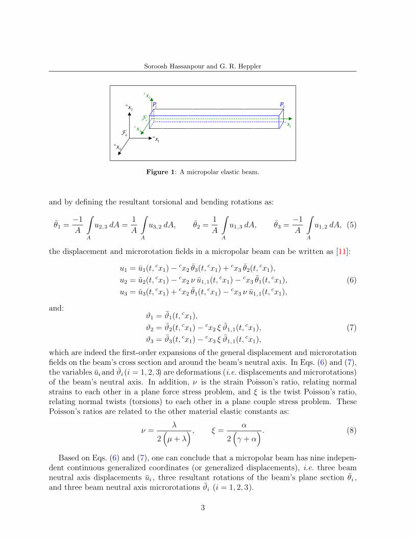
Consider the uniform beam in Figure 1 with an attached beam frame Fc at its leftend. The frame Fc is parallel to the inertial frame Fo and its first axis is coincide withthe beam neutral axis with boundary points P1 and P2 . The beam has length L , crosssection area A, polar moment of area I1, and principal second moments of area I2 and I3.

By assuming very small deformations through which the plane sections of the beamremain plane, the torsional warping effects on the cross section are negligible, and:

σ22 = σ33 = 0, χ22 = χ33 = 0, χ23 = χ32 = 0, ϑ1,2 = ϑ1,3 = 0, (4)

2


o

3

o x1

o x

2

o x

c

3

c x1

c x

2

c x

1P 2P

Figure 1: A micropolar elastic beam.

and by defining the resultant torsional and bending rotations as:

θ1 =−1

A

∫A

u2,3 dA =1

A

∫A

u3,2 dA, θ2 =1

A

∫A

u1,3 dA, θ3 =−1

A

∫A

u1,2 dA, (5)

the displacement and microrotation fields in a micropolar beam can be written as [11]:

u1 = u1(t, cx1)− cx2 θ3(t, cx1) + cx3 θ2(t, cx1),

u2 = u2(t, cx1)− cx2 ν u1,1(t, cx1)− cx3 θ1(t, cx1),

u3 = u3(t, cx1) + cx2 θ1(t, cx1)− cx3 ν u1,1(t, cx1),

(6)

and:ϑ1 = ϑ1(t, cx1),

ϑ2 = ϑ2(t, cx1)− cx2 ξ ϑ1,1(t, cx1),

ϑ3 = ϑ3(t, cx1)− cx3 ξ ϑ1,1(t, cx1),

(7)

which are indeed the first-order expansions of the general displacement and microrotationfields on the beam’s cross section and around the beam’s neutral axis. In Eqs. (6) and (7),the variables uiand ϑi (i = 1, 2, 3) are deformations (i.e. displacements and microrotations)of the beam’s neutral axis. In addition, ν is the strain Poisson’s ratio, relating normalstrains to each other in a plane force stress problem, and ξ is the twist Poisson’s ratio,relating normal twists (torsions) to each other in a plane couple stress problem. ThesePoisson’s ratios are related to the other material elastic constants as:

ν =λ

2(µ+ λ

) , ξ =α

2(γ + α

) . (8)

Based on Eqs. (6) and (7), one can conclude that a micropolar beam has nine indepen-dent continuous generalized coordinates (or generalized displacements), i.e. three beamneutral axis displacements ui , three resultant rotations of the beam’s plane section θi ,and three beam neutral axis microrotations ϑi (i = 1, 2, 3).

3


4 ELASTIC ENERGY EXPRESSION

Based on the results obtained in the previous section and by utilizing Eqs. (1), (2),and (3) the micropolar beam elastic energy expression takes the form [11]:

U =1

2E A

∫L

u1,1 u1,1 dL+1

2E I2

∫L

θ2,1 θ2,1 dL+1

2E I3

∫L

θ3,1 θ3,1 dL

+1

2µA

∫L

(u2,1 − θ3

)2

dL+1

2µA

∫L

(u3,1 + θ2

)2

dL

+1

2µ I1

∫L

θ1,1 θ1,1 dL

+1

2κA

∫L

(u2,1 + θ3 − 2 ϑ3

)2

dL+1

2κA

∫L

(u3,1 − θ2 + 2 ϑ2

)2

dL

+1

2κ I1

∫L

(θ1,1 − 2 ξ ϑ1,1

)2

dL+ 2κA

∫L

(θ1 − ϑ1

)2

dL

+1

2E A

∫L

ϑ1,1 ϑ1,1 dL+1

2

(γ + β

)A

∫L

(ϑ2,1 ϑ2,1 + ϑ3,1 ϑ3,1

)dL,

(9)

where µ is the shear modulus, E is the tensile (Young’s) modulus, relating the normalforce stresses to the normal strains in a plane force stress problem, and E is the tortile(torsional) modulus, relating the normal couple stresses to the normal twists (torsions) ina plane couple stress problem. The tensile and tortile moduli are defined as:

E =µ(

2µ+ 3λ)

µ+ λ= 2µ

(1 + ν

), E =

γ(

2 γ + 3α)

γ + α= 2 γ

(1 + ξ

). (10)

5 VIRTUAL WORK EXPRESSION

Assume that the micropolar beam shown in Figure 1 is under the action of externalvolume and boundary surface forces and moments

→f V , →m

V ,→f S , and →m

S (where bound-ary surface forces and moments are applied only on the most left and right beam crosssections). The virtual work expression for such a beam can be derived as [11]:

δW =

∫L

(A f

V

i δui + mL

i δθi + AmV

i δϑi

)dL

+ A fS

i (P1) δui(P1) + mP

i (P1) δθi(P1) + AmS

i (P1) δϑi(P1)

+ A fS

i (P2) δui(P2) + mP

i (P2) δθi(P2) + AmS

i (P2) δϑi(P2),

(11)

4


where:

A fV

i =

∫A

f V

i dA, A fS

i =

∫A

f S

i dA, A mV

i =

∫A

mV

i dA, A mS

i =

∫A

mS

i dA,

mL

1 =

∫A

(cx2 f

V

3 − cx3 fV

2

)dA, mL

2 =

∫A

cx3 fV

1 dA, mL

3 = −∫A

cx2 fV

1 dA,

mP

1 =

∫A

(cx2 f

S

3 − cx3 fS

2

)dA, mP

2 =

∫A

cx3 fS

1 dA, mP

3 = −∫A

cx2 fS

1 dA.

(12)

6 STATIC GOVERNING EQUATIONS

Upon applying the simplified Hamilton’s principle (or the principle of virtual work) onthe elastic energy and virtual work expressions and after adding the required correctionfactors (i.e. including ks2

and ks3as the shear correction factors and kt as the torsion

correction factor), the static governing equations for a micropolar beam will be obtainedas the following nine equations [11]:

A fV

1 + E A u1,11 = 0,

A fV

2 + ks2µA

(u2,11 − θ3,1

)+ κA

(u2,11 + θ3,1 − 2 ϑ3,1

)= 0,

A fV

3 + ks3µA

(u3,11 + θ2,1

)+ κA

(u3,11 − θ2,1 + 2 ϑ2,1

)= 0,

mL

1 + kt µ I1 θ1,11 + κ I1

(θ1,11 − 2 ξ ϑ1,11

)− 4κA

(θ1 − ϑ1

)= 0,

mL

2 + E I2 θ2,11 − ks3µA

(u3,1 + θ2

)+ κA

(u3,1 − θ2 + 2 ϑ2

)= 0,

mL

3 + E I3 θ3,11 + ks2µA

(u2,1 − θ3

)− κA

(u2,1 + θ3 − 2 ϑ3

)= 0,

A mV

1 + E A ϑ1,11 − 2 ξ κ I1

(θ1,11 − 2 ξ ϑ1,11

)+ 4κA

(θ1 − ϑ1

)= 0,

A mV

2 +(γ + β

)A ϑ2,11 − 2κA

(u3,1 − θ2 + 2 ϑ2

)= 0,

A mV

3 +(γ + β

)A ϑ3,11 + 2κA

(u2,1 + θ3 − 2 ϑ3

)= 0.

(13)

It is noteworthy that four modes of deformation are characterized by the relationsin Eq. (13); longitudinal displacement along the cx1 axis by the first relation, torsionalrotation around the cx1 axis by the fourth and seventh relations, lateral deformation inthe cx1

cx2 plane by the second, sixth, and ninth relations, and lateral deformation in thecx1

cx3 plane by the third, fifth, and eighth relations.The static equations given by Eq. (13) should be solved along with the following BCs

at boundary points P1 and P2 (where the “+” cases correspond to P1 and the “−” cases

5


correspond to P2):

δu1 = 0 or A fS

1 ± E A u1,1 = 0,

δu2 = 0 or A fS

2 ± ks2µA

(u2,1 − θ3

)± κA

(u2,1 + θ3 − 2 ϑ3

)= 0,

δu3 = 0 or A fS

3 ± ks3µA

(u3,1 + θ2

)± κA

(u3,1 − θ2 + 2 ϑ2

)= 0,

δθ1 = 0 or mP1 ± kt µ I1 θ1,1 ± κ I1

(θ1,1 − 2 ξ ϑ1,1

)= 0,

δθ2 = 0 or mP2 ± E I2 θ2,1 = 0,

δθ3 = 0 or mP3 ± E I3 θ3,1 = 0,

δϑ1 = 0 or AmS1 ± E A ϑ1,1 ± 2 ξ κ I1

(2 ξ ϑ1,1 − θ1,1

)= 0,

δϑ2 = 0 or AmS2 ±

(γ + β

)A ϑ2,1 = 0,

δϑ3 = 0 or AmS3 ±

(γ + β

)A ϑ3,1 = 0.

(14)

7 FINITE ELEMENT FORMULATION

A common numerical approach for solving the static equations in Eq. (13) is to use thevariational or weak form of the displacement-based FEM which is founded on the elas-tic energy and virtual work expressions. Here an isoparametric four-node element withC0 continuity and cubic Lagrange polynomial basis functions [12], which are integratedexactly, will be used to generate the consistent displacement-based finite element matri-ces. With these selections the shear locking is avoided [13, 14] and the completeness andcompatibility requirements of the FEM (monotonic) convergence are fulfilled [12].

The selected four-node element has four basis shape functions as:

H 〈1〉(ex1) = − 9

2 l3

(ex1 −

l

3

)(ex1 −

2 l

3

)(ex1 − l

),

H 〈2〉(ex1) = +27

2 l3ex1

(ex1 −

2 l

3

)(ex1 − l

),

H 〈3〉(ex1) = − 27

2 l3ex1

(ex1 −

l

3

)(ex1 − l

),

H 〈4〉(ex1) = +9

2 l3ex1

(ex1 −

l

3

)(ex1 −

2 l

3

),

(15)

where l and ex1 (0 ≤ ex1 ≤ l) are the element’s length and local frame coordinate respec-tively. Denoting the nodal coordinates by cx〈j〉i and the nodal generalized displacementsby q 〈j〉i , one can interpolate the within-element coordinates cxi, generalized displacementsqi , and the first space derivative of generalized displacements qi,1 as:

cxi = H 〈1〉 cx〈1〉i +H 〈2〉 cx〈2〉i +H 〈3〉 cx〈3〉i +H 〈4〉 cx〈4〉i ,

qi = H 〈1〉 q 〈1〉i +H 〈2〉 q 〈2〉i +H 〈3〉 q 〈3〉i +H 〈4〉 q 〈4〉i ,

qi,1 = H ′ 〈1〉 q 〈1〉i +H ′ 〈2〉 q 〈2〉i +H ′ 〈3〉 q 〈3〉i +H ′ 〈4〉 q 〈4〉i ,

(16)

6


where prime (i.e. �′) denotes the first spatial derivative with respect to ex1. Now one candefine the matrix of nodal generalized displacements

∼q 〈j〉 and the matrix of element(al)

generalized displacements∼q 〈e〉 as:

∼q 〈j〉 =

[q 〈j〉i]

=[u〈j〉1 u〈j〉2 u〈j〉3 θ

〈j〉1 θ

〈j〉2 θ

〈j〉3 ϑ

〈j〉1 ϑ

〈j〉2 ϑ

〈j〉3

]T,

∼q 〈e〉 =

[∼q 〈j〉]

=[∼q 〈1〉T

∼q 〈2〉T

∼q 〈3〉T

∼q 〈4〉T

]T

,(17)

which can be used to rewrite the expansion of qi in Eq. (16) as:

qi = ∼Hqi ∼q 〈e〉, (18)

where ∼Hqiare the shape function matrices of the forms:

∼H u1=[H 〈1〉

∼01×8H 〈2〉

∼01×8H 〈3〉

∼01×8H 〈4〉

∼01×8

],

∼H u2=[∼01×1

H 〈1〉∼01×8

H 〈2〉∼01×8

H 〈3〉∼01×8

H 〈4〉∼01×7

],

∼H u3=[∼01×2

H 〈1〉∼01×8

H 〈2〉∼01×8

H 〈3〉∼01×8

H 〈4〉∼01×6

],

∼H θ1=[∼01×3

H 〈1〉∼01×8

H 〈2〉∼01×8

H 〈3〉∼01×8

H 〈4〉∼01×5

],

∼H θ2=[∼01×4

H 〈1〉∼01×8

H 〈2〉∼01×8

H 〈3〉∼01×8

H 〈4〉∼01×4

],

∼H θ3=[∼01×5

H 〈1〉∼01×8

H 〈2〉∼01×8

H 〈3〉∼01×8

H 〈4〉∼01×3

],

∼H ϑ1=[∼01×6

H 〈1〉∼01×8

H 〈2〉∼01×8

H 〈3〉∼01×8

H 〈4〉∼01×2

],

∼H ϑ2=[∼01×7

H 〈1〉∼01×8

H 〈2〉∼01×8

H 〈3〉∼01×8

H 〈4〉∼01×1

],

∼H ϑ3=[∼01×8

H 〈1〉∼01×8

H 〈2〉∼01×8

H 〈3〉∼01×8

H 〈4〉].

(19)

By recalling Eqs. (9) and (11) and using the expansions of the form given by Eq. (18)and the shape functions given in Eq. (19) the virtual work and elastic energy expressionscorresponding to a micropolar beam element can be written as:

δW 〈e〉 = δ∼q 〈e〉

T

∼Q〈e〉, (20)

and:

U 〈e〉 =1

2 ∼q 〈e〉

T

∼K〈e〉

∼q 〈e〉, (21)

where∼Q〈e〉 is the finite element generalized force matrix:

∼Q〈e〉 =

∫l

(A ∼H

T

uif

V

i + ∼HT

θimL

i + A ∼HT

ϑimV

i

)dl

+∑P

(A ∼H

T

uif

S

i + ∼HT

θimP

i + A ∼HT

ϑimS

i

),

(22)

7


and ∼K〈e〉 is the finite element stiffness matrix:

∼K〈e〉 = E A

∫l

∼H′u1

T

∼H′u1dl + E I2

∫l

∼H′θ2

T

∼H′θ2dl + E I3

∫l

∼H′θ3

T

∼H′θ3dl

+ ks2µA

∫l

(∼H

′u2− ∼H θ3

)T (∼H

′u2− ∼H θ3

)dl

+ ks3µA

∫l

(∼H

′u3

+ ∼H θ2

)T (∼H

′u3

+ ∼H θ2

)dl + kt µ I1

∫l

∼H′θ1

T

∼H′θ1dl

+ κA

∫l

(∼H

′u2

+ ∼H θ3− 2 ∼H ϑ3

)T (∼H

′u2

+ ∼H θ3− 2 ∼H ϑ3

)dl

+ κA

∫l

(∼H

′u3− ∼H θ2

+ 2 ∼H ϑ2

)T (∼H

′u3− ∼H θ2

+ 2 ∼H ϑ2

)dl

+ κ I1

∫l

(∼H

′θ1− 2 ξ ∼H

′ϑ1

)T (∼H

′θ1− 2 ξ ∼H

′ϑ1

)dl

+ 4κA

∫l

(∼H θ1− ∼H ϑ1

)T (∼H θ1− ∼H ϑ1

)dl

+ E A∫l

∼H′ϑ1

T

∼H′ϑ1dl +

(γ + β

)A

∫l

(∼H

′ϑ2

T

∼H′ϑ2

+ ∼H′ϑ3

T

∼H′ϑ3

)dl.

(23)

8 RESULTS AND CONCLUSIONS

To provide numerical examples and make a comparison with the well-known classicalbeam models, the herein developed micropolar beam model is implemented in MATLAB®

[15] as a FEM model (with 16 elements, 4 nodes per element, and 9 DOFs per node) byusing the nondimensional parameters in Table 1. The nondimensional parameters given inTable 1 and the nondimensional displacements (used for reporting the results) are relatedto the micropolar beam’s dimensional parameters and displacements as:

Ri =

√AL2

Ii, µ =

µ

E, κ =

κ

E, γ =

γ

E L2, β =

β

E L2, ˆui =

uiL. (24)

The variations of the tip torsional rotations of a cantilevered micropolar beam subjectedto the action of an external body moment mV

1 with the variations of nondimensional pa-rameters κ and γ are shown in Figure 2. Analogous plots for the tip bending deformationsof a cantilevered micropolar beam under the action of external body force and moment

8


Table 1: Dimensionless parameters used in the numerical beam model.

Parameter R3 µ kt ks2ks3

κ γ = β ξ

Value 50 38 1 1 1 [10−10, 102] [10−10, 102] 1

2

fV

2 and mV

3 are depicted in Figures 3 and 4. In Figures 2–4 all the deformations arenormalized with respect to the deformations of a classical beam model (based on Duleautorsion and Timoshenko bending theories) under the action of the same load (obtainedfrom a FEM-based numerical model with 16 elements, 4 nodes per element, and 6 DOFsper node). The figures show the size-effect phenomenon [4] and the effect of choice ofmicropolar material constants κ and γ on the torsional and bending deformations of amicropolar beam. As expected large values of κ and γ result in more significant differencesbetween the micropolar and classical beam models. Large κ values and small γ values,on the other hand, result in a micropolar beam model that coincides with the classicalbeam model. The transition region is well defined and relatively abrupt (notice that theparameter scales are logarithmic). It is also interesting that the micropolar beam modelwith very small κ values shows singular behaviors when subjected to the action of anexternal volume moment. Note that the noisy behavior of the surface plots in the regionwhere κ� 1 and γ � 1 is due to an ill-conditioned FEM stiffness matrix and the inclusionof numerical precision errors.

Out of the many (or indeed infinite) possible micropolar beam models which can beobtained by varying κ and γ , five specific micropolar beam models are selected for amore thorough examination of the static deformations. In Figures 5 and 6 the completetorsional and bending deformations of five specific micropolar beam models under theaction of external moments mV

1 and mV

3 are plotted alongside with the torsional andbending deformations of a classical beam model (based on Duleau torsion and Timoshenkobending theories) under the action of the same load. The magnitude of the applied loadin each of Figures 5 and 6 (set of six plots) is selected to result in a maximum torsionalrotation or bending (nondimensional) displacement of 0.3 in the classical beam model.The singular behavior of a micropolar beam model with small κ values and the coincident-with-classical behavior of a micropolar beam model with large κ values and small γ valuesare more apparent in Figures 5 and 6.

REFERENCES

[1] W. Nowacki. Theory of asymmetric elasticity (translated by H. Zorski). Polish Sci-entific Publishers (PWN) & Pergamon Press, Warsaw, Poland & Oxford, UnitedKingdom, 1986.

[2] D. Iesan. Torsion of micropolar elastic beams. Int. J. of Eng. Sci., 9(11):1047–1060,

9


00.51

d a ta 1

-10-8

-6-4

-20

2

-10-8

-6-4

-20

2

0

50

100

log(γ)

R3 = 50

log(κ)

(θ1) m

p/(θ

1) c

l×

100

00.51

d a ta 1

-10-8

-6-4

-20

2

-10-8

-6-4

-20

2

0

50

100

log(γ)

R3 = 50

log(κ)

(ϑ1) m

p/(θ

1) c

l×

100

Figure 2: Relative tip torsional deformations of a cantilevered micropolar beam under volume momentmV

1 vs. micropolar elastic constants.

00.51

d a ta 1

-10-8

-6-4

-20

2

-10-8

-6-4

-20

2

0

50

100

log(γ)

R3 = 50

log(κ)

(ˆ u2) m

p/(ˆ u2) c

l×

100

00.51

d a ta 1

-10-8

-6-4

-20

2

-10-8

-6-4

-20

2

0

50

100

log(γ)

R3 = 50

log(κ)

(θ3) m

p/(θ 3) c

l×

100

00.51

d a ta 1

-10-8

-6-4

-20

2

-10-8

-6-4

-20

2

0

50

100

log(γ)

R3 = 50

log(κ)

(ϑ3) m

p/(θ 3) c

l×

100

Figure 3: Relative tip bending deformations of a cantilevered micropolar beam under volume force fV

2

vs. micropolar elastic constants.

00.51

d a ta 1

-10-8

-6-4

-20

2

-10-8

-6-4

-20

2

0

50

100

log(γ)

R3 = 50

log(κ)

(ˆ u2) m

p/(ˆ u2) c

l×

100

00.51

d a ta 1

-10-8

-6-4

-20

2

-10-8

-6-4

-20

2

0

50

100

log(γ)

R3 = 50

log(κ)

(θ3) m

p/(θ 3) c

l×

100

00.51

d a ta 1

-10-8

-6-4

-20

2

-10-8

-6-4

-20

2

0

50

100

log(γ)

R3 = 50

log(κ)

(ϑ3) m

p/(θ 3) c

l×

100

Figure 4: Relative tip bending deformations of a cantilevered micropolar beam under volume momentmV

3 vs. micropolar elastic constants.

10


00.51

d a ta 1

0 0.2 0.4 0.6 0.8 1-0.4

-0.2

0

0.2

0.4

Classical Model

R3 = 50

cx1

θ1

θ1-0.4

-0.2

0

0.2

0.4

θ1 00.51

d a ta 1

0 0.2 0.4 0.6 0.8 1-0.4

-0.2

0

0.2

0.4

Micropolar Model; κ = 102, γ = 10−10

R3 = 50

cx1

θ1

θ1-0.4

-0.2

0

0.2

0.4

ϑ1

ϑ1

00.51

d a ta 1

0 0.2 0.4 0.6 0.8 1-0.4

-0.2

0

0.2

0.4

Micropolar Model; κ = 10−10, γ = 10−10

R3 = 50

cx1

θ1

θ1-0.4

-0.2

0

0.2

0.4

ϑ1

ϑ1 × 10−7

00.51

d a ta 1

0 0.2 0.4 0.6 0.8 1-0.4

-0.2

0

0.2

0.4

Micropolar Model; κ = 102, γ = 102

R3 = 50

cx1

θ1

θ1-0.4

-0.2

0

0.2

0.4

ϑ1

ϑ1

00.51

d a ta 1

0 0.2 0.4 0.6 0.8 1-0.4

-0.2

0

0.2

0.4

Micropolar Model; κ = 10−10, γ = 102

R3 = 50

cx1

θ1

θ1-0.4

-0.2

0

0.2

0.4

ϑ1

ϑ1 × 10−6

00.51

d a ta 1

0 0.2 0.4 0.6 0.8 1-0.4

-0.2

0

0.2

0.4


R3 = 50

cx1

θ1

θ1-0.4

-0.2

0

0.2

0.4

ϑ1

ϑ1 × 10−1

Figure 5: Torsional deformations of a cantilevered beam under volume moment ˆmV

1 obtained fromdifferent classical and micropolar models.

00.51

d a ta 1

0 0.2 0.4 0.6 0.8 1-0.4

-0.2

0

0.2

0.4

Classical Model

R3 = 50

cx1

û2

û2

-0.8

-0.4

0

0.4

0.8

θ3

θ3

00.51

d a ta 1

0 0.2 0.4 0.6 0.8 1-0.4

-0.2

0

0.2

0.4

Micropolar Model; κ = 102, γ = 10−10

R3 = 50

cx1

û2

û2-0.8

-0.4

0

0.4

0.8

θ3&

ϑ3

θ3ϑ3

00.51

d a ta 1

0 0.2 0.4 0.6 0.8 1-0.4

-0.2

0

0.2

0.4


R3 = 50

cx1

û2

û2-0.8

-0.4

0

0.4

0.8

θ3&

ϑ3

θ3ϑ3 × 10−7

00.51

d a ta 1

0 0.2 0.4 0.6 0.8 1-0.4

-0.2

0

0.2

0.4

Micropolar Model; κ = 102, γ = 102

R3 = 50

cx1

û2

û2-0.8

-0.4

0

0.4

0.8

θ3&

ϑ3

θ3ϑ3

00.51

d a ta 1

0 0.2 0.4 0.6 0.8 1-0.4

-0.2

0

0.2

0.4

Micropolar Model; κ = 10−10, γ = 102

R3 = 50

cx1

û2

û2-0.8

-0.4

0

0.4

0.8

θ3&

ϑ3

θ3ϑ3 × 10−6

00.51

d a ta 1

0 0.2 0.4 0.6 0.8 1-0.4

-0.2

0

0.2

0.4


R3 = 50

cx1

û2

û2-0.8

-0.4

0

0.4

0.8

θ3&

ϑ3

θ3ϑ3 × 10−1

Figure 6: Bending deformations of a cantilevered beam under volume moment ˆmV

3 obtained fromdifferent classical and micropolar models.

11


1971.

[3] R.D. Gauthier and W.E. Jahsman. A quest for micropolar elastic constants. Tran.of the ASME, Series E-J. of Appl. Mech., 42(2):369–374, 1975.

[4] H.C. Park and R.S. Lakes. Torsion of a micropolar elastic prism of square cross-section. Int. J. of Sol. and Str., 23(4):485–503, 1987.

[5] S. Potapenko and E. Shmoylova. Weak solutions of the problem of torsion of micropo-lar elastic beams. Zeitschrift fur Angewandte Mathematik und Physik, 61(3):529–536,2010.

[6] R.D. Gauthier and W.E. Jahsman. Bending of a curved bar of micropolar elasticmaterial. Trans. of the ASME, Series E-J. of Appl. Mech., 43(3):502–503, 1976.

[7] G.V.K. Reddy and N.K. Venkatasubramanian. On the flexural rigidity of a microp-olar elastic cylinder. Trans. of the ASME, J. of Appl. Mech., 45(2):429–431, 1978.

[8] G.V.K. Reddy and N.K. Venkatasubramanian. On the flexural rigidity of a microp-olar elastic circular cylindrical tube. Int. J. of Eng. Sci., 17(9):1015–1021, 1979.

[9] F.Y. Huang, B.H. Yan, J.L. Yan, and D.U. Yang. Bending analysis of micropolarelastic beam using a 3-D finite element method. Int. J. of Eng. Sci., 38(3):275–286,2000.

[10] S. Ramezani, R. Naghdabadi, and S. Sohrabpour. Analysis of micropolar elasticbeams. Eur. J. of Mech.-A/Solids, 28(2):202–208, 2009.

[11] S. Hassanpour. Dynamics of Gyroelastic Continua. Ph.D. thesis, Mechanicaland Mechatronics Engineering Department, University of Waterloo, Waterloo, ON,Canada, 2014.

[12] K.J. Bathe. Finite element procedures in engineering analysis. Prentice-Hall, UpperSaddle River, NJ, United States, 1982.

[13] A.H. Vermeulen and G.R. Heppler. Predicting and avoiding shear locking in beamvibration problems using the b-spline field approximation method. Comp. Meth. inAppl. Mech. and Eng., 158(3):311–327, 1998.

[14] C.C. Richter and G.R. Heppler. L-spline finite elements. In ASME Int. Mech. Eng.Cong. and Exp., pages 147–156, Orlando, FL, USA, November 5-11 2005.

[15] MATLAB. 64-bit (win64), version 8.1.604 (R2013a). The MathWorks Inc., Natick,MA, United States, 2013. [Computer software].

12

uncomplicated torsion and bending...

Documents