Probabilistic Nearest Neighbor Queries on UncertainMoving Object Trajectories

Johannes Niedermayer∗, Andreas Zufle∗, Tobias Emrich∗,Matthias Renz∗, Nikos Mamouliso, Lei Chen+, Hans-Peter Kriegel∗

∗Institute for Informatics, Ludwig-Maximilians-Universitat Munchen{niedermayer,zuefle,emrich,kriegel,renz}@dbs.ifi.lmu.de

oDepartment of Computer Science, University of Hong Kongnikos@cs.hku.hk

+Department of Computer Science and Engineering, Hong Kong University of Science and Technologyleichen@cse.ust.hk

ABSTRACTNearest neighbor (NN) queries in trajectory databases have receivedsignificant attention in the past, due to their applications in spatio-temporal data analysis. More recent work has considered the realis-tic case where the trajectories are uncertain; however, only simpleuncertainty models have been proposed, which do not allow foraccurate probabilistic search. In this paper, we fill this gap by ad-dressing probabilistic nearest neighbor queries in databases withuncertain trajectories modeled by stochastic processes, specificallythe Markov chain model. We study three nearest neighbor querysemantics that take as input a query state or trajectory q and a timeinterval, and theoretically evaluate their runtime complexity. Fur-thermore we propose a sampling approach which uses Bayesianinference to guarantee that sampled trajectories conform to the ob-servation data stored in the database. This sampling approach canbe used in Monte-Carlo based approximation solutions. We includean extensive experimental study to support our theoretical results.

1. INTRODUCTIONWith the wide availability of satellite, RFID, GPS, and sensor

technologies, spatio-temporal data can be collected in a massivescale. The efficient management of such data is of great interestin a plethora of application domains: from structural and environ-mental monitoring and weather forecasting, through disaster/rescuemanagement and remediation, to Geographic Information Systems(GIS) and traffic control and information systems. In most currentresearch however, each acquired trajectory, i.e., the function of aspatio-temporal object that maps each point in time to a positionin space, is assumed to be known entirely without any uncertainty.However, the physical limitations of the sensing devices or limita-tions of the data collection process introduce sources of uncertainty.

Specifically, it is usually not possible to continuously capture theposition of an object for each point of time. In an indoor track-ing environment where the movement of a person is captured usingstatic RFID sensors, the position of the people in-between two suc-

This work is licensed under the Creative Commons Attribution-NonCommercial-NoDerivs 3.0 Unported License. To view a copy of this li-cense, visit http://creativecommons.org/licenses/by-nc-nd/3.0/. Obtain per-mission prior to any use beyond those covered by the license. Contactcopyright holder by emailing info@vldb.org. Articles from this volumewere invited to present their results at the 40th International Conference onVery Large Data Bases, September 1st - 5th 2014, Hangzhou, China.Proceedings of the VLDB Endowment, Vol. 7, No. 3Copyright 2013 VLDB Endowment 2150-8097/13/11.

cessive tracking events is not available ([1]). The same holds forgeo-social network (GSN) applications, where users have recentlybeen enabled to publicly share trajectories, such as bike routes1,tourist routes2 and GPS trajectories3. In many applications, the fre-quency of data collection is often decreased to save resources suchas battery power and wireless network traffic. Examples of tra-jectories with a relatively low frequency can be found on Bikely.Furthermore, traditional check-in data of GSN users often shows afrequency high enough to allow inference of a user’s position in be-tween discrete check-ins. Furthermore, incomplete (location, time)data is also collected in mobile object tracking applications. Forexample, in the T-Drive dataset ([3]) which consists of GPS-logsof taxis in Beijing, the time between two successive GPS measure-ments ranges from two seconds up to several minutes. In the Ge-oLife dataset ([4]), GPS observations of mobile users are loggedfrequently, usually every 1-5 seconds per point, while some ob-servations still have a lower sampling rate. All these datasets cre-ate a common challenge of interpolating the position of a user in-between discrete observations. In-between these observations theexact values are not explicitly stored in the database and are thusuncertain from the database perspective.

In this work, we consider a database D of uncertain moving ob-ject trajectories, where for each trajectory there is a set of observa-tions for only some of the history timestamps. Thus, the entire tra-jectory of an object is described by a time-dependent random vari-able, i.e., a stochastic process. Given a reference state or trajectoryq and a time interval T , we define probabilistic nearest-neighbor(PNN) query semantics, which are extensions of nearest neighborqueries in trajectory databases [5, 6, 7, 8]. Specifically, a P∃NNQ(P∀NNQ) query retrieves all objects in D, which have sufficientlyhigh probability to be the NN of q at one time (at the entire set oftimes) in T ; a probabilistic continuous NN (PCNNQ) query findsfor each object o ∈ D the time subsets Ti of T , wherein o has highenough probability to be the NN of q at the entire set of times inTi. Note that to the best of our knowledge this is the first approachthat tackles the PNN query problem correctly in consideration ofpossible worlds semantics.

PNN queries find several applications in analyzing historical tra-jectory data. For example, consider a geo-social network whereusers can publish their current spatial position at any time by so-called check-ins. For a historical event, users might want to find

1http://www.bikely.com/2http://www.everytrail.com/3http://www.gpsxchange.com, http://www.gpsshare.com/

205

their nearest friends during this event, e.g. to share pictures and ex-periences. As another application example, consider GPS-trackedtaxi cars as given in the T-Drive dataset [3] where PNN queries canbe used for analysis tasks like the assessment of taxi-client assign-ment procedures or for search tasks like searching for taxi driversthat might have observed a certain event like a car accident or acriminal activity such as a bank robbery. The taxi drivers that havebeen closest to the certain event location during the time the eventmight happened are potential witnesses. Note that this example ap-plication is used as our running application throughout this paper.

The main contributions of our work are as follows:• A thorough theoretical complexity analysis for variants of

probabilistic NN query problems.• A sampling-based approximate solution for all PNN prob-

lems which is based on Bayesian inference.• Thorough experimental evaluation of the proposed concepts

on real and synthetic data.The rest of the paper is structured as follows. Section 2 reviews

related work. Section 3 provides a formal problem definiton. Acomplexity analysis, approximate solutions and pruning techniquesof the proposed query semantics are provided in Sections 4-6. Anextensive experimental evaluation of the proposed techniques ispresented in Section 7. Section 8 briefly discusses general kNNqueries. Section 9 concludes this work.

2. RELATED WORKWithin the last decade, a considerable amount of research effort

has been put into query processing in trajectory databases (e.g. [8,9, 10, 11, 6]). In these works, the trajectories have been assumedto be certain, by employing linear [8] or more complex [9] typesof interpolation to supplement sparse observational data. How-ever, employing linear interpolation between consecutive observa-tions might create impossible patterns of movement, such as carstravelling through lakes or similar impossible-to-cross terrain. Fur-thermore, treating the data as uncertain and answering probabilisticqueries over them offers better insights4.

Uncertain Trajectory Modeling. Several models of uncertaintypaired with appropriate query evaluation techniques have been pro-posed for moving object trajectories (e.g. [12, 13, 14, 15]). Manyof these techniques aim at providing conservative bounds for thepositions of uncertain objects. This can be achieved by employ-ing geometric objects such as cylinders [13, 14] or beads [16] astrajectory approximations. While such approaches allow to answerqueries such as “is it possible for object o to intersect a query win-dow q”, they are not able to assign probabilities to these eventsconforming to possible worlds semantics.

Other approaches use independent probability density functions(pdf) at each point of time to model the uncertain positions of anobject [17, 14, 12]. However, as shown in [15], this may producewrong results (not in accordance with possible world semantics)for queries referring to a time interval because they ignore the tem-poral dependence between consecutive object positions in time. Tocapture such dependencies, recent approaches model the uncertainmovement of objects based on stochastic processes. In particular,in [18, 15, 1, 19], trajectories are modeled based on Markov chains.This approach permits correct consideration of possible world se-mantics in the trajectory domain.

Nearest Neighbor Queries in Trajectory Databases. In thecontext of certain trajectory databases there is not a common def-inition of nearest neighbor queries, but rather a set of different in-terpretations. In [5], given a query trajectory (or spatial point) q4http://infoblog.stanford.edu/2008/07/why-uncertainty-in-data-is-great-posted.html

and a time interval T , a NN query returns either the trajectory fromthe database which is closest to q during T or for each t ∈ T thetrajectory which is closest to q. The latter problem has also beenaddressed in [6]. Similarly, in [20], all trajectories which are near-est neighbors to q for at least one point of time t are computed.

Other approaches consider continuous nearest neighbor (CNN)semantics, definition of this query varies between publications [7,21, 8]. CNN have also been addressed for objects with uncertainvelocity and direction in [22]; the solutions proposed only find pos-sible results, but not result probabilities. Solutions for road networkdata were also proposed for the case where the velocities of objectsare unknown [23]. Furthermore, [14, 24] extended the problem ofcontinuous kNN queries (on historical search) to an uncertain set-ting, serving as important preliminary work, however, based on amodel which is not capable to return answers according to possibleworld semantics.

3. PROBLEM DEFINITIONA spatio-temporal database D stores triples (oi, time, location),

where oi is a unique object identifier, time ∈ T is a point in timeand location ∈ S is a position in space. Semantically, each suchtriple corresponds to an observation that object oi has been seen atsome location at some time. In D, an object oi can be described bya function oi(t) : T → S that maps each point in time to a locationin space; this function is called trajectory.

In this work, we assume a discrete time domain T = {0, . . . , n}.Thus, a trajectory becomes a sequence, i.e., a function on a discreteand ordinal scaled domain. Furthermore, we assume a discrete statespace of possible locations (states): S = {s1, ..., s|S|} ⊂ Rd, i.e.,we use a finite alphabet of possible locations in a d-dimensionalspace. The way of discretizing space is application-dependent: forexample, in traffic applications we may use road crossings, in in-door tracking applications we may use the positions of RFID track-ers and rooms, and for free-space movement we may use a simplegrid for discretization.

3.1 Uncertain Trajectory ModelLet D be a database containing the trajectories of |D| uncertain

moving objects {o1, ..., o|D|}. For each object o in D we storea set of observations Θo = {〈to1, θo1〉, 〈to2, θo2〉, . . . , 〈to|Θo|, θ

o|Θo|〉}

where toi ∈ T denotes the time and θoi ∈ S the location of observa-tion Θo

i . W.l.o.g. let to1 < to2 < . . . < to|Θo|. Note that the locationof an observation is assumed to be certain, while the location of anobject between two observations is uncertain.

According to [15], we can interpret the location of an uncertainmoving object o at time t as a realization of a random variableo(t). Given a time interval [ts, te], the sequence of uncertain loca-tions of an object is a family of correlated random variables, i.e., astochastic process. This definition allows us to assess the probabil-ity of a possible trajectory, i.e., the realization of the correspondingstochastic process. In this work we follow the approaches from [15,25, 19] and employ the first-order Markov chain model as a spe-cific instance of a stochastic process. The state space of the modelis the spatial domain S. State transitions are defined over the timedomain T . In addition, the Markov chain model is based on theassumption that the position o(t + 1) of an uncertain object o attime t+ 1 only depends on the position o(t) of o at time t. Clearly,this assumption is overly restrictive, as for example vehicles on aroad network will never follow a first-order Markov chain. Suchvehicles generally follow a best path (e.g. the shortest path or thepath having the most beautiful landscape, etc.). Nevertheless, sucha simplified model can, as we will see in our experimental evalua-tion, accurately model the set of possible trajectories that a vehicle

206

may have taken between two discrete observations. Theoretically,this high accuracy can be explained by combining both observationinformation and the Markov model into a new model.

The probability Moij(t) := P (o(t + 1) = sj |o(t) = si) is

the transition probability of a given object o from state si to statesj at a given time t. Transition probabilities are stored in a ma-trix Mo(t), called transition matrix of object o at time t. In gen-eral, every object o might have a different transition matrix, andthe transition matrix of an object might vary over time. Further, let~so(t) = (s1, . . . , s|S|)

T be the distribution vector of a given singleobject o at time t, where ~soi (t) = P (o(t) = si), i.e. each elementof the vector describes o’s probability of visiting the state si at timet. Without any further knowledge (from observations) the distribu-tion vector ~so(t + 1) can be inferred from ~so(t) by applying thefollowing formula: ~so(t+ 1) = Mo(t)T · ~so(t).

The traditional Markov model [15] uses forward probabilitiesonly. In Section 5, we propose a Bayesian inference approach,to condition this a-priori Markov chain to an adapted a-posterioriMarkov chain which also considers all observations of an object.

3.2 Nearest Neighbor QueriesIn this work we consider three types of time-parameterized NN

queries that take as input a certain reference state or trajectory q anda set of timesteps T . Note that q can be both a state or a trajectory,since a query state is simply a trivial query trajectory.

DEFINITION 1 (P∃NN QUERY). A probabil. ∃ nearest neigh-bor query retrieves all objects o ∈ D which have a sufficiently highprobability to be the nearest neighbor of q for at least one point oftime t ∈ T , formally:

P∃NNQ(q,D, T, τ) = {o ∈ D : P∃NN(o, q,D, T ) ≥ τ}where P∃NN(o, q,D, T ) =

P (∃t ∈ T : ∀o′ ∈ D \ o : d(q(t), o(t)) ≤ d(q(t), o′(t)))

and d(x, y) is a distance function defined on spatial points, typi-cally the Euclidean distance.

This definition is a extension of the spatio-temporal query pro-posed in [5] to the case of uncertainty. In the running taxi-trackingapplication mentioned in the introduction, the parameter T maycorrespond to the duration of a bank robbery, and q may corre-spond to the (constant) location of the bank, or the observed tra-jectory of the vehicle of the escaping robbers. In this application,a P∃NNQ(q,D, T, τ) query returns all taxis having a probabilityof at least τ of having been the closest cab at any time during therobbery, and thus, of possibly having observed something relevant.

In addition, we consider NN queries with the ∀ quantifier, whichhave also been proposed in [5] for crisp trajectory data.

DEFINITION 2 (P∀NN QUERY). A probabil. ∀ nearest neigh-bor query retrieves all objects o ∈ D which have a sufficiently highprobability (P∀NN ) to be the nearest neighbor of q for the entireset of timestamps T , formally:

P∀NNQ(q,D, T, τ) = {o ∈ D : P∀NN(o, q,D, T ) ≥ τ}where P∀NN(o, q,D, T ) =

P (∀t ∈ T : ∀o′ ∈ D \ o : d(q(t), o(t)) ≤ d(q(t), o′(t)))

In the running taxi-tracking application P∀NNQ(q,D, T, τ) re-turns all taxis having a probability of at least τ of having been theclosest cab during the whole robbery, and thus, of possibly havingobserved the whole crime scene. The main difference between Def-inition 1 and Definition 2 is that a P∃NNQ(q,D, T, τ) requires

s) bj t t j t P(t )

s

s3

s4

dist(q) object trajectory P(tr)

o1 tr1,1 = s2, s1, s1 0.5

o1 tr1 2 = s2 s3 s1 0.25

q

s1

s2o1 tr1,2  s2, s3, s1 0.25

o1 tr1,3 = s2, s3, s3 0.25

o2 tr2,1 = s3, s2, s2 0.5q

t1 2 3

o2 tr2,2 = s3, s4, s4 0.5

Figure 1: Example uncertain trajectories

a candidate object to be the nearest-neighbor of q for at least onepoint of time in T to qualify as a result, whileP∀NNQ(o, q,D, T )requires a candidate object to remain the nearest-neighbor for thewhole duration of T . In addition to these semantics for probabilisticnearest neighbor queries we now introduce a continuous query typewhich intuitively extends the spatio-temporal continuous nearest-neighbor query [21, 8] to apply on uncertain trajectories.

DEFINITION 3 (PCNN QUERY). A probabilistic continuousnearest neighbor query retrieves all objects o ∈ D together withthe set of timesets {Ti} where in each Ti the object has a suffi-ciently high probability to be always the nearest neighbor of q(t),formally:

PCNNQ(q,D, T, τ) =

{(o, Ti) : o ∈ D, Ti ⊆ T, P∀NN(o, q,D, Ti) ≥ τ}.

Analogously to the CNN query definition [21, 8], in order to re-duce redundant answers it makes sense to redefine the PCNN Querywhere we focus on results that maximize |Ti|, formally:

PCNNQ(q,D, T, τ) =

{(o, Ti) : o ∈ D,Ti ⊆ T, P∀NN(o, q,D, Ti) ≥ τ∧ ∀Tj ⊃ Ti : P∀NN(o, q,D, Tj) < τ}.

Note that according to this definition result sets Ti ⊆ T do nothave to be connected. In the taxi-tracking application, a PCNNQallows to find the set of time intervals in T where a taxi has a suf-ficiently high probability of being a witness. Such results allowto find groups of taxi drivers having a high probability of hav-ing witnessed the same part of the crime scene, in order to syn-chronize the evidence of multiple witnesses. To summarize, wehave defined three nearest-neighbor semantics for uncertain spatio-temporal data. All these semantics are inspired by correspondingnearest-neighbor semantics on certain trajectories, as defined in [5,21, 8].

EXAMPLE 1. To illustrate the three query types, consider thescenario shown in Figure 1 consisting of a query trajectory and twouncertain database objects D = {o1, o2} in a discretized spaceand time domain. For simplicity, whenever an object has two al-ternatives for choosing a possible state transition, each transitionis assumed to have a probability of 0.5. These probabilities de-fine the Markov chains of o1 and o2. Thus o1 has three possibletrajectories and o2 has two possible trajectories, the probabili-ties of which are also shown in Figure 1. Using possible worldssemantics, any PNN query can naively be computed by consid-ering all six possible combinations (tr1,i, tr2,j), i ∈ {1, 2, 3},j ∈ {1, 2}, called possible worlds, of possible trajectories of ob-jects o1 and o2. The total probability of all possible worlds whereo2 is closer to q than o1 at any time, by definition, equals the prob-ability P∃NN(o2, q,D, {1, 2, 3}). For this example these possi-ble worlds are (tr1,2, tr2,1) and (tr1,3, tr2,1). Assuming objectindependence, P (tr1,i, tr2,j) of a possible world is given by the

207

product P (tr1,i) ·P (tr2,j) yielding P∃NN(o2, q,D, {1, 2, 3}) =P (tr1,2) ·P (tr2,1)+ P (tr1,3) ·P (tr2,1) = 0.25 ·0.5+0.25 ·0.5 =0.25. Accordingly the probability P∀NN(o1, q,D, {1, 2, 3}) =0.75 can be computed by the sum of the probabilitiesP (tr1,1, tr2,1),P (tr1,1, tr2,2), P (tr1,2, tr2,2) andP (tr1,3, tr2,2) of worlds whereo1 is always closer to q than o2. A PCNNQ(q,D, {1, 2, 3}, 0.1)will return the object o1 together with the interval {1,2,3} and o2

together with the interval {2,3}, as in these intervals, the respectiveobjects have a probability of at least 0.1 to be closest to q.

In this example, exact probabilities are computed by explicit con-sideration of all possible worlds. However, since the number ofpossible trajectories grows exponentially large in the number oftime transitions, and the total number of possible worlds is fur-thermore exponential in the number of objects, the challenge ofthis work is to find a more efficient approach to compute the samenearest-neighbor probabilities without enumeration of all possibleworlds.

3.3 Query Evaluation Framework, RoadmapAn intuitive way to evaluate a PNN query is to compute for every

o ∈ D the probability P∃NN or P∀NN. However, to speed up queryevaluation, in Section 6, we show that it is possible to prune someobjects from consideration using an index over D. Then, for eachremaining object o, we have to compute a probability (i.e., P∃NNor P∀NN) and compare it to the threshold τ . In Section 4, we showthat computing the P∃NN query and P∀NN query is prohibitivelyexpensive. To solve this problem, in Section 5, we present a generalsampling-based approximate but efficient solution to solve all typesof PNN queries. As discussed in this section, P∃NN and P∀NN canbe approximated by Monte-Carlo simulation: for each object o′ ∈D a trajectory is generated which conforms to both the Markovchain modelMo′ and the observations Θo′ and all these trajectoriesare used to model a possible world. By performing the NN queryin all these possible worlds and averaging the results, we are ableto derive an approximate result probability.

4. THEORETICAL ANALYSISThis section theoretically studies the runtime complexity of the

P∃NNQ, P∀NNQ and PCNNQ queries.

4.1 The P∃NN QueryIn a P∃NNQ query, for any candidate object o ∈ D, Definition 1

requires the probability P∃NN(o, q,D, T ). However, the follow-ing lemma shows that this probability is hard to compute.

LEMMA 1. The computation ofP∃NN(o, q,D, T ) is NP-hard.

PROOF. P∃NN(o, q,D, T ) is equal to 1− P (¬∃t ∈ T,∀o′ ∈D\o : d(q(t), o(t)) ≤ d(q(t), o′(t))). We will show that decidingif there exists a possible world for which the expression:

¬∃t ∈ T,∀o′ ∈ D \ o : d(q(t), o(t)) ≤ d(q(t), o′(t)) (1)

is satisfied is an NP-hard problem. (Note that this is a much easierproblem than computing the actual probability.) Specifically, wewill reduce the well-known NP-hard k-SAT problem to the prob-lem of deciding on the existence of a possible world for which Ex-pression 1 holds.

For this purpose, we provide a mapping to convert a booleanformula in conjunctive normal form to a Markov chain modelingthe decision problem of Expression 1 in polynomial time. Thus,if the decision problem could be computed in PTIME, then k-SATcould also be solved in PTIME, which would only be possible if

P=NP. A k-SAT expressionE is based on a set of boolean variablesX = {x1, x2, . . . , xn}. The literal li of a variable xi is either xior ¬xi and a clause c =

∨xi∈C

li is a disjunction of literals where

C ⊆ X and |C| < k. ThenE is defined as a conjunction of clauses:E = c1 ∧ c2 ∧ . . . ∧ cm.

For our mapping, we will consider a simplified version of theP∃NN problem, specifically (1) q is a certain point, (2) o is a certainpoint and (3) the state space S of possible locations only includes4 states. As illustrated in Figure 2, compared to o, states s1 and s2

are closer to q and states s3 and s4 are further from q.5 Therefore,if an uncertain object is at states s1 or s2 then o is not the NN of q.

In our mapping, each variable xi ∈ X is equivalent to one un-certain object o′i ∈ D \ o. Furthermore each disjunctive clause cjis interpreted as an event happening at time t = j, i.e., the event c1happens at time t = 1, c2 happens at time t = 2 etc. Each clausecj can be seen as a disjunctive event that at least one object o′i attime t = j is closer to q than o (in this case, cj is true). Therefore,the conjunction of all these events, i.e. expression E =

∧1≤j≤m

cj ,

becomes true if the set of variables is chosen in a way that at eachpoint in time, compared to o, at least one object is closer to q; thisdirectly represents Expression 1. However, in k-SAT, not everyvariable xi (corresponding to o′i) is contained in each term cj whichdoes not correspond to our setting, since an uncertain object has tobe somewhere at each point in time. To solve this problem, we ex-tend each clause cj , such that each variable xi is contained in cj ,without varying the semantics of cj . Let us assume that xi is notcontained in cj . Then c′j = cj ∨ false = cj ∨ (xi ∧ ¬xi). Thismeans that we can assume that object o′i is definitely not closer toq than o at time t.

Let lji be the literal of variable xi in clause cj . Based on theabove discussion, we are able to construct for each object o′i twopossible trajectories (worlds). The first one, based on the assump-tion that xi is true, transitions between states s2 (if lji = true) ands4 (if lji = false). The second one, based on the assumption thatxi is set to false, transitions between states s1 (if lji = true) ands3 (if lji = false). Since these two trajectories can never be in thesame state it is straightforward to construct a time-inhomogeneousMarkov chain Mo(t) for each object o′i and each timestamp j.

After the Markov chains for each uncertain object o′i in D havebeen determined, we would just have to traverse them and computethe probability P∃NN(o, q,D, T ). If this probability is< 1, therewould exist a solution to the corresponding k-SAT formula. How-ever it is not possible to achieve this efficiently in the general caseas long as P 6= NP . Therefore computing P∃NN in subexpo-nential time is impossible.

Example: Consider a set of boolean variablesX = {x1, . . . , x4}and the following formula:

E = (¬x1 ∨ x2 ∨ x3) ∧ (x2 ∨ ¬x3 ∨ x4) ∧ (x1 ∨ ¬x2)

Therefore, we have

c1 = (¬x1∨x2∨x3), c2 = (x2∨¬x3∨x4) and c3 = (x1∨¬x2)

By employing the mapping discussed above, we get the four in-homogeneous Markov chains illustrated in Figure 2. For instance,under the condition that x1 is set to true, the value of the literal¬x1 is false at t = 1 (in clause c1) such that o′1 starts in the states4. On the other hand, if x1 is set to false, then o′1 starts in thestate s1.

5The states of o and q are omitted for the sake of simplicity.

208

s4t(q)

s

s3o

dist

x1 x2

q

s1

s2

q

t1 2 3x3 x4

Figure 2: An example instance of our mapping of the 3-SATproblem to a set of Markov chains.

In the second clause c2, since x1 6∈ C2, the position of o′1 mustnot affect the result. Therefore, for both cases x1 = false andx1 = true, o′1 must be behind o. In the last clause c3, if x1 = truethe object moves to state s2. On the other hand, if x1 = false, theobject moves to state s3.

4.2 The P∀NN QueryTheoretically showing the complexity of the P∀NNQ is more dif-

ficult than the analysis of the P∃NN query; the actual complexityof this type remains unknown. In the following we provide insightswhy P∀NN probabilities can not be computed efficiently. Let o ≺Tqoa denote the random predicate that is true iff object o is closer toq than object oa ∈ D during the query time T = [tstart, tend],i.e. ∀t ∈ T : d(o(t), q(t)) ≤ d(oa(t), q(t)). If o ≺Tq oa holds,we say that o dominates oa with respect to q during T . If the pa-rameters q and T are clear from the context, we simply say that odominates oa. Again we start our analysis by considering the sin-gle object probability P∀NN(o, q, {oa}, T ). This probability canbe computed correctly and efficiently.

LEMMA 2. The probability P (o ≺Tq oa) that o dominates oacan be computed in PTIME.

PROOF. We here provide just a basic proof sketch. In a nutshell,the idea of this proof is to treat objects o and oa as a single jointrandom variable having the joint transition matrix J(t) defined onthe state space S × S. Starting at t = tstart, time transitions ofJ(t) are performed iteratively. In each iteration, any entry of J(t)corresponding to a possible world where o does not dominate oaare set to zero. At time tend, the total probability of remainingworlds in J(tend) equals the probability that o dominates oa overthe whole duration of T .

Since this probability can be computed efficiently, we now ad-dress how to compute P∀NN(o, q,D, T ) for a whole database ef-ficiently, given that we can adapt the model of o to the dominationrelation o ≺Tq oa.

LEMMA 3. Given that a model (Mpost.i,j (t)) = P (o(t + 1) =

si|o(t) = sj , o ≺Tq oa) can be computed in PTIME, the probabilityP∀NN(o, q,D, T ) can be computed in PTIME.

PROOF. Again, a formal proof of this theorem can be found inthe extended version of this paper [26]. Here we will provide themain idea of the proof. By definition of predicate (o ≺Tq oa), wecan rewrite the probability that o is the nearest neighbor of q duringT as the following conjunctive formula: P∀NN(o, q,D, T ) =

P (∀oa ∈ D : o ≺Tq oa) = P (∧oa∈D

o ≺Tq oa). (2)

Clearly, Equation 2 follows from the fact that o is the NN of q ifand only if o is closer to q than all other objects in D during timeT . Using the chain rule of probability, which iteratively uses therule P (A∧B) = P (A) ·P (B|A) for conditional probabilities, weobtain

P (∧oa∈D

o ≺Tq oa) =∏

1≤a≤D

P (o ≺Tq oa|∧j<a

o ≺Tq oj). (3)

The first factor P (o ≺Tq o1) is given by Lemma 2. Now, byemploying the precondition of Lemma 3, we obtain an adaptedmodel of o given o ≺Tq o1. These two steps start the induc-tion. Now, given an adapted model of o given o ≺Tq o1, ..., o ≺Tqok, we can reapply Lemma 2 to compute P (o ≺Tq ok+1|o ≺Tqo1, ..., o ≺Tq ok) that the model of o, which has been adapted todominate o1, ..., ok, dominates ok+1. Next, we apply the precon-dition of Lemma 3 to take the current model of o, which has al-ready been adapted to o ≺Tq o1, ..., o ≺Tq ok, and further adaptthis model to o ≺Tq ok+1. Since both Lemma 2 and the precondi-tion of Lemma 3 can be computed in PTIME, P (

∧oa∈D o ≺

Tq oi),

which requires to apply Lemma 2 and the precondition of Lemma 3exactly |D| times, Lemma 3 can be computed in PTIME.

We still have to condition the a-priori model Mpriork,i (t − 1) =

P (o(t) = si|o(t − 1) = sk) of an object o to the event that odominates another object oa ∈ D, yielding modelMpost.

k,i (t−1) =

P (o(t) = si|o(t− 1) = sk, o ≺Tq oa). The problem here is, as wewill see, that the adapted model does not fulfil the Markov property,resulting in either exponential runtime or incorrect solutions.

To compute P (o(t) = si|o(t − 1) = sk, o ≺Tq oa), si, sk ∈S, the idea is to treat the positions of o and oa as a single jointstochastic process, having possible alternatives in S2. Then, thejoint a-priori transition matrixMo×oa(t) is conditioned to the evento ≺Tq oa following the forward-backward paradigm similar to theforward-backward approach used for sampling in Section 5. As aresult, we get a joint probability matrix Mo×oa(t− 1) =

P (o(t) = si, oa(t) = sj |o(t−1) = sk, oa(t−1) = sl, o ≺Tq oa)

Finally, in order to keep the complexity of this algorithm sub-exponential, we have to reduce this joint transition matrix to anadapted transition matrix Mpost.

k,i (t − 1) = P (o(t) = si|o(t −1) = sk, o ≺Tq oa) of object o. By applying the law of conditionalprobability, it can be shown that:

Mpost.k,i (t−1) =

∑sj

∑sl

P (oa(t−1) = sl|o(t−1) = sk, o ≺Tq oa)∗

P (o(t) = si, oa(t) = sj |o(t−1) = sk, oa(t−1) = sl, o ≺Tq oa)

Assuming that the Markov property still holds, we should get thesame results for

P (o(t) = si|o(t− 1) = sk, . . ., o(t− n) = st−n, o ≺Tq oa) =∑sj

∑sl

P (oa(t−1) = sl|o(t−1) = sk, . . ., o(t−n) = st−n, o ≺Tq oa)∗

P (o(t) = si, oa(t) = sj |o(t−1) = sk, oa(t−1) = sl, o ≺Tq oa)

which is clearly not equivalent, i.e. the Markov property does nothold on the reduced transition matrices and hence the algorithmhas exponential complexity. Therefore, in Section 5, we will pro-pose to use sampling to compute P∀NN(o, q,D, T ) probabilitiesefficiently.

209

4.3 The PCNN QueryThe traditional CNN query [21, 8], retrieves the nearest neigh-

bor of every point on a given query trajectory in a time intervalT . This basic definition usually returns m << |T | time intervalstogether having the same nearest neighbor. The main issue whenconsidering uncertain trajectories and extending the query defini-tion is the possibly large number of results due to highly over-lapping and alternating result intervals. In particular, consideringDefinition 3, a PCNN result may have an exponential number ofelements when τ becomes small. This is because in the worst caseeach Ti ⊆ T can be associated with an object o for which the prob-ability P∀NN(o, q,D, Ti) ≥ τ , i.e., 2T different Ti’s occur in theresult set.

To alleviate (but not solve) this issue, in the following we pro-pose a technique based on Apriori pattern mining to return the sub-sets of T that have a probability greater than τ . This algorithmrequires to compute a P∀NN probability in each validation step;we assume that this is achieved by employing the sampling ap-proach proposed in Section 5. Since each subset of T may have aprobability greater than τ (especially when τ is chosen too small),a worst-case of O(2n) validations may have to be performed.

Algorithm. Algorithm 1 shows how to compute, for a querytrajectory q, a time interval T , a probability threshold τ , and anuncertain trajectory o ∈ D all Ti ⊆ T for which o is the nearestneighbor to q at all timestamps in Ti with probability of at least τ ,and the corresponding probabilities.

Algorithm 1 PCτNN (q, o, D, T, τ )1: L1 = {({t}, P )|t ∈ T ∧ P = P∀NN(o, q,D \ {o}, {t}) ≥ τ}2: for k = 2;Lk−1 6= ∅; k + + do3: Xk = {Tk ⊆ T ||Tk| = k∧∀T ′k−1 ⊂ Tk∃(T

′k−1, P ) ∈ Lk−1}

4: Lk = {(Tk, P )|Tk ∈ Xk∧P = P∀NN(o, q,D\{o}, Tk) ≥ τ}5: end for6: return

⋃k Lk

We take advantage of the anti-monotonicity property that for aTi to qualify as a result of the PCNNQ query, all proper subsets ofTi must also satisfy this query. In other words if o is the P∀NN of qin Ti with probability at least τ , then for all Tj ⊂ Ti o must be theP∀NN of q in Tj with probability at least τ . Exploiting this prop-erty, we adapt the Apriori pattern-mining approach from [27] tosolve the problem as follows. We start by computing the probabili-ties of all single points of time to be query results (line 1). Then, weiteratively consider the set Xk of all timestamp sets with k pointsof time by extending timestamp sets Tk−1 with an additional pointof time t ∈ T \Tk−1, such that all T ′k−1 ⊂ Tk have qualified at theprevious iteration, i.e., we have P∀NN(o, q,D\{o}, T ′k−1)) ≥ τ(line 3).

The P∀NN probability is monotonically decreasing with the num-ber of points in time considered, i.e., P∀NN(o, q,D \ {o}, Tk) ≥P∀NN(q,D, Tk+1) where Tk ⊂ Tk+1. Therefore we do not haveto further consider the set of points of time Tk that do not qualifyfor the next iterations during the iterative construction of sets oftime points. Based on the sets of timesteps Tk constructed in eachiteration we compute P∀NN(o, q,D \ {o}, Tk) to build the set ofresults of length k (line 4) that are finally collected and reported asresult in line 6. The basic algorithm can be sped up by employingthe property that given P∀NN(o, q,D\{o}, T1) = 1 the probabilityof P∀NN(o, q,D \ {o}, T1 ∪ T2) = P∀NN(o, q,D \ {o}, T2).

Based on Algorithm 1 it is possible to define a straightforwardalgorithm for processing PCNNQ queries (by considering each ob-ject o′ from the database). Again this approach can be improved bythe use of an appropriate index-structure (cf. Section 6).

Figure 3: Traditional MC-Sampling.

Figure 4: An overview over our forward-backward-algorithm.

5. SAMPLING POSSIBLE TRAJECTORIESBased on the discussion in the previous sections, it is clear that

answering probabilistic queries over uncertain trajectory databaseshas high run-time cost. Therefore, like previous work [28], wenow study sampling-based approximate solutions to improve queryefficiency.

5.1 Traditional SamplingTo sample possible trajectories of an object, a traditional Monte-

Carlo approach would start by taking the first observation of theobject, and then perform forward transitions using the a-priori tran-sition matrix. This approach however, cannot directly account foradditional observations for latter timestamps. Figure 3 illustrates atotal of 1000 samples drawn in a one-dimensional space. Startingat the first observation time t = 0, transitions are performed us-ing the a-priori Markov chain. At the second observation at timet = 20, the great majority of trajectories becomes inconsistent.Such impossible trajectories have to be dropped. At time t = 40,even more trajectories become invalid; After this observation, onlyone out of a thousand samples remains possible and useful.

Clearly, the number of trajectory generations required to obtaina single valid trajectory sample increases exponentially in the num-ber of observations of an object, making this traditional Monte-Carlo approach inappropriate in obtaining a sufficient number ofvalid samples within acceptable time.

5.2 Efficient and Appropriate SamplingTo tackle the disadvantages of traditional sampling, we now in-

troduce an optimized approach af drawing samples. On these sam-ples, traditional NN algorithms for (certain) trajectories ([5, 6, 20,7, 21, 8]) can be used to estimate NN probabilities.

In a nutshell, our approach starts with the initial observation θo1at time to1, and performs transitions for object o using the a-prioriMarkov chain of o until the final observation θo|Θo| at time t|Θo|is reached. During this Forward-run phase, Bayesian inference isused to construct a time-reversed Markov model Ro(t) of o at timet given observations in the past, i.e., a model that describes theprobability

Roij(t) := P (o(t− 1) = sj |o(t) = si, {θoi |toi < t})

of coming from a state sj at time t−1, given being at state si at timet and the observations in the past. Then, in a second Backward-run phase, our approach traverses time backwards, from time t|Θo|

210

to t1, by employing the time-reversed Markov model Ro(t) con-structed in the forward phase. Again, Bayesian inference is used toconstruct a new Markov model F o(t− 1) that is further adapted toincorporate knowledge about observations in the future. This newMarkov model contains the transition probabilities

F oij(t− 1) := P (o(t) = sj |o(t− 1) = si,Θo). (4)

for each point of time t, given all observations, i.e., in the past, thepresent and the future.

As an illustration, Figure 4(left) shows the initial model givenby the a-priori Markov chain, using the first observation only. Inthis case, a large set of (time, location) pairs can be reached with aprobability greater than zero. The adapted model after the forwardphase (given by the a-priori Markov chain and all observations), de-picted in Figure 4(center), significantly reduces the space of reach-able (time, location) pairs and adapts respective probabilities. Themain goal of the forward-phase is to construct the necessary datastructures for efficient implementation of the backward-phase, i.e.,Ro(t). This task is not trivial, since the Markov property does nothold for the future, i.e., the past is not conditionally independentof the future given the present. Figure 4(right) shows the result-ing model after the backward phase. In the following section, bothphases are elaborated in detail.

Note that the Baum-Welch algorithm for hidden Markov mod-els (HMMs) is similar to the proposed algorithm. This algorithmaims at estimating time-invariant transition matrices and emissionprobabilities of a hidden Markov model. In contrast, we assumethis underlying model to be given, however we aim at adapting itby computing time-variant transition matrices. Despite these dif-ferences, the above algorithm could also be proven by showing thatour model is a special case of a HMM and deducting the algorithmfrom the Baum-Welch algorithm [30]. Related to our algorithmis also the Forward-Backward-Algorithm for HMMs that aims atcomputing the state distribution of an HMM for each point in time.In contrast, we aim at computing transition matrices for each pointin time, given a set of observations.

5.2.1 Forward-PhaseFirst note that, for the algorithm to work, it is necessary that ob-

servations are non-contradicting. To obtain the backward transitionmatrix Ro(t), we can apply the theorem of Bayes as follows:

Ro(t)ij := P (o(t− 1) = sj |o(t) = si) = (5)

P (o(t) = si|o(t− 1) = sj) · P (o(t− 1) = sj)

P (o(t) = si)

Computing Ro(t)ij is based on the a-priori Markov chain only,and does not consider any information provided by observations.To incorporate knowledge about past observations into Ro(t)ij , letpasto(t) := {θoi |toi < t} denote the set of observations temporallypreceding t. Also, let prevo(t) := argmaxΘo

i∈pasto(t)t

oi denote

the most recent observation of o at time t. Given all past observa-tions, Equation 5 becomes conditioned as follows:

LEMMA 4.

Ro(t)ij := P (o(t− 1) = sj |o(t) = si, pasto(t)) = (6)

P (o(t) = si|o(t− 1) = sj , pasto(t)) · P (o(t− 1) = sj |pasto(t))

P (o(t) = si|pasto(t))PROOF. Equation 6 uses the conditional theorem of Bayes

P (A|B,C) = P (B|A,C)·P (A|C)P (B|C)

, the correctness of which is shownin the extended version of this paper ([26]).

The conditional probability P (o(t) = si|o(t− 1) = sj , pasto(t))

can be rewritten as P (o(t) = si|o(t − 1) = sj), exploiting theMarkov property and the assumption of non-contradiction betweenmodel and observation.

By exploiting the Markov property, the priors P (o(t − 1) =sj |pasto(t)) and P (o(t) = si|pasto(t)) can both be rewritten asP (o(t − 1) = sj |prevo(t)) and P (o(t) = si|prevo(t)) respec-tively as long as o was not observed at time t; i.e., given the posi-tion at some time t, the position at a time t+ > t is conditionallyindependent of the position at any time t− < t. If o was observedat time t, this probabilty is trivially given by the observation. Thus,Equation 6 can be rewritten as Ro(t)ij =

P (o(t) = si|o(t− 1) = sj) · P (o(t− 1) = sj |prevo(t))P (o(t) = si|prevo(t))

(7)

The probability P (o(t) = si|o(t − 1) = sj) is given directlyby the definition of the a-priori Markov chain Mo(t) of o. Bothpriors P (o(t − 1) = sj |prevo(t)) and P (o(t) = si|prevo(t))can be computed by performing time transitions from observationprevo(t), also using the a-priori Markov chain Mo(t). For eachelement rij ∈ Roij(t), and each point of time t ∈ [t1, t|Θo|], thesepriors can be computed in a single run, iteratively performing tran-sitions from t1 to t|Θo|. During this run, all backward probabilitiesP (o(t − 1) = sj |o(t) = si, past

o(t)) are computed using Equa-tion 7 and memorized in the inhomogeneous matrix Ro(t). Duringany iteration of the forward algorithm, where a new observationpresento(t) := Θo

t ∈ Θo is reached, the information of this ob-servation has to be incorporated into the model. This is done triv-ially, by setting P (o(t) = si|pasto(t), presento(t)) to one if si isthe state θ observed by presento(t) and to zero otherwise.

5.2.2 Backward PhaseDuring the backward phase, we traverse time backwards using

the reverse transition matrix Ro(t), to propagate information aboutfuture observations back to past points of time, as depicted in Fig-ure 4(c). During this traversal, we again obtain a time reversedmatrix F o(t), describing state transitions between adjacent pointsof time, given observations in the future. Due to this second rever-sal of time, matrix F o(t) also contains adapted transition proba-bilities in the forward direction of time. Thus, matrix F o(t) repre-sents a Markov model which corresponds to the desired a-posteriorimodel: It contains the probabilities of performing a state transitionbetween state si and sj at time t to time t+1, incorporating knowl-edge of observations in both the past and the future. In contrast,the a-priori Markov modelMo(t) only considers past observations.We now discuss the details of this phase.

LEMMA 5. The following reverse Markov property holds foreach element Roij of Ro:

P (o(t) = sj |o(t+1) = si, o(t+2) = st+2, ..., o(t+k) = st+k) =

P (o(t) = sj |o(t+ 1) = si) (8)

This reverse markov property allows us to traverse the time domainbackward equivalent to a forward traversal. As an initial state forthe backward phase, we use the state vector corresponding to the fi-nal observation Θo

|Θo| at time to|Θo| at state θo|Θo|. This way, we takethe final observation as given, making any further probabilities thatare being computed conditioned to this observation. At each pointof time t ∈ [t|Θo|, t1] and each state si ∈ S, we compute the prob-ability that o is located at state si at time t given (conditioned to theevent) that the observations futureo(t) := {θoi |toi > t)} at timeslater than t are made. Let nexto(t) = argminΘo

i∈futureo(t)(t

oi )

211

denote the soonest observation of o after time t. To obtain F o(t),we once again exploit the theorem of Bayes:

F oij(t) := P (o(t+ 1) = sj |o(t) = si,Θo) =

P (o(t) = si|o(t+ 1) = sj ,Θo) · P (o(t+ 1) = sj |Θo)

P (o(t) = si|Θo)(9)

By exploiting the reverse Markov property (c.f. Equation 8), wecan rewrite P (o(t) = si|o(t+ 1) = sj ,Θ

o) = P (o(t) = si|o(t+1) = sj , past(t + 1)) which is given by matrix Ro(t). Both pri-ors P (o(t + 1) = sj |Θo) and P (o(t) = si|Θo) can be com-puted in the following way inductively. Given that we computeP (o(t) = si|past(t), present(t)) during the forward phase, thelast transition of the forward phase yields P (o(tend) = si|Θo).The remaining probabilities P (o(tk) = si|Θo) can be computedby employing the Markov transitions in backward direction withmatrix R(t).

5.2.3 Sampling Process

Algorithm 2 AdaptTransitionMatrices(o)1: {Forward-Phase}2: ~so(to1) = θo13: for t = to1 + 1; t ≤ to|Θo|; t++ do4: X′(t) = Mo(t− 1)T · diag(~so(t− 1))

5: ∀i ∈ {1 . . . |S|} : ~so(t)i =|S|∑j=1

X′ij(t)

6: ∀i, j ∈ {1 . . . |S|} : Ro(t)ij =X′

ij(t)

~so(t)i7: if t ∈ Θo then8: ~so(t) = θot {Incorporate observation}9: end if

10: end for11: {Backward-Phase}12: for t = to|Θo| − 1; t ≥ to1; t-- do13: X′(t) = Ro(t+ 1)T · diag(~so(t+ 1))

14: ∀i ∈ {1 . . . |S|} : ~so(t)i =|S|∑j=1

X′ij(t)

15: ∀i, j ∈ {1 . . . |S|} : F o(t)ij =X′

ij(t)

~so(t)i16: end for17: return F o

Algorithm 2 summarizes the construction of the transition modelfor a given object o. In the forward phase, the new distribution vec-tor ~so(t) of o at time t and backward probability matrix Ro(t) attime t can be efficiently derived from the temporary matrix X ′(t),computed in Line 4. The equation is equivalent to a simple tran-sition at time t, except that the state vector is converted to a di-agonal matrix first. This trick allows to obtain a matrix describ-ing the joint distribution of the position of o at time t − 1 andt. Formally, each entry X ′(t)i,j corresponds to the probabilityP (o(t − 1) = sj ∧ o(t) = si|pasto(t)) which is equivalent tothe numerator of Equation 6.6 To obtain the denominator of Eq.6 we first compute the row-wise sum of X ′(t) in Line 5. The re-sulting vector directly corresponds to ~so(t), since for any matrixA and vector x it holds that A · x = rowsum(A · diag(x)). Byemploying this rowsum operation, only one matrix multiplicationis required for computing Ro(t) and ~so(t).

Next, the elements of the temporary matrix X ′(t) and the ele-ments of ~so(t) are normalized in Equation 6, as shown in Line 6 ofthe algorithm.6The proof for this transformation P (A ∩ B|C) = P (A|C) ·P (B|A,C) can be derived analogously to Lemma 4.

Finally, possible observations at time t are integrated in Line 8.In Lines 12 to 15, the same procedure is followed in time-reverseddirection, using the backward transition matrix Ro(t) to computethe a-posteriori matrix F o(t).

The overall complexity of this algorithm is O(|T | · |S|2). Theinitial matrix multiplication requires |S|2 multiplications. Whilethe complexity of a matrix multiplication is in O(|S|3), the mul-tiplication of a matrix with a diagonal matrix, i.e., MT · s can berewritten as MT

i · sii, which is actually a multiplication of a vectorwith a scalar, resulting in an overall complexity of O(|S|2). Re-diagonalization needs |S|2 additions as well, such as re-normalizingthe transition matrix, yielding 3 · |T | · |S|2 for the forward phase.The backward phase has the same complexity as the forward phase,leading to an overall complexity of O(|T | · |S|2).

Once the transition matrices F o(t) for each point of time t havebeen computed, the actual sampling process is simple: For eachobject o, each sampling iteration starts at the initial position θo1 attime to1. Then, random transitions are performed, using F o(t) un-til the final observation of o is reached. Doing this for each objecto ∈ D, yields a (certain) trajectory database, on which exact NN-queries can be answered using previous work. Since the event thatan object o is a ∀NN (∃NN) of q is a binomial distributed randomvariable, we can use methods from statistics, such as the Hoeffd-ing’s inequality ([29]) to give a bound of the estimation error, for agiven number of samples.

6. SPATIAL PRUNINGPruning objects in probabilistic NN search can be achieved by

employing appropriate index structures available for querying un-certain spatio-temporal data. In this work, we use the UST-tree[25]. In this section, we briefly summarize the index and show howit can be employed to efficiently prune irrelevant database objects,identify result candidates, and find influence objects that might af-fect the ∀NN probability of a candidate object.

The UST-Tree. Given an uncertain spatio-temporal object o,the main idea of the UST-tree is to conservatively approximate theset of possible (location, time) pairs that o could have possiblyvisited, given its observations Θo. In a first approximation step,these (location, time) pairs, as well as the possible (location, time)pairs defined by Θo

i and Θoi+1 are minimally bounded by rectan-

gles. Such a rectangle, for observations Θoi and Θo

i+1 is definedby the time interval [toi , t

oi+1], as well as the minimal and maximal

longitude and latitude values of all reachable states.

EXAMPLE 2. Consider Figure 5, where four objects objects A,B, C and D are given by three observations at time 0, 5 and 10.For each object, the set of possible states in the corresponding timeintervals [0, 5] and [5, 10] is approximated by two minimum bound-ing rectangles. For illustration, the set of possible states at eachpoint of time is also depicted by dashed rectangles.

The UST-tree indexes the resulting rectangles using an R∗-tree([31]). We now discuss how such an index structure can be usedfor the evaluation of P∀NNQ and P∃NNQ queries.

Pruning candidates of P∀NNQ queries. For a P∀NNQ query,an object must have a non-zero probability of being the closest ob-ject to q, for all timestamps in the query interval. As a consequence,to find candidate objects for the P∀NNQ query, we have to considerfor all objects o ∈ D whether for each t ∈ q.T there does not existan object o′ ∈ D such that dmin(o(t), q(t)) > dmax(o′(t), q(t)).Here, dmin(o(t), q(t)) (dmax(o(t), q(t))) denotes the minimum(maximum) distance between the possible states of o(t) and q(t).Thus, the set of candidatesC∀(q) of a P∀NNQ is defined asC∀(q) =

212

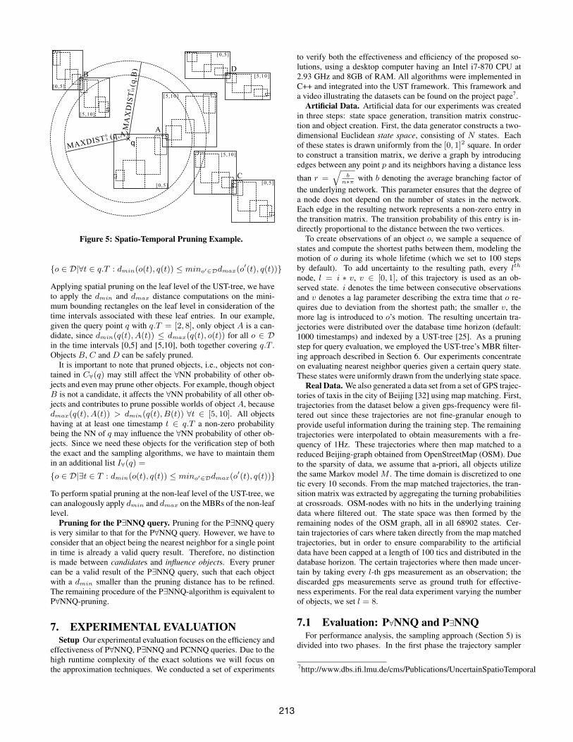
Figure 5: Spatio-Temporal Pruning Example.

{o ∈ D|∀t ∈ q.T : dmin(o(t), q(t)) ≤ mino′∈Ddmax(o′(t), q(t))}

Applying spatial pruning on the leaf level of the UST-tree, we haveto apply the dmin and dmax distance computations on the mini-mum bounding rectangles on the leaf level in consideration of thetime intervals associated with these leaf entries. In our example,given the query point q with q.T = [2, 8], only object A is a can-didate, since dmin(q(t), A(t)) ≤ dmax(q(t), o(t)) for all o ∈ Din the time intervals [0,5] and [5,10], both together covering q.T .Objects B, C and D can be safely pruned.

It is important to note that pruned objects, i.e., objects not con-tained in C∀(q) may still affect the ∀NN probability of other ob-jects and even may prune other objects. For example, though objectB is not a candidate, it affects the ∀NN probability of all other ob-jects and contributes to prune possible worlds of object A, becausedmax(q(t), A(t)) > dmin(q(t), B(t)) ∀t ∈ [5, 10]. All objectshaving at at least one timestamp t ∈ q.T a non-zero probabilitybeing the NN of q may influence the ∀NN probability of other ob-jects. Since we need these objects for the verification step of boththe exact and the sampling algorithms, we have to maintain themin an additional list I∀(q) =

{o ∈ D|∃t ∈ T : dmin(o(t), q(t)) ≤ mino′∈Ddmax(o′(t), q(t))}

To perform spatial pruning at the non-leaf level of the UST-tree, wecan analogously apply dmin and dmax on the MBRs of the non-leaflevel.

Pruning for the P∃NNQ query. Pruning for the P∃NNQ queryis very similar to that for the P∀NNQ query. However, we have toconsider that an object being the nearest neighbor for a single pointin time is already a valid query result. Therefore, no distinctionis made between candidates and influence objects. Every prunercan be a valid result of the P∃NNQ query, such that each objectwith a dmin smaller than the pruning distance has to be refined.The remaining procedure of the P∃NNQ-algorithm is equivalent toP∀NNQ-pruning.

7. EXPERIMENTAL EVALUATIONSetup Our experimental evaluation focuses on the efficiency and

effectiveness of P∀NNQ, P∃NNQ and PCNNQ queries. Due to thehigh runtime complexity of the exact solutions we will focus onthe approximation techniques. We conducted a set of experiments

to verify both the effectiveness and efficiency of the proposed so-lutions, using a desktop computer having an Intel i7-870 CPU at2.93 GHz and 8GB of RAM. All algorithms were implemented inC++ and integrated into the UST framework. This framework anda video illustrating the datasets can be found on the project page7.

Artificial Data. Artificial data for our experiments was createdin three steps: state space generation, transition matrix construc-tion and object creation. First, the data generator constructs a two-dimensional Euclidean state space, consisting of N states. Eachof these states is drawn uniformly from the [0, 1]2 square. In orderto construct a transition matrix, we derive a graph by introducingedges between any point p and its neighbors having a distance less

than r =√

bn∗π with b denoting the average branching factor of

the underlying network. This parameter ensures that the degree ofa node does not depend on the number of states in the network.Each edge in the resulting network represents a non-zero entry inthe transition matrix. The transition probability of this entry is in-directly proportional to the distance between the two vertices.

To create observations of an object o, we sample a sequence ofstates and compute the shortest paths between them, modeling themotion of o during its whole lifetime (which we set to 100 stepsby default). To add uncertainty to the resulting path, every lth

node, l = i ∗ v, v ∈ [0, 1], of this trajectory is used as an ob-served state. i denotes the time between consecutive observationsand v denotes a lag parameter describing the extra time that o re-quires due to deviation from the shortest path; the smaller v, themore lag is introduced to o’s motion. The resulting uncertain tra-jectories were distributed over the database time horizon (default:1000 timestamps) and indexed by a UST-tree [25]. As a pruningstep for query evaluation, we employed the UST-tree’s MBR filter-ing approach described in Section 6. Our experiments concentrateon evaluating nearest neighbor queries given a certain query state.These states were uniformly drawn from the underlying state space.

Real Data. We also generated a data set from a set of GPS trajec-tories of taxis in the city of Beijing [32] using map matching. First,trajectories from the dataset below a given gps-frequency were fil-tered out since these trajectories are not fine-granular enough toprovide useful information during the training step. The remainingtrajectories were interpolated to obtain measurements with a fre-quency of 1Hz. These trajectories where then map matched to areduced Beijing-graph obtained from OpenStreetMap (OSM). Dueto the sparsity of data, we assume that a-priori, all objects utilizethe same Markov model M . The time domain is discretized to onetic every 10 seconds. From the map matched trajectories, the tran-sition matrix was extracted by aggregating the turning probabilitiesat crossroads. OSM-nodes with no hits in the underlying trainingdata where filtered out. The state space was then formed by theremaining nodes of the OSM graph, all in all 68902 states. Cer-tain trajectories of cars where taken directly from the map matchedtrajectories, but in order to ensure comparability to the artificialdata have been capped at a length of 100 tics and distributed in thedatabase horizon. The certain trajectories where then made uncer-tain by taking every l-th gps measurement as an observation; thediscarded gps measurements serve as ground truth for effective-ness experiments. For the real data experiment varying the numberof objects, we set l = 8.

7.1 Evaluation: P∀NNQ and P∃NNQFor performance analysis, the sampling approach (Section 5) is

divided into two phases. In the first phase the trajectory sampler

7http://www.dbs.ifi.lmu.de/cms/Publications/UncertainSpatioTemporal

213

010203040506070

10000 100000 500000

CP

U T

ime

(s)

|S|

TS FA EX

0

10

20

30

40

50

60

10k 100k 500k

|C(q

)| an

d |I(

q)|

|S|

|C(q)| |I(q)|

Figure 6: Varying the Number of States N

010203040506070

6.0 8.0 10.0

CP

U T

ime

(s)

b

TS FA EX

02468

1012

6 8 10

|C(q

)| an

d |I(

q)|

b

|C(q)| |I(q)|

Figure 7: Varying the Branching Factor b

(TS) is initialized (the adapted transition matrices are computed ac-cording to Algorithm 2). This phase can be performed once andused for all queries. In the second phase, the actual sampling of10k trajectories (per object) for the approximate P∀NNQ (FA) andP∃NNQ (EX) queries is performed.

In our default setting during efficiency analysis on the artificialdataset we set the number of objects |D| = 10k, the number ofstates N = |S| = 100k, average branching factor of the syntheticgraph b = 8, probability threshold τ = 0 and the length of thequery interval |T | = 10. These parameters lead to a total of 110kobservations (11 per object) and 100k diamonds for the UST-index.

Varying N . In the first experiment (Figure 6) we investigate theeffect of an increasing state space size N , while keeping a constantaverage branching factor of network nodes. This effect correspondsto expanding the underlying state space, e.g., from a single countryto a whole continent. In Figure 6 (left) we can see that increasingN leads to a sublinear increase in the run-time of the samplingapproaches. This effect can be mostly explained by two aspects.First, the size of the a-priori model increases linearly withN , sincethe number of non-zero elements of the sparse matrix M increaseslinearly withN . This leads to an increase of the time complexity ofmatrix operations, and therefore makes adapting transition matricesmore costly. At the same time, the number of candidates |C(t)| andinfluence objects |I(t)| (see Section 6) decreases significantly asseen in Figure 6 (right) because the degree of intersection betweenobjects decreases with a higher number of states, making pruningmore effective, and therefore reducing the actual cost for sampling.

The runtime difference among sampling the P∀NNQ and P∃NNQquery diminishes with increasing N because the size of the resultset of the P∀NNQ increases with N while P∃NNQ produces lessresults with increasing N . The P∃NNQ runtime is also higher thanthe P∀NNQ runtime because for the P∃NNQ query not only candi-date objects are possible results, but also influence objects.

Varying b. Figure 7 evaluates the branching factor b, i.e., theaverage degree of each network node. As expected, Figure 7 (left)shows that an increasing branching factor yields a higher run-timeof all approaches due to a higher number of non-zero values in vec-tors and matrices, making computations more costly. Furthermore,in our setting, a larger branching factor also increases the numberof influence objects, as shown in Figure 7 (right).

Varying |D|. The number of objects (Figure 8) leads to a de-creasing performance as well. The more objects stored in a databasewith the same underlying motion model, the more candidates andinfluence objects are found during the filter step. This leads to anincreasing number of probability calculations during refinement,and hence a higher query cost.

01020304050607080

1000 10000 20000

CP

U T

ime

(s)

|D|

TS FA EX

0

5

10

15

20

1000 10000 20000

|C(q

)| an

d |I(

q)|

|D|

|C(q)| |I(q)|

Figure 8: Varying the Number of Objects |D|

020406080

100120140

1000 10000 20000

CP

U T

ime

(s)

|D|

TSFA

EX

0

10

20

30

40

50

1000 10000 20000

|C(q

)| an

d |I(

q)|

|D|

|C(q)| |I(q)|

Figure 9: Realdata: Varying the Number of Objects

Figure 10: Efficiency of Sampling without Model Adaption.

0

0.2

0.4

0.6

0.8

1

0 0.5 1

Est

imat

ed P

rob.

Reference Prob.

REFSASS

(a) P∀NN

0

0.2

0.4

0.6

0.8

1

0 0.5 1

Est

imat

ed P

rob.

Reference Prob.

REFSASS

(b) P∃NN

Figure 11: Effectiveness of Sampling, P∀NN and P∃NNReal Dataset. We conducted additional experiments to evaluate

P∀NNQ and P∃NNQ queries on the taxi dataset (Figure 9). The un-derlying state space consisting of 68902 states is a bit smaller thanthe default synthetic dataset. Based on this dataset, we ran an ex-periment varying the number of objects between 1000 and 20000.The smaller size of the state space leads to a higher objects density,leading to a larger number of candidates and influence objects thanthe corresponding experiment on the artificial dataset. Addition-ally, the non-uniform distribution of taxis in the city is more denseclose to the city center, making queries in this area more costlydue to the higher number of candidates and pruners. Further notethat in the real dataset, the motion patterns of objects are more di-verse than on the synthetic data. There are taxis standing still, andtaxis moving quite fast. Standing taxis have a larger area of un-certainty between observations, such that these objects reduce theperformance of query evaluation.

Sampling Efficiency. In the next experiment we evaluate theoverhead of the traditional sampling approach (using the a-prioriMarkov model only) compared to the approach presented in Sec-tion 5 which uses the a-posteriori model again based on the arti-ficial dataset. The first, traditional approach (TS1) discards anytrajectory not visiting all observations. As discussed in Section5.1, the expected number of attempts required to draw one samplethat hits all observations increases exponentially in the number ofobservations. This increase is shown in Figure 10, where the ex-pected number of samples is depicted with respect to the number

214

Figure 12: Realdata: Effectiveness of the Model Adaption

of observations. This approach can be improved, by segment-wisesampling between observations (TS2). Once the first observation ishit, the corresponding trajectory is memorized, and further samplesfrom the current observation are drawn until the next observation ishit. The number of trajectories required to be drawn in order to ob-tain one possible trajectory, i.e., the trajectory hits all observations,is linear to the number of observations when using this approach.We note in Figure 10, that in either approach at least 100k samplesare required even in the case of having only two observations. Incontrast using the approach presented in Section 5, the number oftrajectories that need to be sampled, in order to obtain a trajectorythat hits all observations, is always one.

Sampling Precision and Effectiveness. Next, we evaluate theprecision of our approximate P∀NNQ and P∃NNQ query and anaspect of a competitor approach [19]. The latter approach has beentailored for reverse NN queries, but can easily be adapted to NNquery processing. Essentially, this approach performs a snapshotquery P∀NNQ(q,D, {t}, τ) for each t ∈ T . P∀NN(o, q,D, T )is estimated by

∏t∈T P∀NN(o, q,D, {t}). P∃NN(o, q,D, T )

can be approximated by 1−∏t∈T (1−P∃NN(o, q,D, {t})). The

scatterplot in Figure 11 (right) illustrates a set of P∀NN probabiltieson synthetic data (v = 0.2, |T | = 5). For each experiment, weestimate probabilities by our sampling approach (SA) (Section 5)with (104) samples and by the adapted approach of [19] (SS). Weapproximated the exact approach (REF) by drawing a very high(106) number of samples.

We model each case as a (x,y) point, where x models the refer-ence (REF) and y the estimated probability (SA or SS). For (REF)the results always lie on the diagonal identity function depicted bya straight line. Probabilities of SA are very close to the diagonal,showing that our sampling solution tightly approximates the resultsof the exact P∀NNQ query. Concerning the snapshot approach, astrong bias towards underestimating probabilities can be observedfor the P∀NNQ query. The snapshot-based P∃NNQ-query overes-timates the results. This bias is a result of treating points of timemutually independent. In reality, the position at time t must be invicinity of the position at time t − 1, due to maximum speed con-straints. This positive correlation in space directly leads to a nearestneighbor correlation: If o is close to q at time t− 1, then o is likelyclose to q at time t. And clearly, if o is more likely to be close toq at time t, then o is more likely to be the NN of q at time t. Thiscorrelation is ignored by snapshot approaches. It can be seen thatthe systematic error of [19] is quite significant.

The number of samples required to obtain an accurate approx-imation of the probability of a binomial distributed random eventsuch as the event that o is the NN of q for each time t ∈ T has beenstudied extensively in statistics [29]. Thus the required number ofsamples is not explicitly evaluated here.

Effectiveness of the Forward-Backward Model. We tested theeffectiveness of the forward-backward model adaption in compari-son to other approaches on the real dataset with a time interval be-tween observations of 100 seconds. Figure 12 shows the mean errorof these approaches, computed during each point of time, evaluatedover a time interval of 30 tics (5 minutes). The mean error has been

020406080

100120140160

1000 10000 20000

CP

U T

ime

(s)

|D|

TSNNA

0200400600800

100012001400

1000 10000 20000

Tim

esta

mp

Set

s

|D|

#Timestamp Sets

Figure 13: PCNN: Varying the Number of Objects

computed in leave-one-out manner, i.e. trajectories for computingthe error have not been used to train the model in order to avoidoverfitting. The figure visualizes the error of the a-priori model(NO) considering only the first observation, the model adapted bythe forward phase only (F) and the forward-backward-adapted a-priori-model (FB) from this paper. We further implemented twoadditional approaches. The uniform approach (U), a competitorcorresponding to [13, 16], discards all probability information ofFB and, due to a lack of better knowledge, assumes all reachablestates at a given time to have a uniform probability. The differ-ence to the cylinders and beads approximation models presented in[13, 16] is that these models use conservative approximations thatmay include some (time, state) pairs actually having a zero prob-ability for an object to be located at. Thus, our U approach is atleast as good as the cylinders and beads approximation models interms of effectiveness, regardless of the approximation type used.The approach FBU is equivalent to FB, however turning proba-bilities in the transition matrix are equally distributed instead oflearning the exact transition probabilities from the underlying mapdata. First note that the approach not incorporating any observa-tions (NO), yields significant errors compared to the remaining ap-proaches. Clearly, observations can reduce errors and uncertaintyduring query evaluation. The forward-only approach (F) reducesthis error, however the error is still high especially directly beforean observation. This problem is solved by the forward-backwardapproach from this paper (FB). Note that even if the Markov chainis assumed to be uniformly distributed (FBU), the results are stillgood, but worse than with the actual learned probabilities (FB).This is good news, as it shows that even a non-optimally learnedMarkov chain can lead to useful results, however with a slightlyhigher error. This good performance comes from the fact that witha uniform transition distribution the diamond-shaped space of pos-sible time-state pairs still has high probabilities in the center of thediamond, since trajectories near the center of the bead will havea higher likelihood than trajectories close to the beads boundary.This stands in contrast to the uniform approach (U) that models allstates at the diamonds border to have the same probabilities as thestates in the diamonds center; explaining why U performs worsethan FBU. To conclude, combining observations with a sufficientlyaccurate transition matrix can produce the most accurate results.

7.2 Continuous QueriesIn our experimental evaluation on continuous queries we com-

pare the runtime and the size of the (unprocessed) result set for var-ious database sizes and values of the threshold τ (default τ = 0.5)using artificial data. After query evaluation, this result set can befurther condensed, e.g. by removing all smaller sets of timestampsthat are already implicitly contained in a larger set of timestamps.

Increasing the number of objects stored in the database leads toan increase in the time needed to compute the a-posteriori Markovmodel (TS) for each object (cf. Figure 13 (left)). This resultis equivalent to the result for P∀NNQ queries, since a-posteriorimodels have to be computed for either query semantics. However,the time required to obtain a sufficient number of samples (SA) is

215

0

50

100

150

200

0.1 0.5 0.9

CP

U T

ime

(s)

τ

TSSA

0100200300400500600700800

0.1 0.5 0.9

Tim

esta

mp

Set

s

τ

#Timestamp Sets

Figure 14: PCNN: Varying τ

much higher, since probabilities have to be estimated for a num-ber of sets of time intervals, rather than for the single interval T .This increase in run-time is alleviated by the effect that the numberof candidate time intervals obtained in the candidate time intervalgeneration step of our Apriori-like algorithm decreases (Figure 13(right)). This effect follows from the fact that more objects leadto more pruners, leading to smaller probabilities of time intervals,leading to fewer candidate time intervals. The results of varying τcan be found in Figure 14. Clearly an increasing probability thresh-old decreases the average size of the result (Figure 14 (right)). Con-sequently, the computational complexity of the query decreases asfewer candidates are generated. Figure 14(left) shows that the run-time of the sampling approach becomes very large for low values ofτ , since samples have to be generated for each relevant candidateset. Similar to the Apriori-algorithm, the number of such candi-dates grows exponentially with T , if τ is small.

8. K-NEAREST-NEIGHBOR QUERIESComputing P∀kNN and P∃kNN is NP-hard in k. Finally, the

C∀kNNQ query which is based on the ∀kNNQ query, is also NP-hard. The proof of this statement can be found in our technicalreport [26]. To answer P∃kNNQ queries, P∀kNNQ queries andPCkNNQ queries approximately in the case of k > 1, we can againutilize the model adaptation and sampling technique presented inSection 5. Therefore, possible worlds are sampled using the a-posteriori models of all objects, given their observations. On eachsuch (certain) world an existing solution for kNN search on certaintrajectories (e.g. [5, 6, 7, 8]) is applied. The results of these de-terministic queries can again be used to estimate the distribution ofthe probabilistic result.

9. CONCLUSIONSIn this paper, we addressed the problem of answering NN queries

in uncertain spatio-temporal databases. We proposed three differ-ent semantics of NN queries: P∀NNQ queries, P∃NNQ queriesand PCNN queries. We have first analyzed the complexity of thesequeries, showing that computing all of them has high runtime com-plexity. These results provide insights about the complexity ofNN search over uncertain data in general since the Markov chainmodel is one of the simplest models that consider temporal de-pendencies. More complex models are expected to be at least ashard. To mitigate the problems of computational complexity, weused a sampling-based approach based on Bayesian inference. Forthe PCNNQ query we proposed to reduce the cardinality of the re-sult set by means of an Apriori pattern mining approach. To copewith large trajectory databases, we introduced a pruning strategyto speed-up PNN queries exploiting the UST tree, an index for un-certain trajectory data. The experimental evaluation shows that ouradapted a-posteriori model allows to effectively and efficiently an-swer probabilistic NN queries despite the strong a-priori Markovassumption.

10. REFERENCES[1] C. Re, J. Letchner, M. Balazinksa, and D. Suciu, “Event queries on correlated

probabilistic streams,” in Proc. SIGMOD, 2008, pp. 715–728.[2] E. Cho, S. A. Myers, and J. Leskovec., “Friendship and mobility: User

movement in location-based social networks,” in Proc. KDD, 2001.[3] J. Yuan, Y. Zheng, C. Zhang, W. Xie, X. Xie, and Y. Huang, “T-drive: Driving

directions based on taxi trajectories,” in Proc. ACM GIS, 2010.[4] Y. Zheng, Q. Li, Y. Chen, X. Xie, and W. Ma., “Understanding mobility based

on gps data.” in Proc. Ubicomp, 2008, pp. 312–312.[5] E. Frentzos, K. Gratsias, N. Pelekis, and Y. Theodoridis, “Algorithms for

nearest neighbor search on moving object trajectories,” Geoinformatica,vol. 11, no. 2, pp. 159–193, 2007.

[6] R. H. Guting, T. Behr, and J. Xu, “Efficient k-nearest neighbor search onmoving object trajectories,” VLDB J., vol. 19, no. 5, pp. 687–714, 2010.

[7] G. S. Iwerks, H. Samet, and K. Smith, “Continuous k-nearest neighbor queriesfor continuously moving points with updates,” in VLDB, 2003, pp. 512–523.

[8] Y. Tao, D. Papadias, and Q. Shen, “Continuous nearest neighbor search,” inProc. VLDB, 2002, pp. 287–298.

[9] Y. Tao, C. Faloutsos, D. Papadias, and B. Liu, “Prediction and indexing ofmoving objects with unknown motion patterns,” in Proc. SIGMOD, 2004, pp.611–622.

[10] X. Yu, K. Q. Pu, and N. Koudas, “Monitoring k-nearest neighbor queries overmoving objects,” in Proc. ICDE, 2005, pp. 631–642.

[11] X. Xiong, M. F. Mokbel, and W. G. Aref, “Sea-cnn: Scalable processing ofcontinuous k-nearest neighbor queries in spatio-temporal databases,” in Proc.ICDE, 2005, pp. 643–654.

[12] H. Mokhtar and J. Su, “Universal trajectory queries for moving objectdatabases,” in Proc. MDM, 2004, pp. 133–144.

[13] G. Trajcevski, O. Wolfson, K. Hinrichs, and S. Chamberlain, “Managinguncertainty in moving objects databases,” ACM Trans. Database Syst., vol. 29,no. 3, pp. 463–507, 2004.

[14] G. Trajcevski, R. Tamassia, H. Ding, P. Scheuermann, and I. F. Cruz,“Continuous probabilistic nearest-neighbor queries for uncertain trajectories,”in Proc. EDBT, 2009, pp. 874–885.

[15] T. Emrich, H.-P. Kriegel, N. Mamoulis, M. Renz, and A. Zufle, “Queryinguncertain spatio-temporal data,” in Proc. ICDE, 2012, pp. 354–365.

[16] G. Trajcevski, A. N. Choudhary, O. Wolfson, L. Ye, and G. Li, “Uncertainrange queries for necklaces,” in Proc. MDM, 2010, pp. 199–208.

[17] R. Cheng, D. Kalashnikov, and S. Prabhakar, “Querying imprecise data inmoving object environments,” in IEEE TKDE, vol. 16, no. 9, 2004, pp.1112–1127.

[18] S. Qiao, C. Tang, H. Jin, T. Long, S. Dai, Y. Ku, and M. Chau, “Putmode:prediction of uncertain trajectories in moving objects databases,” Appl. Intell.,vol. 33, no. 3, pp. 370–386, 2010.

[19] C. Xu, Y. Gu, L. Chen, J. Qiao, and G. Yu, “Interval reverse nearest neighborqueries on uncertain data with markov correlations,” in Proc. ICDE, 2013.

[20] G. Kollios, D. Gunopulos, and V. Tsotras, “Nearest neighbor queries in amobile environment,” in Spatio-Temporal Database Management. Springer,1999, pp. 119–134.

[21] A. Prasad Sistla, O. Wolfson, S. Chamberlain, and S. Dao, “Modeling andquerying moving objects,” in Proc. ICDE. IEEE, 1997, pp. 422–432.

[22] Y.-K. Huang, S.-J. Liao, and C. Lee, “Efficient continuous k-nearest neighborquery processing over moving objects with uncertain speed and direction,” inProc. SSDBM, 2008, pp. 549–557.

[23] G. Li, Y. Li, L. Shu, and P. Fan, “Cknn query processing over moving objectswith uncertain speeds in road networks,” in APWeb, 2011, pp. 65–76.

[24] G. Trajcevski, R. Tamassia, I. F. Cruz, P. Scheuermann, D. Hartglass, andC. Zamierowski, “Ranking continuous nearest neighbors for uncertaintrajectories,” VLDB J., vol. 20, no. 5, pp. 767–791, 2011.

[25] T. Emrich, H.-P. Kriegel, N. Mamoulis, M. Renz, and A. Zufle, “Indexinguncertain spatio-temporal data,” in Proc. CIKM, 2012, pp. 395–404.

[26] J. Niedermayer, A. Zufle, T. Emrich, M. Renz, N. Mamoulis, L. Chen, and H.-P.Kriegel, “Probabilistic nearest neighbor queries on uncertain moving objecttrajectories (technical report),” 2013,http://www.dbs.ifi.lmu.de/Publikationen/Papers/TR PNN.pdf.

[27] R. Agrawal and R. Srikant, “Fast algorithms for mining association rules,” inProc. VLDB, 1994, pp. 487–499.

[28] R. Jampani, F. Xu, M. Wu, L. L. Perez, C. M. Jermaine, and P. J. Haas, “Mcdb:a monte carlo approach to managing uncertain data,” in Proc. SIGMOD, 2008,pp. 687–700.

[29] W. Hoeffding, “Probability inequalities for sums of bounded random variables,”Journal of the American Statistical Association, pp. 13–30, 1963.

[30] L. R. Welch, “Hidden markov models and the baum-welch algorithm,” IEEEInformation Theory Society Newsletter, vol. 53, no. 4, pp. 1,10–13, 2003.

[31] N. Beckmann, H.-P. Kriegel, R. Schneider, and B. Seeger, “The R*-Tree: Anefficient and robust access method for points and rectangles,” in Proc.SIGMOD, 1990.

[32] J. Yuan, Y. Zheng, X. Xie, and G. Sun, “Driving with knowledge from thephysical world,” in Proc. KDD, 2011, pp. 316–324.

216