probabilistic validation of homology computations for...

The Annals of Applied Probability2007, Vol. 17, No. 3, 980–1018DOI: 10.1214/105051607000000050© Institute of Mathematical Statistics, 2007

PROBABILISTIC VALIDATION OF HOMOLOGY COMPUTATIONSFOR NODAL DOMAINS

BY KONSTANTIN MISCHAIKOW1 AND THOMAS WANNER2

Rutgers University and George Mason University

Homology has long been accepted as an important computable tool forquantifying complex structures. In many applications, these structures ariseas nodal domains of real-valued functions and are therefore amenable only toa numerical study based on suitable discretizations. Such an approach imme-diately raises the question of how accurate the resulting homology compu-tations are. In this paper, we present a probabilistic approach to quantifyingthe validity of homology computations for nodal domains of random fields inone and two space dimensions, which furnishes explicit probabilistic a prioribounds for the suitability of certain discretization sizes. We illustrate our re-sults for the special cases of random periodic fields and random trigonometricpolynomials.

1. Introduction. The practical need to extract low-dimensional nonlinearstructures from high-dimensional data sets has led to the introduction of topologi-cal methods in statistical analysis. There is a growing body of literature [10, 13, 14,26, 28] that addresses the problem of providing efficient algorithms for estimatingtopological properties of a fixed, but unknown, manifold X given a point-clouddata set that lies on or near X. The equally important complementary question isthat of the accuracy of these estimations. To the best of our knowledge, the first re-sult is due to Niyogi, Smale and Weinberger [25]. In this paper, the authors proposea stochastic algorithm for computing the homology of a given manifold X ⊂ R

d

by randomly sampling M points from the manifold and derive explicit bounds onthe probability that their algorithm computes the correct homology. The proba-bility bound depends on the number M and a condition number 1/τ . The latterparameter encodes both local curvature information of the manifold X and globalseparation properties. More precisely, the inverse condition number τ is the largestnumber such that the open normal bundle about X ⊂ R

d of radius r is embeddedin R

d for all r < τ .Although stimulated by the aforementioned results, the motivation for the work

presented in this paper comes from the study of patterns produced by nonlinear

Received September 2006; revised December 2006.1Supported in part by NSF Grants DMS-05-11115 and DMS-01-07396, by DARPA and the

U.S. Department of Energy.2Supported in part by NSF Grant DMS-04-06231 and the U.S. Department of Energy under Con-

tract DE-FG02-05ER25712.AMS 2000 subject classifications. 60G60, 55N99, 60G15, 60G17.Key words and phrases. Homology, random fields, nodal domains.

980

http://www.imstat.org/aap/

http://dx.doi.org/10.1214/105051607000000050

http://www.imstat.org

http://www.ams.org/msc/

PROBABILISTIC VALIDATION OF HOMOLOGY COMPUTATIONS 981

evolutionary systems such as phase separation in materials, fluid flow and pop-ulation biology. While the mathematical models for such systems are typicallyinfinite-dimensional, understanding the time evolution of the multitude of oftencomplicated patterns produced on an underlying two- or three-dimensional do-main is of considerable, if not primary, interest. As is described in greater detailbelow, algebraic topology and, in particular, computational homology can be usedto obtain new statistical measurements for either numerical or experimental dataassociated with these spatially and temporally complex systems [18, 19, 23]. Asabove, the accuracy of these homology computations is an important question.However, because the data is obtained through numerical methods or by standardimaging techniques, the data points are not naturally modeled via a random sam-pling, but rather appear on a fixed grid. On the other hand, the patterns are con-stantly changing and thus one is interested in the topology of a multitude of man-ifolds. Furthermore, at those points in time for which the topology of the patternchanges, the condition number 1/τ becomes unbounded.

These observations suggest the need for a complementary result concerning theaccuracy of homology computations. To be more precise, consider a compact rec-tangular domain G := [a, b]d ⊂ R

d and a smooth function u ∈ C2(G,R). Thenodal domains of u are given by the sub- and super-level sets

N± := {x ∈ G :±u(x) ≥ 0},which can be interpreted as patterns on the domain G. These are the objects whichwe wish to identify through their homology, that is, we are interested in the statis-tics of H∗(N±) as the functions u vary.

Given the limitations of numerical and imaging (think digital camera) tech-niques, the nodal domains must be approximated. The following provides a rea-sonable model for such an approximation.

DEFINITION 1.1 (Cubical approximation of a nodal domain). Considera compact rectangular domain G := [a, b]d ⊂ R

d and a continuous functionu :G → R. Let M be an arbitrary positive integer. Define the equidistantM-discretization of [a, b] as the collection of grid points

xk := a + k · b − a

M, for k = 0, . . . ,M.

The cubical approximations Q±M of the nodal domains N± = {x ∈ G :±u(x) ≥ 0}

are defined as the sets

Q±M := ⋃{

d∏�=1

[k�, k� + 1] :±u(x1,k1, . . . , xd,kd) ≥ 0, k ∈ {0, . . . ,M}d

},

where k = (k1, . . . , kd) and where xj,0, . . . , xj,M denotes the equidistantM-discretization of the j th component interval of G. For the case of one-dimensional domains, this definition is illustrated in Figure 1; for the two-dimensional case, see Figure 2.

982 K. MISCHAIKOW AND T. WANNER

FIG. 1. Nodal domain approximation using cubical sets in one dimension.

At first glance, one might expect that for sufficiently smooth functions u andsufficiently large discretization size M , the homologies of the nodal domains N±and of their cubical approximations Q±

M would coincide. Simple counterexamplesto this exist; however, this assertion can be made correct from a probabilistic pointof view.

Consider a probability space (�,F ,P) and let u :G×� → R denote a randomfield over (�,F ,P) such that for P-almost all ω ∈ �, the function u(·,ω) :G → R

is twice continuously differentiable. We will impose the following two assump-tions throughout this paper:

(A1) for every x ∈ G, we have P{u(x) = 0} = 0;

FIG. 2. Nodal domains of a random trigonometric polynomial in two space dimensions and theircubical approximations with M = 50.


(A2) the random field is such that P{0 is a critical value of u} = 0.

To simplify the notation, we follow the customary procedure of dropping the ex-plicit ω-dependence in the formulation of events, that is, we write, for example,P{u(x) = 0} instead of P({ω ∈ � :u(x,ω) = 0}).

THEOREM 1.2. Consider a probability space (�,F ,P), a domain G :=[a, b]d ⊂ R

d and a random field u :G × � → R over (�,F ,P) such that forP-almost all ω ∈ �, the function u(·,ω) :G → R is twice continuously differen-tiable. For each ω ∈ �, denote the nodal domains of u(·,ω) by N±(ω) ⊂ G andgiven a positive integer M , denote their cubical approximations by Q±

M(ω).If both (A1) and (A2) are satisfied, then for P-almost all ω ∈ �, the following

holds. For all sufficiently large values of M , the homology of the cubical approxi-mations Q±

M(ω) matches that of the nodal domains N±(ω). In other words, thereexists a random variable M :� → N such that

P{For all M ≥ M one has H∗(N±) ∼= H∗(Q±M)} = 1.

Note that the random variable M is in general neither constant nor bounded.

REMARK 1.3. One can show that in the situation of Theorem 1.2, there ac-tually exists a homeomorphism h :G → G which is isotopic to the identity suchthat h(N±) = Q±

M . In other words, the nodal sets and their cubical approximationsare homeomorphic. Similar extensions are also valid for our probabilistic main re-sults. Nevertheless, in view of the current state of applications, we present all ofour results within the homology setting.

We do not provide an explicit proof of this result since it follows from the re-alization that for P-almost all ω ∈ �, the level set u(x,ω) = 0 is a manifold withfinite condition number 1/τ < ∞ and a straightforward modification of the proofof [25], Proposition 3.1, then readily furnishes the above result.

Observe that the hypotheses for Theorem 1.2 provide a fairly general frameworkin which to study the topology of random manifolds. However, the motivation forthis work leads us in a slightly different direction. As an example, consider theproblem of phase separation in binary metal alloys. During the last few decades,many models have been proposed for describing this process. Starting from thecelebrated Cahn–Hilliard partial differential equation model [8, 9], numerous ex-tensions and refinements have been proposed over the years. While all of thesemodels are infinite-dimensional evolution equations they can be deterministic orstochastic partial differential equations and can contain nonlocal or other addi-tional terms. Moreover, all of these models are phenomenological models in thesense that while they are based on important physical insights, they are not rigor-ously derived from first principles and so assessing the quality of a specific modelbecomes a central and crucial problem. Since the material microstructures which


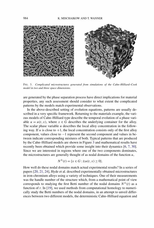
FIG. 3. Complicated microstructures generated from simulations of the Cahn–Hilliard–Cookmodel in two and three space dimensions.

are generated by the phase separation process have direct implications for materialproperties, any such assessment should consider to what extent the complicatedpatterns by the models match experimental observations.

In the above-described setting of evolution equations, patterns are usually de-scribed in a very specific framework. Returning to the materials example, the vari-ous models of Cahn–Hilliard type describe the temporal evolution of a phase vari-able u = u(t, x), where x ∈ G describes the underlying container for the alloy.The scalar phase variable u describes the local alloy concentration in the follow-ing way. If u is close to +1, the local concentration consists only of the first alloycomponent, values close to −1 represent the second component and values in be-tween indicate corresponding mixtures of both. Typical patterns that are producedby the Cahn–Hilliard models are shown in Figure 3 and mathematical results haverecently been obtained which provide some insight into their dynamics [6, 7, 30].Since we are interested in regions where one of the two components dominates,the microstructures are generally thought of as nodal domains of the function u,

N±(t) = {x ∈ G :±u(t, x) ≥ 0}.How well do these nodal domains match actual experimental results? In a series ofpapers [20, 21, 24], Hyde et al. described experimentally obtained microstructuresin iron-chromium alloys using a variety of techniques. One of their measurementswas the handle number of the structure which, from a mathematical point of viewcorresponds to studying the first Betti number of the nodal domains N±(t) as afunction of t . In [19], we used methods from computational homology to numeri-cally study the Betti numbers of the nodal domains, in an attempt to unveil differ-ences between two different models, the deterministic Cahn–Hilliard equation and


the stochastic Cahn–Hilliard–Cook model. Since the underlying nonlinear evolu-tions were solved numerically, we do not have direct access to the nodal domains.However, for a fixed grid size bounded from below by the resolution used in thenumerical approximation, the associated cubical approximation is easily obtained.

This last comment indicates the limitations of Theorem 1.2. Ideally, given anevolution equation and a fixed cubical approximation of the nodal domain, wewould like to be able to estimate the amount of time for which the homology com-putations of the nodal domains are correct. This problem appears to be extremelydifficult. Thus we pose the following, simpler, goal. Consider a random general-ized Fourier series of the form

u(x,ω) =∞∑

k=0

αk · gk(ω) · ϕk(x), u :G × � → R,(1)

where G ⊂ Rd denotes a compact rectangular set and ϕk , k ∈ N0, denotes a se-

quence of basis functions which will be specified in more detail later. Assume thatthe gk are independent identically distributed real-valued random variables overa common probability space (�,F ,P). The coefficients αk denote deterministicreal numbers which will be related to the smoothness properties of the realizationsu(·,ω) :G → R. Let M be an arbitrary positive integer. Approximate the randomnodal domains N±(ω) of the realization u(·,ω) by random cubical sets Q±

M(ω),as in Definition 1.1. Estimating the accuracy of our homology computations thenreduces to the following problem:

(P) Find sharp lower bounds on the probability

P{H∗(N±) ∼= H∗(Q±M)}.

While this setting might seem restrictive, it does arise naturally in the context ofevolution equations. If we consider linear stochastic partial differential equationsor linear deterministic partial differential equations originating at randomly choseninitial conditions, then the solution at any later point in time will be a randomFourier series, as in (1).

We would also like to point out that our setting is a special case of randomfields. The geometry of random fields has been studied by a variety of authors;see, for example, [1, 2] and the references therein. These studies, however, almostexclusively consider the study of the Euler characteristic of nodal domains, whichare called excursion sets in their setting. As was pointed out in [19], however,in many cases studying the Euler characteristic alone does not provide enoughinformation. We therefore hope that our study of the Betti numbers in this paperwill open the door to a more refined study of geometric properties in a stochasticsetting.

With these introductory comments in mind, let us now turn to the results of thispaper. To focus on obtaining sharp lower bounds asked for in (P), we restrict ourattention to one- and two-dimensional domains.


THEOREM 1.4. Consider a probability space (�,F ,P), a compact intervalG = [a, b] in R and a random field u :G × � → R over (�,F ,P) for whichassumptions (A1) and (A2) hold and such that for P-almost all ω ∈ �, the functionu(·,ω) :G → R is twice continuously differentiable. In addition, for x ∈ G andδ > 0 with x + δ ∈ G, let

pσ (x, δ) = P

{σ · u(x,ω) ≥ 0, σ · u

(x + δ

2,ω

)≤ 0, σ · u(x + δ,ω) ≥ 0

}and assume that there exists a constant C0 > 0 such that

pσ (x, δ) ≤ C0 · δ3 for all σ ∈ {±1} and x ∈ G with x + δ ∈ G.(2)

Then for every discretization size M , the probability that the homologies of N±(ω)

and Q±M(ω) coincide satisfies

P{H∗(N±) ∼= H∗(Q±M)} ≥ 1 − 8C0(b − a)3

3M2 .(3)

The proof of this theorem—which is fairly straightforward when viewed fromthe proper perspective—and its implications are presented in Section 2. Observethat the assumption in (2) lies at the heart of Theorem 1.4 and establishing its va-lidity generally requires some work. In particular, determining or estimating theconstant C0 has to be done with significant care since it has direct implications forthe tightness of the resulting bounds. We obtain a value for C0 in the case of ran-dom periodic functions given by random Fourier series with independent Gaussiancoefficients (Theorem 2.7) and indicate the implications for random trigonometricpolynomials.

The corresponding result for two-dimensional domains, Theorem 3.8, is con-siderably more subtle to state and left to Section 3. In particular, as is explainedin Section 3.1, the obvious generalization of the assumption in (2) leads to a sub-optimal choice of exponent for M . We remark that the results of Theorem 3.8depend on two constants C1 and C2 associated with the probabilistic behavior ofthe function at points on the boundary and the interior of G, respectively. Valuesfor these constants are computed in the case of random doubly periodic functionsand applied to the case of random trigonometric polynomials in two variables.

Not surprisingly, our results require several technical probabilistic estimateswhich are presented in Section 4.

2. The one-dimensional case. This section contains the proof of Theo-rem 1.4, the first step of which is to provide a finite criterion against which onecan determine if the homology computation is correct. Using this criterion, a valuefor C0 in the case of random periodic functions given by random Fourier serieswith independent Gaussian coefficients is computed. This result is then appliedto the simpler setting of random trigonometric polynomials. The latter theoreticalresults are then compared against data obtained from numerical simulations.


2.1. Double crossovers and homology validation. The first step in addressingthe correctness of homology computations for random functions is to formulate avalidation criterion which is amenable to a probabilistic study. This will be accom-plished in the current subsection, in a deterministic setting.

Let G = [a, b] ⊂ R denote a compact interval and let u :G → R denote anarbitrary continuous function. We are interested in determining the homology ofthe nodal domains

N± = {x ∈ [a, b] :±u(x) ≥ 0},that is, we would like to determine the number of components of each nodal do-main. As mentioned in the introduction, rather than working with N± directly,we choose a discretization size M and study the associated cubical approxima-tions Q±

M introduced in Definition 1.1. These sets depend only on the functionvalues of u at the M + 1 discretization points xk = a + k(b − a)/M , wherek = 0, . . . ,M . For sufficiently large M and under suitable regularity and nonde-generacy conditions on u, one can then expect the number of components of Q±

M

and N± to agree.In the one-dimensional situation, of course, it is straightforward to character-

ize when the homologies of Q±M coincide with the homologies of the nodal do-

mains N±. This is the case if, on each subinterval of the form [xk, xk+1]:• the function u has no zero at all, or alternatively,• it has exactly one zero in the interior of the interval and different signs on either

side of the zero.

In other words, if on each interval (xk, xk+1) between two consecutive discretiza-tion points, the function u has at most one zero and if u is nonzero at all xk , thenthe homology computation is correct. This shows that in the context of randomfunctions, we have to find sharp upper bounds on the probability of having at leasttwo zeros (counting multiplicities) in a given interval. One would expect that forsmall intervals, this probability will be small.

Unfortunately, the above characterization in terms of zeros is not directly ap-plicable to random functions since in this context, the condition has to be formu-lated in terms of the finite-dimensional distributions of the random function. Onepossible approach is based on the following concept.

DEFINITION 2.1 (Double crossover). Let u : [a, b] → R be a continuous func-tion and let [α,β] ⊂ [a, b] be arbitrary. Then u has a double crossover on [α,β]if

σ · u(α) ≥ 0, σ · u(

α + β

2

)≤ 0 and σ · u(β) ≥ 0(4)

for one choice of the sign σ ∈ {±1}.


Since the existence of a double crossover only depends on three function valuesof the function u, the probability for the occurrence of a double crossover can beestimated for random functions. At first glance, however, the obvious connectionbetween double crossovers and zeros is of little use for our problem. Since theexistence of a double crossover on [α,β] implies the existence of at least two zeros,the double crossover probability can only provide a lower bound on the probabilityof having at least two zeros in [α,β]—yet we are interested in an upper bound. Inorder to accomplish this, we use a device which was introduced in [15].

DEFINITION 2.2 (Dyadic subintervals, admissible intervals). Let u : [a, b] →R be a continuous function and let J = [α,β] ⊂ [a, b] be arbitrary.

• The dyadic points in the interval J = [α,β] are defined as

dn,k = α + (β − α) · k

2nfor all k = 0, . . . ,2n and n ∈ N0.

The dyadic subintervals of J are the intervals [dn,k, dn,k+1] for all k =0, . . . ,2n − 1 and n ∈ N0.

• The interval J = [α,β] is called admissible for u if the function u does not havea double crossover on any of the dyadic subintervals of J .

The notion of admissibility depends only on the signs of the function valuesat the countable set of dyadic points in the interval, which makes it ideal for aprobabilistic setting. Moreover, it allows us to determine the locations of zeros ofa continuous function. We begin by presenting a criterion which rules out signchanges.

LEMMA 2.3. Let u :J → R be a continuous function on J = [α,β] and as-sume that J is admissible for u. Furthermore, suppose that both u(α) ≥ 0 andu(β) ≥ 0. Then for all x ∈ J , we have u(x) ≥ 0. Analogously, the inequalitiesu(α) ≤ 0 and u(β) ≤ 0 imply that u(x) ≤ 0 on J .

PROOF. Assume that u(α) ≥ 0 and u(β) ≥ 0. Since the function u is contin-uous, it suffices to verify inductively that u(dn,k) ≥ 0 at all dyadic points dn,k .According to our assumption, we have u(d0,k) ≥ 0 for k = 0,1.

Now, assume that for some n ∈ N0, we have shown u(dn,k) ≥ 0 for all k =0, . . . ,2n. Since J is admissible, the function u has no double crossover on thedyadic subinterval [dn,k, dn,k+1] for any k = 0, . . . ,2n − 1. With u(dn,k) ≥ 0 andu(dn,k+1) ≥ 0, this immediately implies that u((dn,k + dn,k+1)/2) ≥ 0 and this inturn implies that u(dn+1,�) ≥ 0 for all � = 0, . . . ,2n+1. �

The next lemma addresses the possibility of a sign change on an admissibleinterval.


LEMMA 2.4. Let u :J → R be a continuous function on J = [α,β] and as-sume that J is admissible for u. Furthermore, suppose that u(α) ≥ 0 ≥ u(β). Thenthere exists a point x∗ ∈ (α,β) such that

u(x) ≥ 0 for all α ≤ x ≤ x∗ and u(x) ≤ 0 for all x∗ ≤ x ≤ β.

An analogous result holds if u(α) ≤ 0 ≤ u(β).

PROOF. We recursively introduce two sequences (αk)k∈N0 and (βk)k∈N0 in J

as follows. Let α0 = α, β0 = β and for k ∈ N0, set

αk+1 = αk and βk+1 = αk + βk

2if u

(αk + βk

2

)≤ 0,

αk+1 = αk + βk

2and βk+1 = βk, if u

(αk + βk

2

)> 0.

Then the sequence (αk) is increasing and the sequence (βk) is decreasing. In ad-dition, we have both βk − αk = (β − α)/2k and u(αk) ≥ 0 ≥ u(βk) for all k ∈ N0.Using Lemma 2.3, it is also straightforward to verify that for all k ∈ N0, we haveboth u(x) ≥ 0 on [α,αk] and u(x) ≤ 0 on [βk,β]. The result now follows withx∗ = limk→∞ αk . �

Note that in the situation of the above lemma, the function u can certainly havemore than one zero. In addition to the zero x∗, it is possible that u has zeros inboth (α, x∗) and (x∗, β), provided the function does not change sign at these zeros.In other words, any additional zeros have to be double zeros.

By combining the above two lemmas, we can now formulate our validationcriterion for homology computations in one dimension.

PROPOSITION 2.5 (Validation criterion). Let u : I → R be a continuous func-tion on the compact interval I = [a, b] and let M ∈ N be arbitrary. Let N± denotethe nodal domains of u and let Q±

M denote their cubical approximations, as inDefinition 1.1. Furthermore, assume that the following hold:

(a) the function u is nonzero at all grid points xk for k = 0, . . . ,M ;(b) the function u has no double zero in (a, b), that is, if x ∈ (a, b) is a zero of u,

then u attains both positive and negative function values in every neighborhoodof x;

(c) for every k = 0, . . . ,M −1, the interval [xk, xk+1] between consecutive dis-cretization points is admissible for u in the sense of Definition 2.2.

We then have

H∗(N±) ∼= H∗(Q±M),

that is, the homologies of the nodal domains and of their cubical approximationscoincide.


PROOF. Consider the interval [xk, xk+1]. If u(xk) and u(xk+1) are bothpositive, then by Lemma 2.3 and (b), the function u must be strictly posi-tive on [xk, xk+1]. Similarly, negative function values force u to be negativeon [xk, xk+1]. Finally, if the function values at the endpoints have opposite signs,then Lemma 2.4 and (b) imply the existence of a unique zero x∗ in (xk, xk+1).From this, the result follows easily. �

Proposition 2.5 leads to a straightforward proof of Theorem 1.4.

PROOF OF THEOREM 1.4. Fix a discretization size M ∈ N and for � ∈{0, . . . ,M − 1}, consider the interval I� = [x�, x�+1] between two consecutive dis-cretization points, as defined in Definition 1.1. The interval I� is not admissible ifthe function u has a double crossover on one of its dyadic subintervals. If we nowdenote the dyadic points in I� by dn,k , as in Definition 2.2, then together with (2)and δ = (b − a)/M , we obtain the estimate

P{I� is not admissible} ≤∞∑

n=0

2n−1∑k=0

P{u has a double crossover in [dn,k, dn,k+1]}

≤∞∑

n=0

2n−1∑k=0

(p+1(dn,k, δ/2n) + p−1(dn,k, δ/2n)

)

≤∞∑

n=0

2n−1∑k=0

2C0 ·(

δ

2n

)3

= 8C0(b − a)3

3M3 .

According to Proposition 2.5 and Assumptions (A1) and (A2), the probability thatthe homologies of N±(ω) and Q±

M(ω) differ can then be estimated as

1 − P{H∗(N±) ∼= H∗(Q±M)} ≤ P{0 is a critical value} +

M∑�=0

P{u(x�) = 0}

+M−1∑�=0

P{I� is not admissible}

≤ 8C0(b − a)3

3M2 ,

which completes the proof of the theorem. �

Note that the above proof could easily be adapted to also cover nonuniformdiscretizations of the domain G.


2.2. Random periodic functions. In order to apply Theorem 1.4 to specificrandom sums, we must verify the assumption in (2). For the case of periodic ran-dom functions, this is demonstrated in the following.

ASSUMPTION 2.6. Let (�,F ,P) denote a probability space, define G =[0,L] for some fixed L > 0 and consider the random Fourier series u :G×� → R

defined by

u(x,ω) =∞∑

k=0

ak ·(g2k(ω) · cos

2πkx

L+ g2k−1(ω) · sin

2πkx

L

).(5)

We assume that the following hold:

(a) the Gaussian random variables g� :� → R, � ∈ N0, in (5) are defined overthe common probability space (�,F ,P) and are independent and normally dis-tributed with mean 0 and variance 1;

(b) the constants ak , k ∈ N0, in (5) are arbitrary real numbers such that at leasttwo of them do not vanish and such that

∞∑k=0

k6a2k < ∞.

We would like to point out that in the above assumption, the constants ak aredirectly related to smoothness properties of the random function u. More precisely,one can show that if

∞∑k=0

k2pa2k < ∞ for some p > 0,

then P-almost all realizations u(·,ω) are contained in the Hölder space Cq[0,L]for any real 0 < q < p; see, for example, [22], Section 7.4. Moreover, if we define

A� =∞∑

k=0

k2�a2k ,(6)

then it is straightforward to verify that, in fact,

E‖D�xu‖2

L2(0,L)= (2π)2� · L1−2� · A�,

where E denotes the expected value of a random variable over (�,F ,P). In otherwords, the constant A� contains averaged information on the L2(0,L)-norm of the�th derivative of the random function u.

Random periodic functions as in (5) are particularly convenient to study due tospecial properties of their spatial covariance functions. To see this, consider thespatial covariance function of (5), which is given by

R(x, y) = Eu(x)u(y) =∞∑

k=0

a2k · cos

2πk(x − y)

L.(7)


In other words, under the above assumptions, the random function defined in (5)is a homogeneous random field in the sense of [1]—this simplifies some of theconsiderations significantly.

Now consider the problem of determining the homology of the nodal domainsof u using a spatial discretization of size M .

THEOREM 2.7 (Random periodic functions in 1D). We consider the randomL-periodic function u :G × � → R defined in (5), where G = [0,L] with L > 0,and suppose that Assumption 2.6 holds.

Let M denote an arbitrary positive integer and, as in Definition 1.1, let Q±M(ω)

denote the cubical approximations of the random nodal domains N±(ω) of u(·,ω)

which are used for the computation of the homologies of N±(ω). Then the prob-ability that the homology of the random nodal domains N±(ω) is computed cor-rectly with the discretization of size M satisfies

P{H∗(N±) ∼= H∗(Q±M)} ≥ 1 − π2

6M2 · A0A2 − A21

A3/20 A

1/21

+ O

(1

M3

),(8)

where the constants A� are defined as in (6).

PROOF. According to our assumptions, the random variable u(x, ·) :� → R

is normally distributed with mean 0 and variance∑∞

k=0 a2k = 0 for each x ∈ G,

which immediately implies (A1). Furthermore, (A2) follows readily from [1], The-orem 3.2.1. Thus in order to apply Theorem 1.4, we need only verify (2).

We employ Proposition 4.1 with n = 3 and sign vector (s1, s2, s3) = (1,−1,1).Let x ∈ G be arbitrary, but fixed, and consider the δ-dependent three-dimensionalrandom vector T (δ) = (T1(δ), T2(δ), T3(δ)) :� → R

3 defined by

T1(δ) = u(x), T2(δ) = u

(x + δ

2

)and T3(δ) = u(x + δ).

Then T (δ) is a Gaussian random variable with mean 0 ∈ R3 and covariance ma-

trix C(δ) given by

C(δ) = r(0) r(δ/2) r(δ)

r(δ/2) r(0) r(δ/2)

r(δ) r(δ/2) r(0)

,

where, in view of (7), we use the abbreviation

r(δ) = R(y + δ, y) =∞∑

k=0

a2k · cos

2πkδ

L.

For δ → 0, the even function r can be expanded as

r(δ) = R0 − R1

2· δ2 + R2

24· δ4 − R3

720· δ6 + O(δ8) with R� =

(2π

L

)2�

· A�


and Assumption 2.6(b) implies that

R0 = 0, R1 = 0 and R0R2 − R21 > 0.(9)

For the last inequality, one need only observe that the Cauchy–Schwarz inequalityimplies R2

1 ≤ R0R2, and that equality can easily be excluded since two of the ak

are nonzero. Using the above expansion, the determinant of the covariance matrixcan be written as

detC(δ) = R1

64· (R0R2 − R2

1) · δ6 + O(δ8),(10)

that is, the covariance matrix is positive definite for sufficiently small δ > 0and Proposition 4.1(i) is satisfied. Furthermore, by applying the Newton polygonmethod [27, 29] to the characteristic polynomial det(C(δ) − λI), it can be shownthat in the limit δ → 0, the three eigenvalues λk(δ), for k = 1,2,3, of C(δ) satisfy

λ1(δ) = R0R2 − R21

96R0· δ4 + O(δ5),

λ2(δ) = R1

2· δ2 + O(δ3),(11)

λ3(δ) = 3R0 + O(δ).

This establishes the validity of Proposition 4.1(iii). In order to determine the as-ymptotic behavior of the eigenvector corresponding to λ1, we consider the adjointof the covariance matrix, whose expansion is given by

adjC(δ) = R0R1

4· 1 −2 1

−2 4 −21 −2 1

· δ2 + O(δ3).

The constant coefficient matrix has the double eigenvalue 0, as well as the pos-itive eigenvalue 6 with associated unnormalized eigenvector (1,−2,1)t . Sincethe eigenspace for the largest eigenvalue of the adjoint matrix coincides withthe eigenspace for the eigenvalue λ1(δ) of C(δ), the simplicity of these eigen-values shows that we can choose an eigenvector v1(δ) for λ1(δ) which satisfiesv1(δ) → (1,−2,1)t/61/2 for δ → 0 and therefore Proposition 4.1(ii) is satisfied.Applying Proposition 4.1, we finally obtain

limδ→0

p+1(x, δ) ·√

detC(δ)

λ1(δ)3 = 3√

6

8π.

In combination with (9), (10) and (11), this limit implies that

pσ (x, δ) = 1

128π· R0R2 − R2

1

R3/20 R

1/21

· δ3 + O(δ4) = π2

16L3 · A0A2 − A21

A3/20 A

1/21

· δ3 + O(δ4)


for σ = 1, the analogous statement for σ = −1 following from a symmetry argu-ment. Thus (2) is also satisfied and Theorem 2.7 follows from our abstract result,Theorem 1.4. �

Very much in the spirit of [25], our result furnishes an explicit bound on thelikelihood of computing the correct homology. The bound depends on the dis-cretization size M and global properties of the underlying function u. Unlike [25],however, the necessary information on u can be easily computed. In fact, it isgiven explicitly in terms of the coefficient sequence (ak) which, in turn, is relatedto smoothness properties of u. Note also that due to the asymptotic nature of ourresults, the estimate in (8) contains an additional O(1/M3) term. While in princi-ple it is also possible to derive explicit bounds for this term, the formulas involvedare rather complicated. In practice, however, the term can already be neglected forrelatively small discretization sizes. For more details, we refer the reader to [11,12].

2.3. Random trigonometric polynomials. We now demonstrate the implica-tions of our main results for the case of random trigonometric polynomials. LetN ≥ 3 denote an arbitrary integer and let L = 2π . If, in the situation of Theo-rem 2.7, we choose the coefficients specifically as ak = 1 for 1 ≤ k ≤ N , a0 = 0and ak = 0 for k > N , then (5) represents a random trigonometric polynomial,

u(x,ω) =N∑

k=1

(g2k(ω) · cos(kx) + g2k−1(ω) · sin(kx)

).(12)

The asymptotic behavior of the number of zeros of such functions has been stud-ied extensively and therefore provides us with a means for testing Theorem 2.7.Specifically, one can show that as N → ∞, most trigonometric polynomials of theform (12) have on the order of 2N/31/2 real zeros in the interval [0,2π]; see, forexample, [4, 16, 17]. Thus in order for our homology computation to be correct,we must at least ensure that the discretization size M satisfies 1/M = O(1/N).Due to the almost certain occurrence of zeros which are more closely spaced, itseems implausible that this bound would be optimal. Now, let A� be defined asin (6). Then one can easily show that

A0A2 − A21

A3/20 A

1/21

=√

6

180(N − 1)(8N + 11)

√(N + 1)(2N + 1) ∼ 4

√3

45· N3.

This implies that in order for the homology computation to be accurate with highconfidence, we must choose the discretization size M in such a way that

M ∼ N3/2 for N → ∞.

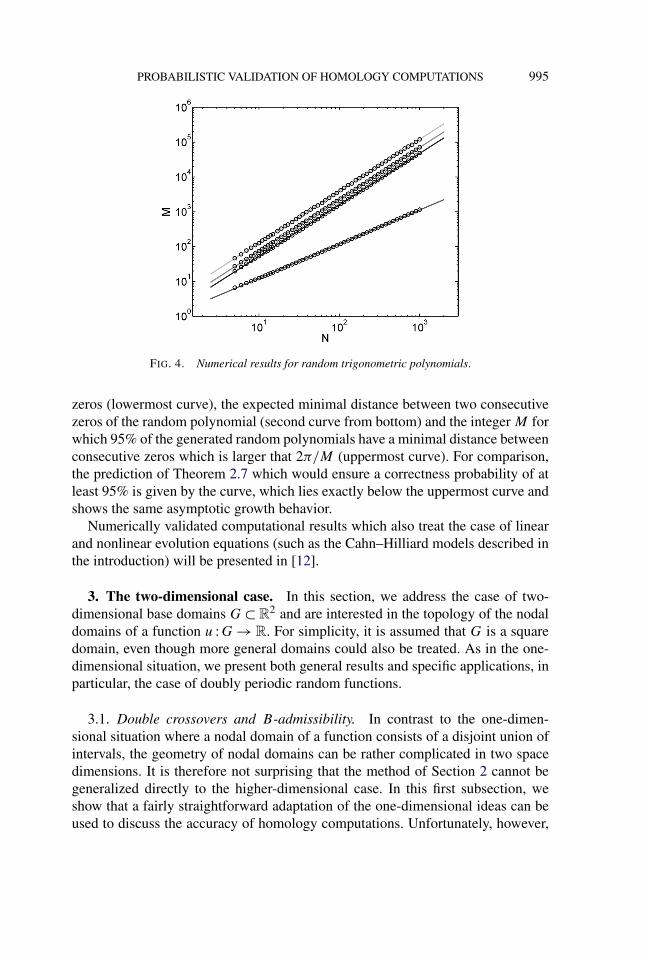
We conjecture that this proportionality is the correct asymptotic result, as is sup-ported by the numerical results shown in Figure 4. For various values of N be-tween 5 and 1000, we computed three different quantities: the expected number of


FIG. 4. Numerical results for random trigonometric polynomials.

zeros (lowermost curve), the expected minimal distance between two consecutivezeros of the random polynomial (second curve from bottom) and the integer M forwhich 95% of the generated random polynomials have a minimal distance betweenconsecutive zeros which is larger that 2π/M (uppermost curve). For comparison,the prediction of Theorem 2.7 which would ensure a correctness probability of atleast 95% is given by the curve, which lies exactly below the uppermost curve andshows the same asymptotic growth behavior.

Numerically validated computational results which also treat the case of linearand nonlinear evolution equations (such as the Cahn–Hilliard models described inthe introduction) will be presented in [12].

3. The two-dimensional case. In this section, we address the case of two-dimensional base domains G ⊂ R

2 and are interested in the topology of the nodaldomains of a function u :G → R. For simplicity, it is assumed that G is a squaredomain, even though more general domains could also be treated. As in the one-dimensional situation, we present both general results and specific applications, inparticular, the case of doubly periodic random functions.

3.1. Double crossovers and B-admissibility. In contrast to the one-dimen-sional situation where a nodal domain of a function consists of a disjoint union ofintervals, the geometry of nodal domains can be rather complicated in two spacedimensions. It is therefore not surprising that the method of Section 2 cannot begeneralized directly to the higher-dimensional case. In this first subsection, weshow that a fairly straightforward adaptation of the one-dimensional ideas can beused to discuss the accuracy of homology computations. Unfortunately, however,


FIG. 5. Examples of problem situations in two dimensions. In each of the three columns, the func-tion values at the grid points shown have identical sign configurations, but the underlying topologyof the nodal domains differs. The nodal lines are shown as solid black lines.

this approach alone will provide suboptimal results and must therefore be extendedsignificantly in the following subsection.

In the one-dimensional situation, the basic ingredients of our approach can besummarized as follows. After recognizing the fundamental obstruction to a validhomology computation as the occurrence of two zeros in an interval betweengridpoints, this obstruction was reformulated in terms of the concept of a doublecrossover. The latter is a specific function value sign pattern that can be observedat the endpoints and midpoint of a given interval J . Moreover, by excluding thissign pattern from all dyadic subintervals of J , we were able to introduce the notionof admissibility of J . Admissibility guarantees that the topological information forthe nodal domains in J can be determined from the function values of the givenfunction at the endpoints of J . If the function values at the endpoints have the samesign, then the function has no zero in J ; if the signs differ, then the function hasexactly one zero in J .

Based on the above discussion, our goal is the identification of certain sign pat-terns of function values that could indicate mistakes in the homology computation.As the fundamental building block, we consider a square with side length δ and,analogously to the one-dimensional case, we consider the function values of theunderlying function u at the corners as well as at the midpoints of the sides and atthe center of the square. This will easily enable us to consider dyadic subsquaresas before.

Some representative examples of problematic sign patterns are shown in Fig-ure 5. Within each column, the two examples exhibit the same sign pattern, but theunderlying topology of the nodal domains differs. The examples in the first twocolumns are, in some sense, reminiscent of the one-dimensional situation since in


FIG. 6. For the notion of B-admissibility, the seven sign configurations shown above are forbidden.Each image corresponds to two sign patterns: one in which the dark points correspond to positivefunction values and the light points correspond to negative ones, and one for the opposite situation.

each of these cases, we can find a double crossover on at least one vertical or hor-izontal line of grid points. This is not true for the examples in the last column ofFigure 5. Here, there are no double crossovers on vertical or horizontal lines, yetthe underlying topology still differs. On the level of the function values of u, thisis due to the fact that, at the corners, the signs alternate. In other words, there aretwo double crossovers around the perimeter of the square. Altogether, we see thateach of the sign configurations shown in Figure 5 contains one of the seven signpatterns depicted in Figure 6.

It turns out that excluding the patterns in Figure 6 is sufficient to extend thegeneral procedure of Section 2. For this, we need the following definitions.

DEFINITION 3.1 (Dyadic subsquares). Let J := [α,α + δ] × [β,β + δ] ⊂ R2

and denote the dyadic points in the interval [0, δ] in the sense of Definition 2.2,by dn,k . Then the dyadic points in the square J are the points

dn,k,� = (α + dn,k, β + dn,�) ∈ R2 for all k, � = 0, . . . ,2n and n ∈ N0.

The dyadic subsquares of J are the squares dn,k,� + [0, δ/2n]2 for all k, � =0, . . . ,2n − 1 and n ∈ N0.

DEFINITION 3.2 (B-admissibility). Let u :G → R denote an arbitrary func-tion and let J ⊂ G denote a square, as in Definition 3.1. Then J is calledB-admissible for u, if none of its dyadic subsquares contain any of the functionvalue sign configurations shown in Figure 6.

Using the concept of B-admissibility, one can validate homology more or lessanalogously to the one-dimensional case. To demonstrate this, consider Figure 7.If we assume that a given square J of side length δ > 0 (shown in pink) isB-admissible for u, then the figure shows all possible function value sign con-figurations which can be observed at the dyadic points d1,k,�, where k, � = 0,1,2,


FIG. 7. Possible sign patterns for the function values of u at the dyadic points d1,k,�, wherek, � = 0,1,2, if the underlying square is B-admissible. In addition to the patterns shown, all signpatterns which can be obtained by applying an element of the symmetry group of the square can alsooccur, resulting in a total of 66 possible patterns.

up to symmetry actions of the square. These configurations are grouped accordingto the sign configurations at the corners of the square. We now make two importantobservations:

• if all function values of u at the four corners of J have the same sign, thenall function values at the nine depicted dyadic points must necessarily have thesame sign;

• if both signs can be observed at the corners of J , then there are exactly two sidesof the square with contain both positive and negative function values.

The first observation is reminiscent of Lemma 2.3. It shows that if J is B-admis-sible for u and u is positive at the corners of J , then u cannot take negative functionvalues on J . Thus the first observation can be used to identify subsets of one or theother nodal domain. In combination with the second observation, it therefore seemsplausible to expect that the nodal line in a B-admissible square can be pinneddown. In fact, under suitable nondegeneracy assumptions on u, it is possible toprove the following result.

PROPOSITION 3.3. Let G ⊂ R2 denote a square, let u :G → R be C2 such

that 0 is not a critical value of u and let J ⊂ G be a B-admissible square for u.Then the following hold.

(a) If u is strictly positive at the corners of J , then u is strictly positive on J .Similarly, if u is strictly negative at the corners of J , then u is strictly negativeon J .

(b) If u takes both positive and negative function values at the corners of J ,then the nodal line of u in J is a simple smooth curve which connects one sideof J with another side of J .


Now, assume the situation of Definition 1.1 with a positive integer M . Ifall M2 subsquares which are generated by adjacent gridpoints of the equidistantM-discretization of G are B-admissible for u, then we have

H∗(N±) ∼= H∗(Q±M),

that is, the homologies of the nodal domains N± and of their cubical approxima-tions Q±

M coincide.

The proof of the above result can easily be formulated using ideas similar tothose for the one-dimensional case and is therefore omitted.

At first glance, Proposition 3.3 is exactly the validation criterion which allowsus to consider the two-dimensional random field case. It is, in fact, possible toproceed as in Section 2 and formulate a probabilistic estimate based on the aboveproposition. Unfortunately, the resulting theorem provides highly suboptimal prob-ability estimates. This suboptimality stems from the fact that the three-point signconfigurations in Figure 6 are not sufficiently unlikely. It turns out that in manyapplications, each of these configurations has probability of order O(δ3), whereδ denotes the side length of the square J . On the other hand, the four-point con-figuration in Figure 6 has probability of order O(δ4). Together, the probability forB-admissibility is of order O(δ3). For the homology validation, we must ensurethat each of the M2 subsquares of G are B-admissible and that δ ∼ 1/M . Thisfinally gives a probability estimate of order O(1/M), in contrast to the O(1/M2)

estimate in one dimension.

3.2. Excluded sign patterns and I -admissibility. The discussion of the lastparagraph indicates two things. On one hand, one has to avoid the one-dimensionaldouble crossover concept in higher dimensions since its occurrence is too likely.On the other hand, the four-point configuration of Figure 6 does exhibit the correctprobability estimate. If we were able to define a notion of admissibility which hasprobability of order O(δ4), then the resulting homology validation result wouldexhibit the desired quadratic order in M .

As a first step toward a suitable admissibility condition, we return to the four-point configuration of Figure 6. It was mentioned above that in many applications,the probability of this sign pattern turns out to be of order O(δ4)—one wouldexpect that nondegenerate affine transformations of this pattern are similarly rare.This leads naturally to the following notion.

DEFINITION 3.4 (I4-admissibility). Let u :G → R and J = [α,α + δ] ×[β,β + δ] ⊂ G. Then J is called I4-admissible for u if it does not contain anyof the function value sign configurations shown in Figure 8.

We are still interested in a recursive approach to homology validation, as de-scribed in Sections 2 and 3.1. It is therefore natural to determine which of the


FIG. 8. For the notion of I4-admissibility, the sixteen sign configurations shown above are forbid-den. As in Figure 6, each image corresponds to two sign patterns.

512 sign patterns on the dyadic points d1,k,�, where k, � = 0,1,2, can occur if theunderlying square is I4-admissible. An exhaustive search shows that only 92 pat-terns remain possible. Up to symmetry actions of the square, these configurationsare shown in Figure 9.

In contrast to the situation described in Section 3.1, not all patterns that are pos-sible under I4-admissibility permit homology validation. The prime example canbe seen in the first row of Figure 9. Even though the signs at the corners of thesquare are all the same, after one level of refinement, the opposite sign appears atthe center of the square. This example shows that the concept of I4-admissibilityalone cannot be used for homology validation, that is, we must exclude more sub-configurations. At the same time, we must ensure that the probability estimatesfor the additionally excluded configurations are sufficiently small. As we will seelater, it can be shown that in the context of random periodic functions, the lastsign configuration in the first row of Figure 9 exhibits an O(δ4)-bound. In fact, weneed not consider the full nine-point pattern, but can rather consider the five-pointsubpattern shown in Figure 10. This leads to the following definition.

DEFINITION 3.5 (I5-admissibility). Let u :G → R and J = [α,α + δ] ×[β,β + δ] ⊂ G. Then J is called I5-admissible for u if it does not contain thefunction value sign configuration shown in Figure 10.


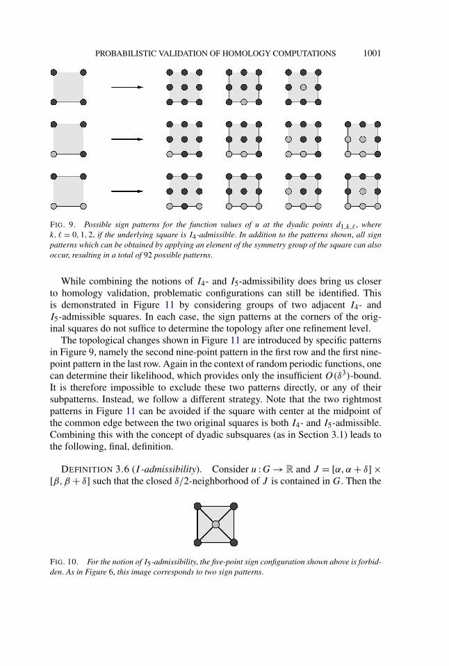
FIG. 9. Possible sign patterns for the function values of u at the dyadic points d1,k,�, wherek, � = 0,1,2, if the underlying square is I4-admissible. In addition to the patterns shown, all signpatterns which can be obtained by applying an element of the symmetry group of the square can alsooccur, resulting in a total of 92 possible patterns.

While combining the notions of I4- and I5-admissibility does bring us closerto homology validation, problematic configurations can still be identified. Thisis demonstrated in Figure 11 by considering groups of two adjacent I4- andI5-admissible squares. In each case, the sign patterns at the corners of the orig-inal squares do not suffice to determine the topology after one refinement level.

The topological changes shown in Figure 11 are introduced by specific patternsin Figure 9, namely the second nine-point pattern in the first row and the first nine-point pattern in the last row. Again in the context of random periodic functions, onecan determine their likelihood, which provides only the insufficient O(δ3)-bound.It is therefore impossible to exclude these two patterns directly, or any of theirsubpatterns. Instead, we follow a different strategy. Note that the two rightmostpatterns in Figure 11 can be avoided if the square with center at the midpoint ofthe common edge between the two original squares is both I4- and I5-admissible.Combining this with the concept of dyadic subsquares (as in Section 3.1) leads tothe following, final, definition.

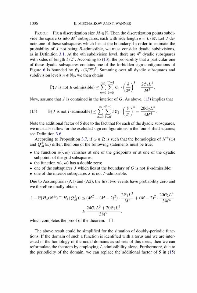
DEFINITION 3.6 (I -admissibility). Consider u :G → R and J = [α,α + δ] ×[β,β + δ] such that the closed δ/2-neighborhood of J is contained in G. Then the

FIG. 10. For the notion of I5-admissibility, the five-point sign configuration shown above is forbid-den. As in Figure 6, this image corresponds to two sign patterns.


FIG. 11. Sample configurations which cannot be detected by using both I4- and I5-admissibility,but which exhibit different topological properties.

square J is called I -admissible for u if for every dyadic subsquare J ∗ of J withside length δ∗ = δ/2n, n ∈ N0, the following five squares are both I4-admissibleand I5-admissible for u:

• the dyadic subsquare J ∗ itself;• the four shifted squares which are obtained by translating J ∗ horizontally or

vertically by δ∗/2 in either direction, as shown in Figure 12.

As mentioned before, it will be shown later that in many situations, it is possibleto derive an O(δ4)-bound for I -admissibility. Note, however, that this improvedbound comes at an additional cost. The notion of I -admissibility is not determinedsolely from the function values of u at the dyadic points in J . Rather, one mustalso include knowledge from certain dyadic points in neighboring squares and this

FIG. 12. For the notion of I -admissibility of a square J , we require that every dyadic subsquare J ∗(shown with shaded background) of J , as well as the four shifted versions of J ∗ shown on the right,are both I4- and I5-admissible. In the figure, the location of the shifted squares is indicated by thefive-point configuration of Figure 10. Nevertheless, all configurations in Figure 8 must be excludedfrom the five indicated squares.


renders I -admissibility impractical at the boundary of G. In order to resolve thisfinal issue, we must combine both B- and I -admissibility in a suitable way. Thisis presented in the next subsection.

3.3. A criterion for homology validation. In the current subsection, the no-tions of B- and I -admissibility are combined to formulate and prove a homologyvalidation criterion in two space dimensions which is amenable to a probabilistictreatment.

While Theorem 1.2 provides a criterion under which it can be guaranteed thatfor sufficiently large M , the homology of the nodal domains agrees with that ofthe cubical approximation, it does not provide insight into how we would deter-mine a minimum value of M . For this, we must consider the notions of B- andI -admissibility.

PROPOSITION 3.7 (Validation criterion). Let G ⊂ R2 denote a square domain

with sides parallel to the coordinate axes and let u :G → R be a twice continu-ously differentiable function for which 0 is a regular value. Let N± denote thenodal domains of u and let Q±

M denote their cubical approximations (as in De-finition 1.1) for some fixed M ∈ N. In addition, suppose that for each of the M2

closed subsquares J formed by adjacent gridpoints in G, u is nonzero at all dyadicsubpoints, and that one of the following holds:

(a) if the square J lies at the boundary of G, then J is B-admissible for u;(b) if the square J lies in the interior of G, then J is I -admissible for u.

We then have

H∗(N±) ∼= H∗(Q±M),

that is, the homologies of the nodal domains and of their cubical approximationscoincide.

PROOF. Let M be fixed as in the formulation of the proposition. In view ofTheorem 1.2, it suffices to show that for all values of n ∈ N, the homologies ofQ±

M·2n and Q±M coincide since then we need only choose n sufficiently large for the

lemma to hold. In order to establish this invariance of the homologies inductively,we only consider the homologies of Q±

2M and Q±M . Subsequent inductive steps can

be carried out completely analogously.Now consider, without loss of generality, a connected component K of the

set Q+M . We can associate with K a collection of positive grid points P in the un-

derlying discretization of G, that is, grid points at which the function u takes posi-tive function values. We must show that the insertion of intermediate grid points inthe underlying grid does not change the topology of the component K in the fol-lowing sense: The corresponding component in Q+

2M has not merged with anothercomponent and the number of holes in K has remained constant.


FIG. 13. Possible sign patterns for the function values of u at the dyadic points d1,k,�, wherek, � = 0,1,2, if the underlying square is I -admissible. In addition to the patterns shown, all signpatterns which can be obtained by applying an element of the symmetry group of the square can alsooccur, resulting in a total of 90 possible patterns. However, the two configurations with patternedbackgrounds can only occur in certain situations which are described in more detail in Figure 14.

In order to perform the step from the given discretization of size M to the one ofsize 2M , we must establish which nine-point sign configurations are possible forevery given four-point sign configuration at the corners of a discretization square.For the concept of B-admissibility, this has already been accomplished in Figure 7.The resulting patterns immediately show that for a B-admissible square, passingfrom M to 2M cannot change the topological properties since no new connec-tions are formed and positive/negative grid points are only introduced adjacent topositive/negative components.

As for the concept of I -admissibility, we must be more careful. In Figure 13, wecollect all possible nine-point sign configurations which could be observed at thenext refinement level. With the exception of the two configurations with patternedbackgrounds, the same comments as in the last paragraph apply to these patternsand they therefore cannot introduce a change in topology.

Now, consider the two remaining nine-point configurations in Figure 13, thatis, the configurations with patterned backgrounds. Recall that our definition ofI -admissibility includes information about neighboring squares and this impliesthat these two configurations can only occur if at the edge of the square with thenewly generated double crossover, the adjacent square exhibits the specific signpattern shown in Figure 14. Thus the newly created double crossovers can onlyoccur at the boundary of the component K and if they appear, they do not createany new connections or introduce any change in topology. This fact also impliesthat in the interior of K , no negative gridpoints can be introduced. In addition, notethat if the adjacent square is, in fact, a B-admissible square, then the two patternedconfigurations cannot occur at all due to the generation of a double crossover.


FIG. 14. The two configurations in Figure 13 with patterned backgrounds can only occur if theneighboring square exhibits a specific sign configuration. For the pattern in the first row of Figure 13,this is shown in the left-hand diagram; for the configuration in the third row see the right-handdiagram.

These facts imply that the topology of the component K will not be changed bypassing from Q+

M to Q+2M and the proof of the proposition is complete. �

We are finally in a position to present an abstract version of a probabilistichomology validation result for two-dimensional random fields u on a square do-main G ⊂ R

2.

THEOREM 3.8 (Abstract 2D estimate). Consider a probability space (�,F ,

P) and the square domain G = [0,L]2 ⊂ R2. Let u :G× � → R denote a random

field over (�,F ,P) satisfying Assumptions (A1) and (A2) such that for P-almostall ω ∈ �, the function u(·,ω) :G → R is twice continuously differentiable. Foreach ω ∈ �, denote the nodal domains of u(·,ω) by N±(ω) ⊂ G and denote theircubical approximations (as in Definition 1.1) by Q±

M(ω).For x = (x1, x2) and δ > 0 such that J = [x1, x1 + δ] × [x2, x2 + δ] ⊂ G, con-

sider the following events in F :

(i) let EB(x, δ) denote the set of all ω ∈ � for which u(·,ω) exhibits at leastone of the seven sign patterns in Figure 6 at the nine dyadic points d1,�,m for�,m = 0,1,2;

(ii) let EI (x, δ) denote the set of all ω ∈ � for which u(·,ω) exhibits atleast one of the seventeen sign patterns in Figures 8 and 10 at the nine dyadicpoints d1,�,m for �,m = 0,1,2.

Assume that there exist positive constants C1 and C2 such that

P(EB(x, δ)) ≤ C1 · δ3 and P(EI (x, δ)) ≤ C2 · δ4(13)

for all x ∈ G and δ > 0 for which J lies in G.Then for every discretization size M , the probability that the homologies

of N±(ω) and Q±M(ω) coincide satisfies

P{H∗(N±) ∼= H∗(Q±M)} ≥ 1 − 24C1L

3 + 20C2L4

3M2 .(14)


PROOF. Fix a discretization size M ∈ N. Then the discretization points subdi-vide the square G into M2 subsquares, each with side length δ = L/M . Let J de-note one of these subsquares which lies at the boundary. In order to estimate theprobability of J not being B-admissible, we must consider dyadic subdivisions,as in Definition 3.1. At the nth subdivision level, there are 4n dyadic subsquareswith sides of length δ/2n. According to (13), the probability that a particular oneof these dyadic subsquares contains one of the forbidden sign configurations ofFigure 6 is bounded by C1 · (δ/2n)3. Summing over all dyadic subsquares andsubdivision levels n ∈ N0, we then obtain

P{J is not B-admissible} ≤∞∑

n=0

4n−1∑k=0

C1 ·(

δ

2n

)3

= 2C1L3

M3 .

Now, assume that J is contained in the interior of G. As above, (13) implies that

P{J is not I -admissible} ≤∞∑

n=0

4n−1∑k=0

5C2 ·(

δ

2n

)4

= 20C2L4

3M4 .(15)

Note the additional factor of 5 due to the fact that for each of the dyadic subsquares,we must also allow for the excluded sign configurations in the four shifted squares;see Definition 3.6.

According to Proposition 3.7, if ω ∈ � is such that the homologies of N±(ω)

and Q±M(ω) differ, then one of the following statements must be true:

• the function u(·,ω) vanishes at one of the gridpoints or at one of the dyadicsubpoints of the grid subsquares;

• the function u(·,ω) has a double zero;• one of the subsquares J which lies at the boundary of G is not B-admissible;• one of the interior subsquares J is not I -admissible.

Due to Assumptions (A1) and (A2), the first two events have probability zero andwe therefore finally obtain

1 − P{H∗(N±) ∼= H∗(Q±M)} ≤ (

M2 − (M − 2)2) · 2C1L3

M3 + (M − 2)2 · 20C2L4

3M4

≤ 24C1L3 + 20C2L

4

3M2 ,

which completes the proof of the theorem. �

The above result could be simplified for the situation of doubly-periodic func-tions. If the domain of such a function is identified with a torus and we are inter-ested in the homology of the nodal domains as subsets of this torus, then we canreformulate the theorem by employing I -admissibility alone. Furthermore, due tothe periodicity of the domain, we can replace the additional factor of 5 in (15)


by 3 since it now suffices to check each square, as well as its down-shift and itsright-shift. Thus for doubly periodic functions, the final probability bound reads

P{H∗(N±) ∼= H∗(Q±M)} ≥ 1 − 4C2L

4

M2 ,

where C2 is as in (13). Finally, as will be demonstrated in the next subsection, thebounds in (13) are optimal for doubly periodic random functions.

3.4. Random periodic functions. As in the one-dimensional case, we closethis section by providing explicit results for the important special case of doublyperiodic functions, that is, for classical random Fourier series.

ASSUMPTION 3.9. We consider random Fourier series on G = [0,L]2 of theform

u(x,ω) =∞∑

k,�=0

ak,� ·(gk,�,1(ω) cos

2πkx1

Lcos

2π�x2

L

+ gk,�,2(ω) cos2πkx1

Lsin

2π�x2

L(16)

+ gk,�,3(ω) sin2πkx1

Lcos

2π�x2

L

+ gk,�,4(ω) sin2πkx1

Lsin

2π�x2

L

)which satisfy the following:

(a) The random variables gk,�,m in (16) are defined over a probability space(�,F ,P) and are independent and normally distributed with mean 0 and vari-ance 1.

(b) there exist positive k1, �1 ∈ N and nonnegative k2, �2 ∈ N0 which satisfyk1 = k2 and �1 = �2, as well as k2

1 + �21 = k2

2 + �22, such that both ak1,�1 and ak2,�2

are nonzero. In addition, suppose that∞∑

k,�=0

(k6 + �6)a2k,� < ∞.

As before, the summability condition in Assumption 3.9(b) is related to smooth-ness properties of the random field u. In fact, it guarantees that the function u(·,ω)

has continuous partial derivatives up to order two for P-almost all ω ∈ �. More-over, if we define

Ap,q =∞∑

k,�=0

k2p�2qa2k,�,(17)


then we can readily show that

E‖Dpx1

Dqx2

u‖2L2(G)

= (2π)2p+2q · L2−2p−2q · Ap,q,

where E denotes the expected value of a random variable over (�,F ,P).As in the one-dimensional case, doubly periodic functions simplify our discus-

sion, in that their spatial covariance function is shift-invariant. More precisely, thespatial covariance function of (16) which is given by

R(x, y) = Eu(x)u(y) =∞∑

k,�=0

a2k,� · cos

2πk(x1 − y1)

L· cos

2π�(x2 − y2)

L.(18)

Adopting this setting, we obtain the following result.

THEOREM 3.10 (Random doubly periodic functions in 2D). Consider therandom Fourier series u defined in (16) and suppose that Assumption 3.9 is sat-isfied. Let M denote an arbitrary positive integer and let Q±

M(ω) denote the cubi-cal approximations of the random nodal domains N±(ω) of u(·,ω) (as in Defini-tion 1.1) which are used for the computation of the homologies of N±(ω). Then theprobability that the homology of the random nodal domains N±(ω) is computedcorrectly with the discretization of size M satisfies

P{H∗(N±) ∼= H∗(Q±M)} ≥ 1 − 1067π2

18M2 · (A2,0 + A1,1 + A0,2)2

A1/20,0 A

1/20,1 A

1/21,0 A

1/21,1

(19)

+ O

(1

M3

),

where Ap,q was defined in (17).

PROOF. According to our assumptions, the random variable u(x, ·) :� → R

is normally distributed with mean 0 and variance∑∞

k,�=0 a2k,� = 0 for each x ∈ G

and this implies (A1). Furthermore, (A2) follows from [1], Theorem 3.2.1. Thusin order to apply Theorem 3.8, we need only verify (13).

As in the proof of Theorem 2.7, we employ Proposition 4.1 with n = 3 orn = 4 to estimate the probability of the various sign patterns, if one considers asquare with side length δ, as in (13). Since this can basically be done as in the one-dimensional case, we have only collected the necessary spectral information for thevarious covariance matrices in Tables 1–6. In each of these tables, the expansionsof the determinant of the covariance matrix C(δ), the expansions of the eigenval-ues and the expansion for the eigenvector corresponding to λ1(δ) are given. Theconstants Rp,q which appear in these formulas arise in the expansion of the spatialcovariance function (18). More precisely, if we set

r(d) = R(y + d, y) =∞∑

k,�=0

a2k,� · cos

2πkd1

L· cos

2π�d2

L,


TABLE 1Covariance matrix spectral information for the first shown sign pattern. For the second pattern, we

must replace R0,� by R�,0

detC(δ) = R0,1(R0,0R0,2 − R20,1)

64· δ6 + O(δ7)

λ1(δ) = R0,0R0,2 − R20,1

96R0,0· δ4 + O(δ5)

λ2(δ) = R0,1

2· δ2 + O(δ3)

λ3(δ) = 3R0,0 + O(δ)

v1(δ) = 1√6

· (1,−2,1)t + O(δ)

TABLE 2Covariance matrix spectral information for the sign pattern shown

detC(δ) = R0,0R0,1R1,0R1,1 · δ8 + O(δ9)

λ1(δ) = R1,1

4· δ4 + O(δ5)

λ2(δ) = 2R0,1R1,0

R0,1 + R0,1 + |R0,1 − R0,1| · δ2 + O(δ3)

λ3(δ) = R0,1 + R0,1 + |R0,1 − R0,1|2

· δ2 + O(δ3)

λ4(δ) = 4R0,0 + O(δ)

v1(δ) = 12 · (1,−1,1,−1)t + O(δ)


detC(δ) = R0,0R0,1R1,0R1,1

256· δ8 + O(δ9)

λ1(δ) = R1,1

64· δ4 + O(δ5)

λ2(δ) = R0,1R1,0

2(R0,1 + R0,1 + |R0,1 − R0,1|) · δ2 + O(δ3)

λ3(δ) = R0,1 + R0,1 + |R0,1 − R0,1|8

· δ2 + O(δ3)

λ4(δ) = 4R0,0 + O(δ)

v1(δ) = 12 · (1,−1,1,−1)t + O(δ)


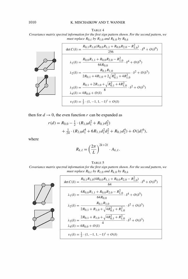
TABLE 4Covariance matrix spectral information for the first sign pattern shown. For the second pattern, we

must replace R0,� by R�,0 and Rk,0 by R0,k

detC(δ) = R0,1R1,0(R0,0R1,1 + R0,0R2,0 − R21,0)

256· δ8 + O(δ9)

λ1(δ) = R0,0R1,1 + R0,0R2,0 − R21,0

64R0,0· δ4 + O(δ5)

λ2(δ) = R0,1R1,0

2R0,1 + 4R1,0 + 2√

R20,1 + 4R2

1,0

· δ2 + O(δ3)

λ3(δ) =R0,1 + 2R1,0 +

√R2

0,1 + 4R21,0

8· δ2 + O(δ3)

λ4(δ) = 4R0,0 + O(δ)

v1(δ) = 12 · (1,−1,1,−1)t + O(δ)

then for d → 0, the even function r can be expanded as

r(d) = R0,0 − 12 · (R1,0d

21 + R0,1d

22 )

+ 124 · (R2,0d

41 + 6R1,1d

21d2

2 + R0,2d42 ) + O(|d|6),

where

Rk,� =(

2π

L

)2k+2�

· Ak,�.

TABLE 5Covariance matrix spectral information for the first sign pattern shown. For the second pattern, we

must replace R0,� by R�,0 and Rk,0 by R0,k

detC(δ) = R0,1R1,0(4R0,0R1,1 + R0,0R2,0 − R21,0)

64· δ8 + O(δ9)

λ1(δ) = 4R0,0R1,1 + R0,0R2,0 − R21,0

64R0,0· δ4 + O(δ5)

λ2(δ) = R0,1R1,0

2R0,1 + R1,0 +√

4R20,1 + R2

1,0

· δ2 + O(δ3)

λ3(δ) =2R0,1 + R1,0 +

√4R2

0,1 + R21,0

4· δ2 + O(δ3)

λ4(δ) = 4R0,0 + O(δ)

v1(δ) = 12 · (1,−1,1,−1)t + O(δ)



R∗ = R0,0(R0,2 + 2R1,1 + R2,0) − (R0,1 + R1,0)2

detC(δ) = R0,1R1,0R1,1R∗64

· δ12 + O(δ13)

λ1(δ) = R∗80R0,0

· δ4 + O(δ5)

λ2(δ) = R1,1

4· δ4 + O(δ5)

λ3(δ) = 2R0,1R1,0

R0,1 + R1,0 + |R0,1 − R1,0| · δ2 + O(δ3)

λ4(δ) = R0,1 + R1,0 + |R0,1 − R1,0|2

· δ2 + O(δ3)

λ5(δ) = 5R0,0 + O(δ)

v1(δ) = 1

2√

5· (1,1,1,1,−4)t + O(δ)

In addition, we can easily verify that all of the leading coefficients in the expan-sions of the tables are nonzero due to Assumption 3.9(b).

By combining the information in Tables 1 and 2 with Proposition 4.1 and thedefinition of EB(x, δ) in (13), we obtain the estimate

P(EB(x, δ)) ≤ 6 · δ3

128π· R0,0R0,2 − R2

0,1

R3/20,0 R

1/20,1

+ 6 · δ3

128π· R0,0R2,0 − R2

1,0

R3/20,0 R

1/21,0

+ 2 · δ4

12π2 · R3/21,1

R1/20,0 R

1/20,1 R

1/21,0

≤ 3δ3

64π· R0,2R

1/21,0 + R2,0R

1/20,1

R1/20,0 R

1/20,1 R

1/21,0

+ δ4

6π2 · R3/21,1

R1/20,0 R

1/20,1 R

1/21,0

= 3π2δ3

8L3 · A0,2A1/21,0 + A2,0A

1/20,1

A1/20,0 A

1/20,1 A

1/21,0

+ 8π2δ4

3L4 · A3/21,1

A1/20,0 A

1/20,1 A

1/21,0

≤ 41π2δ3

12L3 · (A2,0 + A1,1 + A0,2)3/2

A1/20,0 A

1/20,1 A

1/21,0

.

Note that the three terms after the first inequality correspond to the bounds for thetwo patterns in Table 1 and the pattern in Table 2 (in that order); the additionalfactors 6, 6 and 2 correspond to the multiplicities of each pattern. For example, the


first vertical pattern must be tested twice (depending on whether the interior pointis positive or negative) on each of the three vertical lines.

From the above estimate, we can readily see that the first part of (13) is satisfiedwith

C1 = 41π2

12L3 · (A2,0 + A1,1 + A0,2)2

A1/20,0 A

1/20,1 A

1/21,0 A

1/21,1

.

Similarly, by combining the information in Tables 3–6 with Propositions 4.1and 4.2 (for the five-point sign pattern) and recalling the definition of EI (x, δ)

in (13), we obtain the estimate

P(EI (x, δ)) ≤ 8 · δ4

192π2 · R3/21,1

R1/20,0 R

1/20,1 R

1/21,0

+ 8 · δ4

192π2 · (R2,0 + R1,1)3/2

R1/20,0 R

1/20,1 R

1/21,0

+ 8 · δ4

192π2 · (R0,2 + R1,1)3/2

R1/20,0 R

1/20,1 R

1/21,0

+ 4 · δ4

384π2 · (R2,0 + 4R1,1)3/2

R1/20,0 R

1/20,1 R

1/21,0

+ 4 · δ4

384π2 · (R0,2 + 4R1,1)3/2

R1/20,0 R

1/20,1 R

1/21,0

+ 2 · δ4

1024π2 · (R0,2 + 2R1,1 + R2,0)2

R1/20,0 R

1/20,1 R

1/21,0 R

1/21,1

≤ 115δ4

384π2 · (R0,2 + R1,1 + R2,0)2

R1/20,0 R

1/20,1 R

1/21,0 R

1/21,1

,

that is, we can set

C2 = 115π2

24L4 · (A2,0 + A1,1 + A0,2)2

A1/20,0 A

1/20,1 A

1/21,0 A

1/21,1

.

Thus, (13) is also satisfied and Theorem 3.10 follows from our abstract result,Theorem 3.8. �

It is clear from the above proof that the bound in (19) is not optimal. Its formis chosen to point out the essential ingredients, but not to establish the tightest fit.We do believe, however, that it reflects the true situation fairly accurately.

3.5. Random bivariate trigonometric polynomials. As in the one-dimensionalcase, we illustrate our main theorem for random doubly periodic functions usingrandom trigonometric polynomials. For this, let N ≥ 3 denote an arbitrary inte-ger. If, in the situation of Theorem 3.10, we choose the coefficients as ak,� = 1for 1 ≤ k, � ≤ N and ak,� = 0 otherwise, then (16) represents a bivariate random


trigonometric polynomial. Now, let A� be defined as in (17). We can then easilyshow that

(A2,0 + A1,1 + A0,2)2

A1/20,0 A

1/20,1 A

1/21,0 A

1/21,1

= 1

900· (46N2 + 51N − 7)2 ∼ 529

225· N4.

This implies that in order for the homology computation to be accurate with highconfidence, we must choose the discretization size M in such a way that

M ∼ N2 for N → ∞,

in contrast to the one-dimensional case. Numerically validated computational re-sults which provide more insight into the asymptotic behavior of M will be pre-sented in [12].

4. Probabilistic tools. The central probabilistic tools used in the results of theprevious sections are concerned with the asymptotic behavior of sign-distributionprobabilities of parameter-dependent Gaussian random variables. More precisely,let T (δ) = (T1(δ), . . . , Tn(δ))

t ∈ Rn denote a one-parameter family of R

n-valuedrandom Gaussian variables over a probability space (�,F ,P), indexed by δ > 0,and choose a sign sequence (s1, . . . , sn) ∈ {±1}n. We are then interested in theasymptotic behavior of the probability

P(δ) = P{sjTj (δ) ≥ 0 for all j = 1, . . . , n}.(20)

To this end, we derive two results. While the first result establishes the preciseasymptotic behavior of P(δ) as δ → 0, the second result furnishes an upper boundunder considerably weakened hypotheses.

4.1. Precise asymptotics. We begin with a result which establishes the preciseasymptotic behavior of sign-distribution probabilities.

PROPOSITION 4.1. Let (s1, . . . , sn) ∈ {±1}n denote a fixed sign sequence andconsider a one-parameter family T (δ), δ > 0, of R

n-valued random Gaussian vari-ables over a probability space (�,F ,P) which satisfies the following assump-tions:

(i) For each δ > 0, assume that the Gaussian random variable T (δ) hasmean 0 ∈ R

n and a positive-definite covariance matrix C(δ) ∈ Rn×n, whose pos-

itive eigenvalues are given by λ1(δ), . . . , λn(δ). The corresponding orthonormal-ized eigenvectors are denoted by v1(δ), . . . , vn(δ).

(ii) There exists a vector v1 = (v11, . . . , v1n)t ∈ R

n such that v1(δ) → v1 asδ → 0 and sj · v1j > 0 for all j = 1, . . . , n.

(iii) The quotient λ1(δ)/λk(δ) converges to 0 as δ → 0 for all k = 2, . . . , n.


Then the probability P(δ) defined in (20) satisfies

limδ→0

P(δ) ·√

detC(δ)

λ1(δ)n= �(n/2)

2 · πn/2 · (n − 1)! ·∣∣∣∣∣

n∏j=1

v1j

∣∣∣∣∣−1

.(21)

Recall that �(1/2) = π1/2, �(1) = 1 and �(t + 1) = t�(t) for t > 0.

PROOF. Define the diagonal matrix S = (siδij )i,j=1,...,n, where δij denotes theKronecker delta, and let Z+ = {z ∈ R

n : zj ≥ 0 for j = 1, . . . , n}. Finally, let

D(δ) = λ1(δ) · SC(δ)−1S.

Using the density of the Gaussian distribution of T (δ) according to [3], Theo-rem 30.4, which exists since C(δ) is positive-definite, in combination with a simplerescaling, the probability in (20) can be rewritten as

P(δ) = (2π)−n/2√

detC(δ)·∫Z+

e−zt SC(δ)−1Sz/2 dz =√

λ1(δ)n

πn detC(δ)·∫Z+

e−ztD(δ)z dz.

According to our assumptions, the eigenvalues µ1(δ), . . . ,µn(δ) of the ma-trix D(δ) are given by

µ1(δ) = 1 and µk(δ) = λ1(δ)

λk(δ)for k = 2, . . . , n,

with corresponding orthonormalized eigenvectors wk(δ) = Svk(δ) for k = 1, . . . ,

n. Now, let B(δ) denote the orthogonal matrix with columns w1(δ), . . . ,wn(δ) andintroduce the change of variables z = B(δ)ζ . Moreover, let

Z(ζ1, δ) ={(ζ2, . . . , ζn) :

n∑k=1

ζkwk(δ) ∈ Z+}

⊂ Rn−1

and define

I (ζ1, δ) =∫Z(ζ1,δ)

exp

(−

n∑k=2

µk(δ)ζ2k

)d(ζ2, . . . , ζn).

Due to (ii) and the definition of the signs sk , the eigenvector w1(δ) has strictlypositive components for all sufficiently small δ > 0 and therefore the identity

ztD(δ)z =n∑

k=1

µkζ2k

implies that ∫Z+

e−ztD(δ)z dz =∫B(δ)−1Z+

exp

(−

n∑k=1

µkζ2k

)dζ

(22)=

∫ ∞0

I (ζ1, δ)e−ζ 2

1 dζ1.


From the definition of I (ζ1, δ), we can easily deduce that

I (ζ1, δ) = ζ n−11 ·

∫Z(1,δ)

exp

(−ζ 2

1 ·n∑

k=2

µk(δ)η2k

)d(η2, . . . , ηn)

and this representation implies that

I (ζ1, δ) ≤ ζ n−11 · voln−1(Z(1, δ)) for all ζ1 > 0 and δ > 0.(23)

Again, according to (ii), the (n − 1)-dimensional volume of the simplex Z(1, δ)

converges to the (n − 1)-dimensional volume of the simplex

Z = {z ∈ Z+ : (z − Sv1, Sv1) = 0} ⊂ Rn,

which can be computed as

voln−1(Z) = 1

(n − 1)! ·∣∣∣∣∣

n∏j=1

v1j

∣∣∣∣∣−1

.

Now, let ζ1 > 0 be arbitrary, but fixed. Note that since we did not make any as-sumptions about the asymptotic behavior of the eigenvectors w2(δ), . . . ,wn(δ) forδ → 0, the sets Z(1, δ) do not have to converge. Yet, (ii) yields the existence of acompact subset K ⊂ R

n−1 such that Z(1, δ) ⊂ K for all sufficiently small δ > 0.Due to (iii), the integrand in (22) converges to 1 uniformly on K and we thereforehave

limδ→0

I (ζ1, δ) = ζ n−11 · voln−1(Z) for all ζ1 > 0.

Due to (23) and voln−1(Z(1, δ)) → voln−1(Z), we can now apply the dominatedconvergence theorem to pass to the limit δ → 0 in (22), which leads to

limδ→0

∫Z+

e−ztD(δ)z dz = voln−1(Z) ·∫ ∞

0ζ n−1

1 e−ζ 21 dζ1 = voln−1(Z) · �(n/2)

2.

This completes the proof of the proposition. �

The above result is the main probabilistic tool for our one-dimensional resultsin Section 2. In this situation, Proposition 4.1 is used to study random variablesin R

3. We note that for three-dimensional random variables, it is, in fact, possibleto explicitly compute the probability P(δ) for each δ > 0 as a function of theentries in the covariance matrix C(δ). This has been demonstrated in [15] using theinversion formula ([5], Formula (29.3)) and could be used to study the asymptoticbehavior of P(δ) as δ → 0. However, for the results of Section 3, we must alsoconsider higher-dimensional random vectors and the method in [15] no longerapplies.


4.2. Upper bounds. While the above result establishes the precise asymptoticbehavior of the sign-distribution probability P(δ), the necessary assumptions forProposition 4.1 are not satisfied in all instances discussed in Section 3. Yet, in thesecases, it suffices to obtain an upper bound on the probability P(δ). Such an upperbound is the subject of the following result, which can be derived under fairly weakassumptions.

PROPOSITION 4.2. Let (s1, . . . , sn) ∈ {±1}n denote a fixed sign sequence andconsider a one-parameter family T (δ), δ > 0, of R

n-valued random Gaussian vari-ables over a probability space (�,F ,P) which satisfies the following assump-tions:

(i) For each δ > 0, the Gaussian random variable T (δ) has vanishingmean 0 ∈ R

n and a positive-definite covariance matrix C(δ) ∈ Rn×n whose pos-

itive eigenvalues are given by λ1(δ), . . . , λn(δ). Corresponding orthonormalizedeigenvectors are denoted by v1(δ), . . . , vn(δ).

(ii) There exists a vector v1 = (v11, . . . , v1n)t ∈ R

n such that v1(δ) → v1 asδ → 0 and sj · v1j > 0 for all j = 1, . . . , n.

Then the probability P(δ) defined in (20) satisfies

lim supδ→0

P(δ) ·√

detC(δ)

λ1(δ)n≤ �(n/2)

2 · πn/2 · (n − 1)! ·∣∣∣∣∣

n∏j=1

v1j

∣∣∣∣∣−1

.(24)

PROOF. We adopt the notation used in the proof of Proposition 4.1. We thenhave

P(δ) = (2π)−n/2√

detC(δ)·∫Z+

e−zt SC(δ)−1Sz/2 dz

=√

λ1(δ)n

πn detC(δ)·∫ ∞

0I (ζ1, δ)e

−ζ 21 dζ1,

where

I (ζ1, δ) = ζ n−11 ·

∫Z(1,δ)

exp

(−ζ 2

1 ·n∑

k=2

µk(δ)η2k

)d(η2, . . . , ηn)

≤ ζ n−11 · voln−1(Z(1, δ)).

It was shown in the proof of Proposition 4.1 that voln−1(Z(1, δ)) → voln−1(Z) isa consequence of (ii), and this immediately implies (24). �

Note that Proposition 4.2 does not require any assumption of the eigen-value λ1(δ). In particular, λ1(δ) need not be the smallest positive eigenvalue


of C(δ), in contrast to Proposition 4.1. We also note that we could easily mod-ify the above result to yield lower bounds for the asymptotic behavior of P(δ).Since these are not needed for our applications, we refrain from formulating themhere.

Acknowledgment. The authors would like to thank the anonymous refereefor his careful reading of the manuscript and useful suggestions.

REFERENCES

[1] ADLER, R. J. (1981). The Geometry of Random Fields. Wiley, Chichester. MR0611857[2] ADLER, R. J. and TAYLOR, J. E. (2007). Random Fields and Geometry. Springer, New York.[3] BAUER, H. (1996). Probability Theory. de Gruyter, Berlin. MR1385460[4] BHARUCHA-REID, A. T. and SAMBANDHAM, M. (1986). Random Polynomials. Academic

Press, Orlando. MR0856019[5] BILLINGSLEY, P. (1995). Probability and Measure, 3rd. ed. Wiley, New York. MR1324786[6] BLÖMKER, D., MAIER-PAAPE, S. and WANNER, T. (2001). Spinodal decomposition for the

Cahn–Hilliard–Cook equation. Comm. Math. Phys. 223 553–582. MR1866167[7] BLÖMKER, D., MAIER-PAAPE, S. and WANNER, T. (2007). Second phase spinodal decom-

position for the Cahn–Hilliard–Cook equation. Trans. Amer. Math. Soc. To appear.[8] CAHN, J. W. (1968). Spinodal decomposition. Trans. Metallurgical Society of AIME 242

166–180.[9] CAHN, J. W. and HILLIARD, J. E. (1958). Free energy of a nonuniform system I. Interfacial

free energy. J. Chem. Phys. 28 258–267.[10] CARLSSON, G. and DE SILVA, V. (2003). Topological approximation by small simplicial com-

plexes. Preprint.[11] DAY, S., KALIES, W. D., MISCHAIKOW, K. and WANNER, T. (2007). Probabilistic and nu-

merical validation of homology computations for nodal domains. Submitted for publica-tion.

[12] DAY, S., KALIES, W. D. and WANNER, T. (2007). Homology computations of nodal domains:Accuracy estimates and validation. In preparation.

[13] DE SILVA, V. and CARLSSON, G. (2004). Topological estimation using witness complexes. InEurographics Symposium on Point-Based Graphics (M. Alexa and S. Rusinkiewicz, eds.)The Eurographics Association.

[14] DONOHO, D. L. and GRIMES, C. (2003). Hessian eigenmaps: Locally linear embedding tech-niques for high-dimensional data. Proceedings of the National Academy of Science 1005591–5596. MR1981019

[15] DUNNAGE, J. E. A. (1966). The number of real zeros of a random trigonometric polynomial.Proc. London Math. Soc. 16 53–84. MR0192532

[16] EDELMAN, A. and KOSTLAN, E. (1995). How many zeros of a random polynomial are real?Bull. Amer. Math. Soc. 32 1–37. MR1290398

[17] FARAHMAND, K. (1998). Topics in Random Polynomials. Longman, Harlow. MR1679392[18] GAMEIRO, M., MISCHAIKOW, K. and KALIES, W. (2004). Topological characterization of

spatial-temporal chaos. Phys. Rev. E 70 035203. MR2129999[19] GAMEIRO, M., MISCHAIKOW, K. and WANNER, T. (2005). Evolution of pattern complexity

in the Cahn–Hilliard theory of phase separation. Acta Materialia 53 693–704.[20] HYDE, J. M., MILLER, M. K., HETHERINGTON, M. G., CEREZO, A., SMITH, G. D. W. and

ELLIOTT, C. M. (1995). Spinodal decomposition in Fe-Cr alloys: Experimental study atthe atomic level and comparison with computer models—II. Development of domain sizeand composition amplitude. Acta Metallurgica et Materialia 43 3403–3413.

http://www.ams.org/mathscinet-getitem?mr=0611857











[21] HYDE, J. M., MILLER, M. K., HETHERINGTON, M. G., CEREZO, A., SMITH, G. D. W. andELLIOTT C. M. (1995). Spinodal decomposition in Fe-Cr alloys: Experimental study atthe atomic level and comparison with computer models—III. Development of morphol-ogy. Acta Metallurgica et Materialia 43 3415–3426.

[22] KAHANE, J.-P. (1985). Some Random Series of Functions, 2nd ed. Cambridge Univ. Press.MR0833073

[23] KRISHAN, K., GAMEIRO, M., MISCHAIKOW, K. and SCHATZ, M. F. (2005). Homologicalcharacterization of spiral defect chaos in Rayleigh–Benard convection. Preprint.

[24] MILLER, M. K., HYDE, J. M., HETHERINGTON, M. G., CEREZO, A., SMITH, G. D. W. andELLIOTT, C. M. (1995). Spinodal decomposition in Fe-Cr alloys: Experimental study atthe atomic level and comparison with computer models—I. Introduction and methodol-ogy. Acta Metallurgica et Materialia 43 3385–3401.

[25] NIYOGI, P., SMALE, S. and WEINBERGER, S. (2007). Finding the homology of submanifoldswith high confidence from random samples. Discrete and Computational Geometry. Toappear.

[26] ROWEIS, S. T. and SAUL, L. K. (2000). Nonlinear dimensionality reduction by locally linearembedding. Science 290 2323–2326.

[27] SIDOROV, N., LOGINOV, B., SINITSYN, A. and FALALEEV, M. (2002). Lyapunov–SchmidtMethods in Nonlinear Analysis and Applications. Kluwer, Dordrecht. MR1959647

[28] TENENBAUM, J. B., DE SILVA, V. and LANGFORD, J. C. (2000). A global geometric frame-work for nonlinear dimensionality reduction. Science 290 2319–2323.

[29] VAINBERG, M. M. and TRENOGIN, V. A. (1974). Theory of Branching of Solutions of Non-Linear Equations. Noordhoff International Publishing, Leyden.

[30] WANNER, T. (2004). Maximum norms of random sums and transient pattern formation. Trans.Amer. Math. Soc. 356 2251–2279. MR2048517

DEPARTMENT OF MATHEMATICS

RUTGERS UNIVERSITY

PISCATAWAY, NEW JERSEY 08854USAE-MAIL: [email protected]

DEPARTMENT OF MATHEMATICAL SCIENCES

GEORGE MASON UNIVERSITY

FAIRFAX, VIRGINIA 22030USAE-MAIL: [email protected]




mailto:[email protected]

mailto:[email protected]

probabilistic validation of homology computations for...

Documents