PROBING THE STATISTICAL STRUCTURE OF

TURBULENCE WITH MEASUREMENTS OF TRACER

PARTICLE TRACKS

A Dissertation

Presented to the Faculty of the Graduate School

of Cornell University

in Partial Fulfillment of the Requirements for the Degree of

Doctor of Philosophy

by

Nicholas Testroet Ouellette

May 2006

c© 2006 Nicholas Testroet Ouellette

ALL RIGHTS RESERVED

PROBING THE STATISTICAL STRUCTURE OF TURBULENCE WITH

MEASUREMENTS OF TRACER PARTICLE TRACKS

Nicholas Testroet Ouellette, Ph.D.

Cornell University 2006

This thesis reports measurements of the statistics of passive Lagrangian tracer

particles in an intensely turbulent laboratory water flow. The tracers are imaged

with three high-speed CMOS cameras and their trajectories are reconstructed using

specialized particle tracking algorithms. Various tracking algorithms were studied

quantitatively to determine the algorithm used in this work.

The scaling behavior of the Lagrangian structure functions is investigated as

a function of structure function order, and is found to deviate strongly from the

Kolmogorov (1941a) prediction. The second order Lagrangian structure function

is considered in detail, and its scaling constant C0, an essential parameter in tur-

bulence models, is measured independently from the structure function and the

Lagrangian velocity spectrum. These measurements of C0 show strong anisotropy.

These results are confirmed by measurements of the spatial dispersion of single

tracer particles. In addition, the first measurement of the multifractal dimension

spectrum of Lagrangian turbulence is reported.

The relative motion of multiple tracer particles is also measured. Turbulent

relative dispersion, the growth of the separation of a pair of tracers, is measured

and found to be in excellent agreement with the results of Batchelor (1950), with

no observed Richardson-Obukhov scaling. Other proposed models of turbulent

relative dispersion are also investigated in detail. A coarse-grained model of the

velocity gradient tensor based on clusters of four tracers, known as tetrads, is also

investigated, as well as the statistics of the tetrad shape changes.

BIOGRAPHICAL SKETCH

Nicholas Testroet Ouellette was born on April 5, 1980 in Albany, New York,

the only child of Michael and Helen. After moving from nearby Schenectady

to Chicago and then to Amherst, Massachusetts, Nick and his family settled in

Cambridge, Massachusetts in 1990. There, Nick attended Buckingham Browne &

Nichols School, graduating in 1998. He attended Swarthmore College for his un-

dergraduate degree and graduated in 2002 with high honors in both Physics and

Computer Science. At Swarthmore, he wrote his honors thesis under the guidance

of Professor John Boccio, studying quantum computation. In 2002, he began his

graduate work at Cornell, where he has worked with Professor Eberhard Boden-

schatz. Nick has wholeheartedly enjoyed his time in Ithaca, which was highlighted

by his marriage to Lisa Larrimore on August 21, 2004. In his spare time, Nick

enjoys rock climbing, Mahler symphonies, gourmet food, and wine tasting, and he

spends altogether too much time obsessing over the Boston Red Sox.

iii

To my grandparents,

Mike and Jean Ouellette and Frank and Dorothy Testroet.

iv

ACKNOWLEDGEMENTS

Science is never done in a vacuum, and the work presented here is no exception.

I am incredibly grateful for the support of my advisor, Eberhard Bodenschatz,

whose sheer excitement for science is contagious. He has always helped me un-

derstand how our work fits in with that of the broader scientific community. By

challenging me to think for myself and allowing me to design my own experiments,

he has helped me to become a more self-reliant scientist. I have very much appre-

ciated the opportunity to attend many conferences and meetings; discussing my

work with other scientists has been an important part of my graduate career. I

will always remember Eberhard’s mantra of being proud of my work.

I also owe a huge debt of gratitude to Haitao Xu, without whom my thesis

work would never have been finished. Haitao always seemed to know a way to fix

whatever problems cropped up in the lab, and he taught me everything I know

about error analysis. His independent analysis of our data was invaluable for much

of the work in this thesis. Haitao has also graciously taught me diplomacy with

his patient comments on seemingly endless paper drafts.

I have been lucky to be a part of a dynamic and supportive group of collabora-

tors here at Cornell. Many thanks to the rest of the Cornell Lagrangian turbulence

group: Nicolas Mordant and Alice Crawford, for passing on a (more or less) re-

liable experiment and their experience in dealing with the kind of mishaps that

are inevitable in a lab with large quantities of water; Mickael Bourgoin, for the

excellent control systems on the new experiment and for being my translator in

Nice; Jacob Berg, for being a source of constant amusement; Sathya Ayyalaso-

mayajula and Armann Gylfason, for putting up with all our noisy computers when

we moved into their lab this past year; Andrea Lamorgese, for patiently listening

v

to our experimental woes throughout endless meetings; Lance Collins and Zellman

Warhaft, for sharing their wisdom and experience; and, more recently, Kelken

Chang, Matthias Kinzel, Laurent Mydlarski, Holger Nobach, and Dario Vincenzi.

Thanks also to the rest of the Bodenschatz group, who have helped create a great

working environment: Albert Bae, Carsten Beta, Will Brunner, Stefan and Gisa

Luther, Angela Meister, Jon McCoy, Katharina Schneider, Amgad Squires, and

Danica Wyatt. Thanks especially to Jon for reading all my paper drafts without

complaining and for patiently explaining things to me whenever I had a math

question.

I have also benefited a great deal from the kindness of other scientists in the

field who have shared their insight and time with me. Many thanks to Guido

Boffetta, Antonio Celani, Laurent Chevillard, Bob Ecke, Grisha Falkovich, Julian

Hunt, Jakob Mann, Søren Ott, Alain Pumir, Brian Sawford, Jorg Schumacher,

Raymond Shaw, Willem van de Water, Richard Wiener, P. K. Yeung, and former

Bodenschatz group members Karen Daniels and Greg Voth.

I would never had made it this far without the love and support of my family.

Many thanks to my parents, Michael and Helen, for believing in me and always

being willing to listen to long-winded descriptions of whatever I’m working on.

And, of course, thanks and love to Lisa, my partner in everything.

Finally, none of this research would have been possible without generous fund-

ing from both the National Science Foundation and the Max Planck Society.

vi

TABLE OF CONTENTS

Biographical Sketch . . . . . . . . . . . . . . . . . . . . . . . . . . . . . . iiiDedication . . . . . . . . . . . . . . . . . . . . . . . . . . . . . . . . . . . ivAcknowledgements . . . . . . . . . . . . . . . . . . . . . . . . . . . . . . vTable of Contents . . . . . . . . . . . . . . . . . . . . . . . . . . . . . . . viiList of Tables . . . . . . . . . . . . . . . . . . . . . . . . . . . . . . . . . ixList of Figures . . . . . . . . . . . . . . . . . . . . . . . . . . . . . . . . . x

1 Introduction 1

2 Theory and Phenomenology 52.1 The Governing Equations of Fluid Dynamics . . . . . . . . . . . . . 52.2 Homogeneous, Isotropic Turbulence and Kolmogorov’s Hypotheses . 112.3 Beyond K41 . . . . . . . . . . . . . . . . . . . . . . . . . . . . . . . 15

3 Experimental Techniques 203.1 Lagrangian Particle Tracking . . . . . . . . . . . . . . . . . . . . . . 20

3.1.1 Particle Finding Problem . . . . . . . . . . . . . . . . . . . . 243.1.2 Stereoscopic Reconstruction . . . . . . . . . . . . . . . . . . 433.1.3 Particle Tracking . . . . . . . . . . . . . . . . . . . . . . . . 44

3.2 Time Derivatives . . . . . . . . . . . . . . . . . . . . . . . . . . . . 523.2.1 Calculation . . . . . . . . . . . . . . . . . . . . . . . . . . . 523.2.2 Error Analysis . . . . . . . . . . . . . . . . . . . . . . . . . . 55

3.3 Apparatus . . . . . . . . . . . . . . . . . . . . . . . . . . . . . . . . 583.3.1 Flow Chamber . . . . . . . . . . . . . . . . . . . . . . . . . 593.3.2 Illumination . . . . . . . . . . . . . . . . . . . . . . . . . . . 623.3.3 Tracer Particles . . . . . . . . . . . . . . . . . . . . . . . . . 633.3.4 Data Acquisition and Processing . . . . . . . . . . . . . . . 64

3.4 Camera Calibration . . . . . . . . . . . . . . . . . . . . . . . . . . . 663.5 Experimental Parameters . . . . . . . . . . . . . . . . . . . . . . . . 71

4 Single Particle Statistics 744.1 Velocity and Acceleration . . . . . . . . . . . . . . . . . . . . . . . 74

4.1.1 Small Measurement Volume . . . . . . . . . . . . . . . . . . 754.1.2 Large Measurement Volume . . . . . . . . . . . . . . . . . . 784.1.3 Biases . . . . . . . . . . . . . . . . . . . . . . . . . . . . . . 79

4.2 Eulerian Structure Functions . . . . . . . . . . . . . . . . . . . . . . 844.3 Lagrangian Structure Functions . . . . . . . . . . . . . . . . . . . . 89

4.3.1 Second Order Structure Functions . . . . . . . . . . . . . . . 914.3.2 Higher-Order Structure Functions . . . . . . . . . . . . . . . 104

4.4 Single Particle Dispersion . . . . . . . . . . . . . . . . . . . . . . . 1164.5 Multifractals . . . . . . . . . . . . . . . . . . . . . . . . . . . . . . . 120

vii

5 Multiparticle Statistics 1315.1 Turbulent Relative Dispersion . . . . . . . . . . . . . . . . . . . . . 131

5.1.1 The Richardson-Obukhov Law . . . . . . . . . . . . . . . . . 1325.1.2 Batchelor’s Extension . . . . . . . . . . . . . . . . . . . . . . 1335.1.3 Experimental Results . . . . . . . . . . . . . . . . . . . . . . 1355.1.4 Higher-Order Statistics . . . . . . . . . . . . . . . . . . . . . 1475.1.5 Distance Neighbor Function . . . . . . . . . . . . . . . . . . 1535.1.6 Fixed Scale Statistics . . . . . . . . . . . . . . . . . . . . . . 161

5.2 Coarse-Grained Models . . . . . . . . . . . . . . . . . . . . . . . . . 1675.2.1 Tetrad Dynamics . . . . . . . . . . . . . . . . . . . . . . . . 1685.2.2 The Geometry of Turbulence . . . . . . . . . . . . . . . . . . 175

6 Conclusions and Outlook 179

viii

LIST OF TABLES

3.1 Sensor resolution and corresponding maximum framerates for thePhantom v7.1 CMOS camera. . . . . . . . . . . . . . . . . . . . . . 23

3.2 Experimental parameters for the 2× 2× 2 cm3 data runs. . . . . . 723.3 Experimental parameters for the 5× 5× 5 cm3 data runs. . . . . . 73

4.1 Values of the relative scaling exponents measured in our experimentusing ESS. . . . . . . . . . . . . . . . . . . . . . . . . . . . . . . . 111

4.2 Values of the absolute scaling exponents measured in our experiment.1124.3 Values of C0 extrapolated to infinite Reynolds number from each

of the four independent measurements. . . . . . . . . . . . . . . . . 120

ix

LIST OF FIGURES

2.1 The Richardson Cascade . . . . . . . . . . . . . . . . . . . . . . . . 13

3.1 Sample portions of images generated with different intensity profiles. 343.2 The effects of particle seeding density. . . . . . . . . . . . . . . . . 373.3 The effects of particle image size. . . . . . . . . . . . . . . . . . . . 393.4 The effects of changing the standard deviation of additive white

Gaussian noise. . . . . . . . . . . . . . . . . . . . . . . . . . . . . . 403.5 The effects of changing the mean noise level. . . . . . . . . . . . . . 423.6 Illustration of the four tracking heuristics. . . . . . . . . . . . . . . 483.7 Tracking errors for the eight algorithms tested. . . . . . . . . . . . 513.8 Relative error due to the velocity kernel with no position noise,

calculated from DNS data. . . . . . . . . . . . . . . . . . . . . . . 573.9 Sketch of the turbulence generator, lasers, and cameras. . . . . . . 593.10 Decomposition of the large-scale flow into a pumping mode (top)

and a shearing mode (bottom). . . . . . . . . . . . . . . . . . . . . 603.11 Sketch of the total mean flow pattern in the flow chamber. . . . . . 613.12 Raw images taken with each of the three cameras at one instant in

the flow. . . . . . . . . . . . . . . . . . . . . . . . . . . . . . . . . . 693.13 Images of the calibration mask from each of the three cameras. . . 70

4.1 Radial velocity PDFs in the 2× 2× 2 cm3 measurement volume. . 764.2 Axial velocity PDFs in the 2× 2× 2 cm3 measurement volume. . . 774.3 Acceleration PDFs in the 2× 2× 2 cm3 measurement volume. . . . 784.4 Radial velocity PDFs in the 5× 5× 5 cm3 measurement volume. . 804.5 Axial velocity PDFs in the 5× 5× 5 cm3 measurement volume. . . 814.6 Acceleration PDFs in the 5× 5× 5 cm3 measurement volume. . . . 824.7 Distribution of track lengths . . . . . . . . . . . . . . . . . . . . . 834.8 Second-order Eulerian velocity structure function at Rλ = 815 mea-

sured in the small measurement volume. . . . . . . . . . . . . . . . 874.9 Compensated Eulerian structure function at Rλ = 815. . . . . . . . 884.10 Third-order Eulerian velocity structure function at Rλ = 815 in the

small measurement volume. . . . . . . . . . . . . . . . . . . . . . . 894.11 Compensated third-order Eulerian velocity structure function at

Rλ = 815. . . . . . . . . . . . . . . . . . . . . . . . . . . . . . . . . 904.12 Second-order Lagrangian velocity structure function at Rλ = 815. . 924.13 The xx (�), yy (•), and zz (H) components of the compensated

Lagrangian structure functions at Rλ = 815. . . . . . . . . . . . . . 944.14 Measurements of C0 from the Lagrangian structure function tensor

for the xx component (�), yy component (•), and zz component(H) as a function of Reynolds number. . . . . . . . . . . . . . . . . 96

4.15 Compensated Lagrangian velocity spectra at Rλ = 690 in the xdirection (�), y direction (•), and z direction (H). . . . . . . . . . 98

x

4.16 Measurements from the Lagrangian spectra for the x direction (�),y direction (•), and z direction (H). . . . . . . . . . . . . . . . . . 100

4.17 Ratio of the C0 values measured in the radial direction and theC0 values measured in the axial direction for both the structurefunction and the spectrum. . . . . . . . . . . . . . . . . . . . . . . 103

4.18 Extended self-similarity plot of the high-order Lagrangian structurefunctions at Rλ = 815. . . . . . . . . . . . . . . . . . . . . . . . . . 105

4.19 Anomalous scaling of the structure function relative scaling expo-nents ζLp /ζ

L2 measured using ESS as a function of order. . . . . . . 107

4.20 PDFs of the Lagrangian velocity increments δu(τ) at Rλ = 690. . . 1094.21 PDFs of the moments of the Lagrangian differences at τ = 4τη. . . 1104.22 High order Lagrangian structure functions at Rλ = 690 compen-

sated by the K41 predictions. . . . . . . . . . . . . . . . . . . . . . 1144.23 Shift of the effective inertial range as a function of structure func-

tion order p. . . . . . . . . . . . . . . . . . . . . . . . . . . . . . . 1154.24 Compensated position correlations at Rλ = 815. . . . . . . . . . . . 1184.25 C0 measured from the position correlations as a function of Reynolds

number. . . . . . . . . . . . . . . . . . . . . . . . . . . . . . . . . . 1194.26 Probabilities Ph(τ) plotted as a function of τ/TL for seven values

of h in logarithmic coordinates. . . . . . . . . . . . . . . . . . . . . 1214.27 Direct measurement of the Lagrangian multifractal dimension spec-

trum. . . . . . . . . . . . . . . . . . . . . . . . . . . . . . . . . . . 1234.28 Scaling exponents ζLp of the Lagrangian structure functions as a

function of order. . . . . . . . . . . . . . . . . . . . . . . . . . . . . 1264.29 Comparison of the direct and indirect measurements of the multi-

fractal dimension spectrum. . . . . . . . . . . . . . . . . . . . . . . 129

5.1 A pair of measured particle trajectories at Rλ = 690. . . . . . . . . 1365.2 Evolution of the mean-square particle separation at Rλ = 815. . . . 1375.3 Scale collapse of the mean-square particle separation. . . . . . . . . 1385.4 Compensated mean-square particle separation. . . . . . . . . . . . 1395.5 Compensated mean-square particle separation with time scaled by

t0. . . . . . . . . . . . . . . . . . . . . . . . . . . . . . . . . . . . . 1395.6 Deviation from Batchelor’s prediction. . . . . . . . . . . . . . . . . 1405.7 Batchelor’s original measure of relative dispersion at Rλ = 815. . . 1415.8 Alternative measure of relative dispersion at Rλ = 815. . . . . . . . 1435.9 Applying the time shift of Mann et al. (1999) to our relative dis-

persion data at Rλ = 815. . . . . . . . . . . . . . . . . . . . . . . . 1445.10 Variations of the time shifting procedure of Mann et al. (1999)

that show a t4 power law (top) and a t5 power law (bottom) whenapplied to our data. . . . . . . . . . . . . . . . . . . . . . . . . . . 146

5.11 The Eulerian mixed velocity-acceleration structure function atRλ =815. . . . . . . . . . . . . . . . . . . . . . . . . . . . . . . . . . . . 149

xi

5.12 Longitudinal (•) and transverse (H) scaling constants for the Eu-lerian mixed velocity-accleration structure function as a function ofReynolds number. . . . . . . . . . . . . . . . . . . . . . . . . . . . 150

5.13 Trace of the Eulerian mixed velocity-accleration structure functionas a function of Reynolds number. . . . . . . . . . . . . . . . . . . 151

5.14 The same data from Fig. 5.5 shown with the Batchelor predictionaugmented with the third-order correction (solid line). . . . . . . . 152

5.15 Plots of the distance neighbor function for different initial separa-tions at Rλ = 815. . . . . . . . . . . . . . . . . . . . . . . . . . . . 157

5.16 Plots of the distance neighbor function for different initial separa-tions at Rλ = 200. . . . . . . . . . . . . . . . . . . . . . . . . . . . 159

5.17 Plots of the distance neighbor function at Rλ = 815 calculatedwithout subtracting the initial separation. . . . . . . . . . . . . . . 160

5.18 Average exit times at Rλ = 815. . . . . . . . . . . . . . . . . . . . 1635.19 Average exit times with the initial separation subtracted at Rλ = 815.1635.20 The Richardson constant computed from the exit times with the

initial separation subtracted at Rλ = 815. . . . . . . . . . . . . . . 1645.21 The Richardson constant computed from the exit times without

subtracting the initial separation at Rλ = 815. . . . . . . . . . . . . 1655.22 Average exit times at Rλ = 200. . . . . . . . . . . . . . . . . . . . 1665.23 The Richardson constant computed from the exit times at Rλ = 200.1675.24 PDF of all tetrads in the phase space spanned by Q and R at

Rλ = 815. . . . . . . . . . . . . . . . . . . . . . . . . . . . . . . . . 1725.25 PDF of initially nearly isotropic tetrads at Rλ = 815. . . . . . . . . 1745.26 The shape evolution of the nearly isotropic tetrads at Rλ = 815, as

characterized by the eigenvalues of g. . . . . . . . . . . . . . . . . . 1765.27 The shape evolution of the full ensemble of tetrads at Rλ = 815, as

characterized by the eigenvalues of g. . . . . . . . . . . . . . . . . . 178

xii

Chapter 1

IntroductionTurbulence is the normal state of fluid flow in the world around us. It is manifest

in simple flows like a stirred cup of coffee or the flow of water through a pipe as well

as in more complex flows like hurricanes or ocean currents. Due to its prevalence,

it is perhaps surprising that a full understanding of turbulence still eludes us. In

1963, Feynman et al. wrote

. . . There is a physical problem that is common to many fields, that is

very old, and that has not been solved. It is not the problem of finding

new fundamental particles, but something left over from a long time

ago—over a hundred years. Nobody in physics has really been able to

analyze it mathematically satisfactorily in spite of its importance to the

sister sciences. It is the analysis of circulating or turbulent fluids. . . We

cannot analyze the weather. We do not know the patterns of motions

that there should be inside the earth. The simplest form of the problem

is to take a pipe that is very long and push water through it at high

speed. We ask: to push a given amount of water through that pipe, how

much pressure is needed? No one can analyze it from first principles

and the properties of water. If the water flows very slowly, or if we

use a thick goo like honey, then we can do it nicely. You will find that

in your textbook. What we really cannot do is deal with actual, wet

water running through a pipe. That is the central problem which we

ought to solve some day, and we have not.

Feynman’s words remain true today: despite the fact that turbulence is com-

monplace in a host of scientific fields, we still lack a complete understanding of the

subject. This is not to say that no progress has been made in the past forty years;

on the contrary, our understanding of the phenomenology of turbulence has grown

considerably. New experimental techniques have been developed that allow us to

1

2

measure aspects of turbulence that were thought impossible to observe a mere fif-

teen years ago. Experimental facilities themselves have taken great leaps forward,

allowing us to probe more and more intense turbulence in the laboratory. The

advent of fast, inexpensive computers has opened up a huge array of possibilities

for simulation and modeling. New turbulence models based on fractal and mul-

tifractal geometry seem to capture something fundamental. Yet even with these

advances, we still lack a truly complete theoretical understanding of the subject.

For many years, turbulence and fluid dynamics in general have been overlooked

by the physics community and have been considered to be purely engineering

topics. Over the past decade or so, though, physicists have again become interested

in the problem. Perhaps the most intriguing aspect of turbulence to a physicist

is its putative universality. Turbulence is incredibly complex and highly chaotic,

involving a huge range of length and time scales. We instinctively recognize the

complexity of turbulence, as is evident from, for example, our appreciation of

artistic representations of clouds and other turbulent flows (Warhaft, 2002). And

yet even with all this complexity, ever since the pioneering work of Kolmogorov

a significant body of evidence has accumulated that suggests that the small-scale

structure of turbulence is independent of how the turbulence is generated. We are

therefore hopeful that the dynamics of turbulent flows can be described in a unified

framework that may be simpler than the governing equations, which, as Feynman

points out, we cannot solve except in very special circumstances.

Despite these advances, several fundamental questions remain open and unan-

swered. Many of these questions deal with understanding the connection between

different descriptions of turbulence that should be complementary but that cur-

rently seem disparate. For example, it is most common in turbulence research to

3

consider a statistical description of the subject where the scaling behavior of aver-

aged quantities are studied. We also know, however, that turbulent flows abound

with coherent structures, such as vortex tubes that mix the small and large scales

of the flow, the ramp and cliff structures in the concentration of a passive scalar

advected with the flow (Shraiman and Siggia, 2000), or the horseshoe vortices that

appear in turbulent boundary layers. We do not currently know how to connect

the statistical description of turbulence with a description in terms of these coher-

ent structures, but it seems likely that both will be needed to give us a complete

understanding of turbulence. Perhaps new statistical geometry models, like those

we discuss in Chapter 5, may someday be able to bridge this gap.

Also fundamental to turbulence, as well as to fluid dynamics in general, is

an understanding of the connection between the Eulerian and Lagrangian frame-

works. In the Eulerian framework, fluid-dynamical quantities are defined relative

to a fixed, external coordinate system. In the Lagrangian framework, however,

quantities are defined relative to the trajectories of individual parcels of fluid that

deform and move throughout the entire flow field. Eulerian measurements have

traditionally been far easier to perform in the laboratory, and so much of what

we know about turbulence is Eulerian. For many theoretical approaches to fluid

dynamics, however, the Lagrangian framework is far more natural, and so corre-

sponding Lagrangian measurements are needed. Only when we have a complete

picture of Lagrangian turbulence comparable to the wealth of knowledge we have

of the Eulerian description can we fully understand the mapping between the two

frameworks.

Lagrangian measurements have only recently become possible in the the lab-

oratory, due to advances both in imaging technology and machine vision. In this

4

thesis, we present a series of experimental Lagrangian measurements of the tur-

bulent velocity as well as the simultaneous multipoint statistics of several fluid

elements using a Lagrangian particle tracking technique.

The organization of this thesis is straightforward. In Chapter 2, we present

a brief overview of the theory of turbulence as it is known today. We begin by

deriving the governing equations, and then discuss why they are difficult to solve in

turbulence. We then present an overview of Kolmogorov’s seminal scaling theory

that has dominated turbulence modeling for the past sixty years, as well as some

of the fractal ideas that are currently being used to extend this scaling theory.

In Chapter 3, we present the techniques we have used to measure Lagrangian

statistics, including an overview of the various particle tracking algorithms in use

today in fluid dynamics. Chapter 4 then discusses the statistics of single fluid

elements in our experiment. After a brief discussion of the probability density

functions of the turbulent velocity and acceleration, we move on to the two-point

Eulerian and Lagrangian structure functions and the related problem of the dis-

persion of a single fluid element. Finally, we discuss our measurements of the

multifractal dimension spectrum of Lagrangian turbulence.

In Chapter 5, we move on to the simultaneous statistics of multiple fluid el-

ements. We focus primarily on the relative dispersion of pairs of fluid elements,

but also present some measurements of the dynamics of clusters of four particles

known as tetrads.

Finally, in Chaper 6, we summarize the results presented in this thesis, and

discuss future measurements that can complement and extend the conclusions of

this work.

Chapter 2

Theory and Phenomenology

2.1 The Governing Equations of Fluid Dynamics

The equations of motion for a fluid are inherently more complex than those of

a rigid body. Since each individual element of fluid is deformable, the internal

motion must be accounted for in determining bulk properties of the flow. This

leads to two complementary frameworks for describing a fluid. In the Eulerian

framework, the fluid is described relative to a set of coordinates fixed with respect

to a laboratory reference frame. In contrast, the Lagrangian description of fluid

flow considers the motion of individual fluid elements and computes quantities in

local coordinate systems pinned to the fluid elements. As an example, consider a

scalar field φ. In the Eulerian framework, we can represent this field as φE(x, t)

where x is a coordinate relative to the laboratory frame. The same field can be

represented in the Lagrangian framework as φL(y, t) where y labels the position

of a fluid element at t = 0 with respect to the laboratory frame. At t = 0,

φE(a, 0) = φL(a, 0) for some position a. At t′ 6= 0, however, φL(a, t′) refers to

the field value not at the laboratory coordinate a but instead at the position in

space where the fluid element that was at a at t = 0 is located at t = t′. The two

representations of the field refer to the same point in space if

φL(y, t) = φE(x(y, t), t), (2.1)

where x(y, t) is the position of the fluid element at time t that was at y at t = 0.

This equivalence has consequences for time derivatives of fluid dynamical quanti-

5

6

ties. Taking the time derivative of eq. (2.1), we have

dφL

dt=∂φE

∂t+∂x

∂t· ∇φE, (2.2)

where we have used the chain rule. Since, from eq. (2.1), φE = φL and is arbitrary,

the differential operators in eq. (2.2) must be equivalent. This operator is known

as the material or substantive derivative, and measures the rate of change of a

quantity following a fluid element. The material derivative is represented as D/Dt,

and is given by

D

Dt=

∂

∂t+ u · ∇ (2.3)

since ∂x/∂t = u, the fluid velocity.

Similar arguments must also be used when deriving conservation laws for fluids.

Such laws can usually be expressed in terms of the flux through a control surface

or volume. In a fluid system, however, control surfaces and volumes are not fixed

but can move and deform. These effects are captured by the Reynolds Transport

Theorem, which states in three dimensions that

d

dt

∫V(t)

ψdV =

∫V(t)

[∂ψ

∂t+∇ · (uψ)

]dV , (2.4)

where the integrals run over a time dependent control volume V(t) and ψ is an

arbitrary (tensor) field. Let us now apply this theorem to the conservation of mass.

We take ψ = ρ, the mass density. The left hand side of the Transport Theorem

then gives the rate of change of the total mass present in the control volume, which

must be zero if mass is conserved. We therefore have

∂ρ

∂t+∇ · (ρu) = 0. (2.5)

If the density of the fluid is constant in time and uniform in space, this equation

reduces to

∇ · u = 0, (2.6)

7

defining an incompressible fluid.

The Reynolds Transport Theorem may also be used to derive the equation of

motion for the velocity field of an incompressible fluid. Letting ψ in eq. (2.4) be

ρu, the momentum density in the fluid, we have that

d

dt

∫V(t)

ρujdV =

∫V(t)

[∂ρuj∂t

+∂uiρuj∂xi

]dV

=

∫V(t)

ρDujDt

dV , (2.7)

where we have used the continuity equation (2.5) and summation is implied over

repeated indices. The left hand side of this equation is simply the rate of change

of the momentum of the fluid. Using Newton’s second law, this must be equal to

the force on the fluid. Neglecting forces external to the fluid, we therefore have

d

dt

∫V(t)

ρujdV =

∫S(t)

niτijdS =

∫V(t)

∂τij∂xi

dV , (2.8)

where S(t) is a control surface, ni is a unit vector normal to that surface, and τij

is the stress tensor for the fluid. The last equality follows from the tensor form

of Gauss’s Theorem. For an incompressible Newtonian fluid, the stress tensor is

given by

τij = −pδij + µ

[∂ui∂xj

+∂uj∂xi

], (2.9)

where p is the pressure and µ is the dynamic viscosity. Putting these equations

together, using the fact that the control volume V is arbitrary, and again using

continuity, we arrive at

DujDt

=∂uj∂t

+ ui∂uj∂xi

= −1

ρ

∂p

∂xj+ ν

∂2uj∂xi∂xi

, (2.10)

where ν = µ/ρ is the kinematic viscosity and is assumed to be constant and uni-

form. Together, eq. (2.10) and eq. (2.6) are the celebrated Navier-Stokes equations

that govern the flow of incompressible Newtonian fluids.

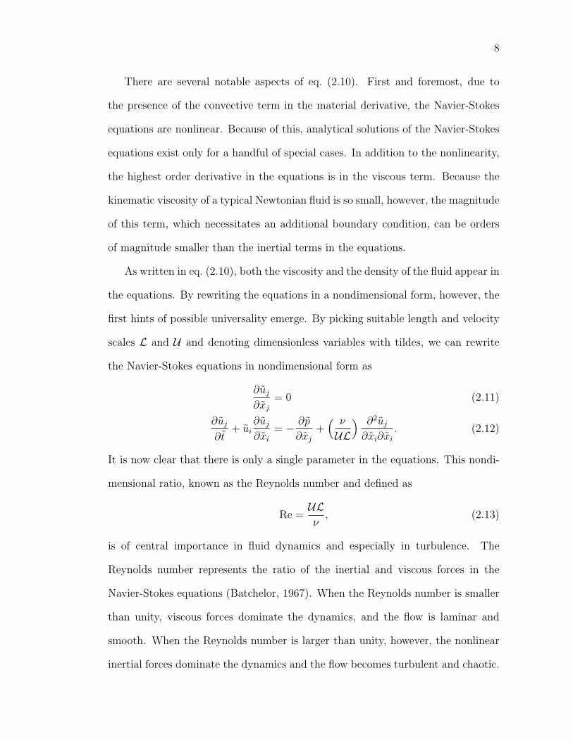
8

There are several notable aspects of eq. (2.10). First and foremost, due to

the presence of the convective term in the material derivative, the Navier-Stokes

equations are nonlinear. Because of this, analytical solutions of the Navier-Stokes

equations exist only for a handful of special cases. In addition to the nonlinearity,

the highest order derivative in the equations is in the viscous term. Because the

kinematic viscosity of a typical Newtonian fluid is so small, however, the magnitude

of this term, which necessitates an additional boundary condition, can be orders

of magnitude smaller than the inertial terms in the equations.

As written in eq. (2.10), both the viscosity and the density of the fluid appear in

the equations. By rewriting the equations in a nondimensional form, however, the

first hints of possible universality emerge. By picking suitable length and velocity

scales L and U and denoting dimensionless variables with tildes, we can rewrite

the Navier-Stokes equations in nondimensional form as

∂uj∂xj

= 0 (2.11)

∂uj

∂t+ ui

∂uj∂xi

= − ∂p

∂xj+( ν

UL

) ∂2uj∂xi∂xi

. (2.12)

It is now clear that there is only a single parameter in the equations. This nondi-

mensional ratio, known as the Reynolds number and defined as

Re =ULν, (2.13)

is of central importance in fluid dynamics and especially in turbulence. The

Reynolds number represents the ratio of the inertial and viscous forces in the

Navier-Stokes equations (Batchelor, 1967). When the Reynolds number is smaller

than unity, viscous forces dominate the dynamics, and the flow is laminar and

smooth. When the Reynolds number is larger than unity, however, the nonlinear

inertial forces dominate the dynamics and the flow becomes turbulent and chaotic.

9

For flows with an externally imposed geometry, relevant velocity and length

scales used to define the Reynolds number are readily apparent. In a pipe flow,

for example, the length scale is usually taken to be the pipe diameter and the

velocity scale to be the mean velocity. Boundaries, however, impose additional

complexity for studying turbulence. For this reason, research in turbulence has

focussed on the case of statistically homogeneous, isotropic flows. In homogeneous

turbulence, flow statistics do not depend on the absolute location in space: only

relative spatial coordinates are relevant. Likewise, in isotropic turbulence statistics

are independent of global rotations. It follows, then, that a homogeneous, isotropic

flow can have no boundaries. There are therefore no externally imposed scales

with which to define the Reynolds number. Instead, intrinsic scales are used. The

velocity scale is taken to be the standard deviation of the velocity field, u′. A

length scale L, known as the integral length scale, is determined by integrating the

velocity autocorrelation function. The resulting Reynolds number ReL = u′L/ν is

therefore based purely on the statistics of the turbulence. For historical reasons,

an additional Reynolds number based on the Taylor microscale λ is often used,

and is given by

Rλ =u′λ

ν=√

15ReL. (2.14)

As mentioned above, high Reynolds number flows are turbulent, and the mo-

tion of individual fluid elements is chaotic. The hallmark of chaos is an extreme

sensitivity to initial conditions, and turbulence is no exception. Even if there were

a general solution to the Navier-Stokes equations, then, any prediction of the sub-

sequent fluid evolution would require the specification of the initial and boundary

conditions to a precision unfeasible for any practical application. Just as in many

other branches of physics and engineering, we are therefore forced into a statistical

10

description of turbulence.

The statistical approach, however, brings its own new difficulties to the prob-

lem. As an example, let us consider the equation of motion for the mean velocity

field, the simplest statistical description of a flow. In order to arrive at this equa-

tion, we simply take the mean of eqs. (2.6) and (2.10), where the symbol 〈·〉 denotes

an ensemble average. The continuity equation is unchanged, since differentiation

commutes with the averaging:

∇ · 〈u〉 = 0. (2.15)

The momentum equations, however, are not as simple. We have

∂〈uj〉∂t

+∂〈uiuj〉∂xi

= −1

ρ

∂〈p〉∂xj

+ ν∂2〈uj〉∂xi∂xi

, (2.16)

where we have used the continuity equation to rewrite the nonlinear term. This

equation contains the quantity 〈uiuj〉, which is not trivially related to the mean

velocity field. Since any quantity can be decomposed into the sum of its mean

value and the fluctuations about the mean, we can write

ui = 〈ui〉+ u′i, (2.17)

where we have used a prime to indicate the fluctuation. In turbulence, this is

known as the Reynolds decomposition (Pope, 2000). The nonlinear term may

then be rewritten as

〈uiuj〉 =⟨[〈ui〉+ u′i][〈uj〉+ u′j]

⟩= 〈ui〉〈uj〉+ 〈u′iu′j〉, (2.18)

since the mean of a fluctuation is zero. Inserting this result into eq. (2.16), we

arrive at

∂〈uj〉∂t

+∂〈ui〉〈uj〉∂xi

= −1

ρ

∂〈p〉∂xj

+ ν∂2〈uj〉∂xi∂xi

−∂〈u′iu′j〉∂xi

. (2.19)

11

These equations are known as the Reynolds Averaged Navier-Stokes (RANS) equa-

tions, and are a basic tool in computational fluid dynamics. The most important

feature of the RANS equations is the appearance of the final term on the right

hand side that involves the correlation of the velocity fluctuations, known as the

Reynolds stress. In the RANS formulation, we have four equations (the continu-

ity equation and the equations of motion of the three components of the mean

velocity), just as in the total Navier-Stokes equations. Unlike the Navier-Stokes

equations, however, which had four unknowns (the pressure and the three compo-

nents of velocity), the RANS equations are underdetermined. The Reynolds stress

adds an extra six unknowns to the system with no corresponding new equations.

This type of difficulty is referred to as a closure problem, and is ubiquitous in the

statistical description of fluid flow. Modeling of the extra unknowns is required to

close the equations of motion, and is therefore of central importance in constructing

a practical, useful description of turbulence.

2.2 Homogeneous, Isotropic Turbulence and Kolmogorov’s

Hypotheses

By far the most important and influential model of turbulence is that of A. N. Kol-

mogorov. Usually referred to simply as K41 theory, Kolmogorov’s 1941 phe-

nomenological model is based on a handful of physically-motivated hypotheses

with surprisingly far-reaching consequences. We note that due to the difficulties

inherent in dealing with boundaries, K41 theory applies only to homogeneous,

isotropic turbulence. In addition, we consider only the fluctuations about the

mean velocity, since these fluctuations are the signature of turbulence.

12

The dynamics of a turbulent flow at scales larger than the integral length scale

L are flow-specific. For smaller scales, however, the flow is thought to become

statistically universal, and the details of how the turbulence was generated are

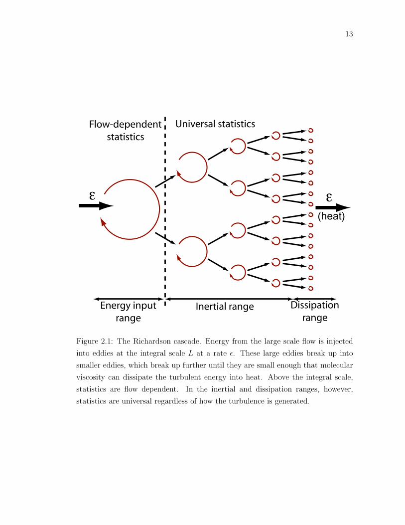
washed away. Classically, the small scale flow is modeled as a cascade process, an

idea first put forward by Richardson (1922). Consider a coherent structure in the

flow of a size comparable to L, which we loosely term an eddy. In the cascade

model, energy is fed to this structure by the non-universal large scales of the flow

at a rate ε, where ε is typically taken to be a power per unit mass. This eddy

is, however, short-lived: due to turbulent fluctuations, it breaks up into smaller

eddies. In the cascade model, this process is presumed to occur with no loss of

energy. These smaller eddies in turn break up into yet smaller eddies, until finally

they are small enough that molecular viscosity can play a role in their dynamics

and dissipate the turbulent energy into heat, again at the same rate ε. At scales

where energy is dissipated, the flow relaminarizes. The Richardson cascade is

illustrated schematically in Fig. 2.1, and is expressed well in Richardson’s (1922)

famous rhyme:

“Big whirls have little whirls,

That feed on their velocity;

Little whirls have lesser whirls,

And so on to viscosity.”

Underlying the cascade model are assumptions of locality of scale and perfect

self-similarity (Frisch, 1995). Each eddy is assumed to have contact only with

those directly larger and smaller than it. Small eddies are merely swept along by

large eddies without being influenced by the large scale motion. In addition, eddies

are assumed to break up into essentially identically smaller copies of themselves.

13

Flow-dependentstatistics

Universal statistics

Energy inputrange

Inertial range Dissipationrange

ε ε(heat)

Figure 2.1: The Richardson cascade. Energy from the large scale flow is injected

into eddies at the integral scale L at a rate ε. These large eddies break up into

smaller eddies, which break up further until they are small enough that molecular

viscosity can dissipate the turbulent energy into heat. Above the integral scale,

statistics are flow dependent. In the inertial and dissipation ranges, however,

statistics are universal regardless of how the turbulence is generated.

14

Kolmogorov (1941a) incorporated these ideas into his similarity hypotheses and

was able to make the cascade model predictive.

Strictly applicable only in the limit of infinite Reynolds number, the Kol-

mogorov (1941a) similarity hypotheses are

1. Hypothesis of Local Isotropy. At scales small compared to the integral

length scale L and far away from any boundaries, turbulence is statistically

homogeneous and isotropic.

2. First Similarity Hypothesis. At scales very small compared to L, turbu-

lence statistics have a universal form determined only by the viscosity ν and

the energy dissipation rate ε. The regime is termed the “dissipation range.”

3. Second Similarity Hypothesis. At scales small compared to L but large

compared to the dissipation scale, turbulence statistics have a universal form

determined only by the dissipation rate ε. This regime is known as the

“inertial range.”

When coupled with dimensional analysis and the theory of isotropic tensors,

the Kolmogorov hypotheses allow the prediction of scaling laws for many of the

quantities of interest in turbulence. K41 theory can also be used to define the

smallest scales of turbulent motion. In the cascade model, the smallest turbulent

scales are those where energy is dissipated by viscous forces. According to the first

similarity hypothesis, such scales can only depend on the viscosity and the dissi-

pation rate. Using dimensional analysis, then, we define the Kolmogorov length

scale η, time scale τη, and velocity scale uη as

η ≡(ν3

ε

)1/4

τη ≡(νε

)1/2

uη ≡η

τη= (εν)1/4. (2.20)

15

We then expect that, statistically, the flow at scales smaller than the Kolmogorov

scales is laminar. This is borne out by the fact that the Reynolds number based

on the Kolmogorov scales, Rη = uηη/ν, is unity.

As discussed above, the cascade model, and therefore K41 theory, is local in

scale. Therefore, the similarity hypotheses can only be applied to statistics that

are similarly local (Batchelor, 1950). It is difficult to determine a priori whether a

given quantity is local in scale. A general rule of thumb, however, is that differences

are local in scale while products are not. As an example, consider the Eulerian

velocity correlation function Rij(r) = 〈ui(x+r)uj(x)〉. This tensor mixes velocities

of all scales, and therefore K41 cannot be applied to it. Indeed, measurements of

Rij(r) show that it decays approximately exponentially with r, while K41 theory

always predicts power laws. Let us consider instead the correlation function of the

velocity differences, Dij(r) = 〈[ui(x+r)−ui(x)][uj(x+r)−uj(x)]〉 = 〈δui(r)δuj(r)〉,

better known as the Eulerian structure function. Since it involves only velocity

differences, this tensor is local in scale. As will be discussed in detail in Chapter

4.2, K41 predicts that, in the inertial range, this tensor should be only a function

of r and the dissipation rate ε. Therefore,

Dij(r) ∼ (εr)2/3, (2.21)

since Dij(r) has units of velocity squared. This power law scaling is well-confirmed

experimentally (Sreenivasan, 1995).

2.3 Beyond K41

Classical K41 theory, as described above, is elegant in its simplicity and its great

utility in generating scaling laws for turbulence statistics. Over the past several

16

decades, however, experiments have made it clear that some of the basic tenets of

the K41 model are violated in real turbulence. A hallmark of turbulent flow is its

“bursty” nature: turbulence is characterized by short-lived but extremely intense

fluctuations of its dynamical quantities. In particular, consider the rate of energy

dissipation rate ε. The classical K41 model assumes in the Second Similarity Hy-

pothesis that 〈ε〉, the mean value of the dissipation rate, is sufficient to characterize

the statistics of inertial range turbulence. As pointed out by Landau (Frisch, 1995),

however, unless ε is constant, 〈εp〉 6= 〈ε〉p and therefore the mean rate of energy

dissipation is insufficient to characterize turbulence. This phenomenon is termed

intermittency. Intermittency is a general feature in nonlinear dynamical systems,

though in turbulence the term has come to refer purely to the large fluctuations

of the dissipation rate.

In response to Landau’s comment, Kolmogorov (1962) introduced the Refined

Similarity Hypothesis, where, based on physical reasoning, he assumed that the

probability density function (PDF) of ε was log-normal. Using this form for the

PDF, he was able to calculate the difference between 〈εp〉 and 〈ε〉p explicitly, finding

that

〈εp〉rεp∼ r−

12µp(p−1), (2.22)

where the average is taken over a volume of linear scale r. In analogy with his

K41 model, Kolmogorov’s intermittency model is known simply as K62. Subse-

quent experiments, however, showed that the predictions of the Refined Similarity

Hypothesis are also not correct (Anselmet et al., 1984), suggesting that ε is not

log-normally distributed. The true PDF of the dissipation rate has proved very

difficult to measure experimentally. Researchers have therefore turned to a reinter-

pretation of the Richardson cascade using fractal ideas (Mandelbrot, 1974; Parisi

17

and Frisch, 1985).

Classical K41 theory assumes that when an eddy in the cascade breaks up,

the smaller eddies it forms occupy the same amount of space as the parent eddy.

Furthermore, it is assumed that the turbulent eddies participating in the cascade

occupy the full volume of turbulent fluid. The dimension of the space occupied by

the eddies is therefore three. But now suppose that when a parent eddy breaks up,

its child eddies do not occupy the same amount of space. In this case, the eddies

will fill only a subspace of the volume of turbulent fluid. Let us suppose that the

space filled by the cascade is characterized by a non-integer fractal dimension D.

This line of reasoning leads to straightforward corrections to K41 scaling laws: if we

consider turbulence statistics at scale r, we must simply weight the corresponding

K41 scaling law by a factor expressing the probability that the point of interest in

the fluid lies in a turbulent eddy of scale r. This probability factor is given by

Pr =( rL

)3−D, (2.23)

where L is the integral length scale, a measure of the size of the maximal volume

of fluid the cascade can occupy (Frisch, 1995). More generally, for turbulence in a

d-dimensional space, we have

Pr =( rL

)d−D, (2.24)

where d−D is known as the codimension. This monofractal model of turbulence

is known as the β-model.

To illustrate the use of the β-model, we again turn to the Eulerian structure

function, following Frisch (1995). Consider the energy at scale r, which we denote

by Er. Using dimensional analysis and the probability factor Pr, we have

Er ∼ u2rPr = u2

r

( rL

)3−D, (2.25)

18

where ur is the velocity at scale r. The flux of energy to smaller scales is given by

Er/tr ∼ u3rPr/r, but is also given by ε ∼ u′3/L, where u′ is the large scale root-

mean-square (RMS) velocity. Therefore, equating these two relations, we have

ur ∼ u′( rL

) 13− 3−D

3 ≡ u′( rL

)h, (2.26)

where h controls the scaling of ur with r/L. We can now write down the the

β-model scaling law for the Eulerian structure function of order p as

〈δu(r)p〉 ∼ uprPr ∼ u′p( rL

)hp+3−D. (2.27)

The β-model does not capture the behavior of real turbulence (Anselmet et al.,

1984), but is the basis for the multifractal model that captures the phenomenology

of turbulence better than any other current model. As a first step, let us consider

a bifractal model. In this case, the turbulent eddies are described not by a single

fractal dimension but by two, and therefore by two different values for h. A given

eddy breaking up will choose to follow the scaling law given by one of the fractal

dimensions with probability µ. The bifractal scaling law for the Eulerian structure

function is then given by

〈δu(r)p〉up

∼ µ1

( rL

)h1p+3−D1

+ µ2

( rL

)h2p+3−D2

. (2.28)

The jump to a multifractal model is straightforward. We now assume that

the cascade chooses its dynamics from a continuous set of fractal dimensions D(h)

indexed by a scaling exponent h that lies in the set I = (hmin, hmax). Extrapolating

from the bifractal case, the scaling law for the Eulerian structure function becomes

an integral over all values of h:

〈δu(r)p〉up

∼∫h∈I

d[µ(h)]( rL

)hp+3−D(h)

. (2.29)

19

As in K41 theory, we suppose that 〈δupr〉 ∼ rζEp . In the inertial range, where this

model should be valid, r � L, and so the smallest exponent in the integral will

dominate. Therefore, we have

ζEp = infh

[hp+ 3−D(h)] . (2.30)

This expression is a Legendre transform between the parameters p and h, and in

principle may be inverted to give

D(h) = infp

[ph+ 3− ζEp

], (2.31)

although this is difficult to apply experimentally due to the, in general, poor de-

termination of the ζEp for a wide range of p (Frisch, 1995). We note that in the

multifractal model, both I and D(h) are a priori unknown, but are presumed to

be universal for all turbulent flows, regardless of the large-scale flow structure.

Chapter 3

Experimental Techniques

3.1 Lagrangian Particle Tracking

Almost everything that is known about turbulence is derived from Eulerian mea-

surements, where probes are fixed with respect to a laboratory reference frame.

Eulerian measurement techniques have become very robust, and standard tech-

niques are well-known. The workhorse of Eulerian measurement devices is the hot

wire anemometer, introduced as early as 1909 (King, 1914). In its most basic form,

the hot wire anemometer consists of a small metal wire heated by the application

of a voltage. As the fluid sweeps past the wire it advects away heat, requiring the

adjustment of the applied voltage in order to regulate the wire temperature. King

(1914) worked out the relation between the applied voltage and the fluid velocity.

Hot wire anemometry is well suited to measurements in gas flows, and is the stan-

dard tool for wind tunnel measurements. Hot wires do not work well, however, in

liquid flows.

A whole host of new Eulerian measurement techniques is opened up by the

addition of neutrally buoyant passive tracer particles to the flow. This is, in general,

easier to accomplish in liquid flows rather than gas flows, but some techniques do

exist for creating passive tracers for gas flows as well (Poulain et al., 2004). One

elegant technique for making Eulerian measurements in a flow seeded with tracers is

Laser Doppler Anemometry (LDA), also referred to as Laser Doppler Velocimetry

(LDV). LDA uses the coherence of laser light to make direct measurements of the

fluid velocity. By focussing two laser beams on a small spot in the flow, they

will interfere and produce a fringe pattern. When a tracer particle (and ideally

20

21

only one at a time) passes through the measurement volume, it produces a burst

of flickering reflected light. The frequency of the flickering of this reflected light

depends only on the wavelength of the laser light and the crossing angle of the

beams, both known quantities, as well as the velocity of the particle normal to the

fringes. Measuring the flicker frequency therefore directly gives a single component

of the particle velocity. By using multiple pairs of beams, all three components of

the Eulerian velocity can be measured simultaneously.

Seeding a flow with passive tracers is also the basis for the Eulerian technique

Particle Image Velocimetry (PIV). PIV has become a very popular tool in indus-

try and in the engineering community, and is well suited to characterizing complex

mean flow patterns or microfluidic flows, where the effects of turbulence are min-

imal. The tracer particles are illuminated by a laser sheet and a camera is used

to take two images of the flow spaced very closely in time. By assuming that

nearby particles move similarly, average velocity vectors for groups of particles are

estimated, usually from the cross-correlation of the two images (Adrian, 1991).

PIV usually measures only two components of the velocity, though stereoscopic

and holographic PIV systems have been developed to measure all three velocity

components (Hinsch and Hinrichs, 1996).

Eulerian measurements have been very important in the development of the

theory of turbulence, but a complete understanding of turbulence is not possible

without corresponding Lagrangian information. Lagrangian measurements require

identifying individual fluid elements and measuring flow statistics along their tra-

jectories. Although some progress has been made in tagging and following true

fluid elements (Pashtrapanshka and van de Water, 2005), passive tracer particles

similar to those used in LDA and PIV are commonly employed as approximations

22

of true fluid elements. The motion of these tracers may then be followed to ex-

tract Lagrangian trajectories, a technique known as Lagrangian Particle Tracking

(LPT). It is common to use several detectors in LPT system, in order to resolve

all three components of the motion of the particles.

LPT systems have been designed using many different types of detectors. In the

present work, we image the tracer particles optically. Acoustic LPT methods have

also been used (Mordant et al., 2001), though they measure the particle velocity

directly and must integrate the velocity tracks to find the particle positions. For

geophysical flows, Lagrangian tracers may be tracked by radio beacons, radar

(Hanna, 1981), or the Global Positioning System.

In general, there are three algorithmic components of an optical LPT system.

First, individual particles must be identified in the image space of each detector.

Next, the two-dimensional information from each detector must be combined to

generate 3D information for each particle coordinate. Finally, the motion of the

particles must be tracked in time. The last two steps may be logically interchanged;

there are, however, good reasons for presenting them in this order, as will be

discussed below.

Optical LPT systems have been used for many years. The first such systems

consisted of photographs of tracer particles that were analyzed by hand (Chiu

and Rib, 1956). Modern optical LPT systems use digital cameras and process the

images using computer algorithms to accomplish the LPT tasks outlined above.

Most such digital cameras, however, are not fast enough to resolve the fastest

time scales of the turbulent motion at high Reynolds numbers. Previously, the

Bodenschatz research group has adapted the silicon strip detectors used in the

vertex detectors in high energy particle accelerators to the LPT problem, with

23

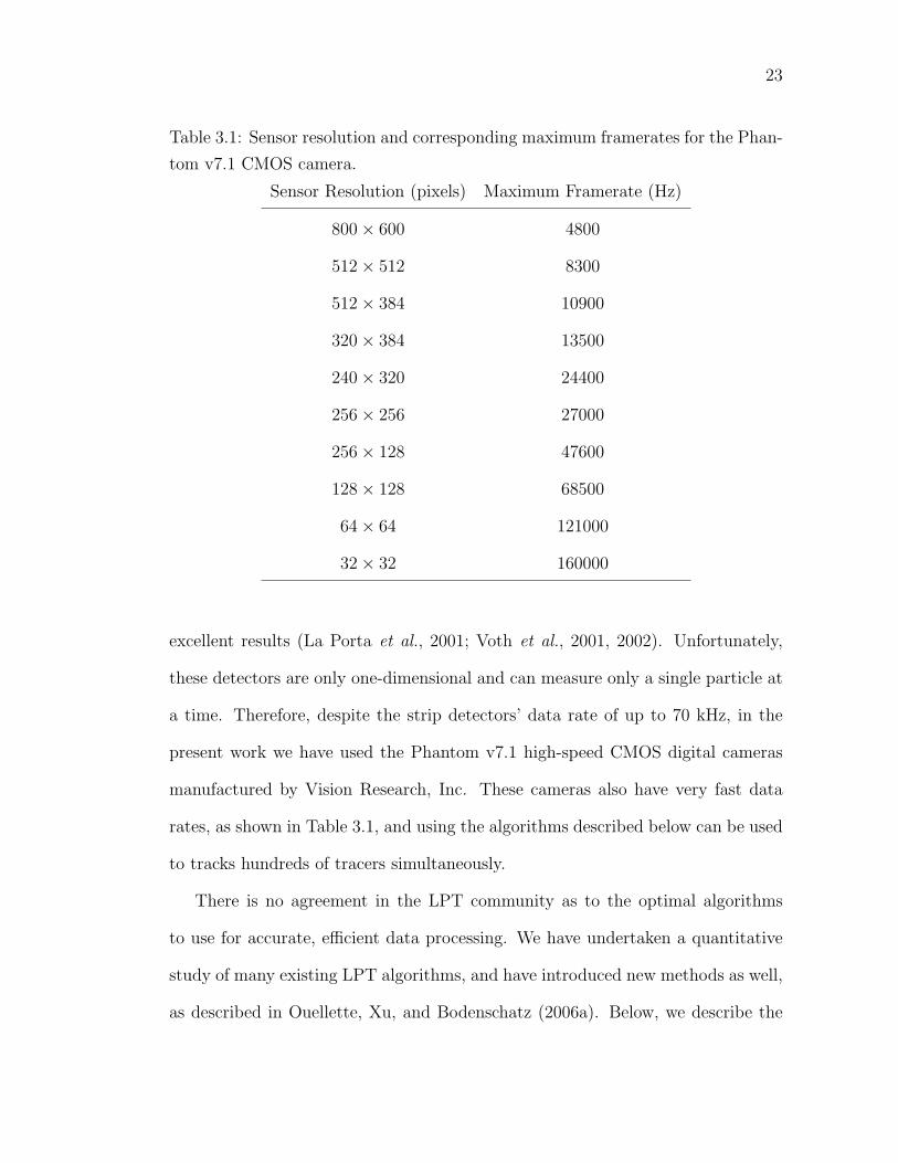
Table 3.1: Sensor resolution and corresponding maximum framerates for the Phan-

tom v7.1 CMOS camera.

Sensor Resolution (pixels) Maximum Framerate (Hz)

800× 600 4800

512× 512 8300

512× 384 10900

320× 384 13500

240× 320 24400

256× 256 27000

256× 128 47600

128× 128 68500

64× 64 121000

32× 32 160000

excellent results (La Porta et al., 2001; Voth et al., 2001, 2002). Unfortunately,

these detectors are only one-dimensional and can measure only a single particle at

a time. Therefore, despite the strip detectors’ data rate of up to 70 kHz, in the

present work we have used the Phantom v7.1 high-speed CMOS digital cameras

manufactured by Vision Research, Inc. These cameras also have very fast data

rates, as shown in Table 3.1, and using the algorithms described below can be used

to tracks hundreds of tracers simultaneously.

There is no agreement in the LPT community as to the optimal algorithms

to use for accurate, efficient data processing. We have undertaken a quantitative

study of many existing LPT algorithms, and have introduced new methods as well,

as described in Ouellette, Xu, and Bodenschatz (2006a). Below, we describe the

24

tests of the various algorithms in detail. We begin with algorithms to determine

the positions of the tracers on the detector, continue with a description of the

algorithm we use for stereomatching of the images from multiple cameras, and

finally present algorithms for particle tracking itself.

3.1.1 Particle Finding Problem

The accuracy of an LPT system depends crucially on the precision with which the

tracer particles can be identified in the camera images. In general, it is sufficient

to determine the coordinates of the particle centers. An ideal particle finding

algorithm must meet several criteria:

1. Sub-pixel accuracy. When the particle images cover several pixels, the center

of the particle may be found to within a fraction of a pixel.

2. Speed. Due to the extremely high data rate from the detectors necessary for

the measurement of an intensely turbulent flow, a particle finding algorithm

must be efficient and fast.

3. Overlap handling. When the images of multiple particles overlap on a single

detector plane, it becomes more difficult to determine the particle centers. A

good particle finding algorithm must remain effective for locating the centers

of clusters of overlapping particle images.

4. Robustness to noise. Even the best cameras have some background noise

in the images. A particle finding algorithm must locate the particle centers

accurately even for moderate noise levels.

It is common to assume that every local maximum in image intensity above

some threshold corresponds to a particle, and we make this assumption in this

25

analysis. The simplest method, then, for determining a particle center is simply

to pick the center of this local maximum pixel. This method is certainly fast, can

handle overlap, and is moderately robust to noise. The accuracy of this method,

however, is very poor: no sub-pixel resolution is possible. Many classes of more

intelligent algorithms have been proposed, including weighted averaging schemes

(Maas et al., 1993; Maas, 1996; Doh et al., 2000), function fitting (Cowen and

Monismith, 1997; Mann et al., 1999), and template matching (Guezennec et al.,

1994), as well as the standard PIV technique of image cross-correlation (Adrian,

1991; Westerweel, 1993). Template matching suffers if all particle images are not

the same size, and is suitable only for experiments using laser sheets to illumi-

nate their tracers. Since we illuminate three-dimensional volumes of the flow, we

shall not consider template matching algorithms. Cross-correlation techniques are

more suited to very densely seeded flows, and so we shall also not consider them.

Below, we shall compare a weighted averaging algorithm with both one- and two-

dimensional Gaussian fitting and a neural network-based technique. We shall first

discuss the algorithms being tested in more detail.

Description of Algorithms

Weighted averaging is a very simple technique, and is therefore widely employed

in LPT systems. Camera images must first be segmented into contiguous groups

of bright pixels, representing ideally single particles. The coordinates (xc, yc) of

the center of the pixel group are then determined by averaging the positions of all

the pixels in the group weighted by their intensity grey values. More precisely, if

we let I(x, y) be the intensity of the pixel at (x, y), xc is given by

xc =

∑p xpI(xp, yp)∑p I(xp, yp)

, (3.1)

26

similar to the determination of the center of mass of a cluster of point masses. yc

is defined similarly.

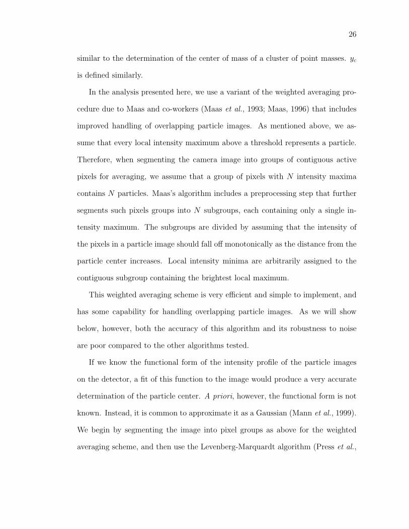
In the analysis presented here, we use a variant of the weighted averaging pro-

cedure due to Maas and co-workers (Maas et al., 1993; Maas, 1996) that includes

improved handling of overlapping particle images. As mentioned above, we as-

sume that every local intensity maximum above a threshold represents a particle.

Therefore, when segmenting the camera image into groups of contiguous active

pixels for averaging, we assume that a group of pixels with N intensity maxima

contains N particles. Maas’s algorithm includes a preprocessing step that further

segments such pixels groups into N subgroups, each containing only a single in-

tensity maximum. The subgroups are divided by assuming that the intensity of

the pixels in a particle image should fall off monotonically as the distance from the

particle center increases. Local intensity minima are arbitrarily assigned to the

contiguous subgroup containing the brightest local maximum.

This weighted averaging scheme is very efficient and simple to implement, and

has some capability for handling overlapping particle images. As we will show

below, however, both the accuracy of this algorithm and its robustness to noise

are poor compared to the other algorithms tested.

If we know the functional form of the intensity profile of the particle images

on the detector, a fit of this function to the image would produce a very accurate

determination of the particle center. A priori, however, the functional form is not

known. Instead, it is common to approximate it as a Gaussian (Mann et al., 1999).

We begin by segmenting the image into pixel groups as above for the weighted

averaging scheme, and then use the Levenberg-Marquardt algorithm (Press et al.,

27

1992) to fit the function

I(x, y) =I0

2πσxσyexp

{−1

2

[(x− xcσx

)2

+

(y − ycσy

)2]}

, (3.2)

where σx and σy are the Gaussian widths in the horizontal and vertical directions.

If a pixel group contains N local maxima, we simply fit the sum of N Gaussians

to the group.

This method is very accurate and handles overlap well. It is, however, sig-

nificantly more computationally intensive than the other methods studied, taking

approximately a factor of four more time in our tests. Additionally, this 2D Gaus-

sian fit requires large particle images. Inspection of eq. (3.2) shows that each

Gaussian requires the determination of five parameters, namely the overall inten-

sity I0, the widths σx and σy, and the centers xc and yc. At minimum, then, the

pixel group must contain at least 5N pixels for a fit to be possible, and more for the

fit to be accurate. Small particle images must then either be ignored or processed

with a different method.

A more efficient and less demanding approximation of a full 2D Gaussian fit

can be accomplished by using instead two 1D Gaussians (Cowen and Monismith,

1997). We fit single 1D Gaussians to the horizontal pixel coordinates and the

vertical coordinates in turn. Each Gaussian has only three fit parameters, as

opposed to the five needed by the 2D Gaussian, and so smaller particle image sizes

are sufficient. In addition, unlike in the 2D case, we can find an analytical solution

for the particle center based on only the local maximum pixel and its closest

horizontal and vertical neighbors. Labeling the horizontal pixel coordinates x1, x2,

and x3, where x2 is the coordinate of the local maximum, we can solve the system

28

of equations

Ii =I0√2πσ

exp

[−1

2

(xi − xcσx

)2]

(3.3)

for i = 1, 2, 3 to give

xc =1

2

(x21 − x2

2) ln(I2/I3)− (x22 − x2

3) ln(I1/I2)

(x1 − x2) ln(I2/I3)− (x2 − x3) ln(I1/I2). (3.4)

The vertical coordinate of the particle center is defined analogously. This 1D Gaus-

sian Estimator retains much of the accuracy of the 2D Gaussian fit but at only a

fraction of the computational cost. The image segmentation step required for the

2D fit can be omitted, and only the particle center needs to be computed, with

the fit parameters I0, σx, and σy left undetermined. Additionally, inspection of

eq. (3.4) shows that the coordinates of the particle centers depend only on the co-

ordinates of the three pixels used in the fit and the natural logarithms of the pixel

intensities. Since the cameras are digital, however, the pixel intensities are quan-

tized, and therefore all necessary logarithms may be precomputed once and used

for the determination of all the particle centers. Use of the 1D Gaussian Estimator

therefore requires only a few multiplications, and is therefore very efficient.

In addition to the algorithms described above, we have also developed a neural

network-based approach to the particle finding problem. Neural networks are a

class of machine learning algorithms based on a crude model of the human brain,

and hope to exploit some of the same properties that make the brain such a pow-

erful computer. The brain can be viewed as a massively parallel computational

network consisting of roughly 1011 interconnected neurons that is capable of, among

other things, learning and generalization. A neural network is constructed simi-

larly, consisting of many interconnected nodes arranged in layers. In the machine

learning and artificial intelligence community, neural networks are known to be

29

very effective in pattern matching and classification applications. In general, a

neural network can be applied to a problem when the function to be evaluated (or

“learned” by the network) has a fixed number of inputs and outputs that can be

normalized to fall in a known range, when valid input/output pairs may be gen-

erated for training, when a slow one-time learning period is acceptable, and when

fast evaluation of the function may be necessary. Within these general criteria,

neural networks are very flexible. The function to be learned may be discrete-,

real-, or vector-valued, or some combination. The input/output pairs used for

training the network may contain errors, and the resulting networks are usually

very robust to noise in the input data. It is important to note, however, that due

to the complexity of a fully trained neural network, the programmer will in general

not understand what function the network is evaluating. When such understand-

ing is not required, and when the criteria above are fulfilled, neural networks can

be very powerful tools.

Formally, a neural network is a directed, acyclic graph. The nodes of the

graph, termed “neurons” in analogy with the brain, may have input connections

only (output neurons), output connections only (input nodes), or both (hidden

neurons). Every edge in the graph has an associated weight w represented by a

real number with −1 ≤ w ≤ 1. “Training” the network refers to adjusting the

weights in order to produce the desired output.

A neural network is specified by three pieces of information: the graph topology,

the neuron activation function, and the training algorithm used. Neurons are

arranged in layers. Every network will contain both an input layer and an output

layer, and may contain one or more hidden layers. Input information is fed into

the input layer, and the evaluated function values are read from the output layer.

30

Hidden layers allow the network to perform complex tasks.

The neuron activation function maps the input value of a given neuron to its

output value. The simplest activation function is a step function. Let us consider

a neuron with N input connections labeled x1 to xN . Each input connection also

carries an edge weight wi, where i ranges from 1 to N . Then the step function

activation is given by

o(x1, . . . , xN) =

1,∑N

i=1wixi ≥ 0

−1,∑n

i=1wixi < 0. (3.5)

Training such a neuron is simple. For each training cycle, the weights of all the

input edges are updated as

wi ← wi + ∆wi, (3.6)

where ∆wi is given by

∆wi = η(t− o)xi. (3.7)

Here t denotes the target output and o the neuron output. η is a constant known

as the learning rate that controls how much the network can change over one

training iteration. Such a simple neuron is known as a perceptron, and can exactly

represent, for example, any Boolean function (Mitchell, 1997).

For more complex functions, however, more complex networks are required. In

particular, networks where the activation function is linear in the input values,

such as that described above for perceptrons, can only represent linear function.

For nonlinear problems, we must use nonlinear activation functions. A common

choice is a sigmoid function,

o(x1, . . . , xN) =1

1 + exp(−∑N

i=1 wixi

) . (3.8)

31

In addition, we can introduce one more hidden layers, that further enhance the

nonlinear capabilities of the network. In general, continuous functions may be ap-

proximated arbitrarily well by networks with a single hidden layer, while arbitrary

function may be represented with only two hidden layers (Mitchell, 1997), a result

that follows from work of Kolmogorov (1957).

With complex networks, we must specify more complex training procedures.

The standard training algorithm for such multilayer networks is the backpropaga-

tion algorithm. Let us define the total network error as the sum of the errors of

each individual output neuron for all the training examples, given by

E(w1, . . . , wN) =1

2

∑d∈D

∑k∈outputs

(tkd − okd)2, (3.9)

where N is the number of output neurons, D is the set of all training examples,

and k runs over the set of output neurons. The backpropagation algorithm then

proceeds as follows, for each training example (xi, ti). First, the input values xi

are fed into the network, and an output value ou is computed for each neuron u.

Next, an error δk is calculated for each output neuron k, given by

δk = ok(1− ok)(tk − ok). (3.10)

This error is then propagated back through the network and an error is calculated

for each hidden neuron h, given by

δh = oh(1− oh)∑k

wkhδk. (3.11)

Finally, the edge weights are updated as

wji ← wji + ∆wji, (3.12)

where ∆wji is given by

∆wji = ηδjxji, (3.13)

32

which amounts to a gradient descent method for finding a local minimum in the

error surface, a method justified by Bayes’ Theorem. Since gradient descents are

susceptible to becoming stuck on flat surfaces or local minimum, a “momentum”

term is often added to the standard backpropagation algorithm. Equation (3.13)

then becomes

∆wji(n) = ηδjxji + α∆wji(n− 1), (3.14)

where α is the momentum and n indexes the training iteration. For more infor-

mation on neural networks, the reader is referred to Mitchell’s (1997) book.

Neural networks have been applied to both the particle tracking problem (Grant

and Pan, 1997; Chen and Chwang, 2003; Labonte, 1999, 2001) and the stereo-

matching problem (Grant et al., 1998) before. Carosone et al. (1995) applied the

Kohonen neural network to the problem of distinguishing images of isolated parti-

cles from those of overlapping particles. In the present work, we solve the particle

finding problem completely using a neural network.

The network used sigmoid neurons arranged in an input layer of 81 neurons,

a single hidden layer of 60 neurons, and an output layer of two neurons. The

input to the network was a 9 × 9 pixel subwindow of the camera image centered

on a local intensity maximum. The two output neurons report the horizontal and

vertical coordinates of the particle center. By asking the network to find only

single particles at a time, the problem of fixing the number of inputs and outputs

was solved. If the network had been fed the entire camera image, the number

of outputs would not be known. In addition, the network was trained to find

particles near the center of the window, so that overlap could be handled simply

by centering the window on each local maximum in turn. The 9× 9 pixel window

was chosen so that full particle images would definitely be contained in the window;

33

small changes to the size of this window should not affect the performance of the

network. The network was trained using the backpropagation algorithm described

above augmented with a momentum term.

Training the network is a slow operation, but subsequent computation of the

particle centers is fast. The network handles cases of overlap well. As will be

shown below, the network is also very robust to noise, as is generally the case with

neural networks.

Tests of the Algorithms

A quantitative test of the four particle finding algorithms presented above is not

possible without images where the true positions of the particle centers are known.

This requirement precludes the use of real experimental images for testing pur-

poses. Instead, we have generated synthetic images computationally. This ap-

proach also allows us to study the effects of changing different aspects of the

images rigorously and independently.

Images were generated assuming one of two intensity profiles for the particle

images. The assumed intensity profile was discretized by integrating over each

pixel, just as the true intensity profile would be.

The two intensity profiles used in these tests were a Gaussian and an Airy

pattern. Gaussian profiles are often used in tests of particle finding algorithms,

introducing a bias towards Gaussian fitting routines. The true intensity profile is,

however, most likely well approximated by a Gaussian (Westerweel, 1993; Cowen

and Monismith, 1997). To mitigate the effects of any bias we have also used Airy

patterns. Generated by diffraction from a circular aperture, the Airy pattern is

given by (J1(r)/r)2, where J1(r) is the cylindrical Bessel function of order 1 and r

34

Figure 3.1: Sample portions of images generated with different intensity profiles.

Image (a) used Gaussian intensity profiles, while image (b) used Airy pattern

profiles.

is the distance from the particle center. The ratio of the Gaussian width and the

radius of the first peak of the Airy pattern was fixed at 0.524 to equalize the energy

in the 2D Gaussian and the first peak of the 2D Airy pattern. By equalizing the

energy rather than the width of the two intensity profiles, we ensure that they are

very different, and thus better for testing the performance of the various algorithms

under very different conditions.

Images were generated on a 256 × 256 pixel grid, the same size images as

were used in our actual experiment. Each pixel intensity was stored as an 8 bit

greyscale value, for a total of 256 possible intensity grey values. In every case,

the particle intensity maxima were sampled from a Gaussian distribution centered

at 180. Portions of an image generated with Gaussian intensity profiles and Airy

patterns are shown in Fig. 3.1. For some sets of images, additive white Gaussian

noise was introduced into the images. The central limit theorem suggests that

Gaussian noise should be a good approximation for the noise in real images, after

35

all the many possible sources of image noise are compounded.

The neural network described above was trained only on images with Gaussian

intensity profiles, in an attempt to make their baseline performance comparable

to the Gaussian fitting routines. Other characteristics of the training images,

including particle seeding density, particle image size, and noise levels, were varied.

In order to quantify the performance of the four algorithms, errors were cal-

culated by finding the difference between the true particle centers and the cal-

culated centers for the horizontal and vertical components independently. The

distributions of these errors were symmetric with mean zero in all cases, and the

distributions for the horizontal and vertical components were identical, showing

no bias. For the purpose of comparing the algorithms as a function of the image

parameters, we define a parameter ∆ given by∫ ∆/2

−∆/2

P (x)dx = 0.8, (3.15)

where P (x) is the PDF of the error as a function of the distance x from the true

particle center. ∆ measures the radius of the circle around the true particle center

containing 80% of the measured errors. In addition to measuring the errors of the

algorithms, we have also measured the yield of the algorithms, defined as the ratio

of identified particles to the total number of particles in the image.

Four aspects of the particle images were tested independently. The results of

varying the particle seeding density from 150 particles per image to 600 particles

per image are shown in Fig. 3.2. For this test, the particle image half-width was

fixed at 0.8 pixels. No noise was added to these images.

Increasing the seeding density increases the likelihood of particle overlap, mak-

ing the particle finding problem more difficult. Since overlapping particle images

are significantly more difficult to handle than isolated particles, the accuracy should

36

decrease as the seeding density increases. As seen in Fig. 3.2, this is indeed the

case, although the error increase is only moderate. The two Gaussian fitting al-

gorithms performed almost equally well while the weighted averaging algorithm

performed by far the poorest. The neural network method fell in between the

other three in terms of accuracy. In addition, we note that the accuracy of the two

Gaussian fitting methods and the neural network method decreased when Airy pat-

tern intensity profiles were used. The accuracy of the weighted averaging method,

however, was actually improved when applied to the Airy pattern images. This

may because the strong central peak of the Airy pattern weighted the central pixel

more heavily than the Gaussian intensity profile.

Focusing on the error only suggests that a seeding density of 600 particles per

256×256 pixel image is acceptable for LPT. The yield, however, drops very quickly

as the seeding density increases, as shown in Fig. 3.2, dropping as low as 68% for

the weighed averaging method. For this reason, for the rest of the simulated images

used we considered a seeding density of only 300 particles per image, given that

all four algorithms maintained a yield of over 90% at this seeding density.

As with increasing the seeding density, larger particle images lead to more

overlap and therefore a more difficult problem. On the other hand, larger particle

images provide more information to the center finding algorithm, and can therefore

lead to increased accuracy. A balance must be struck between these two effects.

In Fig. 3.3 we show the performance of the four algorithms as a function of

particle image size. As mentioned above, the number of particles per image was

fixed at 300, and no noise was added to any of these images.

For the data sets using Gaussian intensity profiles, the error showed a minimum

at a half-width between 0.7 and 0.9 pixels for both of the Gaussian fitting methods

37

Figure 3.2: The effects of particle seeding density. The error of the four algorithms

increases with the number of particles in each 256 × 256 pixel image for both

Gaussian intensity profiles (a, c) and Airy pattern profiles (b,d). The yield of the

algorithms shows a stronger dependence on particle seeding density. Symbols: �

Weighted Averaging; • 2D Gaussian Fit; N 1D Gaussian Estimator; H Neural

Network.

38

and for the neural network. The behavior of the weighted averaging algorithm is

more varied. The peak in error at a particle image half-width of 0.7 pixels may

perhaps be explained by the introduction of significant levels of overlap while at

the same time maintaining very small clusters of pixels in each particle image.

Different behavior is seen for the images generated with Airy pattern intensity

profiles. For the two Gaussian fitting methods, the error peaked at about 0.8

pixels, and decreased for larger particle images. This may perhaps be explained by

considering that larger Airy patterns appear more Gaussian around their peaks.

The neural network and weighted averaging methods have a similar peak in error,

though at larger particle sizes. In addition, both algorithms performed significantly

worse on very small particle images. We also note that the weighted averaging

method gave better results when applied to the particle images generated with

Airy patterns, as found above as a function of particle seeding density.

After testing the performance of the four algorithms on noiseless images, we

fixed the particle image half-width at 0.8 pixels and the seeding density at 300

particles per image and added noise to the simulated camera images. In a real

LPT system, noise will be introduced into the images in the form of errors from

the camera sensor, thermal noise in the electronics, shot noise in the detection

of the photons scattered from the tracer particles, and many other sources. The

central limit theorem states that as all the various noise sources are compounded,

the distribution of the noise will approach a Gaussian. For that reason, we have

chosen to apply additive white Gaussian noise to our simulated images.

By fixing the mean of the added noise at zero and varying the standard devia-

tion of the noise, we have tested the sensitivity of the four algorithms to fluctua-

tions in the noise level, shown in Fig. 3.4. As expected, as the standard deviation

39

Figure 3.3: The effects of particle image size on the four algorithms. Plots (a)

and (c) were generated with Gaussian intensity profiles, while plots (b) and (d)

were generated with Airy pattern profiles. Symbols: �Weighted Averaging; • 2D

Gaussian Fit; N 1D Gaussian Estimator; H Neural Network.

40

Figure 3.4: The effects of changing the standard deviation of additive white Gaus-

sian noise. For Gaussian intensity profiles, the Neural Network performs nearly

as well as the 2G Gaussian Fit algorithm for both Gaussian intensity profiles (a,

c) and Airy pattern profiles (b, d) while maintaining high yields as the standard

deviation of the noise increases. Symbols: � Weighted Averaging; • 2D Gaussian

Fit; N 1D Gaussian Estimator; H Neural Network.

of the noise was increased, both the accuracy and the yield of all the algorithms

decreased. The yield of the 2D Gaussian fit algorithm dropped very quickly with

noise level when Airy pattern intensity profiles were used. We note, however, that

the performance of the neural network degraded slower than that of the other

algorithms, beating the 1D Gaussian estimator for high noise levels and Gaus-

sian intensity profiles and nearly matching both Gaussian methods for Airy patter

intensity profiles.

41

In addition to varying the standard deviation of the noise, we have also fixed

the noise fluctuations and varied the mean noise level, corresponding to changing

the level of background noise. We have fixed the noise standard deviation at 5.6,

corresponding to 2.5 bits of noise, a typical value in our cameras. The performance

of the four algorithms as a function of mean noise is shown in Fig. 3.5.

The weighted averaging method and both Gaussian fitting methods showed

sensitivity to the mean noise level, though less than they had to the noise standard

deviation. The neural network, however, showed almost no changes as the mean

noise was increased when Gaussian intensity profiles were used, and only a slow

degradation when Airy pattern intensity profiles were used. Coupled with its

slow degradation as a function of noise standard deviation, the neural network is

significantly more robust to noise than the other algorithms tested.

We may draw several conclusions from the analysis presented above. In all

cases, the weighted averaging algorithm is significantly less accurate than the other

three algorithms tested. Given that it is also no faster or easier to implement

than the 1D Gaussian Estimator, it should not be used in LPT systems. The 1D

Gaussian Estimator is also preferable to the 2D Gaussian fit. The two algorithms

have comparable accuracy, but the 1D Gaussian Estimator runs at least a factor

of four faster and has a higher yield of correctly found particles in all cases.

While the 1D Gaussian Estimator also outperformed the neural network in

the absence of noise, the network was far more robust to both changes in mean

background noise and to noise fluctuations. We also note that the performance of

the neural network was roughly the same when applied to images generated with

Gaussian intensity profiles, which the network had been trained on, and images

generated with Airy pattern intensity profiles. It is therefore reasonable to assume

42

Figure 3.5: The effects of changing the mean noise level. While the Weighted Aver-

aging and both Gaussian algorithms lose accuracy as the mean background noise

increases, the Neural Network is almost unaffected for both Gaussian intensity

profiles (a, c) and Airy pattern profiles (b, d). Symbols: � Weighted Averaging;

• 2D Gaussian Fit; N 1D Gaussian Estimator; H Neural Network.

43

that the network can properly generalize to finding particles in real images when

trained on synthetic images.

Since the noise levels in our cameras are very low, we have chosen to use the

1D Gaussian Estimator to locate the particle centers in the camera images, and

we conservatively estimate that the algorithm can find the true particle centers to

within 0.1 pixels. In LPT systems with higher noise levels, however, the neural

network scheme would be preferable.

3.1.2 Stereoscopic Reconstruction

After determining the 2D coordinates of the particles on each of the camera image

planes, a stereomatching process must be used to reconstruct the 3D coordinates of

the particles in the laboratory reference frame. In an LPT experiment, the tracer

particles have no distinguishing features that can be used to aid in this recon-

struction. Instead, the only information that can be used is the photogrammetric

condition that, for each camera, the camera projective center, the particle coor-

dinates on the image plane, and the particle coordinates in the laboratory frame

must be collinear (Maas et al., 1993). Furthermore, these lines of sight from all

the cameras will intersect at the true location of the particle.

Ambiguities can arise in this stereomatching process if multiple particles lie

on the same line of sight. This case will arise more frequently when the density

of particles in the measurement volume is high. Employing more cameras will

help alleviate this problem. Dracos (1996) has shown that for a reasonable par-

ticle seeding density, at least three cameras are needed in order to resolve these

ambiguities.

The stereomatching algorithm we use is based on those of Dracos (1996) and

44

Mann et al. (1999). Consider a particle image pi on one detector. As described

above, we can project a line of sight from the perspective center of the camera

through the particle image. We then in turn project this line of sight onto the

image planes of the other cameras. Particle images on these images planes that

fall within some tolerance ε are considered possible matches to pi. In this fashion,

a list of possible matches for pi is constructed for every other camera in the system.

This process is then repeated for every particle image on every detector. The lists

are then checked for consistency, and the 3D coordinates are found.

3.1.3 Particle Tracking

After both finding the 2D positions of the tracer particles and stereomatching them

to find the full 3D positions, the particles must be tracked in time. In its most

general form, the problem of tracking many particles over many frames is a mul-

tidimensional assignment problem. Such multidimensional assignment problems

are known to be NP-hard for more than two dimensions (Veenman et al., 2003).

There is therefore no known tractable algorithm for solving the full problem. Par-

ticle tracking algorithms are instead forced to approximate the optimal solution

of the full assignment problem by restricting the temporal scope of the tracking,

considering only a few frames at a time.

Let xni denote the ith particle position in the nth frame. A tracking algorithm

attempts to find an xn+1j for each xni such that xj is the position of the particle in

frame n + 1 that was at the position xi in frame n. In order to make this match

correctly, we define a cost φnij for each pair of xn+1j and xni . This cost is one of the

quantities that differentiates tracking algorithms. In general, the optimal solution

to the tracking problem will be given by creating links between the xn+1j and xni

45

so that the total cost

Φ =∑n

∑i

∑j

φnij (3.16)

is minimized. As discussed above, however, the full solution is intractable, and so

we restrict range of n, minimizing the cost for only a few frames at a time. This

type of approximation is generally known as a greedy matching approximation

(Veenman et al., 2001). A different class of algorithms employs iterative schemes,

attempting to minimize the total cost Φ by making an initial guess at the proper

links and then swapping pairs of links in an attempt to find a better solution (Sethi

and Jain, 1987; Ohmi and Li, 2000). These iterative schemes work well for some

simpler machine vision problems, but are unsuitable for LPT due to the desired

long particle tracks.

In addition to restricting the number of frames considered at a time, most

tracking algorithms also restrict the xn+1j considered for each xni by imposing a

limit on the distance a particle can travel from one frame to the next.

Within these approximations, a tracking algorithm is specified by the number

of frames considered at a time, the heuristic used to calculate the cost φnij and

the method used to break tracking conflicts. A conflict occurs whenever the same

particle in frame n + 1 is the best match for multiple particles in frame n. These

conflicts do not, in general, stem from overlapping particle images, since we track

in 3D: overlapping images will have been resolved by the stereomatching algorithm.

In the present work, we consider four different tracking heuristics and two types

of conflict breaking. In general, particle tracking heuristics depend on particu-

lar properties of the tracer particles, such as velocity and acceleration, changing

smoothly and slowly. We describe the individual tracking heuristics tested below,

and illustrate them in Fig. 3.6. We note that many of these tracking heuristics

46

rely on sections of partially completed track; in all cases, the first two frames were

matched together using the Nearest Neighbor algorithm.

1. Nearest Neighbor (NN). The tracking cost is given by the distance between

the point in frame n and the point in frame n+ 1, namely

φnij =∥∥xn+1

j − xni∥∥ . (3.17)

2. 3 Frame: Minimum Acceleration (3MA). The position of the particle in frame

n− 1 is used along with the position in frame n to estimate a local velocity

for the particle, which is then used to extrapolate an estimated position xn+1i

for the particle in frame n+ 1, given by

xn+1i = xni + vni ∆t, (3.18)

where vni is the estimated velocity and ∆t is the time elapsed between frames.

The tracking cost,

φnij =

∥∥xn+1j − 2xni + xn−1

i

∥∥2∆t2

, (3.19)

is calculated for all the possible matches falling in some search volume sur-

rounding the estimate, and is given by the estimated particle acceleration

(Malik et al., 1993; Dracos, 1996).

3. 4 Frame: Minimum Change in Acceleration (4MA) The expected position of

the particle in frame n + 1 is estimated in the same fashion as in the 3MA

algorithm. For each particle in the search volume in frame n+ 1, a position

xn+2i in frame n+ 2 is estimated kinematically as

xn+2i = xni + vni (2∆t) + ani (2∆t)2. (3.20)

47

A new search volume around this position is created, and particles in this

volume are investigated. The tracking cost is given by the change in accel-

eration from frame n + 1 to frame n + 2 (Malik et al., 1993; Dracos, 1996),

namely

φnij =1

2∆t2{∥∥xn+2

j − 2xn+1j + xni

∥∥− ∥∥xn+1j − 2xni + xn−1

i

∥∥} . (3.21)

4. 4 Frame: Best Estimate (4BE) This new algorithm is similar to the 4MA

algorithm in structure, but with a different cost function. Instead of attempt-

ing to estimate the change in acceleration, a third derivative, we simply use

the distance between the real particles in frame n + 2 and the estimated

position, so that

φnij =∥∥xn+2

j − xn+2i

∥∥ . (3.22)

Conflicts were handled in two different ways. The simplest method for resolving

tracking conflicts is simply to give up: when a conflict occurs, the involved tracks

are simply halted at frame n, and a new track is created starting in frame n + 1.

This solution guarantees that a tracking conflict will not lead to an incorrect match.

Conflicts may also be handled, however, by choosing the set of links from frame

n to n + 1 that minimizes the total frame-to-frame cost∑

ij φnij (Veenman et al.,

2001). This task, a two-dimensional assignment problem, may be solved efficiently

using the Munkres Algorithm for to non-square matrices, given by Bourgeois and

Lasalle (1971).

In order to measure the relative performance of the tracking algorithms quan-

titatively, we define the tracking error as

Etrack =TimperfectTtotal

, (3.23)

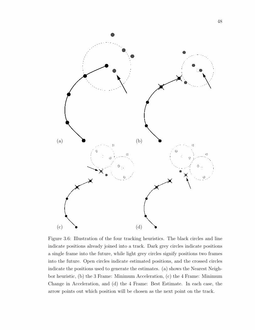
48

(a) (b)

(c) (d)

Figure 3.6: Illustration of the four tracking heuristics. The black circles and line

indicate positions already joined into a track. Dark grey circles indicate positions

a single frame into the future, while light grey circles signify positions two frames

into the future. Open circles indicate estimated positions, and the crossed circles

indicate the positions used to generate the estimates. (a) shows the Nearest Neigh-

bor heuristic, (b) the 3 Frame: Minimum Acceleration, (c) the 4 Frame: Minimum

Change in Acceleration, and (d) the 4 Frame: Best Estimate. In each case, the

arrow points out which position will be chosen as the next point on the track.

49

where Timperfect is the number of tracks the algorithm failed to produce perfectly

when compared to known tracks and Ttotal is the total number of tracks in the data

set (Chetverikov and Verestoy, 1999). In this analysis, a perfectly constructed track

may contain no spurious points and must begin at the same time as the actual data

track, although it may not have the same total length. In this way, a track that

is broken into many segments by the algorithm but contains no incorrect matches

will only count as a single correct track in the error analysis.

We have studied Etrack as a function of the parameter

ξ =∆r

∆0

, (3.24)

where ∆r is the mean distance travelled by a particle from one frame to the next

and ∆0 is the mean separation between a particle and its closest neighbor in a

single frame. This parameter is the inverse of the parameter p defined by Malik

et al. (1993). When ξ � 1, the particle seeding density is low and/or the particles

move slowly from frame to frame. In this limit, tracking is not difficult, and most

algorithms are expected to perform well. As ξ approaches unity, however, the

particle density is high and/or particles move large distance between frames, and

tracking becomes very difficult. Experiments, however, will tend to lie in this limit,

since a higher particle density increases the data rate of the LPT system and low

camera framerates, corresponding usually to lower-priced cameras or those with

higher spatial resolution, produce larger frame-to-frame motion.

The algorithms were tested using tracks generated by fully 3D direction numer-

ical simulation (DNS) of the Navier-Stokes equations provided by Lance Collins

at Cornell (Collins, 2003). The DNS was carried out at a Reynolds number of

Rλ = 52 in a 2π × 2π × 2π box with periodic boundary conditions. Despite this

low Reynolds number, the individual particles undergo chaotic motion and are not

50

trivial to track.

∆r was fixed in the DNS, and so to vary ξ we varied ∆0. To accomplish this,

we simply changed the size of the periodic box. When a track left the box, it was

cut and the remaining portion of the track was wrapped back into the box as a

new track. All of these sub-tracks were considered to begin at time zero, increasing

the initial particle density and therefore ξ. This technique also simulates the effect

of particles leaving the measurement volume, though no new particles enter the

volume. Because of this, ξ changes over time. Since Etrack measures the number of

tracks generated with no mistakes starting at time zero, the initial, largest value

of ξ defines the difficulty of the problem.

For the test of the tracking algorithms, simulated images were not created;

instead, the exact fluid particle positions calculated in the DNS were fed to the al-

gorithms. The results of our tests of tracking algorithms are therefore independent

of the particle center finding method chosen.

The results of testing the eight tracking algorithms are shown in Fig. 3.7. The

4BE algorithm with no conflict breaking clearly performed better than all other

algorithms tested, making no mistakes at all for ξ < 0.04. Interestingly, when the

Munkres algorithm was used in conjunction with the 4BE algorithm, its perfor-

mance was the worst of the eight algorithms.

Figure 3.7 also shows a dramatic difference between the 4BE and 4MA algo-

rithms, despite their similarity. This difference in accuracy may be attributed to

the 4MA algorithm’s estimation of the third derivative in order to select the proper

next particle position. With the limited time resolution in these simulations and

in any real LPT experiment, the third derivative is very difficult to distinguish

from noise, especially with no averaging. Because of the this, the 4MA tracking

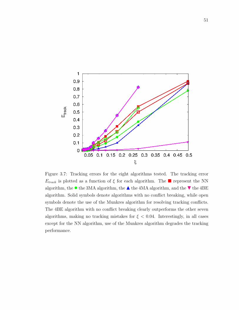
51

Figure 3.7: Tracking errors for the eight algorithms tested. The tracking error

Etrack is plotted as a function of ξ for each algorithm. The � represent the NN

algorithm, the • the 3MA algorithm, theN the 4MA algorithm, and theH the 4BE

algorithm. Solid symbols denote algorithms with no conflict breaking, while open

symbols denote the use of the Munkres algorithm for resolving tracking conflicts.

The 4BE algorithm with no conflict breaking clearly outperforms the other seven

algorithms, making no tracking mistakes for ξ < 0.04. Interestingly, in all cases

except for the NN algorithm, use of the Munkres algorithm degrades the tracking

performance.

52

heuristic is unreliable, especially for high values of ξ.

It is also apparent from Fig. 3.7 that the use of the Munkres algorithm does not,

in general, enhance the performance of a tracking algorithm. Except for the NN

algorithm, conflict breaking with the Munkres algorithm degrades the performance

of each algorithm. This suggests that when a tracking conflict occurs, it is highly

unlikely that a resolution algorithm will pick the correct position, and it is wisest

simply to halt the conflicting tracks.

On the basis of this analysis, we have chosen to use the 4BE algorithm with no

conflict breaking in our experiments. In addition, we have implemented a system

to handle the possible loss of a particle for a few frames. This loss may occur due to

occlusion of the particle, or possibly a tracking conflict. To handle this situation,

we simply extrapolate tracks when they terminate for a few frames with estimated

positions, hoping to find a continuation of the track. If such a continuation is not

found within a set number of frames, the track is fully terminated and the estimate

points are dropped.

3.2 Time Derivatives

3.2.1 Calculation

After processing the raw movies, our data is in the form of particle tracks. These

tracks can then be used to calculate many different turbulence statistics. The

statistics of interest often involve velocity or acceleration. We must, therefore, cal-

culate time derivatives from our track data. Simple finite differences, however, are

not sufficient for differentiating the tracks, even though our temporal resolution is

high. Such simple methods are easily contaminated by errors in the determination

53

of the track positions. Instead, we use a more robust method for numerical differ-

entiation. We convolve the measured particle tracks with a Gaussian smoothing

and differentiating filter, as described by Mordant et al. (2004a). This filter uses a

weighted average of many points to calculate time derivatives, reducing the effect

of noise.

The Gaussian kernel is given by

kn(τ) =dn

dτn

[1√πw

exp

(−τ 2

w2

)], (3.25)

where n is the order of the derivative we wish to calculate. The derivative of the

position is then given by

dn

dtnx(t) =

∫ ∞−∞

x(t− τ)kn(τ)dτ, (3.26)

where x denotes the noisy measured data. Integrating by parts n times, the deriva-

tive in eq. (3.25) can by passed from the Gaussian to the noisy position. The surface

term from each integration by parts vanishes since the Gaussian goes to zero at in-

finity. Our measured tracks, however, are not infinitely long. If we apply eq. (3.26)

blindly, then, we would pick up a nonzero surface term since we cannot integrate

out to infinity. Instead, we truncate and renormalize the kernel before convolution

with the measured positions. This truncation process also allows us to the set the

number of points we wish to include in the calculation of the derivative.

To illustrate this process, let us consider the velocity kernel. After truncation

and renormalization, we have

kv(τ) = Avτ exp

(−τ 2

w2

)+Bv, (3.27)

where we have absorbed the 1/(√πw) in eq. (3.25) into Av. We now restrict the

convolution to lie between T and −T , where generally (2T+1) ≈ τη. For simplicity,

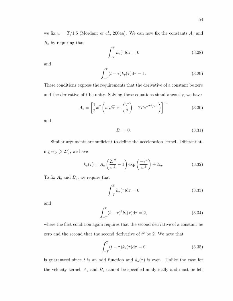
54

we fix w = T/1.5 (Mordant et al., 2004a). We can now fix the constants Av and

Bv by requiring that ∫ T

−Tkv(τ)dτ = 0 (3.28)

and ∫ T

−T(t− τ)kv(τ)dτ = 1. (3.29)

These conditions express the requirements that the derivative of a constant be zero

and the derivative of t be unity. Solving these equations simultaneously, we have

Av =

[1

2w2

(w√π erf

(T

2

)− 2Te−T

2/w2

)]−1

(3.30)

and

Bv = 0. (3.31)

Similar arguments are sufficient to define the acceleration kernel. Differentiat-

ing eq. (3.27), we have

ka(τ) = Aa

(2τ 2

w2− 1

)exp

(−τ 2

w2

)+Ba. (3.32)

To fix Aa and Ba, we require that∫ T

−Tka(τ)dτ = 0 (3.33)

and ∫ T

−T(t− τ)2ka(τ)dτ = 2, (3.34)

where the first condition again requires that the second derivative of a constant be

zero and the second that the second derivative of t2 be 2. We note that∫ T

−T(t− τ)ka(τ)dτ = 0 (3.35)

is guaranteed since t is an odd function and ka(τ) is even. Unlike the case for

the velocity kernel, Aa and Ba cannot be specified analytically and must be left

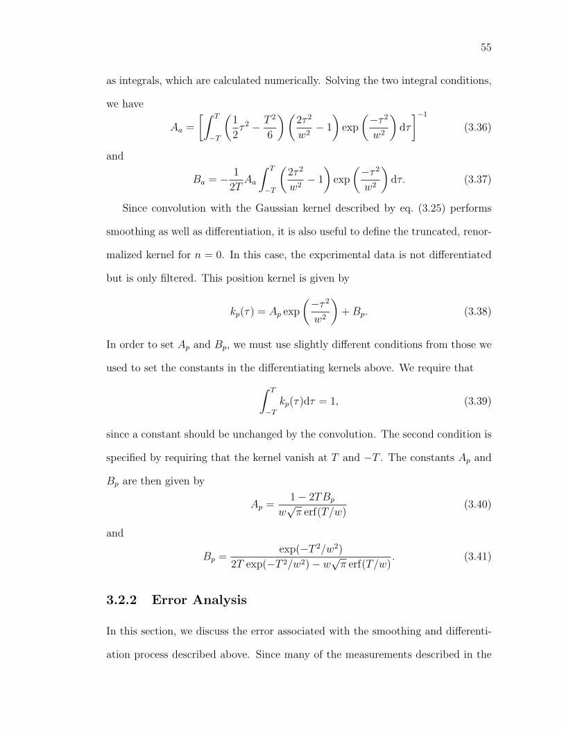
55

as integrals, which are calculated numerically. Solving the two integral conditions,

we have

Aa =

[∫ T

−T

(1

2τ 2 − T 2

6

)(2τ 2

w2− 1

)exp

(−τ 2

w2

)dτ

]−1

(3.36)

and

Ba = − 1

2TAa

∫ T

−T

(2τ 2

w2− 1

)exp

(−τ 2

w2

)dτ. (3.37)

Since convolution with the Gaussian kernel described by eq. (3.25) performs

smoothing as well as differentiation, it is also useful to define the truncated, renor-

malized kernel for n = 0. In this case, the experimental data is not differentiated

but is only filtered. This position kernel is given by

kp(τ) = Ap exp

(−τ 2

w2

)+Bp. (3.38)

In order to set Ap and Bp, we must use slightly different conditions from those we

used to set the constants in the differentiating kernels above. We require that∫ T

−Tkp(τ)dτ = 1, (3.39)

since a constant should be unchanged by the convolution. The second condition is

specified by requiring that the kernel vanish at T and −T . The constants Ap and

Bp are then given by

Ap =1− 2TBp

w√π erf(T/w)

(3.40)

and

Bp =exp(−T 2/w2)

2T exp(−T 2/w2)− w√π erf(T/w)

. (3.41)

3.2.2 Error Analysis

In this section, we discuss the error associated with the smoothing and differenti-

ation process described above. Since many of the measurements described in the

56

present work are concerned with the turbulent velocity, we will present an analysis

of the error associated with the velocity kernel; errors associated with the other

kernels are similarly defined. We note that in this section we shall consider all

times to be measured in frames and therefore to be dimensionless.

Let us continue to denote measured values that may contain noise with tildes.

As discussed above, the velocity is defined by

u(t) =

∫ T

−Tkv(τ)x(t+ τ)dτ, (3.42)

where

x(t) = x(t) + εx(t). (3.43)

Here, x(t) is the true position of the particle and εx is the error in this measurement.

We can then rewrite the measured velocity as

u(t) =

∫ T

−Tkv(τ)x(t+ τ)dτ +

∫ T

−Tkv(τ)εx(t+ τ)dτ. (3.44)

The first term in this expression can be written as the sum of the true velocity

u(t) and an error associated with the filtering process, ξf (T,w). The second term

is the propagation of the error in the position measurement through the velocity

kernel, ξx(T,w). By fixing w = T/1.5, ξf and ξx are functions only of the filter

length T .

Let us first consider the case of ξx(T ) = 0. The variance of the measured

velocity is then given by

〈u(t)2〉 =

⟨∫ T

−Tdτkv(τ)x(t+ τ)

∫ T

−Tdτ ′kv(τ

′)x(t+ τ ′)

⟩. (3.45)

57

Figure 3.8: Relative error due to the velocity kernel with no position noise, calcu-

lated from DNS data.

We can write

u(t) =

∫ T

−Tdτkv(τ)x(t+ τ)

=

∫ T

−Tdτkv(τ)

[x(t) +

∫ t+τ

t

dt′u(t′)

]=

∫ T

−Tdτkv(τ)

∫ t+τ

t

dt′u(t′), (3.46)

since x(t) is a constant and, by definition, the convolution of the velocity kernel

with a constant vanishes. Therefore, we have

〈u(t)2〉 =

∫ T

−Tdτ

∫ T

−Tdτ ′kv(τ)kv(τ

′)

∫ t+τ

t

dt′∫ t+τ ′

t

dt′′〈u(t′)u(t′′)〉. (3.47)

The only unknown quantity in this expression is the two-time velocity correlation

function R(t′− t′′) = 〈u(t′)u(t′′)〉. The exact form of this function, however, is not

known.

To investigate the magnitude of this effect, we have turned again to the DNS

58

data provided by Lance Collins (Collins, 2003) with no added noise. In Fig. 3.8,

we plot the relative error (〈u2〉1/2 − 〈u2〉1/2)/〈u2〉1/2 as a function of T . Since this

error is less than 1% for T < 70, we consider the error purely associated with the

convolution process to be negligible.

Let us consider now the variance of ξx(T ), given by

〈ξx(T )2〉 =

∫ T

−Tdτ

∫ T

−Tdτ ′kv(τ)kv(τ

′)〈εx(t+ τ)εx(t+ τ ′)〉. (3.48)

We cannot calculate this error without some assumptions. Let us assume that the

position error is δ-correlated in time and stationary, so that

〈εx(t+ τ)εx(t+ τ ′)〉 = 〈ε2x〉δ(τ − τ ′). (3.49)

This assumption is not truly realistic, since the position error will be correlated

while the particle center moves within a single camera pixel. In order to com-

pensate for this under-estimation of the error, we take 〈ε2x〉1/2 = 0.1 pixels, which

is probably an overestimate of the position uncertainty. With the assumption of

δ-correlation, eq. (3.48) is tractable, and we have that

〈ξx(T )2〉 = 〈ε2x〉2 exp(T 2/w2)

w2 (−2T + w√π exp(T 2/w2) erf(T/w))

. (3.50)

With w = T/1.5, this expression reduces to

〈ξx(T )2〉 =1.95〈ε2x〉T 3

. (3.51)

This error is, in general, not negligible, and is reflected by error bars on our velocity

statistics.

3.3 Apparatus

Figure 3.9 shows a sketch of the experimental system used to generate and measure

turbulence. In general, a Lagrangian particle tracking system consists of a flow

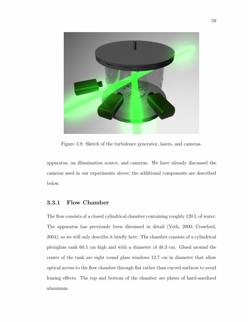
59

Figure 3.9: Sketch of the turbulence generator, lasers, and cameras.

apparatus, an illumination source, and cameras. We have already discussed the

cameras used in our experiments above; the additional components are described

below.

3.3.1 Flow Chamber

The flow consists of a closed cylindrical chamber containing roughly 120 L of water.

The apparatus has previously been discussed in detail (Voth, 2000; Crawford,

2004), so we will only describe it briefly here. The chamber consists of a cylindrical

plexiglass tank 60.5 cm high and with a diameter of 48.3 cm. Glued around the

center of the tank are eight round glass windows 12.7 cm in diameter that allow

optical access to the flow chamber through flat rather than curved surfaces to avoid

lensing effects. The top and bottom of the chamber are plates of hard-anodized

aluminum.

60

Figure 3.10: Decomposition of the large-scale flow into a pumping mode (top) and

a shearing mode (bottom).

61

Figure 3.11: Sketch of the total mean flow pattern in the flow chamber.

Turbulence is generated by the counter-rotation of two baffled disks. This type

of flow, known as a von Karman swirling flow (Zandbergen and Dijkstra, 1987),

has become increasingly popular in turbulence research in the past few decades

despite its nontrivial large-scale mean flow because it can generate high Reynolds

numbers in a small laboratory space. The large-scale flow is axisymmetric, and can

be decomposed into a pumping mode and a shearing mode, as shown in Figs. 3.10

and 3.11. The disks themselves are 20.3 cm in diameter and have a depth of 4.3

cm. Each contains twelve straight vanes so that the flow is forced inertially. Each

disk is surrounded by a plexiglass shield (not shown; see Voth (2000) or Crawford

(2004)) that breaks up any large-scale circulation and confines the bulk of the

turbulence to the center of the tank. The disks are driven by 0.9 kW DC motors

with rotation frequencies controlled through a feedback loop. A channel is cut

inside the top and bottom aluminum plates and cooling water is pumped through

62

in order to control the temperature of the water in the apparatus. The water in

the apparatus may be cleaned by pumping it through a filtering loop. A second

recirculation loop may be used to pump out bubbles and air from the apparatus

or to introduce the tracer particles.

3.3.2 Illumination

As noted above, the Phantom v7.1 cameras used in the experiments presented

here record images at a maximum rate of 27,000 frames per second at a resolution

of 256 × 256 pixels. The exposure time of each frame is therefore very short,

with a minimum of 37 µs. In order to illuminate the tracer particles, therefore,

a very intense light source must be used. When using multiple cameras, it is

also advantageous to use a pulsed light source, since pulsing obviates the need for

exact camera synchronization: the cameras will only record particle images when

the light source is on, and therefore all the cameras will record images at exactly

the same instant.

To these ends, we use Q-switched Nd:YAG solid state lasers for illumination,

frequency-doubled with a KTP crystal to provide green light at 532 nm. These

lasers are designed for both high power and high pulse rates. Three such lasers

were used in these experiments, one pumped with flashlamps and two pumped by

diode arrays. To increase the output power, each laser used two Nd:YAG rods in

series in the laser cavity.

The flashlamp laser can be run from 30 kHz to 70 kHz, with typical pulse

widths of ∼ 300 ns and peak power of ∼ 60 W. The diode pumped lasers can be

operated from 10 kHz to 120 kHz with pulse widths of ∼ 120 ns and peak power

of ∼ 90 W.

63

Care is taken in each experiment to put the cameras in the forward scattering

direction in order to maximize the amount of scattered light collected.

3.3.3 Tracer Particles

In an ideal Lagrangian particle tracking experiment, the particles used would be

true passive tracers and would behave exactly as fluid elements. Real particles,

however, have finite size and may also have a density different from that of the

carrier fluid. Because of these factors, the inertia of the particles will impair their

ability to follow the fluid flow exactly.

The importance of the particle inertia is measured by the Stokes number St,

defined as the ratio of the particle response time τp to the Kolmogorov time of

the flow τη. The Stokes number is, unfortunately, difficult to define, in great part

because it is difficult to write the equation of motion of a spherical particle in a

fluid, even at low Reynolds number. One such form is given by Shaw (2003) as

ρpVpv =6πµa(u− v) +1

2ρfVp(u− v) + 6a2√πρfµ

∫ t

0

u(t′)− v(t′)√t− t′

dt′

+ ρpVpg + ρfVpu− ρfVpg, (3.52)

where ρp and ρf are the particle and fluid densities, respectively, Vp is the volume of

the particle, a is the particle diameter, v and u are the particle and fluid velocities,

respectively, and g is the acceleration due to gravity. The terms on the right-hand

side of this expression are, in order, Stokes drag, the “added mass” due to the

acceleration of the fluid, the Basset “history” force, gravity, the fluid shear stress,

and buoyancy. We note that there is no general agreement on this form of the

equation of motion, and a different form is given by Voth (2000).

In eq. (3.52), we can neglect the gravitational effects, since they are small

64

compared with the turbulent accelerations. In the frame of reference of the particle

where v = 0, we further assume that v ∼ u ∼ u/τp. We also neglect the Basset

history force. We therefore have that

τp =1

18

ρp − ρfρf

d2

ν. (3.53)

The Stokes number can then be written as

St =1

τη

(1

18

ρp − ρfρf

d2

ν

)=

1

18

ρp − ρfρf

(d

η

)2

. (3.54)

In our experiments, we have primarily used transparent polystyrene micro-

spheres with a diameter of 25 µm, manufactured by Duke Scientific Corporation.

These microspheres have a density 1.06 times that of water, and their Stokes num-

bers are shown as a function of Reynolds number in Tabs. 3.2 and 3.3. We have

also experimented with 33 µm polystyrene microspheres containing a fluorescent

dye that absorbs light at the frequency produced by our Nd:YAG lasers and emits

in the red. These fluorescent particles have the advantage that the laser light may

be optically filtered removing any stray reflections from the camera images. In

addition, the scattering angle between the lasers and the cameras becomes unim-

portant since the fluorescent particles emit light isotropically.

3.3.4 Data Acquisition and Processing

As shown above in Table 3.1, the Phantom v7.1 cameras can take images at a

rate of up to 27,000 pictures per second at a resolution of 256× 256 pixels. Each

pixel stores eight bits of information. With these parameters, then, each camera

produces approximately 1.65 gigabytes of information every second. Since we use

three cameras in order to avoid problems of tracer particle overlap, as shown in

65

Fig. 3.9, our experimental system records just under 5 GB of information every

second.

These data rates are too high for the cameras to stream the images to disk

using current technology. Each camera, therefore, has an internal 4 GB buffer, of

which approximately 2.6 GB is available for storing pixel values, the rest being

used for overhead. The cameras can then transfer the contents of their internal

buffer over gigabit ethernet.

In order to manage and process the large amounts of data produced by this

experiment, we use a 16 node, 32-processor Pentium 4 Xeon-based computer cluster

with approximately 6 TB of disk space. During a data run, the cameras record

movies with typical lengths of one to two eddy turnover times and then transfer the

data to the cluster for processing. Since the tracking algorithms discussed above do

not lend themselves well to parallelization, the movies are transferred to multiple

nodes in sequence. Once the cameras finish transferring one set of three movies,

which typically takes about five minutes, they record the next image sequence.

By transferring the movies to the local drives of the individual nodes of the

cluster, we eliminate the potential bottleneck that could occur should multiple

nodes attempt to access the central data storage at the same time. Once a node

has finished processing a set of movies, it transfers a binary file of the calculated

particle tracks to the central data storage. The raw movies themselves are not

stored, due to space limitations. This entire data acquisition process is completely

automated, with no human control needed during the actual data run.

Once the tracks have been calculated, they are processed using specialized

software written in C++ and turbulence statistics are computed.

66

3.4 Camera Calibration

Figure 3.12 shows a single frame from each of the three cameras used in our exper-

iments. These images are fed to the computers, and the 1D Gaussian Estimator

described above is used to find the centers of the particle images in image space.

For the stereomatching and subsequent particle tracking, however, we must know

the coordinates of the particle centers in real space. We construct this mapping

using a camera calibration method developed by Tsai (1987).

Let us define the laboratory coordinates of a particle as xw, commonly called

world coordinates in machine vision. These coordinates can be mapped into the

reference frame of the camera with a rotation and a translation, given byxc

yc

zc

=

R11 R12 R13

R21 R22 R23

R31 R32 R33

xw

yw

zw

+

Tx

Ty

Tz

, (3.55)

where xc are the particle coordinates in camera space. We note that in our im-

plementation of this model we combine the rotation and the translation using ho-

mogeneous coordinates (see, e.g., Rogers and Adams (1990) for a discussion of the

properties of homogeneous coordinates). Here, however, we present the calibration

model in standard three-dimensional coordinates.

Assuming a pinhole camera with an effective focal length of feff , we can write

the perspective projection of the camera-space coordinates xc onto the ideal de-

tector coordinates xu as xu

yu

=feffzc

xc

yc

. (3.56)

Any real camera and lens system, however, will introduce some distortion, and so

67

the measured coordinates xd on the detector will be xd

yd

= (1 + k1r2 + k2r

4 + . . .)

xu

yu

, (3.57)

where r2 = x2d+y2

d. We follow Tsai (1987) in assuming that the distortion is purely

radial and that keeping only k1 is sufficient. Assuming no tangential distortion also

allows a significant simplification of the model, which Tsai (1987) refers to as the

Radial Alignment Constraint (RAC). If there is no tangential distortion, then the

distorted and ideal positions of a particle image on the detector must lie on a

line that passes through the center of the image. This condition requires that

xu × xd = 0. The final coordinate system we introduce allows a slight difference

between the horizontal and vertical spacing of the physical pixels on the detector.

We define xp

yp

=

sxxd

yd

, (3.58)

where sx is a scale factor that should, ideally, be unity if the physical detector is

ideal. Calibrating sx is then a good check on the quality of the calibration.

The calibration model as described above requires the specification of nine

parameters: three from the rotation matrix (since it is orthogonal and can be

parametrized by the Euler angles), three from the translation vector, the effective

focal length feff , the distortion coefficient k1, and sx. To gather data to set these

parameters, we have constructed a calibration mask by printing dots of a known

size onto a transparent mylar sheet with a laser printer. The dot pattern was

then sealed between two panes of glass and mounted inside the flow chamber on

a micrometer stage. Concurrent images of the calibration mask from each of the

three cameras are shown in Fig. 3.13. Since the spacing between the dots was

known and the position of the mask in the flow chamber could be measured with

68

the micrometer, imaging the mask at different positions provided a set of known

3D world coordinates paired with their corresponding detector coordinates.

Tsai (1987) presented a method for determining most of the calibration model

parameters using only linear least-squares fits. The RAC can be written as

1

sxxp (R21xw +R22yw +R23zw + Ty) = yp (R11xw +R12yw +R13zw + Tx) . (3.59)

This relation can in turn be expressed as a set of seven linear equations, namely

(−xpxw −xpyw −xpzw ypxw ypyw ypzw yp

)

T−1y R21

T−1y R22

T−1y R23

T−1y sxR11

T−1y sxR12

T−1y sxR13

T−1y sxTx

= xp.

(3.60)

By fitting these equations to the measured data from the calibration mask, the

total rotation matrix, Tx, Ty, and sx may be determined. Equation (3.57) may

then be solved iteratively for the remaining three parameters, after obtaining an

initial approximation of feff and Tz by setting k1 to zero and again performing a

least-squares fit.

Once the calibration parameters have been determined, the model can be used

to translate the measured coordinates of the tracer particle centers on the detectors

to real, laboratory-space coordinates.

69

Fig

ure

3.12

:R

awim

ages

take

nw

ith

each

ofth

eth

ree

cam

eras

aton

ein

stan

tin

the

flow

.

70

Fig

ure

3.13

:Im

ages

ofth

eca

libra

tion

mas

kfr

omea

chof

the

thre

eca

mer

as.

71

3.5 Experimental Parameters

The analysis in the following chapters is based on a number of large data sets taken

with various experimental parameters. In this section, we present the parameters

associated with each experimental run.

The integral length scale is fixed in the apparatus, and has previously been

found to be 7.1 cm (Voth et al., 2002). The first set of experiments was conducted

in a measurement volume of approximately 2 × 2 × 2 cm3. Table 3.2 shows the

values of various parameters for these experiments. Likewise, Table 3.3 shows the

values of the experimental parameters for data taken in a volume of approximately

5 × 5 × 5 cm3. In each table, the values of the dissipation rate ε are measured,

as described in the following chapter, while the Kolmogorov scales are estimated

from simple scaling arguments.

72

Tab

le3.

2:E

xp

erim

enta

lpar

amet

ers

for

the

2×

2×

2cm

3dat

aru

ns.f

den

otes

the

rota

tion

rate

ofth

edis

ks,u′ r

isth

eR

MS

radia

lve

loci

ty,u′ z

isth

eR

MS

axia

lve

loci

ty,

FP

Sis

the

num

ber

offr

ames

per

seco

nd,

andδt

isth

eti

me

bet

wee

nfr

ames

.

Thes

edat

aw

ere

take

nw

ith

tran

spar

ent

25µ

mp

olyst

yre

ne

mic

rosp

her

es.

Dat

aSet

fRλ

u′ r

u′ z

εη

L/η

τ ηTL/τη

FP

Sδt

τ η/δt

St

(Hz)

(ms−

1)

(ms−

1)

(m2s−

3)

(µm

)(m

s)(m

s)

0502

220.

3020

00.

039

0.02

56.

53×

10−

419

236

536

.851

1000

1.00

375.

7×

10−

5

0502

163.

5069

00.

473

0.30

61.

1930

2337

0.89

717

627

000

0.03

724

2.3×

10−

3

0502

215.

0081

50.

664

0.43

03.

2423

3000

0.54

420

827

000

0.03

715

3.9×

10−

3

73

Tab

le3.

3:E

xp

erim

enta

lpar

amet

ers

for

the

5×

5×

5cm

3dat

aru

ns.f

den

otes

the

rota

tion

rate

ofth

edis

ks,u′ r

isth

eR

MS

radia

lve

loci

ty,u′ z

isth

eR

MS

axia

lve

loci

ty,

FP

Sis

the

num

ber

offr

ames

per

seco

nd,

andδt

isth

eti

me

bet

wee

nfr

ames

.

Thes

edat

aw

ere

take

nw

ith

tran

spar

ent

25µ

mp

olyst

yre

ne

mic

rosp

her

es.

Dat

aSet

fRλ

u′ r

u′ z

εη

L/η

τ ηTL/τη

FP

Sδt

τ η/δt

St

(Hz)

(ms−

1)

(ms−

1)

(m2s−

3)

(µm

)(m

s)(m

s)

0504

250.

3020

00.

039

0.02

67.

09×

10−

419

236

536

.851

1000

1.00

375.

7×

10−

5

0504

240.

4324

00.

056

0.03

82.

03×

10−

314

647

921

.361

1600

0.62

534

9.8×

10−

5

0505

090.

6229

00.

083

0.05

46.

26×

10−

311

163

012

.374

3000

0.33

337

1.7×

10−

4

0504

210.

9035

00.

121

0.08

02.

01×

10−

284

830

7.11

8850

000.

200

362.

9×

10−

4

0504

141.

2941

50.

181

0.11

66.

17×

10−

264

1090

4.12

106

9000

0.11

137

5.1×

10−

4

0504

131.

8650

00.

262

0.16

90.

196

4914

332.

3912

727

000

0.03

765

8.7×

10−

4

0504

083.

5069

00.

487

0.31

51.

2430

2337

0.89

717

627

000

0.03

724

2.3×

10−

3

0504

105.

0081

50.

669

0.44

03.

3923

3000

0.54

420

827

000

0.03

715

3.9×

10−

3

Chapter 4

Single Particle Statistics

4.1 Velocity and Acceleration

The simplest quantities to consider in turbulence are the pointwise velocity and ac-

celeration. In this section, we discuss the measurement of these quantities through

their probability density functions (PDFs) before moving on to more complex,

multipoint measurements.

The PDF of the turbulent velocity fluctuations is generally expected to be close

to Gaussian. As has become apparent in recent years, however, the PDF of the

turbulent acceleration is highly non-Gaussian, and instead has a stretched expo-

nential form (La Porta et al., 2001; Voth et al., 2002; Mordant et al., 2004a). This

extreme deviation from Guassianity suggests that the acceleration is a far more

intermittent variable than the velocity. Extreme, violent acceleration events are

far more likely in turbulence than extreme velocities, and so the acceleration is

correspondingly more difficult to measure, requiring very high spatial and tem-

poral resolution. In the present work, we have focused on the statistics of the

velocity and position; as will be seen below, the acceleration is under-resolved by

our measurement system.

Since, as shown in Section 3.2.2, spatial resolution plays a role in the accuracy

of the measured velocity and acceleration, we discuss the small and large mea-

surement volume data separately, since the two experiments have different spatial

resolution.

74

75

4.1.1 Small Measurement Volume

As shown in Section 3.3.1, our apparatus has a complex mean flow. To attempt to

account for this, when we calculate the velocity and acceleration, we first average

for long times to estimate the mean flow. This mean field is then subtracted

away from the measured Lagrangian velocity and accelerations, leaving us with

the fluctuating quantities of interest in turbulence. We note that the measured

mean accelerations are exceedingly small and are due only to noise rather than to

any true mean acceleration field.

The resulting fluctuating velocities and accelerations are not isotropic, however.

We consistently find differences in many quantities calculated in the two radial

directions (x and y) and in the axial direction (z), as has been seen before in

this apparatus (Crawford, 2004). Figure 4.1 shows the standardized PDFs of the

turbulent velocity measured in the two radial directions in the 2 × 2 × 2 cm3

measurement volume at the three different Reynolds numbers measured. The solid

lines in Fig. 4.1 are standardized Gaussians. The data for all Reynolds numbers

and for both radial components is almost perfectly Gaussian.

In contrast, we show the PDFs of the axial velocity component for the same

three Reynolds numbers in Fig. 4.2. The PDF os the axial velocity clearly has

super-Gaussian tails. This behavior is most likely due to the large-scale forcing of

our flow.

All three components of the acceleration are shown in Fig. 4.3 for all three

Reynolds numbers. The solid line shows the acceleration PDF measured by Mor-

dant et al. (2004a) in the same flow using silicon strip detectors at Rλ = 690. All

three components of the current data behave similarly and agree well with the

previously measured PDF up to roughly 15〈a2〉1/2, with the tails being somewhat

76

Figure 4.1: Radial velocity PDFs in the 2 × 2 × 2 cm3 measurement volume,

normalized by the velocity variance. The solid line is a standardized Gaussian.

Data is shown for Rλ = 200 (�), Rλ = 690 (•), and Rλ = 815 (N). Closed

symbols show the PDF of the x component of the velocity, while open symbols

show the y component. The upper plot shows the PDFs plotted on a linear scale,

while the lower plot shows the same data plotted on semilogarithmic axes.

77

Figure 4.2: Axial velocity PDFs in the 2 × 2 × 2 cm3 measurement volume, nor-

malized by the velocity variance. The solid line is a standardized Gaussian. Data

is shown for Rλ = 200 (�), Rλ = 690 (•), and Rλ = 815 (N). The upper plot

shows the PDFs plotted on a linear scale, while the lower plot shows the same data

plotted on semilogarithmic axes. Unlike the radial velocity PDFs, which are very

Gaussian, the axial velocity PDF has wider tails.

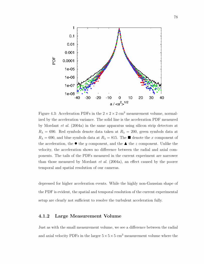
78

Figure 4.3: Acceleration PDFs in the 2× 2× 2 cm3 measurement volume, normal-

ized by the acceleration variance. The solid line is the acceleration PDF measured

by Mordant et al. (2004a) in the same apparatus using silicon strip detectors at

Rλ = 690. Red symbols denote data taken at Rλ = 200, green symbols data at

Rλ = 690, and blue symbols data at Rλ = 815. The � denote the x component of

the acceleration, the • the y component, and the N the z component. Unlike the

velocity, the acceleration shows no difference between the radial and axial com-

ponents. The tails of the PDFs measured in the current experiment are narrower

than those measured by Mordant et al. (2004a), an effect caused by the poorer

temporal and spatial resolution of our cameras.

depressed for higher acceleration events. While the highly non-Gaussian shape of

the PDF is evident, the spatial and temporal resolution of the current experimental

setup are clearly not sufficient to resolve the turbulent acceleration fully.

4.1.2 Large Measurement Volume

Just as with the small measurement volume, we see a difference between the radial

and axial velocity PDFs in the larger 5×5×5 cm3 measurement volume where the

79

spatial resolution is poorer. The standardized PDFs of one of the radial velocity

components are shown in Fig. 4.4 for Reynolds number ranging from Rλ = 200

to Rλ = 815. The agreement with the normalized Gaussian is good, though not

quite as good as for the smaller measurement volume data set, since the spatial

resolution is poorer.

The PDF of the axial velocity component is shown in Fig. 4.5 for the same

Reynolds numbers. Just as for the small measurement volume data, the axial

component is significantly less Gaussian than the radial component.

Unlike in the small measurement volume case, we see a difference between

the radial and axial acceleration PDFs, shown in Fig. 4.6. While both PDFs are

seriously under-resolved when compared with the data of Mordant et al. (2004a),

the tails of the axial PDF are systematically higher than those of the radial PDFs,

just as they were in the velocity PDF. Regardless, is it clear that only low moments

of the acceleration can by meaningfully measured with the large measurement

volume data.

4.1.3 Biases

In any particle tracking experiment, there are a number of factors that can affect

the measured turbulence statistics. Some of these factors are purely statistical in

nature, and can be corrected by collecting more data. Some, however, are inherent

biases that cannot, in general, be corrected for.

Each particle will stay in the field of view of the cameras for a different amount

of time, and so therefore each particle track will be a different length. There are

far more short tracks than long tracks measured by our experiment, as shown in

Fig. 4.7. Statistical convergence can therefore become a problem at long times.

80

Figure 4.4: Radial velocity PDFs in the (5 cm)3 measurement volume, normalized

by the velocity variance. The solid line is a standardized Gaussian. Data is shown

for Rλ = 200 (�), Rλ = 240 (�), Rλ = 290 (◦), Rλ = 350 (•), Rλ = 415 (M),

Rλ = 500 (N), Rλ = 690 (O), and Rλ = 815 (H). Only the x component of the

velocity is shown; the y component is similar.

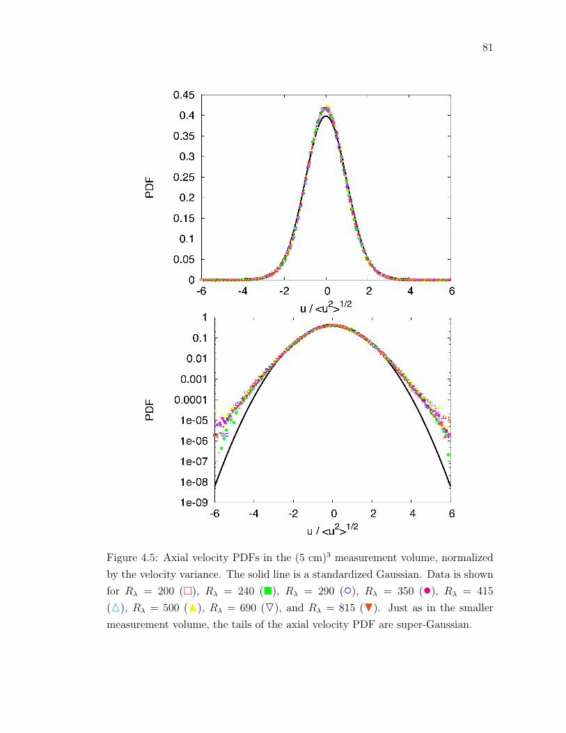
81

Figure 4.5: Axial velocity PDFs in the (5 cm)3 measurement volume, normalized

by the velocity variance. The solid line is a standardized Gaussian. Data is shown

for Rλ = 200 (�), Rλ = 240 (�), Rλ = 290 (◦), Rλ = 350 (•), Rλ = 415

(M), Rλ = 500 (N), Rλ = 690 (O), and Rλ = 815 (H). Just as in the smaller

measurement volume, the tails of the axial velocity PDF are super-Gaussian.

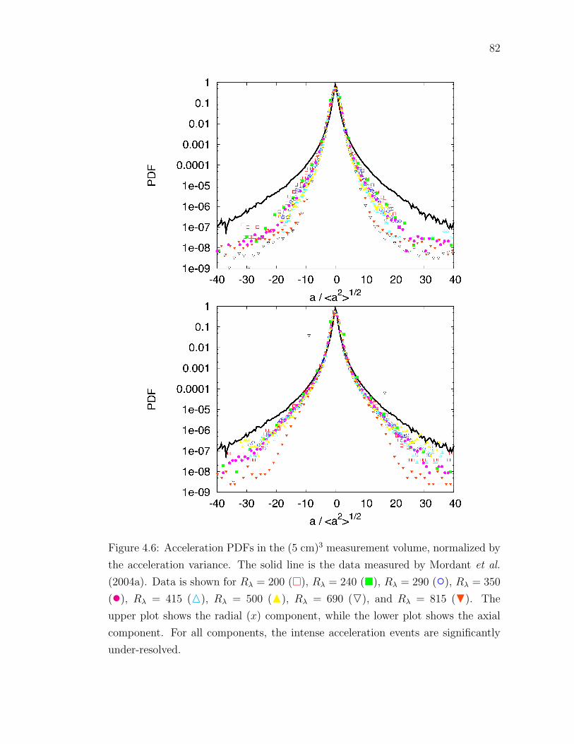
82

Figure 4.6: Acceleration PDFs in the (5 cm)3 measurement volume, normalized by

the acceleration variance. The solid line is the data measured by Mordant et al.

(2004a). Data is shown for Rλ = 200 (�), Rλ = 240 (�), Rλ = 290 (◦), Rλ = 350

(•), Rλ = 415 (M), Rλ = 500 (N), Rλ = 690 (O), and Rλ = 815 (H). The

upper plot shows the radial (x) component, while the lower plot shows the axial

component. For all components, the intense acceleration events are significantly

under-resolved.

83

Figure 4.7: Distribution of track lengths at Rλ = 690 in both the large mea-

surement volume (red symbols) and small measurement volume (green symbols).

Tracks shorter than 30 frames were not saved.

Bias errors are more subtle, and cannot be corrected simply by gathering larger

data sets. In a particle tracking experiment, biases arise due to the finite measure-

ment volume that is only a subvolume of the entire flow.

As mentioned above, few tracks remain in the measurement volume for long

times. In addition to poor statistics at long times, however, bias errors become

an issue. The particles that remain in the volume for a long time are more likely

either to be moving very slowly or to have trajectories that fold back on themselves.

These particles are therefore not representative of the full ensemble of particles in

the turbulence, and averages over these particles cannot be considered to be true

ensemble averages. More discussion of this type of bias error is given by Mordant

(2001), Crawford (2004), and Mordant et al. (2004b) in the context of the velocity

autocorrelation function. This is the primary source of bias in our experiments.

84

To avoid this error, we do not measure quantities that mix scales, such as the

autocorrelation, but instead focus on quantities that are local in scale, such as the

structure functions.

4.2 Eulerian Structure Functions

Some of the most well-studied quantities in turbulence are the moments of the Eu-

lerian velocity increments, known as the structure functions. Defining the velocity

increment as δu(r) ≡ u(x + r)− u(x), the structure function tensors are formally

defined as

DEp (r) = 〈δu(r)p〉. (4.1)

In homogeneous turbulence, the structure functions depend only on the separation

r and not the absolute positions of the two velocities.

The most important of the Eulerian structure functions are those of second

and third order with p = 2 and 3, respectively. Let us consider the second-order

structure function. Assuming isotropy and using the theory of isotropic tensors,

we can write

DEij(r) = A(r)rirj +B(r)δij, (4.2)

where A and B are functions only of the magnitude of r. Therefore, two scalar

functions are sufficient to characterize this second rank tensor fully. It is common

to choose these two functions to be the longitudinal structure function DLL(r)

where δu is parallel to the separation vector r and the transverse structure function

DNN(r) where it is orthogonal to r. Defining r as a unit vector in the direction of

85

r and ξ as a unit vector orthogonal to r, we have that

DLL(r) = DEij rirj = A(r)r2 +B(r)

DNN(r) = DEij ξiξj = B(r), (4.3)

so that

DEij(r) = [DLL(r)−DNN(r)]

rirjr2

+DNNδij. (4.4)

These two scalar functions are not independent. Using the incompressibility con-

dition, ∂Dij(r)/∂rj = 0, and so

DNN(r) = DLL(r) +1

2r

dDLL(r)

dr. (4.5)

In the inertial range, K41 gives

DLL = C2(εr)2/3, (4.6)

so that

DNN =4

3C2(εr)2/3. (4.7)

These results for the scaling of the structure functions in the inertial range are of

prime importance for experimental studies of turbulence due to the presence of the

dissipation rate ε. The dissipation rate plays a central role both in the original K41

theory and in modern studies of turbulent intermittency, and so determining ε is of

the utmost importance in any turbulence experiment. In general, the dissipation

rate is defined as

ε = 2ν〈sijsij〉, (4.8)

where

sij =1

2

(∂ui∂xj

+∂uj∂xi

)(4.9)

86

is the symmetric part of the velocity gradient tensor and is known as the rate

of strain. Direct measurement of ε requires a full determination of the velocity

gradient tensor. Such measurements are, in general, exceedingly difficult to per-

form experimentally, although they have been shown to be possible in Lagrangian

particle tracking systems at low Reynolds number (Luthi, 2002). As shown in

eqs. (4.6) and (4.7), however, measurements of the Eulerian structure functions

in the inertial range can provide an indirect measurement of the dissipation rate,

provided that the scaling constant C2 is known. The importance of the dissipation

rate coupled with the difficulty of its direct measurement have made C2 one of the

best-determined constants in turbulence, with a value of 2.13± 0.22 (Sreenivasan,

1995). Our measurements of the dissipation rate ε shown in Tables 3.2 and 3.3 are

made in this way.

Figure 4.8 shows a typical measurement of the longitudinal and transverse

Eulerian structure functions in our experiment in the small measurement volume.

The transverse structure functions have been multiplied by 3/4 in order to make

the inertial range values of the structure functions the same. In Fig. 4.9, we show

DLL and DNN compensated by C2r2/3 in order to determine the energy dissipation

rate from the plateau value.

The third-order Eulerian structure function is perhaps even more important

than the second order. By extending the results of von Karman and Howarth

(1938), Kolmogorov (1941b) was able to show directly from the Navier-Stokes

equations that in stationary, homogeneous, isotropic turbulence

DLLL(r) = −4

5εr + 6ν

∂DLL(r)

∂r, (4.10)

where DLLL(r) is the third-order longitudinal structure function, defined anal-

ogously to DLL(r) above. In the inertial range, the viscous term is negligible,

87

Figure 4.8: Second-order Eulerian velocity structure function at Rλ = 815 mea-

sured in the small measurement volume. The top plot shows DLL(r) (�) and

(3/4)DNN (•) with the horizontal coordinate scaled by the Kolmogorov length.

The bottom plot shows the same data plotted in logarithmic coordinates to show

the power law scaling. The solid line is an r2/3 power law for comparison.

88

Figure 4.9: Compensated Eulerian structure function at Rλ = 815. The longi-

tudinal (�) and transverse (•) structure functions have been scaled so that they

should show a plateau with a value of ε in the inertial range.

according to the K41 hypotheses, and so

DLLL(r) = −4

5εr. (4.11)

This result is known as the Kolmogorov 4/5 law. Unlike the second-order structure

function, where C2 must be determined experimentally by comparison with an

alternate measurement of the dissipation rate, the determination of ε from the

third-order structure function is exact.

DLLL(r) as measured at Rλ = 815 in the small measurement volume is shown in

Fig. 4.10. It is clear that the scaling range is smaller for the third-order structure

function than it is for the second-order structure functions. The compensated

third-order structure function is shown in Fig. 4.11. While the scaling range is very

short, the value of ε measured from DLLL is consistent with the values measured

from the second-order structure functions.

89

Figure 4.10: Third-order Eulerian velocity structure function at Rλ = 815 in the

small measurement volume. The solid line is a linear power law for comparison.

The scaling range for DLLL(r) is shorter than for DLL(r) and DNN(r).

4.3 Lagrangian Structure Functions

Just as the Eulerian structure functions have been instrumental in understanding

turbulence, the similarly-defined Lagrangian structure functions are a basic tool in

describing turbulence in the Lagrangian framework. To define them, let us consider

a Lagrangian velocity increment, δu(τ) = u(t + τ) − u(t). These increments are

taken along the trajectory of an individual fluid element, and are a function of

time rather than of space. Since time is not a vector, the Lagrangian structure

functions are in some sense easier to work with, since there is no separation vector

to project onto. K41 therefore says that, in the inertial range,

DLp (τ) ≡ 〈δu(τ)p〉 ∼ τ p/2, (4.12)

90

Figure 4.11: Compensated third-order Eulerian velocity structure function at Rλ =

815. While the scaling range for DLLL(r) is short, the value of ε measured from the

plateau region is consistent with that measured from the second-order structure

functions.

91

and that furthermore, these tensors should be isotropic. In the following sections,

we discuss both the second-order Lagrangian structure function in detail as well

as the scaling behavior of the high-order structure functions.

4.3.1 Second Order Structure Functions

In the inertial range, K41 states that the second-order Lagrangian structure func-

tion should scale as

DLij(τ) = 〈δui(τ)δuj(τ)〉 = C0ετδij, (4.13)

where δij is the Kronecker delta and C0 is presumed to be a universal scaling

constant for all turbulent flows, similar to C2 defined above for the second-order

Eulerian structure function. Unlike C2, however, the value of C0 is very poorly de-

termined. Lien and D’Asaro (2002) have given a review of the values of C0 reported

in the literature. These previously measured values range from 2.1 to 7.0, spanning

nearly an order of magnitude. In particular, there have only been three previous

experimental measurements of C0 (Hanna, 1981; Lien et al., 1998; Mordant et al.,

2001). All suffered from large uncertainties, and none resolved the Kolmogorov

scales. Given that C0 is an important parameter in stochastic models of turbulent

transport and dispersion (Rodean, 1991; Sawford, 1991; Weinman and Klimenko,

2000), as well as remarkably being connected both to the Richardson constant

governing the separation of fluid element pairs and to the structure functions of

the fluctuations of a scalar field passively advected by the turbulence (Sawford,

2001), a more precise determination of C0 is needed. The work presented here has

previously been reported by Ouellette, Xu, Bourgoin, and Bodenschatz (2006c).

The second-order Lagrangian structure function measured at Rλ = 815 in the

large measurement volume is shown in Fig. 4.12. As expected, the long-time be-

92

Figure 4.12: Second-order Lagrangian velocity structure function at Rλ = 815.

The bottom plot shows the same data plotted in logarithmic coordinates. The

solid line is linear in τ , corresponding to the K41 prediction for the scaling of the

structure function in the inertial range. In both plots, the � correspond to the xx

component, the • to the yy component, and the N to the axial zz component.

93

havior of the structure function reflects the large-scale anisotropy in our flow, re-

producing the difference in the RMS velocity measured in the two radial directions

and in the axial direction.

In comparison with the second-order Eulerian structure function shown in

Fig. 4.8, the inertial range seen in the Lagrangian structure function occurs at

very short times, of the order of a few τη compared with several hundred η in

the Eulerian case, and for short durations. In analogy with the typical Eulerian

definition (Anselmet et al., 1984; Frisch, 1995), we define the Lagrangian inertial

range to be the region where the second-order structure function scales linearly

with time, as predicted by K41. We note that since the K41 prediction for the

second-order Lagrangian structure function is linear in ε we expect no intermit-

tency correction, and therefore this working definition of the Lagrangian inertial

range should be valid.

The shortness of the Lagrangian inertial range is shown very clearly when we

plot the second-order structure function compensated by τε, shown in Fig. 4.13.

The most striking feature of Fig. 4.13, however, is the reflection of the large-scale

anisotropy of our flow in the small-scale behavior of the structure function. Recall

the K41 hypothesis of local isotropy: turbulence statistics are presumed to “forget”

the large-scale flow structure as energy follows the Richardson cascade down to

small scales. In many ways, the celebrated universality of turbulence statistics

rests on this assumption of local isotropy, for if small-scale statistics depend on

the detailed flow geometry at large scales, they cannot be universal for different

flows. Observation of persistent anisotropy at small scales therefore calls many of

the most basic assumptions of turbulence theory into question.

The large-scale flow in our cylindrical tank is approximately axisymmetric. Ax-

94

Figure 4.13: The xx (�), yy (•), and zz (H) components of the compensated

Lagrangian structure functions at Rλ = 815. The other symbols show the off-

diagonal components. The structure functions have been scaled by τε so that they

should show a plateau in the inertial range. The time axis has been normalized by

the Kolmogorov time. The relative magnitude of the radial and axial components

reflects the anisotropy of our large-scale flow.

95

isymmetric turbulence has been the subject of prior theoretical work (Batchelor,

1946; Chandrasekhar, 1950; Ould-Rouiss, 2001) as the simplest relaxation of the

local isotropy condition, but has unfortunately not yielded experimentally veri-

fiable predictions similar to those made by K41. The data shown in Fig. 4.13

reflects the large-scale axisymmetry very well: the off-diagonal terms of the struc-

ture function tensor are zero to within the experimental precision, and the two

radial components are equal and larger than the axial component. It is important

to note, however, that we see anisotropy only in the magnitude of the structure

function, measured by the value of C0, and not in the scaling exponent, which is

unity for both the radial and the axial components.

The lack of a long scaling region at moderate Reynolds numbers has made

prior measurements of the scaling constant C0 difficult, accounting for the dearth

of such data in the literature. Even at Rλ = 815, we do not see a very long

scaling range. We can nevertheless estimate values for C0 based on the peaks of

the compensated structure functions measured for various Reynolds numbers. As

has been seen previously (Sawford, 1991), we find a Reynolds number dependence

of C0. Our measurements of C0 are shown as a function of Reynolds number

in Fig. 4.14. The data appear to be reaching a plateau at the highest Reynolds

numbers measured, suggesting that Yeung’s (2002) estimate that true inertial range

scaling of Lagrangian quantities could be seen at Reynolds numbers of Rλ = 600−

700 is accurate.

The solid lines in Fig. 4.14 are fits of a model due to Sawford (1991) to capture

the Reynolds number dependence of C0. By fitting his second-order Lagrangian

stochastic model to low-Reynolds number DNS, Sawford (1991) proposed that

C0 =C∞0

1 + AR−1.64λ

, (4.14)

96

Figure 4.14: Measurements of C0 from the Lagrangian structure function tensor for

the xx component (�), yy component (•), and zz component (H) as a function of

Reynolds number. The zz component C0 values are smaller than those measured

for the two radial components, presumably due to the large scale axisymmetry of

our flow. C0 is observed to increase weakly with Reynolds number. The solid lines

are fits of Sawford’s model (eq. (4.14)) for the Reynolds number dependence of C0

(Sawford, 1991). We note that due to the time resolution in the Rλ = 500 data

run, we encountered large uncertainties and were not able to measure a C0 value

from the xx component. We have therefore not included the Rλ = 500 data points

in the fits of eq. (4.14).

97

where C∞0 is the asymptotic value of C0 at infinite Reynolds number. From his fits,

Sawford found that A ≈ 365, and we find A values of the same order. By fitting

this form to our C0 data, as shown in Fig. 4.14, we find that C∞0 = 6.2 ± 0.3 for

the radial structure functions and C∞0 = 5.0±0.4 for the axial structure functions.

Sawford’s (1991) scaling form for C0 appears to fit our measured data very well,

but does not predict a return to isotropy at infinite Reynolds number. Instead, the

model suggests that the anisotropy persists even as the Reynolds number increases

without bound. Further tests of this prediction must wait until a new generation of

turbulence generators is developed that can reach much higher Reynolds numbers

while retaining measurable length time scales, such as the new high-pressure SF6

wind tunnel under construction at the Max Planck Institute for Dynamics and

Self-Organization.

We have also investigated the scaling behavior of the Lagrangian velocity spec-

trum EL(ω), defined as the Fourier transform of the Lagrangian velocity auto-

correlation tensor. Since the second-order structure function is also related to

the velocity autocorrelation, an equivalence can be made between the structure

function and the spectrum. From Monin and Yaglom (1975),

DLij(τ) = 2

∫ ∞0

(1− cosωτ)ELij(ω)dω (4.15)

= C0ετδij

in the inertial range. K41 tells us that

ELij(ω) = B0εω

−2δij (4.16)

in the inertial range, and so

C0ετ = 2B0ε

∫ ∞0

1− cosωτ

ω2dω = πB0ετ, (4.17)

98

Figure 4.15: Compensated Lagrangian velocity spectra at Rλ = 690 in the x

direction (�), y direction (•), and z direction (H). By scaling the spectra by

εω−2, we expect to see a plateau in the inertial range with value B0. The frequency

axis has been scaled by the Kolmogorov frequency. As above, we note that the

difference in magnitude between the radial spectra and the axial spectrum reflects

the large scale structure of our flow.

99

so that

C0 = πB0. (4.18)

In addition to giving an independent way to measure the constant C0, it has also

been suggested that the spectrum may show better inertial range scaling behavior

than the structure function at low Reynolds numbers (Lien and D’Asaro, 2002).

Our measurement of the diagonal components of the Lagrangian spectrum at

Rλ = 690 is shown in Fig. 4.15, compensated by εω−2. The frequency axis has been

scaled by the Kolmogorov frequency; note that in the frequency domain the inertial

range corresponds to low frequencies and therefore long tracks. Such long particle

tracks are rare in our experiment, as seen in Fig. 4.7, and therefore the inertial

range in the frequency domain is under-resolved. Nevertheless, we can estimate

values of the scaling constant B0 from the peaks of the compensated spectra in the

inertial range. It is also clear from Fig. 4.15 that the anisotropy observed in our

measurements of the structure function is also present in the spectrum.

Just as we measured the scaling constant C0 as a function of Reynolds num-

ber, we have also investigated the dependence of B0 on Rλ, shown in Fig. 4.16.

Contrary to the predictions of Lien and D’Asaro (2002), we find a slightly stronger

Reynolds number dependence for the spectral scaling constant. We have again

used Sawford’s (1991) model to extrapolate asymptotic values for B0, finding that

πB∞0 = 6.3 ± 0.4 for the radial components and πB∞0 = 4.7 ± 0.4 for the axial

component. These values are in excellent agreement with the asymptotic values

estimated for C0 from the structure functions. In particular, the anisotropy again

persists for all Reynolds numbers.

Persistent anisotropy has been studied previously in Eulerian studies of ho-

mogeneous shear (Pumir and Shraiman, 1995; Pumir, 1996; Garg and Warhaft,

100

Figure 4.16: Measurements from the Lagrangian spectra for the x direction (�),

y direction (•), and z direction (H). The solid lines are again fits of eq. (4.14).

Despite the larger degree of scatter in the data, we find good agreement with C0

as calculated directly from the structure functions. Again, we have not included

the Rλ = 500 data point in the fits.

101

1998; Shen and Warhaft, 2000) and Lagrangian studies of fluid element accelera-

tion (La Porta et al., 2001; Voth et al., 2002). This anisotropy has not, however,

been observed in previous studies of C0. Indeed, only a few measurements of C0

have previously been made, as mentioned above. The experimental studies suf-

fered both from large uncertainties and from overly large Lagrangian tracers that

may have averaged out the smallest turbulence scales. Hanna (1981) measured the

Lagrangian spectra in the atmospheric boundary layer by tracking large, neutrally

buoyant balloons using radio triangulation, but acknowledged significant uncer-

tainty in the measurements. He reported a value of 4 ± 2 for πB0. Though he

measured all three diagonal components of the Lagrangian spectrum tensor, his

uncertainties were too large to find any anisotropy. Lien et al. (1998) measured

one-dimensional Lagrangian spectra using large floaters, approximately 1 m in

scale, in the oceanic boundary layer. Due to the considerable noise in their mea-

surements, they were only able to estimate that the value of πB0 lies somewhere

between 3.1 and 6.2. Since they measured only a singe component of the spectrum,

they were also unable to address questions of isotropy. Mordant et al. (2001) mea-

sured the radial Lagrangian structure function and spectrum in a one-dimensional

laboratory acoustic particle tracking experiment in a von Karman swirling flow

similar to ours. While their Lagrangian tracers were significantly smaller than

those of Hanna (1981) and Lien et al. (1998), they were still at least an order of

magnitude larger than the Kolmogorov scale. Mordant et al. (2001) measured a

maximum value of 4 for C0, though this result may be depressed by the filtering

effect of their large tracers. Lien and D’Asaro (2002) have estimated a value of 5.5

for πB0 from the spectral data of Mordant et al. (2001); since the inertial range

of the spectrum is influenced by longer particle tracks than the structure function,

102

the filtering effects may be less of an issue. Again, since Mordant et al. (2001)

measured only one component of both the structure function and the spectrum,

they were unable to address the question of isotropy.

Both the structure function and the spectrum have also been studied in DNS

(see, for example, Yeung (2001)). Since the Reynolds number must be high, how-

ever, to determine an accurate value for C0, DNS results are not conclusive. A

recent 20483 DNS study at higher Reynolds number, however, has found results

close to our measured radial values of C0 (Yeung et al., 2005). DNS, however,

though it resolves the full structure function and spectrum tensors, is usually per-

formed assuming homogeneity and isotropy, and so cannot address the persistence

of large-scale anisotropy.

The anisotropy we see in C0 and πB0 persists for all Reynolds numbers mea-

sured. Figure 4.17 shows the ratio of the radial values of C0 and πB0 to the

axial values as a function of Reynolds number. The anisotropy quantified in this

way decreases weakly with Reynolds number, but is still strongly present even at

the highest Reynolds numbers measured. This result is in contrast with measure-

ments of the anisotropy in the acceleration variance made in this same experiment

(La Porta et al., 2001; Voth et al., 2002), where the anisotropy was found to de-

crease much faster with Reynolds number. The current results show that any

return of C0 to isotropy is very slow and would require exceedingly high Reynolds

numbers to observe. This persistent anisotropy has serious implications for the

connection of isotropic theory, models, and simulations to real-world turbulent

flows. The question of how to relate such isotropic results to anisotropic flows will

be a very important topic of future research in turbulence.

103

Figure 4.17: Ratio of the C0 values measured in the radial direction and the C0

values measured in the axial direction for both the structure function (•) and the

spectrum (H). While the anisotropy decreases weakly with increasing Reynolds

number, the measurements remain far from isotropic even at the highest Reynolds

numbers measured.

104

4.3.2 Higher-Order Structure Functions

While the second-order Lagrangian structure function is of great interest since the

value of C0 is a basic parameter in many models, precise measurements of the

scaling of the higher-order Lagrangian structure functions can lead to a better

understanding of intermittency. Recall that, according to K41, the Lagrangian

structure function of order p scales in the inertial range as

DLp (τ) ≡ 〈|δu(τ)|p〉 ∼ (ετ)ζ

Lp , (4.19)

where we have now taken the absolute value of the velocity increment in order

to define the odd-order moments. K41 predicts that ζLp = p/2. But, as discussed

above, since the mean rate of energy dissipation ε is insufficient to characterize tur-

bulence, we expect deviations from the K41 prediction. This anomalous scaling is

well-studied in the Eulerian framework (Anselmet et al., 1984; Frisch, 1995; Chen

et al., 2005), but, as is usual, is not well-characterized in the Lagrangian frame-

work. Mordant et al. (2001) measured the ζLp for the first- through sixth-order

Lagrangian structure functions. No other experimental measurements have been

made, due in a large part to the inherent difficulties involved in directly record-

ing Lagrangian information. Simulations can measure Lagrangian statistics more

easily, but are limited by their low Reynolds numbers, especially since Lagrangian

statistics require higher Reynolds numbers than their Eulerian counterparts for

accurate measurement (Yeung, 2002). Nevertheless, a few such numerical stud-

ies have been performed. Biferale et al. (2004, 2005c) have studied the high-order

Lagrangian structure functions in the context of the multifractal formalism. Mazz-

itelli and Lohse (2004) have studied the Lagrangian statistics of both fluid elements

and bubbles in simulation. We here use our Lagrangian data to investigate the

105

Figure 4.18: Extended self-similarity plot of the high-order Lagrangian structure

functions at Rλ = 815. From top to bottom, the symbols correspond to the tenth-

order structure function to the first-order structure function, with the second-order

structure function omitted. The straight lines are fits to the data through which

we extracted the scaling exponents. The power laws were fit only to values of

DL2 (τ) corresponding to times between 3τη and 6τη, where DL

2 (τ) displayed a K41

scaling range with ζL2 ≈ 1.

scaling behavior of the high-order Lagrangian structure functions. These results

were previously reported by Xu, Bourgoin, Ouellette, and Bodenschatz (2006a).

It has now become common in studies of the Eulerian structure function scaling

exponents ζEp to use the extended self-similarity (ESS) ansatz first proposed by

Benzi et al. (1993). The foundation of ESS lies in Kolmogorov’s (1941b) 4/5 law.

Since Kolmogorov was able to show rigorously from the Navier-Stokes equations

that ζE3 = 1, we can write that

〈|δu(r)|p〉 ∼ rζEp ∼ 〈|δu(r)|3〉ζEp (4.20)

106

exactly, for arbitrary order p. Plotting the structure function of order p versus the

third-order structure function should therefore allow the measurement of ζEp . Let

us note that, strictly speaking, the Kolmogorov 4/5 law only applies to 〈δu(r)3〉

with no absolute value; Sreenivasan et al. (1996) have found small differences in

the scaling of 〈δu(r)3〉 and 〈|δu(r)|3〉. The difference is slight, however, and is very

difficult to observe experimentally.

The usefulness of ESS comes in the observation that imperfections in the power

law scaling of the structure functions appear to be correlated between structure

functions of different orders (Frisch, 1995). It has been suggested that this corre-

lation of the small-scale imperfections of the structure functions may be evidence

of new universal functions with the same scaling behavior in the near-dissipation

range (Sreenivasan and Bershadskii, 2005). In any case, plotting the structure

functions relative to one another often shows cleaner scaling behavior than plot-

ting the raw structure functions.

Because of its utility in the Eulerian framework, researchers have extended the

ESS technique to the Lagrangian case (Mordant et al., 2001; Biferale et al., 2004,

2005c). K41 predicts that ζL2 = 1; though this has not been proved rigorously from

the Navier-Stokes equations, deviation due to intermittency is not expected since

K41 also predicts that the second-order Lagrangian structure function is linear in

the dissipation rate (Boffetta et al., 2002). In Fig. 4.18, we plot the Lagrangian

structure functions of orders 1 through 10 measured at Rλ = 815 in the small

measurement volume experiment using ESS.

Strictly speaking, ESS can only be used to measure relative scaling exponents.

Since ζE3 = 1 exactly, in the Eulerian case the relative exponents may be simply

related to the true scaling exponents. This is not rigorously the case in the La-

107

Figure 4.19: Anomalous scaling of the structure function relative scaling expo-

nents ζLp /ζL2 measured using ESS as a function of order. The solid line shows the

K41 prediction for the scaling exponents, with ζL2 = 1. Different symbols denote

different Reynolds numbers: the � are for Rλ = 200, the • are for Rλ = 690, and

the N are for Rλ = 815. Strong departure from the K41 prediction is clear for all

Reynolds numbers investigated. Equivalent results are found without using ESS

(not shown). Moments of orders higher than 7 are not as well-converged statisti-

cally as the lower-order moments, as suggested by their larger error bars. These

high-order moments are plotted with open symbols.

108

grangian framework. To attempt to measure exponents as close to the true values

as possible, we have fit power laws to the Lagrangian structure functions only in

the region where the second-order structure function DL2 (τ) showed a K41 inertial

range so that ζL2 ≈ 1. For Rλ = 690 and Rλ = 815, we fit the structure functions

between 3τη and 6τη, and for Rλ = 200, we fit the structure functions between 2τη

and 4τη. These power law fits are shown in Fig. 4.18. The resulting relative expo-

nents ζLp /ζL2 are shown in Fig. 4.19 and are compared with the K41 prediction.The

exponents measured without using ESS are very similar. We find that the ζLp de-

viate more from the K41 prediction than their Eulerian counterparts, suggesting

that intermittency is stronger in the Lagrangian framework. Interestingly, we see

no anisotropy in the measured scaling exponents. Though we show only the radial

values in Fig. 4.19, the axial exponents are the same to within the experimental

accuracy.

There is some concern that the highest-order structure functions shown are not

fully converged statistically. To investigate the convergence, we have computed

the PDFs of the Lagrangian velocity increments for various times, as shown in

Fig. 4.20 for Rλ = 690. The pth moment of the velocity increment is converged if

the tails of δupP (δu) decrease, where P (δu) is the PDF of the velocity increments.

We show these moment PDFs in Fig. 4.21. For p > 7, the tails are noisy and do

not return to zero, and so these moments may not be fully converged. For this

reason, we plot their exponents with open symbols in Fig. 4.19.

Values of both the relative exponents are shown in Table 4.1, where they are

compared with the DNS results of Biferale et al. (2005c) and the experimental

measurements of Mordant et al. (2001). The absolute exponents are shown in Table

4.2. Our results agree within the uncertainty with those of Mordant et al. (2001);

109

Figure 4.20: PDFs of the Lagrangian velocity increments δu(τ) at Rλ = 690.

The PDFs have been offset for clarity. From top to bottom, the PDFs have been

calculated for τ = τη/5, 3τη/5, τη, 2τη, 3τη, 4τη, 8τη, and then increasing by 4τη each

up to 52τη ≈ TL/3. For short times, the PDFs have very wide tails reminiscent

of the acceleration PDF and are highly intermittent. The PDFs become more

Gaussian as the time lag between the two velocities is increased.

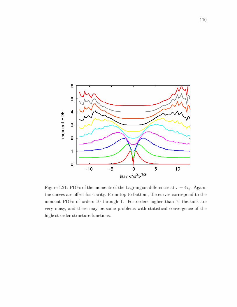
110

Figure 4.21: PDFs of the moments of the Lagrangian differences at τ = 4τη. Again,

the curves are offset for clarity. From top to bottom, the curves correspond to the

moment PDFs of orders 10 through 1. For orders higher than 7, the tails are

very noisy, and there may be some problems with statistical convergence of the

highest-order structure functions.

111

Table 4.1: Values of the relative scaling exponents measured in our experiment

using ESS. The ESS curves were fit only in the range of times where the second

order structure function displayed a K41 scaling range with exponent ζL2 ≈ 1.

For comparison, we included the values measured from the DNS of Biferale et al.

(2005c) at Rλ = 284 and the experiment of Mordant et al. (2001) at Rλ = 740.

Rλ 200 690 185 284 740

ζL1 /ζL2 0.59± 0.02 0.58± 0.05 0.58± 0.12 0.56± 0.01

ζL3 /ζL2 1.24± 0.04 1.28± 0.14 1.28± 0.30 1.34± 0.02

ζL4 /ζL2 1.35± 0.06 1.47± 0.18 1.47± 0.38 1.7± 0.05 1.56± 0.06

ζL5 /ζL2 1.39± 0.07 1.61± 0.21 1.59± 0.46 2.0± 0.05 1.73± 0.1

ζL6 /ζL2 1.40± 0.08 1.73± 0.25 1.66± 0.53 2.2± 0.07 1.8± 0.2

ζL7 /ζL2 1.39± 0.09 1.83± 0.28 1.67± 0.60

ζL8 /ζL2 1.40± 0.10 1.92± 0.32 1.65± 0.66

ζL9 /ζL2 1.42± 0.11 1.97± 0.35 1.61± 0.73

ζL10/ζL2 1.46± 0.12 1.98± 0.38 1.57± 0.80

112

Table 4.2: Values of the absolute scaling exponents measured in our experiment.

The fits were performed over the same time ranges they were for the ESS method.

Rλ 200 690 815

ζL1 0.58± 0.01 0.59± 0.04 0.58± 0.77

ζL2 0.98± 0.02 1.03± 0.07 1.01± 0.15

ζL3 1.21± 0.04 1.32± 0.11 1.30± 0.23

ζL4 1.32± 0.05 1.51± 0.15 1.49± 0.31

ζL5 1.36± 0.06 1.66± 0.18 1.61± 0.39

ζL6 1.37± 0.07 1.78± 0.22 1.68± 0.46

ζL7 1.37± 0.08 1.88± 0.26 1.69± 0.54

ζL8 1.38± 0.09 1.97± 0.29 1.67± 0.62

ζL9 1.40± 0.10 2.02± 0.33 1.62± 0.70

ζL10 1.44± 0.11 2.03± 0.37 1.58± 0.77

113

all of the experimental results, however, are significantly lower than the simulation

findings of Biferale et al. (2005c). Two parts of the analysis of Biferale et al.

(2005c) stand out as unusual. First, they fit power laws to their structure functions

between 10τη and 50τη. Not only are these times significantly longer than those

we fit to, but 50τη is longer than their reported integral time scale. The exponents

they have measured may therefore be contaminated by the large-scale forcing used

in their DNS. They report that fitting their structure functions for times shorter

that 10τη produced scaling exponents that clustered near 2 as the order of the

structure functions was increased, just as we see. In addition, Biferale et al. (2005c)

removed all particle tracks that experienced accelerations greater than 7 times the

RMS acceleration, attributing these high intensity acceleration events to particle

trapping inside intense vortical structures. By filtering out these tracks, they find

excellent agreement between their DNS and their multifractal model for the ζLp ,

which we will discuss further in the next section. We, however, believe that these

small-scale intense vortices are a fundamental part of the Lagrangian description

of turbulence and cannot be removed without drastically altering the Lagrangian

phenomenology.

We have seen from Figs. 4.18 and 4.19 that the scaling properties of the La-

grangian structure functions are anomalous when measured for time ranges where

the second-order structure function shows a K41 scaling range, which we have de-

fined to be the Lagrangian inertial range. If we blindly compensate the structure

functions by their K41 scaling laws, however, a different picture emerges. As shown

in Fig. 4.22, the structure functions do indeed show a K41 scaling range at every

order, albeit at times that become shorter as the structure function order increases.

The open circles in Fig. 4.22 show the centers of these K41 scaling ranges, which

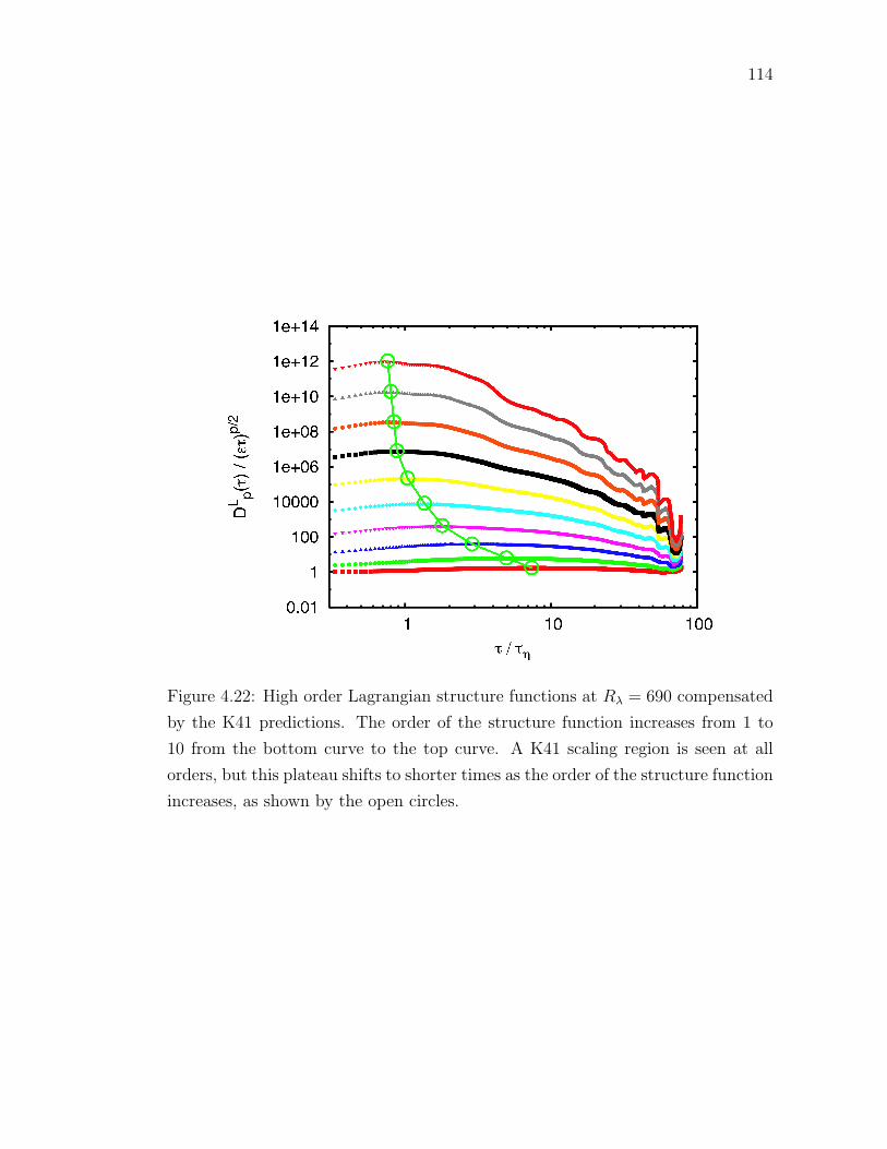
114

Figure 4.22: High order Lagrangian structure functions at Rλ = 690 compensated

by the K41 predictions. The order of the structure function increases from 1 to

10 from the bottom curve to the top curve. A K41 scaling region is seen at all

orders, but this plateau shifts to shorter times as the order of the structure function

increases, as shown by the open circles.

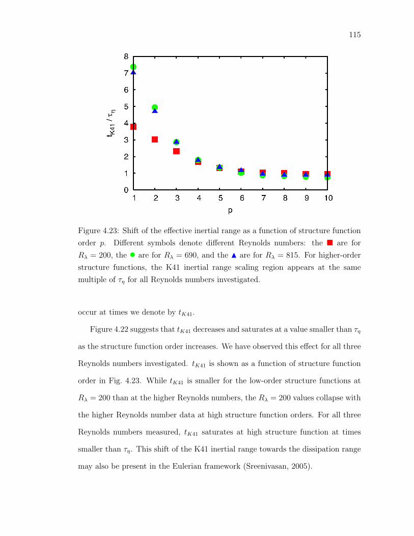
115

Figure 4.23: Shift of the effective inertial range as a function of structure function

order p. Different symbols denote different Reynolds numbers: the � are for

Rλ = 200, the • are for Rλ = 690, and the N are for Rλ = 815. For higher-order

structure functions, the K41 inertial range scaling region appears at the same

multiple of τη for all Reynolds numbers investigated.

occur at times we denote by tK41.

Figure 4.22 suggests that tK41 decreases and saturates at a value smaller than τη

as the structure function order increases. We have observed this effect for all three

Reynolds numbers investigated. tK41 is shown as a function of structure function

order in Fig. 4.23. While tK41 is smaller for the low-order structure functions at

Rλ = 200 than at the higher Reynolds numbers, the Rλ = 200 values collapse with

the higher Reynolds number data at high structure function orders. For all three

Reynolds numbers measured, tK41 saturates at high structure function at times

smaller than τη. This shift of the K41 inertial range towards the dissipation range

may also be present in the Eulerian framework (Sreenivasan, 2005).

116

4.4 Single Particle Dispersion

Having now discussed the statistics of the velocity of a single fluid element in some

detail, let us turn to position statistics. The motion of individual fluid elements

in turbulence is much more complex than what would be expected from typical

Brownian molecular diffusion. This dispersion of single fluid elements in a turbu-

lent flow is common to many applied problems outside of typical homogeneous,

isotropic turbulence studies; examples include the dispersal of marine larvae in the

ocean (Siegel et al., 2003) and the spread of plant pathogens in the atmosphere

(Brown and Hovmøller, 2002). The relative motion of fluid elements is also of great

relevance to these problems; we discuss turbulent relative dispersion in detail in

the next chapter.

Just as with the velocity statistics discussed above, we consider here not the

absolute position of a fluid particle but rather the position differences. Unfortu-

nately, however, the raw position difference x(t + τ) − x(t) is not universal, and

a Kolmogorov scaling law cannot be written for it (Monin and Yaglom, 1975).

Instead, we consider the quantity

δyi(τ) = xi(t+ τ)− [xi(t) + ui(t)τ ], (4.21)

which measures the deviation of a fluid element trajectory from a straight track

with constant velocity u(t). The usefulness of this quantity stems from the relation

(Monin and Yaglom, 1975)

δyi(τ) =

∫ τ

0

δui(t′)dt′. (4.22)

Let us consider the correlation of δyi(τ) with the Lagrangian velocity increment.

117

Using eq. (4.22), we can write that

〈δyi(τ)δuj(τ)〉 =

⟨[∫ τ

0

δui(t′)dt′

]δuj(τ)

⟩=

∫ τ

0

〈δui(t′)δuj(τ)〉dt′. (4.23)

The quantity inside the integral is nearly the Lagrangian structure function dis-

cussed above, except that the two velocity increments are taken over different

times. We can now make use of an identity proved by Monin and Yaglom (1975)

for isotropic turbulence, namely that

〈δui(t′)δuj(t′′)〉 =1

2δij[DL(t′) +DL(t′′)−DL(|t′ − t′′|)

], (4.24)

where DL(t) are the diagonal components of the second-order Lagrangian structure

function tensor. We can then write the correlation of interest as

〈δyi(τ)δuj(τ)〉 =1

2C0εδij

∫ τ

0

(t′ + τ − |t′ − τ |) dt′

=1

2C0ετ

2δij (4.25)

in the inertial range, where the last equality follows since t′ ≤ τ from the limits

of integration. This correlation thus gives us yet another way to measure the

Lagrangian structure function constant C0.

The autocorrelation of δy(τ) gives us a fourth way to measure C0. In a similar

manner as above, we can write

〈δyi(τ)δyj(τ)〉 =

∫ τ

0

dt′∫ τ

0

dt′′〈δui(t′)δuj(t′′)〉

=1

2C0εδij

∫ τ

0

dt′∫ τ

0

dt′′ (t′ + t′′ − |t′ − t′′|) . (4.26)

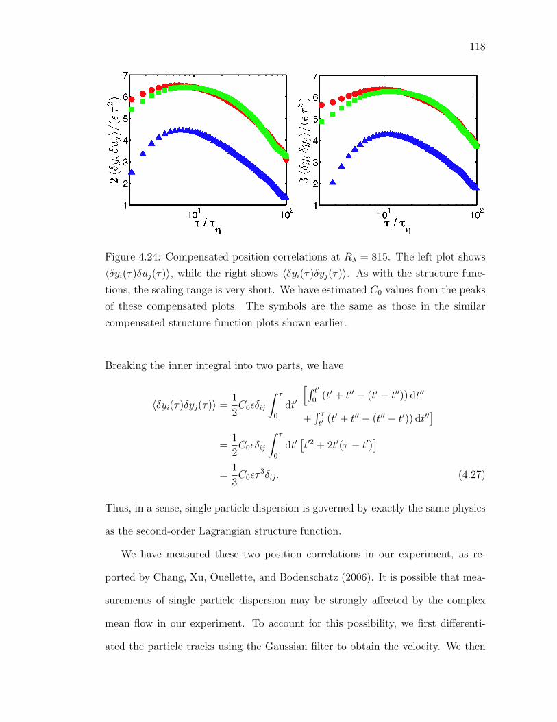
118

Figure 4.24: Compensated position correlations at Rλ = 815. The left plot shows

〈δyi(τ)δuj(τ)〉, while the right shows 〈δyi(τ)δyj(τ)〉. As with the structure func-

tions, the scaling range is very short. We have estimated C0 values from the peaks

of these compensated plots. The symbols are the same as those in the similar

compensated structure function plots shown earlier.

Breaking the inner integral into two parts, we have

〈δyi(τ)δyj(τ)〉 =1

2C0εδij

∫ τ

0

dt′

[∫ t′0

(t′ + t′′ − (t′ − t′′)) dt′′

+∫ τt′

(t′ + t′′ − (t′′ − t′)) dt′′]

=1

2C0εδij

∫ τ

0

dt′[t′2 + 2t′(τ − t′)

]=

1

3C0ετ

3δij. (4.27)

Thus, in a sense, single particle dispersion is governed by exactly the same physics

as the second-order Lagrangian structure function.

We have measured these two position correlations in our experiment, as re-

ported by Chang, Xu, Ouellette, and Bodenschatz (2006). It is possible that mea-

surements of single particle dispersion may be strongly affected by the complex

mean flow in our experiment. To account for this possibility, we first differenti-

ated the particle tracks using the Gaussian filter to obtain the velocity. We then

119

Figure 4.25: C0 measured from the position correlations as a function of Reynolds

number. On the left, we show C0 determined from 〈δyi(τ)δuj(τ)〉, while on the

right we show the C0 values from 〈δyi(τ)δyj(τ)〉. The solid lines are again fits of

Sawford’s (1991) model.

subtracted the mean velocity field, just as we did for the velocity statistics pre-

sented above. The tracks were then integrated numerically to recover the tracer

positions with the mean flow contribution removed. In Fig. 4.24, we show both

〈δyi(τ)δuj(τ)〉 and 〈δyi(τ)δyj(τ)〉 at Rλ = 815, compensated so that the peak value

will be C0. The same striking anisotropy observed in the second-order structure

function is also clearly present in the single particle dispersion data. Also, just as

with the structure function, the scaling range is very short, and so we are forced

to estimate C0 simply by taking the peak values of the compensated correlation

functions.

The measured C0 values again show a Reynolds number dependence that ap-

pears to be well-captured by Sawford’s (1991) model, as shown in Fig. 4.25. The

extrapolated values for C0 at infinite Reynolds number are consistent with the

values we found earlier for the structure function and the Lagrangian velocity

spectrum. The four measurements of C0 are summarized in Table 4.3.

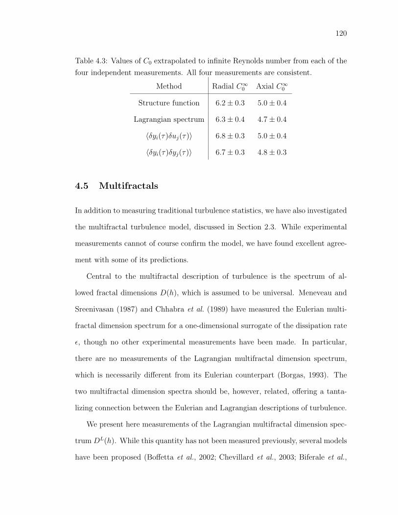
120

Table 4.3: Values of C0 extrapolated to infinite Reynolds number from each of the

four independent measurements. All four measurements are consistent.

Method Radial C∞0 Axial C∞0

Structure function 6.2± 0.3 5.0± 0.4

Lagrangian spectrum 6.3± 0.4 4.7± 0.4

〈δyi(τ)δuj(τ)〉 6.8± 0.3 5.0± 0.4

〈δyi(τ)δyj(τ)〉 6.7± 0.3 4.8± 0.3

4.5 Multifractals

In addition to measuring traditional turbulence statistics, we have also investigated

the multifractal turbulence model, discussed in Section 2.3. While experimental

measurements cannot of course confirm the model, we have found excellent agree-

ment with some of its predictions.

Central to the multifractal description of turbulence is the spectrum of al-

lowed fractal dimensions D(h), which is assumed to be universal. Meneveau and

Sreenivasan (1987) and Chhabra et al. (1989) have measured the Eulerian multi-

fractal dimension spectrum for a one-dimensional surrogate of the dissipation rate

ε, though no other experimental measurements have been made. In particular,

there are no measurements of the Lagrangian multifractal dimension spectrum,

which is necessarily different from its Eulerian counterpart (Borgas, 1993). The

two multifractal dimension spectra should be, however, related, offering a tanta-

lizing connection between the Eulerian and Lagrangian descriptions of turbulence.

We present here measurements of the Lagrangian multifractal dimension spec-

trum DL(h). While this quantity has not been measured previously, several models

have been proposed (Boffetta et al., 2002; Chevillard et al., 2003; Biferale et al.,

121

Figure 4.26: Probabilities Ph(τ) plotted as a function of τ/TL for seven values of

h in logarithmic coordinates. The curves have been offset for clarity. From top to

bottom, the data correspond to h values of 0.12, 0.25, 0.50, 0.75, 1.00, 1.25, and

1.50. The vertical lines show the region in which we fit power laws to the data.

The exponents of these power laws are given by 1−DL(h).

2004). Without experimental measurements, however, there has been no way to

differentiate between these models. The experimental results presented here were

reported previously by Xu, Ouellette, and Bodenschatz (2006b).

To measure DL(h), we have used a modified form of the probabilistic formula-

tion of the multifractal model given by Frisch (1995). Translating Frisch’s (1995)

work into the Lagrangian framework, recall that the probability Ph(τ) that a ve-

locity increment δu(τ) taken over a time τ scales as (τ/TL)h is proportional to

(τ/TL)1−DL(h). Following Frisch (1995), we define

Ph(τ) =

∫ u′(τTL

)h+∆

u′(τTL

)h−∆

Pτ (δu(τ))d[δu(τ)], (4.28)

122

where Pτ is the PDF of δu(τ), u′ is the large-scale RMS velocity, and ∆ defines a

small integration region. Formally, in the limit of infinite Reynolds number where

τη → 0, we have that

limτ→0

ln Ph(τ)

ln τ= 1−DL(h), (4.29)

In any experiment, however, the Reynolds number is finite, and we cannot take

this limit. We have therefore fit power laws to Ph(τ) in the inertial range as shown

in Fig. 4.26. The exponents from these power laws are given by 1 − DL(h), the

codimension of the Lagrangian cascade. We note that the scaling behavior of Ph(τ)

is insensitive to the integration width ∆ for ∆ ∈ [0.1u′(τ/TL)h, u′(τ/TL)h].

Our measurements of DL(h) are shown in Fig. 4.27 for three different Reynolds

numbers. The measurements agree well for all three Reynolds numbers, suggesting

that DL(h) is independent of Rλ. In addition, though we show the dimension

spectrum calculated from only a single component of δu(τ), the spectra calculated

from the other two components are identical despite the large-scale anisotropy in

our flow. Figure 4.27 also shows the predictions of several models. The left side

of our measured fractal dimension curve agrees very well with all three models,

to within the experimental accuracy. The right side of the experimental curve,

however, is very different from the model predictions, and is linear with slope

−1. We will discuss this discrepancy below, after first describing the three models

shown in Fig. 4.27 in detail.

Starting from completely Lagrangian arguments, Chevillard et al. (2003) have

proposed a simple parabolic form for the dimension spectrum, namely

DLC(h) = 1− (h− c1)2

2c2

, (4.30)

where c1 = 0.579 and c2 = 0.079 were determined from experimental measurements

of the PDF of the velocity increments. The relationship between c1 and c2 is fixed

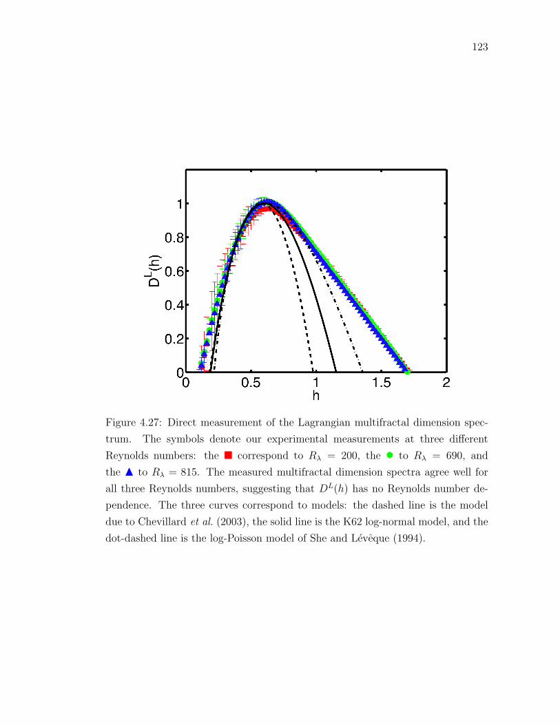
123

Figure 4.27: Direct measurement of the Lagrangian multifractal dimension spec-

trum. The symbols denote our experimental measurements at three different

Reynolds numbers: the � correspond to Rλ = 200, the • to Rλ = 690, and

the N to Rλ = 815. The measured multifractal dimension spectra agree well for

all three Reynolds numbers, suggesting that DL(h) has no Reynolds number de-

pendence. The three curves correspond to models: the dashed line is the model

due to Chevillard et al. (2003), the solid line is the K62 log-normal model, and the

dot-dashed line is the log-Poisson model of She and Leveque (1994).

124

to be c1 = 1/2 + c2 in order to force ζL2 , the scaling exponent of the second order

structure function, to be unity.

The other two models shown are Eulerian models translated into the Lagrangian

framework. In the spirit of the work done by Borgas (1993), who made a connec-

tion between the Eulerian and Lagrangian multifractal dimension spectra of the

dissipation rate by assuming that the turbulence is ergodic, Chevillard et al. (2003)

proposed that

DL(h) = −h+ (1 + h)

(DE

(h

1 + h

)− 2

), (4.31)

regardless of the form of DE(h). This equation follows from assuming a variation of

the K62 Refined Similarity Hypothesis in addition to ergodicity (Chevillard, 2004).

We here have subtracted two from DE in order to account for the difference in

the embedding dimension between 3D spatial Eulerian statistics and 1D temporal

Lagrangian statistics.

Using eq. (4.31), we have translated both the K62 log-normal model and the She

and Leveque (1994) log-Poisson model into the Lagrangian framework. While K62

was not intended to be a multifractal model (indeed, the theory of multifractals had

not yet been developed), we can use the Legendre transform relationship between

the scaling exponents of the structure functions and the multifractal dimension

spectrum in order to extract a multifractal prediction. K62 predicts that the

Eulerian structure functions scale as

〈δupr〉 ∼ rζEp ∼ r

p3− 1

2µ p

3( p3−1). (4.32)

Since

DE(h) = infh

[hp+ 3− ζEp

], (4.33)

125

we find that

DEK62(h) = 3− 9

2µ

[h−

(1

3+µ

6

)]2

. (4.34)

Using eq. (4.31), we then have

DLK62 = −h+ (1 + h)

{1− 9

2µ

[h

1 + h−(

1

3+µ

6

)]2}. (4.35)

In Fig. 4.27, we have taken µ = 1/4, a value found in experiments (Pope, 2000).

In contrast to both K62 and the Chevillard et al. (2003) model, She and Leveque

(1994) have proposed a model of the Eulerian multifractal dimension spectrum with

no free parameters. In this model, the dimension spectrum is given by

DESL(h) = 1 + b1

(h− 1

9

)− b2

(h− 1

9

)ln

(h− 1

9

), (4.36)

where

b1 = 3

(1 + ln ln 3

2

ln 32

− 1

)(4.37)

and

b2 =3

ln 32

. (4.38)

Again using eq. (4.31), we can translate this form into the Lagrangian framework,

obtaining

DLSL(h) = −h+ (1 + h)

{−1 + b1

(h

1 + h− 1

9

)−b2

(h

1 + h− 1

9

)ln

(h

1 + h− 1

9

)}. (4.39)

By comparing the structure function scaling exponents predicted by our mul-

tifractal measurements using the Legendre transform relationship

ζLp = infh

[hp+ 1−DL(h)] (4.40)

with directly measured scaling exponents, we can check for consistency in our mea-

surements. Such a comparison is shown in Fig. 4.28. Included are the same three

126

Figure 4.28: Scaling exponents ζLp of the Lagrangian structure functions as a func-

tion of order. The • denote direct measurements of the ζL(p) at Rλ = 690. The �

show the exponents extracted from our measured DL(h) data via eq. (4.40). The

two experimental measurements agree very well with each other. The curves are

models: the dashed line is again the model of Chevillard et al. (2003), the solid

curved line is the K62 log-normal model, and the dot-dashed line is the model of

She and Leveque (1994). The solid straight line shows the K41 prediction for the

ζLp .

127

models as well as the K41 prediction. Clearly, the scaling exponents computed

by taking the Legendre transform of the experimentally measured multifractal di-

mension spectrum agree very well with the directly measured Lagrangian structure

function scaling exponents. The three models agree well with our experimental re-

sults for low structure function orders, but start to deviate significantly for orders

greater than 5. This discrepancy is in part due to small differences in the value of

hmin between our measurements and the three models. Due to the finite domain

of h, eq. (4.40) implies that ζLp will change from a curved function of p to a linear

law at some p∗ where hmin minimizes the right hand side of eq. (4.40). For p > p∗,

the multifractal model predicts that ζLp = hminp + 1. Small changes in hmin can

therefore have a large impact in the predicted form of the ζLp at high orders.

Before discussing the right side of the multifractal dimension spectrum in more

detail, let us briefly discuss the proposed multifractal model of Boffetta et al.

(2002). This model, giving an expression for the ζLp based on the DE(h) of She

and Leveque (1994), is superficially different from the Lagrangian translation of

the She and Leveque (1994) model we have presented here. Boffetta et al. (2002)

begin by assuming that, to leading order,

δu(τ) ∼ δu(r), (4.41)

where δu(r) is the Eulerian velocity increment. They also assume that the char-

acteristic flow time scale at a length scale r is given by

τr ∼r

ur, (4.42)

where ur is the velocity at the scale r. Using the Eulerian multifractal formalism

as presented in Section 2.3, we then have

τr ∼r

ur∼ r

u′

( rL

)−h∼ L

u′r

L

( rL

)−h∼ TL

( rL

)1−h, (4.43)

128

so that

r

L∼(τrTL

)1/(1−h)

. (4.44)

The velocity increment then scales as

δu(τ) ∼ δu(r) ∼ ur

( rL

)3−DE(h)

∼ ur

(τrTL

) 3−DE(h)1−h

. (4.45)

We can then construct the structure function as

〈δu(τ)p〉 ∼∫h∈[hmin,hmax]

d[µ(h)]u′p( rL

)hp( τrTL

) 3−DE(h)1−h

∼∫h∈[hmin,hmax]

d[µ(h)]u′p(τrTL

)hp+3−DE(h)1−h

(4.46)

Since in the inertial range the smallest exponent will dominate the integral, we

finally have

ζLp = infh

[hp+ 3−DE(h)

1− h

]. (4.47)

Though this form looks significantly different from eq. (4.40), let us consider com-

bining eq. (4.40) with eq. (4.31). We then have

infh

[hp+ 1−DL(h)] = infh

[hp+ 1 + h− (1 + h)

(DE

(h

1 + h

)− 2

)]= inf

χ

[(χ

1− χ

)p+ 1 +

(χ

1− χ

)−(

1 +χ

1− χ

)(DE(χ)− 2

)](4.48)

= infχ

[χp+ 3−DE(χ)

1− χ

],

where we have made the change of variables χ = h/(1 + h). We therefore recover

the prediction of Boffetta et al. (2002) using the translation equation of Chevillard

et al. (2003). We prefer to treat the mapping of Chevillard et al. (2003) as more

fundamental, since it makes fewer assumptions (Chevillard, 2004; Chevillard et al.,

2005).

Let us now return to the right side of DL(h) where our experimental measure-

ments differ strongly from the three models. Just as the finite domain of h implies

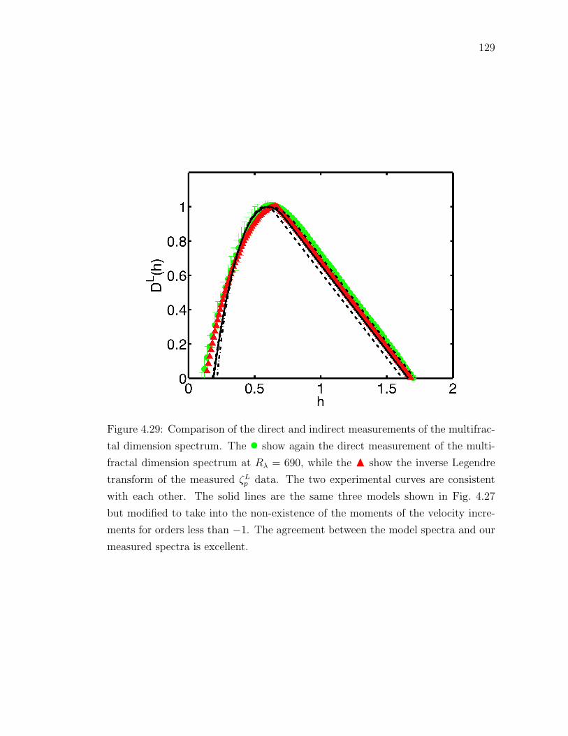
129

Figure 4.29: Comparison of the direct and indirect measurements of the multifrac-

tal dimension spectrum. The • show again the direct measurement of the multi-

fractal dimension spectrum at Rλ = 690, while the N show the inverse Legendre

transform of the measured ζLp data. The two experimental curves are consistent

with each other. The solid lines are the same three models shown in Fig. 4.27

but modified to take into the non-existence of the moments of the velocity incre-

ments for orders less than −1. The agreement between the model spectra and our

measured spectra is excellent.

130

a transition to a linear law for the ζLp , any minimum or maximum values of p would

imply a linear portion of the multifractal dimension spectrum. It is well-known

that the moments of the velocity increments do not converge for orders less than

or equal to −1 (Frisch, 1995). Therefore, pmin = −1, and DL(h) = 1 + ζL−1 − h

for p < pmin. The right side of our DL(h) is therefore explained, since it is linear

with a slope of −1. We can also take pmin into account in the three models by

using the Legendre transform relationship; these “corrected” models are shown in

Fig. 4.29. The agreement with the experimental results is remarkable. We have

also included in Fig. 4.29 the inverse Legendre transform of our directly-measured

ζLp for completeness. It too agrees very well with the directly measured multifractal

dimension spectrum.

It remains unclear how the multifractal dimension spectrum computed from the

velocity increments is related to that of the energy dissipation rate. The moments

of ε are thought to be finite at all orders, so that there will be no linear region

for the dimension spectrum computed from it. It is possible that the multifractal

dimension spectrum simply cannot be fully measured from the velocity increments.

Indeed, some researchers have claimed that wavelet transforms are needed instead

(Muzy et al., 1993). It is also possible, however, that the multifractal dimension

spectra computed from different quantities are in fact themselves different.

Chapter 5

Multiparticle Statistics

5.1 Turbulent Relative Dispersion

In the previous chapter, we have discussed the statistics of single particles in tur-

bulence. Since turbulent flows are replete with long-range correlations, however, a

full understanding of the problem cannot be gained without also investigating the

statistics of groups of particles. The simplest multiparticle problem is that of the

rate of separation of a pair of fluid elements, termed turbulent relative dispersion.

In a quiescent fluid, the spreading of two fluid elements is dominated by dif-

fusion. The fluid elements will undergo Brownian motion, and the mean-square

separation between them will grow linearly in time. Two fluid elements in a turbu-

lent flow will also experience this linear Taylor diffusion (Taylor, 1922), provided

that they are separated by a distance larger than the integral length scale. For

smaller, inertial range separations, however, the two fluid elements will separate

faster. Since this relative dispersion is closely tied to turbulent mixing (Kraichnan,

1966; Nelkin and Kerr, 1981; Sawford, 2001), the superdiffusive separation of fluid

element pairs explains why turbulent flows are so much more effective at mixing

than their laminar counterparts.

Such turbulent mixing is ubiquitous in nature (Shraiman and Siggia, 2000):

it is the basis of nearly all industrial fluid mixing processes, and it determines

the spread of pollutants or bioagents in the atmosphere (Huber et al., 2001) and

oceans (Berloff et al., 2002). Marine predator-prey systems exploit the properties of

turbulent dispersion (Jørgensen et al., 2005), and many animals use the structure

of turbulent odor plumes to locate food, predators, and mates (Balkovsky and

131

132

Shraiman, 2002; Wolf et al., 2004; Moore and Crimaldi, 2004). As with most

aspects of turbulence, passively advected scalar fields like odors, heat, or pollutants

are characterized by intense fluctuations in the local concentration relative to the

mean concentration field. These fluctuations often largely determine the dynamics

of these scalar fields. The rate of destruction of atmospheric ozone, for example,

is heavily influenced by the local concentration of the various chemical species

involved (Edouard et al., 1996), just as in many other slow chemical reactions. It

is natural to relate these concentration fluctuations to turbulent relative dispersion

(Kraichnan, 1966; Nelkin and Kerr, 1981; Sawford, 2001).

In the following sections, we discuss some of the theoretical predictions for the

scaling of turbulent relative dispersion as well as our experimental measurements.

The results of Section 5.1.3 were previously reported in Bourgoin, Ouellette, Xu,

Berg, and Bodenschatz (2006), and the results of Sections 5.1.4, 5.1.5, and 5.1.6

were reported in Ouellette, Xu, Bourgoin, and Bodenschatz (2006b).

5.1.1 The Richardson-Obukhov Law

In a turbulent flow, at scales smaller than the integral scales, pairs of fluid ele-

ments separate faster than pure Brownian motion would suggest. Once a pair of

fluid elements has separated to the integral scale, the separation will again grow

linearly. Based on physical arguments and measurements of pair separation over

a wide range of scales, Richardson (1926) suggested that the mean-square separa-

tion between two fluid elements should grow not linearly in time but rather as t3.

Subsequently, Obukhov (1941) used K41 theory to write that

〈r2〉 = gεt3, (5.1)

133

where r is the relative distance between two fluid elements. Equation (5.1) is

known as the Richardson-Obukhov law, and g is termed the Richardson constant.

Researchers have attempted to find Richardson-Obukhov scaling in experiments

(Huber et al., 2001; Ott and Mann, 2000), simulations (Yeung, 1994; Boffetta and

Sokolov, 2002a; Ishihara and Kaneda, 2002; Yeung and Borgas, 2004; Gioia et al.,

2004; Biferale et al., 2005a), and models (Sawford, 2001; Nicolleau and Yu, 2004)

for decades. No convincing evidence of the Richardson-Obukhov law, however,

has been found, and estimates of the Richardson constant span a full order of

magnitude (Sawford, 2001).

5.1.2 Batchelor’s Extension

While the Richardson-Obukhov law is the only choice consistent with K41 when the

only relevant parameter is the time of separation, Batchelor (1950) realized that a

different scaling law is possible if the initial separation r0 of the two fluid elements

remains a relevant parameter in their subsequent spreading. Let us consider the

time derivative of the mean-square separation. Using the chain rule, we can write

d

dt〈r2(t)〉 = 2〈r(t)δu(t)〉, (5.2)

where δu(t) is the relative velocity of the two fluid elements. Using the fundamental

theorem of calculus, we can then write

d

dt〈r2(t)〉 = 2

⟨[r0 +

∫ t

0

δu(t′)dt′]δu(t)

⟩= 2

{〈r0δu(t)〉+

∫ t

0

〈δu(t)δu(t′)〉dt′}. (5.3)

In his original work, Batchelor set the term 〈r0δu(t)〉 to zero, reasoning that there

should be no correlation between the initial pair separation and the relative ve-

134

locity. We, however, find that this assumption does not hold, as will be discussed

below. We therefore keep this correlation in our calculations.

We now assume that the relative velocity changes slowly in time, so that

〈δu(t)δu(t′)〉 ≈ 〈δu(0)2〉. (5.4)

This quantity in turn is exactly the same as 〈δu(r0)2〉, the trace of the second-order

Eulerian structure function. We therefore have that

d

dt〈r2(t)〉 = 2 {〈r0δu(t)〉+ [DLL(r0) + 2DNN(r0)] t}

= 2

{〈r0δu(t)〉+

11

3C2(εr0)2/3t

}. (5.5)

Therefore, when the initial separation is relevant, the relative dispersion is given

by

〈[ri(t)− r0i]2〉 =

11

3C2(εr0)2/3t2. (5.6)

This law, which we term Batchelor scaling, should hold for times of the order of

the correlation time t0 of an eddy of characteristic size r0. This time is given by

K41 as

t0 =

(r2

0

ε

)1/3

. (5.7)

When t � t0, the initial separation will no longer be a relevant parameter, and a

particle pair is expected to obey the Richardson-Obukhov law. Finally, therefore,

in turbulent relative dispersion, the mean-square separation between a pair of fluid

elements should scale as

〈[ri(t)− r0i]2〉 =

113C2(εr0)2/3t2, t� t0

gεt3, t0 � t� TL

(5.8)

Both the Batchelor t2 law and the Richardson-Obukhov t3 law should be found

in the inertial range. To distinguish these two scaling laws clearly, then, the inertial

135

range must be very large. The size of the inertial range is roughly given by the ratio

of the eddy turnover time TL to τη. Since Rλ ∼ (TL/τη), a large Reynolds number

is required to see both the Batchelor and the Richardson-Obukhov laws. Previous

experimental and numerical studies of relative dispersion have been conducted

only at low Reynolds numbers (Rλ < 300) (Yeung, 1994; Ott and Mann, 2000;

Boffetta and Sokolov, 2002a; Ishihara and Kaneda, 2002; Yeung and Borgas, 2004;

Biferale et al., 2005a) and cannot therefore be conclusive (Sawford, 2001). High

Reynolds numbers are obtained in kinematic simulations (Nicolleau and Yu, 2004),

but Thomson and Devenish (2005) have recently suggested that such models may

be ill-suited to the pair dispersion problem.

5.1.3 Experimental Results

We have measured relative dispersion from the tracer particle trajectories in the

5 × 5 × 5 cm3 volume over a range of Reynolds numbers (Bourgoin et al., 2006).

One such pair of trajectories is shown in Fig. 5.1, measured at Rλ = 690. The two

particles enter the measurement volume at the same time with an initial separation

r0 of 0.9 mm. The particles are advected by the turbulence, and have separated to

a distance of 6.3 mm by the time they leave the measurement volume. In Fig. 5.1,

the small spheres mark every other measured position of the particles and are

separated by 0.074 ms = τη/13, while the large spheres mark every 30th position

of the particles. The color of the spheres indicates the velocity of the particle.

By recording the relative separation of many such particle pairs, we have

measured the relative dispersion. In Fig. 5.2, we show our measurements of

〈[ri(t) − r0i]2〉 at Rλ = 815 with both axes normalized by the Kolmogorov scales.

Figure 5.2 shows the dispersion for fifty different bins of initial separations, 1 mm

136

Figure 5.1: A pair of measured particle trajectories at Rλ = 690. The two particles

enter the measurement volume as indicated and separate superdiffusively under the

influence of the turbulence. The small spheres mark every other measured position

of the particles, while the large spheres mark every 30th position. The color of each

sphere indicates its absolute velocity in units of m/s.

137

Figure 5.2: Evolution of the mean-square particle separation at Rλ = 815. Each

set of symbols represents a bin of initial separations 1 mm (≈ 43η) wide, ranging

from 0-1 mm to 49-50 mm. With both axes normalized by the Kolmogorov scales,

each data curve follows a power law for over two decades in time.

wide (≈ 43η) and ranging from 0-1 mm to 49-50 mm. It is clear that for each of

these initial separations, even though the largest is approximately 70% of the inte-

gral scale L, the data follows a power law for more than two decades in time. The

data, however, do not collapse for the different initial separations, suggesting that

the initial separation remains a relevant parameter and that therefore the data

cannot be following the Richardon-Obukhov law. Recalling Batchelor’s prediction

for the short-time behavior of the relative dispersion, in Fig. 5.3 we scale the same

data by (11/3)C2(εr0)2/3 and observe a nearly perfect collapse of the data for the

various initial separations. We emphasize that the dark line drawn in Fig. 5.3 is

not a fit but is rather Batchelor’s predicted power law.

If we now look closer at the agreement of our data with Batchelor’s prediction by

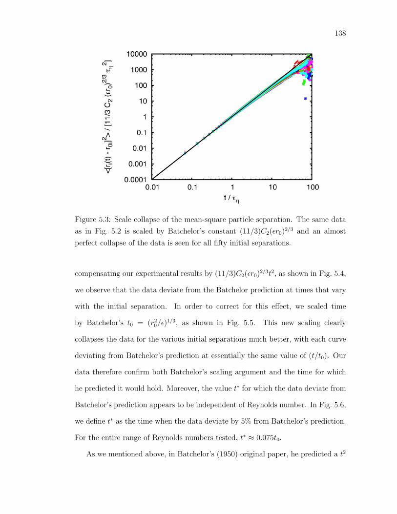
138

Figure 5.3: Scale collapse of the mean-square particle separation. The same data

as in Fig. 5.2 is scaled by Batchelor’s constant (11/3)C2(εr0)2/3 and an almost

perfect collapse of the data is seen for all fifty initial separations.

compensating our experimental results by (11/3)C2(εr0)2/3t2, as shown in Fig. 5.4,

we observe that the data deviate from the Batchelor prediction at times that vary

with the initial separation. In order to correct for this effect, we scaled time

by Batchelor’s t0 = (r20/ε)

1/3, as shown in Fig. 5.5. This new scaling clearly

collapses the data for the various initial separations much better, with each curve

deviating from Batchelor’s prediction at essentially the same value of (t/t0). Our

data therefore confirm both Batchelor’s scaling argument and the time for which

he predicted it would hold. Moreover, the value t∗ for which the data deviate from

Batchelor’s prediction appears to be independent of Reynolds number. In Fig. 5.6,

we define t∗ as the time when the data deviate by 5% from Batchelor’s prediction.

For the entire range of Reynolds numbers tested, t∗ ≈ 0.075t0.

As we mentioned above, in Batchelor’s (1950) original paper, he predicted a t2

139

Figure 5.4: Compensated mean-square particle separation. The time axis is scaled

by τη. The data for different initial separations deviate from the Batchelor predic-

tion at different times.

Figure 5.5: Compensated mean-square particle separation with time scaled by t0.

Plotted in this way, there is a scale collapse in both space and time.

140

Figure 5.6: Deviation from Batchelor’s prediction. t∗ measures the time when

the relative dispersion data deviate by more than 5% from Batchelor’s prediction.

t∗ is plotted against the initial separation for eight different Reynolds numbers.

Irrespective of Reynolds number, t∗ ≈ 0.075t0.

141

Figure 5.7: Batchelor’s original measure of relative dispersion at Rλ = 815. No

universal behavior is seen for different initial separations. The top plot shows the

raw data, while the bottom shows an attempt to collapse the data with Batchelor’s

scaling prediction.

142

law for short times for the quantity [〈r(t)2〉 − r20] rather than for 〈[ri(t) − r0i]

2〉,

shown above. When we plot this quantity, we see no universal behavior, as shown in

Fig. 5.7. This suggests that the difference between [〈r(t)2〉−r20] and 〈[ri(t)−r0i]

2〉,

namely the correlation between the initial separation and the relative velocity, is

not negligible. This non-universal behavior has also been seen in DNS studies of

relative dispersion (Biferale et al., 2005a).

As shown in Figs. 5.2-5.5, we see no Richardson-Obukhov t3 scaling for 〈[ri(t)−

r0i]2〉, nor do we see it for [〈r2(t)〉 − r2

0] or 〈r2(t)〉. It has been suggested by some

researchers, however, that 〈[ri(t)−r0i]2〉 is contaminated by the effects of larger and

smaller scales, and that different statistics are needed to observe the Richardson-

Obukhov law (Boffetta and Celani, 2000; Boffetta and Sokolov, 2002a,b; Biferale

et al., 2005a). One proposed way to search for the Richardson-Obukhov law is to

use so-called fixed scale statistics, we discuss in detail below. We have also inves-

tigated the quantity (〈r(t)2/3〉 − r2/30 ), which should dimensionally have the same

scaling behavior as 〈[ri(t)− r0i]2〉 (Falkovich, 2005). This new measure of disper-

sion, nondimensionalized by r2/30 and compensated by t/t0, is shown in Fig. 5.8.

For small initial separations for which TL/t0 is of order 10, there is a transition to

a regime consistent with t3 scaling at times of the order of t0. For larger initial

separations for which TL/t0 is smaller, however, no such transition is seen.

It is tempting to interpret this hint of t3 scaling seen in (〈r(t)2/3〉 − r2/30 ) as

evidence of the Richardson-Obukhov law. This, however, cannot be the case. If we

do not include the initial separation r0 by either subtracting it from 〈r(t)2/3〉 or by

scaling time by t0, we see no clear transition. The classical Richardson-Obukhov

law requires that the initial separation not be a relevant parameter. In addition,

the t3 power law the data appears to be approaching in Fig. 5.8 is different for

143

Figure 5.8: Alternative measure of relative dispersion at Rλ = 815. (〈r(t)2/3〉 −r

2/30 ) is plotted, nondimensionalized by r

2/30 and compensated by t/t0. For initial

separations for which TL/t0 is of order 10 (a), a transition is seen to a non-universal

t3 law at times of the order of t0, while for larger initial separations (b) no such

transition is seen.

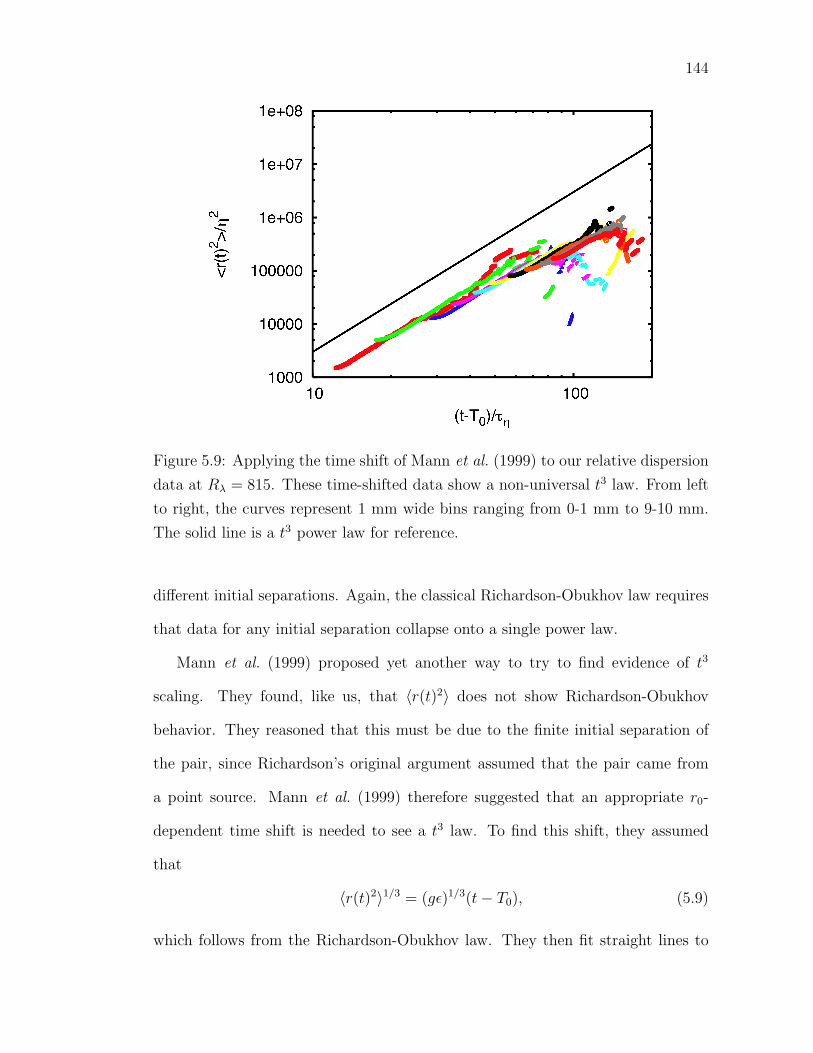
144

Figure 5.9: Applying the time shift of Mann et al. (1999) to our relative dispersion

data at Rλ = 815. These time-shifted data show a non-universal t3 law. From left

to right, the curves represent 1 mm wide bins ranging from 0-1 mm to 9-10 mm.

The solid line is a t3 power law for reference.

different initial separations. Again, the classical Richardson-Obukhov law requires

that data for any initial separation collapse onto a single power law.

Mann et al. (1999) proposed yet another way to try to find evidence of t3

scaling. They found, like us, that 〈r(t)2〉 does not show Richardson-Obukhov

behavior. They reasoned that this must be due to the finite initial separation of

the pair, since Richardson’s original argument assumed that the pair came from

a point source. Mann et al. (1999) therefore suggested that an appropriate r0-

dependent time shift is needed to see a t3 law. To find this shift, they assumed

that

〈r(t)2〉1/3 = (gε)1/3(t− T0), (5.9)

which follows from the Richardson-Obukhov law. They then fit straight lines to

145

their 〈r(t)2〉1/3 data to extract the slope and intercept, finding that T0 is, in general,

negative. This result supported their implicit assumption that r(t = T0) = 0. By

subsequently shifting their data in time by T0, Mann et al. (1999) found a t3 power

law that they identified as the Richardson-Obukhov law. When we apply their

method to our data, we also find a t3 power law, as shown in Fig. 5.9, though the

power law is not universal and is different for each initial separation. Mann et al.

(1999) were only able to look at a very small range of initial separations, and so

were not able to see the non-universality of the power law.

This method, however, has serious flaws. We can vary the process used to find

the time shift to find other power laws in the data. To find a tn power law, we

simple fit a straight line to 〈r2(t)〉1/n and fine the slope and intercept to calculate

a time shift T0. We then shift the data by T0 and obtain the desired tn law.

In Fig. 5.10, we show t4 and t5 laws obtained in this way. While they are not

perfect, they are no worse than the t3 law shown in Fig. 5.9. The reason for this

behavior is the point source assumption implicit in this method. By assuming that

at some time each particle was at the same point in space and further assuming

that the pair subsequently separated according to a tn law, the data must show a

continuation of this tn law.

Finally, we remark that since we have shown that t0 accurately characterizes

the duration of the Batchelor t2 scaling regime, observation of a true Richardson-

Obukhov scaling regime requires not only a large inertial range but also a large

scale separation between TL and t0. For the initial separations accessible in our ex-

periment, the maximum value of the ratio TL/t0 was of order 10, with no observed

Richardson-Obukhov scaling. To see a decade of Richardson-Obukhov scaling,

which would unambiguously confirm the prediction, one must therefore at mini-

146

Figure 5.10: Variations of the time shifting procedure of Mann et al. (1999) that

show a t4 power law (top) and a t5 power law (bottom) when applied to our data.

The data are the same as those shown in Fig. 5.9; the solid lines show t4 and t5

power laws for reference.

147

mum have TL/t0 ∼ 100. Using the definition of Rλ, we can write

Rλ =√

15

(TLτη

)=√

15

(TLt0

)(r0

η

)2/3

. (5.10)

The classical Richardson-Obukhov prediction is an inertial range theory. The

initial separation r0 must therefore lie in the inertial range. Following Pope (2000),

we use the common Eulerian definition of the approximate bottom of the inertial

range as about 60η. With TL/t0 ∼ 100 and r0/η ∼ 60, we can therefore estimate

that a Reynolds number of at least Rλ ≈ 6000 is required before a decade of

Richardson-Obukhov scaling can be observed.

For most flows on Earth, the Reynolds numbers are small, with Rλ typically

lower than 1000. Very turbulent atmospheric flows, such as warm clouds or the

atmospheric boundary layer (Kurien and Sreenivasan, 2001), have Rλ ∼ 104. Even

the most violent flows on Earth, such as plinian volcanic eruptions, have similar

Reynolds numbers. If we consider a pair of particles with an initial separation of

1 m in a flow with Rλ ∼ 104, such as might be found in the smokestack of an

industrial power plant, TL/t0 is only about 30, assuming typical atmospheric flow

parameters (Shaw, 2003). Even for this high-Reynolds situation, therefore, we can-

not expect the separation of the particles to be heavily influenced by Richardson-

Obukhov scaling.

5.1.4 Higher-Order Statistics

As we have shown above in Figs. 5.5 and 5.6, the mean-square pair separation

deviates from the Batchelor prediction at a universal time of roughly 0.075t0.

The dispersion slows, and as we have shown this cannot be evidence of classical

Richardson-Obukhov scaling. We are then left with only a few plausible expla-

nations for the deviation. It could be due to the influence of the large scales,

148

representing a transition to the Taylor diffusion regime, or to finite volume ef-

fects. It is also possible that the deviation is due to higher-order corrections to the

Batchelor scaling law.

Let us consider the Taylor expansion of 〈[ri(t) − r0i]2〉 about t = 0. To third

order, we have

〈[ri(t)− r0i]2〉 ≈

[〈r(t)2〉 − 2〈ri(t)〉r0i + r2

0

]∣∣t=0

+ t [2〈ri(t)δui(t)〉 − 2r0i〈δui(t)〉]|t=0

+1

2t2 [2〈δui(t)δui(t)〉+ 2〈ri(t)δai(t)〉 − 2r0i〈δai(t)〉]

∣∣∣∣t=0

+1

6t3[6〈δui(t)δai(t)〉+ 2

⟨ri(t)

∂δai(t)

∂t

⟩− 2r0i

⟨∂δai(t)

∂t

⟩]∣∣∣∣t=0

, (5.11)

where δu and δa are the relative velocity and acceleration of the particles, respec-

tively. The first two terms of this expansion drop out, leaving us with

〈[ri(t)− r0i]2〉 ≈ 〈δui(r0)δui(r0)〉t2 + 〈δui(r0)δai(r0)〉t3, (5.12)

where we have made use of the relation δu(t = 0) = δu(r0). The t2 term is exactly

the Batchelor prediction we derived above. The t3 term, however, involves the

trace of the Eulerian mixed velocity-acceleration structure function. This structure

function has the same units as the energy dissipation rate ε; K41, therefore, predicts

that it should depend only on ε, with no r0 dependence. On the surface, this cubic

term appears to be equivalent to the Richardson-Obukhov prediction: it scales as t3

and has no dependence on the initial separation. Hill (2005), however, building on

a result of Mann et al. (1999), has recently shown directly from the Navier-Stokes

equations that 〈δui(r)δai(r)〉 is in fact strictly negative, and given by

〈δui(r)δai(r)〉 = −2ε. (5.13)

149

Figure 5.11: The Eulerian mixed velocity-acceleration structure function at Rλ =

815. Both the longitudinal (•) and transverse (H) components are shown. As

expected, the structure function is constant in the inertial range.

This term will therefore slow the dispersion rather than enhance it, in direct op-

position to the Richardson-Obukhov prediction where g is a positive constant but

potentially in agreement with our observations.

Our measurements of 〈δui(r)δaj(r)〉 are shown in Fig. 5.11 for Rλ = 815. Fol-

lowing the same procedure as for the Eulerian second-order velocity structure func-

tions, we split 〈δui(r)δaj(r)〉 into a longitudinal component measured along the

separation vector and a transverse component measured orthogonal to r. We find

these quantities to be constant in the inertial range, as expected. We have mea-

sured the longitudinal and transverse scaling constants over a range of Reynolds

numbers, as shown in Fig. 5.12. The longitudinal scaling constant appears not to

vary with Rλ, while the magnitude of the transverse scaling constant shrinks for

Rλ > 500. This is most likely an effect of poor resolution of the acceleration at

150

Figure 5.12: Longitudinal (•) and transverse (H) scaling constants for the Eulerian

mixed velocity-accleration structure function as a function of Reynolds number.

The magnitude of the transverse scaling constant shrinks for Rλ > 500, possibly

due to poor resolution of the accelerations.

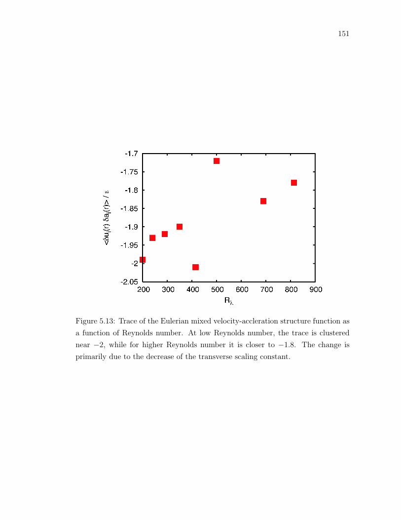
151

Figure 5.13: Trace of the Eulerian mixed velocity-accleration structure function as

a function of Reynolds number. At low Reynolds number, the trace is clustered

near −2, while for higher Reynolds number it is closer to −1.8. The change is

primarily due to the decrease of the transverse scaling constant.

152

Figure 5.14: The same data from Fig. 5.5 shown with the Batchelor prediction

augmented with the third-order correction (solid line). The new model captures

the trend of the deviation, but is not quantitatively correct. It is therefore likely

that the deviation of the data from Batchelor’s law is due either to the influence

of the large scales or to finite volume effects.

high Reynolds number. The trace of the structure function, shown in Fig. 5.13,

is clustered near −2 for the low Reynolds number data, and is closer to −1.8 for

higher Reynolds numbers. Most of this change is due to the smaller transverse

scaling constant.

We have attempted to use this correction term to account for the deviation

of the data from Batchelor’s prediction shown in Fig. 5.5, as shown in Fig. 5.14.

The new model does capture the trend of the data, but deviates from the original

Batchelor prediction at a later time. It is therefore likely that the deviation is due

either to interaction with the large scales or to finite volume effects rather than to

higher-order corrections to Batchelor’s law.

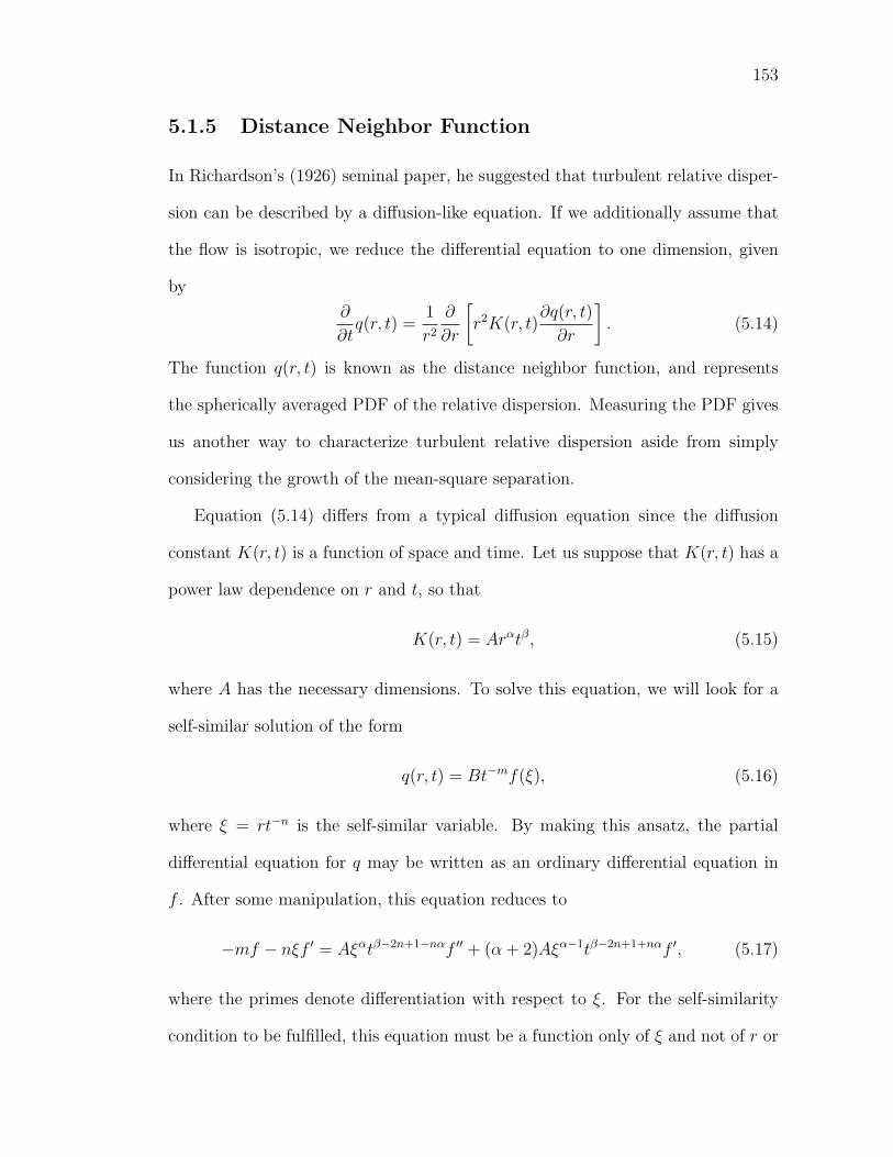
153

5.1.5 Distance Neighbor Function

In Richardson’s (1926) seminal paper, he suggested that turbulent relative disper-

sion can be described by a diffusion-like equation. If we additionally assume that

the flow is isotropic, we reduce the differential equation to one dimension, given

by

∂

∂tq(r, t) =

1

r2

∂

∂r

[r2K(r, t)

∂q(r, t)

∂r

]. (5.14)

The function q(r, t) is known as the distance neighbor function, and represents

the spherically averaged PDF of the relative dispersion. Measuring the PDF gives

us another way to characterize turbulent relative dispersion aside from simply

considering the growth of the mean-square separation.

Equation (5.14) differs from a typical diffusion equation since the diffusion

constant K(r, t) is a function of space and time. Let us suppose that K(r, t) has a

power law dependence on r and t, so that

K(r, t) = Arαtβ, (5.15)

where A has the necessary dimensions. To solve this equation, we will look for a

self-similar solution of the form

q(r, t) = Bt−mf(ξ), (5.16)

where ξ = rt−n is the self-similar variable. By making this ansatz, the partial

differential equation for q may be written as an ordinary differential equation in

f . After some manipulation, this equation reduces to

−mf − nξf ′ = Aξαtβ−2n+1−nαf ′′ + (α + 2)Aξα−1tβ−2n+1+nαf ′, (5.17)

where the primes denote differentiation with respect to ξ. For the self-similarity

condition to be fulfilled, this equation must be a function only of ξ and not of r or

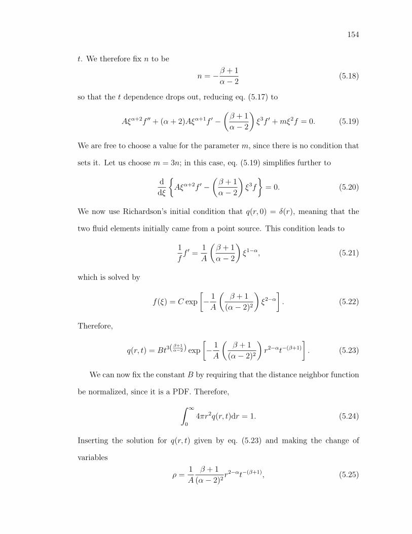
154

t. We therefore fix n to be

n = −β + 1

α− 2(5.18)

so that the t dependence drops out, reducing eq. (5.17) to

Aξα+2f ′′ + (α + 2)Aξα+1f ′ −(β + 1

α− 2

)ξ3f ′ +mξ2f = 0. (5.19)

We are free to choose a value for the parameter m, since there is no condition that

sets it. Let us choose m = 3n; in this case, eq. (5.19) simplifies further to

d

dξ

{Aξα+2f ′ −

(β + 1

α− 2

)ξ3f

}= 0. (5.20)

We now use Richardson’s initial condition that q(r, 0) = δ(r), meaning that the

two fluid elements initially came from a point source. This condition leads to

1

ff ′ =

1

A

(β + 1

α− 2

)ξ1−α, (5.21)

which is solved by

f(ξ) = C exp

[− 1

A

(β + 1

(α− 2)2

)ξ2−α

]. (5.22)

Therefore,

q(r, t) = Bt3(β+1α−2) exp

[− 1

A

(β + 1

(α− 2)2

)r2−αt−(β+1)

]. (5.23)

We can now fix the constant B by requiring that the distance neighbor function

be normalized, since it is a PDF. Therefore,∫ ∞0

4πr2q(r, t)dr = 1. (5.24)

Inserting the solution for q(r, t) given by eq. (5.23) and making the change of

variables

ρ =1

A

β + 1

(α− 2)2r2−αt−(β+1), (5.25)

155

this integral may be written as

4πB

A(2− α)

((α− 2)2

β + 1

) 32−α∫ ∞

0

ρ1+α2−α e−ρdρ = 1. (5.26)

Solving this equation we have

B =

(2− α

4π

)(A

(α− 2)2

β + 1

)− 32−α 1

Γ(

32−α

) . (5.27)

The relative dispersion 〈r2〉 may now be calculated from the distance neighbor

function, since

〈r2〉 =

∫ ∞0

4πr4q(r, t)dr. (5.28)

Making the same change of variables as in eq. (5.25), we find that

〈r2〉 =

(A

(α− 2)2

β + 1

) 22−α

t2(β+12−α) Γ

(5

2−α

)Γ(

32−α

) . (5.29)

In terms of 〈r2〉, we can write the distance neighbor function as

q(r, t) =

(2− α

4π

) [Γ(

52−α

)]3/2[Γ(

32−α

)]5/2 1

〈r2〉3/2exp

−(Γ(

52−α

)Γ(

32−α

) r2

〈r2〉

) 2−α2

. (5.30)

In the inertial range, K41 requires that the constant A can depend only on the

dissipation rate ε. Suppose that A = κεγ, so that

K ∼ εγrαtβ. (5.31)

As K must have units of diffusivity, eq. (5.31) requires that

α = 2(1− γ) (5.32)

and

β = 3γ − 1. (5.33)

156

From eq. (5.29), it is then clear that any choice of α and β consistent both dimen-

sionally and with K41 leads to 〈r2〉 ∼ t3 (Klafter et al., 1987). Comparing with

the Richardson-Obukhov law, the Richardson constant is therefore given by

g =

(4

3κγ

)1/γ Γ(

52γ

)Γ(

32γ

) . (5.34)

Sawford (2001) shows that the Richardson constant is related to the Lagrangian

structure function constant as g = 2C0. This relation further gives

κ =3

4γ

2C0

Γ(

32γ

)Γ(

52γ

)γ . (5.35)

In his initial work, Richardson (1926) suggested that K(r, t) ∼ r4/3 based

on diffusion constants measured in systems ranging from molecular diffusion to

volcanoes and cyclones. With this choice,

qR(r, t) =429

70

√143

2π−3/2(gεt3)−3/2 exp

[−(

1287r2

8gεt3

)1/3], (5.36)

where g is again the Richardson constant. Subsequently, Batchelor (1952) proposed

instead that K(r, t) ∼ t2, which leads to

qB(r, t) =

(2π

3

)−3/2

(gεt3)−3/2 exp

[−3

2

r2

gεt3

]. (5.37)

It is important to recognize that this prediction of Batchelor’s is for the PDF of

the relative dispersion at long times when a Richardson-Obukhov scaling regime

is expected, and is distinct from the t2 Batchelor scaling regime discussed above.

As described above, the solution to the distance neighbor function requires the

initial condition that at t = 0, the two fluid elements were in the same location.

We cannot replicate this condition in the laboratory. By subtracting off the initial

separation of the fluid element pair componentwise, however, we can approximate

157

Figure 5.15: Plots of the distance neighbor function for different initial separations

at Rλ = 815. The red line is Richardson’s predicted PDF, while the green line is

Batchelor’s. The symbols show experimental measurements. Each plot shows a

different initial separation. For each initial separation, PDFs from twenty times

are shown ranging from τη to 20τη. At Rλ = 815, 1 mm ∼ 43η.

158

this condition. We note, however, that not all fluid element pairs separate; some

pairs will first move closer together before later spreading apart. This approach of

subtracting the initial separation from each subsequent pair separation and then

taking the length of this vector will treat both separating and approaching fluid

element pairs in the same fashion.

Our measurements of the distance neighbor function, defined as above, are

shown in Fig. 5.15 for six different initial separations at Rλ = 815. For each

separation, q(r, t) is shown for twenty different times ranging from τη to 20τη. We

find that for small initial separations, the measured distance neighbor function

agrees well with Richardson’s predicted form, while for large initial separations,

the data agree well with Batchelor’s form. For intermediate initial separations,

there is a transition region between the Richardson PDF and the Batchelor PDF.

We see the same qualitative trend in lower Reynolds number data. The dis-

tance neighbor function is shown in Fig. 5.16 for Rλ = 200. Again, as the initial

separation increases, the data make a transition from Richardson’s PDF to Batch-

elor’s.

If we calculate the distance neighbor function without first subtracting the ini-

tial separation, different behavior is seen, as shown in Fig. 5.17. For short times,

the distance neighbor function is strongly peaked around the RMS separation. In

the ideal case where the initial separation r0 is exact and not binned, the distance

neighbor function at t = 0 would be a delta function at the RMS separation. As

time increases, the distance neighbor function spreads out, appearing to approach

the Batchelor prediction regardless of the initial separation. It remains unclear

whether this approach is more justified for calculating the distance neighbor func-

tion or whether we should subtract the initial separation, as shown above, when

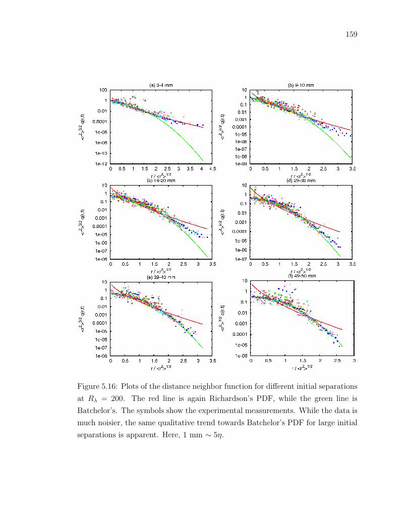
159

Figure 5.16: Plots of the distance neighbor function for different initial separations

at Rλ = 200. The red line is again Richardson’s PDF, while the green line is

Batchelor’s. The symbols show the experimental measurements. While the data is

much noisier, the same qualitative trend towards Batchelor’s PDF for large initial

separations is apparent. Here, 1 mm ∼ 5η.

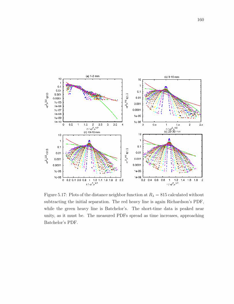
160

Figure 5.17: Plots of the distance neighbor function at Rλ = 815 calculated without

subtracting the initial separation. The red heavy line is again Richardson’s PDF,

while the green heavy line is Batchelor’s. The short-time data is peaked near

unity, as it must be. The measured PDFs spread as time increases, approaching

Batchelor’s PDF.

161

faced with a realistic, physical situation where the fluid elements are not dispersing

from a point source.

5.1.6 Fixed Scale Statistics

In our experiments at Reynolds numbers up to Rλ = 815 we have not observed

the Richardson-Obukhov law in its original form; instead, we observed a regime

consistent with Batchelor’s predictions through most of our inertial range. As we

have shown above, this behavior suggests that a much higher Reynolds number is

required before the Richardson-Obukhov regime can be unambiguously observed.

Because of the appeal of the Richardson-Obukhov prediction, however, researchers

have introduced new statistics in the hope that behavior consistent with it can be

found at the moderate Reynolds numbers reached in experiments and simulations.

We have discussed one such quantity above when we considered 〈r(t)2/3〉 instead

of 〈[ri(t) − r0i]2〉. Instead of studying different averages of the relative particle

separation as a function of time, however, one can also study averages of the time

it takes for the relative separation to grow to a particular threshold. Such averages

of time rather than of space are known as fixed scale statistics since the averaging

is performed over an ensemble at a fixed spatial scale rather than at a fixed tem-

poral scale as in the traditional Richardson-Obukhov or Batchelor description of

turbulent relative dispersion (Boffetta and Celani, 2000). Dimensionally, a scaling

law such as

〈t〉 = Gε−1r2/3 (5.38)

is equivalent to the Richardson-Obukhov law.

A particular type of fixed scale statistics that has become well-known is the

so-called exit time or doubling time statistics introduced by Artale et al. (1997).

162

An exit time analysis defines a set of thresholds rn for every particle pair such

that rn = ρnr0, where ρ is a scale factor. The exit time tρ(rn) is then defined

to be the time it takes for the particle pair to grow from rn to rn+1. For ρ = 2,

t2(rn) is the time it takes for the pair separation to double in size. Exit time

statistics have recently been touted as a powerful alternative to the traditional

analysis of turbulent relative dispersion that should show “true” inertial range

scaling behavior even at moderate Reynolds numbers (Artale et al., 1997; Boffetta

and Celani, 2000; Boffetta and Sokolov, 2002a; Biferale et al., 2005a).

Dimensionally, the ensemble average of the exit times should scale as 〈tρ(rn)〉 ∼

r2/3n . Without some assumptions, however, the exit time analysis cannot be directly

compared with more traditional analyses. In particular, a measurement of the

scaling of the exit times cannot give the value of the Richardson constant g without

assumptions. By assuming the Richardson form for the distance neighbor function,

Boffetta and Sokolov (2002a) have found that

〈tρ(rn)〉 =

(143

81(gε)−1

)1/3ρ2/3 − 1

ρ2/3r2/3n , (5.39)

which in turn gives

g =143

81

(ρ2/3 − 1

)3

ρ2

r2n

ε〈tρ(rn)〉3. (5.40)

Our measurement of the average exit times at Rλ = 815 with ρ = 1.05 is

shown in Fig. 5.18. There is no collapse for data with different initial separations,

though at larger scales the data may be approaching an r2/3n power law as predicted

by Boffetta and Sokolov (2002a). In Fig. 5.19, we show a modified version of

the exit time statistics where we have subtracted the initial pair separation r0

componentwise. With the initial separation subtracted, our results appear more

similar the simulations of Biferale et al. (2005a). Though Biferale et al. (2005a)

163

Figure 5.18: Average exit times at Rλ = 815. The solid line is an r2/3n power law

for reference. From left to right, the symbols correspond to 1 mm wide bins of

initial separations ranging from 1–2 mm to 19–20 mm.

Figure 5.19: Average exit times with the initial separation subtracted at Rλ = 815.

The solid line is again an r2/3n power law for reference. The symbols are the same

as those shown in Fig. 5.18.

164

Figure 5.20: The Richardson constant computed from the exit times with the initial

separation subtracted at Rλ = 815. If the exit time statistics were truly universal

and independent of initial separation, the data plotted in this way should show a

plateau with the same value for each initial separation. This does not appear to

be the case.

did not subtract the initial pair separation, they considered only initial separations

of less than 20η. With r0 that small, initial separation effects may be negligible.

We, however, do not have enough data at initial separations of that scale with

which to test this hypothesis.

As shown above, eq. (5.40) can be used to extract the Richardson constant

from exit time statistics, subject to several assumptions. We show this mapping in

Fig. 5.20 for the exit time statistics with the initial separation subtracted. Biferale

et al. (2005a) claim that this type of plot shows a plateau with with g ≈ 0.5,

irrespective of the initial separation. We, however, see different behavior. While

the data does flatten, there is no universal value observed. In addition, the pu-

tative Richardson constant is two orders of magnitude smaller than that reported

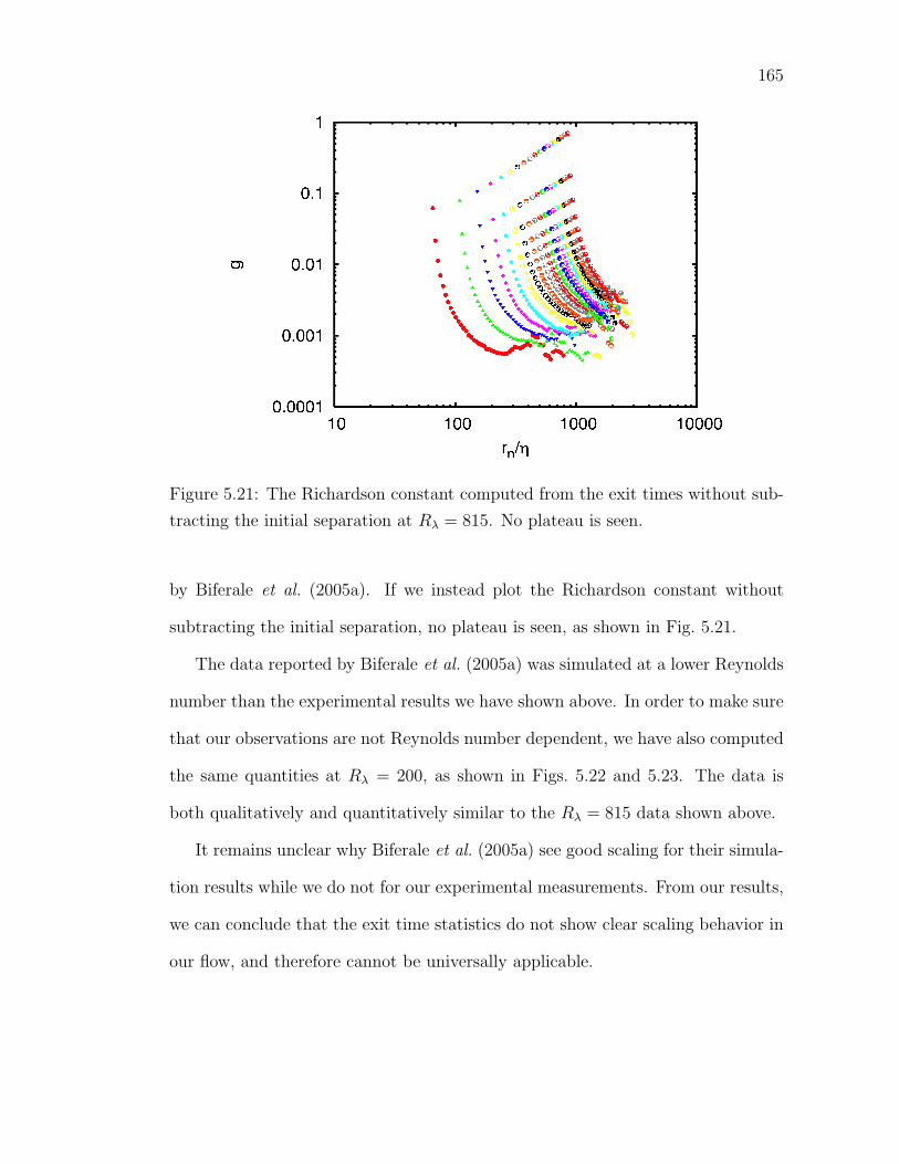
165

Figure 5.21: The Richardson constant computed from the exit times without sub-

tracting the initial separation at Rλ = 815. No plateau is seen.

by Biferale et al. (2005a). If we instead plot the Richardson constant without

subtracting the initial separation, no plateau is seen, as shown in Fig. 5.21.

The data reported by Biferale et al. (2005a) was simulated at a lower Reynolds

number than the experimental results we have shown above. In order to make sure

that our observations are not Reynolds number dependent, we have also computed

the same quantities at Rλ = 200, as shown in Figs. 5.22 and 5.23. The data is

both qualitatively and quantitatively similar to the Rλ = 815 data shown above.

It remains unclear why Biferale et al. (2005a) see good scaling for their simula-

tion results while we do not for our experimental measurements. From our results,

we can conclude that the exit time statistics do not show clear scaling behavior in

our flow, and therefore cannot be universally applicable.

166

Figure 5.22: Average exit times at Rλ = 200. The solid line is an r2/3n power law

for reference. From left to right, the symbols again correspond to 1 mm wide bins

of initial separations ranging from 1–2 mm to 19–20 mm. In the upper plot, we

have not subtracted the initial separations, while in the lower plot we have.

167

Figure 5.23: The Richardson constant computed from the exit times at Rλ = 200.

Behavior similar to that of the Rλ = 815 case is observed.

5.2 Coarse-Grained Models

The Navier-Stokes equations are too complex to solve for realistic boundary con-

ditions. In many situations of practical interest, such as solving for the flow field

around a vehicle or in a turboengine, however, the boundary conditions are incred-

ibly complex. Researchers are therefore turning increasingly to computer simula-

tions to solve these difficult problems. Direct numerical simulation (DNS), where

the Navier-Stokes equations are solved directly, is the most accurate simulation

method known today. Due to limited computer power, however, DNS can only

be used to simulate a relatively small range of scales, and is therefore restricted

to low Reynolds numbers. The problem becomes worse when complex boundary

conditions are included, and so in such cases DNS is not feasible.

Current commercial software packages generally use somewhat crude RANS-

168

level modeling, and the results of the simulation may be quantitatively poor,

though such simulations can reach higher Reynolds numbers. A third technique,

known as Large Eddy Simulation (LES), however, may be able to combine much

of the accuracy of a DNS with the high Reynolds numbers achievable in RANS

models.

Like in DNS, LES solves the Navier-Stokes equations directly on a grid. The

primary difference between DNS and LES is the grid resolution. A DNS grid

resolves the cascade all the way down to the Kolmogorov scale, while an LES grid

is much more coarse. Because of the coarseness of the grid, an LES uses a subgrid-

scale model for the small scales of turbulence, since these scales are presumed to

be universal for all turbulent flows, regardless of how the turbulence is generated.

The fixed computational resources are then free to be used to solve for the large

scale flow directly, and the small scales are given by the model.

The fidelity of an LES to the real situation of interest is determined to a great

degree by the quality of the subgrid-scale model. Many of the commonly used

models have been surveyed by Meneveau and Katz (2000). A new model based

on a coarse-graining of the velocity gradient tensor over a set of four points in the

inertial range has recently been proposed (Chertkov et al., 1999; Pumir et al., 2000,

2001). We have attempted to address the validity of this model experimentally.

5.2.1 Tetrad Dynamics

The central quantity in the model of Chertkov et al. (1999) is a coarse-grained

velocity gradient tensor. Before discussing the model, then, let us consider the

dynamics of the true velocity gradient tensor. Let us define

∂uj∂xi≡ mij (5.41)

169

for simplicity. In the limit of infinite Reynolds number and far away from any

boundaries, the Navier-Stokes equations are well-approximated by the Euler equa-

tions, where the viscosity is set to zero. In that case, the momentum equation

is

∂uj∂t

+ uk∂uj∂xk

= − ∂p

∂xj. (5.42)

Let us now take the gradient of this equation. Since the gradient commutes with

the time differentiation, we have

∂

∂t

∂uj∂xi

+∂

∂xi

(uk∂uj∂xk

)= − ∂2p

∂xi∂xj, (5.43)

which leads to

Dmij

Dt+mikmkj = − ∂2p

∂xi∂xj. (5.44)

Let us now consider the trace of this expression. Due to incompressibility,

Tr m ≡ mii = 0, and so

Tr m2 = −∇2p. (5.45)

We can therefore model the pressure Hessian as

− ∂2p

∂xi∂xj= aij Tr m2 + zij (5.46)

as long as

Tr a = 1 (5.47)

and

Tr z = 0. (5.48)

We identify aij Tr m2 with the local effect of the pressure of the fluid element on

itself and zij with the nonlocal contribution of the pressure due to the rest of the

170

fluid (Vieillefosse, 1984; Cantwell, 1992; Chertkov et al., 1999). We can therefore

write the equation of motion of the velocity gradient as

Dmij

Dt+mikmkj − aij Tr m2 = zij. (5.49)

If we set aij ≡ δij and zij ≡ 0, we recover the “restricted Euler dynamics” intro-

duced by Vieillefosse (1984) and solved analytically by Cantwell (1992).

In LES, as discussed above, the true velocity gradient tensor cannot be deter-

mined. This is also the case in most experimental situations due the difficulty in

measuring spatial gradients. Chertkov et al. (1999) have therefore introduced a

coarse-graining of the velocity gradient tensor defined to be

Mij ≡∫

Γ

∂uj∂xi

dr, (5.50)

where Γ is a time-dependent volume of fluid with a characteristic length scale R

lying in the inertial range. To simplify matters further, Chertkov et al. (1999)

consider the minimal parameterization of such a volume by four fluid elements,

which we label as x1, x2, x3, and x4. This collection of four points is termed a

“tetrad.” In homogeneous, isotropic turbulence, the motion of the center of mass of

the tetrad is irrelevant, and we define three vectors that parameterize the relative

positions of the four points defining the tetrad:

X1 =1√2

(x2 − x1)

X2 =1√6

[(x3 − x2) + (x3 − x1)] (5.51)

X3 =1√12

[(x4 − x3) + (x4 − x2) + (x4 − x1)]

These three vectors may be interpreted as the columns of a matrix X. In the same

ways, we define V to be the matrix of the relative velocities of the four tetrad

171

points by simply replacing the tetrad point positions in eq. (5.51) by the tetrad

point velocities.

Defining K ≡ X−1, we can write the coarse-grained velocity gradient tensor as

Mij = KikVkj −1

3δij Tr(KV), (5.52)

where the term proportional to the Kronecker delta enforces Tr M = 0, as required

by incompressibility. Chertkov et al. (1999) then proceed to assume that this

coarse-grained tensor evolves according to the same equation of motion as the true

velocity gradient tensor, namely by

DMij

Dt+MikMkj − Aij Tr M2 = Zij, (5.53)

where now

Aij ≡KikKkj

Tr K2. (5.54)

A is a measure of the anisotropy of the tetrad. Chertkov et al. (1999) model Z as

a random variable.

The restricted Euler dynamics lie in the phase space spanned by

Q ≡ −1

2Tr M2 (5.55)

and

R ≡ −1

3Tr M3, (5.56)

two of the invariants implied the Cayley-Hamilton theorem (Vieillefosse, 1984;

Cantwell, 1992). The third invariant of M is (Vieillefosse, 1984)

D = 3[Tr M3

]2 − 1

2

[Tr M2

]3= 27R2 + 4Q3. (5.57)

When D = 0, M has degenerate eigenvalues. For D > 0, the eigenvalues of M are

complex and the flow is dominated by vorticity. When D < 0, the eigenvalues are

real and strain dominates the flow (Cantwell, 1992).

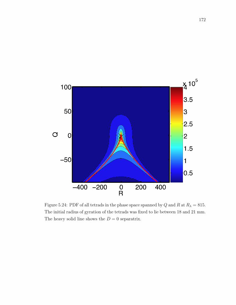
172

Figure 5.24: PDF of all tetrads in the phase space spanned byQ andR atRλ = 815.

The initial radius of gyration of the tetrads was fixed to lie between 18 and 21 mm.

The heavy solid line shows the D = 0 separatrix.

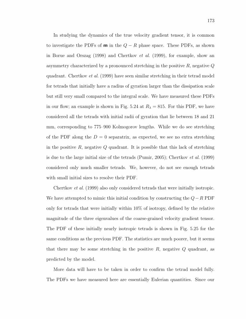
173

In studying the dynamics of the true velocity gradient tensor, it is common

to investigate the PDFs of m in the Q − R phase space. These PDFs, as shown

in Borue and Orszag (1998) and Chertkov et al. (1999), for example, show an

asymmetry characterized by a pronounced stretching in the positive R, negative Q

quadrant. Chertkov et al. (1999) have seen similar stretching in their tetrad model

for tetrads that initially have a radius of gyration larger than the dissipation scale

but still very small compared to the integral scale. We have measured these PDFs

in our flow; an example is shown in Fig. 5.24 at Rλ = 815. For this PDF, we have

considered all the tetrads with initial radii of gyration that lie between 18 and 21

mm, corresponding to 775–900 Kolmogorov lengths. While we do see stretching

of the PDF along the D = 0 separatrix, as expected, we see no extra stretching

in the positive R, negative Q quadrant. It is possible that this lack of stretching

is due to the large initial size of the tetrads (Pumir, 2005); Chertkov et al. (1999)

considered only much smaller tetrads. We, however, do not see enough tetrads

with small initial sizes to resolve their PDF.

Chertkov et al. (1999) also only considered tetrads that were initially isotropic.

We have attempted to mimic this initial condition by constructing the Q−R PDF

only for tetrads that were initially within 10% of isotropy, defined by the relative

magnitude of the three eigenvalues of the coarse-grained velocity gradient tensor.

The PDF of these initially nearly isotropic tetrads is shown in Fig. 5.25 for the

same conditions as the previous PDF. The statistics are much poorer, but it seems

that there may be some stretching in the positive R, negative Q quadrant, as

predicted by the model.

More data will have to be taken in order to confirm the tetrad model fully.

The PDFs we have measured here are essentially Eulerian quantities. Since our

174

Figure 5.25: PDF of initially nearly isotropic tetrads at Rλ = 815. Again, the

initial radius of gyration was fixed to lie between 18 and 21 mm. The heavy solid

line shows the D = 0 separatrix. A small amount of stretching in the positive R,

negative Q quadrant is evident for these tetrads.

175

experiment is inefficient for measuring such quantities, we expect more traditional

Eulerian measurement techniques, particularly multiprobe hot-wire anemometry,

will be more effective for confirming or contradicting the tetrad model.

5.2.2 The Geometry of Turbulence

Pumir et al. (2000) have also investigated the statistical geometry implicit in their

tetrad model. Let us a define a tensor

gij ≡ XikXkj (5.58)

analogous to the inertia tensor of a collection of point masses. The radius of

gyration R of the tetrad, defined as R2 ≡ Tr g, provides a convenient linear measure

of the tetrad size.

Let us consider the eigenvalues of g, which we denote as g1, g2, and g3 where

g1 > g2 > g3. (5.59)

Note that, by definition, g1 + g2 + g3 = R2. We can therefore normalize the

eigenvalues by R2 to force them to lie between zero and one; we denote these

scaled eigenvalues by gi/R2 ≡ Ii. The evolution of the three eigenvalues gives

information on the shape changes of the tetrad. When the three eigenvalues are

equal, the tetrad is a regular tetrahedron. If the eigenvalues are not equal, however,

the tetrad will be anisotropic. If g1 ≈ g2 and g1 � g3, the tetrad will be nearly

planar, while if g1 � g2 and g2 ≈ g3, the tetrad will be needle-like. The evolution

of the tetrad shapes has recently been considered in simulation (Biferale et al.,

2005b), but there have been no experimental studies to date.

We begin by considering the nearly isotropic tetrads introduced above in the

context of the Q−R PDFs for the coarse-grained velocity gradient tensor. The evo-

176

Figure 5.26: The shape evolution of the initially nearly isotropic tetrads at Rλ =

815, as characterized by the eigenvalues of g. As above, the initial radius of

gyration was fixed to lie between 18 and 21 mm.

177

lution of the ensemble averages of the tetrad eigenvalues for these nearly isotropic

tetrads is shown in Fig. 5.26. By construction, the three eigenvalues begin almost

equal to each other. In a very short amount of time, however, the eigenvalues start

to diverge and the shape of the tetrads begins to change. The tetrads flatten from

their initially regular tetrahedral shapes to asymmetric flat, elongated structures

as the largest eigenvalue grows rapidly while the smallest eigenvalue decreases.

Since the three eigenvalues retain different values, however, the tetrads become

effectively two-dimensional as time increases. Unfortunately, it is highly unlikely

that four tracer particles will remain together in our measurement volume for long

times, and so the time range of the eigenvalue evolution we can investigate is very

short; indeed, the sharp drop in g2 in Fig. 5.26 is a manifestation of this problem.

We cannot, therefore, effectively investigate the true scaling behavior of the tetrad

shapes. We also have not considered the removal of the initial size of the tetrads;

in analogy with the two-particle case, the initial size may play an important role in

the tetrad dynamics at short times. It is unclear, however, how to account for the

initial separations of the four particles that make up the the tetrads. Considering

the 〈Ii〉 instead of the 〈gi〉 can account for some of the initial size effect, but other

statistics may be needed as well.

The evolution of the eigenvalues of the full ensemble of tetrads is shown in

Fig. 5.27. The initial ratio of the three eigenvalues effectively shows the steady-

state situation, and compares well with the longer-time behavior we saw for the

eigenvalues in the nearly isotropic case. As seen from the 〈gi〉, the size of all the

tetrads increases with time. When the radius of gyration is scaled out, as shown

in the plot of 〈Ii〉, very little shape change occurs, supporting the interpretation

of the full ensemble of tetrads as representative of the steady-state situation.

178

Figure 5.27: The shape evolution of the full ensemble of tetrads at Rλ = 815, as

characterized by the eigenvalues of g. The initial radius of gyration was fixed to

lie between 18 and 21 mm.

Chapter 6

Conclusions and OutlookIn the preceding chapters, we have presented experimental measurements of the

Lagrangian velocity and position statistics of both single passive tracer particles

and clusters of tracers. We have measured the anomalous scaling of the Lagrangian

structure functions, as well as the scaling constant for the second-order structure

function. We have investigated turbulent relative dispersion in many forms, and

have performed some preliminary experimental tests of the higher-order tetrad

models. We have also made the first experimental measurements of the multi-

fractal dimension spectrum of Lagrangian turbulence. In order to make these

measurements, we have developed a versatile Lagrangian particle tracking system,

and have made a study of tracking algorithms.

And yet, despite the data presented here, experimental studies of Lagrangian

turbulence are in a large part still in their infancy. Only recently have digital cam-

eras become fast enough to track particles accurately at high Reynolds numbers,

and camera speed is still the primary factor that limits the maximum measur-

able Reynolds number. The fastest cameras on the market today also suffer from

small sensor sizes at their maximum imaging speeds. The experimental turbulence

community is therefore eagerly awaiting new advances in imaging technology.

The Lagrangian particle tracking techniques we have described in this thesis are

very powerful for measuring the trajectories of individual tracers and their time

derivatives. But, except for very low Reynolds numbers where the Kolmogorov

scale is relatively large, the measurement of spatial derivatives along particle tra-

jectories is not yet possible (Luthi, 2002). In particular, measurements of the La-

179

180

grangian velocity gradients at high Reynolds number would be of great importance

since the energy dissipation rate ε is so fundamental to the statistical description

of turbulence as we know it. Equivalent information, however, is contained in the

enstrophy dissipation rate. The enstrophy, defined as ω2/2 where ω is the vortic-

ity, is related to the antisymmetric part of the velocity gradient tensor just as the

energy is related to the symmetric part. The primary difference between the two is

experimental: while the local energy dissipation rate cannot be determined with-

out measuring the full velocity gradient tensor, the local vorticity and therefore the

local enstrophy dissipation can in principle be determined by the Vorticity Optical

Probe (VOP) technique developed by Frish and Webb (1981). VOP replaces the

simple transparent tracer particles used in typical LPT experiments with crystals

of lead carbonate encased in spherical polymer shells. Lead carbonate forms a

planar hexagonal crystal that reflects visible light. Every VOP tracer therefore

behaves as a small, Kolmogorov-scale planar mirror. As the tracers feel the local

vorticity field and spin, they will blink on and off. The frequency of this blinking

directly gives the rotation rate and therefore the local flow vorticity without the

need for any numerical differentiation. While there are significant technical chal-

lenges that must be overcome to implement the VOP technique in a high Reynolds

number turbulent flow, VOP has the potential to provide tremendously important

information about Lagrangian turbulence.

Lagrangian particle tracking can also be used to investigate the behavior of

heavy particles in turbulence, that is, particles that are not passive tracers. Many

problems of practical interest are fundamentally problems of the transport of par-

ticulate matter in turbulent flows, including fuel sprays, the formation and growth

of rain droplets in warm clouds (Shaw, 2003), or the transport of pollutants or

181

pathogens in the atmosphere (Brown and Hovmøller, 2002). For all of these ex-

amples, the transported particles have non-neglible inertia compared to the flow,

and their Stokes numbers will be close to or larger than unity. Unlike our pas-

sive tracers, then, these inertial particles will not perfectly follow the flow, and we

therefore expect that their velocities and accelerations will be depressed when com-

pared with a fluid element of the carrier flow. These effects have indeed been seen

in simulation (Bec et al., 2006) and in preliminary experimental work (Ayyalaso-

mayajula et al., 2005), but significant work must still be done to characterize the

Stokes number dependence of turbulence statistics fully.

Irrespective of measurement technique, there are still fundamental issues to be

resolved in the study of turbulence. The most fundamental assumption we have

about turbulence, and the quality of turbulence that makes it such an interesting

problem, is its universality. According to K41, the statistics of turbulence at small

scales are independent of the large-scale flow geometry or forcing. Our results

on the scaling of the Lagrangian structure functions and the dispersion of single

tracer particles call this universality into question, as do previous results from

many other researchers. It is therefore imperative that turbulence statistics be

investigated with the same measurement and analysis techniques in a wide variety

of turbulent flows in order to investigate the extent to which universality holds.

Here, we have used only our von Karman swirling flow, and have found results that,

in some cases, differ from measurements made in wind tunnels, the workhorse of

laboratory flows. Many other types of laboratory flows have also been developed,

including flow between oscillating grids (Mann et al., 1999), in arrays of turbulent

jets (Variano et al., 2004), or in boxes driven by fans or speakers (Hwang and

Eaton, 2004). In addition, natural flows in the atmosphere and oceans provide high

182

Reynolds numbers due to their large scales, though they are less well-controlled.

The questions raised above will soon be under investigation at the Max Planck

Institute for Dynamics and Self-Organization. In addition to the von Karman

water flow used in the experiments reported here, there are plans to build a von

Karman flow with sulfur hexafluoride (SF6), an inert gas heavier than air, as the

working fluid. Construction has already begun on a large-scale wind tunnel using

SF6 pressurized to 15 atmospheres that should be able to reach Reynolds numbers

of order Rλ ∼ 104. In addition, a large “wind box” with dimensions of 5 × 5 × 5

m3 is also planned. The Lagrangian particle tracking system used here will also

be used for each of these flows, in addition to traditional hot wire anemometry

and laser doppler anemometry. There are also plans to develop a working VOP

system for use with these high-Reynolds number flows. The outlook in general for

experimental studies of turbulence is therefore bright, and it is an exciting time to

be working in the field.

REFERENCES

R. J. Adrian. Particle-imaging techniques for experimental fluid mechanics.

Annu. Rev. Fluid Mech., 23:261–304, 1991.

F. Anselmet, Y. Gagne, E. J. Hopfinger, and R. A. Antonia. High-order velocity

structure functions in turbulent shear flow. J. Fluid Mech., 140:63–89, 1984.

V. Artale, G. Boffetta, A. Celani, M. Cencini, and A. Vulpiani. Dispersion of

passive tracers in closed basins: Beyond the diffusion coefficient. Phys. Fluids,

9:3162–3171, 1997.

S. Ayyalasomayajula, A. Gylfason, and Z. Warhaft. Lagrangian measurements of

inertial particles in wind tunnel turbulence. Bull. Am. Phys. Soc., 50:65, 2005.

E. Balkovsky and B. I. Shraiman. Olfactory search at high Reynolds number.

Proc. Natl. Acad. Sci. USA, 99:12589–12593, 2002.

G. K. Batchelor. The theory of axisymmetric turbulence. Proc. R. Soc. Lond. A,

186:480–502, 1946.

G. K. Batchelor. The application of the similarity theory of turbulence to atmo-

spheric diffusion. Q. J. R. Meteorol. Soc., 76:133–146, 1950.

G. K. Batchelor. Diffusion in a field of homogeneous turbulence II. The relative

motion of particles. Proc. Camb. Phil. Soc., 48:345–362, 1952.

G. K. Batchelor. An Introduction to Fluid Dynamics. Cambridge University Press,

Cambridge, England, 1967.

J. Bec, L. Biferale, G. Boffetta, A. Celani, M. Cencini, A. Lanotte, S. Musacchio,

and F. Toschi. Acceleration statistics of heavy particles in turbulence. J. Fluid

Mech., 550:349–358, 2006.

R. Benzi, S. Ciliberto, R. Tripiccione, C. Baudet, F. Massaioli, and S. Succi.

Extended self-similarity in turbulent flows. Phys. Rev. E, 48:R29–R32, 1993.

P. S. Berloff, J. C. McWilliams, and A. Bracco. Material transport in oceanic

gyres. Part I: Phenomenology. J. Phys. Oceanogr., 32:764–796, 2002.

183

184

L. Biferale, G. Boffetta, A. Celani, B. J. Devenish, A. Lanotte, and F. Toschi.

Multifractal statistics of Lagrangian velocity and acceleration in turbulence.

Phys. Rev. Lett., 93:064502, 2004.

L. Biferale, G. Boffetta, A. Celani, B. J. Devenish, A. Lanotte, and F. Toschi.

Lagrangian statistics of particle pairs in homogeneous isotropic turbulence.

Phys. Fluids, 17:115101, 2005a.

L. Biferale, G. Boffetta, A. Celani, B. J. Devenish, A. Lanotte, and F. Toschi.

Multiparticle dispersion in fully developed turbulence. Phys. Fluids, 17:111701,

2005b.

L. Biferale, G. Boffetta, A. Celani, A. Lanotte, and F. Toschi. Particle trapping in

three-dimensional fully developed turbulence. Phys. Fluids, 17:021701, 2005c.

G. Boffetta and A. Celani. Pair dispersion in turbulence. Physica A, 280:1–9,

2000.

G. Boffetta, F. De Lillo, and S. Musacchio. Lagrangian statistics and temporal

intermittency in a shell model of turbulence. Phys. Rev. E, 66:066307, 2002.

G. Boffetta and I. M. Sokolov. Relative dispersion in fully developed turbulence:

the Richardson’s law and intermittency corrections. Phys. Rev. Lett., 88:094501,

2002a.

G. Boffetta and I. M. Sokolov. Statistics of two-particle dispersion in two-

dimensional turbulence. Phys. Fluids, 14:3224–3232, 2002b.

M. S. Borgas. The multifractal Lagrangian nature of turbulence.

Phil. Trans. R. Soc. Lond. A, 342:379–411, 1993.

V. Borue and S. A. Orszag. Local energy flux and subgrid-scale statistics in three-

dimensional turbulence. J. Fluid Mech., 366:1–31, 1998.

F. Bourgeois and J.-C. Lasalle. An extension of the Munkres algorithm for the

assignment problem to rectangular matrices. Commun. ACM, 14:802–804, 1971.

M. Bourgoin, N. T. Ouellette, H. Xu, J. Berg, and E. Bodenschatz. The role of

pair dispersion in turbulent flow. Science, 311:835–838, 2006.

185

J. K. M. Brown and M. S. Hovmøller. Aerial dispersal of pathogens on the global

and continental scales and its impact on plant disease. Science, 297:537–541,

2002.

B. J. Cantwell. Exact solution of a restricted Euler equation for the velocity

gradient tensor. Phys. Fluids A, 4:782–793, 1992.

F. Carosone, A. Cenedese, and G. Querzoli. Recognition of partially overlapped

particle images using the Kohonen neural network. Exp. Fluids, 19:225–232,

1995.

S. Chandrasekhar. The theory of axisymmetric turbulence.

Phil. Trans. R. Soc. Lond. A, 242:557–577, 1950.

K. Chang, H. Xu, N. T. Ouellette, and E. Bodenschatz. Experimental measure-

ments of the Lagrangian Kolmogorov constant. In preparation, 2006.

S. Y. Chen, B. Dhruva, S. Kurien, K. R. Sreenivasan, and M. A. Taylor. Anomalous

scaling of low-order structure functions of turbulent velocity. J. Fluid Mech.,

533:183–192, 2005.

Y. Chen and A. T. Chwang. Particle image velocimetry system with self-organized

feature map algorithm. J. Eng. Mech.—ASCE, 129:1156–1163, 2003.

M. Chertkov, A. Pumir, and B. I. Shraiman. Lagrangian tetrad dynamics and the

phenomenology of turbulence. Phys. Fluids, 11:2394–2410, 1999.

D. Chetverikov and J. Verestoy. Feature point tracking for incomplete trajectories.

Computing, 62:321–338, 1999.

L. Chevillard. Description multifractale unifiee du phenomene d’intermittence en

turbulence Eulerienne et Lagrangienne. PhD thesis, Universite Bordeaux I, 2004.

L. Chevillard, A. Arneodo, B. Castaing, E. Leveque, J.-F. Pinton, and S. G. Roux.

Unified multifractal description of Eulerian and Lagrangian velocity increments

in turbulence. Bull. Am. Phys. Soc., 50:53, 2005.

L. Chevillard, S. G. Roux, E. Leveque, N. Mordant, J.-F. Pinton, and A. Ar-

neodo. Lagrangian velocity statistics in turbulent flows: effects of dissipation.

Phys. Rev. Lett., 91:214502, 2003.

186

A. B. Chhabra, C. Meneveau, R. V. Jensen, and K. R. Sreenivasan. Direct deter-

mination of the f(α) singularity spectrum and its application to fully developed

turbulence. Phys. Rev. A, 40:5284–5294, 1989.

W.-C. Chiu and L. N. Rib. The rate of dissipation of energy and the energy

spectrum in a low-speed turbulent jet. T. Am. Geophys. Union, 37:13–26, 1956.

L. Collins, 2003. Personal communication.

E. A. Cowen and S. G. Monismith. A hybrid digital particle tracking velocimetry

technique. Exp. Fluids, 22:199–211, 1997.

A. M. Crawford. Particle tracking measurements in fully developed turbulence:

water and dilute polymer solutions. PhD thesis, Cornell University, 2004.

D.-H. Doh, D.-H. Kim, S.-H. Choi, S.-D. Hong, T. Saga, and T. Kobayashi. Single-

frame (two-field image) 3-D PTV for high speed flows. Exp. Fluids, 29:S85–S98,

2000.

T. Dracos. Particle tracking in three-dimensional space. In T. Dracos, editor,

Three-Dimensional Velocity and Vorticity Measuring and Image Analysis Tech-

niques, pages 129–152. Kluwer Academic Publishers, Dordrecht, the Nether-

lands, 1996.

S. Edouard, B. Legras, F. Lefevre, and R. Eymard. The effect of small-scale

inhomogeneities on ozone depletion in the arctic. Nature, 384:444–447, 1996.

G. Falkovich, 2005. Personal communication.

R. P. Feynman, R. B. Leighton, and M. L. Sands. The Feynman Lectures on

Physics, volume 1. Addison-Wesley, Reading, MA, 1963.

U. Frisch. Turbulence: The Legacy of A. N. Kolmogorov. Cambridge University

Press, Cambridge, England, 1995.

M. B. Frish and W. W. Webb. Direct measurement of vorticity by optical probe.

J. Fluid Mech., 107:173–200, 1981.

S. Garg and Z. Warhaft. On the small scale structure of simple shear flow.

Phys. Fluids, 10:662–673, 1998.

187

G. Gioia, G. Lacorata, E. P. Marques Filho, A. Mazzino, and U. Rizza. Richard-

son’s law in large-eddy simulations of boundary-layer flows. Boundary-Layer

Meteorol., 113:187–199, 2004.

I. Grant and X. Pan. The use of neural techniques in PIV and PTV.

Meas. Sci. Tech., 8:1399–1405, 1997.

I. Grant, X. Pan, F. Romano, and X. Wang. Neural-network method applied

to the stereo image correspondence problem in three-component particle image

velocimetry. Appl. Optics, 37:3656–3663, 1998.

Y. G. Guezennec, R. S. Brodkey, N. Trigui, and J. C. Kent. Algorithms for fully

automated three-dimensional particle tracking velocimetry. Exp. Fluids, 17:

209–219, 1994.

S. R. Hanna. Lagrangian and Eulerian time-scale relations in the daytime boundary

layer. J. Appl. Meteorol., 20:242–249, 1981.

R. J. Hill. Opportunities for use of exact statistical equations. Accepted for pub-

lication in J. Turbul.; also preprint physics/0512038 at http://www.arxiv.org,

2005.

K. D. Hinsch and H. Hinrichs. Three-dimensional particle velocimetry. In T. Dra-

cos, editor, Three-Dimensional Velocity and Vorticity Measuring and Image

Analysis Techniques, pages 129–152. Kluwer Academic Publishers, Dordrecht,

the Netherlands, 1996.

M. Huber, J. C. McWilliams, and M. Ghil. A climatology of turbulent dispersion

in the troposphere. J. Atmos. Sci., 58:2377–2394, 2001.

W. Hwang and J. K. Eaton. Creating homogeneous and isotropic turbulence with-

out a mean flow. Exp. Fluids, 36:444–454, 2004.

T. Ishihara and Y. Kaneda. Relative diffusion of a pair of fluid particles in the

inertial subrange of turbulence. Phys. Fluids, 14:L69–L72, 2002.

J. B. Jørgensen, J. Mann, S. Ott, H. L. Pecseli, and J. Trulsen. Experimental

studies of occupation and transit times in turbulent flows. Phys. Fluids, 17:

035111, 2005.

188

L. V. King. On the convection of heat from small cylinders in a stream of fluid.

Determination of convective constants of small platinum wires with application

to hot-wire anemometry. Phil. Trans. R. Soc. Lond. A, 214:373–432, 1914.

J. Klafter, A. Blumen, and M. F. Shlesinger. Stochastic pathway to anomalous

diffusion. Phys. Rev. A, 35:3081–3085, 1987.

A. N. Kolmogorov. The local structure of turbulence in incompressible viscous

fluid for very large Reynolds numbers. Dokl. Akad. Nauk SSSR, 30:301–305,

1941a.

A. N. Kolmogorov. Dissipation of energy in the locally isotropic turbulence.

Dokl. Akad. Nauk SSSR, 32:16–18, 1941b.

A. N. Kolmogorov. On the representation of continuous functions of many vari-

ables by superpositions of continuous functions of one variable and addition.

Dokl. Akad. Nauk SSSR, 114:953–956, 1957.

A. N. Kolmogorov. A refinement of previous hypotheses concerning the local struc-

ture of turbulence in a viscous incompressible fluid at high Reynolds number.

J. Fluid Mech., 13:82–85, 1962.

R. H. Kraichnan. Dispersion of particle pairs in homogeneous turbulence.

Phys. Fluids, 9:1937–1943, 1966.

S. Kurien and K. R. Sreenivasan. Dynamical equations for high-order structure

functions, and a comparison of a mean-field theory with experiments in three-

dimensional turbulence. Phys. Rev. E, 64:056302, 2001.

A. La Porta, G. A. Voth, A. M. Crawford, J. Alexander, and E. Bodenschatz.

Fluid particle accelerations in fully developed turbulence. Nature, 409:1017–

1019, 2001.

G. Labonte. A new neural network for particle-tracking velocimetry. Exp. Fluids,

26:340–346, 1999.

G. Labonte. Neural network reconstruction of fluid flows from tracer-particle dis-

placements. Exp. Fluids, 30:399–409, 2001.

R.-C. Lien and E. A. D’Asaro. The Kolmogorov constant for the Lagrangian

velocity spectrum and structure function. Phys. Fluids, 14:4456–4459, 2002.

189

R.-C. Lien, E. A. D’Asaro, and G. T. Dairiki. Lagrangian frequency spectra of ver-

tical velocity and vorticity in high-Reynolds-number oceanic turbulence. J. Fluid

Mech., 362:177–198, 1998.

B. Luthi. Some aspects of strain, vorticity and material element dynamics as

measured with 3D particle tracking velocimetry in a turbulent flow. PhD thesis,

Swiss Federal Insitute of Technology, Zurich, 2002.

H.-G. Maas. Contributions of digital photogrammetry to 3-D PTV. In T. Dracos,

editor, Three-Dimensional Velocity and Vorticity Measuring and Image Anal-

ysis Techniques, pages 191–207. Kluwer Academic Publishers, Dordrecht, the

Netherlands, 1996.

H.-G. Maas, A. Gruen, and D. Papantoniou. Particle tracking velocimetry in

three-dimensional flows—Part 1. Photogrammetric determination of particle co-

ordinates. Exp. Fluids, 15:133–146, 1993.

N. A. Malik, T. Dracos, and D. A. Papantoniou. Particle tracking velocimetry

in three-dimensional flows—Part 2. Particle tracking. Exp. Fluids, 15:279–294,

1993.

B. B. Mandelbrot. Intermittent turbulence in self-similar cascades: divergence of

high moments and dimension of the carrier. J. Fluid Mech., 62:331–358, 1974.

J. Mann, S. Ott, and J. S. Andersen. Experimental study of relative, turbulent

diffusion. Technical Report Risø-R-1036(EN), Risø National Laboratory, 1999.

I. M. Mazzitelli and D. Lohse. Lagrangian statistics for fluid particles and bubbles

in turbulence. New J. Phys., 6:203, 2004.

C. Meneveau and J. Katz. Scale-invariance and turbulence models for large-eddy

simulation. Annu. Rev. Fluid Mech., 32:1–32, 2000.

C. Meneveau and K. R. Sreenivasan. The multifractal spectrum of the dissipation

field in turbulent flows. Nucl. Phys. B Proc. Suppl., 2:49–76, 1987.

T. M. Mitchell. Machine Learning. McGraw-Hill, Boston, MA, 1997.

A. S. Monin and A. M. Yaglom. Statistical Fluid Mechanics, volume 2. MIT Press,

Cambridge, MA, 1975.

190

P. Moore and J. Crimaldi. Odor landscapes and animal behavior: tracking odor

plumes in different physical worlds. J. Marine Syst., 49:55–64, 2004.

N. Mordant. Mesure lagrangienne en turbulence: mise en œuvre et analyse. PhD

thesis, Ecole Normale Superieure de Lyon, 2001.

N. Mordant, A. M. Crawford, and E. Bodenschatz. Experimental Lagrangian

acceleration probability density function measurement. Physica D, 193:245–

251, 2004a.

N. Mordant, E. Leveque, and J.-F. Pinton. Experimental and numerical study of

the Lagrangian dynamics of high Reynolds turbulence. New J. Phys., 6:116,

2004b.

N. Mordant, P. Metz, O. Michel, and J.-F. Pinton. Measurement of Lagrangian

velocity in fully developed turbulence. Phys. Rev. Lett., 87:214501, 2001.

J. F. Muzy, E. Bacry, and A. Arneodo. Multifractal formalism for fractal signals:

the structure-function approach versus the wavelet-transform modulus-maxima

method. Phys. Rev. E, 47:875–884, 1993.

M. Nelkin and R. M. Kerr. Decay of scalar variance in terms of a modified Richard-

son law for pair dispersion. Phys. Fluids, 24:1754–1756, 1981.

F. Nicolleau and G. Yu. Two-particle diffusion and locality assumption. Phys. Flu-

ids, 16:2309–2321, 2004.

A. M. Obukhov. Spectral energy distribution in turbulent flow. Izv. Akad. Nauk

SSSR, 5:453–566, 1941.

K. Ohmi and H.-Y. Li. Particle-tracking velocimetry with new algorithms.

Meas. Sci. Tech., 11:603–616, 2000.

S. Ott and J. Mann. An experimental investigation of the relative diffusion of

particle pairs in three-dimensional turbulent flow. J. Fluid Mech., 422:207–223,

2000.

N. T. Ouellette, H. Xu, and E. Bodenschatz. A quantitative study of three-

dimensional Lagrangian particle tracking algorithms. Exp. Fluids, 40:301–313,

2006a.

191

N. T. Ouellette, H. Xu, M. Bourgoin, and E. Bodenschatz. An experimental study

of turbulent relative dispersion models. In preparation, 2006b.

N. T. Ouellette, H. Xu, M. Bourgoin, and E. Bodenschatz. Small-scale anisotropy

in Lagrangian turbulence. In review, 2006c.

M. Ould-Rouiss. The axisymmetric equivalent of Kolmogorov’s equation.

Eur. Phys. J. B, 23:107–120, 2001.

G. Parisi and U. Frisch. On the singularity structure of fully developed turbu-

lence. In M. Ghil, R. Benzi, and G. Parisi, editors, Turbulence and Predictability

in Geophysical Fluid Dynamics and Climate Dynamics, pages 84–88. North-

Holland, Amsterdam, the Netherlands, 1985.

M. Pashtrapanshka and W. van de Water. The dispersion of microscopic molecular

clouds in turbulence. Bull. Am. Phys. Soc., 50:153–154, 2005.

S. B. Pope. Turbulent Flows. Cambridge University Press, Cambridge, England,

2000.

C. Poulain, N. Mazellier, P. Gervais, Y. Gagne, and C. Baudet. Spectral vorticity

and Lagrangian velocity measurements in turbulent jets. Flow Turbul. Combust.,

72:245–271, 2004.

W. H. Press, S. A. Teukolsky, W. T. Vetterling, and B. P. Flannery. Numerical

Recipes in C: The Art of Scientific Computing. Cambridge University Press,

Cambridge, England, 1992.

A. Pumir. Turbulence in homogeneous shear flows. Phys. Fluids, 8:3112–3127,

1996.

A. Pumir, 2005. Personal communication.

A. Pumir and B. I. Shraiman. Persistent small scale anisotropy in homogeneous

shear flows. Phys. Rev. Lett., 75:3114–3117, 1995.

A. Pumir, B. I. Shraiman, and M. Chertkov. Geometry of Lagrangian dispersion

in turbulence. Phys. Rev. Lett., 85:5324–5327, 2000.

A. Pumir, B. I. Shraiman, and M. Chertkov. The Lagrangian view of energy

transfer in turbulent flow. Europhys. Lett., 56:379–385, 2001.

192

L. F. Richardson. Weather Prediction by Numerical Process. Cambridge University

Press, Cambridge, England, 1922.

L. F. Richardson. Atmospheric diffusion shown on a distance-neighbour graph.

Proc. R. Soc. Lond. A, 110:709–737, 1926.

H. C. Rodean. The universal constant for the Lagrangian structure function.

Phys. Fluids A, 3:1479–1480, 1991.

D. F. Rogers and J. A. Adams. Mathematical Elements for Computer Graphics.

McGraw-Hill, Boston, 1990.

B. L. Sawford. Reynolds number effects in Lagrangian stochastic models of turbu-

lent dispersion. Phys. Fluids A, 3:1577–1586, 1991.

B. L. Sawford. Turbulent relative dispersion. Annu. Rev. Fluid Mech., 33:289–317,

2001.

I. K. Sethi and R. Jain. Finding trajectories of feature points in a monocular image

sequence. IEEE T. Pattern Anal., 9:56–73, 1987.

R. A. Shaw. Particle-turbulence interactions in atmospheric clouds.

Annu. Rev. Fluid Mech., 35:183–227, 2003.

Z.-S. She and E. Leveque. Universal scaling laws in fully developed turbulence.

Phys. Rev. Lett., 72:336–339, 1994.

X. Shen and Z. Warhaft. The anisotropy of the small scale structure in high

Reynolds number (rλ ∼ 1000) turbulent shear flow. Phys. Fluids, 12:2976–2989,

2000.

B. I. Shraiman and E. D. Siggia. Scalar turbulence. Nature, 405:639–646, 2000.

D. A. Siegel, B. P. Kinlan, B. Gaylord, and S. D. Gaines. Lagrangian descriptions

of marine larval dispersion. Mar. Ecol. Prog. Ser., 260:83–96, 2003.

K. R. Sreenivasan. On the universality of the Kolmogorov constant. Phys. Fluids,

7:2778–2784, 1995.

K. R. Sreenivasan. Anomalous scaling in 3D turbulence. LANL Center for Non-

linear Studies Workshop on Multi-Scale Interactions in Turbulent Flows, 2005.

193

K. R. Sreenivasan and A. Bershadskii. Logarithmic scaling in the near-dissipation

range of turbulence. Pramana–J. Phys., 64:315–321, 2005.

K. R. Sreenivasan, S. I. Vainshtein, R. Bhiladvala, I. San Gil, S. Chen, and N. Cao.

Asymmetry of velocity increments in fully developed turbulence and the scaling

of low-order moments. Phys. Rev. Lett., 77:1488–1491, 1996.

G. I. Taylor. Diffusion by continuous movements. Proc. Lond. Math. Soc., 20:

196–212, 1922.

D. J. Thomson and B. J. Devenish. Particle pair separation in kinematic simula-

tions. J. Fluid Mech., 526:277–302, 2005.

R. Y. Tsai. A versatile camera calibration technique for high-accuracy 3D

machine vision metrology using off-the-shelf TV cameras and lenses. IEEE

T. Robotic. Autom., RA-3:323–344, 1987.

E. A. Variano, E. Bodenschatz, and E. A. Cowen. A random synthetic jet array

driven turbulence tank. Exp. Fluids, 37:613–615, 2004.

C. J. Veenman, M. J. T. Reinders, and E. Backer. Resolving motion correspondence

for densely moving points. IEEE T. Pattern Anal., 23:54–72, 2001.

C. J. Veenman, M. J. T. Reinders, and E. Backer. Establishing motion correspon-

dence using extended temporal scope. Artif. Intell., 145:227–243, 2003.

P. Vieillefosse. Internal motion of a small element of fluid in an inviscid flow.

Physica A, 125:150–162, 1984.

T. von Karman and L. Howarth. On the statistical theory of isotropic turbulence.

Proc. R. Soc. Lond. A, 164:192–215, 1938.

G. A. Voth. Lagrangian acceleration measurements in turbulence at large Reynolds

numbers. PhD thesis, Cornell University, 2000.

G. A. Voth, A. La Porta, A. M. Crawford, J. Alexander, and E. Bodenschatz.

Measurement of particle accelerations in fully developed turbulence. J. Fluid

Mech., 469:121–160, 2002.

194

G. A. Voth, A. La Porta, A. M. Crawford, C. Ward, E. Bodenschatz, and J. Alexan-

der. A silicon strip detector system for high resolution particle tracking in tur-

bulence. Rev. Sci. Instr., 12:4348–4353, 2001.

Z. Warhaft. Turbulence in nature and in the laboratory.

Proc. Natl. Acad. Sci. USA, 99:2481–2486, 2002.

K. A. Weinman and A. Y. Klimenko. Estimation of the Kolmogorov constant c0 by

direct numerical simulation of a continuous scalar. Phys. Fluids, 12:3205–3220,

2000.

J. Westerweel. Digital particle image velocimetry—theory and applications. PhD

thesis, Delft University, 1993.

M. C. Wolf, R. Voigt, and P. A. Moore. Spatial arrangement of odor sources

modifies the temporal aspects of crayfish search strategies. J. Chem. Ecol., 30:

501–517, 2004.

H. Xu, M. Bourgoin, N. T. Ouellette, and E. Bodenschatz. High order Lagrangian

velocity statistics in turbulence. Phys. Rev. Lett., 96:024503, 2006a.

H. Xu, N. T. Ouellette, and E. Bodenschatz. The multifractal dimension of La-

grangian turbulence. Accepted for publication in Phys. Rev. Lett., 2006b.

P. K. Yeung. Direct numerical simulation of two-particle relative diffusion in

isotropic turbulence. Phys. Fluids, 6:3416–3428, 1994.

P. K. Yeung. Lagrangian characteristics of turbulence and scalar transport in direct

numerical simulations. J. Fluid Mech., 427:241–247, 2001.

P. K. Yeung. Lagrangian investigations of turbulence. Annu. Rev. Fluid Mech.,

34:115–142, 2002.

P. K. Yeung and M. S. Borgas. Relative dispersion in isotropic turbulence. Part 1.

Direct numerical simulations and Reynolds-number dependence. J. Fluid Mech.,

503:93–124, 2004.

P. K. Yeung, D. A. Donzis, E. A. Kurth, and S. B. Pope. Reynolds number

dependence of Lagrangian velocity, acceleration, and dissipation statistics in

large numerical simulations of isotropic turbulence. Bull. Am. Phys. Soc., 50:

76, 2005.

195

P. J. Zandbergen and D. Dijkstra. Von Karman swirling flows. Annu. Rev. Fluid

Mech., 19:465–491, 1987.