problem 2-1 - engineering.purdue.edu · me 579 fourier methods in digital signal processing...

ME 579 Fourier Methods in Digital Signal ProcessingHomework Set 2

Homework Due in Class on Friday, February 1st, 2019 - Period 11

Problem 2-1

A signal is comprised of 3 sine waves with amplitudes 6, 4 and 3 with frequencies 20, 30 and 50 Hz,respectively. This signal is sampled at 64 samples per second 64 samples are used to calculate the Ckusing the 1

NDFT(xn,N), where DFT(xn,N) is the N -point Discrete Fourier Transform of the N samplesof the signal: xn, n = 0, 1, 2, ...N − 1. Here N=64.

(a) Write a program to simulate the signal generating the samples, and then use the formula describedabove to calculate the Ck. Plot the one-sided power spectrum.

(b) Sketch the one-sided power spectrum that you would expect for x(t) and compare that spectrumwith your program output.

(c) What is the relationship between the Fourier Series coefficient estimates using your program, Ck,and the true Fourier Series coefficients, Ck? Use this to explain the causes of the differences youidentified in part (b).

(d) Modify your program in part (a) for a signal that is comprised of 3 sine waves with amplitudes 6,4 and 3 with frequencies 10, 30 and 50 rads/sec (rather than Hz), respectively, and sampled at 64samples per second. What should the Ck be in this case, and how does your computer generatedpower spectrum (based on Ck) compare to the true power spectrum? What is the problem withthe computer generated spectrum generated from the 64 data points.

SOLUTION

(a) In this question, I used the MATLAB function fft to do the DFT, but it is OK if you wroteyour own program to do that. In the listing below, I have the calculations for (a), (b), and (d).Instead of plotting the true power spectra by hand I plotted them in MATLAB, but plotting byhand is acceptable, too. Note that I have not included the code for myplot.m and vividoc.m. SeeHomework 1 solution for that code.

%hw2q1.m%%-------Part (a) ---------%N=64;fs=64;Dur=N/fs;

1

Spring 2019 ME579 Homework Set 2 2

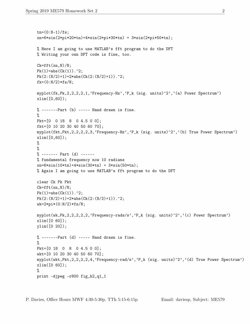
tn=(0:N-1)/fs;xn=6*sin(2*pi*20*tn)+4*sin(2*pi*30*tn) + 3*sin(2*pi*50*tn);

% Here I am going to use MATLAB’s fft program to do the DFT% Writing your own DFT code is fine, too.

Ck=fft(xn,N)/N;Pk(1)=abs(Ck(1)).^2;Pk(2:(N/2)+1)=2*abs(Ck(2:(N/2)+1)).^2;fk=(0:N/2)*fs/N;

myplot(fk,Pk,2,2,2,2,1,’Frequency-Hz’,’P_k (sig. units)^2’,’(a) Power Spectrum’)xlim([0,60]);

% -------Part (b) ----- Hand drawn is fine.%Pkt=[0 0 18 8 0 4.5 0 0];fkt=[0 10 20 30 40 50 60 70];myplot(fkt,Pkt,2,2,2,2,3,’Frequency-Hz’,’P_k (sig. units)^2’,’(b) True Power Spectrum’)xlim([0,60]);%%% ------- Part (d) ------% fundamental frequency now 10 radiansxn=6*sin(10*tn)+4*sin(30*tn) + 3*sin(50*tn);% Again I am going to use MATLAB’s fft program to do the DFT

clear Ck Pk PktCk=fft(xn,N)/N;Pk(1)=abs(Ck(1)).^2;Pk(2:(N/2)+1)=2*abs(Ck(2:(N/2)+1)).^2;wk=2*pi*(0:N/2)*fs/N;

myplot(wk,Pk,2,2,2,2,2,’Frequency-rads/s’,’P_k (sig. units)^2’,’(c) Power Spectrum’)xlim([0 60]);ylim([0 20]);

% -------Part (d) ----- Hand drawn is fine.%Pkt=[0 18 0 8 0 4.5 0 0];wkt=[0 10 20 30 40 50 60 70];myplot(wkt,Pkt,2,2,2,2,4,’Frequency-rad/s’,’P_k (sig. units)^2’,’(d) True Power Spectrum’)xlim([0 60]);%print -djpeg -r800 fig_h2_q1_1

P. Davies, Office Hours MWF 4:30-5:30p, TTh 5:15-6:15p Email: daviesp, Subject: ME579


Figure 2.1.1: (a) and (c) are one-sided power spectra calculated using the scaled Discrete FourierTransform. (b) and (d) are the true power spectra given the components in the signals.

(b) See Figure 2.1.1 (b), and part (c) for the discussion on the calculated versus the actual Fourierseries coefficients.

(c) Because 1 second of data (10 periods of the signal) was used in the calculation, the frequencycomponents are every 1 Hz (inverse of time span of data) in the calculated power spectrum,instead of the every 10 Hz in the true spectrum. With data sampled at 64 samples per second,0.1 seconds are spanned by 6.4 data points, so we cannot get a 10 Hz resolution spectrum whenwe are using the DFT approach. We could have used half a second (32 samples) and then thefrequency spacing would have been 2 Hz.

Because the 50 Hz component is greater than half the sampling rate, it will be aliased when



sampled at 64 samples per second and will appear at 0.5fs− (50− 0.5fs) = fs− 50 = 64− 50 =14Hz.

(d) In this case we cannot synchronize to get a whole number of samples to represent a whole numberof periods. Our sample rate is 64 samples per second and we have 1 second of data (64 points).The frequencies in Hz are irrational numbers: 5

π ,15π ,

25π and the period is 0.2π seconds. So we

cannot take a whole number of samples and span a whole number of periods, i.e., there is nointeger q such that k

q0.2π can equal fs = 64.

If you use 164DFT [xn, 64] to try to estimate the Fourier series coefficients, you will actually be

analyzing a signal of period 64∆=1 second, which will have discontinuities at integer multiplies of1 second. Shown in Figure 2.1.1 (c) are the results of doing this calculation and in Figure 2.1.1 (d)is the true power spectrum. So that you can compare the two spectra easily, the frequencies arerad/s for these two plots. You can see that none of the frequency components in the calculatespower spectrum are at 10, 30 or 50 rad/s and none of them are zero. The resolution of thecalculated spectrum is 2 π rad/s.

There is no aliasing here because the highest frequency in the signal is 50 rad/s and that is lowerthan half the sampling rate: πfs = 64π rad/s.



Problem 2-2

Download the .mat signal posted with this homework and use the load to bring the data into theMATLAB workspace. This time history has been sampled so that N∆ = qTp where N and q areintegers and ∆ is the sampling interval in seconds. The sample rate fs is given in the .mat file.

(a) Determine the smallest number of points, N , that span a whole number of periods. Extract thosefrom the time history, and repeat them an additional two times. Compare the result to the first3N points in the original time history. They should be exactly the same if you got N correct.Show this comparison, and describe your strategy for finding N .

(b) Use the N data points to calculate the Ck and plot the amplitude and phase spectra.

(c) What is the fundamental frequency? What sine and cosine components are in the signal? Generatethis signal and compare to the signal you loaded into the workspace.

SOLUTION

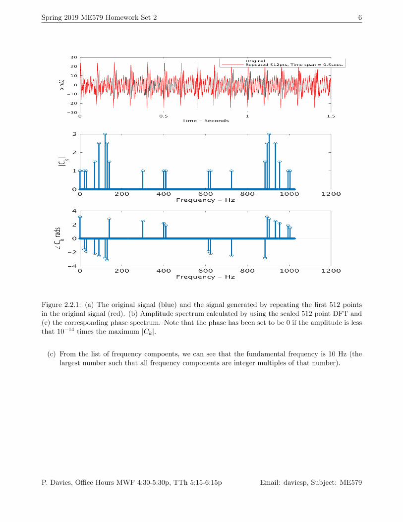
(a) Plotting the signal there appears to be repetition of features every 0.1 seconds, but at this samplerate 0.1 fs is not a whole number (102.4 points). We would need to take 5 periods to get a wholenumber of periods represented by 512∆ seconds. The spectral components in the calculatedspectrum will be spaced every 1

0.5 = 2 Hz. In Figure 2.2.2 (a) is the original signal (blue) and thesignal made by repeating the first 512 points in the signal (red). The red plot lies on top of theblue top.

(b) The calculated amplitude and phase spectra are shown in Figure 2.2.2 (b) and (c), respectively.Code was written to set phase values of very small components to zero and to identify frequenciesand values of all other components. There is a non-zero C0 term and 10 other frequency components.The following is in the diary file after running the program:

Freq (Hz) CCk = 0.5Akk - j 0.5Bkk0 -1.00000 +j 0.00000

20 -0.00000 +j -1.0000030 -0.30902 +j -0.9510670 -0.88168 +j -1.2135390 -2.02254 +j -1.46946

120 -2.85317 +j -0.92705130 -2.50000 +j -0.00000140 -1.42658 +j 0.46353300 -0.80902 +j 0.58779400 -0.58779 +j 0.80902410 -0.30902 +j 0.95106



Figure 2.2.1: (a) The original signal (blue) and the signal generated by repeating the first 512 pointsin the original signal (red). (b) Amplitude spectrum calculated by using the scaled 512 point DFT and(c) the corresponding phase spectrum. Note that the phase has been set to be 0 if the amplitude is lessthat 10−14 times the maximum |Ck|.

(c) From the list of frequency compoents, we can see that the fundamental frequency is 10 Hz (thelargest number such that all frequency components are integer multiples of that number).



Figure 2.2.2: (a) The original signal (blue) and the signal generated by using the estimated coefficients(red). (b) Error in regenerated signal.

Matlab Code

% hw2q2.m Script to generate a periodic signal% For reference this is how the signal was generated.%clear all%fs=1024;%A= [2 2 3 5 6 5 3 2 2 2];%k= [2 3 7 9 12 13 14 30 40 41];%ph=[0 0.1 0.2 0.3 0.4 0.5 0.6 0.7 0.8 0.9]; % Fractions of Pi.%f1= 10; % Hz%Tp=1/f1;%Tdur= 20.25*Tp; Np=round(Tdur*fs);%x=ones(1,Np)*(-1); t=(0:Np-1)/fs;%for kk=1:10;%x=x+A(kk)*sin(2*pi*k(kk)*f1*t-ph(kk)*pi);%end;



% ___________________________________________________________________

% x and fs were saved into the .mat file% here you should have the load commandclear allload home2.mat

Np=length(x); t=(0:Np-1)/fs;% --------------N=0.5*1024; Tpp=N/fs;Ck=fft(x(1:N),N)./N;fk=(0:N-1)*fs/N;

fkp=fk(1:N/2+1);Ckp=[ abs(Ck(1))^2 2*abs(Ck(2:N/2+1)).^2 ];

figure(1)orient tall

subplot(311)plot(t(1:3*N),x(1:3*N),’b-’,t(1:3*N),[x(1:N) x(1:N) x(1:N)],’r’)xlabel(’Time - Seconds’)ylabel(’x(n\Delta)’)legend(’Original’, [’Repeated ’ int2str(N) ’pts, Time span = ’ num2str(Tpp) ’secs.’]);

subplot(312)stem(fk,abs(Ck));ylabel(’|C_k|’);xlabel(’Frequency - Hz’)vividoc(14,2)

%-----------------------------% Clean up phase for essentially zero coefficients% Record non-zero coefficients and corresponding frequencies.%MaxCk=max(abs(Ck));

kkk=0;for kk=0:N-1;

if ( abs(Ck(kk+1)) <= (10^(-13))*MaxCk )phCk(kk+1)= 0;

elsekkk=kkk+1fre(kkk)=fk(kk+1);CCk(kkk)=Ck(kk+1);phCk(kk+1)=angle(Ck(kk+1));

endend



%------------------------------subplot(313)stem(fk,phCk)ylabel(’\angle C_k rads’);xlabel(’Frequency - Hz’)vividoc(14,2)%-----------------------------%print -djpeg -r800 fig_h2_q2_1

%%diary onsprintf(’Freq CCk = 0.5Akk - j 0.5Bkk \n’)% Print out positive frequency values only recognizing that the negative frequency% components are above fs/2, but are just complex conjugates of the% positive frequency components.for k1=1:kkk/2+1sprintf(’%5.0f %5.5f +j %5.5f \n’,fre(k1),real(CCk(k1)),imag(CCk(k1)))enddiary off% ---------------------------% Generating the signal from the identified% non-zero amplitude Fourier terms%xpr=ones(size(t(1:N)))*CCk(1);for k1=2:kkk/2+1

xpr=xpr+2*real(CCk(k1))*cos(2*pi*fre(k1)*t(1:N))-2*imag(CCk(k1))*sin(2*pi*fre(k1)*t(1:N));end

figure(2)subplot(211)plot(t(1:N),x(1:N),’b-’,t(1:N),xpr(1:N),’r’)xlabel(’Time - Seconds’)ylabel(’x(n\Delta)’)legend(’Original’, [’Reconstructed’]);

subplot(212)plot(t(1:N),x(1:N)-xpr(1:N))xlabel(’Time - Seconds’)ylabel(’Reconstruction Error ’)

print -djpeg -r800 fig_h2_q2_2



Problem 2-3

(a) Calculate the Fourier transform of a time domain window defined as

w(t) = 1 + 2t for − 0.5T ≤ t ≤ 0 secs,

w(t) = 1− 2t for 0 ≤ t ≤ 0.5T secs,

w(t) = 0 for all other values of t.

(b) What is the value of spectrum at f = 0 Hz?

(c) For T=1 seconds and T=0.2 seconds, plot 20log10|W (f)/W (0)|using semilogx instead of plotfunction in MATLAB. You can use logspace to generate the frequency vector, e.g., f=logspace(-1,3,2000),so that the points are evenly distributed on the plot when using semilogx and in this example gofrom 0.1 to 1000 Hz. Use subplot to put these plots on the same page for easy comparison. Youmay need to reset the y-axis span because W (f) may be zero.

(d) Point out the features of the spectrum of the window and comment on how the value of T affectsthe spectrum. Features of interest are 3dB down point, first zero crossing, height of highest sidelobe, and the roll-off of side lobes in dB/Octave. An octave is a doubling of frequency.

(e) How do the spectral properties of this window compare to those of a rectangular window?

SOLUTION

(a) This window is a combination of a triangular window and a rectangular window. At the endsof the window the value of the function will be (1-T ). The height of the triangular part of thewindow is T and the height of the rectangular part of the window is (1-T ).

For T = 1 second, this simplifies to a triangular window, which can be expressed as the convolutionof two scaled rectangular windows of half the duration (0.5T ), so we would expect to see a sinc2

term with an argument πf T2 . For T = 0.2 seconds this is a combination of a triangular windowand a rectangular window of height (1-0.2)=0.8 and width, T so we would also expect to see asinc function with an argument πfT . Now let’s do the math!

W (f) =

∫ ∞−∞

x(t)e−j2πftdt =

∫ 0

−0.5T[1 + 2t]e−j2πftdt+

∫ 0.5T

0[1− 2t]e−j2πftdt = P (f) +Q(f).

Do a change of variables in the first integral: t1 = −t and you can show that P (f) = Q(−f) =Q∗(f). Thus W (f) = Q(f) + cc = 2.Real[Q(f)].

Q(f) =

∫ 0.5T

01e−j2πftdt−

∫ 0.5T

02te−j2πftdt =

e−j2πft

−j2πf

∣∣∣∣0.5T0

− 2te−j2πft

−j2πf

∣∣∣∣0.5T0

+

∫ 0.5T

0

2e−j2πft

−j2πfdt.

Q(f) =e−jπfT − 1

−j2πf− Te−jπfT

−j2πf+e−jπfT − 1

−2π2f2

W (f) =sin(πfT )− Tsin(πfT )

πf+

1− cos(πfT )

π2f2= (1− T )T

sin(πfT )

πfT+

2sin2(πfT/2)

π2f2.

(b) At 0 Hz, W (f) = (1− T ).T + T 2

2 . For T = 1, answer is 0.5 and for T=0.2, answer is 0.18.

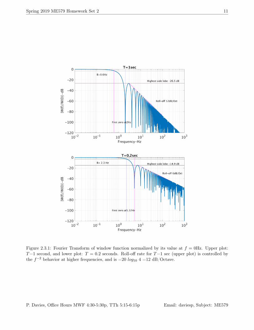
(c) See the two windows in Figure 2.3.1.



Figure 2.3.1: Fourier Transform of window function normalized by its value at f = 0Hz. Upper plot:T=1 second, and lower plot: T = 0.2 seconds. Roll-off rate for T=1 sec (upper plot) is controlled bythe f−2 behavior at higher frequencies, and is =20 log10 4 =12 dB/Octave.



(d) The roll-off of a rectangular window is 6dB per Octave, the highest side lobe is at -13dB and thefirst zero crossing is at 1

THz.

For the case where T=1, where the window is a simple triangle, the roll-off is controlled by thef2 in the denominator, and so the roll-off will be 12 dB per Octave. From the plot, we see thatthe highest side lobe is at -26.5 dB (much lower than the first lobe of the rectangular window)and the first zero crossing is at 2

T = 2 Hz, giving a wider main lobe that for the rectangular window.

The case where T=0.2 seconds is much more complicated because we have a combination of boththe rectangular and the triangular window. At higher frequencies the roll-off rate will be similarto that of a rectangular window with the sinc function still contributing strongly while the 1

f2in

the sinc2 function means that term’s contributions will be much smaller. The rectangular windowcontributes 0.8 to the height of the window and the triangular part contributes only 0.2 to theheight of the window, so the rectangular contributions will be strong even at low frequencies. Thefirst zero crossing is at 2

T=5.32 Hz, the rectangular window part, would have the first zero crossingat f = 1

0.2=5 Hz, so here we can see that the triangular part of the window is affecting the result.The height of the 1st side lobe is -14.9dB, just a little lower than that of a rectangular window.

(e) See part (d) and the 2.3.1.

Matlab Code

%h2q3.m%T=[1 0.2];f=logspace(-2,3,2000);

for kk=1:2;

W=T(kk)*(1-T(kk))*sinc(f*T(kk)) + T(kk)*(T(kk)/2)*sinc(f*T(kk)/2).^2;W0=T(kk)*(1-T(kk)) + ((T(kk)^2)/2)

P=20*log10(abs(W/W0));hold offmyplot(f,P,3,1,2,1,kk,’Frequency-Hz’,’|W(f)/W(0)|-dB’,[’T=’ num2str(T(kk)) ’sec’])xx=axis; xx=[0.01, 1000, -120, 0]; axis(xx);

if ( kk == 1)% Annotate graphshold onplot([xx(1) xx(2)],[-26.5 -26.5],’r’,[3/T(kk) 32*3/T(kk)],[-26.5 -86.5],’m’)plot([xx(1) xx(2)],[-3 -3],’k’);plot([2/T(kk) 2/T(kk)],[xx(3) xx(4)],’b’);plot([0.6/T(kk) 0.6/T(kk)],[xx(3) xx(4)],’m’)text(20,-22,’Highest side lobe -26.5 dB’)text(50,-60,’Roll-off 12dB/Oct’)text(0.1, -10,[’B=’ num2str(0.6/T(kk)) ’Hz’])text(0.5, -100,[’First zero at’ num2str(2/T(kk)) ’Hz’])elseif (kk == 2)



hold onplot([xx(1) xx(2)],[-14.9 -14.9],’r’,[7 32*7],[-14. -44],’m’)plot([xx(1) xx(2)],[-3 -3],’k’);plot([2.3 2.3],[xx(3) xx(4)],’b’);plot([5.32, 5.32],[xx(3), xx(4)],’m’);text(20,-12,’Highest side lobe -14.9 dB’)text(100,-30,’Roll-off 6dB/Oct’)text(0.1, -10,[’B= 2.3 Hz’])text(0.5, -100,[’First zero at’ num2str(5.32) ’Hz’])end

endprint -djpeg -r800 fig_h2_q3_1____________________________________________________Updated myplot.m

%myplot(f,P,1,1,1,2,kk,’Frequency-Hz’,’|W(f)/W(0)|-dB’,ti)% x - usually time or frequency% y - usually a time history or part of a spectrum% id - plot type: 1, regular, 2 = stem, 3 = semilogx% 4 - semilogy, 5-loglog, other=plot currently% ifig - figure number% a,b,c is subplot identification, e.g., subplot(a,b,c);% xlab - xlabel% ylab - ylabel% ti - titlefunction [] = myplot(x,y,id,ifig,a,b,c,xlab,ylab,ti)figure(ifig); orient tall; subplot(a,b,c);if (id == 2)stem(x,y);elseif (id == 1)plot(x,y);elseif(id == 3 )semilogx(x,y)elseif(id == 4 )semilogy(x,y)elseif(id == 5 )loglog(x,y)elseplot(x,y)end

grid on; xlabel(xlab); ylabel(ylab); title(ti);% Make fonts larger and lines thicker:vividoc(14,1.5)



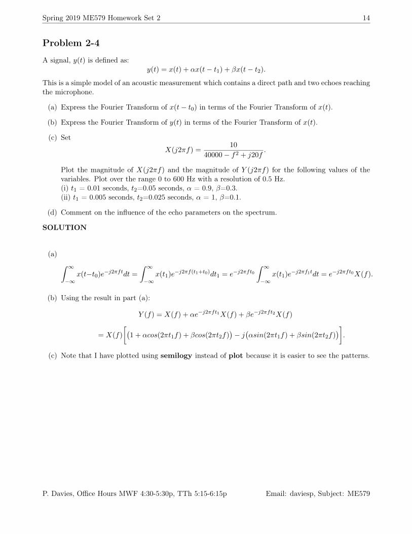
Problem 2-4

A signal, y(t) is defined as:y(t) = x(t) + αx(t− t1) + βx(t− t2).

This is a simple model of an acoustic measurement which contains a direct path and two echoes reachingthe microphone.

(a) Express the Fourier Transform of x(t− t0) in terms of the Fourier Transform of x(t).

(b) Express the Fourier Transform of y(t) in terms of the Fourier Transform of x(t).

(c) Set

X(j2πf) =10

40000− f2 + j20f.

Plot the magnitude of X(j2πf) and the magnitude of Y (j2πf) for the following values of thevariables. Plot over the range 0 to 600 Hz with a resolution of 0.5 Hz.(i) t1 = 0.01 seconds, t2=0.05 seconds, α = 0.9, β=0.3.(ii) t1 = 0.005 seconds, t2=0.025 seconds, α = 1, β=0.1.

(d) Comment on the influence of the echo parameters on the spectrum.

SOLUTION

(a) ∫ ∞−∞

x(t−t0)e−j2πftdt =

∫ ∞−∞

x(t1)e−j2πf(t1+t0)dt1 = e−j2πft0

∫ ∞−∞

x(t1)e−j2πf1tdt = e−j2πft0X(f).

(b) Using the result in part (a):

Y (f) = X(f) + αe−j2πft1X(f) + βe−j2πft2X(f)

= X(f)

[(1 + αcos(2πt1f) + βcos(2πt2f)

)− j(αsin(2πt1f) + βsin(2πt2f)

)].

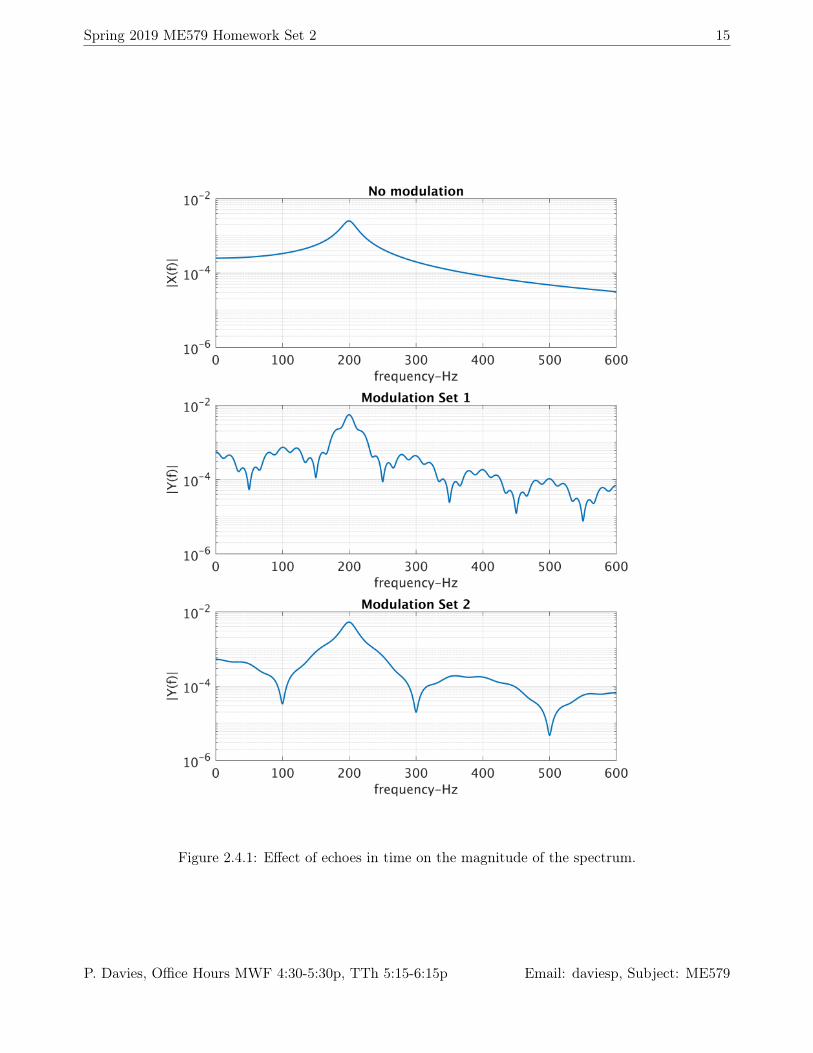
(c) Note that I have plotted using semilogy instead of plot because it is easier to see the patterns.



Figure 2.4.1: Effect of echoes in time on the magnitude of the spectrum.



(d) The echoes in the time history introduce modulations in the spectrum. We can see the reason forthis if we take the squared magnitude of Y (f):

|Y (f)|2 = |X(f)|2[1 + α2 + β2 + 2αcos(2πt1f) + 2βcos(2πt2f) + 2αβcos(2π(t1 − t2)f)

].

The period of the modulations in the spectrum are 1ti

and the depths of the modulations arecontrolled by α and by β.

(i) 1t1

= 100 Hz, and 1t2

= 20 Hz.(ii) 1

t1= 200 Hz, and 1

t2= 40 Hz.

When compared to case (i) the first component in case (ii) is a little bit stronger (1 vs 0.9) andthe second is much weaker (0.1 vs 0.3). So the second faster modulation is difficult to see. Thethird modulation component has a period of 1

t1−t2 but its amplitude is much smaller because ofthe product: αβ.

Matlab Code:

% h2q4.m%f=(0:0.5:600);t_1=[0.01 0.005]; t_2=[0.05 0.025]; al=[0.9 1]; be=[0.3 0.1];

Xf=10./(40000 - f.^2 +j*20*f);XfA = abs(Xf);

myplot(f,XfA,4,1,3,1,1,’frequency-Hz’,’|X(f)|’,’No modulation’)xx=axis; xx(3)=0.000001; xx(4)=0.01; axis(xx);

for ii=1:2Modu=1+al(ii)*exp(-j*2*pi*f*t_1(ii)) + be(ii)*exp(-j*2*pi*f*t_2(ii));XfMA=XfA.*abs(Modu);

myplot(f,XfMA,4,1,3,1,ii+1,’frequency-Hz’,’|Y(f)|’,[’Modulation Set ’ int2str(ii)])xx=axis; xx(3)=0.000001; xx(4)=0.01; axis(xx);end

print -djpeg -r800 fig_h2_q4_1

See Problem 2.3 for an updated myplot.m function. I have added various other plot options in it.


problem 2-1 - engineering.purdue.edu · me 579 fourier methods in digital signal processing...

Documents