Zach  Savidge    ECO  465  3/5/2014    

Problem  Set  #4    

Problem  1.      1a.    %define variables S=52;K=50;r= .05; dy = .05; t=1/2;num_steps=125;dt=t/num_steps;sigma=.25; %calculate states and probability of up state u = (exp( (r-dy)*dt + sigma*sqrt(dt))); d = (exp( (r-dy)*dt - sigma*sqrt(dt))); p = (exp((r - dy)*dt) - d)/(u-d); %calculate stock price at each final node vec = [125:-1:0']; vec2= [0:1:125']; ST = S*(u.^vec).*(d.^vec2); %calculate call payoff at each node and probability of each node CPayoff = max (ST-K, 0); Qprob = binopdf( (num_steps: -1:0)', num_steps, p); Cprice =exp(-r*t) * (CPayoff*Qprob)  Call  price  =4.5679    1b.  %define variables S=52; K=50; r=.05; d=1.30; exdiv =3/12; t=1/2; num_steps=125; dt=t/num_steps;sigma=.25; %Value of prepaid forward F = S - d^(-r*exdiv); %volatility of prepaid forward sigmaF = sigma * (S/F); %calculate u and d coefficients and probability of up-state u = exp( (r*dt + sigmaF*sqrt(dt))); d = exp( (r*dt - sigmaF*sqrt(dt))); p = (exp((r*dt)) - d)/(u-d); %calculate price of prepaid at end of period vec = [125:-1:0']; vec2= [0:1:125']; FT = F*(u.^vec).*(d.^vec2);

CPayoff = max (FT-K, 0); Qprob = binopdf( (num_steps: -1:0)', num_steps, p); Cprice =exp(-r*t) * (CPayoff*Qprob)  Call  price  =  4.8092    Using  a  continuous  dividend  gave  a  price  that  was  4.5679/  4.8092-­‐1    =  5.02%  less  than  using  a  discrete  dividend.          1c.      %define variables S=52; K=50; r= .05; dy = .075; t=1/3; num_steps=125; dt=t/num_steps; sigma=.25; %calculate state coefficients and probabilities u = (exp( (r-dy)*dt + sigma*sqrt(dt))); d = (exp( (r-dy)*dt - sigma*sqrt(dt))); p = (exp((r - dy)*dt) - d)/(u-d); %calculate stock price in final nodes vec = [125:-1:0']; vec2= [0:1:125']; ST = S*(u.^vec).*(d.^vec2); %calculate call payouts and probabilities of payouts at final nodes CPayoff = max (ST-K, 0); Qprob = binopdf( (num_steps: -1:0)', num_steps, p); Cprice =exp(-r*t) * (CPayoff*Qprob) Call  price  =  3.7140  with  a  continuous  dividend        %define variables S=52;K=50;r=.05; d=1.30; exdiv =3/12;t=1/3; num_steps=125; dt=t/num_steps;sigma=.25; %Value of prepaid forward F = S - d^(-r*exdiv); %volatility of prepaid forward sigmaF = sigma * (S/F); %calculate u and d coefficients and probability of up-state u = exp( (r*dt + sigmaF*sqrt(dt))); d = exp( (r*dt - sigmaF*sqrt(dt))); p = (exp((r*dt)) - d)/(u-d);

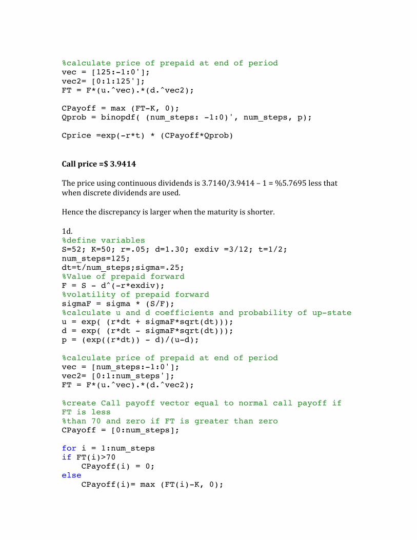
%calculate price of prepaid at end of period vec = [125:-1:0']; vec2= [0:1:125']; FT = F*(u.^vec).*(d.^vec2); CPayoff = max (FT-K, 0); Qprob = binopdf( (num_steps: -1:0)', num_steps, p); Cprice =exp(-r*t) * (CPayoff*Qprob)    Call  price  =$  3.9414    The  price  using  continuous  dividends  is  3.7140/3.9414  –  1  =  %5.7695  less  that  when  discrete  dividends  are  used.      Hence  the  discrepancy  is  larger  when  the  maturity  is  shorter.      1d.    %define variables S=52; K=50; r=.05; d=1.30; exdiv =3/12; t=1/2; num_steps=125; dt=t/num_steps;sigma=.25; %Value of prepaid forward F = S - d^(-r*exdiv); %volatility of prepaid forward sigmaF = sigma * (S/F); %calculate u and d coefficients and probability of up-state u = exp( (r*dt + sigmaF*sqrt(dt))); d = exp( (r*dt - sigmaF*sqrt(dt))); p = (exp((r*dt)) - d)/(u-d); %calculate price of prepaid at end of period vec = [num_steps:-1:0']; vec2= [0:1:num_steps']; FT = F*(u.^vec).*(d.^vec2); %create Call payoff vector equal to normal call payoff if FT is less %than 70 and zero if FT is greater than zero CPayoff = [0:num_steps]; for i = 1:num_steps if FT(i)>70 CPayoff(i) = 0; else CPayoff(i)= max (FT(i)-K, 0);

end end Qprob = binopdf( (num_steps: -1:0)', num_steps, p); Cprice =exp(-r*t) * (CPayoff*Qprob) Call  price  =  $3.7068          Problem  2    2a.    We  discount  the  expected  option  payout  at  the  risk  free  rate  because  we  are  using  the  risk-­‐neutral  probability  of  each  option  payout  instead  of  its  true  probability.  If  we  were  to  determine  the  true  probability  of  each  stock  price,  and  hence  each  option  payout,  on  a  binomial  tree,  we  would  then  discount  by  an  appropriate  discount  rate  reflecting  the  fact  that  an  option  is  a  leveraged  investment  in  the  stock.  It  can  be  shown  mathematically  that  both  these  methods  produce  the  same  valuation  for  the  option,  so  the  more  simple,  risk-­‐neutral  method  is  typically  used.      2b.  A  difference  between  the  borrowing  and  lending  rate  would  lead  to  a  no-­‐arbitrage  band,  instead  of  a  singular  price  at  which  the  call  price  could  not  be  arbitraged.  Any  price  within  this  band  is  a  feasible  price  for  the  call.      To  calculate  this  band,  we  use  the  binomial  options  pricing  model,  first  setting  the  risk  free  rate  equal  to  the  borrowing  rate,  9%:    

Δ =20− 0

41(1.4634− .7317) = 2/3  

𝐵! = 𝑒!.!"1.4634 ∗ 0− .7317 ∗ 20

1.4634− .7317 = −18.2786    Hence  the  price  of  the  call  cannot  be  more  than  𝐶 = !

!∗ 41− 18.2786 = $9.0547,  or  

a  market  participant  would  go  short  the  call  and  offset  it  by  borrowing  money  and  longing  the  stock  to  lock  in  an  arbitrage  profit.      Next,  we  apply  the  binomial  pricing  model,  setting  the  risk  free  rate  equal  to  the  lending  rate.      

𝐵! = 𝑒!.!"1.4634 ∗ 0− .7317 ∗ 20

1.4634− .7317 = −18.6479  

Likewise,  the  price  for  the  call  cannot  be  less  than  𝐶 = !!∗ 41− 18.6479 = $8.6854  

or  a  market  participant  would  go  long  the  call  and  hedge  the  position  by  shorting  the  stock  and  lending  money.      So  a  reasonable  band  for  the  call  price  is  $8.6854  to  $9.0547    2c.  If  we  assume  the  investor  has  other  taxable  income,  losses  are  tax  deductible  and  hence  actually  have  a  tax  advantage.  Thus  the  economics  payout  in  the  down  state  for  the  stock  and  call  are:      

𝑉𝑎𝑙𝑢𝑒  𝑜𝑓  𝐶𝑎𝑙𝑙 = 𝐶! − 𝑡! 𝐶! − 𝐶  𝑉𝑎𝑙𝑢𝑒  𝑜𝑓  𝑆𝑡𝑜𝑐𝑘 = 𝑆! − 𝑡! 𝑆! − 𝑆  

Thus  we  can  create  a  system  of  two  equations:    Δ 𝑆! − 𝑡! 𝑆! − 𝑆 + 𝐵𝑒!" − 𝐵𝑒!" − 𝐵 𝑡! = 𝐶! − 𝑡! 𝐶! − 𝐶  

Δ 𝑆! − 𝑡! 𝑆! − 𝑆 + 𝐵𝑒!" − 𝐵𝑒!" − 𝐵 𝑡! = 𝐶! − 𝑡! 𝐶! − 𝐶    Solving  both  for  C  and  setting  them  equal  to  each  other  we  get:    

 Δ 𝑆! − 𝑡! 𝑆! − 𝑆 + 𝐵𝑒!" − 𝐵𝑒!" − 𝐵 𝑡! − 𝐶! + 𝑡! 𝐶!

𝑡!=Δ 𝑆! − 𝑡! 𝑆! − 𝑆 + 𝐵𝑒!" − 𝐵𝑒!" − 𝐵 𝑡! − 𝐶! + 𝑡! 𝐶!

𝑡!  

 Cancelling  terms  we  get:      

 

Δ 𝑆! − 𝑡! 𝑆! − 𝑆 − 𝐶! + 𝑡! 𝐶! =  Δ 𝑆! − 𝑡! 𝑆! − 𝑆 − 𝐶! + 𝑡! 𝐶!    Solving  for  delta  we  get:    

Δ =𝐶! 1− 𝑡! − 𝐶! 1− 𝑡!𝑆! 1− 𝑡! − 𝑆! 1− 𝑡!

=(𝐶! − 𝐶!) 1− 𝑡!𝑆(𝑢 − 𝑑) 1− 𝑡!

 

 By  no  arbitrage,  we  know  if  the  payouts  for  the  stock  and  bond  position  are  the  same  as  for  the  call,  the  price  to  enter  the  position  must  be  the  same  as  the  price  of  the  call:    

Δ𝑆 + 𝐵 = 𝐶    Thus  we  can  solve  for  B  by  plugging  our  delta  and  the  equation  above  back  into  one  of  our  original  equations:        

Δ 𝑆! − 𝑡! 𝑆! − 𝑆 + 𝐵𝑒!" − 𝐵𝑒!" − 𝐵 𝑡! = 𝐶! − 𝑡! 𝐶! − Δ𝑆 − 𝐵  𝐵𝑒!" − 𝐵𝑒!"𝑡! + 𝐵𝑡! + 𝐵𝑡! = 𝐶! − 𝑡!𝐶! + Δ(S𝑡! − 𝑑𝑆 + 𝑑𝑆𝑡! − 𝑆𝑡!)  𝐵 𝑒!" 1− 𝑡! + 𝑡! + 𝑡! = 𝐶! 1− 𝑡! + ΔS(𝑡! − 𝑡! − 𝑑 1− 𝑡! )  

 

Simplifying  this  expression  gives:    

𝐵 =1

𝑒!" ∗ 1− 𝑡!1− 𝑡!− 𝑡! − 𝑡!1− 𝑡!

∗ (𝑢𝐶! − 𝑑𝐶!𝑢 − 𝑑 −

Δ𝑆 ∗ 𝑡! − 𝑡!1− 𝑡! 1− 𝑡!

)  

 The  risk  neutral  probability  is  calculated  by  using  the  normal  formula  but  inserting  the  tax  

adjusted  risk  free  rate:  𝑝 =!!"∗!!!!!!!!

!!!!!!!!!!!!

!!!  

 When  the  three  tax  rates  are  set  equal  to  each  other,  they  cancel  from  the  above  equations  and  hence  do  not  affect  the  pricing  of  assets.  As  many  large  market  players  have  all  sources  of  income  taxed  at  the  same  rate,  in  practice  these  assets  can  be  priced  without  considering  the  tax  rate.      Problem  3    3a.  Asian  options  are  less  expensive  than  European  options  because  the  volatility  of  the  average  price  of  a  security  is  less  than  the  volatility  of  its  spot  price  and  the  price  of  an  option  increases  with  volatility.        3b.  The  question  is  somewhat  ambivalent  in  defining  the  strike  price.  I  interpret  the  question  to  mean  that  the  strike  price  is  equal  to  the  current  stock  price,  not  the  average  stock  price,    𝑒(!!!)! ,  hence  K  =  50.503.    The  option  takes  the  average  stock  prices  over  the  last  3  months,  but  because  we  are  only  constructing  a  15-­‐step  model,  this  time  frame  cannot  be  exactly  captured.  I  choose  to  take  the  average  over  the  last  8  nodes  to  best  capture  the  stock  price  in  the  last  3  months  before  expiration.        

%define variables S=50; r= .05; dy = .03; t=1/2; num_steps=15; dt=t/num_steps; sigma=.25; K =S*exp((r-dy)*t); %calculate state coefficients and probabilities u = (exp( (r-dy)*dt + sigma*sqrt(dt))); d = (exp( (r-dy)*dt - sigma*sqrt(dt))); p = (exp((r - dy)*dt) - d)/(u-d); %create a matrix of 1s and 0s with a row corresponding to each distinct %path the stock can take b =1; while length(b) ~= 2^num_steps x = binornd(1, .5, 1000000, num_steps); b = unique(x, 'rows');

end %set the 1s in the matrix to u and the 0s to d b = u.*b; for n = 1:2^num_steps; for i = 1:num_steps; if b(n,i)==0; b(n,i)=d; else b(n,i); end end end %multiply by the prepaid forward price to create a matrix of each dinstinct %path the stock can take. If the stock hits 70, set it equal to zero for the %remainder of the path. for n = 1:2^num_steps; b(n,1)=S*b(n,1); for i = 2:num_steps; b(n,i)=b(n,i)*b(n,i-1); end end %find the sum of the last 8 nodes in each distinct path and create a vector %of these sums SC = zeros(2^num_steps,1); for n = 1:2^num_steps; for i=8:num_steps; SC(n) = SC(n)+b(n,i); end end %find the average stock price over the last 8 nodes for each distinct path %from these sums SA=SC/8; %calculate the payoff of the option for each distinct path for n = 1:2^num_steps; Cpayoff(n) = max(SA(n) - K, 0); end %find the price of the call by summing the potential

payouts and dividing %them by the probability of any given distinct stock path Cprice = exp(-r*t) * sum(Cpayoff)*(1/(2^num_steps))

 Call  price  =  $3.1402    

   3c.  It  is  significantly  harder  to  value  because  it  is  path  dependent.      Below  is  MATLAB  code  for  valuing  this  option  assuming  it  has  the  same  characteristics  as  the  options  in  problem  1d.    The  price  of  the  call  comes  to  $4.0300    

%define variables S=52; K=50; r=.05; d=1.30; exdiv =3/12; t=1/2; num_steps=15; dt=t/num_steps;sigma=.25; %Value of prepaid forward F = S - d^(-r*exdiv); %volatility of prepaid forward sigmaF = sigma * (S/F); %calculate u and d coefficients and probability of up-state u = exp( (r*dt + sigmaF*sqrt(dt))); d = exp( (r*dt - sigmaF*sqrt(dt))); p = (exp((r*dt)) - d)/(u-d); %create a matrix of 1s and 0s with a row corresponding to each distinct %path the stock can take b =1; while length(b) ~= 2^num_steps x = binornd(1, .5, 1000000, num_steps); b = unique(x, 'rows'); end %set the 1s in the matrix to u and the 0s to d b = u.*b; for n = 1:2^num_steps; for i = 1:num_steps; if b(n,i)==0; b(n,i)=d; else b(n,i); end end

end %multiply by the prepaid forward price to create a matrix of each dinstinct %path the stock can take. If the stock hits 70, set it equal to zero for the %remainder of the path. for n = 1:2^num_steps; b(n,1)=F*b(n,1); for i = 2:num_steps; if b(n,i-1)>70 b(n,i)=0; else b(n,i)=b(n,i)*b(n,i-1); end end end %calculate the payoff of the option. Since we set the stock to 0 for all %paths which resulted in the stock going above 70, we can ignore this %feature of the call for n = 1:2^num_steps; Cpayoff(n) = max(b(n,num_steps) - K, 0); end %find the price of the call by summing the potential payouts and dividing %them by the probability of any given distinct stock path Cprice = exp(-r*t) * sum(Cpayoff)*(1/(2^num_steps))