problem set 6 solutions - college of...

MSE 508 Dept. of Materials Science & Engineering Solid State Thermodynamics Spring 2011/Bill Knowlton

1

Problem Set 6 Solutions 1. In class, we found that lnk kRT amD = . Using the toolbox 5 tables, derive Toolbox 5-

4 disregarding the first three and last listings in the tables. That is, derive the following:

Toolbox 5-4: Relations between the PMPs of component k and its activity

,

lnln

k

kk k

p n

aS R a RT

T

,

ln

k

kk

T n

aV RT

P

2

,

ln

k

kk

p n

aH RT

T

2

, ,

ln ln

k k

k kk

p n T n

a aU RT PRT

T P

,

lnln

k

kk k

T n

aF RT a PRT

P


2


3


4

2. In the system Pandemonium (Pn) – Condominium (Cn), the partial molar heat of mixing of Condominium (Cn) can be fitted by the expression: .

2 where 12,500Cn Pn Cn

JH aX X a

mole

.

Calculate and plot the function that describes the variation of the heat of mixing with composition for this system. In plotting the function, do so with a mathematical program that is not Excel. Do comment and provide insight to your plot.

units = J/mol


5

0.0 0.2 0.4 0.6 0.8 1.00

200

400

600

800

XCn

H m

ix

J mol

Hmix

0.0 0.2 0.4 0.6 0.8 1.00

200

400

600

800

XPn

H m

ix

J mol

Hmix

It is evident that from the equation describing the enthalpy of mixing, ∆Hmix =a/2(X2

CnXPn), is not of the form aXCnXPn and therefore does not describe a regular solution. Hence, the solution is non-, sub-, or irregular. This is also evident due to the lack of symmetry in the plot above. The solution is skewed toward larger values of Xcn (max. ~ 0.7Cn) since the mixture goes by XCn

2 and only linear in XPn. Notice that ∆Hmix has a positive maximum when the stoichiometry of the alloy is Cn2Pn. This means that the reaction for the solution at this stoichiometry is the most endothermic suggesting that this stoichiometry is the least likely to form. This may be due to a repulsive behavior between Cn-Cn. The entropy of the solution is not discussed here and will certainly have an effect on which stoichiometry will form. To determine whether or not the Cn2Pn alloy is the least likely to form requires knowledge of ∆Gmix.


6

3. Below is a thoroughly stated problem with a thoroughly provided solution. Create a a thoroughly problem and a thoroughly stated solution that parallels the problem and solution provided below. For the problem, you will either need to create your own data or find data (the literature: text books, journal articles, etc.). Be as thorough as the problem and solution is below.

PROBLEM: Data are given below for the xs

mixG as a function of composition for a liquid

solution of Fe and Mn at 1863 K. Using the data, thoroughly answer the following questions and comment and provide insight to each of the thoroughly labeled plots that you generate: XMn 0.1 0.2 0.3 0.4 0.5 0.6 0.7 0.8 0.9

xsmixG (J/mol) 395 703 925 1054 1100 1054 925 703 395

a. Prove whether or not the system exhibits regular solution behavior.

For this problem, much insight to the regular solution model can be gained from:

[1] Joel H. Hildebrand, Solubility. XII. Regular Solutions, Journal of the American Chemical Society, 51 (1929) p. 66-80. You can ask Bill for a copy. Let: X1=XMn and X2=XFe

Note: The regular solution model is defined in Toolbox 5-2 at the bottom of column 1. Using this information, we can prove whether or not the data in the above table exhibits Regular Solution Behavior.


7

Note that ao should be J/mole and the same is true for xs

mixG .


8

For the remainder of the problem, let: XS = regular solution XS

b. Derive an equation for xsmixG and plot it as a function of XMn. Explain

whether or not the plot exhibits endothermic or exothermic behavior and provide insight as to why this behavior is observed.

Since the solution is regular, we know that the regular solution model is defined in Toolbox 5-2 at the bottom of column 1 such that:

2 21 22 1

2 2

&

&

xs xs

o o

xs xsMn Feo Fe o Mn

G a X G a X

G a X G a X

[1].

where X1=XMn and X2=XFe. In general, we know from toolbox 5-1 that: 1 21 2

xs xsxsmixG X G X G [2]

And substituting [1] into [2], we find that:

2 21 2 2 1

1 2 2 1

1 2

xsmix o o

o

o

o Mn Fe

G X a X X a X

a X X X X

a X X

a X X

The answer above is no surprise since it is of the same form as shown for the regular solution model in Toolbox 5-2 at the bottom of column 1. We know ao is 4395 J/mole and we can now plot xs

mixG .

0 0.2 0.4 0.6 0.8 1XMn

200

400

600

800

1000

1200

G

ximsx

J lom

Gmixxs

Since xs xs

mix mix mixG H H and we see that the curve is positive in energy, then we can say that the curve exhibits endothermic behavior.


9

c. Derive equations for xsFeG and

xsMnG and plot them as a function of XMn.

Comment and provide insight for your plot. From part a, we know that:

2 2 & xs xsMn Feo Fe o MnG a X G a X [1].

We know ao is 4395 J/mole and we can now plot xsFeG and

xsMnG .

0 0.2 0.4 0.6 0.8 1XMn

0

1000

2000

3000

4000G

ksx

J

lom

Blue : G1xs; Red: G2

xs

What we see is that as 0,

xsMnMn oX G a and becomes very active and does

not act ideal at all. This makes sense since there is very little Mn in solution and is probably being solvated by Fe and vice versa. We also observe that as

1, 0 & xs IDMn Mn MnMnX G G G . So pure Mn or pure Fe acts as an ideal

solution in this regime.

d. Derive an equation for mixS and plot as a function of XMn. Comment on

and provide sight to your plot. Since the solution is regular, we know that:

Reg ID1 1 2 2ln ln ln lnmix mix Mn Mn Fe FeS S R X X X X R X X X X

0 0.2 0.4 0.6 0.8 1XMn

1

2

3

4

5

6

S

ximgeR

J

lom

SmixReg

We observe that at maximum mixing where XMn = XFe = 0.5 that the solution is at its greatest disorder thereby maximizing entropy.


10

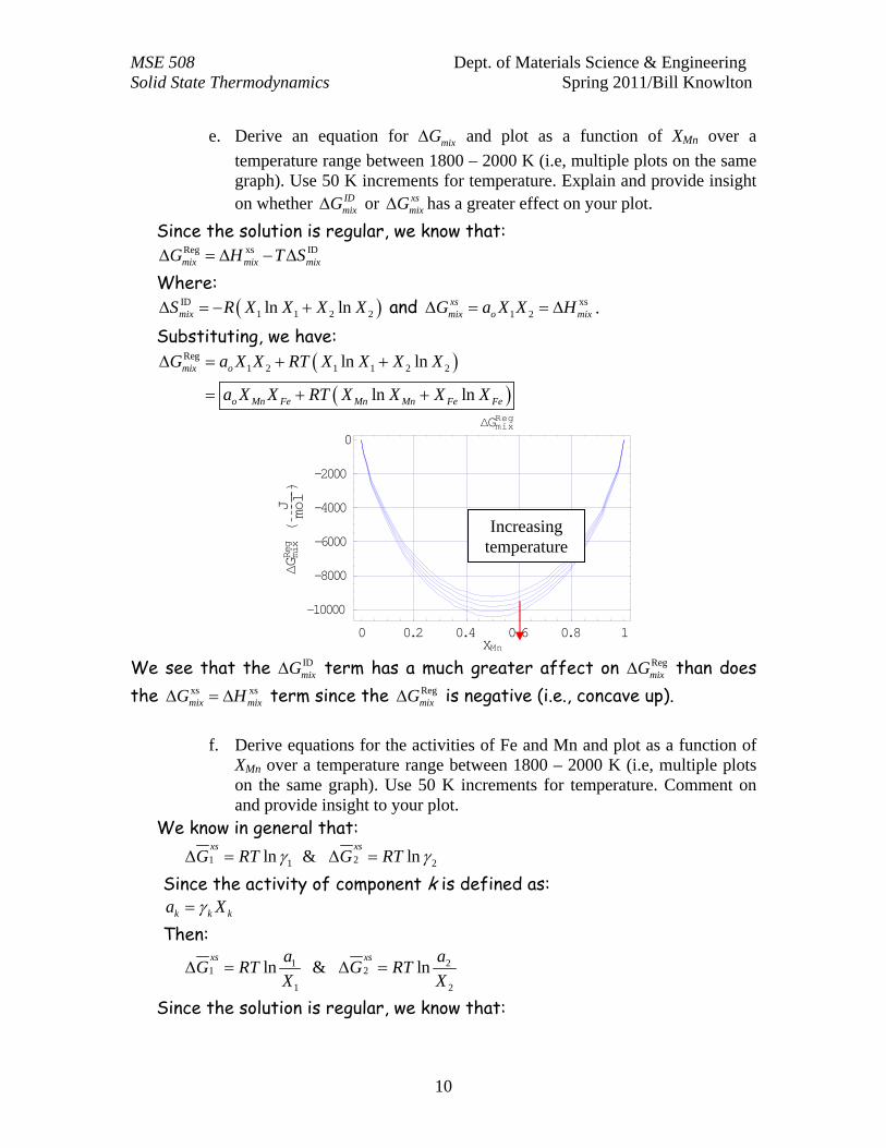
e. Derive an equation for mixG and plot as a function of XMn over a

temperature range between 1800 – 2000 K (i.e, multiple plots on the same graph). Use 50 K increments for temperature. Explain and provide insight on whether ID

mixG or xsmixG has a greater effect on your plot.

Since the solution is regular, we know that: Reg xs IDmix mix mixG H T S

Where: ID

1 1 2 2ln lnmixS R X X X X and xs1 2

xsmix o mixG a X X H .

Substituting, we have:

Reg1 2 1 1 2 2ln ln

ln ln

mix o

o Mn Fe Mn Mn Fe Fe

G a X X RT X X X X

a X X RT X X X X

0 0.2 0.4 0.6 0.8 1XMn

-10000

-8000

-6000

-4000

-2000

0

G

ximgeR

J

lom

GmixReg

We see that the ID

mixG term has a much greater affect on RegmixG than does

the xs xsmix mixG H term since the Reg

mixG is negative (i.e., concave up).

f. Derive equations for the activities of Fe and Mn and plot as a function of XMn over a temperature range between 1800 – 2000 K (i.e, multiple plots on the same graph). Use 50 K increments for temperature. Comment on and provide insight to your plot.

We know in general that: 1 21 2ln & lnxs xs

G RT G RT

Since the activity of component k is defined as: k k ka X

Then: 1 2

1 2

1 2

ln & lnxs xsa a

G RT G RTX X

Since the solution is regular, we know that:

Increasing temperature


11

2 21 22 1 & xs xs

o oG a X G a X Equating the last two sets of equations, we have:

2 21 22 1

1 2

ln & lno o

a aRT a X RT a X

X X

Solving for the activities, we have:

2 2 2 22 2

222

1 1 2

1-1-

2 2

1- so 1-

so

o o o Fe o Fe

o Feo

a X a X a X a X

RT RT RT RTMn Mn Fe

a Xa X

RT RTFe Fe

a X e X e a X e X e

a X e a X e

0 0.2 0.4 0.6 0.8 1XMn

0

0.2

0.4

0.6

0.8

1

a k

aFeGreen & aMnMagenta

We see that the activity does not vary greatly as a function of temperature. Since

xskG for regular solution is not, to first order, a

function of temperature (see [1]), this result is not too surprising.


12

g. Derive equations for the activity coefficients of Fe and Mn and plot as a function of XMn over a temperature range between 1800 – 2000 K (i.e, multiple plots on the same graph). Use 50 K increments for temperature. Comment on and provide insight to your plot.

We know in general that: 1 21 2ln & lnxs xs

G RT G RT

Since the solution is regular, we know that: 2 2

1 22 1 & xs xs

o oG a X G a X Equating the last two sets of equations, we have:

2 21 2 2 1ln & lno oRT a X RT a X

Solving for the activities, we have:

2 22

222

1

1-1-

2

so

so

o o Fe

o Feo

a X a X

RT RTMn

a Xa X

RT RTFe

e e

e e

0 0.2 0.4 0.6 0.8 1XMn

1

1.05

1.1

1.15

1.2

1.25

1.3

k

FeOrange & MnPurple

We observe that for a solution of near purity, the for the solute approaches 1 with little effect by temperature. This signifies a near ideal solution case. As the solute concentration becomes very dilute, the increases but less so with increasing temperature. However, temperature has little effect as we would expect since xs

mixS must be zero for a regular

solution. Thus, 1 2 and xs xs

S S must be zero. That is, ,

0

k

xsxs kk

P n

GS

T

. As

mentioned in part f, since xskG for regular solution is not, to first order, a

function of temperature (see [1]), this result is not too surprising.

Increasing temperature

problem set 6 solutions - college of...

Documents