proceedings e report 90 · 2021. 5. 5. · ecos 2012 : the 25 th international conference on...

Proceedings e report

90

ECOS 2012The 25th International Conference on Efficiency, Cost, Optimization and Simulation of Energy Conversion

Systems and Processes (Perugia, June 26th-June 29th, 2012)

edited byUmberto Desideri, Giampaolo Manfrida,

Enrico Sciubba

firenze university press2012

Peer Review ProcessAll publications are submitted to an external refereeing process under the responsibility of the FUP Editorial Board and the Scientific Committees of the individual series. The works published in the FUP catalogue are evaluated and approved by the Editorial Board of the publishing house. For a more detailed description of the refereeing process we refer to the official documents published on the website and in the online catalogue of the FUP (http://www.fupress.com).

Firenze University Press Editorial BoardG. Nigro (Co-ordinator), M.T. Bartoli, M. Boddi, F. Cambi, R. Casalbuoni, C. Ciappei, R. Del Punta, A. Dolfi, V. Fargion, S. Ferrone, M. Garzaniti, P. Guarnieri, G. Mari, M. Marini, M. Verga, A. Zorzi.

© 2012 Firenze University PressUniversità degli Studi di FirenzeFirenze University PressBorgo Albizi, 28, 50122 Firenze, Italyhttp://www.fupress.com/Printed in Italy

Progetto grafico di copertina Alberto Pizarro, Pagina Maestra sncImmagine di copertina: © Kts | Dreamstime.com

ECOS 2012 : the 25th International Conference on Efficiency, Cost, Optimization and Simulation of Energy Conversion Systems and Processes (Perugia, June 26th-June 29th, 2012) / edited by Umberto Desideri, Giampaolo Manfrida, Enrico Sciubba. – Firenze : Firenze University Press, 2012.(Proceedings e report ; 90)

http://digital.casalini.it/9788866553229

ISBN 978-88-6655-322-9 (online)

ECOS 2012 - THE 25TH INTERNATIONAL CONFERENCE ON EFFICIENCY, COST, OPTIMIZATION, SIMULATION AND ENVIRONMENTAL IMPACT OF ENERGY SYSTEMS

JUNE 26-29, 2012, PERUGIA, ITALY EDITED BY UMBERTO DESIDERI, GIAMPAOLO MANFRIDA, ENRICO SCIUBBA

FIRENZE UNIVERSITY PRESS, 2012, ISBN ONLINE : 978-88-6655-322-9

ECOS 2012

The 25th International Conference on

Efficiency, Cost, Optimization and Simulation of Energy Conversion Systems and Processes

Perugia, June 26th-June 29th, 2012

Book of Proceedings - Volume IV

Edited by: Umberto Desideri, Università degli Studi di Perugia Giampaolo Manfrida, Università degli Studi di Firenze Enrico Sciubba, Università degli Studi di Roma “Sapienza”

iii

Advisory Committee (Track Organizers) Building, Urban and Complex Energy Systems V. Ismet Ugursal Dalhousie University, Nova Scotia, Canada Combustion, Chemical Reactors, Carbon Capture and Sequestration Giuseppe Girardi ENEA-Casaccia, Italy Energy Systems: Environmental and Sustainability Issues Christos A. Frangopoulos National Technical University of Athens, Greece Exergy Analysis and Second Law Analysis Silvio de Oliveira Junior Polytechnical University of Sao Paulo, Sao Paulo, Brazil Fluid Dynamics and Power Plant Components Sotirios Karellas National Technical University of Athens, Athens, Greece Fuel Cells Umberto Desideri University of Perugia, Perugia, Italy Heat and Mass Transfer Francesco Asdrubali, Cinzia Buratti University of Perugia, Perugia, Italy Industrial Ecology Stefan Goessling-Reisemann University of Bremen, Germany Poster Session Enrico Sciubba University Roma 1 “Sapienza”, Italy Process Integration and Heat Exchanger Networks Francois Marechal EPFL, Lausanne, Switzerland Renewable Energy Conversion Systems David Chiaramonti University of Firenze, Firenze, Italy Simulation of Energy Conversion Systems Marcin Liszka Polytechnica Slaska, Gliwice, Poland System Operation, Control, Diagnosis and Prognosis Vittorio Verda Politecnico di Torino, Italy Thermodynamics A. Özer Arnas United States Military Academy at West Point, U.S.A. Thermo-Economic Analysis and Optimisation Andrea Lazzaretto University of Padova, Padova, Italy Water Desalination and Use of Water Resources Corrado Sommariva ILF Consulting M.E., U.K

iv

Scientific Committee Riccardo Basosi, University of Siena, Italy Gino Bella, University of Roma Tor Vergata, Italy Asfaw Beyene, San Diego State University, United States Ryszard Bialecki, Silesian Institute of Tecnology, Poland Gianni Bidini, University of Perugia, Italy Ana M. Blanco-Marigorta, University of Las Palmas de Gran Canaria, Spain Olav Bolland, University of Science and Technology (NTNU), Norway Renè Cornelissen, Cornelissen Consulting, The Netherlands Franco Cotana, University of Perugia, Italy Alexandru Dobrovicescu, Polytechnical University of Bucharest, Romania Gheorghe Dumitrascu, Technical University of Iasi, Romania Brian Elmegaard, Technical University of Denmark , Denmark Daniel Favrat, EPFL, Switzerland Michel Feidt, ENSEM - LEMTA University Henri Poincaré, France Daniele Fiaschi, University of Florence, Italy Marco Frey, Scuola Superiore S. Anna, Italy Richard A Gaggioli, Marquette University, USA Carlo N. Grimaldi, University of Perugia, Italy Simon Harvey, Chalmers University of Technology, Sweden Hasan Heperkan, Yildiz Technical University, Turkey Abel Abel Hernandez-Guerrero, University of Guanajuato, Mexico Jiri Jaromir Klemeš, University of Pannonia, Hungary Zornitza V. Kirova-Yordanova, University "Prof. Assen Zlatarov", Bulgaria Noam Lior, University of Pennsylvania, United States Francesco Martelli, University of Florence, Italy Aristide Massardo, University of Genova, Italy Jim McGovern, Dublin Institute of Technology, Ireland Alberto Mirandola, University of Padova, Italy Michael J. Moran, The Ohio State University, United States Tatiana Morosuk, Technical University of Berlin, Germany Pericles Pilidis, University of Cranfield, United Kingdom Constantine D. Rakopoulos, National Technical University of Athens, Greece Predrag Raskovic, University of Nis, Serbia and Montenegro Mauro Reini, University of Trieste, Italy Gianfranco Rizzo, University of Salerno, Italy Marc A. Rosen, University of Ontario, Canada Luis M. Serra, University of Zaragoza, Spain Gordana Stefanovic, University of Nis, Serbia and Montenegro Andrea Toffolo, Luleå University of Technology, Sweden Wojciech Stanek, Silesian University of Technology, Poland George Tsatsaronis, Technical University Berlin, Germany Antonio Valero, University of Zaragoza, Spain Michael R. von Spakovsky, Virginia Tech, USA Stefano Ubertini, Parthenope University of Naples, Italy Sergio Ulgiati, Parthenope University of Naples, Italy Sergio Usón, Universidad de Zaragoza, Spain Roman Weber, Clausthal University of Technology, Germany Ryohei Yokoyama, Osaka Prefecture University, Japan Na Zhang, Institute of Engineering Thermophysics, Chinese Academy of Sciences, China

vi

The 25th ECOS Conference 1987-2012: leaving a mark The introduction to the ECOS series of Conferences states that “ECOS is a series of international conferences that focus on all aspects of Thermal Sciences, with particular emphasis on Thermodynamics and its applications in energy conversion systems and processes”. Well, ECOS is much more than that, and its history proves it!

The idea of starting a series of such conferences was put forth at an informal meeting of the Advanced Energy Systems Division of the American Society of Mechanical Engineers (ASME) at the November 1985 Winter Annual Meeting (WAM), in Miami Beach, Florida, then chaired by Richard Gaggioli. The resolution was to organize an annual Symposium on the Analysis and Design of Thermal Systems at each ASME WAM, and to try to involve a larger number of scientists and engineers worldwide by organizing conferences outside of the United States. Besides Rich other participants were Ozer Arnas, Adrian Bejan, Yehia El-Sayed, Robert Evans, Francis Huang, Mike Moran, Gordon Reistad, Enrico Sciubba and George Tsatsaronis.

Ever since 1985, a Symposium of 8-16 sessions has been organized by the Systems Analysis Technical Committee every year, at the ASME Winter Annual Meeting (now ASME-IMECE). The first overseas conference took place in Rome, twenty-five years ago (in July 1987), with the support of the U.S. National Science Foundation and of the Italian National Research Council. In that occasion, Christos Frangopoulos, Yalcin Gogus, Elias Gyftopoulos, Dominick Sama, Sergio Stecco, Antonio Valero, and many others, already active at the ASME meetings, joined the core-group.

The name ECOS was used for the first time in Zaragoza, in 1992: it is an acronym for Efficiency, Cost, Optimization and Simulation (of energy conversion systems and processes), keywords that best describe the contents of the presentations and discussions taking place in these conferences. Some years ago, Christos Frangopoulos inserted in the official website the note that “ècos” (’ ) means “home” in Greek and it ought to be attributed the very same meaning as the prefix “Eco-“ in environmental sciences. The last 25 years have witnessed an almost incredible growth of the ECOS community: more and more Colleagues are actively participating in our meetings, several international Journals routinely publish selected papers from our Proceedings, fruitful interdisciplinary and international cooperation projects have blossomed from our meetings. Meetings that have spanned three continents (Africa and Australia ought to be our next targets, perhaps!) and influenced in a way or another much of modern Engineering Thermodynamics. After 25 years, if we do not want to become embalmed in our own success and lose momentum, it is mandatory to aim our efforts in two directions: first, encourage the participation of younger academicians to our meetings, and second, stimulate creative and useful discussions in our sessions. Looking at this years’ registration roster (250 papers of which 50 authored or co-authored by junior Authors), the first objective seems to have been attained, and thus we have just to continue in that direction; the second one involves allowing space to “voices that sing out of the choir”, fostering new methods and approaches, and establishing or reinforcing connections to other scientific communities. It is important that our technical sessions represent a place of active confrontation, rather than academic “lecturing”. In this spirit, we welcome you in Perugia, and wish you a scientifically stimulating, touristically interesting, and culinarily rewarding experience. In line with our 25 years old scientific excellency and friendship! Umberto Desideri, Giampaolo Manfrida, Enrico Sciubba

vii

CONTENT MANAGEMENT

The index lists all the papers contained all the eight volumes of the Proceedings of the

ECOS 2012 International Conference. Page numbers are listed only for papers within the Volume you are looking at.

The ID code allows to trace back the identification number assigned to the paper within the Conference submission, review and track organization processes.

-------------------------------------------------------------------------------------------------- ECOS 2012 - THE 25TH INTERNATIONAL CONFERENCE ON

EFFICIENCY, COST, OPTIMIZATION, SIMULATION AND ENVIRONMENTAL IMPACT OF ENERGY SYSTEMS JUNE 26-29, 2012, PERUGIA, ITALY

EDITED BY UMBERTO DESIDERI, GIAMPAOLO MANFRIDA, ENRICO SCIUBBA FIRENZE UNIVERSITY PRESS, 2012, ISBN ONLINE : 978-88-6655-322-9

CONTENT VOLUME IV

IV. 1 FLUID DYNAMICS AND POWER PLANT COMPONENTS

» A control oriented simulation model of a multistage axial compressor (ID 444) Lorenzo Damiani, Giampaolo Crosa, Angela Trucco

…….... Pag. 1

» A flexible and simple device for in-cylinder flow measurements: experimental and numerical validation (ID 181) Andrea Dai Zotti, Massimo Masi, Marco Antonello

…….... Pag. 15

» CFD Simulation of Entropy Generation in Pipeline for Steam Transport in Real Industrial Plant (ID 543) Goran Vu kovi , Gradimir Ili , Mi a Vuki , Milan Bani , Gordana Stefanovi

…….... Pag. 36

» Feasibility Study of Turbo expander Installation in City Gate Station (ID 168) Navid Zehtabiyan Rezaie, Majid Saffar-Avval

…….... Pag. 47

» GTL and RME combustion analysis in a transparent CI engine by means of IR digital imaging (ID 460) Ezio Mancaruso, Luigi Sequino, Bianca Maria Vaglieco

…….... Pag. 56

» Some aspects concerning fluid flow and turbulence modeling in 4-valve engines (ID 116) Zoran Stevan Jovanovic, Zoran Masonicic, Miroljub Tomic

…….... Pag. 66

IV. 2 SYSTEM OPERATION CONTROL DIAGNOSIS AND PROGNOSIS

» Adapting the operation regimes of trigeneration systems to renewable energy systems integration (ID 188) Liviu Ruieneanu, Mihai Paul Mircea

…….... Pag. 82

» Advanced electromagnetic sensors for sustainable monitoring of industrial processes (ID 145) Uroš Puc, Andreja Abina, Anton Jegli , Pavel Cevc, Aleksander Zidanšek

…….... Pag. 92

» Assessment of stresses and residual life of plant components in view of life-time extension of power plants (ID 453) Anna Stoppato, Alberto Benato and Alberto Mirandola

…….... Pag. 104

» Control strategy for minimizing the electric power consumption of hybrid ground source heat pump system (ID 244) Zoi Sagia, Constantinos Rakopoulos

…….... Pag. 114

» Exergetic evaluation of heat pump booster configurations in a low temperature district heating network (ID 148) Torben Ommen, Brian Elmegaard

…….... Pag. 126

» Exergoeconomic diagnosis: a thermo-characterization method by using irreversibility analysis (ID 523) Abraham Olivares-Arriaga, Alejandro Zaleta-Aguilar, Rangel-Hernández V. H, Juan Manuel Belman-Flores

…….... Pag. 140

» Optimal structural design of residential cogeneration systems considering their operational restrictions (ID 224) Tetsuya Wakui, Ryohei Yokoyama

…….... Pag. 156

ix

» Performance estimation and optimal operation of a CO2 heat pump water heating system (ID 344) Ryohei Yokoyama, Ryosuke Kato, Tetsuya Wakui, Kazuhisa Takemura

…….... Pag. 173

» Performances of a common-rail Diesel engine fuelled with rapeseed and waste cooking oils (ID 213) Alessandro Corsini, Valerio Giovannoni, Stefano Nardecchia, Franco Rispoli, Fabrizio Sciulli, Paolo Venturini

…….... Pag. 188

» Reduced energy cost through the furnace pressure control in power plants (ID 367) Vojislav Filipovi , Novak Nedi , Saša Prodanovi

…….... Pag. 203

» Short-term scheduling model for a wind-hydro-thermal electricity system (ID 464) Sérgio Pereira, Paula Ferreira, A. Ismael Freitas Vaz

…….... Pag. 212

-----------------------------------------------------------------------

CONTENTS OF ALL THE VOLUMES

-----------------------------------------------------------------------

VOLUME I

I . 1 - SIMULATION OF ENERGY CONVERSION SYSTEMS

» A novel hybrid-fuel compressed air energy storage system for China’s situation (ID 531) Wenyi Liu, Yongping Yang, Weide Zhang, Gang Xu,and Ying Wu

» A review of Stirling engine technologies applied to micro-cogeneration systems (ID 338) Ana C Ferreira, Manuel L Nunes, Luís B Martins, Senhorinha F Teixeira

» An organic Rankine cycle off-design model for the search of the optimal control strategy (ID 295) Andrea Toffolo, Andrea Lazzaretto, Giovanni Manente, Marco Paci

» Automated superstructure generation and optimization of distributed energy supply systems (ID 518) Philip Voll, Carsten Klaffke, Maike Hennen, André Bardow

» Characterisation and classification of solid recovered fuels (SRF) and model development of a novel thermal utilization concept through air- gasification (ID 506) Panagiotis Vounatsos, Konstantinos Atsonios, Mihalis Agraniotis, Kyriakos D. Panopoulos, George Koufodimos,Panagiotis Grammelis, Emmanuel Kakaras

» Design and modelling of a novel compact power cycle for low temperature heat sources (ID 177) Jorrit Wronski, Morten Juel Skovrup, Brian Elmegaard, Harald Nes Rislå, Fredrik Haglind

» Dynamic simulation of combined cycles operating in transient conditions: an innovative approach to determine the steam drums life consumption (ID 439) Stefano Bracco

» Effect of auxiliary electrical power consumptions on organic Rankine cycle system with low-temperature waste heat source (ID 235) Samer Maalouf, Elias Boulawz Ksayer, Denis Clodic

» Energetic and exergetic analysis of waste heat recovery systems in the cement industry (ID 228) Sotirios Karellas, Aris Dimitrios Leontaritis, Georgios Panousis, Evangelos Bellos, Emmanuel Kakaras

x

» Energy and exergy analysis of repowering options for Greek lignite-fired power plants (ID 230) Sotirios Karellas, Aggelos Doukelis, Grammatiki Zanni, Emmanuel Kakaras

» Energy saving by a simple solar collector with reflective panels and boiler (ID 366) Anna Stoppato, Renzo Tosato

» Exergetic analysis of biomass fired double-stage Organic Rankine Cycle (ORC) (ID 37) Markus Preißinger, Florian Heberle, Dieter Brüggemann

» Experimental tests and modelization of a domestic-scale organic Rankine cycle (ID 156) Roberto Bracco, Stefano Clemente, Diego Micheli, Mauro Reini

» Model of a small steam engine for renewable domestic CHP system (ID 31 ) Giampaolo Manfrida, Giovanni Ferrara, Alessandro Pescioni

» Model of vacuum glass heat pipe solar collectors (ID 312) Daniele Fiaschi, Giampaolo Manfrida

» Modelling and exergy analysis of a plasma furnace for aluminum melting process (ID 254) Luis Enrique Acevedo, Sergio Usón, Javier Uche, Patxi Rodríguez

» Modelling and experimental validation of a solar cooling installation (ID 296) Guillaume Anies, Pascal Stouffs, Jean Castaing-Lasvignottes

» The influence of operating parameters and occupancy rate of thermoelectric modules on the electricity generation (ID 314) Camille Favarel, Jean-Pierre Bédécarrats, Tarik Kousksou, Daniel Champier

» Thermodynamic and heat transfer analysis of rice straw co-firing in a Brazilian pulverised coal boiler (ID 236) Raphael Miyake, Alvaro Restrepo, Fábio Kleveston Edson Bazzo, Marcelo Bzuneck

» Thermophotovoltaic generation: A state of the art review (ID 88) Matteo Bosi, Claudio Ferrari, Francesco Melino, Michele Pinelli, Pier Ruggero Spina, Mauro Venturini

I . 2 – HEAT AND MASS TRANSFER

» A DNS method for particle motion to establish boundary conditions in coal gasifiers (ID 49) Efstathios E Michaelides, Zhigang Feng

» Effective thermal conductivity with convection and radiation in packed bed (ID 60) Yusuke Asakuma

» Experimental and CFD study of a single phase cone-shaped helical coiled heat exchanger: an empirical correlation (ID 375) Daniel Flórez-Orrego, Walter Arias, Diego López, Héctor Velásquez

» Thermofluiddynamic model for control analysis of latent heat thermal storage system (ID 207) Adriano Sciacovelli, Vittorio Verda, Flavio Gagliardi

» Towards the development of an efficient immersed particle heat exchanger: particle transfer from low to high pressure (ID 202) Luciano A. Catalano, Riccardo Amirante, Stefano Copertino, Paolo Tamburrano, Fabio De Bellis

I . 3 – INDUSTRIAL ECOLOGY

» Anthropogenic heat and exergy balance of the atmosphere (ID 122) Asfaw Beyene, David MacPhee, Ron Zevenhoven

xi

» Determination of environmental remediation cost of municipal waste in terms of extended exergy (ID 63) Candeniz Seckin, Ahmet R. Bayulken

» Development of product category rules for the application of life cycle assessment to carbon capture and storage (537) Carlo Strazza, Adriana Del Borghi, Michela Gallo

» Electricity production from renewable and non-renewable energy sources: a comparison of environmental, economic and social sustainability indicators with exergy losses throughout the supply chain (ID 247) Lydia Stougie, Hedzer van der Kooi, Rob Stikkelman » Exergy analysis of the industrial symbiosis model in Kalundborg (ID 218) Alicia Valero Delgado, Sergio Usón, Jorge Costa

» Global gold mining: is technological learning overcoming the declining in ore grades? (ID 277) Adriana Domínguez, Alicia Valero

» Personal transportation energy consumption (ID305) Matteo Muratori, Emmanuele Serra, Vincenzo Marano, Michael Moran

» Resource use evaluation of Turkish transportation sector via the extended exergy accounting method (ID 43) Candeniz Seckin, Enrico Sciubba, Ahmet R. Bayulken

» The impact of higher energy prices on socio-economic inequalities of German social groups (ID 80) Holger Schlör, Wolfgang Fischer, Jürgen-Friedrich Hake

VOLUME II

II . 1 – EXERGY ANALYSIS AND 2ND LAW ANALYSIS

» A comparative analysis of cryogenic recuperative heat exchangers based on exergy destruction (ID 129) Adina Teodora Gheorghian, Alexandru Dobrovicescu, Lavinia Grosu, Bogdan Popescu, Claudia Ionita

» A critical exploration of the usefulness of rational efficiency as a performance parameter for heat exchangers (ID 307) Jim McGovern, Georgiana Tirca-Dragomirescu, Michel Feidt, Alexandru Dobrovicescu

» A new procedure for the design of LNG processes by combining exergy and pinch analyses (ID 238) Danahe Marmolejo-Correa, Truls Gundersen

» Advances in the distribution of environmental cost of water bodies through the exergy concept in the Ebro river (ID 258) Javier Uche Marcuello, Amaya Martínez Gracia, Beatriz Carrasquer Álvarez, Antonio Valero Capilla

» Application of the entropy generation minimization method to a solar heat exchanger: a pseudo-optimization design process based on the analysis of the local entropy generation maps (ID 357) Giorgio Giangaspero, Enrico Sciubba

» Comparative analysis of ammonia and carbon dioxide two-stage cycles for simultaneous cooling and heating (ID 84) Alexandru Dobrovicescu, Ciprian Filipoiu, Emilia Cerna Mladin, Valentin Apostol, Liviu Drughean

» Comparison between traditional methodologies and advanced exergy analyses for evaluating efficiency and externalities of energy systems (ID 515) Gabriele Cassetti, Emanuela Colombo

xii

» Comparison of entropy generation figures using entropy maps and entropy transport equation for an air cooled gas turbine blade (ID 468) Omer Emre Orhan, Oguz Uzol

» Conventional and advanced exergetic evaluation of a supercritical coal-fired power plant (ID 377) Ligang Wang, Yongping Yang, Tatiana Morosuk, George Tsatsaronis

» Energy and exergy analyses of the charging process in encapsulted ice thermal energy storage (ID 164) David MacPhee, Ibrahim Dincer, Asfaw Beyene

» Energy integration and cogeneration in nitrogen fertilizers industry: thermodynamic estimation of the efficiency, potentials, limitations and environmental impact. Part 1: energy integration in ammonia production plants (ID 303) Zornitza Vassileva Kirova-Yordanova

» Evaluation of the oil and gas processing at a real production day on a North Sea oil platform using exergy analysis (ID 260) Mari Voldsund, Wei He, Audun Røsjorde, Ivar Ståle Ertesvåg, Signe Kjelstrup

» Exergetic and economic analysis of Kalina cycle for low temperature geothermal sources in Brazil (ID 345) Carlos Eymel Campos Rodriguez, José Carlos Escobar Palacios, Cesar Adolfo Rodríguez Sotomonte, Marcio Leme, Osvaldo José Venturini, Electo Eduardo Silva Lora, Vladimir Melián Cobasa, Daniel Marques dos Santos, Fábio R. Lofrano Dotto, Vernei Gialluca

» Exergy analysis and comparison of CO2 heat pumps (ID 242) Argyro Papadaki, Athina Stegou - Sagia

» Exergy analysis of a CO2 Recovery plant for a brewery (ID 72) Daniel Rønne Nielsen, Brian Elmegaard, C. Bang-Møller

» Exergy analysis of the silicon production process (ID 118) Marit Takla, Leiv Kolbeinsen, Halvard Tveit, Signe Kjelstrup

» Exergy based indicators for cardiopulmonary exercise test evaluation (ID 159) Carlos Eduardo Keutenedjian Mady, Cyro Albuquerque Neto, Tiago Lazzaretti Fernandes, Arnaldo Jose Hernandez, Paulo Hilário Nascimento Saldiva, Jurandir Itizo Yanagihara, Silvio de Oliveira Junior

» Exergy disaggregation as an alternative for system disaggregation in thermoeconomics (ID 483) José Joaquim Conceição Soares Santos, Atilio Lourenço, Julio Mendes da Silva, João Donatelli, José Escobar Palacio

» Exergy intensity of petroleum derived fuels (ID 117) Julio Augusto Mendes da Silva, Maurício Sugiyama, Claudio Rucker, Silvio de Oliveira Junior

» Exergy-based sustainability evaluation of a wind power generation system (ID 542) Jin Yang, B. Chen, Enrico Sciubba

» Human body exergy metabolism (ID 160) Carlos Eduardo Keutenedjian Mady, Silvio de Oliveira Junior

» Integrating an ORC into a natural gas expansion plant supplied with a co-generation unit (ID 273) Sergio Usón, Wojciech Juliusz Kostowski

» One-dimensional model of an optimal ejector and parametric study of ejector efficiency (ID 323) Ronan Killian McGovern, Kartik Bulusu, Mohammed Antar, John H. Lienhard » Optimization and design of pin-fin heat sinks based on minimum entropy generation (ID 6) Jose-Luis Zuniga-Cerroblanco, Abel Hernandez-Guerrero, Carlos A. Rubio-Jimenez, Cuauhtemoc Rubio-Arana, Sosimo E. Diaz-Mendez

xiii

» Performance analysis of a district heating system (ID 271) Andrej Ljubenko, Alojz Poredoš, Tatiana Morosuk, George Tsatsaronis

» System analysis of exergy losses in an integrated oxy-fuel combustion power plant (ID 64) Andrzej Zi bik, Pawe G adysz

» What is the cost of losing irreversibly the mineral capital on Earth? (ID 220) Alicia Valero Delgado, Antonio Valero

II . 2 – THERMODYNAMICS

» A new polygeneration system for methanol and power based on coke oven gas and coal gas (ID 252) Hu Lin, Hongguang Jin, Lin Gao, Rumou Li

» Argon-Water closed gas cycle (ID 67) Federico Fionelli, Giovanni Molinari

» Binary alkane mixtures as fluids in Rankine cycles (ID 246) M. Aslam Siddiqi, Burak Atakan

» Excess enthalpies of second generation biofuels (ID 308) Alejandro Moreau, José Juan Segovia, M. Carmen Martín, Miguel Ángel Villamañán, César R. Chamorro, Rosa M. Villamañán » Local stability analysis of a Curzon-Ahlborn engine considering the Van der Waals equation state in the maximum ecological regime (ID 281) Ricardo Richard Páez-Hernández, Pedro Portillo-Díaz, Delfino Ladino-Luna, Marco Antonio Barranco-Jiménez

» Some remarks on the Carnot's theorem (ID 325) Julian Gonzalez Ayala, Fernando Angulo-Brown

» The Dead State (ID 340) Richard A. Gaggioli

» The magnetocaloric energy conversion (ID 97) Andrej Kitanovski, Jaka Tusek, Alojz Poredos

VOLUME III

THERMO-ECONOMIC ANALYSIS AND OPTIMIZATION

» A comparison of optimal operation of residential energy systems using clustered demand patterns based on Kullback-Leibler divergence (ID 142) Akira Yoshida, Yoshiharu Amano, Noboru Murata, Koichi Ito, Takumi Hashizume » A Model for Simulation and Optimal Design of a Solar Heating System with Seasonal Storage (ID 51) Gianfranco Rizzo » A thermodynamic and economic comparative analysis of combined gas-steam and gas turbine air bottoming cycle (ID 232) Tadeusz Chmielniak, Daniel Czaja, Sebastian Lepszy » Application of an alternative thermoeconomic approach to a two-stage vapor compression refrigeration cycle with intercooling (ID 135) Atilio Barbosa Lourenço, José Joaquim Conceição Soares Santos, João Luiz Marcon Donatelli » Comparative performance of advanced power cycles for low temperature heat sources (ID 109) Guillaume Becquin, Sebastian Freund » Comparison of nuclear steam power plant and conventional steam power plant through energy level and thermoeconomic analysis (ID 251) S. Khamis Abadi, Mohammad Hasan Khoshgoftar Manesh, M. Baghestani, H. Ghalami, Majid Amidpour

xiv

» Economic and exergoeconomic analysis of micro GT and ORC cogeneration systems (ID 87) Audrius Bagdanavicius, Robert Sansom, Nick Jenkins, Goran Strbac

» Exergoeconomic comparison of wet and dry cooling technologies for the Rankine cycle of a solar thermal power plant (ID 300) Philipp Habl, Ana M. Blanco-Marigorta, Berit Erlach

» Influence of renewable generators on the thermo-economic multi-level optimization of a poly-generation smart grid (101) Massimo Rivarolo, Andrea Greco, Francesca Travi, Aristide F. Massardo

» Local stability analysis of a thermoeconomic model of an irreversible heat engine working at different criteria of performance (ID 289) Marco A. Barranco-Jiménez, Norma Sánchez-Salas, Israel Reyes-Ramírez, Lev Guzmán-Vargas

» Multicriteria optimization of a distributed trigeneration system in an industrial area (ID 154) Dario Buoro, Melchiorre Casisi, Alberto de Nardi, Piero Pinamonti, Mauro Reini

» On the effect of eco-indicator selection on the conclusions obtained from an exergoenvironmental analysis (ID 275) Tatiana Morosuk, George Tsatsaronis, Christopher Koroneos

» Optimisation of supply temperature and mass flow rate for a district heating network (ID 104) Marouf Pirouti, Audrius Bagdanavicius, Jianzhong Wu, Janaka Ekanayake

» Optimization of energy supply systems in consideration of hierarchical relationship between design and operation (ID 389) Ryohei Yokoyama, Shuhei Ose

» The fuel impact formula revisited (ID 279) Cesar Torres, Antonio Valero

» The introduction of exergy analysis to the thermo-economic modelling and optimisation of a marine combined cycle system (ID 61) George G. Dimopoulos, Chariklia A. Georgopoulou, Nikolaos M.P. Kakalis

» The relationship between costs and environmental impacts in power plants: an exergy-based study (ID 272) Fontina Petrakopoulou, Yolanda Lara, Tatiana Morosuk, Alicia Boyano, George Tsatsaronis

» Thermo-ecological evaluation of biomass integrated gasification gas turbine based cogeneration technology (ID 441) Wojciech Stanek, Lucyna Czarnowska, Jacek Kalina

» Thermo-ecological optimization of a heat exchanger through empirical modeling (ID 501) Ireneusz Szczygie , Wojciech Stanek, Lucyna Czarnowska, Marek Rojczyk

» Thermoeconomic analysis and optimization in a combined cycle power plant including a heat transformer for energy saving (ID 399) Elizabeth Cortés Rodríguez, José Luis Castilla Carrillo, Claudia A. Ruiz Mercado, Wilfrido Rivera Gómez-Franco

» Thermoeconomic analysis and optimization of a hybrid solar-electric heating in a fluidized bed dryer (ID 400) Elizabeth Cortés Rodríguez, Felipe de Jesús Ojeda Cámara, Isaac Pilatowsky Figueroa

» Thermoeconomic approach for the analysis of low temperature district heating systems (ID 208) Vittorio Verda, Albana Kona

» Thermo-economic assessment of a micro CHP systems fuelled by geothermal and solar energy (ID 166) Duccio Tempesti, Daniele Fiaschi, Filippo Gabuzzini

xv

» Thermo-economic evaluation and optimization of the thermo-chemical conversion of biomass into methanol (ID 194) Emanuela Peduzzi, Laurence Tock, Guillaume Boissonnet, François Marechal

» Thermoeconomic fuel impact approach for assessing resources savings in industrial symbiosis: application to Kalundborg Eco-industrial Park (ID 256) Sergio Usón, Antonio Valero, Alicia Valero, Jorge Costa

» Thermoeconomics of a ground-based CAES plant for peak-load energy production system (ID 32) Simon Kemble, Giampaolo Manfrida, Adriano Milazzo, Francesco Buffa

VOLUME V

V . 1 - RENEWABLE ENERGY CONVERSION SYSTEMS

» A co-powered concentrated solar power Rankine cycle concept for small size combined heat and power (ID 276) Alessandro Corsini, Domenico Borello, Franco Rispoli, Eileen Tortora

» A novel non-tracking solar collector for high temperature application (ID 466) Wattana Ratismith, Anusorn Inthongkhum

» Absorption heat transformers (AHT) as a way to enhance low enthalpy geothermal resources (ID 311) Daniele Fiaschi, Duccio Tempesti, Giampaolo Manfrida, Daniele Di Rosa

» Alternative feedstock for the biodiesel and energy production: the OVEST project (ID 98) Matteo Prussi, David Chiaramonti, Lucia Recchia, Francesco Martelli, Fabio Guidotti

» Assessing repowering and update scenarios for wind energy converters (ID 158) Till Zimmermann

» Biogas from mechanical pulping industry – potential improvement for increased biomass vehicle fuels (ID 54) Mimmi Magnusson, Per Alvfors

» Biogas or electricity as vehicle fuels derived from food waste - the case of Stockholm (ID 27) Martina Wikström, Per Alvfors

» Compressibility factor as evaluation parameter of expansion processes in organic Rankine cycles (ID 292) Giovanni Manente, Andrea Lazzaretto

» Design of solar heating system for methane generation (ID 445) Lucía Mónica Gutiérrez, P. Quinto Diez, L. R. Tovar Gálvez

» Economic feasibility of PV systems in hotels in Mexico (ID 346) Augusto Sanchez, Sergio Quezada

» Effect of a back surface roughness on annual performance of an air-cooled PV module (ID 193) Riccardo Secchi, Duccio Tempesti, Jacek Smolka

» Energy and exergy analysis of the first hybrid solar-gas power plant in Algeria (ID 176) Fouad Khaldi

» Energy recovery from MSW treatment by gasification and melting technology (ID 393) Fabrizio Strobino, Alessandro Pini Prato, Diego Ventura, Marco Damonte

» Ethanol production by enzymatic hydrolysis process from sugarcane biomass - the integration with the conventional process (ID 189) Reynaldo Palacios-Bereche, Adriano Ensinas, Marcelo Modesto, Silvia Azucena Nebra

xv i

» Evaluation of gas in an industrial anaerobic digester by means of biochemical methane potential of organic municipal solid waste components (ID 57) Isabella Pecorini, Tommaso Olivieri, Donata Bacchi, Alessandro Paradisi, Lidia Lombardi, Andrea Corti, Ennio Carnevale

» Exergy analysis and genetic algorithms for the optimization of flat-plate solar collectors (ID 423) Soteris A. Kalogirou

» Experimental study of tar and particles content of the produced gas in a double stage downdraft gasifier (ID 487) Ana Lisbeth Galindo Noguera, Sandra Yamile Giraldo, Rene Lesme-Jaén, Vladimir Melian Cobas, Rubenildo Viera Andrade, Electo Silva Lora

» Feasibility study to realize an anaerobic digester fed with vegetables matrices in central Italy (ID 425) Umberto Desideri, Francesco Zepparelli, Livia Arcioni, Ornella Calderini, Francesco Panara, Matteo Todini

» Investigations on the use of biogas for small scale decentralized CHP applications with a focus on stability and emissions (ID 140) Steven MacLean, Eren Tali, Anne Giese, Jörg Leicher

» Kinetic energy recovery system for sailing yachts (ID 427) Giuseppe Leo Guizzi, Michele Manno

» Mirrors in the sky: status and some supporting materials experiments (ID 184) Noam Lior

» Numerical parametric study for different cold storage designs and strategies of a solar driven thermoacoustic cooler system (ID 284) Maxime Perier-Muzet, Pascal Stouffs, Jean-Pierre Bedecarrats, Jean Castaing-Lasvignottes

» Parabolic trough photovoltaic/thermal collectors. Part I: design and simulation model (ID 102) Francesco Calise, Laura Vanoli

» Parabolic trough photovoltaic/thermal collectors. Part II: dynamic simulation of a solar trigeneration system (ID 488) Francesco Calise, Laura Vanoli

» Performance analysis of downdraft gasifier - reciprocating engine biomass fired small-scale cogeneration system (ID 368) Jacek Kalina

» Proposing offshore photovoltaic (PV) technology to the energy mix of the Maltese islands (ID 262) Kim Trapani, Dean Lee Millar

» Research of integrated biomass gasification system with a piston engine (ID 414) Janusz Kotowicz, Aleksander Sobolewski, Tomasz Iluk » Start up of a pre-industrial scale solid state anaerobic digestion cell for the co-treatment of animal and agricultural residues (ID 34) Francesco Di Maria, Giovanni Gigliotti, Alessio Sordi, Caterina Micale, Luisa Massaccesi

» The role of biomass in the renewable energy system (ID 390) Ruben Laleman, Ludovico Balduccio, Johan Albrecht

» Vegetable oils of soybean, sunflower and tung as alternative fuels for compression ignition engines (ID 500) Ricardo Morel Hartmann, Nury Nieto Garzón, Eduardo Morel Hartmann, Amir Antonio Martins Oliveira Jr, Edson Bazzo, Bruno Okuda, Joselia Piluski » Wind energy conversion performance and atmosphere stability (ID 283) Francesco Castellani, Emanuele Piccioni, Lorenzo Biondi, Marcello Marconi

xv ii

V. 2 - FUEL CELLS

» Comparison study on different SOFC hybrid systems with zero-CO2 emission (ID 196) Liqiang Duan, Kexin Huang, Xiaoyuan Zhang and Yongping Yang

» Exergy analysis and optimisation of a steam methane pre-reforming system (ID 62) George G. Dimopoulos, Iason C. Stefanatos, Nikolaos M.P. Kakalis

» Modelling of a CHP SOFC power system fed with biogas from anaerobic digestion of municipal wastes integrated with a solar collector and storage units (ID 491) Domenico Borello, Sara Evangelisti, Eileen Tortora

VOLUME VI

VI . 1 - CARBON CAPTURE AND SEQUESTRATION

» A novel coal-based polygeneration system cogenerating power, natural gas and liquid fuel with CO2 capture (ID 96) Sheng Li, Hongguang Jin, Lin Gao

» Analysis and optimization of CO2 capture in a China’s existing coal-fired power plant (ID 532) Gang Xu, Yongping Yang, Shoucheng Li, Wenyi Liu and Ying Wu

» Analysys of four-end high temperature membrane air separator in a supercritical power plant with oxy-type pulverized fuel boiler (ID 442) Janusz Kotowicz, Sebastian Stanis aw Michalski

» Analysis of potential improvements to the lignite-fired oxy-fuel power unit (ID 413) Marcin Liszka, Jakub Tuka, Grzegorz Nowak, Grzegorz Szapajko » Biogas Upgrading: Global Warming Potential of Conventional and Innovative Technologies (ID 240) Katherine Starr, Xavier Gabarrell Durany, Gara Villalba Mendez, Laura Talens Peiro, Lidia Lombardi

» Capture of carbon dioxide using gas hydrate technology (ID 103) Beatrice Castellani, Mirko Filipponi, Sara Rinaldi, Federico Rossi

» Carbon dioxide mineralisation and integration with flue gas desulphurisation applied to a modern coal-fired power plant (ID 179) Ron Zevenhoven, Johan Fagerlund, Thomas Björklöf, Magdalena Mäkelä, Olav Eklund

» Carbon dioxide storage by mineralisation applied to a lime kiln (ID 226) Inês Sofia Soares Romão, Matias Eriksson, Experience Nduagu, Johan Fagerlund, Licínio Manuel Gando-Ferreira, Ron Zevenhoven

» Comparison of IGCC and CFB cogeneration plants equipped with CO2 removal (ID 380) Marcin Liszka, Tomasz Malik, Micha Budnik, Andrzej Zi bik

» Concept of a “capture ready” combined heat and power plant (ID 231) Piotr Henryk Lukowicz, Lukasz Bartela

» Cryogenic method for H2 and CH4 recovery from a rich CO2 stream in pre-combustion CCS schemes (ID 508) Konstantinos Atsonios, Kyriakos D. Panopoulos, Angelos Doukelis, Antonis Koumanakos, Emmanuel Kakaras

» Design and optimization of ITM oxy-combustion power plant (ID 495) Surekha Gunasekaran, Nicholas David Mancini, Alexander Mitsos

» Implementation of a CCS technology: the ZECOMIX experimental platform (ID 222) Antonio Calabrò, Stefano Cassani, Leandro Pagliari, Stefano Stendardo

xv iii

» Influence of regeneration condition on cyclic CO2 capture using pre-treated dispersed CaO as high temperature sorbent (ID 221) Stefano Stendardo, Antonio Calabrò

» Investigation of an innovative process for biogas up-grading – pilot plant preliminary results (ID 56) Lidia Lombardi, Renato Baciocchi, Ennio Antonio Carnevale, Andrea Corti, Giulia Costa, Tommaso Olivieri, Alessandro Paradisi, Daniela Zingaretti

» Method of increasing the efficiency of a supercritical lignite-fired oxy-type fluidized bed boiler and high-temperature three - end membrane for air separation (ID 438) Janusz Kotowicz, Adrian Balicki

» Monitoring of carbon dioxide uptake in accelerated carbonation processes applied to air pollution control residues (ID 539) Felice Alfieri, Peter J Gunning, Michela Gallo, Adriana Del Borghi, Colin D Hills

» Process efficiency and optimization of precipitated calcium carbonate (PCC) production from steel converter slag (ID 114) Hannu-Petteri Mattila, Inga Grigali nait , Arshe Said, Sami Filppula, Carl-Johan Fogelholm, Ron Zevenhoven

» Production of Mg(OH)2 for CO2 Emissions Removal Applications: Parametric and Process Evaluation (ID 245) Experience Ikechukwu Nduagu, Inês Romão, Ron Zevenhoven

» Thermodynamic analysis of a supercritical power plant with oxy type pulverized fuel boiler, carbon dioxide capture system (CC) and four-end high temperature membrane air seprator (ID 411) Janusz Kotowicz, Sebastian Stanis aw Michalski

VI . 2 - PROCESS INTEGRATION AND HEAT EXCHANGER NETWORKS

» A multi-objective optimization technique for co- processing in the cement production (ID 42) Maria Luiza Grillo Renó, Rogério José da Silva, Mirian de Lourdes Noronha Motta Melo, José Joaquim Conceição Soares Santos

» Comparison of options for debottlenecking the recovery boiler at kraft pulp mills – Economic performance and CO2 emissions (ID 449) Johanna Jönsson, Karin Pettersson, Simon Harvey, Thore Berntsson

» Demonstrating an integral approach for industrial energy saving (ID 541) René Cornelissen, Geert van Rens, Jos Sentjens, Henk Akse, Ton Backx, Arjan van der Weiden, Jo Vandenbroucke

» Maximising the use of renewables with variable availability (ID 494) Andreja Nemet, Jiri Jaromír Klemeš, Petar Sabev Varbanov, Zdravko Kravanja

» Methodology for the improvement of large district heating networks (ID 46) Anna Volkova, Vladislav Mashatin, Aleksander Hlebnikov, Andres Siirde

» Optimal mine site energy supply (ID 306) Monica Carvalho, Dean Lee Millar

» Simulation of synthesis gas production from steam oxygen gasification of Colombian bituminous coal using Aspen Plus® (ID 395) John Jairo Ortiz, Juan Camilo González, Jorge Enrique Preciado, Rocío Sierra, Gerardo Gordillo

xix

VOLUME VII

VII . 1 - BUILDING, URBAN AND COMPLEX ENERGY SYSTEMS

» A linear programming model for the optimal assessment of sustainable energy action plans (ID 398) Gianfranco Rizzo, Giancarlo Savino

» A natural gas fuelled 10 kW electric power unit based on a Diesel automotive internal combustion engine and suitable for cogeneration (ID 477) Pietro Capaldi

» Adjustment of envelopes characteristics to climatic conditions for saving heating and cooling energy in buildings (ID 430) Christos Tzivanidis, Kimon Antonopoulos, Foteini Gioti

» An exergy based method for the optimal integration of a building and its heating plant. Part 1: comparison of domestic heating systems based on renewable sources (ID 81) Marta Cianfrini, Enrico Sciubba, Claudia Toro

» Analysis of different typologies of natural insulation materials with economic and performances evaluation of the same buildings (ID 28) Umberto Desideri, Daniela Leonardi, Livia Arcioni

» Complex networks approach to the Italian photovoltaic energy distribution system (ID 470) Luca Valori, Giovanni Luca Giannuzzi, Tiziano Squartini, Diego Garlaschelli, Riccardo Basosi

» Design of a multi-purpose building "to zero energy consumption" according to European Directive 2010/31/CE: Architectural and plant solutions (ID 29) Umberto Desideri, Livia Arcioni, Daniela Leonardi, Luca Cesaretti ,Perla Perugini, Elena Agabitini, Nicola Evangelisti

» Effect of initial systems on the renewal planning of energy supply systems for a hospital (ID 107) Shu Yoshida, Koichi Ito, Yoshiharu Amano, Shintaro Ishikawa, Takahiro Sushi, Takumi Hashizume

» Effects of insulation and phase change materials (PCM) combinations on the energy consumption for buildings indoor thermal comfort (ID 387) Christos Tzivanidis, Kimon Antonopoulos, Eleutherios Kravvaritis

» Energetic evaluation of a smart controlled greenhouse for tomato cultivation (ID 150) Nickey Van den Bulck, Mathias Coomans, Lieve Wittemans, Kris Goen, Jochen Hanssens, Kathy Steppe, Herman Marien, Johan Desmedt

» Energy networks in sustainable cities: temperature and energy consumption monitoring in urban area (ID 190) Luca Giaccone, Alessandra Guerrisi, Paolo Lazzeroni and Michele Tartaglia

» Extended exergy analysis of the economy of Nova Scotia, Canada (ID 215) David C Bligh, V.Ismet Ugursal

» Feasibility study and design of a low-energy residential unit in Sagarmatha Park (Nepal) for envirnomental impact reduction of high altitude buildings (ID 223) Umberto Desideri, Stefania Proietti, Paolo Sdringola, Elisa Vuillermoz

» Fire and smoke spread in low-income housing in Mexico (ID 379) Raul R. Flores-Rodriguez, Abel Hernandez-Guerrero, Cuauhtemoc Rubio-Arana, Consuelo A. Caldera-Briseño

» Optimal lighting control strategies in supermarkets for energy efficiency applications via digital dimmable technology (ID 136) Salvador Acha, Nilay Shah, Jon Ashford, David Penfold

» Optimising the arrangement of finance towards large scale refurbishment of housing stock using mathematical programming and optimisationg (ID 127) Mark Gerard Jennings, Nilay Shah, David Fisk

xx

» Optimization of thermal insulation to save energy in buildings (ID 174) Milorad Boji , Marko Mileti , Vesna Marjanovi , Danijela Nikoli , Jasmina Skerli

» Residential solar-based seasonal thermal storage system in cold climate: building envelope and thermal storage (ID 342) Alexandre Hugo and Radu Zmeureanu

» Simultaneous production of domestic hot water and space cooling with a heat pump in a Swedish Passive House (ID 55) Johannes Persson, Mats Westermark

» SOFC micro-CHP integration in residential buildings (ID 201) Umberto Desideri, Giovanni Cinti, Gabriele Discepoli, Elena Sisani, Daniele Penchini

» The effect of shading of building integrated photovoltaics on roof surface temperature and heat transfer in buildings (ID 83) Eftychios Vardoulakis, Dimitrios Karamanis

» The influence of glazing systems on energy performance and thermal comfort in non-residential buildings (ID 206) Cinzia Buratti, Elisa Moretti, Elisa Belloni

» Thermal analysis of a greenhouse heated by solar energy and seasonal thermal energy storage in soil (ID 405) Yong Li, Jin Xu, Ru-Zhu Wang

» Thermodynamic analysis of a combined cooling, heating and power system under part load condition (ID 476) Qiang Chen, Jianjiao Zheng, Wei Han, Jun Sui, Hong-guang Jin

VII . 2 - COMBUSTION, CHEMICAL REACTORS

» Baffle as a cost-effective design improvement for volatile combustion rate increase in biomass boilers of simple construction (ID 233) Borivoj Stepanov, Ivan Pešenjanski, Biljana Miljkovi

» Characterization of CH4-H2-air mixtures in the high-pressure DHARMA reactor (ID 287) Vincenzo Moccia, Jacopo D'Alessio

» Development of a concept for efficiency improvement and decreased NOx production for natural gas-fired glass melting furnaces by switching to a propane exhaust gas fired process (ID 146) Jörn Benthin, Anne Giese

» Experimental analysis of inhibition phenomenon management for Solid Anaerobic Digestion Batch process (ID 348) Francesco Di Maria, Giovanni Gigliotti, Alessio Sordi, Caterina Micale, Claudia Zadra, Luisa Massaccesi

» Experimental investigations of the combustion process of n-butanol/diesel blend in an optical high swirl CI engine (ID 85) Simona Silvia Merola, G. Valentino, C. Tornatore, L. Marchitto , F. E. Corcione

» Flameless oxidation as a means to reduce NOx emissions in glass melting furnaces (ID 141) Jörg Leicher, Anne Giese

» Mechanism of damage by high temperature of the tubes, exposed to the atmosphere characteristic of a furnace of pyrolysis of ethane for ethylene production in the petrochemical industry (ID 65) Jaqueline Saavedra Rueda, Francisco Javier Perez Trujillo, Lourdes Isabel Meriño Stand, Harbey Alexi Escobar, Luis Eduardo Navas, Juan Carlos Amezquita

xxi

» Steam reforming of methane over Pt/Rh based wire mesh catalyst in single channel reformer for small scale syngas production (ID 317) Haftor Orn Sigurdsson, Søren Knudsen Kær

VOLUME VIII

VIII . 1 - ENERGY SYSTEMS : ENVIRONMENTAL AND SUSTAINABILITY ISSUES

» A multi-criteria decision analysis tool to support electricity planning (ID 467) Fernando Ribeiro, Paula Ferreira, Madalena Araújo

» Comparison of sophisticated life cycle impact assessment methods for assessing environmental impacts in a LCA study of electricity production (ID 259) Jens Buchgeister

» Defossilisation assessment of biodiesel life cycle production using the ExROI indicator (ID 304) Emilio Font de Mora, César Torres, Antonio Valero, David Zambrana

» Design strategy of geothermal plants for water dominant medium-low temperature reservoirs based on sustainability issues (ID 99) Alessandro Franco, Maurizio Vaccaro

» Energetic and environmental benefits from waste management: experimental analysis of the sustainable landfill (ID 33) Francesco Di Maria, Alessandro Canovai, Federico Valentini, Alessio Sordi, Caterina Micale

» Environmental assessment of energy recovery technologies for the treatment and disposal of municipal solid waste using life cycle assessment (LCA): a case study of Brazil (ID 512) Marcio Montagnana Vicente Leme, Mateus Henrique Rocha, Electo Eduardo Silva Lora,Osvaldo José Venturini, Bruno Marciano Lopes, Claudio Homero Ferreira

» How will renewable power generation be affected by climate change? – The case of a metropolitan region in Northwest Germany (ID 503) Jakob Wachsmuth, Andrew Blohm, Stefan Gößling-Reisemann, Tobias Eickemeier, Rebecca Gasper, Matthias Ruth, Sönke Stührmann

» Impact of nuclear power plant on Thailand power development plan (ID 474) Raksanai Nidhiritdhikrai, Bundhit Eua-arporn

» Improving sustainability of maritime transport through utilization of liquefied natural gas (LNG) for propulsion (ID 496) Fabio Burel, Rodolfo Taccani, Nicola Zuliani

» Life cycle assessment of thin film non conventional photovoltaics: the case of dye sensitized solar cells (ID 471) Maria Laura Parisi, Adalgisa Sinicropi, Riccardo Basosi

» Low CO2 emission hybrid solar CC power system (ID 175) Yuanyuan Li, Na Zhang, Ruixian Cai

» Low exergy solutions as a contribution to climate adapted and resilient power supply (ID 489) Stefan Goessling-Reisemann, Thomas Bloethe

» On the use of MPT to derive optimal RES electricity generation mixes (ID 459) Paula Ferreira, Jorge Cunha

» Stability and limit cycles in an exergy-based model of population dynamics (ID 128) Enrico Sciubba, Federico Zullo

xxii

» The influence of primary measures for reducing NOx emissions on energy steam boiler efficiency (ID 125) Goran Stupar, Dragan Tucakovi , Titoslav Živanovi , Miloš Banjac, Sr an Beloševi ,Vladimir Beljanski, Ivan Tomanovi , Nenad Crnomarkovi , Miroslav Sijer i

» The Lethe city car of the University of Roma 1: final proposed configuration (ID 45) Roberto Capata, Enrico Sciubba

VIII . 2 - POSTER SESSION

» A variational optimization of a finite-time thermal cycle with a Stefan-Boltzmann heat transfer law (ID 333) Juan C.Chimal-Eguia, Norma Sanchez-Salas

» Modeling and simulation of a boiler unit for steam power plants (ID 545) Luca Moliterno, Claudia Toro

» Numerical Modelling of straw combustion in a moving bed combustor (ID 412) Biljana Miljkoviü, Ivan Pešenjanski, Borivoj Stepanov, Vladimir Milosavljeviü, Vladimir Rajs

» Physicochemical evaluation of the properties of the coke formed at radiation area of light hydrocarbons pyrolysis furnace in petrochemical industry (ID 10) Jaqueline Saavedra Rueda , Angélica María Carreño Parra, María del Rosario Pérez Trejos, Dionisio Laverde Cataño, Diego Bonilla Duarte, Jorge Leonardo Rodríguez Jiménez, Laura María Díaz Burgos

» Rotor TG cooled (ID 121) Chiara Durastante, Paolo Petroni, Michela Spagnoli, Vincenzo Rizzica, Jörg Helge Wirfs

» Study of the phase change in binary alloy (ID 534) Aroussia Jaouahdou, Mohamed J. Safi, Herve Muhr

» Technip initiatives in renewable energies and sustainable technologies (ID 527) Pierfrancesco Palazzo, Corrado Pigna

ECOS 2012

VOLUME IV

PROCEEDINGS OF ECOS 2012 - THE 25TH INTERNATIONAL CONFERENCE ON EFFICIENCY, COST, OPTIMIZATION, SIMULATION AND ENVIRONMENTAL IMPACT OF ENERGY SYSTEMS

JUNE 26-29, 2012, PERUGIA, ITALY

1

A Control Oriented Simulation Model of a Multistage Axial Compressor

Lorenzo Damiani a, Giampaolo Crosa and Angela Trucco

a University of Genoa, [email protected]

Abstract: As known, the diagnostic and control – oriented dynamic turbomachinery simulation tools have to be simple and fast running, to achieve the short calculation times compatible with the real – time operation to which they are finalized. This paper describes a mathematical model, implemented in the Matlab-Simulink environment, able to reproduce the design and off-design performances of multi stage compressors. The simulator was built to be integrated into an industrial gas turbine dynamic simulator, with the purpose to describe the behaviour of the whole plant as the operational conditions are changed, for a better prevision of the turbine cooling flows thanks to the model ability of inter – stage pressure and temperature prediction. The model was identified with an industrial axial compressor in commerce, part of the AE94.3A gas turbine, using both the results of a more complex numerical programme and the compressor characteristic maps (efficiency and pressure ratio in function of reduced mass flow rate and IGV angle). The tests effected on the simulator demonstrate a satisfactory behaviour in reproducing the design and off-design performances. Keywords: Compressor, modelling, control, gas turbine.

1. Introduction A dynamic physical simulator of a heavy-duty combined cycle, designed to tune up the control system, to predict the maintenance intervals, or also for diagnostic use or staff training [1, 2, 3], consists of a coordinate set of separated simulation modules each describing, by simple mathematical relations, one plant component. The different modules, once connected, have the task to reproduce the plant design and off-design performance with precision and rapidity. Turbomachinery mathematical models are in general built on the ground of their characteristic maps: pressure ratio and efficiency versus reduced mass flow rate, reduced rotational speed and IGV angle. In a multistage machinery simulation context, a step forward could be a quasi-one-dimensional fluid-dynamic approach [4]. Nevertheless, this method is not reliable for an axial flow multistage compressor, owing to the validity limits of loss correlations and flow angle predictions at partial load conditions. In this paper, a multi stage axial compressor was considered and, as an alternative approach to obtain information on pressures and temperatures between the stages, a stage by stage method was tested and its potentialities investigated. Said technique becomes a suitable and very indicated simulation instrument in case sufficiently powerful calculation tools are available: these allow the rapid solution of the equations involved in the problem, making the simulation model able to a real-time monitoring of an operating plant. One more advantage of a stage by stage technique is the possibility of interposing, between the stage blocks, well fitted inter-stage volumes. Applying to each of them the continuity and energy equations in their time-varying form, the whole compressor can be simulated, appreciating its dynamic behaviour [5].

2

The simulation model presented in this work was particularized on a 15-stage axial compressor produced by Ansaldo Energia, equipped with variable inlet guide vanes (IGV) and outlet guide vane diffusion duct (OGV). The compressor is part of the heavy-duty AE94.3A gas turbine representing, with its 285 MW nominal power and 39.6% efficiency, the peak model of Ansaldo commercial offer. In the simulator described in this paper, non dimensional stage performance parameters were used to characterize stages operating in subsonic regime; instead, since the 1st and the 2nd stage of the machine in exam work in transonic conditions, the first stages set upstream of the first air bleeding and the IGV cascade were grouped into a single block, whose performance are reproduced by means of an overall characteristic map. The single stage characteristic curves were determined by the use of a compressor model having as inputs the mass flow rate and two reference arrays containing total pressure and temperature data at the outlet of each stage. These values were derived with the aid of a more complex through-flow model. By means of a correction loop, the compressor model forces each stage to attain the reference pressure and temperature values, so deriving the non-dimensional parameters for each given working point. If input data include a sufficient number of operating conditions, the dimensionless characteristic maps are obtained by interpolation of the points on the related charts. The simulator was finally validated, with satisfactory agreement, comparing its output data with those of the through-flow model, for different compressor working conditions.

2. The compressor simulator The complete compressor simulator, of which the overall scheme is provided in Figure 1, is composed by two main sub-systems: The first sub-system includes the IGV row and the first five stages, which were grouped into a

single simulation block containing overall working maps: its role is to provide the correct inlet total pressure and temperature to the 6th stage as well as the compressor inlet mass-flow rate actual value. This settlement is suitable to avoid characteristic maps calculation problems connected to the transonic operation of the first stages, as they do not work in quasi-incompressible flow regime. This sub-system is named “IGV + Stages 1-5” in Figure 2. Downstream of this block, the first air bleeding is drawn out.

The second sub-system groups the 6th to 15th stages, which were implemented by a classical Stage-Stacking approach, explained in detail in Appendix A; OGV was simulated as a divergent duct, by means of the continuity and energy equations.

In the AE94.3A gas turbine, the air needed for turbine blade cooling is provided by several “bleeds”, delivering air from the compressor stages to the turbine cooling devices. In Figure 2 is shown the compressor bleedings scheme, characterised by some external cooling air ducts and some others passing through the shaft.

Figure 1: Simulation model overall scheme.

3

Figure 2: Scheme of the air cooling system.

In order to obtain a simple but correct model of the cooling bleeds, these last were simulated subtracting from the total evolving flow-rate a fixed percentage on the basis of the design point value; this simplification is believed to be a good approximation of the real machine operating conditions.

3. Stage characteristic maps 3.1. Stage characteristics of the AE94.3a compressor The stage-by-stage simulation of an axial compressor requires information about the blade cascades geometry. In the examined compressor, the non-transonic cascades are characterised by geometrical similarity among the different stages, translating into an equality of the related non-dimensional characteristic curves [6]; the stage model (Appendix A) needs no geometrical compressor data other than air flow passage area, a parameter necessary to determine air axial velocity, and mean stage diameter [7]. The stage model utilised in the present approach strongly depends on the stage characteristic maps. It is thus of primary importance for the good operation of the model the acquisition of reliable i =

i ( i) and i= i ( i) stage non-dimensional characteristic curves [8], being: i the ith stage flow-rate coefficient:

i

iai u

c _ (1)

It is related to volumetric flow rate, as it indicates the stage outlet axial velocity ca_i, turned into a non-dimensional quantity dividing by rotor speed ui calculated at the mean blade radius. i the ith stage pressure rise coefficient:

2

1

1_

2_

1

i

kk

iitp

i

isi u

Tc

uH

(2)

It is related to the ideal energy increase experimented by the fluid in its passage through the stage: the formula includes, in fact, the term Hs_i, stage isentropic total enthalpy rise, divided by rotor speed to the square. i the ith stage efficiency:

ir

isi H

H

_

_

(3)

4

where Hr_i is the real enthalpy increase, including losses. The thermodynamic quantities appearing in the mentioned equations are referred to the stage outlet [9, 10]. The construction of such curves was realised basing on inter-stage total temperature and pressure reference data series, calculated by means of a through-flow approach employed by Ansaldo Energia. The inter-stage data were calculated for four compressor working conditions (the Design Point and three Off-Design conditions) as shown in Figures 3a and 3b, where the pressures and temperatures are divided by “reference” pressure and temperature values pt_ref and Tt_ref.

0.0

0.2

0.4

0.6

0.8

1.0

1 2 3 4 5 6 7 8 9 10 11 12 13 14 15

Pt/P

t_re

f

STAGE

INTER-STAGE PRESSURE

_D.P. = 1.07 n/n_D.P. = 1 M/M_D.P.= 0.999

_D.P. n_D.P. M_D.P.

_D.P. = 0.9 n/n_D.P. = 1 M/M_D.P.= 1.0003

_D.P. = 0.8 n/n_D.P. = 1 M/M_D.P.= 1.0006

Figure 3a: Reference inter-stage total pressure through-flow data.

0.4

0.5

0.6

0.7

0.8

0.9

1

1.1

1 2 3 4 5 6 7 8 9 10 11 12 13 14 15

Tt/T

t_re

f

STAGE

INTER-STAGE TEMPERATURE

_D.P. = 1.07 n/n_D.P. = 1 M/M_D.P.= 0.999

_D.P. n_D.P. M_D.P.

_D.P. = 0.9 n/n_D.P. = 1 M/M_D.P.= 1.0003

_D.P. = 0.8 n/n_D.P. = 1 M/M_D.P.= 1.0006

Figure 3b: Reference inter-stage total temperature through-flow data.

In order to generate the stage maps i = i i) and i = i i), an auxiliary stage by stage model was created, able to provide as output the three non-dimensional parameters i, i and i for all the stages, having as input the mass flow rate and the two arrays containing the reference data of figures 3a and 3b. This auxiliary model is composed by a sequence of 15 blocks each representing one compressor stage; each stage is forced, thanks to a time-marching control loop, to obtain as output the reference total pressure and temperature data. The correct values of i, i and i, needed for each stage

5

characteristic maps construction have then been determined. Figure 4 provides a graphical explanation of the control loop operation.

Figure 4: Correction loop in the auxiliary stage by stage model.

Referring to Figure 4, the ith stage output total pressure and temperature values (pt_i and Tt_i) are continuously compared with the reference values (pt_i_ref and Tt_i_ref), and the errors (err_pi and err_Ti) are integrated in time in the 1/s block, to supply adjustment coefficients (corr_ i and corr_ i) by which i is multiplied, providing stage i and i correct values. Once reached the steady state condition (time step t* in the figure), ith stage total pressure and temperature are equal to the reference ones, to which correspond the correct stage pressure rise and efficiency coefficients. The auxiliary stage by stage model was utilised to determine the values of i, i and i for each of the stages 6 to 15 in the four compressor working conditions provided by Ansaldo, obtaining four points on the i , i) map and other four on the i , i) map.

3.2. Normalised characteristic maps According to several authors [11, 12, 13, 14, 15] and basing on the Similitude Theory, stage by stage models based on the Stage-Stacking technique are capable of operating with two characteristic curves in common for all the stages, one for the pressure rise coefficient and one for efficiency, called “normalised characteristics”, instead of working with a couple of curves for each stage. These two curves were determined, for each stage, dividing the values of non-dimensional parameters i, i and i, obtained from the auxiliary stage by stage model in the four aforementioned operating conditions, by the non-dimensional parameters at the Design Point ( i_D.P., i_D.P.. and i_D.P.). The non-dimensional and normalised parameters so obtained, for the stages 6 to 15, were positioned on two charts i i_D.P., i i_D.P.) and i i_D.P., i i_D.P.), from which results evident the settlement of the related points approximately on two curves, as shown in Figures 5a and 5b.

6

0. 4

0. 5

0. 6

0. 7

0. 8

0. 9

1

1. 1

1. 2

0.9 0.95 1 1.05 1.1 1.15 1.2

i/i_

D.P

.

i i_D.P.

Figure 5a: Normalised pressure rise coefficient characteristic curve.

0.8

0.85

0.9

0.95

1

1.05

0.9 0.95 1 1.05 1.1 1.15 1.2

i/

i_D.

P.

i i_D.P.

Figure 5b: Normalised efficiency characteristic curve.

The points so obtained were joined together by minimum error parabolas (red curves in Figures 5a and 5b), whose mathematical functions D.P. =F( D.P.) and D.P. =G( D.P.) were included in the 6th to 15th stage blocks. Therefore, according to the calculation procedure described in Appendix A, the normalised stage characteristic maps were used to calculate the performance of each compressor stage starting from the 6th one, known the ith stage Design Point values ( i_D.P., i_D.P. and i_D.P.), by the scheme of Figure 6.

Figure 6: Determination of ith stage i and i values from the normalised characteristic maps.

7

4. Mapping of the first five stages and IGV Since a stage simulation method based on i, i and i non-dimensional parameters is not suitable for representing stages with transonic flow (the first one and the second one, in the presented case) [16], the IGV and the stages 1 to 5 were simulated by means of a classical single block provided of its proper characteristic maps. Since the first cooling mass flow bleeding is positioned downstream of the 5th stage, this solution does not influence the capability of the complete simulator to reproduce correctly the compressor operation. In this phase, the activity was turned to the determination of: efficiency maps, with the structure = (IGV, , nred); reduced mass flow maps, with the structure red = red(IGV, , nred);

where for nred is intended the reduced shaft rotational speed (n (Tt1)-0.5) and for red the reduced mass flow rate ( (Tt1)0.5 (pt1)-1) The maps were generated following the scheme represented in Figure 7, taking as reference the output pressure and temperature values provided by a single block model of the whole compressor, described in detail in [17]. The stage by stage model output values (pt_out and Tt_out in Figure 7), were forced to reproduce the single block model output values (pt_out_ref and Tt_out_ref) by varying the 6th stage inlet total pressure and temperature (pt_out_5 and Tt_out_5) coming from the block named “Maps Generator”. This last block, together with the same inputs of the whole compressor model, has as further input the output pressure and temperature errors (Err_p and Err_T in Figure 7), which are minimized by a control loop similar to that described in section 3 for stage maps i , i) and

i , i) generation. As a result, this calculation scheme provides the 5th stage correct values of total pressure and temperature, useful for determining the “IGV + Stages 1 to 5” block characteristic maps.

Figure 7: Matching between stage by stage model and single block reference model, for the creation of stages 1-5 maps.

A Matlab script was used in order to control the Simulink model and automate the maps build-up procedure of the “IGV + Stages 1-5” block, by changing, for various rotational speeds, the pressure ratio and the IGV opening. Reduced mass-flow rates and 6th stage inlet total pressure and temperature values were automatically saved and used to build the series of reduced mass-flow and efficiency maps necessary to model the compressor first five stages characteristics. The maps so derived were introduced into the block comprising stages 1 to 5, making it able to reproduce the behaviour of the first five stages and to provide the mass flow rate to the stage by stage block downstream.

8

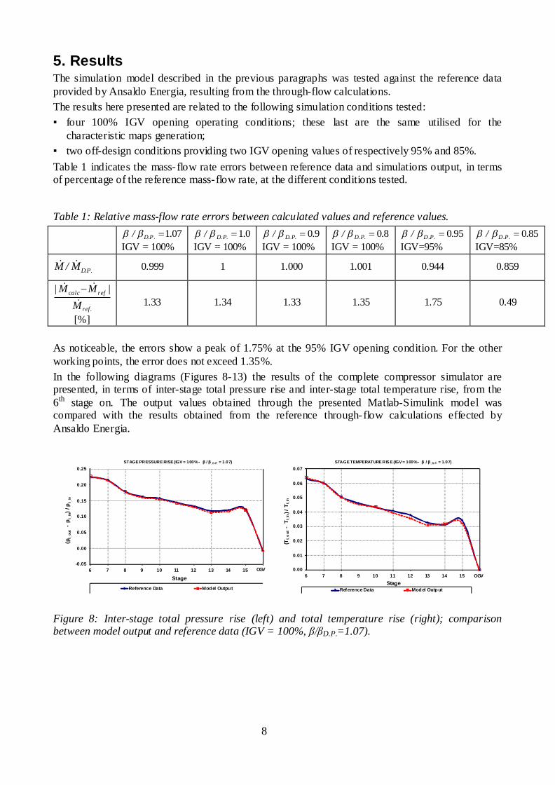
5. Results The simulation model described in the previous paragraphs was tested against the reference data provided by Ansaldo Energia, resulting from the through-flow calculations. The results here presented are related to the following simulation conditions tested: four 100% IGV opening operating conditions; these last are the same utilised for the

characteristic maps generation; two off-design conditions providing two IGV opening values of respectively 95% and 85%.

Table 1 indicates the mass-flow rate errors between reference data and simulations output, in terms of percentage of the reference mass-flow rate, at the different conditions tested.

Table 1: Relative mass-flow rate errors between calculated values and reference values.

071./ .P.D IGV = 100%

01./ .P.D IGV = 100%

90./ .P.D IGV = 100%

80./ .P.D IGV = 100%

950./ .P.D IGV=95%

850./ .P.D IGV=85%

.P.DM/M 0.999 1 1.000 1.001 0.944 0.859

.

||

ref

refcalc

MMM

[%]

1.33 1.34 1.33 1.35 1.75 0.49

As noticeable, the errors show a peak of 1.75% at the 95% IGV opening condition. For the other working points, the error does not exceed 1.35%. In the following diagrams (Figures 8-13) the results of the complete compressor simulator are presented, in terms of inter-stage total pressure rise and inter-stage total temperature rise, from the 6th stage on. The output values obtained through the presented Matlab-Simulink model was compared with the results obtained from the reference through-flow calculations effected by Ansaldo Energia.

-0.05

0.00

0.05

0.10

0.15

0.20

0.25

6 7 8 9 10 11 12 13 14 15 16

(pt_

out

-p t

_in)

/ p t

_in

Stage

STAGE PRESSURE RISE (IGV = 100% - / _D.P. = 1.07)

Reference Data Model Output

OGV 0.00

0.01

0.02

0.03

0.04

0.05

0.06

0.07

6 7 8 9 10 11 12 13 14 15 16

(Tt_

out

-

T t_i

n) /

Tt_

in

Stage

STAGE TEMPERATURE RIS E (IGV = 100% - / _D.P. = 1.07)


OGV

Figure 8: Inter-stage total pressure rise (left) and total temperature rise (right); comparison between model output and reference data (IGV = 100%, D.P.=1.07).

9

-0.05

0.00

0.05

0.10

0.15

0.20

0.25

6 7 8 9 10 11 12 13 14 15 16

(pt_

out

-p t

_in)

/ pt_

in

Stage

STAGE PRE SSURE RIS E (IGV = 100% - / _D.P. = 1)


OGV0.00

0.01

0.02

0.03

0.04

0.05

0.06

0.07

6 7 8 9 10 11 12 13 14 15 16

(Tt_

out

-T t

_in)

/ T t

_in

Stage

STAGE TEMPERATURE RISE (IGV = 100% - / _ D.P. = 1)


OGV

Figure 9: Inter-stage total pressure rise (left) and total temperature rise (right); comparison between model output and reference data (IGV = 100%, D.P.=1).

-0.05

0.00

0.05

0.10

0.15

0.20

0.25

6 7 8 9 10 11 12 13 14 15 16

(pt_

out

-p t

_in)

/ p t

_in

Stage

STAGE PRESSURE RISE (IGV = 100% - / _ D.P. = 0.90)


OGV

0.00

0.01

0.02

0.03

0.04

0.05

0.06

0.07

6 7 8 9 10 11 12 13 14 15 16

(Tt_

out

-T t

_in)

/ T t

_in

Stage



OGV


-0.05

0.00

0.05

0.10

0.15

0.20

0.25

6 7 8 9 10 11 12 13 14 15 16

(pt_

out

-p t

_in)

/ pt_

in

Stage

STAGE PRES SURE RISE (IGV = 100% - / _D.P. = 0.78)


OGV

0.00

0.01

0.02

0.03

0.04

0.05

0.06

0.07

6 7 8 9 10 11 12 13 14 15 16

(Tt_

out

-T t

_in)

/ T t

_in

Stage



OGV


10

-0.05

0.00

0.05

0.10

0.15

0.20

0.25

6 7 8 9 10 11 12 13 14 15 16

(pt_

out

-p t

_in)

/ p t

_in

Stage

STAGE P RESSURE RISE (IGV = 95% - / _D.P. = 0.94)


OGV0.00

0.01

0.02

0.03

0.04

0.05

0.06

0.07

6 7 8 9 10 11 12 13 14 15 16

(Tt_

out

-T t

_in)

/ T t

_in

Stage

STAGE TEMPERATURE RIS E (IGV = 95% - / _ D.P. = 0.94)


OGV


-0.05

0.00

0.05

0.10

0.15

0.20

0.25

6 7 8 9 10 11 12 13 14 15 16

(pt_

out

-p t

_in)

/ pt_

in

Stage

STAGE PRESSURE RIS E (IGV = 85% - / _D.P. = 0.83)


OGV

0.00

0.01

0.02

0.03

0.04

0.05

0.06

0.07

6 7 8 9 10 11 12 13 14 15 16

(Tt_

out

-T t

_in)

/ Tt_

in

Stage

STAGE TE MPERATURE RISE (IGV = 85% - / _ D.P. = 0.83)


OGV


Model outputs show a well acceptable agreement with the reference inter-stage total pressure and temperature rise data.

6. Conclusions A one-dimensional stage by stage model, integrated with a classical map-based single block model, was developed to predict the design and off-design performance of a multistage axial flow compressor. Being the first stages affected by transonic flow, not reproducible by the simple similitude theory based on i, i and i non-dimensional parameters not variable in function of Mach number, stages 1 to 5 were simulated by a map-based block. The remaining ten stages were simulated by the ordinary Stage Stacking method. The individual stage non-dimensional characteristics ( i=fi i) and i=gi i)) were estimated by means of an auxiliary stage by stage model, basing on inter-stage total pressure and temperature reference data calculated by a through-flow simulator. Moreover, according to Similitude Theory, the single stage characteristic maps were normalised by the Design Point values ( i,D.P., i,D.P. and

i,D.P.), obtaining two general stage maps valid for the whole machine.

11

As shown in the presented results, the model is able to reproduce with good precision the machine performance for a wide range of working conditions. The new stage by stage compressor model has been developed to replace the old single-block map-based one into the dynamic simulator of the Ansaldo AE94.3A gas turbine, enhancing its prediction capability; in particular, thanks to the model stage by stage structure, a better reproduction of the blade cooling system performances is possible, since the total pressure and total temperature values of the cooling air bleedings are correctly calculated. The next step to be done is the incorporation in the compressor model of the inter-stage volumes provided of continuity and energy equations in the time-varying form, making the simulator able to reproduce the machinery dynamic behaviour.

Appendix A The mathematical model utilised for the stage by stage simulator is based on the known Stage-Stacking technique, and has been developed in the Matlab-Simulink environment; its construction was effected following three steps: 1. introduction of the physical equations that rule the stacking of stages and OGV duct in the

simulation programme; 2. evaluation, for different machine working conditions, of the set of non-dimensional parameters

i, i and i for each stage i [11] [16]; 3. on the basis of the data collected in step 2), construction of the stage non-dimensional

characteristic curves i = i i) and i = i i) [18]. The non-dimensional parameters i, i and i utilised are defined in equations (1), (2) and (3). The parameters needed to apply the Stage-Stacking procedure are: total temperature and pressure at the compressor inlet station, shaft rotational speed, geometrical stage data (inlet flow passage areas

i and mean stage diameter), relative air humidity, mass flow rate and 10 stage characteristic curves i = i ( i) and i= i ( i), (i = 6,…,15) [8 ,13]. The evolving fluid was considered as a perfect

gas. Mass flow rate evolving in the compressor is calculated in the single block model (stages 1 to 5 + IGV, described in Paragraph 5), working with its typical performance maps [17]; the calculated flow rate value deviates from the reference data of no more than 1,75%, as indicated in Table 1, in the totality of the working conditions investigated. Figure 14 shows the structure of one stage block; the sequence of steps by which the input signals are elaborated to calculate the output values [12] is described in the following.

Figure 14: Scheme of one stage.

1. The “Density” block calculates the flow inlet static density from the inlet total pressure and temperature and the absolute air humidity exploiting, in sequence, the general formulas:

12

12

21

1kk

t

Mk

pp

(4)

2

21

1 Mk

TT t

(5)

RTp

(6)

2. In the “Continuity Equation” block, known flow passage area and mass flow rate, it is possible to obtain axial velocity ca_i and derive the flow-rate coefficient i, dividing ca_i by the mid-span rotor velocity, ui. This operation takes place into the block indicated with the label “ ”.

3. Pressure coefficient i is calculated in the block “Map ”, containing the i= i i) characteristic curve for the ith stage.

4. Pressure coefficient definition permits to find the stage pressure ratio, through Equation 7:

1

1_

2

1_

_ 1kk

itp

ii

it

iti Tc

upp

(7)

From this relation, it is immediate to find stage outlet total pressure, pt_i. 5. Stage efficiency i is calculated in the block “Map ”, containing i = i ( i) stage characteristic

curve. 6. Once known the efficiency, it is possible to obtain the outlet total temperature by means of

Equation 8:

pi

iiitit c

uTT2

1__

(8)

7. Stage outlet total pressure and temperature represent the inlet values for the following stage: in this way, proceeding stage by stage, it is possible to calculate the compressor outlet conditions.

Acknowledgements The Authors wish to thanks Franco Rocca, Raffaele Traverso and Daniela Marino of Ansaldo Energia for the reference data of the AE94.3A gas turbine, and for the permission of their publishing in this paper.

Nomenclature ca axial flow velocity, m s-1 F, Ggeneric function H enthalpy, J kg-1 cp specific heat capacity at constant pressure, J kg-1 K-1 IGV inlet guide vanes k specific heat ratio, -

mass-flow rate, kg s-1

Ma Mach number,-

13

n shaft rotational speed, rev s-1 p pressure, Pa R individual gas constant, J kg-1 K-1

T temperature, K u rotor speed at the mean diameter, m s-1

Greek symbols pressure ratio, - efficiency, - mass-flow coefficient, - pressure rise coefficient, - flow passage area, m2

Subscripts D.P. design point i related to the i th stage red reduced ref reference r real s isentropic t total (stagnation)

References [1] Aretakis N., Roumeliotis L., Mathioudakis K., “Performance Model Zooming for in-depth

Component Fault Diagnosis”, 2011, ASME J. of Engineering for Gas Turbines and Power 133 (3).

[2] Morini M., Pinelli M., Spina P.R., Venturini M., “Influence of blade deterioration on compressor and turbine performance”, 2010, ASME J. of Engineering for Gas Turbines and Power, 132 (3).

[3] Reza Hosseini S.H., Khaledi H., Soltani M.R., “New Model Based Gas Turbine Fault Diagnostics Using 1D Engine Model and Nonlinear Identification Algorithms” 2009, Proceedings of the ASME Turbo Expo, 1, pp. 575-585.

[4] White N.M., Tourlidakis A., Elder R.L., “Axial compressor performance modelling with a quasi-one-dimensional approach”, 2002, Proc Instn Mech Engrs, Part A: Journal of Power and Energy, 216 (2), pp. 181-193.

[5] Schulte H., Schmidt K.J., Weckend A., Staudacher S., “Multi Stage Compressor Model for Transient Performance Simulations”, 2008, Proceedings of the ASME Turbo Expo, 1, pp. 185-195.

[6] Saravanamuttoo H.I.H., “Component performance requirements”, 1992, Nato, Agard-LS-183, pp. 1-4.

[7] Horlock J. H., “A Rapid Method for Calculating the “Off-Design” Performance of Compressors and Turbines”, 1958, The Aeronautical Quarterly, pp. 346-360.

[8] Tsalavoutas A., Stamatis A., Mathioudakis K., “Derivation of Compressor Stage Characteristics for Accurate Overall Performance Map Prediction”, 1994, Proceedings of the International Gas Turbine and Aeroengine Congress in Exposition, Hague (Netherlands), 13-16 June.

[9] Robbins H., Dugan J.F., “Prediction of Off-Design Performance of Multistage Compressors”, 1965, Aerodynamic Design of Axial-Flow Compressors, NASA SP-36, pp. 302-304.

14

[10] Benser W.A., “Compressor Operation with One or More Blade Rows Stalled”, 1965, Aerodynamic Design of Axial-Flow Compressors, NASA SP-36, pp. 341-364.

[11] Howell A.R. and Bonham R.P., “Overall and stage characteristics of axial flow compressors”, 1950, Institutions of Mechanical Engineering, 163, pp. 235-248.

[12] Mellor G.L., Root T., “Generalized Multistage Axial Compressor Characteristics”, 1961, Transactions of the ASME, Series D.

[13] Song T.W., Kim T.S., Kim J.H., Ro S.T., “Performance Prediction of Axial Flow Compressors Using Stage Characteristics and Simultaneous Calculation of Interstage Parameters”, 2001, Proc Instn Mech Engrs, Part A: Journal of Power and Energy, 215, pp 89-98.

[14] Aker, G. F., and Saravanamuttoo, H. I. H., 1989, "Predicting Gas Turbine Performance Degradation Due to Compressor Fouling Using Computer Simulation Techniques," ASME J. of Engineering for Gas Turbines and Power, 111 , pp. 343-350.

[15] Muir, D. E., Saravanamuttoo, H. I. H., and Marshall, D. J., 1989, "Health Monitoring of Variable Geometry Gas Turbines for the Canadian Navy, " ASME J. of Engineering for Gas Turbines and Power, 111, pp. 244-250.

[16] Ma W., Liu Y., Su M., Yu N., “Multi-stage axial flow compressors characteristics estimation based on system identification”, 2007, Energy Conversion and Management, 149 (2), pp. 143-150.

[17] Crosa G., Pittaluga F., Trucco A., Beltrami F., Torelli A., Traverso F., “Heavy Duty Gas Turbine Plant Aerothermodynamic Simulation Using Simulink”, 1998, ASME J. of Engineering for Gas Turbines and Power, 120 pp.550-556.

[18] A.R. Howell and W.J. Calvert, “A New Stage Stacking Technique for Axial-Flow Compressor Performance Prediction” , 1978, Journal of Engineering for Power, Transactions of the ASME, 100, pp. 698-703.



15

A flexible and simple device for in-cylinder flow measurements: experimental and numerical

validation

Andrea Dai Zottia, Massimo Masib, Marco Antonelloc a Ebara Pumps Europe S.p.A., R&D Dept., Brendola-Vicenza, Italy, [email protected]

b University of Padova, Dept. of Management and Engineering, Vicenza, Italy, [email protected] c University of Padova, Padova, Italy, [email protected]

Abstract: Deep knowledge of intake process aerodynamics is fundamental to development and optimisation of modern internal combustion engines. In particular, the intake port flow strongly affects both volumetric efficiency, i.e. power output, and in-cylinder charge motion which influences combustion behaviour and pollutants formation. The paper presents an experimental and numerical study of intake airflow through ports and cylinder in a four-valves pent-roof motorbike high-speed engine. A very simple mechanical device specifically designed for quick and low-cost measures of swirl and tumble motions in steady-state discharge flow coefficient test rigs was developed and checked on two twin-cylinder stock production heads featuring intake ports design typical of modern motorbike high speed SI engines. Simultaneous measures of discharge flow and tumble coefficients proved the limited error due to device insertion. A detailed CFD model of cylinder, intake ports, and manifolds within the engine head was build and experimentally validated by discharge-flow coefficient measurements performed at different valve li ft. The sensitivity to grid refinement and the performance of a realizable k - and a modified k - turbulence models is investigated. The numerical model is used to evaluate the reliability of tumble measurements. The correlation between experimental data and the whole CFD velocity field within cylinder volume is very good proving that the device appears well -suited for rapid and reliable analysis of aerodynamic bulk performance of engine heads.

Keywords: Tumble measure, Tumble and discharge flow coefficients, in-cylinder flow CFD calculation, grid and turbulence model for intake ports computations.

1 Introduction Design of intake ports for high speed engines equipping stock production motorbikes results from an aerodynamic trade-off between two counteracting requirements: high volumetric efficiency and intense motion of fresh charge trapped within cylinders. It is well-known (see e.g. [1-6]) that processes like air- fuel mixing, start and development of combustion, cylinder wall heat transfer and pollutant formation are greatly influenced by squish, swirl and tumble motions. These two latter can be experimentally studied by means of both mechanical and optical instrumentation. Many types of paddle wheel or honeycomb flow straightener used to sense angular velocity or momentum, respectively, belong to the first category of instrumentation. Angular speed of the wheel or torque T exerted by the vortex flow on the impulse-meter within an appropriately located equivalent of the cylinder, are measured during traditional steady-state tests at discharge flow test rigs. Thus, meaningful similarity parameters such as swirl or tumble coefficients and numbers are defined as in [7, 8]. The main difference in the experimental measurements of swirl and tumble motions is the location of the sensor. In fact, the quite simple location of the swirl-meter directly within the equivalent of the cylinder is usually substituted by the more complex apparatus constituted by a cylindrical reversed T-junction, required to symmetrically split the tumbling flow towards the two openings each one provided of an impulse-meter or a paddle wheel.

16

On the other hand, the up-to-date optical and electronic instrumentation allows very detailed measurements of the local vector field within the cylinder both under steady-state ([5, 8-10]) and unsteady test rig operations (see e.g. [5, 11-14]). Other parameters of swirl and tumble are more properly suited to this type of instrumentation [2-4, 14, 16]. Many researchers studied the correlations between traditional test rig data of discharge flow and the newer optical measurement systems. Omori et al. [6] investigated the airflow vector field featured by various intake runner layouts in the region upstream and around the valve, and within the cylinder. Tumble index calculated from LDV data, collected for engine heads featuring different runner design (traditional, straight, straight with shielded valves), was compared to tumble coefficient, derived by traditional measurements performed on discharge-flow test rig for the same engine heads. In this work an excellent correlation between experimental tumble parameters is assessed. Kim et al. [18], focusing on the correlation between tumble parameters calculated from data obtained by PIV, PTV, and traditional impulse-meter, corroborated the experimental findings of Omori et al. [6]. Algieri et al. [19] verified good reliability of swirl measurements obtained by impulse sensor extrapolated from optical systems data. In [8, 10] Kang and Reitz studied swirl intensity within a medium-bore compression ignition engine. Once again, they proved the good agreement between optical instrumentation and torque sensor data. The flow field of port-valve-cylinder systems is widely studied from many years also through CFD techniques, which give very detailed predictions that can be useful to better explain experimental evidences, and to aid the designer work. Pioneering CFD researches on engines modelled the flow field close to and downstream of intake valves. In 1985 Gosman [20] obtained qualitative good agreement between calculated and measured flow fields and, in a succeeding work [21], proved that the discharge-flow coefficient for a simplified valve port can be numerically predicted with acceptable accuracy. Brandstaatter et al. [12] focused their effort on in-cylinder flow performing 3D CFD simulation of cylinder volume starting from results of 1D gas-dynamic code and velocity measure at the curtain valve section. They succeeded on capturing the vortex flow in the recirculating zone between valve and cylinder liner wall, and the swirl motion structure on various cylinder heights. However, they highlight limitations related to standard k- turbulence model. Among other works Dent and Chen [22] accurately predicted valve lifts for which flow separation from valve lip and from valve seat occur. Steady-state calculations capable to correctly estimate the discharge-flow coefficient and satisfactorily correlate numerical and experimental swirl indices were performed by Befrui [23], Godrie and Zellat [16]. In 2000 Kang and Reitz [8] compared their experiments with previous CFD computations performed with KIVA 3V code in [24], and showed the calculations under-estimation in both swirl and tumble charge motion. In the same period Hong and Tarng [9], using KIVA 3 and optical LDV measurements, find appreciable correlation between rather basic calculations and experimental data for tumble ratios. However, both their local and overall in-cylinder flow calculations with standard k- turbulence model, notably over-predict tumble intensity. Ramajo and Nigro [25] after the validation of their numerical model by comparison of discharge-flow coefficient, tumble, and swirl indices with corresponding parameter value measured during steady-state flow tests, performed time-dependent calculations for the whole engine cycle. They proved that tumble moment versus valve lift shows the same features during steady and unsteady operation. The paper presents an experimental and numerical study of intake airflow through ports and cylinder in a four-valves pent-roof motorbike high-speed engine. The main aim of the work is to verify the reliability of a very simple mechanical device specifically designed for quick and low-cost measurements of swirl and tumble motions in steady-state discharge-flow coefficient test rigs. A “spherical” paddle wheel, which has to be located in the cylinder downstream the head under analysis and does not require special T-junction ducts to sense tumble motion, was used to experimentally test two twin-cylinder stock production heads featuring different intake port design, which are typical of modern motorbike high speed engines. The more traditional head, featuring low tumble intensity, is then selected to check the designed device in the less favourable condition.

17

Since CFD results are used to better understand swirl and tumble data, numerical predictions require an experimental validation by different measured flow parameters. For this purpose, since the test rig is a traditional steady-state flow bench, the choice of discharge-flow coefficient is straightforward. Concerning numerical simulations, the selection of an appropriate RANS turbulence model is an important issue. Indeed, in-cylinder flows are mainly characterised by jet interactions with walls, recirculation regions, vortex flow, and three-dimensional effects. Reynolds-stress transport models (RSTM) are able to describe all the above-mentioned features but they suffer from a great computational cost [26], and from a strongly simplified near-wall modelling [27]. For these reasons, in the simulation of industrial complex flows, the class of nonlinear eddy viscosity models (NLEVM), based on k and transport equations, and the class of k- models are most frequently employed. Concerning in-cylinder flows, numerical studies confirmed that Wilcox k- model and NLEVMs are suitable to reproduce the flow field inside the combustion chamber and the quantification of the overall angular momentum with respect to the cylinder axis (see e.g. [34, 35]). For all the reasons the present numerical study has been carried out with the realizable model of Shih et al. [36], which is one of the most successful NLEVM, and with the modified k- model of Wilcox [31]. Finally the validated CFD model is used to evaluate the reliability of the tumble measurements looking at the correlation between numerical and experimental tumble indices.

2 Experimental facility The test rig used for present experiments is a traditional discharge-flow test rig, derived from an A-type industrial fan test rig built according to the UNI 10531 Italian Standard [37], which is equivalent to the ISO 5801 Standard. The main scheme of the original test rig is described in details by Martegani et al. [38]. The original facility has been modified in a previous work [39] by substituting the auxiliary fan with a variable speed fan that generates a negative relative constant pressure inside the plenum chamber faced to the engine head to be analysed. The mass flow across valve port is derived from conventional measurements: dry and wet-bulb ambient temperature and the temperature inside the plenum chamber are measured using mercury thermometers; barometric pressure is measured using a mercury barometer, whereas a water manometer is used to measure the pressure in the plenum chamber. Finally, a differential water manometer measures differential pressure of orifice plate, which is needed for flow rate determination. The accuracy estimated by the Kline-McClintock criterion is about 1% for all the presented discharge coefficient measurements.

2.1 Swirl and tumble meter Classically adopted mechanical devices to measure in-cylinder motion are usually paddle wheels or honeycomb flow straightener impulse-meters. They provide in-cylinder flow parameters such as the following swirl or tumble coefficient and number (see e.g.[7, 8]):

isvD=C

isDvmT=N 8

(1)

Where vis is the isentropic velocity due to the actual pressure drop across the inlet ports, m is the actual mass-flow rate, and D is the cylinder bore.

18

The well-established set-up for these devices usually is not conceived to allow an easy switch from swirl to tumble analysis layout. The device used to measure charge motion intensities within the cylinder has been designed to cope with the following requirements: suitability for both swirl and tumble tests to simplify the test rig instrumentation required for

basic measurements; low flow field modification to allow simultaneous analysis of charge motion and discharge-flow

performance, if desired; easy manufacturing to allow in-house building without sophisticated machining and remarkable

cost of sensors; quickness and simplicity of use with usual steady-state discharge flow test rigs to assure rapid

and repeatable measurements with minimum risk of human error. Figure 1 shows exploded views of the main parts arranged within the core of the mechanical assembly for charge motion measurement.

a) b)

Fig. 1. Exploded views of the mechanical assembly including the charge motion transducer: a) swirl measurement layout, b) tumble measurement layout.

To deal with first item the charge motion transducer has spherical shape so that it can be inserted within a cylinder of actual engine bore, which is flanked downstream the assembly of runners, valves, and combustion chamber under analysis (i.e. the proper engine head section). Depending on the layout, the transducer can spin around an axis overlaid or perpendicular to cylinder axis (see figure 1). Since impulse sensors act like walls counteracting flow motion and greatly affect discharge flow coefficient measurement, paddle wheel is mandatory to try fulfilment of second requirement. Moreover, the circular plates arranged in the wheel has been machined to be lens shaped in order to reduce flow blockage, device inertia, and mechanical friction due to weight action on wheel pivotal bearings. The third item can be fulfilled using cheap metallic duct sections for the equivalent of the cylinder (alloy if the overall assembly weight is a problem, or plexiglass if money saving is not so strict) and light sheets as prime matter to be lens shaped machined, which is actually the sole process requiring some carefulness. Being the paddle wheel steel made, a simple and inexpensive proximity sensor, which counts blade passing, can be used.

19

a) b)

Fig. 2. Complete assembly of charge motion mechanical meter: a) swirl measurement layout mounted on test chamber of the used discharge-flow coefficient rig, b) tumble measurement layout mounted on one of the two actual engine heads analysed.

Finally, the last needing can be well satisfied. In fact Figure 2a) shows that effort to set-up the discharge-flow test rig is very slightly affected by the simple insertion at openings of the main cylindrical duct section of two annular slices, required to pivot the paddle wheel for swirl measurements. Similarly, the easy repositioning of the two low friction plug bearings for tumble measurements, which are well visible in Figure 1b), ends in the assembly illustrated in Figure 2b). The specific equipment used for present measurements includes an electric power unit, which can be both voltage and current regulated, and the “virtual oscilloscope” library tool provided with Labview®, which easily counts the blade passing close to the proximity sensor. The main features of this proximity sensor are reported in Table 1. Since the paddle wheel counts 4 blades, the resolution of present instrumentation is a quarter of the last paddle wheel revolution occurred during the measurement time interval. As a consequence, the higher the charge motion intensity and the time interval the higher the overall accuracy. Following this reasoning the accuracy error is negligible. The main cylinder section features a transparent window in the paddle wheel location zone, which is clearly visible in both Figure 1 and Figure 2. This window provides the immediate feeling on effectiveness and proper assembly of instrumentation.

Table 1. Main features of proximity sensor equipping charge motion meter assembly Manufacturer OMRON Model EA-S08LS01-WP-B1 Sensing distance 1.5 mm (iron-magnetic materials) Maximum frequency 2000 Hz Voltage input 10-32 V (DC) Current output (max) 200 mA (32 VDC) Output type PNP with signal occurring for distance sensing distance

2.2 Ports, valves and combustion chamber assemblies The main characteristics of the two twin-cylinder stock production heads used to check the instrumentation presented in the previous section, are reported in Table 2. These heads feature different intake ports design typical of modern motorbike high speed engines. Both of them are swirl- free, as usual for high speed SI engines. Nevertheless Aprilia’s head shows the classical layout for high volumetric efficiency featuring curved intake runners and reduced angle between intake and exhaust. On the other hand, Ducati’s head favours rapid combustion thanks to in-cylinder tumble induced by straight intake runners.

20

Table 2 Main features of production engine heads under analysis. Manufacturer Aprilia S.p.A. Ducati S.p.A. Motorbike model RSV 1000 999 Engine architecture Twin-cylinder V 60° liquid cooled Twin-cylinder V 90° liquid cooled Distribution 4 valve DOHC 4 valve DOHC Combustion camber layout pent-roof pent-roof Stroke/Bore 67.5 mm / 97 mm 63.5 mm / 100 mm Compression ratio 11.8 11.4 Intake valve diameter dv 37.95 mm 40 mm Valve seat diameter ds 33.6 mm 36.95 mm Valve lift (measured) 11.78 mm 11.78 mm Sketch of intake runners, intake ports, valves and combustion chamber assembly

3 Tumble meter validation Imposing no- lift to one of the two intake valves to artificially induce in-cylinder swirling flow, a preliminary check on capability of the assembly to measure swirl motion has been performed, through discharge-flow coefficient tests. However, the device validation is focused on tumble motion measurements, being this charge motion the most critical to be characterised with an unique tumble coefficient. In fact, it is well-known that tumble vortex can present different shape, eccentricity, and vertical position of its axis depending to valve lift [13] also in steady-state tests. Moreover the effectiveness of such a device to give reliable data about in-cylinder tumble motion need to be verified just because of the original layout, which does not include nor actual piston crown nor any other piston dummy always provided in steady-flow rigs tumble meters. Actually, it is a matter of fact that in a real engine the presence of the piston surface plays a relevant role in the onset of tumble vortex. On the other hand, just due to the presence of the piston surface, every pent-roof four-valve head in actual engines features a certain degree of tumble motion. Following the results of [6] what is hypothesised as the base for the design of present device is that not the piston surface, but the intake ports design and their interaction with cylinder liner are the more relevant items in the establishing of different tumble intensity level. Thus, the validation procedure develops as follows:

1) comparison between tumble coefficient measured for the two heads in order to verify the sensitivity to different head design;

2) comparison of these coefficients with published data typical of engine heads featuring similar layout;

3) comparison between discharge-flow coefficient measurements performed with and without paddle wheel, in order to quantify the blockage effect of the rotating device and, consequently, the experimental error related to simultaneous discharge-flow and tumble coefficient measurements.

3.1 Tumble coefficients The intensity of charge motion is measured at different valves lift for both the engine head under analysis. Starting from zero-lift condition, which is needed to verify the negative pressure-proof of the test chamber and zero-offset condition of the whole instrumentation, the lift is increased by 0.5 mm steps until 1.5 mm lift. Higher lift values are tested by 1 mm steps until 11.25 mm for both the heads. Five non-sequential measurement repetitions are made for each valve lift conditions featuring paddle wheel rotation (i.e. appreciable tumble), in order to reduce random accuracy error.

21

The arithmetic mean value of tumble coefficient defined according to (1a) is assumed as experimental tumble data. Figure 3 shows the tumble coefficient values against valves lift for both the heads under analysis. Error bars refers to a confidence of 99.5% for experimental data according to Student distribution. It appears that present instrumentation is capable to sense the difference in tumble intensity existing between two runner-valve-combustion chamber assemblies featuring different conceptual design. In fact, the behaviour of tumble coefficient against lift is in line with the figures provided by Omori et al. [6] discussed in the next section. As a general comment Aprilia head, not specifically conceived to originate high tumble, shows a quite regular increase in tumble intensity which, however, reaches values for high valve lift well above the corresponding ones featured by Ducati. This latter, designed for a more pronounced tumble motion, shows lower intensities than Aprilia until the proper onset of tumble vortex. Other tests, not presented here, were performed for different pressure ratio values across intake valve measurements. However, they revealed to be less sensitive to Reynolds and Mach numbers than discharge flow coefficient measurements. Thus, this tumble coefficient measurement defines a cinematic property of in-cylinder flow field, which is to be considered as a similarity parameter, at least in the limits stated for discharge flow coefficients.

-0 .10

0 .00

0 .10

0 .20

0 .30

0 .40

0 .50

0 1 2 3 4 5 6 7 8 9 10 11 12

valve lift [mm]

tum

ble

coef

ficie

nt C

t RSV1000999

Fig. 3. Tumble coefficient against valve lift for Aprilia RSV1000 (blue) and Ducati 999 (red) heads.

3.2 Comparison with other published data In order to check if present device may be used to acquire something more than the hierarchic rank of tumble flow onset capability, due to different intake port design, a comparison with some published data [6, 43, 44] measured by tumble meter devices of consolidated use is presented. Although the head designs are not radically different to the present ones, a complete comparison with previously referenced data is almost impossible, because of the uncertainty both on detailed features of engine heads and on values used by some of those authors to provide non-dimensional data. Thus, Figure 4 compares to present measurements the referenced data some of which were scaled by an arbitrary factor reported in figure legend. First considering the classical reference (1991) of Omori et al. [6] which offers measurements collected from a series of intake ports of different conceptual design, it appears that the quite low-tumble design of Aprilia head shows tumble coefficient figure in line with the low-tumble head design F of the cited reference [6], since the higher tumble design of Ducati head shows figure more similar to the head design E of the same reference [6]. The comparison appears to be satisfactory enough only for medium-to-high valve lifts. More recent (2000) measurements of tumble coefficient on a pent-roof four-valve car engine

22

head were presented by Yun and Lee [15]. They used the classical honeycomb wheels at the end of a T-junction duct. Green curve of Fig.4 refers to these data without any rescaling. Slope of the curve is in the middle of the present measurements and the agreement appears acceptable also for low valve lift values. Finally, a very recent work (2011) of Moore et al. [17] is considered. These authors show, among other interesting data, the tumble index map measured at the flow bench in a SI direct injection turbocharged engine head where many combinations of intake valves lift are tested. To make possible a comparison with the tumble index used by those the rescale by the arbitrary factor 3 is performed to originate orange curve in Fig.4. This data trend, except for the very low valve lift values, is in very good agreement with present measurements on Ducati 999 head. Note that Moore and co-authors stated that the port design of the engine head used in their work was conceived for high tumble intensity making possible to argue an head design more similar to the Ducati one than the Aprilia one. At least within the limits of this incomplete comparison, present device appears to be capable to capture the main tumble features of the bulk in-cylinder flow in the medium-to-high valve lift ranges, which are the most relevant in the onset of tumble intensity level at the compression top dead centre in actual engines, as assessed by LDV measurements on the single-cylinder optical engine arrangement performed by [6]. However, it is worth noting that present measurements lack of the abrupt rise of the tumble torque typical of very high tumble intensity head designs. This could be due to the design of the heads used for present work. On the other hand the possibility that the absence of a piston crown dummy in present device affects especially low lift valve measurements has to be accounted for.

0,00

0,10

0,20

0,30

0,40

0,50

0,60

0,70

0 0,04 0,08 0,12 0,16 0,2 0,24 0,28 0,32non-dimensional valve lift h/ds

tum

ble

coef

ficie

nt C

t

Ct RSV1000 Ct 999

Ti/3 ref. [17] (Fig.1 a) Nt ref. [15] (Fig.2)

Rt/3 ref. [6] (Fig.12 F) Tr/3 ref. [6] (Fig.12 E)

Fig.4. Tumble coefficient against non-dimensional valve lift for Aprilia RSV1000 (blue), Ducati 999 (red), ref. [6] (cyan and black) ref. [15] (green) and ref [17] (orange) heads.

23

3.3 Discharge-flow coefficients Overall aerodynamic performance of the engine heads are measured through the well-known discharge-flow coefficient

i

r

mm=C 3),

where rm and im are actual and ideal constant-entropy one-dimensional steady-state mass flow rate across the conventional throttle section of the port, which is calculated for the actual valves pressure drop. As stated in section 2 the overall mass flow accuracy estimated for maximum lift is about 1%. In order to quickly evaluate aerodynamic performance at high and low valve lift values, the following well-known reference sections are assumed, respectively: valves head area, which is lift independent and gives the non-dimensional coefficient Cd; curtain area, which is lift dependent and gives non-dimensional coefficient Cf [7].

Figure 5 shows the steady-state direct discharge-flow coefficients measured for Aprilia and Ducati heads, for lift values ranging from 0 mm to 7 mm with 0.5 mm lift step, and with 1 mm lift step until maximum valve opening is reached.

0.0

0.1

0.2

0.3

0.4

0.5

0.6

0.7

0.8

0 1 2 3 4 5 6 7 8 9 10 11 12valve lift [mm]

Cd

0.0

0.1

0.2

0.3

0.4

0.5

0.6

0.7

0.8

Cf

Cf 999Cf RSV1000

Cd 999

Cd RSV1000

Fig. 5. Discharge-flow coefficients against valve lift for Aprilia RSV1000 (Cd continuous blue; Cf dotted blue) and Ducati 999 (Cd continuous red; Cf dotted red) heads.

Finally, to quantify the effect of flow blockage and aerodynamic obstruction due to the simultaneous measure of discharge-flow and tumble coefficients, Figure 6 compares the solid lines referring to the discharge-flow coefficients Cd already shown in Figure 5 with the same coefficients measured during the tumble flow tests discussed in the previous section.

24

0.00

0.10

0.20

0.30

0.40

0.50

0.60

0 1 2 3 4 5 6 7 8 9 10 11 12

valve lift [mm]

disc

harg

e-flo

w c

oeffi

cien

t Cd

RSV1000RSV1000 (no wheel)999999 (no wheel)

Fig. 6. Discharge-flow coefficients Cd against valve lift for Aprilia RSV1000 (blue) and Ducati 999 (red) heads, measured with and without paddle wheel.

Maximum error on discharge-flow measurements due to aerodynamic interference of paddle wheel results 2.3% for Aprilia head and 0.7% for Ducati head at maximum valve lift (11.25 mm). This evidence demonstrates the limited sensitivity of steady-state in-cylinder flow field to present instrumentation. Moreover, the instrumentation appears to reduce its interference on in-cylinder flow field as more as higher the charge motion intensity is, revealing to be well-suited for quick in-cylinder charge motion analysis, especially in engine heads designed to maximise the charge motion itself. Indeed, it is quite secure the occurrence of a small blockage effect on the valve flow originated by the paddle wheel insertion, which penalises the higher discharge flow coefficient of Aprilia at higher lift values. Less clear is the improvement of discharge flow coefficient featured by test performed on Ducati head when the paddle wheel is inserted. A possible explanation of this occurrence is that the paddle wheel strengthens the rigid body motion character of bulk flow. This reduces near-wall recirculation close to the intake runner exit on the opposite side of the exhaust. Thus, viscous losses and vortices blockage are smoothed. However, detailed information about actual flow motion within the cylinder enclosing paddle wheel must be acquired to support this reasoning.

4 Numerical analysis The limited influence of paddle wheel on in-cylinder flow field assessed by experiments suggests comparing the measured tumble intensity with the detailed charge motion description achievable from a validated CFD model of the fluid domain enclosing the intake manifold, valves and cylinder system. This comparison appears particularly useful to reduce the uncertainty related to the reliability of tumble measurements. This is not a style exercise for all those researchers and applied engineers who can not dispose of very sophisticated and expensive optical instrumentation. Indeed, numerical results can be used like optical measurements to evaluate the correlation existing between motion intensity of overall charge, measured by mechanical instrumentation, and velocity fields. Moreover, CFD data give whole cylinder volume velocity field and, thanks to in-cylinder integration, allow proper comparison with mechanical charge motion measurements. This comparison can be more effective than that between mechanical and optical measurements collected within a very limited number of plane sections. The more traditional head design, i.e. Aprilia RSV1000, is selected for the numerical analysis. The selection of a low tumble intensity configuration is aimed at checking the designed mechanical device in the less favourable condition.

25

4.1 Computational domain The physical domain, which was meshed to be numerically analysed, has been obtained by use of a reverse engineering technique. The manifolds, valves and combustion chamber geometry have been acquired by applying a laser scanning technique to a rubber ‘core’ obtained by filling the empty space within the ports and cylinder volumes (see left side of Figure 7). Surface data have then been handled with the Rapidform® 3D Scanning Software, before CAD surfaces reconstruction and addition of inlet and outlet plenums have been made as showed in right side of Figure 6. The detail of the whole reverse engineering work is reported in [40]. Summarising, the whole geometrical domain used for CFD analysis encloses an hemisphere used as inlet plenum (similarly to [41]), the bell-mouth duct before the intake runners, the air volume surrounding intake valves and pent-roof combustion chamber, the cylinder before experimental test rig plenum, and its CFD equivalent modelled by another hemisphere. The domain is almost symmetrical and this could advantage numerical calculation. However, the entire domain is discretised to account for un-symmetries due to casting and for the spark plug region within the dome of the combustion chamber, the axis of which intersects but does not lie in the mean cylinder plane.

Fig. 7. Reverse engineering of Aprilia RSV1000 cylinder geometry: “rubber” cores of combustion chamber and manifolds (upper left); intake system assembly to be 3D scanned (lower left); reconstructed CAD surface of the whole intake system CFD domain (right).

4.2 CFD model The steady-state RANS equations for turbulent incompressible and isothermal airflow are solved by commercial finite volume code Star CCM+® version 6.0.009 of CD-Adapco. These flow hypotheses are justified by the low pressure ratios involved in the experimental tests which, however, are not considered to be inadequate for intake valves within the limits of steady-state flow bench data. As mentioned in section 1, the complexity of in-cylinder flows requires a careful selection of the turbulence model to be used. From a theoretical point of view, Reynolds-stress transport models (RSTM) are able to describe all complex flow effects. However, they suffer from two main drawbacks: the computational effort is much larger than that of two equation models [26]; strongly simplified near-wall models must be introduced to systematically integrate transport equations in complex geometries [27]. As a result, in many cases where near-wall effects are relevant RSTM give similar or even worst predictions compared to those of two equation models [26, 28, 29]. For these reasons, in the simulation of industrial complex flows, the class of nonlinear eddy viscosity models (NLEVM), based on k and transport equations, and the class of k- models are most frequently employed. The first group, which also embodied the explicit algebraic Reynolds stress

26

models (EARSM), has the advantage of retaining to some degree the Reynolds stress anisotropy effects associated with a full differential closure [30]; while the second group, nevertheless the simpler representation of the stress tensor, gives rather good prediction for many flows with strong adverse pressure gradient and recirculations, and three-dimensional jets [26, 28, 29, 31] as well. This is due to the fact that these models describe quite well both the near-wall effects and the mechanisms of production and dissipation of the turbulent quantities. Wallin and Johansson [32] developed an EARSM based on k and equations that, however, has no met with much success in the simulation of engineering flows. One of the reasons is the too large value of turbulence dissipation predicted in some situations, which prevent to improve the results of the simpler k- model [33]. According to the above considerations, some numerical studies of in-cylinder flows confirmed that Wilcox k- model and NLEVMs improve the reproduction of the flow field inside the combustion chamber and the quantification of the overall angular momentum with respect to the cylinder axis (see e.g. [34, 35]). Thus, following these works, the present numerical study has been carried out with the realizable model of Shih et al. [36], which is one of the most successful NLEVM, and with the modified k- model of Wilcox [31]. The polyhedral grid capability is preferred to the more classical hexahedral trimmed grid approach to speed up mesh generation process, to minimise grid clustering in regions far from valves, to obtain high cell regularity also in proximity of surfaces of complex shape, to keep low advection term spreading and, finally, to take advantage of polyhedral cells to more accurately capture vortex flows. Near wall prism sub- layer is generated for all the solid surfaces. Dimension and number of layers as well as clustering and number of core cells are discussed in the following. Figure 8 shows the computational domain and particulars of the grid selected for 7 mm valve lift, after the grid sensitivity analysis. A pressure drop of 1500 Pa (derived by experimental data) is imposed between the two hemispherical openings of the simulation domain, shown in left side of Figure 8. The inflow turbulence intensity and length scale are 1.5% and 40 mm, respectively. The solid walls are modelled with the adiabatic no-slip condition, and a surface roughness ranging from 0.1 mm to 0.25 mm is imposed from upstream valve seats to valve guides zone. In fact, the intake valve manifold surface of the engine head is cast without finish, and the measured wall roughness for the previously mentioned zones is reported in Tab. 3. Numerical simulations are carried out using the realizable eddy viscosity model of Shih et al [36] and the k- model of Wilcox [31]. In the first model modifications of both the eddy viscosity expression and the transport equation for the dissipation rate are introduced. The eddy viscosity formulation ensures realizability through an expression that is nonlinear in mean strain rate components. The transport equation for is based on the dynamic equation for fluctuating vorticity. In the modified model of Wilcox the dissipation terms of both k and equations are modified to improve the predictions for free shear flows, giving boundary layer results equal to the original model. These models are selected, among most used two-equation models, because they give good descriptions of jet flows, expansions and recirculations [26, 28, 29, 31, 35], and the computational effort is moderately greater than that of the standard k- model.

27

Fig. 8. CFD model for steady-state flow analysis of Aprilia RSV1000 intake valves and cylinder: computational domain (left); volume mesh section lying on valve axis and parallel to cylinder mean plane (centre); valve zone grid (upper right); near-wall sub-layer near the curtain area (lower right)half-valve half-manifold plane of the main domain region used to model.

Wolfstein two-layer approach [42] is coupled with the realizable k- for near-wall calculation being wall-y+ values always lower than 30 (see following section). Second order upwind scheme is adopted to solve the steady-state RANS equations by means of a segregated SIMPLE-like algorithm. Calculations are considered to be converged when normalised residuals of conservation equations are below 1.5 E-5 and the mass flow rate is constant.

Table 3 Intake manifold surface roughness data. Region Upstream valve seats [mm] Valves guide [mm] Cut off length cL 2.50 2.50

dxxyLRcLca )(1 11.8 E-3 32.4 E-3

dxxyLRcLcq )(1 2

15.4 E-3 48.6 E-3

max,max, vpy yyR 94 E-3 231 E-3

4.2.1 Grid and turbulence models sensitivity analysis Independence of results from grid refinement has been verified before the execution of CFD analysis. The numerical validation of the grid has been performed focusing on discharge-flow coefficient value calculated for valve lift equal to 7 mm. This typical mean lift value for present configuration is representative both of mean topology layout and important flow separations at cylinder inlet. The realizable two-layer k- turbulence model was used for this validation. It is worth noting that the implementation of this model within Star CCM+ code operates a switch to standard log law at walls if the near-wall refinement is not suitable for two-layer calculations. Thus, starting from a very coarse grid counting around 80000 cells, which is almost the minimum cells number required to follow all the relevant geometrical features of present domain, the mesh has been progressively refined according to the following criterion: cells number and clustering in the inlet and outlet plenum, in the bell-mouth entry, and in cylinder bottom have been almost unchanged in all the tested grids. Thus, the successive refinements have involved the region roughly centred in the curtain zone of valves. Taking advantage of polyhedral foam the cell clustering is gradually increased and the same cell dimension in the peripheral zones is smoothly reached, for each grid. Figure 8 (centre and right) shows sections of the final volume mesh and clearly illustrates what just explained, evidencing high shape regularity and smooth clustering change of the core cells. The refinement strategy is to firstly halve cell side dimension from two successive grids in order to theoretically allow the refined grid to capture the first larger flow structure unaccountable by

28

previously less refined grid. This rigorous approach to grid sensitivity analysis requires a multiplying factor of 8 for cell number between two successive grids, and takes quickly to huge need of computational effort. However, Figure 9 shows the discharge flow computed for the base 80000 cell grid and for the about 640000 cell refined grid both solved using the realizable k- model, and compared to experimental data for 7 mm intake valve lift. The comparison shows the dependency of calculated parameter to grid refinement and underlines the decreasing over-estimation of calculated mass flow rate across intake valves. In absence of detailed measurement of flow field it can be argued that an excess of turbulent viscosity predicted by CFD limits the extent of flow separation across valve passage favouring an unreal better use of geometrical throat section. Thus, being the successive rigorous step of grid refinement beyond the scope of present numerical model, and according to many numerical researches (see e.g. [35]) that considered 640000 cells almost entirely placed around the two intake valves to be close to the minimum cell number required to grid independent discharge flow coefficient calculation, the last refinement has been limited to around 800000 cells. The result confirms the over-climbing of grid independency limit and assesses the over-estimation of discharge-flow coefficient provided by present RANS model to be around 10% for mean valve lifts. Calculations performed on other less-fine grids have indicated in about 500000 the definitive value of polyhedral cells number limit for mesh independent discharge-flow coefficient computation, and have evidenced that an un-properly refined grid which does not reach cell independence limit and counts a significant cells number may give results also more unreliable than coarser grids.

0.44

0.46

0.48

0.5

0.52

0.54

0.56

0.58

0 250000 500000 750000 1000000cells number

disc

harg

e-flo

w c

oeffi

cien

t Cd

realizable k-epsilonk-omegaexperiments

Fig. 9. Steady-state discharge-flow coefficient calculated by numerical models against their cells number: realizable k- (green); linear k- (blue); experimental value (black).

Another grid sensitivity analysis has been performed solving RANS equations coupled to the modified k- of Wilcox. Blue curve in Figure 9 shows the results of this analysis. Main results are: the grid independence limit for discharge-flow coefficient calculation remains almost

unchanged; Wilcox k- model, despite its simpler eddy-viscosity representation performs better than the

realizable k-e in terms of prediction accuracy; grid refinement sensitivity; reliability of coarse grid calculations.

29

4.2.2 Tumble momentum validation Results of the previous sensitivity analysis applied to the calculation of in-cylinder tumble flow angular momentum are shown in Figure 10. In this case it must be underlined that the numerical calculation of the tumble coefficient by means of flow field quantities is questionable; on the contrary, the overall tumble angular momentum within cylinder volume is undoubtedly determined by:

dVxxwzzuw=dVw=M cct ur 4)

Where u and w are the velocity components along x and z directions, respectively, both perpendicular to paddle wheel axis, which lies on a pole of (xc, zc) coordinates within cylinder volume V. Once again Wilcox k- reveals less sensitivity to grid refinement and provides tumble lower intensity value than realizable k- . It is worth noting that the predictions of tumble angular momentum provided by the two turbulence models can differ from each other much more than the predictions of discharge-flow coefficient. In fact, the difference between tumble intensities obtained by mesh independent calculations over-climb 15%, becoming very remarkable for less finer grids (also greater than 50%!). Moreover, the cell number limit for grid independent calculations is higher than that for discharge-flow coefficient calculation.

0

0.2

0.4

0.6

0.8

1

1.2

1.4

1.6

0 250000 500000 750000 1000000cells number

tum

ble

angu

lar m

omen

tum

Mt

[kg

m^2

/s]

realizable k-epsilonk-omega

Fig. 10. Steady-state tumble motion angular momentum calculated by numerical models against their cells number: realizable k- (red); linear k- (blue).

In particular, the analysis highlight that more computational cells are needed in the upper part of cylinder volume to obtain tumble angular momentum no more dependent to grid refinement. The k-

turbulence model requires less than about 700000 cells to achieve the condition of independence from grid, whereas the realizable k- needs for more than 800000 cells.

5 Results Sensitivity analysis of previous sections has suggested meshing the fluid domain with 650000 polyhedral cells, featuring a 4-5 near-wall prism layers for all the computation performed at various intake valve lift values. Figure 11 shows discharge-flow coefficient Cf comparison between experimental data and numerical steady-state calculations, performed using the two previously discussed turbulence models. All the two models well describe the experimental trend and over-predict the measured data, especially for the mean lift range. However, according to [35], Wilcox k- performs better

30

than realizable k- in the whole lift domain. Moreover, the k- model predicts the maximum Cf experimental lift value (3 mm), whereas the realizable k- model locates maximum Cf at a higher lift value. The better behaviour of the k- model is probably due to the fact that the dissipation terms of both k and equations are specifically modelled to give good predictions of free shear flows (see e.g. [26, 28, 29, 31, 35]).

0.0

0.1

0.2

0.3

0.4

0.5

0.6

0.7

0.8

0.9

1.0

0 1 2 3 4 5 6 7 8 9 10 11 12valve lift [mm]

disc

harg

e flo

w c

oeffi

cien

t Cf

experimentalRealizable k-epsilonWilcox k-omega

Fig. 11. Steady-state discharge-flow coefficient Cf against valve lift comparison: calculated realizable k- (green); calculated linear k- (blue); experiments (black).

As well-known [7], the descending trend of discharge-flow coefficient Cf in the medium valve lift range mainly depends on the increasing extent of flow separation from both valve lip and seat, which reduce the curtain area effectiveness. The velocity magnitude contour-plot in figure 12 proves that this occurrence is qualitatively well captured by computations.

a) b) c)

Fig. 12. Intake valve velocity magnitude contour-plots on the plane lying in valve axes at different valve lift: a) 4 mm; b) 5 mm; c) 6 mm.

Figure 13 shows the relative difference between numerical and experimental data against lift value for the two turbulence model calculations. Once again, the two curves feature the same trend, being the maximum departure from experimental data evident in the low-to-medium valve lift range for both the two turbulence model calculations. In fact, it is well-known that the medium valve lift range is strongly affected by complex turbulent effects, which are not enough precisely quantified by two equation turbulence models currently available.

31

0

2

4

6

8

10

12

14

0 1 2 3 4 5 6 7 8 9 10 11 12valve lift [mm]

relat

ive

diffe

renc

e fro

m e

xper

imen

ts [%

]

Wilcox k-omegaRealizable k-epsilon

Fig. 13. Steady-state discharge-flow coefficient Cf experimental/numerical relative difference against valve lift: realizable k- (green); linear k- (blue).

Nevertheless, the value of the difference between numerical and experimental data is comparable with other research findings. Recently, Ramajo and Nigro [25] studied an engine head quite similar to present case and, however, their calculations, performed on tetrahedral grids, under-predicted experiments. Both under and over-prediction of calculation were reported by Befrui [23] as results of less recent calculations performed on almost entirely hexahedral grids. This author showed results regarding many engine heads, which, however, featured, swirl motion layouts. In 2009, Fontana and Galloni [41], modelled the entire engine cycle on an unstructured hexahedral grid, less refined than present one. Their preliminary steady-state calculation results on the reverse discharge-flow coefficient of exhaust valve showed numerical over-prediction at low-to-medium lifts values. Less clear was the direct intake findings, which were declared to be affected also by some difference between actual and modelled geometry. Finally, Algieri et al. [35], using tetrahedral and wedge grid counting about 800000 cells, compared experiments with the prediction of four different turbulence models (comprising present Shih k- and Wilcox k- models). Numerical results of the flow within the cylinder and valve zone proved that the discharge-coefficient is over-estimated at the specific medium-high valve lift value investigated. Indeed, at measured flow rate value, they calculated a pressure drop across valve assembly that was 0.09% and 2.5% lower than experimental value for k- and realizable k- models, respectively. Moreover, they find predictions of charge motion intensity, which was very close to experiments for k- calculations and very under-estimated for realizable k- calculations. Looking at in-cylinder flow field, Figure 14 shows velocity vectors in the cylinder symmetry plane and in the parallel plane lying on intake valve axis calculated at 11 mm valve lift, which is the intake valves lift experimentally featuring nearly maximum tumble coefficient (see Figure 3). According to previous reasoning about turbulence models accuracy, the presented results were obtained by the modified k- model of Wilcox. It is worth noting the different vector field behaviour in the two plane analysed. The symmetry plane evidence a clear tumbling structure almost centred in the location of paddle wheel pivoting axis. On the other hand, the valve plane features the well-known counter-rotating vortices due to interaction between incoming jet and cylinder wall [7] typical of traditional valve port designs. This difference entails the requirement of more than two measure planes for the detailed 2-D optical studies of in-cylinder motion, in order to properly quantify tumbling region extension and tumble flow intensity, especially for low-to-medium tumble manifold design.

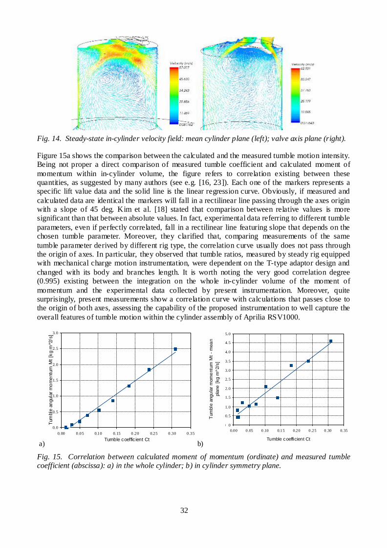
32

Fig. 14. Steady-state in-cylinder velocity field: mean cylinder plane (left); valve axis plane (right).

Figure 15a shows the comparison between the calculated and the measured tumble motion intensity. Being not proper a direct comparison of measured tumble coefficient and calculated moment of momentum within in-cylinder volume, the figure refers to correlation existing between these quantities, as suggested by many authors (see e.g. [16, 23]). Each one of the markers represents a specific lift value data and the solid line is the linear regression curve. Obviously, if measured and calculated data are identical the markers will fall in a rectilinear line passing through the axes origin with a slope of 45 deg. Kim et al. [18] stated that comparison between relative values is more significant than that between absolute values. In fact, experimental data referring to different tumble parameters, even if perfectly correlated, fall in a rectilinear line featuring slope that depends on the chosen tumble parameter. Moreover, they clarified that, comparing measurements of the same tumble parameter derived by different rig type, the correlation curve usually does not pass through the origin of axes. In particular, they observed that tumble ratios, measured by steady rig equipped with mechanical charge motion instrumentation, were dependent on the T-type adaptor design and changed with its body and branches length. It is worth noting the very good correlation degree (0.995) existing between the integration on the whole in-cylinder volume of the moment of momentum and the experimental data collected by present instrumentation. Moreover, quite surprisingly, present measurements show a correlation curve with calculations that passes close to the origin of both axes, assessing the capability of the proposed instrumentation to well capture the overall features of tumble motion within the cylinder assembly of Aprilia RSV1000.

a)

0.0

0.5

1.0

1.5

2.0

2.5

3.0

0.00 0.05 0.10 0.15 0.20 0.25 0.30 0.35Tumble coeffic ient Ct

Tum

ble

angu

lar m

omen

tum

Mt [

kg m

^2/s

]

b)

0.0

0.5

1.0

1.5

2.0

2.5

3.0

3.5

4.0

4.5

5.0

0.00 0 .05 0 .10 0.15 0.20 0 .25 0 .30 0.35

Tumble coefficient Ct

Tum

ble

angu

lar m

omen

tum

Mt -

mea

n pl

ane

[kg

m^2

/s]

Fig. 15. Correlation between calculated moment of momentum (ordinate) and measured tumble coefficient (abscissa): a) in the whole cylinder; b) in cylinder symmetry plane.

33

Figure 15b shows the correlation curve between measurements and the integration of tumble moment of momentum limited to the cylinder symmetry plane. The correlation index is still acceptable (0.967) assessing the capability of cylinder mean plane to be quite representative of the whole tumble motion. However, the spreading of the markers corroborates the need of data for more planes, in order to satisfactory capture charge motion features.

6 Conclusions A mechanical instrumentation featuring a spherical lens-shaped paddle wheel is designed to quickly measure overall intensity of both swirl and tumble in-cylinder charge motion by mean of traditional steady-state discharge-flow test rigs. The sensitivity to tumble motions due to different design of runner-valves-cylinder is experimentally checked on two different engine head of production high-speed motorbike engines. The limited fluid-dynamic blockage of the device affecting discharge-flow coefficient measurements is proven as well. Finally, a comparison with the result of a detailed CFD model is presented to verify the reliability of tumble intensity measurements within a low-medium tumble cylinder assembly. The CFD model, featuring polyhedral grids, is validated both numerically and experimentally. Grid sensitivity study demonstrates the need of 650000 cells with a 4-to-5 near-wall prism-layer within intake runners, ports and whole cylinder to reach discharge-flow coefficient results independent to grid size. As other researchers stated before, the modified Wilcox k- turbulence model predictions are confirmed to be closer to experiments than realizable k- results. Moreover, k- exhibits the property to be less sensitive to grid refinements and to give acceptable results also for very coarse grid computations. The comparison between CFD results and tumble measurements assesses a very good correlation if the overall in-cylinder flow is considered. This stated the capability of present instrumentation to well capture the relevant features of tumble motion, despite its inherent simplicity and structure of tumble, which change between planes perpendicular to vortex axis as evidenced by CFD results.

Acknowledgments Authors acknowledge Roberto Meneghello for the fundamental contribution to the results of reverse-engineering activity and Fabio Zanotto for the CAD modelling work.

References [1] Fujimoto M., Iwai K.; Kataoka M., Tabata M., Effect of combustion chamber shape on tumble

flow, squish-generated flow and burn rate. JSAE Review 2002; 23(3): 291-96. [2] Huang RF., Lin KH., Yeh C-N, Lan J., In-cylinder tumble flows and performance of a

motorcycle engine with circular and elliptic intake ports. Exp Fluids 2009; 46: 165-79. [3] Huang RF., Yang HS., Yeh C-N, In-cylinder flows of a motored four-stroke engine with flat-

crown and slightly concave-crown pistons. Experimental Thermal and Fluid Science 2008; 32 : 1156-67.

[4] Huang RF., Huang CW., Chang SB., Yang HS., Lin TW., Hsu WY., Topological flow evolution in cylinder of a motored engine during intake and compression strokes. Journal o f Fluids and Structures 2005; 20: 105-27.

[5] Lee K., Bae C., Kang K., The effects of tumble and swirl flows on flame propagation in a for-valve S.I. Engine. Applied Thermal Engineering 2007; 27: 2122-30.

[6] Omori S., Iwachido K., Motomochi M., Hirako O., Effect of Intake Port Flow Pattern on the In-Cylinder Tumbling Air Flow in Multi-Valve SI Engines. In: Proceedings of the Internationa l Congress & Exposition; 1991 February; Detroit, MI, USA. SAE Technical Paper 910477.

[7] Heywood JB., Internal Combustion Engine Fundamentals. Singapore: McGraw-Hill Inc.; 1988. [8] Kang KY., Reitz RD., Intake Flow Structure and Swirl Generation in a Four-Valve Heavy-Duty

Diesel Engine. ASME J. Eng. for Gas Turbines Power 2000; 122(4): 570-79.

34

[9] Hong CW., Tarng SD., In-Cylinder Tumble Flow Field Measurements and Predictions. ASME J. Eng. for Gas Turbines Power 2001; 123(1): 139-45.

[10] Kang KY., Reitz RD., The effect of intake valve alignment on swirl generation in a DI diesel engine. Experimental Thermal and Fluid Science 1999; 20(2): 94–103.

[11] Arcoumanis C., Hu Z., Vafidis C., Whitelaw JH., Tumbling Motion: A Mechanism for Turbulence Enhancement in Spark-Ignition Engines. In: Proceedings of International Congress & Exposition; 1990 February; Detroit, MI, USA. SAE Technical Paper 900060.

[12] Brandstätter, W., Johns RJR, Wigley G., The Effect of Inlet Port Geometry on In-Cylinder Flow Structure. 1985; SAE Technical Paper 850499.

[13] Kang KY., Baek JH., LDV Measurement and Analysis of Tumble Formation and Decay in a Four-Valve Engine. Experimental Thermal and Fluid Science 1995; 11: 181-189.

[14] Murali Krishna B., Mallikarajuna JM., Comparative study of in-cylinder tumble flows in an internal combustion engine using different piston shapes-an insight using particle image velocimetry. Exp. Fluids 2010; 48: 863-74.

[15] Yun J. E., Lee J. J., A study on Combine effects between swirl and tumble flow on intake port system in cylinder head. In : Proceedings of FISITA World Automotive Congress; 2000 June, Seoul, Korea. F2000A094.

[16] Godrie P., Zellat M., Simulation of Flow Field Generated by Intake Port-Valve-Cylinder Configurations-Comparison with Measurements and Applications. In: Proceedings o f International Congress & Exposition; 1994 February; Detroit, MI, USA. SAE Technical Paper 940521.

[17] Moore W., Foster W., Lai M.-C., Xie X.-B., Zheng Y., Matsumoto A., Charge motion benefits of valve deactivation to reduce fuel consumption and emission in a GDI, VVA Engine. In: SAE 2011 World Congress & Exhibition, 2011 April, Detroit, MI, USA. SAE Technica l Paper 2011-01-1221.

[18] Kim M., Lee S., Kim W., Tumble Flow Measurements Using Three Different Methods and its Effects on Fuel Economy and Emissions. In: Proceedings of Powertrain & Fluid Systems Conference and Exhibition; 2006 October; Toronto, ON, CANAD. SAE Technical Paper 2006-01-3345.

[19] Algieri A., Bova S., De Bartolo C., Influence of valve lift and throttle angle on intake flow in a high performance four-stroke motorcycle engine. ASME J. Eng. for Gas Turbines Power 2006; 128(4): 934-42.

[20] Gosman AD., Multidimensional Modelling of Cold Flows and Turbulence in Reciprocating Engines. 1985; SAE Technical Paper 850344.

[21] Gosman AD. Ahmed AMY., Measurement and Multidimensional Prediction of Flow in a Axisymmetric Port/Valve Assembly. 1987; SAE Technical Paper 870592.

[22] Dent, JC., Chen A., An Investigation of Steady Flow Through a Curved Inlet Port. In: Proceedings of International Congress & Exposition; 1994 February; Detroit, MI, USA. SAE Technical Paper 940522.

[23] Berfrui B. A., CFD Simulation and Comparison with Measurement of Steady Flow in Intake Ports and Combustion Chambers. In: COMODIA 94: Proceedings of the 3rd Internationa l Symposium on Diagnostics and Modeling of Combustion in Internal Combustion Engines; 1994 July 11-14; Yokohama, Japan. 535-40.

[24] Fuchs TR., Rutland CJ., Intake Flow Effects on Combustion and Emissions in a Diesel Engine. In: Proceedings of the International Congress & Exposition; 1998 February; Detroit, MI, USA. SAE Technical Paper 980508.

35

[25] Ramajo DE., Nigro NM., In-Cylinder Flow Computational Fluid Dynamics Analysis of a Four-Valve Spark Ignition Engine: Comparison Between Steady and Dynamic Tests. ASME J. Eng. for Gas Turbines Power 2010; 132(5): 052804-1-10.

[26] El-Behery SM., Hamed MH., A comparative study of turbulence models performance for separating flow in a planar asymmetric diffuser. Computers & Fluids 2011; 44: 248–57.

[27] So RM., Lai YG., Hwang BC., Second-order near-wall turbulence closure: A review. AIAA J. 1991; 29: 1819-35.

[28] Jia R., Sundén B., Miron P., Léger B., A Numerical and experimental investigation of the slot film-cooling jet with Various Angles. J. Turbomach. 2005; 127: 635-45.

[29] Paul SS., Ormiston SJ., Tachie MF., Experimental and numerical investigation of turbulent cross-flow in a staggered tube bundle. Int. J. Heat and Fluid Flow 2008: 29: 387–414.

[30] Speziale CG, So RMC., Turbulence modeling and simulation. In: Johnson RW, editor. The Handbook of fluid dynamics. Boca Ratom, FL: CRC Press. 1998. p. 14.1-14.111.

[31] Wilcox DC., Turbulence modeling for CFD. La Canada, CA: DCW Industries; 1998. [32] Wallin S., Johansson AV., An explicit algebraic Reynolds stress model for incompressible

and compressible turbulent flows. Journal of Fluid Mechanics 2000; 403: 89–132. [33] Gullman-Strand J., Törnblom O., Lindgren B., Amberg G., Johansson AV., Numerical and

experimental study of separated flow in a plane asymmetric diffuser. Int. J. Heat and Fluid Flow 2004; 25: 451–60.

[34] Bianchi GM., Fontanesi S., On the applications of low-Reynolds cubic k- turbulence models in 3D simulations of ICE intake Flows. In: Proceedings of the International Congress & Exposition; 2003 February; Detroit, MI, USA. SAE Technical Paper 2003-01-0003.

[35] Algieri A., Bova S., De Bartolo C., Nigro A., Numerical and Experimental Analysis of the Intake Flow in a High Performance Four-Stroke Motorcycle Engine: Influence of the Two-Equation Turbulence Models. ASME J. Eng. for Gas Turbines Power 2007; 129: 1095-105.

[36] Shih T-H., Liou WW., Shabbir A., Yang Z., Zhu J., A New k- eddy viscosity model for high Reynolds number turbulent flows-Model development and validation. Comput. Fluids 1995; 24: 227–38.

[37] UNI 10531, (In Italian) Ventilatori industriali - Metodi di prova e condizioni di accettazione (Industrial fans – Test methods and conditions for the acceptance), Milano, Italy; 1995.

[38] Martegani AD., .Lazzaretto A, Taffurelli A., A User’s Guide to the UNI 10531 Standard on Performance Testing of Industrial Fans; 2003, 4 Dec. Document ISO/TC117 No: 306 Annex 3.

[39] Masi M., Toffolo A., Antonello M., Experimental analysis of a motorbike high speed racing engine. Applied Energy 2010; 87: 1641-50.

[40] Zanotto F., Studio sperimentale e numerico dei condotti valvola di scarico di un motore 4 tempi con il supporto di tecniche di ingegneria inversa (in Italian) [MSc thesis]. Padova, Italy: University of Padova; 2011.

[41] Fontana G., Galloni E., Variable valve timing for fuel economy improvement in a small spark ignition engine. Applied Energy 2008; 86: 96-105.

[42] Wolfstein M., The velocity and temperature distribution in one-dimensional flow with turbulence augmentation and pressure gradient. Int. J. Heat Mass Transfer 1969; 12:301-318.

PROCEEDINGS OF ECOS 2012 - THE 25TH INTERNATIONAL CONFERENCE ON

EFFICIENCY, COST, OPTIMIZATION, SIMULATION AND ENVIRONMENTAL IMPACT OF ENERGY SYSTEMS


36

CFD Simulation of Entropy Generation in Pipeline for Steam Transport in Real Industrial Plant

Goran Vučkovića, Gradimir Ilić

b, Mića Vukić

c Milan Banić

d and Gordana Stefanović

e

a University of Niš, Faculty of Mechanical Engineering, Niš, Serbia, [email protected], CA

b University of Niš, Faculty of Mechanical Engineering, Niš, Serbia, [email protected]

c University of Niš, Faculty of Mechanical Engineering, Niš, Serbia, [email protected]

d University of Niš, Faculty of Mechanical Engineering, Niš, Serbia, [email protected] e University of Niš, Faculty of Mechanical Engineering, Niš, Serbia, [email protected]

Abstract:

The success of methods to increase the energy efficiency, to a large extent depends on the efficiency of individual elements, devices and apparatus, which are in the system. Energy efficiency operation of each of the elements of the system can be achieved with good design, which requires knowledge of the processes that take place in the device. The pipelines are an integral part of every industrial plant. The objective of this paper is to illustrate the CFD simulation of entropy generation in one part of pipeline for steam transport in complex industrial plant, like a way of reducing irreversibility production in pipelines. The irreversibility of any fluid flow in pipelines is due to two factors, the transfer of heat across the stream to stream temperature difference (heat transfer irreversibility) and the frictional pressure drop that accompanies the circulation of fluid through the apparatus (fluid friction irreversibility). In this paper the pipeline for steam transport in rubber industry is analysed. The superheated steam at the pressure 10 bar is a fluid that transfers the energy from the steam boiler to the apparatus in the factory. For a defined geometry of pipeline, the model was created, and as results are represented the fields of local entropy generation due to heat transfer and fluid friction, and the total entropy generation in the pipeline. The minimum values of the local entropy generation rate in the steam flow meter (2.801x10

-7 W/m

3K and

6.274x10-7

W/m3K) are obtained in the core of fluid at the straight part of pipeline with constant cross-section.

The maximum values (1.705 W/m3K and 14.360 W/m

3K) are occurs near the wall. In the case of pipe curve

at 90º turns the local entropy generation rate has a minimum values (3.223x10-10

W/m3K and 4.730x10

-10

W/m3K) in the core of stream in the inlet of curve, and maximum values (1.733 W/m

3K and 14.580 W/m

3K)

near the wall due to heat transfer and friction between the fluid and the wall. On the entropy generation has a dominant influence of irreversibility due to friction in comparison to the irreversibility caused by heat transfer.

Keywords:

CFD, entropy generation, energy efficiency, pipeline.

1. Introduction and Background Heat transfer, as a way of thinking and formulation problems, is considerably older than

thermodynamics. The foundation of knowledge of entropy production goes back to Clausius and

Kelvin’s studies on the irreversible aspects of the Second law of thermodynamics. Since then the

theories based on these foundations have rapidly developed [1]. Entropy generation is associated

with thermodynamic irreversibility, which is common in all types of heat transfer processes.

Different sources are responsible for generation of entropy like heat transfer across finite

temperature gradient, characteristic of convective heat transfer, viscous effect etc. Entropy

generation through heat and fluid flow is designed to bridge the gap between three cornerstone

subjects: heat transfer, thermodynamics and fluid mechanics. From historical point of view entropy

generation through heat and fluid flow became a part of engineering thermodynamics in the last

decade of previous century [2].

Flow through pipelines and heating situations find wide applications in industry. Bejan [2] focused

on the different reasons behind entropy generation in applied thermal engineering. Generation of

entropy destroys available work of a system. Therefore, it makes good engineering sense to focus

on irreversibility of heat transfer and fluid flow processes and try to understand the function of

37

entropy generation mechanism. Bejan [3] presented a study of four basic convective heat transfer

phenomena from the unique point of view of entropy generation, and illustrated, in a very modest

way, the place thermodynamics duly occupies in heat transfer. Mahmud and Fraser [1] analyzed

Second law characteristics of heat transfer and fluid flow due to forced convection of steady-

laminar flow of incompressible fluid inside channel with circular cross-section and channel made of

two parallel plates. Different problems are discussed with their entropy generation profiles and heat

transfer irreversibility characteristics. Guo, et all [4] presented the viscous dissipation effect on the

entropy generation for laminar flow region in curved square microchannles is numerically

investigated. Aniline and ethylene glycol are selected as the working fluids. Sahin and Mansour [5]

investigated a numerical solution to the entropy generation in laminar viscous fluid flow through a

circular pipeline, with uniform heat flux at wall boundary condition. Zaharnah and Yilbas [6] the

influence of fluid viscosity on the entropy generation rate is investigated in the pipeline flow at

different wall temperatures. The temperature and flow fields are computed numerically using the

control volume method. It is found that fluid viscosity influences considerably temperature

distribution in the fluid close to the pipeline wall. Yapici et all [7] presented in study the

investigation of the local entropy generation in compressible flow through a suddenly expanding

pipe. Air is used as fluid. To determine the effects of the mass flux, the ambient heat transfer

coefficient and the inlet temperature on the entropy generation rate, the compressible flow is

examined for various cases of these parameters. The flow and temperature fields are computed

numerically with the help of the computational fluid dynamics (CFD) code. In addition to this CFD

code, a computer program has been developed to calculate numerically the entropy generation and

other thermodynamic parameters by using the results of the calculations performed for the flow and

temperature fields. Ko [8] three-dimensional laminar forced convective flow and entropy generation

in a 180-deg curved rectangular duct with longitudinal ribs equipped on the heated wall have been

investigated by numerical methods. The effects of rib size under different flow conditions with

various Dean number and external flux are particularly highlighted. Ko and Ting [9] numerically

analyzed entropy generation for laminar forced convection in curved rectangular ducts and air as the

working fluid under constant heat flux condition; and found that there exists an optimal Dean

number for each aspect ratio, and the optimal Dean number increases as the dimensionless heat flux

increases.

2. Methodology

2.1 Local Rate of Entropy Generation in Convective Heat Transfer

The purpose is to study the volumetric entropy generation rate distribution throughout the fluid in

the pipeline. This requires solution of velocity and temperature fields in the fluid. The governing

equations and the boundary conditions for this steady problem with constant thermophysical

properties are as follows:

Continuity ( 0w ):

0x y zw w wx y z

(1)

Momentum ( 2w w p w ):

2 2 2

2 2 2

x x x x x xx y z

w w w w w wpw w w

x y z x x y z

(2a)

2 2 2

2 2 2

y y y y y y

x y z

w w w w w wpw w w

x y z y x y z

(2b)

38

2 2 2

2 2 2

z z z z z zx y z

w w w w w wpw w w

x y z z x y z

(2c)

Energy ( 2pc w T T ):

2 2 2

2 2 2p x y z

T T T T T Tc w w w

x y z x y z

(3)

In the fluid flow, irreversibility arises due to the heat transfer and the viscous effects of the fluid.

The entropy generation rate can be expressed as the sum of contributions due to thermal and viscous

effects, and thus it depends functionally on the local values of temperature and velocity in the

domain of interest. In these systems, when both temperature and velocity fields are known, the local

or volumetric entropy generation rate at each point can be calculated as follows equation, in tensor

notation [10]:

2

2genS TTT

, (4)

or in development form:

22 2

2gen

T T TS

x y z TT

(5)

In equitation (3) and (5) is the viscous dissipation function, which is [11]:

2 2 22 22

2y y yx x xz z z

w w ww w ww w w

x y z x y y z z x

(6)

2

2

3

yx zww w

x y z

.

The first and second term on the right side in equitation (4) and (5) represent, respectively, the local

entropy generation rate due to heat transfer and fluid friction.

In accordance with the foregoing, equation (5) can be symbolically represent in the form:

gen gen genHT FF

S S S , (7)

The total entropy generation rate over the volume can be calculated as follows [7]:

gen gen

V

S S dxdydz . (8)

Based on the known values of entropy generation can be by applying the theorem of lost available

work, or Gouy-Stodola theorem, determine the amount of exergy destruction. The destruction of

exergy is proportional to the value of the generated entropy, where the coefficient of proportionality

is the reference temperature [12]:

0D genE T S (9)

Owing to exergy destruction, but and exergy loss, the exergy rate at the outlet is less than the exergy

rate at the inlet. These exergy quantities are related by the exergy rate balance, which at steady state

can be expressed as [13]:

39

i e D LE E E E (10)

The rate of exergy loss equals the rate of exergy transfer associated with heat transfer, and is thus

given by [10]:

01

e

L q

bi

TE E q dL

T

(11)

where is:

, 0l f lq k t t (12)

To obtain the information which irreversibility dominated for entropy generation, due to heat

transfer or fluid friction, Bejan was define dimensionless parameter - Irreversibility distribution

ratio. The irreversibility distribution ratio is equal to the ratio of entropy generation due to fluid

friction to heat transfer [2]:

genFF

genHT

S

S

. (13)

Heat transfer irreversibility dominates over fluid friction irreversibility for 0 and fluid friction

dominates when . For 1 , both the heat transfer and fluid friction have the same contribution

for generating entropy In the case 1 or entropy generation is occurs only due to friction.

As an alternative irreversibility distribution ratio, defined Bejan number [1] which describes the

contribution of heat transfer entropy on overall entropy generation, is defined as [8]:

Be

genHT

gen

S

S

, (14)

Bejan number ranges from 0 to 1. Accordingly, Be 1 is the limit at which the heat transfer

irreversibility dominates, Be 0 is the opposite limit at which the irreversibility is dominated by

fluid friction effects, and Be 0.5 is the case in which the heat transfer and fluid friction entropy

generation rates are equal. [1, 7].

Using equations (7) and (13) can be established a relationship between Bejan's number and

irreversibility distribution ratio [1]:

1Be

1

. (15)

2.2 Computational Procedure

The general theory of fluid motion is too difficult to enable the user to attack arbitrary geometric

configurations. It is possible to apply merely numerical techniques to arbitrary geometries.

Computational fluid dynamics turns out the methods are applicable to a number of systems of

equations which fall under the category of conservation laws. Therefore, a suitable numerical

method and/or computational fluid dynamics code is frequently used to solve the governing

equations in this field. The CFD code is the program by which fluid flow can be predicted through

arbitrary geometries, giving such information as flow speed, pressures, residence times, flow

patterns, etc. The main advantage of this approach is in its potential for reducing the extent and

number of experiments required to describe such types of flow.

40

2.2.1 Calculation Tools

The ANSYS CFX 13 program was chosen as the CFD computer code to calculate entropy

generation in a steam pipeline. The software was chosen due the ease with which the analysis model

can be created, and because the software allows input of new equations necessary for calculation of

entropy generation rate. Furthermore, ANSYS CFX computer code enables the definition of wall

heat transfer coefficient as a user function, which parameters are solved during the solving of fluid

flow equations. The ANSYS CFX computer code uses a finite-volume procedure to solve the

Navier-Stokes equations of fluid flow in primitive variables such as velocity (wx, wy, wz) and

pressure. Noted computer code includes various turbulence models [14] among which k-ε model

was selected in entropy generation rate calculation. k-ε model calculates turbulent viscosity (μt) as a

function of turbulent kinetic energy (k) and turbulence dissipation rate (ε). Fluid flow equations

include the viscous term in order to calculate entropy generation rate due to fluid friction.

The thermo-physical properties of steam were adopted according to the International Association

for the Properties of Water and Steam (IAPWS) equation of state, incorporated into ANSYS CFX

computer code. In ANSYS CFX, the analytical equation of state is used to transfer properties into

tabular form. These IAPWS tables are defined in terms of pressure and temperature, which are then

inverted to evaluate states in terms of other property combinations, such as pressure/enthalpy or

entropy/enthalpy [14].

As ANSYS CFX calculates automatically derivates of temperature and velocity components, the

expressions necessary to calculate volumetric entropy generation were inserted into solver by the

CFX Command Language (CCL).

The finite element mesh was created from pipeline geometrical model by patch confirming method.

Boundary layer was inflated with 20 layers with total thickness of 3 mm. The finite element mesh

has 3508655 nodes which form 2662769 tetrahedrons and 5972280 wedge elements. All mesh

quality parameters (Orthogonality angle, Expansion factor and Aspect ratio) are in permissible

range for a double precision solver.

2.2.2 Simulation Values

Steam pipeline boundary conditions were defined based on actual measurement of mass flow rate,

temperature and pressure at inlet and outlet. The simulation parameters are given in Table 1.

Table 1. Overview of simulation parameters

Parameters Value/setting

Analysis type steady state

Steam properties IAPWS IF97

Thermodynamic state gas

Temperature of the surrounding, oC 10

Reference pressure, atm 0

Heat transfer model total energy

Inlet flow regime subsonic

Inlet volumetric flow rate, m3/h 150/400

Inlet steam temperature, oC 181.4/182.6

Inlet turbulence medium intensity and eddy viscosity ratio

Outlet flow regime subsonic

Outlet static pressure, bar 9.85/9.25

Wall mass and momentum no slip wall

Wall roughness, mm 0.2

Wall heat transfer coefficient, W/m2K calculated during solve

1

Turbulence numerics high resolution

Advection scheme high resolution

Execution control double precision

Convergence criteria - Residual Target RMS ≤ 10-5

1The wall heat transfer coefficient was calculated during the solve procedure based on equation:

41

1

1 1ln ln

2 2

is is is ew is

ex is ew pw iw iw in

kd d d d d

d d d

(16)

3. Background of Industrial Plant and Pipeline Geometry The energy system in a representative industrial plant, Fig. 1, consists of four parts: Energy supply

sector (EN), Factory 1 (F1), Factory 2 (F2) and Engineering department (IN).

Energy supply sector is a part of the factory complex where chemical and thermal treatment of

water is being carried out, and superheated steam for their own use and supply of all other

consumers is produced.

The boiler produces superheated steam at the pressure of 10 bars, which is then distributed to

factories 1 and 2, and partly reduced at lower pressures in accordance with the needs of consumers.

Factory 1 is the largest consumer of energy in the whole complex and is supplied with energy using

the superheated steam at the pressure of 10 bars. The focus point in this paper is a pipeline in which

distributed superheated steam at 10 bars from Energy supply sector to Factory 1.

Fig. 1. Flow diagram of the representative industrial plant

The present steam pipeline, Fig. 2, is made of steel with a nominal diameter of DN 150 with total

length of 148.7 m. In one part of the pipeline cross-section is reduced for the steam flow meter.

Pipeline contains more curves at angle of 90o and two elements for compensate expansion due to

temperature change.

Fig. 2. Real steam pipeline

42

The pipeline is to reduce heat losses to the environment covered with insulation material thickness

of 80 mm. Due to that pipeline mainly located in open space, insulation material is protected by

aluminium tin. From the inside area pipeline is not an ideal smooth, but has a certain roughness,

which is characterized with roughness height 0.2 mm.

4. Results and Discussion

4.1 Analysis Results for the whole Steam Pipeline

The results of numerical calculations for the whole pipeline are given in Table 2. From the collected

results, it can be concluded that with increasing volumetric flow rate of 2.67 times, respectively

with 150 m3/h to 400 m

3/h, the total entropy generated due to irreversibility in the pipeline increases

more than 10 times, and in the same amount increases exergy destruction. The dominant effect of

entropy generation is due by fluid friction. On the other hand, at higher volumetric flow rates

decreases the value of entropy generation due to the irreversibility caused by convective heat

transfer, but to a much lesser extent than the increase of entropy generation by friction of fluids.

The dominance of irreversibility due to fluid friction is expressed through the values of

irreversibility distribution ratio, which in both cases is greater than 1 (3.200 and 120.464). For the

higher volumetric flow rate (Case 2), irreversibility distribution ratio has a far higher value,

120.464. Also, both the values for the dimensionless criterion, Bejan's number, are close to zero

(0.238 and 0.00824), indicating little impact of irreversibility due to convective heat transfer in the

steam flow of 150 m3/h, and almost insignificant impact of irreversibility due to convective heat

transfer in the steam flow of 400 m3/h.

Table 2. Overview of results for whole steam pipeline

Parameters Units Case 1 Case 2

m3/h 150.00 400.00

pi (measured) bar 10.000 9.420

pi (simulation) bar 9.883 9.277

pe (measured) bar 9.850 9.250

pe (simulation) bar 9.850 9.250

Ti (measured) K 454.540 455.740

Te (simulation) K 451.823 454.555

To K 283.140 283.140

T0 K 298.150 298.150

W/K 0.0003755 0.003792

W/K 8.942e-5 3.122e-5

W/K 0.0002861 0.003761

- 3.200 120.464

Be - 0.238 0.00824

k W/m2K 0.307597 0.308593

tz K 452.90 455.01

W -1,309.68 -1,332.24

W 0.112 1.121

4.2 Analysis Numerical Results for Local Entropy Generation and Bejan Number for Characteristics Parts of Steam Pipeline

In general, the local entropy generation rate is maximal, as expected, near the wall due to heat

transfer and friction between the fluid and the wall. The temperature of the fluid will decrease

gradually towards the pipe wall and outlet, and the temperature gradients in the radial and axial

directions will occur, which in turn will increase the local entropy generation rate.

Furthermore, the local entropy generation rate is maximal at the flow meter (Fig. 3) and in pipeline

curves (Fig. 5). In this paper we analyzed first curve at the pipeline and fluid flow meter (Fig. 2).

43

As known, in a pipe flow, the cross-section contraction in flow meter accelerates fluid, and the

sudden expansion in the pipe produces the high velocity gradients which also increase the local

entropy generation rate. It is obvious from Fig. 3 that local entropy generation rate increases with

the increase in fluid mass flow rate i.e. fluid velocity. The minimum values of the local entropy

generation rate in the both cases (2.801x10-7

W/m3K and 6.274x10

-7 W/m

3K) are obtained in the

core of fluid at the straight part of pipeline with constant cross-section. The maximum values (1.705

W/m3K and 14.360 W/m

3K) are occurs near the wall.

a) volumetric flow rate 150 m3/h b) volumetric flow rate 400 m

3/h

Fig. 3. Local entropy generation rate at flow meter (logarithmic)

Fig. 4 shows the distribution of Bejan number in steam flow meter. As Bejan number values are

smaller than 0.8 for the lower mass flow rate, and smaller than 0.2 for higher mass flow rate.

In the first case in very small area (only part of red zone, 0.5 Be ≤ 0.7882) irreversibility from

convective heat transfer is dominate for local entropy generation. In the point where is Be=0.5

irreversibility from convective heat transfer and fluid friction are equal for local entropy generation.

In the other part of flow meter values of Bejan number is very close to zero, it is clear that

irreversibility from heat transfer has less influence on resultant local entropy generation rate then

irreversibility from fluid friction.

In the second case, all values of Bejan number are smaller than 0.5 and for these reason, in whole

part of flow meter irreversibility from fluid friction is dominate for entropy generation.


3/h

Fig. 4. Bejan number at flow meter (logarithmic)

The velocity change in curves and the consequent change in velocity gradients also increases the

local entropy generation rate (Fig. 5). Again, the local entropy generation rate increases with the

increase in fluid mass flow rate. The local entropy generation rate in the both cases has a minimum

values (3.223x10-10

W/m3K and 4.730x10

-10 W/m

3K) in the core of stream in the inlet of curve, and

maximum values (1.733 W/m3K and 14.580 W/m

3K) near the wall due to heat transfer and friction

between the fluid and the wall.

Fig. 6 shows the distribution of Bejan number in pipeline curve.

As maximal Bejan number values are relatively high (0.9984) for the lower mass flow rate is clear

that irreversibility from heat transfer has dominant influence on resultant local entropy generation.

But this value and values higher than 0.5 valid only in very small area having in mind that the red

genS

genS

genS

genS

44

zone includes values for Bejan number from 0.1990 to 0.9984. In the point where is Be=0.5

irreversibility from convective heat transfer and fluid friction are equal for local entropy generation.

In the other part of pipe curves values of Bejan number is very close to zero, it is clear that

irreversibility from heat transfer has less influence on resultant local entropy generation rate then

irreversibility from fluid friction.


3/h

Fig. 5. Local entropy generation rate at pipeline curve (logarithmic)

In the second case, all values of Bejan number are smaller than 0.5 and for these reason, in whole

part of pipe curve irreversibility from fluid friction is dominate for entropy generation. Furthermore,

no matter what heat transfer losses are greater for higher volumetric flow rate, influence of

irreversibility from heat transfer on entropy generation is decreases with increase fluid flow.


3/h

Fig. 6. Bejan number at pipeline curve (logarithmic)

5. Conclusions The paper presents a numerical simulation of entropy generation in the real pipeline superheated

steam. The results of numerical simulation show good agreement with measured data in regard to

temperature. The inability to predict pressure drop is a consequence of relatively coarse mesh in the

core of the pipeline. Due to relatively coarse mesh the CFX solver cannot accurately calculate fluid

friction losses and thus irreversibility from fluid friction. Noted trade-off in coarse mesh in central

fluid region was introduced to decrease the computational resources necessary to perform

calculations i.e. decrease of time necessary to perform calculations to a reasonable frame.

Regardless of the above simplifications, examples of steam flow meter and pipe curve, it is shown

genS

genS

45

that the irreversibility of friction far more influence on the generation of entropy than irreversibility

from heat transfer, and therefore on the loss of available work or exergy destruction. Having in

mind previous, the general conclusion is that in order to increase the energy efficiency of the system

should significantly decrease the friction between the pipe wall and fluid.

Nomenclature Be - Bejan number

E - exergy flow rate, W

d - diameter, m

k - heat transfer coefficient, W/(m2K)

p - pressure, bar

q - heat transfer rate per unit of length, W/m

Q - heat transfer rate, W

genS - entropy generation rate, W/K

genS - local entropy generation rate, W/(m3K)

t - temperature, oC

T - temperature, K

V - volumetric flow rare, m3/h

w - velocity, m/s

Greek symbols

- convective heat transfer coefficient, W/(m2K)

- irreversibility distribution ratio

- viscous dissipation function, s-2

- thermal conductivity, W/(mK)

Greek symbols (continue)

- viscosity, kg/(sm)

- density, kg/m3

Subscripts

b - boundary

D - destruction

e - outlet

ew - external wall

ex - external

FF - fluid friction

HT - heat transfer

i - inlet

in - internal

is - isolation

iw - internal wall

L - loss

o - environment

pw - pipe wall

q - heat transfer

0 - reference state

References [1] Mahmud S., Fraser A.R.: The Second Low Analysis in Fundamental Convective Heat Transfer

Problems, Thermal Science 2003; 42: 177-86.

[2] Bejan A: Entropy Generation through Heat and Fluid Flow, John Wiley&Sons; 1982.

[3] Bejan A.: A Study of Entropy Generation in Fundamental Convective Heat Transfer, Journal of

Heat Transfer 1979; 101: 718-25.

[4] Guo J., Xu M., Cai J., Huai X.: Viscousn Dissipation Effect on Entropy Generation in Curved

Square Microchannels, Energy 2011; 33: 5416-23.

[5] Sahin Z.A., Mansour B.R.: Entropy Generation in Laminar Fluid Flow through a Circular Pipe,

Entropy 2003; 5: 404-16.

[6] Zaharnah A.T., Yilbas S.B.: Thermal Analysis in Pipe Flow: Influence of Variable Viscosity

on Entropy Generation, Entropy 2004; 6: 344-63.

[7] Yapici H., Kayatas N., Kahraman N., Baştürk G.: Numerical Study on Local Entropy

Generation in Compressible Flow through a Suddenly Expanding Pipe, Entropy 2005; 7: 38-67

[8] Ko H.T.: Numerical Investigation on Laminar Forced Convection and Entropy Generation in a

Curved Rectangular Duct with Longitudinal Ribs Mounted on Heated Wall Ducts, Thermal

Science 2006; 45: 390-404.

46

[9] Ko H.T., Ting K.: Entropy Generation and Optimal Analysis for Laminar Forced Convection

in Curved Rectangular Ducts: A Numerical Study, Thermal Sciences 2006; 45(2): 138-50.

[10] Bejan A., Tsatsaronis G., Moran M.: Thermal Design and Optimization, New York: John

Wiley&Sons; 1996.

[11] Bird B., Steward W., Lightfoot E.: Transport Phenomena, John Wiley&Sons; 2002.

[12] Szargut J., Morris D.R, Steward F.R.: Exergy Analysis of Thermal, Chemical, and

Metallurgical Processes, New York: Hemisphere Publishing Corporation; 1988.

[13] Edited by Frangopoulos C.: Exergy, Energy System Analysis and Optimization - Exergy and

Thermodynamic Analysis, Vol. 1, EOLSS Publishers Co. Ltd; 2009.

[14] ANSYS CFX 13.0, Theory manual.



47

Feasibility Study of Turbo expander Installation in City Gate Station

Navid Zehtabiyan Rezaiea, Majid Saffar-Avvalb

a Amirkabir University of Technology, Tehran, Iran, [email protected] b Amirkabir University of Technology, Tehran, Iran, [email protected],CA

Abstract: Natural gas pressure has to be increased in natural gas distribution network; meanwhile, before entering the low-pressure lines, this high pressure must be reduced. Pressure let-down in city gate stations is traditionally performed as natural gas passes through a throttle valve, although this method is simple, a considerable irreversibility is imposed to the system. A turbo expander can be used as an alternative way for reducing the gas pressure. The generated mechanical power may be used to produce electricity or drive a compressor. As natural gas flow rate varies during the year, the turbo expander almost operates in off-design conditions. The generated power is evaluated for each day of the year. The study has been applied for Takestan, Iran city gate station with nominal flow rate of 20000 cubic meters per hour. The recovered annual electrical energy is about 1104737 kWh and the project is economic for interest rate up to 18%. Keywords: City gate stations, Natural gas, Pressure reduction, Turbo expander.

1. Introduction Nominal gas pressure in distribution pipelines is about 5-7 MPa, there are several stations for reduction of natural gas pressure, the first step in gas pressure let-down is performed in the city gate station. The process includes the natural gas expansion in a throttle valve, which decreases the pressure and temperature of the gas. Natural gas pre-heating is necessary to avoid condensation and a fraction of pipe gas is burned for this purpose. Replacing the throttle valve with a turbine is an approach to decrease the entropy generation in city gate stations as well as in natural gas distribution system. Replacement of throttle valve with turbo expander does not mean that the throttle valve is eliminated. The turbo expander is installed in parallel with the former system, to avoid any interruptions in gas distribution as a result of turbo expander failure. As stated in [1], turbo expanders were first installed in 1980s in San Diego, Memphis, Stockbridge and Hamilton New Jersey. Joining the turbo expander and fuel cell was first done in 2008 in Toronto Canada. Combination of turbo expanders installed in London natural gas distribution system with bio-fuel burning generator was started in 2009 and was expected to produce 20 MW. Mirandola and Minca [2] showed that for an inlet pressure of 1.13-5.1 MPa and an outlet pressure of 0.15-0.6 MPa, with design flows varying from 5000 to 30000 Nm3/h, a power recovery of about 300-1400 kW is expected. Mirandola and Macor [3] analysed the real data from a prototype built in Ravenna Italy in 1987. Pozivil [4] simulated a natural gas station in Czech Republic. This analysis showed that the temperature drop in the turbo expander will be greater than throttle valve and is about 1.5-2 C per kPa depending on gas composition. The outlet temperature was maintained at 3 C where the inlet and outlet pressures varied from 4.5 to 6.3 MPa and 1.4-2.3 MPa respectively. The flow rate was 60000 Nm3/h and was assumed to be fixed. The study [5] was made for Shahrekord, Iran city gate station having nominal flow rate of 120000 Nm3/h. Average values for flow rates were used for each month, where the monthly flow rates varied from 5 to 40 million cubic meters. The inlet pressure varied from 4.9 to 5.5 MPa, where the outlet pressure was assumed to be 1.8 MPa and fixed. Inlet and outlet temperatures were assumed to

48

be fixed. It was shown that the flow rate of pre-heater is 0.32% of total flow and power recovery was about 0.15-1.18 GWh per month. Rahman [6] studied a number of natural gas wells and pressure reduction stations. It was shown that the power recovery at wellhead is in the range of 150-500 kW and it is about 200 kW to 5 MW in pressure reduction stations.

2. Mathematical modelling of turbo expander Turbo expander is designed to adjust the nominal flow rate of the city gate station as the flow rate varies during the year and it is often less than the nominal flow rate. Inlet pressure and temperature are usually constant. Outlet pressure of the city gate station is an important factor and it shouldn’t be less than 1.7 MPa. If the turbo expander results an outlet pressure less than 1.7 MPa, the aim of the city gate station is missed. Since flow rate variation will cause the outlet pressure variation, an outlet pressure more than 1.7 MPa is selected. Outlet temperature is controlled through generated power and outlet pressure. The main point is that this temperature should always be greater that the dew point of natural at outlet pressure. The composition of natural gas has to be considered as well.

Table 1. Selected natural gas composition for calculations Constituent Mole fraction, xi Molecular weight, Mi Mass fraction, yi Methane 0.8900 16.0400 0.8044 Ethane 0.0410 30.0700 0.0695 Propane 0.0120 44.1000 0.0298 Nitrogen 0.0500 28.0100 0.0789 Carbon dioxide 0.0070 44.0100 0.0174

2.1. Design of turbo expander According to [7] the important parameters in turbo expander design are

4

3)(

076.0

h

QNN s , (1)

QhDDs

41

2 )(36.2 . (2)

Where N shaft speed, rpm Q volumetric flow, m3/s

h ideal enthalpy differential, kJ/kg D2 blade tip diameter, m Radial turbo expanders are more sufficient for natural gas application. According to [7] the efficiency of radial turbo expanders as a function of specific speed, Ns is illustrated in Fig. 1. It is evident that the turbine efficiency is not solely a function of specific speed, but using the diagram offers a primary approach in feasibility studies with many unknown factors. Exact values must be calculated in detailed designs afterwards. One needs to find shaft rotational speed to calculate specific shaft speed. Reference [7] specifies the rotational speed to be a function of estimated shaft power with an efficiency of 0.8 for the turbo expander in Fig. 2. Same reference also presents a diagram that helps to estimate the turbo expander blade tip speed and consequently blade diameter in Fig. 3.

49

Fig. 1. Radial turbo expanders efficiency as a function of specific speed Ns .

Fig. 2. Shaft rotational speed as a function of estimated shaft power.

Fig. 3. Blade tip speed to spouting velocity as a function of specific speed.

Spouting velocity is defined in [7] as

.57.440 hC (3) Where

h ideal enthalpy differential, kJ/kg

50

Flow rate variation over the year is an important issue. It may result an outlet pressure not equal to the design outlet pressure. Choosing a reliable safety factor for the outlet pressure, leads to the design outlet pressure equal to 2.75 MPa, while a throttle valve is placed after the turbo expander to give a pressure equal to 1.7 MPa leaving the city gate station. Fig. 4 shows the new station schematically.

Fig. 4. Schematic form of city gate station with turbo expander.

According to [8] the dew point of natural gas can be predicted by

)3276.36(95 285.0PTdp . (4)

Where P pressure, MPa For an outlet pressure of 2.75 MPa, the dew point is 10 C, where a throttle valve is installed after the turbo expander. The dew point temperature of natural gas after the throttle valve is 6.11 C. Taking advantage of other studies about throttle valve analysis, leads to Ardali and Heybatian [5] who claim that natural gas temperature, drops 18 C passing through the throttle valve, so the outlet temperature of the turbo expander is expected to be 24.11 C instead of 10 C. Inlet pressure is assumed constant and equal to 5.5 MPa. By making a comparison of [5] with this study, it is found that there will be 44.78 C temperature drop in the turbo expander so the inlet temperature must be 68.88 C to ensure the outlet temperature. Ardali and Heybatian [5] also state that the flow rate of pre-heater is 0.32% of the total flow. This study showed that the flow rate of the pre-heater will be 0.2268% of the total flow which is reasonable comparing to [5].

2.2. Off-Design analysis Fig. 5 shows the daily variation of flow rate during the year. This variation will affect the performance of the turbine and must be accounted. It has to be mentioned, natural gas is treated as an ideal solution and a real gas. It is essential to use an equation of state in order to study the process under off-design conditions. In some equations of state such as Redlich-Kwong, despite their complexity of calculations the results are not too far away from the results obtained by ideal gas assumption.

51

Fig. 5. Variation of gas flow rate during the year.

Because of the flow rate variation, the efficiency of the turbo expander is usually different from the design value. Prediction of efficiency changes is made by using the results of [7]. Fig. 6 shows the ratio of efficiency of the turbo expander to design efficiency as a function of ratio of flow rate to design flow rate.

Fig. 6. Efficiency of turbo expander in varying flow rate presented by Atlas Copco.

As mentioned above, outlet pressure differs from the design value as the flow rate is different from design flow. According to [9] the ratio of off-design outlet pressure to design outlet pressure can be calculated by relation

52

. (5)

Where U tip velocity in off-design conditions, m/s Udesign tip velocity in design conditions, m/s efficiency in off-design conditions design efficiency in design conditions

cp specific heat, kJ/(kg K) Tin inlet temperature, K cp/cv

The whole design and off-design process can be seen in Fig. 7.

Fig. 7. Design and off-design process.

12

12

..1

..1

inpDesign

Design

inp

outDesign

out

TcU

TcU

PP

53

3. Results and economic analysis Fig. 8 represents the daily generated power during the year. The energy produced in a year is calculated 1104737 kWh by integration. It is assumed that the generator is DC and invertor produces AC electric to sell. The income due to electric power selling is 46.230 thousand dollars. The capital cost including turbo expander price and installation costs is about 184.56 thousand dollars. Annual costs comprising pre-heater gas burning cost and operation and maintenance costs are estimated 6.8 and 1.8 thousand dollars respectively. Fig. 9 represents the pre-heater gas consumption which equals to 157238 cubic meters of natural gas in the year. Assuming a lifetime of 15 years for the project the IRR1 equals to 18% according to [10].

Fig. 8. Generated power in each day of year.

Fig. 9. Monthly pre-heater gas consumption.

1 Internal rate of return

54

4. Conclusion This feasibility study with some simplifying assumptions reveals interesting results about Takestan C.G.S. The variation of flow rate of this station causes a considerable variation in power production. Although the power output is acceptable in Iran winter, with increase in flow rate, the outlet temperature of the turbo expander is much higher than expected, because of the safety factors selected. The pre-heater consumes 157238 cubic meters of natural gas and 1104737 kWh of electrical energy is recovered in the year. The internal rate of return of the project is 18%. The average efficiency of turbo expander is 67.79 % which is less that the design value because of the variation in flow rates. These variations in flow rate are not considered in other studies but the effect is not negligible particularly for economic investigations.

Nomenclature Co spouting velocity, m/s cp specific heat, kJ/(kg K) D2 blade tip diameter, m Ds specific diameter

h ideal enthalpy differential, kJ/kg N shaft speed, rpm Ns specific speed P pressure, MPa Q volumetric flow, m3/s T temperature, °C U tip velocity, m/s w specific work, kJ/kg Greek symbols efficiency

Subscripts and superscripts dp Dew point

References [1] Rheuban J., Turbo Expanders: Harnessing the Hidden Potential of Our Natural Gas Distribution

System. Article. 2009. Available at: <http://jacobrheuban.com/2009/03/09> [accessed 29.4.2011].

[2] Mirandola A., Minca L., Energy Recovery by Expansion of High Pressure Natural Gas. In: Proceedings of the 21st Intersociety Energy Conversion Engineering Conference; 1986 Aug; San Diego, California.

[3] Mirandola A., Macor A., Experimental Analysis of an Energy Recovery Plant by Expansion o f Natural Gas. In: Proceedings of the 23rd Intersociety Energy Conversion Engineering Conference; 1988 Aug; Denver, Colorado.

[4] Poživil J., Use of Expansion Turbines in Natural Gas Pressure Reduction Stations. Acta Montanistica Slovaca 2004.

55

[5] Ardali E.K., Heybatian E., Energy regeneration in natural gas pressure reduction stations by use of turbo expanders; evaluation of available potential in Iran . In: Proceedings of the 24th world gas conference; 2009 Oct; Buenos Aires , Argentina.

[6] Rahman M.M., Power Generation from Pressure Reduction in the Natural Gas Supply chain in Bangladesh. Journal of Mechanical Engineering 2010.

[7] Bloch H., Soares C., Turbo expander and process application.Butterworth-Heine; 2001. [8] Fattah K.A.A,Evaluation of empirical correlation for natural gas hydrate prediction. Oil and gas

businesses. 2004. [9] Montazerin N., Turbomachines (In Persian). Amirkabir University Publications. 1999. p.88-98. [10] Kreith F., Engineering economics and project management. In: Kreith F, Goswami Y, editors.

The Mechanical Engineering Handbook Series. CRC press. 2004. p. 2121-2180. [11] Data sheet from Takestan city gate station.



56

GTL and RME Combustion Analysis in a Transparent CI Engine by means of IR Digital

Imaging

Ezio Mancaruso, Luigi Sequino, Bianca Maria Vaglieco

Istituto Motori - CNR, Naples, Italy, [email protected]

Abstract: In the present paper, infrared (IR) measurements were performed in order to study the behaviour of biofuels combustion in a transparent Euro 5 diesel engine operating in premixed mode. Commercial diesel fuel (REF) Gas To Liquid (GTL) and Rapeseed Methyl Ester (RME) biofuels have been used. An elongated single cylinder transparent engine equipped with the multi-cylinder head of commercial passenger car and common rail (CR) injection system was used. A sapphire window was set in the bottom of the combustion chamber, and a sapphire ring was placed in the upper part of the cylinder. Measurements were carried out through both accesses by means of high-speed infrared digital imaging system. IR camera was able to detect the emitted light in the wavelength range 1.5-5 m. In a previous paper UV and visible cameras were used, infrared imaging allowed acquiring larger amount of information than those experiments. In particular the IR camera was used for the characterization of injection and combustion process. Analysing the IR images, it was possible to identify clearly the seven jets of vaporized fuel that react with air in the bowl. During the late combustion phase, the IR image showed a good capability to follow the hot burned gas both in the bowl and above the piston. The IR camera has shown high sensibility permitting to follow carefully the soot oxidation process within the cylinder. The GTL shows an advance of about 2°CA in the evolution of combustion process with respect to the RME. On the contrary a longer chemical activity has been detected for the latter biofuel. Finally, the IR camera was revealed very useful tool to characterize the combustion process for long time allowing high quality of the results. Images of the reactions that happen in the combustion chamber and above the piston head were clearly acquired even if the optical windows were obscured by the soot produced from the previous combustion cycles.

Keywords: Biofuels, In-cylinder combustion analysis, Infrared digital imaging.

1. Introduction

Nowadays, one of the possible solutions to make cleaner and more efficient the internal combustion engine (ICE) seems to be the use of biofuels. The fast reduction of fossil fuel resources and their contribution to environmental pollution from ICE, and the increasing request for efficient and eco-friendly energy management have led to an increase in interest among researchers on study combustion characteristics of alternative fuels. Their blends in a certain percentage can be used without modification of engine structure. In particular, great attention is paid to the 1st and 2nd generation of biodiesel. The former is obtained from vegetable resources; it is commonly referred to as FAME (Fatty-Acid Methyl Esters). Its performance is quite similar to those of diesel, in particular, its main characteristic is the higher content of O2 with respect to conventional fuels. On the other hand, moral-social debates are in place because its derivation from edible oil and interferences with the human food chain [1]. The 2nd generation of biodiesel, is produced by the Fischer-Tropsch synthesis process, able to produce liquid fuels from the so-called syngas. It is usually indicated as xTL, where 'x' denotes the specific source feedstock and TL (to Liquid) the conversion to liquid state. The input feedstock can be either renewable Biomass (hence BTL) or fossil fuels, as natural Gas (GTL) or Coal (CTL). Furthermore, the chemical origin of the xTL fuels provides them better combustion characteristic as attitude to autoignition and stability in the

57

chemical composition than FAME, which is essentially driven by the synthesis process itself and not by the baseline feedstock [2, 3].

Moreover, in the last decades, the development of high performance devices and their application in the research fields has provided new techniques suitable for the monitoring of natural phenomena. In the motorist area, the growing attention on these methods is motivated by the need to achieve a more precise description of the processes occurring in the combustion chamber, in order to implement new optimized control methods assuring more efficient and clean combustion systems. Optical diagnostic strongly benefits from technological innovation; the microscopic and macroscopic analysis of the in-cylinder processes gives the possibility to collect significant information. In particular, the opportunity to inspect the phenomena in the infrared (IR) range makes it possible to investigate an area, outside the visible spectrum, where a lot of reactions take place. Each body with a temperature higher than 0 K emits energy, as an electromagnetic radiation, in the whole spectral range from the ultraviolet (UV) up to the infrared (IR). The visible range goes from 380 to 750 nm, so human eyes can't detect energy emitted at higher or lower wavelength. Infrared cameras can detect radiation with a wavelength longer than 750 nm, the infrared range goes from 750 nm to 1000 m and it is divided in Near Infrared (0.78 - 3 m), Mid Infrared (3 - 50 m) and Far Infrared (50 - 1000 m) [4]. The use of infrared cameras in a diesel engine with the aim to gather information about its functioning has many benefits; the main challenge in this field is the definition of the most representative flame signals and to derive the meaningful information required to diagnose the state of a flame. Fuel vapour is not easily observed in the visible wavelength range but is well resolved in the infrared region [5]. In the IR range it is also possible to capture the radiation emitted by species of low-temperature reactions prior to running into rapid heat-releasing reactions [6]. Parker et al. monitored soot formation in the near-infrared for a diesel spray, observing that 9.4 m was an appropriate wavelength for quantitative measurements of soot mass in the spray [7]. Moreover, filtering images from combustion chamber in the IR range allows eliminating the effects due to other substances; it is so possible to study better the stability of combustion [8]. Finally, more information of the energy released are obtained and for a longer time period. However, it is important to consider some limitations and shortfalls of current infrared technologies. In fact, for phenomenon as rapid as combustion process, only little image resolution is available for the high acquisition frequency needed. Moreover, some hot gases, such as oxygen and nitrogen, are mostly transparent in the infrared wavelengths due to their low emissivity. So the temperature measurements will consider the radiation transmitted through these gases rather than the direct radiation emitted by flames, causing difficulties in determination of temperatures [5-8].

This paper deals with the analysis of combustion process in a transparent Euro5 diesel engine operating in premixed mode. The investigation of the phenomena occurring in the combustion chamber is made through IR digital imaging. A single cylinder engine equipped with the head of a Euro5 production engine has been used. A multi injection strategy, consisting of a pilot and a main injection, has been performed with last generation high pressure Common Rail (CR) injection system. IR images have been acquired from two different views: one from the bottom of the cylinder and the other from the side; image luminosity has been computed by using image processing techniques. The aim is to explore the reactions that are not detectable using a visible detector. In particular, the engine, running at 1500 rpm, has been fed with three different fuels: commercial diesel fuel (REF), Gas To Liquid (GTL) and Rapeseed Methyl Ester (RME) biofuels, in order to investigate how fuel properties influence combustion reaction.

2. Experimental apparatus and engine operating condition A single-cylinder (SC) optical engine equipped with the combustion system architecture and injection system of a four-cylinder, 16 valves, 1.9 liter, Euro5 engine has been used. Details and specifications of the engine and the injection system are reported in Table 1. The elongated single cylinder transparent engine had the stroke and bore of 92 mm and 85 mm, respectively, and the

58

compression ratio is 16.5:1. The engine was equipped with a Common Rail (CR) injection system managed by a fully opened electronic control unit (ECU). Bosch second-generation CR system injects fuel through a CRI2.2 injector, minisac type, with 7-hole nozzle, hole diameter 0.141 mm.

Table 1. Engine and injection system specifications Engine type 4-stroke diesel single cylinder Bore 85 mm Stroke 92 mm Swept volume 522 cm3 Combustion bowl 19.7 cm3 Vol. compression ratio 16.5:1 Injection system Common Rail Injector type Solenoid driven Numbers of holes 7 Cone angle of fuel jet axis 148° Hole diameter 0.141 mm Rated flow at 100 bar 440cm/30s

An external air compressor was used to supply pressurized intake air in order to obtain the same in-cylinder conditions of the real multi-cylinder engine. The intake air, before reaching the intake manifold, was filtered, dehumidified, and preheated. Moreover, a variable swirl actuator (VSA) system was employed in order to manage the air swirl motion in the intake manifold. Finally, the presence of a pressure valves in the exhaust pipe permitted the recirculation of the right amount of burned gases through the cooled Exhaust Gas Recirculation system (EGR). A Hall-effect sensor was applied to the injector current line in order to detect the drive injector signal. Moreover, the in-cylinder pressure, in motored and fired conditions, was monitored by a piezoelectric pressure transducer set in the glow plug seat of the engine head. The in-cylinder pressure and the drive injector current were digitalized and recorded at 0.2°Crank Angle (°CA) increments and ensemble-averaged over 150 consecutive combustion cycles. Commercial diesel engine (REF), first generation biofuel Rapeseed Methyl Ester (RME) and second generation biofuel Gas To Liquid (GTL) have been used. RME is a biofuel from vegetable sources obtained from seeds of rape. In Table 2 their properties have been briefly summarized.

Table 2. Fuel properties Density @ 15°C

[kg/m3] Viscosity @ 40°C [mm2/s]

Cetane number

Lower heating value [MJ/kg]

REF 840 3.14 51.8 43.11 GTL 777 2.56 73.9 43.53 RME 883 3.26 52.3 37.35

The engine operating condition analyzed is representative of the new European driving cycle (NEDC). It corresponded to engine speed of 1500 rpm, and low load of 2 bar of break mean effective pressure (BMEP), with exhaust gas recirculation (EGR) of 57%. The high EGR level allows realizing a strong premixed combustion. Both injection and engine parameters for all tested fuels have been reported in Table 3. The injection strategy consisted of two injections per cycle, pilot and main, performed with injection pressure of 615 bar. It can be noted that the Energizing Time (ET) of the main injection is longer for RME fuel. It in fact has a Lower Heating Value smaller than other fuels tested.

59

Table 3. Injection strategies

Fuel Rpm SOI Pilot [°CA]

ET Pilot [ s]

SOI Main [°CA]

ET Main [ s]

Prail [bar]

EGR [%]

VSA [%]

REF 1500 -16 290 -6 545 615 46 66 GTL 1500 -16 290 -6 545 615 46 66 RME 1500 -16 290 -6 587 615 46 66

Quartz ring

Quartz window

45° Mirror

Elongated piston

IR/CCD Camera

IR/CCD Camera

1000 W Lamp

Ring

Window

45 Mirror

Elongated piston

1000 W Lamp

IR Camera

IR Camera

Fig. 1. Optical setup

Figure 1 shows the engine lay-out and optical apparatus. The optical engine utilizes a conventionally extended piston with a piston crown sapphire window. In order to provide a full view of the combustion bowl a flat window was fitted in the piston head and a fixed 45° visible-IR mirror was set inside the extended piston. Moreover, a sapphire ring was placed on the top of the cylinder; it provided a view of the in-cylinder volume above the piston head even if it is influenced by the piston movement. IR imaging was performed using a fast camera (320×256 pixels) able to detect light in the range 1.5-5 m. The IR camera had a sensor made of Indium Antimonide (InSb). It was equipped with a 70 mm objective, F/1:2.3. The resolution of camera was 2 pixels per mm at 2.25 kHz and 9 pixels per mm at 650 Hz. IR images were acquired at 4°CA step in the same engine cycle. The high sensitivity IR camera did not require a light source for the spray imaging. Images from both cameras were acquired with an exposure time of 111 s, corresponding to 1° ca at 1500 rpm. The synchronization of the camera with the engine was made by a delay unit connected to the engine shaft encoder.

3. Results and discussion The engine operating condition reported in table 3 for several pure fuels were widely investigated in previous paper by means of digital imaging in the visible and UV wavelength range [9]. The two injections performed (pilot and main) were well discernible on the drive injector current signals. Moreover, the in-cylinder pressure gave macroscopic information on the combustion evolution of the alternative fuels with respect to the REF. In particular, the start of combustion (SOC) was identified analyzing the rate of heat release trace and it corresponded to the point where the energy released begins to exceed the energy lost due to the fuel evaporating process. The rate of heat release (ROHR) was computed from the ensemble-averaged pressure data using the typical first law and the perfect gas analysis [10]. At the start of main combustion, a fast rate due to the exothermic

60

reactions of combustion was observed. Two well resolvable peaks were discernible on the ROHR curve for REF fuel. SOC of Pilot and main injections occurred at 8° BTDC and 1° BTDC, respectively [9]. Moreover, a comparison between all tested fuels was made with respect to the curve of in-cylinder pressure, the ROHR and the current signals. It was noted that the in-cylinder combustion peak pressure was around 50 bar for all the fuels; in particular, GTL reached the highest value (51 bar) and in advance with respect to the REF and RME. This is due to its high Cetane Number that allows faster chemical reactions in the combustion chamber. On the contrary the lower peak of pressure was detected for RME (49.5 bar). The pilot injection ignited at 8° BTDC for all fuels, after this phase, the curves of heat release raised. In particular, it was found that GTL shows the same start of pilot combustion of REF but it had the highest peak rate of heat release peak due to the pilot combustion. While the RME fuel showed later SOC and the lowest pilot combustion peak. These features influenced the ignition delay time of the subsequent main injection and its combustion evolution. Regarding the main combustion, the GTL fuel had the fastest ROHR behaviour; on the contrary, the RME fuel had the lowest and retarded peak this is ascribed to its smaller heating value. Also its combustion duration is longer, because the injected fuel mass is bigger. In this paper, in order to focus the analysis on the behaviour of biofuels in the IR range, a set of images of combustion from the bottom view, has been reported in Fig. 4. They are for GTL and RME at several crank angle degrees after top dead centre (°ATDC). In the images, the white areas denote maximum energy, as indicated in the colour bar. It can be noted that the IR camera detects clearly the seven jets of vaporized fuel before the starting of main injection. The flames due to the pilot injection were recorded at 4° BTDC. However, as reported in the previous paper [11], the IR images show better the seven burning jet than a visible CCD camera. The latter detected only some bright spots near the nozzle tip. Moreover, in the IR images it seems that the vaporized jets are not strongly affected by the in-cylinder air motion. It is so possible to identify the non homogeneous distribution of reactants in the bowl, a fundamental factor that influences the evolution of the process. At TDC, the seven atomized jets of main injection are burning and the energy released by the flames is detected by the IR camera. At 8° ca ATDC, the combustion flame moved towards the bowl wall and consumed the fuel along the jet direction. At 20° ca ATDC, the IR emission is still intense, while the visible light is very weak [11]. Another peculiarity is that IR camera can follow the reactions that take place during the late combustion. In particular, in the IR wavelength residual flame and hot burned gas distributed in the bowl and above the piston head emitted energy and impressed the IR detector. The combustion activity was recorded up to 60° ca ATDC. This can help to better understand the motion of the hot gas and air into the cylinder and their evolution during the soot reduction. The energy released by the hot burned gases was detected up to 40° and 60° ca ATDC for RME and GTL, respectively where the heat release is already finished [10].

RME

GTL

40° ATDC 32° ATDC TDC 4° BTDC 20° ATDC 60° ATDC 8° ATDC 52° ATDC 40° ATDC 32° ATDC TDC 4° BTDC 20° ATDC 60° ATDC 8° ATDC 52° ATDC

2000 255100 Fig. 4. Combustion images from the bottom for RME and GTL fuels.

61

Moreover, it is interesting to analyze the results detected through the sapphire ring from the lateral view. The images reported in Figure 5 show the combustion reactions taking place outside the bowl, on the top of the piston surface. As the expansion stroke goes on, the piston goes down and a higher percentage of the ring window can be investigated. It must be remembered that it is not possible to have images across the TDC because the piston blocks the visibility. In Fig. 5, images of combustion from the side have been reported for REF, GTL and RME. Images refer to the late combustion from 18° ca ATDC. A cloud of hot burned gases lies above the piston head, it can be explained considering that the oxygen stored in the crevice, when the piston was at TDC, now is mixing with the hot gas and continues to oxidize the unburned species [12] in the cylinder volume during the expansion stroke. Making a comparison between the three fuels, it can be noted that an intense cloud of burned gases on the top of the piston is present for all. In particular, at 18°ATDC the images are not able to put in evidence relevant differences between the fuels. After, the gases exiting from the bowl, they are clearly discernible in the images at 30°ATDC, until they fill the entire available volume as the piston goes down (42°ATDC).

30° ATDC18° ATDC 42° ATDC

RME

GTL

REF

200

0

255

100

Fig. 5. Combustion images from the side for REF, GTL and RME fuels.

In order to evaluate the variation of IR intensity during the evolution of the combustion process, images have been post-processed, in particular, the integral luminosity of the images at each crank angle has been calculated. The methodology applied for the computation has been faithfully described in [11]. In Fig. 6, the IR luminosities detected through the piston window (bottom view) have been reported for all the investigated fuels. It is the integrated value of the pixel intensity reported in figure 4 for each crank angle. In order to make a comparison with the physical and chemical processes that happens in the engine during the combustion we must to take in mind that the IR images were recorded with 4° ca step. For this reason, it is not possible to detect exactly the start of combustion of the several fuels. However the IR evolution can characterize the energy released during the first phase of combustion. From the analysis of the intensities emitted through the bottom window, it can be noted that the IR luminous emissions start to increase from 12° ca

62

BTDC for GTL, before the SOC of pilot injection detected from ROHR curve. It is the earliest detected IR signal. However, we must consider that the next frame analysed with this procedure was at 8° ca BTDC, when the SOC of pilot was detected. Probably, the IR camera is also able to catch the energy during the evaporation and mixing formation phases. Moreover, this is due to the cold combustion that occurs before the luminous combustion, it releases a small quantity of energy that doesn't influence the ROHR computation. Then, the intensities increase slowly up to TDC. After this crank angle the main combustion occurs into the bowl and produces strong light emission in a broad wavelength range. The peak of the curves is at about 9° ca ATDC, it occurs 5°CA after the peak of the ROHR curve. This happens because, only after the energy release has reached its maximum rate, that is the peak of ROHR curve, in the cylinder can be detected the maximum energy. In fact, the IR camera acquires the energy emitted in the cylinder during a certain period, the exposure time, as integral of the instantaneous values. At 9°ATDC, the highest contribution to the total release of energy has already been given. Finally, it can be noted that during the late combustion, after 60°ATDC, the IR emission hasn't reached the zero value yet, sign that chemical reactions are still in place. In the IR range it has been possible to investigate the combustion for a total duration longer than 90° ca ATDC. Form the analysis of two biofuels tested some interesting consideration can be made. For GTL, first IR emission anticipates the REF, due to the high value of its Cetane Number. Moreover, it keeps higher values for the entire rising phase, until it reaches a peak value quite similar to that of REF. Finally, the reduction of the IR emission is similar to the values of REF. Finally, the analysis of the RME behavior showed a delay in the activation of this fuel with respect to others. In fact, even if it reaches its peak of IR emission almost at the same crank angle of REF, its intensity is very low with respect to other fuels. This may be due to a delay in the chemical reaction of fuel in the bowl, because of a slower mix with the air due to its higher density and low cetane number. On the other hand, the first generation biofuel has shown a delay also in the reduction of the IR emission. Its values are higher than REF and GTL up to 30° ca ATDC. This means that the chemical activity is still in progress during the late combustion phase. This is also due to the longer main injection time.

-20 0 20 40 60 80Crank angle [°]

REFRMEGTL

0

0.2

0.4

0.6

0.8

1

Nor

mal

ized

IR lu

min

osity

(bot

tom

) [a

.u.]

Fig. 6. Normalized IR integrated luminosity measured from the bottom view for REF, RME, and GTL fuels.

In Figure 7, the normalized integrated IR luminosity from the side view has been reported for all investigated fuels. Images represent the luminous emissions above the piston head during the expansion strokes. In the first phase (before 40°ATDC), it is due to the flames that burns outside the

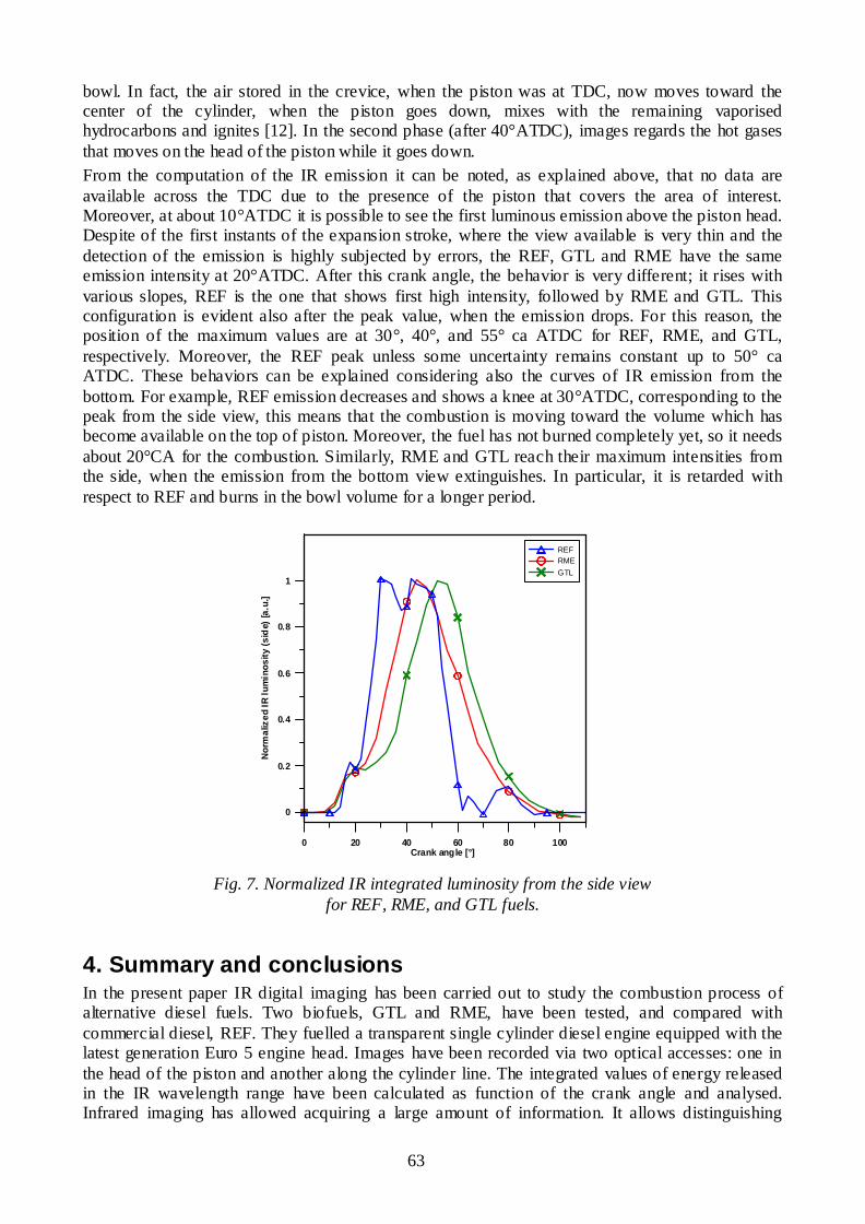
63

bowl. In fact, the air stored in the crevice, when the piston was at TDC, now moves toward the center of the cylinder, when the piston goes down, mixes with the remaining vaporised hydrocarbons and ignites [12]. In the second phase (after 40°ATDC), images regards the hot gases that moves on the head of the piston while it goes down. From the computation of the IR emission it can be noted, as explained above, that no data are available across the TDC due to the presence of the piston that covers the area of interest. Moreover, at about 10°ATDC it is possible to see the first luminous emission above the piston head. Despite of the first instants of the expansion stroke, where the view available is very thin and the detection of the emission is highly subjected by errors, the REF, GTL and RME have the same emission intensity at 20°ATDC. After this crank angle, the behavior is very different; it rises with various slopes, REF is the one that shows first high intensity, followed by RME and GTL. This configuration is evident also after the peak value, when the emission drops. For this reason, the position of the maximum values are at 30°, 40°, and 55° ca ATDC for REF, RME, and GTL, respectively. Moreover, the REF peak unless some uncertainty remains constant up to 50° ca ATDC. These behaviors can be explained considering also the curves of IR emission from the bottom. For example, REF emission decreases and shows a knee at 30°ATDC, corresponding to the peak from the side view, this means that the combustion is moving toward the volume which has become available on the top of piston. Moreover, the fuel has not burned completely yet, so it needs about 20°CA for the combustion. Similarly, RME and GTL reach their maximum intensities from the side, when the emission from the bottom view extinguishes. In particular, it is retarded with respect to REF and burns in the bowl volume for a longer period.

0 20 40 60 80 100Crank angle [°]

REFRMEGTL

0

0.2

0.4

0.6

0.8

1

Nor

mal

ized

IR lu

min

osity

(sid

e) [a

.u.]

Fig. 7. Normalized IR integrated luminosity from the side view for REF, RME, and GTL fuels.

4. Summary and conclusions In the present paper IR digital imaging has been carried out to study the combustion process of alternative diesel fuels. Two biofuels, GTL and RME, have been tested, and compared with commercial diesel, REF. They fuelled a transparent single cylinder diesel engine equipped with the latest generation Euro 5 engine head. Images have been recorded via two optical accesses: one in the head of the piston and another along the cylinder line. The integrated values of energy released in the IR wavelength range have been calculated as function of the crank angle and analysed. Infrared imaging has allowed acquiring a large amount of information. It allows distinguishing

64

chemical and/or physical activity of the injection and combustion process in advance or with more detail with respect to typical visible images. GTL emission starts before the energy released by the other fuels this is ascribed to the high value of its Cetane number. This means that the GTL has less time to premix it with the air in the bowl and thus realize more soot during the combustion. This is also in good agreement with the results of high PM emission and in-cylinder OH rates detected in previous papers. Moreover, the energy released on the top of the piston is the slowest than the other fuels, while it decreases quickly as the REF fuel. This is in good agreement with the fastest rate both for the formation and the oxidation of the soot. Probably, the GTL completes its combustion in the bowl and the unburned fuel and burned hot gases moves out the bowl slowly producing retarded IR energy detection. The GTL combustion behaviour entirely offset the benefit of fuel lack of aromatics. RME showed the most retarded start of combustion due to its LHV. Very low energy during the pilot combustion with respect to the other fuels has been detected. Moreover, the longest time for the autoignition, due to its lower Cetane Number, and the high oxygen content improved the RME mixing process providing a low soot combustion process. RME had the largest IR emission due to the highest energizing time of the main injection. Chemical activity is in progress up to 30° ATDC. Finally, the analysis of reactions occurring outside the piston bowl, shown RME flames have a propensity to migrate toward the volume which has become available on the top of the piston during the expansion stroke slower than REF and faster than GTL. The introduction of infrared technologies in the study of combustion engine functioning has revealed a good way to investigate the influence of alternative fuel in the combustion process especially when the visible imaging is not able to catch useful information. In particular, during the late combustion phase, the IR image showed a good capability to follow the hot burned gases both in the bowl and above the piston. Finally, the IR digital imaging of combustion process has revealed a tool with high potential

Acknowledgments The authors thank Mr. Carlo Rossi and Mr. Bruno Sgammato for their precious help.

Nomenclature ATDC After Top Dead Centre BTDC Before Top Dead Centre ca Crank Angle CCD Charge Coupled Device CR Common Rail DI Direct Injection ECU Electronic Control Unit EGR Exhaust Gas Recirculation ET Energizing Timing IR Infrared ROHR Rate Of Heat Release SOC Start Of Combustion SOI Start Of Injection TDC Top Dead Centre UV Ultraviolet VIS Visible VSA Variable Swirl Actuator

65

References [1] Assessment of barriers to the trade of biofuels between the European Union and Latin America

Prepared for BioTop project BioTop Deliverable 5.3 Project Nr 1412 Date April 2010 <http://www.btgworld.com/uploads/documents/Biofuel%20Trade%20Barriers%20BTG%20April%202010.pdf>

[2] McCormick, R. L., Alleman T. L., Fischer-Tropsch Diesel Fuels – Properties and Exhaust Emissions: A Literature Review. SAE Paper, 2003, 2003-01-0763.

[3] Peterson, C. L., Vegetable oil as a diesel fuel: Status and research priorities. Transactions of the ASAE 1986, 29(5), 1413-1422.

[4] Manca, D., Rovaglio, M., Infrared thermographic image processing for the operation and control of heterogeneous combustion chambers. Combustion and Flame, 2002 130, pp. 277-297.

[5] Founti, M., Kolaitis, D., Zannis, G., Kastner, O., Trimis, D., Experimental determination of fue l evaporation rates using IR-Thermography. QIRT 2002, 2002, Collegium Ragusinum, Dubrovnik, Croatia, September 24-27.

[6] Jansons, M., Lin, S., Fang, T., Rhee, K. T., Visualization of Preflame and Combustion Reactions in Engine Cylinders. SAE Paper, 2000, 2000-01-1800.

[7] Parker, T. E., Morency, J. R., Foutter, R. R., Rawlins, W. T., Infrared Measurements of Soot Formation in Diesel Sprays. Combustion and Flame, 1996, 107(3), 271–290.

[8] Chimenti, M., Di Natali, C., Mariotti, G., Paganini, E., Pieri, G., Salvetti, O., An IR image processing approach for characterising combustion instability. Infrared Physics & Technology, 2004, 46, 41–47.

[9] Mancaruso, E., Vaglieco, B. M., Premixed combustion of GTL and RME fuels in a single cylinder research engine. Applied Energy, 2012, 91, 385–394.

[10] Heywood, J. B., Internal Combustion Engine Fundamentals. McGraw-Hill, NewYork, 1988. [11] Mancaruso, E., Sequino, L., Vaglieco, B. M., IR Imaging of Premixed Combustion in a

Transparent Euro5 Diesel Engine. SAE Paper, 2011, 2011-24-0043. [12] Benajesa, J., Novella, R., García, A., Arthozoula, S., The role of in-cylinder gas density and

oxygen concentration on late spray mixing and soot oxidation processes. Energy, 2011, 36(3), 1599-1611.

PROCEEDINGS OF ECOS 2012 - THE 25TH INTERNATIONAL CONFERENCEON

EEEEFFICIENCY, CCCCOST, OOOOPTIMIZATION, SSSSIMULATION AND ENVIRONMENTAL IMPACT OF ENERGY SYSTEMS


66

Some aspects concerning fluid flow and turbulence modeling in 4-valve engines

Zoran Jovanovica, ZoranMasonicic

b, Miroljub Tomic

c

aInstitute “Vinca”, Head of Dept. for IC Engines, Univ. of Belgrade, [email protected] bInstitute “Vinca”, Dept. for IC Engines, Univ. of Belgrade, [email protected]

c Faculty of Mech. Engineering, Head of Dept. for IC Engines, Univ. of Belgrade, [email protected]

Abstract

In this paper some results concerning the structure and evolution of fluid flow pattern during induction and compression in 4-valve engines with tilted valves were presented. Results were obtained by dint of multidimensional modeling of non-reactive flows in arbitrary geometry with moving boundaries. During induction fluid flow pattern was characterized with organized tumble motion followed by small but clearly legible deterioration in the vicinity of BDC. During compression the fluid flow pattern is entirely three-dimensional and fully controlled by vortex motion located in the central part of the chamber. In order to annihilate negative effects of tumble deterioration and to enhance swirling motion one of the intake valves was deactivated. Some positive and negative effects of such attempt were elucidated. The effect of turbulence model variation was tackled as well. Namely, some results obtained with eddy-viscosity model i.e. standard k-ε model were compared with results obtained with k-ξ-f model of turbulence in domain of 4-valve engine in-cylinder flow. Some interesting results emerged rendering impetus for further quest in the near future. In the case of combustion all differences ensuing from turbulence model variation, encountered in the case of non-reactive flow were annihilated entirely. Namely the interplay between fluid flow pattern and flame propagation is invariant as regards both turbulence models applied.

Keywords:

Computational Fluid Dynamics (CFD), Automotive Flows, Turbulence Modelling

1. Introduction It is known for a long time that various types of organized flows in combustion chamber of IC

engines are of predominant importance for combustion particularly with regards to flame front

shape and its propagation. Some results related to the isolated or synergic effect of squish and swirl

on flame propagation in various combustion chamber layouts are already analysed and published [1,

2] but results concerning the isolated or combined effect of the third type of organized flow i.e.

tumble are relatively less presented and sometimes ambiguous [3, 4]. For instance some authors [5]

studied the development of swirl and tumble in five different intake valve configurations and found

that when both inlet valves are opened no defined tumble flow structure was created rendering

quick vortices dissipation before BDC. In spite of the fact that tumble flow is inherent to multi-

valve engines some authors have demonstrated that some two-valve engines exhibit characteristics

similar to tumble flow [6, 7]. In addition, the fairly similar fluid flow patterns in the vicinity of

BDC in various combustion chamber geometries yield entirely different fluid flow patterns, spatial

distribution of kinetic energy of turbulence and integral length scales of turbulence in the vicinity of

TDC [8]. In such occasions the significance of organized tumble flow is fairly relative. Some

theoretical and experimental results show that tumble is of prime importance for specific power and

fuel economy increase in modern engines with multi-valve systems. The beneficial effects of

tumble on CO, CH and NOx were also demonstrated. From the theory of turbulence is known that

vortex filament subjected to compression reduces its length and promotes rotation around its axis

yielding the movement on the larger scale (“spin-up” effect). It can be presumed that tumble

67

pursues the same rule i.e. the destruction of formed and expressive tumble during compression

stroke generates the higher turbulence intensity and larger integral length scale of turbulence in the

vicinity of TDC contributing to the flame kernel formation period reduction and faster flame

propagation thereafter. The aforementioned logic imposes the conclusion that the most beneficial

fluid flow pattern in the vicinity of BDC is well shaped high intensity tumble. Some additional

objectives in this paper were qualitative and quantitative characterization of fluid flow pattern

during induction and compression in a particular 4-valve engine, the analysis of the valve/port

assembly from the point of compliance with presumed ideal fluid flow pattern, the effect of port deactivation and the clout of turbulence model variation on fluid flow and turbulence parameters.

2. Model and computational method The analysis of this type is inherent to multidimensional numerical modelling of non-reactive fluid

flow and therefore it is quite logical to apply such a technique particularly due to fact that it is the

only technique that encompasses the valve/port geometry layout in an explicit manner. In lieu of the

fact that, in its essence, multidimensional models require initial and boundary conditions only their

applications is fairly complicated and imply some assumptions and simplifications [9]. The full 3D

conservation integral form of unsteady equations governing turbulent motion of non-reactive

mixture of ideal gas is solved on fine computational grid with moving boundaries (piston and

valves) in physical domain (66.000-682.000 cells) by dint of two different codes. The first one is

KIVA 3V release 2 code running on UNIX Ultra SUN II computer [10, 11, 12, 13]. This code is

used in the first part of this paper in order to scrutinize clouts of intake port geometry variations on

in-cylinder fluid flow. The second code used is well known AVL FIRE 2009.1 code [14] used to

investigate the effect of turbulence model variations on fluid flow and flame propagation. In both

cases the numerical solution method is based on a fully conservative finite volume approach (CGR

method). All dependent variables such as momentum, pressure, density, turbulence kinetic energy,

dissipation rate, and passive scalar are evaluated at the cell centre. A second-order midpoint rule is

used for integral approximation and a second order linear approximation for any value at the cell-

face. A diffusion term is incorporated into the surface integral source after employment of the

special interpolation practice. The convection is solved by a variety of differencing schemes

(upwind or donor cell, interpolated donor cell, quasi second order differencing, central differencing,

MINMOD and SMART). The rate of change is differenced by using implicit schemes i.e. Euler

implicit scheme and three time level implicit scheme of second order accuracy. The overall solution

procedure is iterative and is based on the Semi-Implicit Method for Pressure-Linked Equations

algorithm (SIMPLE). For the solution of a linear system of equations, a conjugate gradient type of

solver (CGS) is used. Two different models of turbulence were used. The first one is nearly forty

years old k-ε model based on Boussinesq’s assumption which is certainly the most widely used

model for engineering computations. On the contrary to some other models, such as Reynolds-stress

closure model [15], its implementation is numerically robust due to simplicity of the model and at

the same provides an acceptable level of accuracy for particular applications. The second one is

relatively recent k-ξ-f model of turbulence i.e. eddy-viscosity model based on Durbin’s elliptic

relaxation concept [16, 17]. This model solves a transport equation for the velocity scale ratio ξ

instead of imaginary turbulent normal stress component. In addition, the pertinent hybrid boundary

conditions were applied. The combustion model implemented is well known Eddy Breakup model.

This model implies the assumption that reactants are in the same eddies and are clearly separated

from eddies that contain hot combustion products. Due to the fact that chemical reactions have time

scale very short in comparison to the characteristics of turbulent transport processes it can be

assumed that the rate of combustion is determined by the rate of intermixing on a molecular scale of

the eddies reactants and those containing hot products. The major feature of this model is the fact that it does not call for predictions of fluctuations of reacting species.

68

3. Results and discussion The analysis of fluid flow pattern during induction and compression was based on a fairly

complicated geometry layout presented in figs.1.and2. Obviously, combustion chamber is

constrained with dual intake and exhaust valves. In spite of the fact that it is not of crucial

importance the inclination of intake and exhaust port is 200 and 22

0 respectively. The basic block

data sheet consists of bore/stroke ratio = 9.2/8.5 cm, inlet valve head diameter = 3.65 cm, exhaust

valve diameter = 3.25 cm, squish gap = 0.115 cm, engine speed RPM = 2500 min-1

and mixture

quality λ=1. It should be stated that maximum valve lift is Li=0.962 cm while the other geometrical

data (relative location, valve shape etc.) could be seen in fig.1 and 2. In the case with simultaneous

valve opening the commencement of intake valves opening was set at 150 BTDC and their closure

at 1950 ATDC.

Fig.1: Perspective view of the combustion chamber geometry layout with 4-valves (upper

view)

Fig.2: Perspective view of the combustion chamber geometry layout with 4-valves (bottom view)

The results presented in figures 3-27 are obtained with KIVA 3V release 2 code and k-ε model of

turbulence, while the rest are obtained with the AVL FIRE 2009.1 code and two different

turbulence models (k-ε and k-ξ-f). The evolution of fluid flow pattern and turbulence was pursued

in five cut-planes (in x-z plane, y=2.1 cm, passing through one intake and one exhaust valve, in

symmetry x-z plane, y=0, in y-z plane, x=-2.1 cm, passing through both intake valves, in y-z plane,

x=2.1 cm, passing through both exhaust valves and in x-y plane at z=8.6 cm). The evolution of fluid

flow pattern, represented as vectors, in vertical x-z plane (y=2.1 cm or y=-2.1cm for simultaneous

valve opening) is shown in fig. 3, 4 and 5. As can be seen in fig.3 high velocity intake jet flows over

the valve, strikes upon the piston crown, curls and commences to form an elliptically-shaped vortex

around y-axis in counter-clockwise direction, provided that it is stipulated as such, on the left side

of the valve. A small tumble-like vortex motion is created by the intake jet in clockwise direction to the right of the valve (fig.3).

69

Fig.3: Fluid flow pattern in x-z plane, y=2.1cm, at 600 ATDC, k-ε

At 600

ATDC these two vortices are of the same intensity (fig.3) indicating the zone of coinciding

flow followed by separation region just beneath the intake valve face. These two vortices are part of

thoroidalring vortex that can be verified in fig. 6.

Fig.4: Fluid flow pattern in x-z plane, y=2.1 cm, at 1200 ATDC, k-ε

Fig.5: Fluid flow pattern in x-z plane, y=2.1 cm, at 1700 ATDC, k-ε

Fig.6: Fluid flow pattern in y-z plane, x=-2.1cm, at 300 ATDC, k-ε

Namely, the centre of rotation is equally distributed around the perimeter beneath the valve face.

The increase of tumble motion intensity at maximum valve lift and further movement of piston

downward exerts the attenuation of the vortex flow on the left side of intake valve. Obviously, the

vortex flow is squeezed out and its shape becomes elongated (along z-axis). It’s interesting to note

that the centre of rotation of tumble motion is in the same position. The formed tumble flow around

y-axis reduces the activity of that vortex to the zone in the vicinity of cylinder wall particularly

from the moment when valve movement changes its direction (fig.4). In the vicinity of BDC the

direction of vortex flow is changed due to tumble motion and its role reduced entirely to the close

proximity of intake valve face (fig.5). In addition, the centre of rotation of tumble motion is slowly

displaced to the right side of cylinder wall Such a movement is followed by new vortex formation

in the corner located adjacent to the bottom right side indicating the subtle deterioration of general

tumble motion. Non-uniform distribution of tumble intensity along y-axis and two symmetric

vortices in x-y plane in the vicinity of cylinder wall are responsible for the deterioration of tumble

flow near BDC. Namely, as can be seen in fig.7 the tumble intensity in vertical plane for y=0 is

more expressive than tumble intensity for y=± 2.1 cm. No deterioration of tumble motion in vertical

plane for y=0 is encountered. In addition, larger velocities are encountered in the central part of the

chamber ensuing partly from jet penetration from the flanks. This activity is enhanced by vortices in

70

x-y plane which prevent the tumble motion in vertical plane (y=± 2.1) to reach the cylinder wall.

The net result is the deflection of fluid flow in y-z plane (x=2.1 cm) along z-axis and formation of symmetric vortices adjacent to piston crown (fig.8).

Fig.7: Fluid flow pattern in x-z plane, y=0 cm, at 1500 ATDC, k-ε

Fig.8: Fluid flow pattern in y-z plane, x=2.1 cm, at 1750 ATDC, k-ε

The formation of tumble motion is observed as well through evolution of fluid flow pattern in x-

y plane, as shown in fig. 9 and 10.

Fig.9: Fluid flow pattern in x-y plane, z=8.6 cm, at 600 ATDC, k-ε


A symmetric flow structure is created about the plane of symmetry of the cylinder head, y=0, even

though no conditions of symmetry were applied to the flow. It should be noted that variable visible

segments of valves are due to valve movement. As can be seen in fig. 9 the synergic action of the

flows over the two intake valves generates a jet travelling across the cylinder away from intake

valves, formed approximately in the midway from the cylinder centre to the right wall. Two

counter-rotating vortices are observed on the very left side of the cylinder. Regions of low velocity

magnitude are identifiable on the very right of the cylinder indicating large velocity component in

z-direction. Annihilating effect of the combination of the flow is evident in the upper part of the

71

symmetry plane (fig.7). As can be seen in fig.10 two counter rotating vortices are clearly legible on

the very right side of the cylinder as well. The entire region is engulfed with counter rotating vortex

motion in the vicinity of BDC. Namely the curling of the flow is obvious in the central part as well

indicating the ingress of the fluid flow from the flank followed by deterioration of tumble motion.

During compression, the quick decay of vortex motion in the zone beneath intake valves and in the

vicinity of piston crown is encountered. Further movement of piston upwards yields the restitution

of organized vortex motion with its centre of rotation around x=0. The fairly expressive w-

component of the velocity in the zone of intake valves is observed rendering 1D fluid flow

thereafter. In x-z plane, z=8.61 cm, on the very beginning of compression the intensive flank flows

exerts detention of strong coinciding flow along x-axis, y=0, and changes its direction to intake

valves.



High intensity coinciding flow in x-y plane is fairly similar to the fluid flow pattern in x-y plane

during induction but in opposite direction (fig. 11 and 12)

Fig.13 Spatial distr. of kinetic energy of turbulence in x-z plane, y=-2.1 cm, at 3450 ATDC, k-ε

Non-uniformity of fluid flow pattern along y-axis is followed by non-uniform spatial distribution of

kinetic energy of turbulence along y-axis. Namely, in x-z plane, y=-2.1 cm, the zone with relatively

high kinetic energy of turbulence is spread out through the entire region (fig.13) while in symmetry

plane, y=0, the zone with high kinetic energy of turbulence is, due to strong coinciding flow (u-component dominant flow) squeezed to the zone between cylinder wall and intake valves (fig.14).

72

Fig.14: Spatial distribution of kinetic energy of turbulence in x-z plane, y=0, at 3450 ATDC

Such a non-uniformity along y-axis yields characteristic and fairly inconvenient “bean-like” shape

of spatial distribution of kinetic energy of turbulence in x-y plane, as can be seen in fig.15.

Fig.15: Spatial distribution of kinetic energy of turbulence in x-y plane, z=8.6 cm, at 3450 ATDC

In order to prevent strong coinciding flow along x-axis yielding inconvenient spatial distribution of

kinetic energy of turbulence in the vicinity of TDC port deactivation was included in analysis as

well. The rationale for such a step is the presumption of fairly convenient mutual interaction

between tumble and swirl, not observed in the case with simultaneous valve openings that could

contribute to the better spatial distribution of kinetic energy of turbulence in the vicinity of TDC.

Fig.16: Fluid flow pattern in y-z plane, x=-2.1 cm, at 600 ATDC, port deactivation, k-ε

As can be seen in fig.16 port deactivation means that one of the intake valves is kept closed and as a

consequence the fluid flow pattern is entirely asymmetric. The evolution of the fluid flow in the cut-plane passing through one active and one exhaust valve is shown in fig.17 and 18.

Fig.17: Fluid flow pattern in x-z plane, y=2.1 cm, at 600 ATDC, port deactivation, k-ε

73

Fig.18: Fluid flow pattern in x-z plane, y=2.1 cm, at 1700 ATDC, port deactivation, k-ε

Fig.19: Fluid flow pattern in x-z plane, y=0, at 1200 ATDC, port deactivation, k-ε


At the very beginning of induction the fluid flow pattern is fairly similar to the previous case

(fig.17). Namely, two counter rotating vortices around y-axis are observed as well. On the contrary

to the case with both intake valves opened there is no constraint imposed by fluid flow through

another intake valve and therefore no squeezing out of vortex motion in the intake valve zone is

encountered. The majority of the fluid flow is directed astray and promotes vortex motions around

y-axis in a set of parallel x-z planes (fig. 18 and 19). The flank flows from the zone with active

intake valve promotes the formation of two concentric vortex flows around y-axis in symmetry

plane, y=0 (fig.19). The intensity of the inner vortex prevails and its axis of rotation gradually

moves to the central part of the chamber (fig.20) and persists there up to the end of compression

stroke (fig.21).


The evolution of the fluid flow pattern in x-z cut plane passing through inactive intake valve is

shown in fig.22 and 23.

74

Fig.22: Fluid flow pattern in x-z plane, y=-2.1 cm, at 600 ATDC, port deactivation, k-ε

Fig.23: Fluid flow pattern in x-z plane, y=-2.1 cm, at 1700 ATDC, port deactivation, k-ε

Large soothing zones in fig.22 indicate strong v-component velocities. In the vicinity of BDC

formed vortex motion around y-axis, similar to that in symmetry plane, y=0, is observed as well

(fig.23).

Fig.24: Fluid flow pattern in x-y plane, z=8.6 cm, at 1700 ATDC, port deactivation, k-ε

It's interesting to note that the entire zone of inactive intake valve is engulfed with large-scale

vortex motion. In addition to the vortex motion around y-axis, strong vortex motion around z-axis,

in the vicinity of BDC, is encountered as well (fig.24) being transformed, due to its increased intensity, into formed swirling flow in the vicinity of TDC thereafter (fig.25).

Fig.25: Fluid flow pattern in x-y plane, z=8.6 cm, at 3450 ATDC, port deactivation k-ε

The spatial distribution of kinetic energy of turbulence replicates entirely the fluid flow pattern and

is shown in fig.26 and 27.

75

Fig.26: Spatial distribution of kinetic energy of turbulence in x-z plane, y=0, at 3450 ATDC, port

deactivation, k-ε

Fig.27: Spatial distribution of kinetic energy of turbulence in x-y plane, z=8.6 cm, at 3450 ATDC,

port deactivation, k-ε

As can be seen in fig.26 and 27 the spatial distribution of kinetic energy of turbulence is more

convenient than in the case with simultaneous intake valve opening. Namely, regularly shaped zone

of high kinetic energy of turbulence is located in the central part of the chamber and occupies the

entire region along z-axis between piston crown and cylinder head. The effects of turbulence model

variation on the evolution of fluid flow pattern and spatial distribution of kinetic energy of

turbulence in 4.-valve engine were presented in figs.28-39 below. Namely, figs. 28, 31, 34 and 37

are related to standard k-ε model of turbulence while figs. 29, 32, 35 and 38 are related to k-ξ-f

model of turbulence. Due to symmetry in x-y plane results for both model of turbulence were

presented in the same figure (figs. 30, 33, 36 and 39). In order to alleviate comparisons of fluid flow

patterns particularly in the case of subtle differences colours were employed as well.

Fig.28: Fluid flow pattern in x-z plane, y=const.at 340 deg. ATDC, k-ε

Fig.29: Fluid flow pattern in x-z plane, y=const.at 340 deg. ATDC, k-ξ-f

During induction and large portion of compression stroke (up to 270 deg. ATDC) no legible

differences as regards the evolution of fluid flow pattern and spatial distribution of kinetic energy of

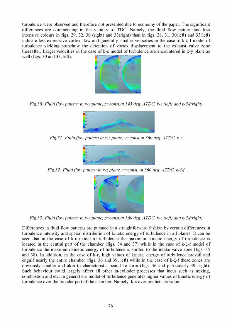
76

turbulence were observed and therefore not presented due to economy of the paper. The significant

differences are commencing in the vicinity of TDC. Namely, the fluid flow pattern and less

intensive colours in figs. 29, 32, 30 (right) and 33(right) than in figs. 28, 31, 30(left) and 33(left)

indicate less expressive vortex flow and generally smaller velocities in the case of k-ξ-f model of

turbulence yielding somehow the detention of vortex displacement to the exhaust valve zone

thereafter. Larger velocities in the case of k-ε model of turbulence are encountered in x-y plane as well (figs. 30 and 33, left).

Fig.30: Fluid flow pattern in x-y plane, z=const.at 345 deg. ATDC, k-ε (left) and k-ξ-f(right)

Fig.31: Fluid flow pattern in x-z plane, y=const.at 360 deg. ATDC, k-ε

Fig.32: Fluid flow pattern in x-z plane, y=const. at 360 deg. ATDC, k-ξ-f

Fig.33: Fluid flow pattern in x-y plane, z=const.at 360 deg. ATDC, k-ε (left) and k-ξ-f(right)

Differences in fluid flow patterns are pursued in a straightforward fashion by certain differences in

turbulence intensity and spatial distribution of kinetic energy of turbulence in all planes. It can be

seen that in the case of k-ε model of turbulence the maximum kinetic energy of turbulence is

located in the central part of the chamber (figs. 34 and 37) while in the case of k-ξ-f model of

turbulence the maximum kinetic energy of turbulence is shifted to the intake valve zone (figs. 35

and 38). In addition, in the case of k-ε, high values of kinetic energy of turbulence prevail and

engulf nearly the entire chamber (figs. 36 and 39, left) while in the case of k-ξ-f these zones are

obviously smaller and akin to characteristic bean-like form (figs. 36 and particularly 39, right).

Such behaviour could largely affect all other in-cylinder processes that incur such as mixing,

combustion and etc. In general k-ε model of turbulence generates higher values of kinetic energy of turbulence over the broader part of the chamber. Namely, k-ε over predicts its value.

77

Fig.34: Spatial distribution of kinetic energy of turbulence in x-z plane, y=const. at 340 deg. ATDC,

k-ε


k-ξ-f

Fig.36: Spatial distribution of kinetic energy of turbulence in x-y plane, z=const. at 340 deg. ATDC,

k-ε (left) and k-ξ-f(right)


k-ε


k-ξ-f

Fig.39: Spatial distribution of kinetic energy of turbulence in x-y plane, z=const. at 360 deg. ATDC,

k-ε (left) and k-ξ-f(right)

The fairly interesting results were obtained in the case of combustion that was tackled as well.

Namely, combustion was modelled in an eclectic, worldwide theoretically and experimentally

78

validated way [9]. In the case of combustion all the subtleties as regards fluid flow pattern and

spatial distribution of kinetic energy of turbulence due to turbulence model alteration, observed in

figs. 28-39, were annihilated entirely. The fluid flow pattern and flame propagation (represented as

iso-contours of temperatures) in various cut planes, for two different models of turbulence (k-ε and k-ξ-f) were presented in figs. 40-47, below.

Fig.40: Fluid flow pattern in x-z plane, y=const. (0.0) at 355 deg. ATDC, k-ε

Fig.41: Fluid flow pattern in x-z plane, y=const. (0.0) at 355 deg. ATDC, k-ξ-f

Fig.42: Spatial distribution of temperature in x-z plane, y=const. (0.0) at 355 deg. ATDC, k-ε

Fig.43: Spatial distribution of temperature kinetic in x-z plane, y=const. (0.0) at 355 deg. ATDC, k-

ξ-f

Fig.44: Fluid flow pattern in x-y plane, z=const. (mid-height of the wedge chamber) at 355 deg.

ATDC, k-ε (left) and k-ξ-f (right)

Fig.45: Spatial distribution of temperature in x-y plane, z=const. (mid-height of the wedge

chamber) at 355 deg. ATDC, k-ε (left) and k-ξ-f (right)

79

Fig.46: Fluid flow pattern in x-y plane, z=const. (squish zone) at 355 deg. ATDC, k-ε (left) and k-ξ-f

(right)

Fig.47: Spatial distribution of temperature in x-y plane, z=const. (squish zone) at 355 deg. ATDC,

k-ε (left) and k-ξ-f (right)

It can be seen, in figs. 40, 41, 44 and 46 that, in the case of combustion, no clear difference in fluid

flow pattern is observed. Namely, the well-known “flame dominated fluid flow pattern” is

encountered characterized with higher velocities in front of the flame front and relaminarization

behind the flame front (figs. 40, 41, 44 and 46). This is legible in all cut planes considered. In

comparison with corresponding fluid flow pattern in no combustion case (figs. 31, 32 and 33) clear

differences are indicated. The main reason for the relaminarization of the fluid flow behind the

flame front lies in the fact that flame propagation through un-burnt mixture, entire of itself,

accelerates the hot gas in front of the flame front. In the case of shear the production of turbulence

increases with the effect of flame acceleration thereafter. In the compressed zone in front of the

flame front the divergence of the mean velocity is negative yielding the generation of turbulence as

well. In addition the sign and the magnitude of the density gradient within the flame affect the

diffusion of turbulence. Referring to the energy conservation equation one can find the maximum

enthalpy in the zone of minimal density, i.e. behind the flame front so these higher temperatures

cause the intensive increase of viscosity with the consequential increase of Ret-number, the increase

of viscous dissipation of turbulence and shifting of the velocity fluctuations to the low frequency

part of spectrum. In the heat release zone the dilatation of turbulence reduces the turbulent kinetic

energy yielding fairly legible soothing or attenuation (relaminarization) of the fluid flow. It can be

seen, in figs. 42, 43, 45 and 47, that in a particular combustion chamber geometry layout, flame

propagation as regards its velocity and its flame front shape is entirely invariant vis-à-vis alteration

of k-εmodel of turbulence to k-ξ-f model of turbulence.

4. Conclusions The fluid flow pattern during induction and compression in the particular combustion chamber

geometry of 4-valve engine is extremely complex and entirely three-dimensional. In the case with

two valves opened tumble motion during induction is clearly legible and followed by gradual

deterioration in the vicinity of BDC due to non-uniform distribution along y-axis. During

compression strong vortex flow around y-axis and fairly expressive coinciding flow along x-axis in

reverse direction is encountered contributing to the inconvenient spatial distribution of kinetic

energy of turbulence in the vicinity of TDC. Some benefits concerning generation of swirling flow

and better spatial distribution of kinetic energy of turbulence in the vicinity of TDC were gained

with port deactivation. The modelling of turbulence strongly affects the evolution of fluid flow

pattern and spatial distribution of kinetic energy of turbulence in 4-valve engines. In general k-ε

model of turbulence generates higher values of kinetic energy of turbulence over the broader part of

80

the chamber than corresponding k-ξ-f model of turbulence. In the case of combustion all differences

ensuing from turbulence model variation, encountered in the case of non-reactive fluid flow were

annihilated entirely. This is verified elsewhere [18] particularly when Reynolds stress closure is

excluded. This occurs in the case of so called “flame dominated fluid flow”, where the situation

before combustion has slight effect on the flame propagation ahead. This is only one of three

possible cases of macro flows that can be encountered in IC engines. In the case of other two types

of macro flows i.e. “squish dominated” and “coincident” flows respectively, the situation before

combustion has a major effect on flame propagation [2]. Namely, in the case of squish dominated

flow the radial component is responsible for flame propagation while in the case of coincident flow

there is a balance between squish (macro flows) and turbulence intensity generated by the flame.

5. References [1] J. Danneman, K. Pielhop, M. Klaas, W. Schroeder(2010) „Cycle resolved multi planar flow

measurements in a four valve combustion engine”, Exp.Fluids, Research article, DOI 10.1007/s00348-010-0963-4

[2] Z. Jovanovic, S. Petrovic “The mutual interaction between squish and swirl in IC Engines“,

(1997) Mobility and Vehicle Mechanics 23, 3, 72-86

[3] K. Lee, C. Bae, K. Kang “The effects of tumble and swirl flows on flame propagation in a four-valve S.I.engine”, Applied Thermal Engineering 27 (2007) 2122-2130

[4] G.J.Micklow, W. D. Gong “Intake and in cylinder flow field modeling of a four valve diesel

engine” Proc.IMechE(2007) vol. 221, Journal of Automobile Engineering, 1425-1440

[5] B. Khaligi “Intake generated swirl and tumble motion in a 4.-valve engine with various intake configurations“ SAE Paper 900059

[6] Z.Jovanovic, S. Petrovic, M. Tomic “The effect of combustion chamber geometry layout on

combustion and emission” (2008) Thermal Science vol.12, No.1, pp. 7-24

[7] Z. Jovanovic, Z.Masonicic, M. Tomic „The vice-verse movement of the reverse tumble centre

of rotation in a particular combustion chamber“, MTM Machines Technologies Materials, Year

II, issue 6-7, (2008) ISSN 1313-0226l, pp. 17-20

[8] Z. Masonicic, Z. Jovanovic “The effect of combustion chamber geometry layout variations

onto fluid flow pattern“, International Automotive Conference with Exhibition, SCIENCE

AND MOTOR VEHICLES, NMV0774, Belgrade, 2007, ISBN 978-86-80941-31-8

[9] Z.Jovanovic “The role of tensor calculus in numerical modeling of combustion in IC engines”

Computer Simulation in Fluid Flow, Heat and Mass Transfer and Combustion in Reciprocating

Engines, Hemisphere Publishers (1989) 457-542, ISBN 0-89116-392-1

[10] A. A. Amsden, KIVAII: Acomp. prog. for reactive flows with sprays,LA-11560-MS,1989

[11] A. A. Amsden, KIVA3V, Rel.2 Improvements to KIVA3V, LA-UR-99-915, 1999

[12] A. A. Amsden, SALE3D: A simplified ALE computer program for calculating 3D fluid flows, NUREG-CR-2185, 1982, 11560-MS, 1989

[13] D. J. Torres, M. F. Trujillo, KIVA-4: An unstructured ALE code for compressible gas flow

with sprays, Journal of Computational Physics, 219 (2006), pp.943-975

[14] CFD Solver, AVL FIRE 2009.1

[15] C.G. Speciale, S. Sarkar, T. B. Gatski „Modelling the pressure strain correlation of turbulence – an invariant dynamical system approach“, pp.1-51, ICASE Report No. 90-5, 1990

[16] K.Hanjalic, M.Popovac, M.Hadjiabdic „A robust near-wall elliptic relaxation eddy viscosity

turbulence model for CFD”, International Journal of Heat and Fluid Flow, 25(2004) 1047-1051

[17] P.A.Durbin „Near wall turbulence closure modeling without damping functions“,Theor.Comput. Fluid Dynamics (1991) 3 1-13

81

[18] B. Basara, Z. Jovanović: "The current capabilities of turbulence modeling in Automotive

Flows“ YUMV 010021, pp. 93-96, Beograd , 2001



82

Adapting the operation regimes of trigeneration systems to the renewable energy systems integration

Liviu Ruieneanua and Mihai Paul Mirceab a University of Craiova, Craiova, Romania, [email protected]

b University of Craiova, Craiova, Romania, [email protected]

Abstract: The purpose of the paper is to evaluate the potential for parallel operation of conventional CHP/trigeneration plants and wind turbines. This approach allows the identification of the best possible operation scenarios for the conventional plants in order to contribute to a fast integration of the wind turbines into the energy production mix. The mathematical model presented in the paper allows the determination of a safe operation domain where the power variations of the wind turbines are fully compensated by the conventional plant for different operation regimes. The results also reveal the necessity of a differentiated CO2 emissions tax calculated at system level and not at the level of the conventional power plants. This is important because sometimes increased CO2 emissions of the conventional power plants might lead to an overall decrease of the CO2 emissions at system level (for example when conventional plants are operating at partial loads in order to allow an increased electricity production of the wind turbines).

Keywords: Trigeneration, District heating/cooling.

1. Introduction In Romania the installed power of the wind turbines was at the end of 2011 around 500 MW. By the end of 2012 the installed power will increase rapidly due to new subsidies for renewable sources. Even if Romania has a high number of hydro power plants (covering 30% of the total demand), the stability of the national grid is often ensured by conventional power plants with steam turbines. The main reason for that resides in the high price of the electrical energy sold by these plants. By maintaining the stability of the system these power plants receive a higher price for the electrical energy, remaining competitive. However reserving this role for conventional power plants is somehow complicated because these plants were designed for base loads. The problem becomes acute when power plants on coal are operating in parallel with wind turbines due to the coal power plants high inertia. In this paper we are trying to evaluate the cogeneration and trigeneration potential to increase the flexibility in power supply of these plants.

2. Indicators used for the analysis In order to analyse the implications of an important role for the renewable sources on the energy market we have considered a complex system consisting of a trigeneration plant and a wind farm. The purpose of the mathematical model is the calculation of the electrical energy that might be produced by the wind turbines within this complex system without an exchange of energy outside the system borders. In other words the power supply of the trigeneration plant has to be flexible enough to compensate the power variations of the wind turbines.

83

Fig. 1. The scheme of the analysed system

In order to evaluate the best solution for the trigeneration plant we have considered both absorption and compressor chillers. For the purpose of the analysis, both types of chillers have to be able to supply the entire cooling demand of the consumers. In order to analyse the influence of the wind turbines operation over the trigeneration we have used the trigeneration plants efficiency relation proposed in [8], particularized for the scheme presented in figure 1:

epbepcg

AbCCmpCAbCpkcgCmpCcgtr QQ

CCQQQEE (1)

When there is no cooling demand, the trigeneration efficiency becomes the total efficiency of the CHP plant [13]. In fact by grouping different terms this becomes obvious:

epbepcg

CmpCCmpC

epbepcg

AbCAbCtcgtr QQ

COPEQQ

COPQ )1()1( (2)

In a similar way it might also be defined an equivalent efficiency for the entire system depicted in figure 1 (trigeneration plant plus wind farm) as follows:

epbepcgtr

epbepcgtr QQ

EwQQ

CsQsEs (3)

In order to highlight the integration of the wind turbines all the calculation were made in relation with the quota of the electricity produced by the wind turbines:

s

ww E

Ef (4)

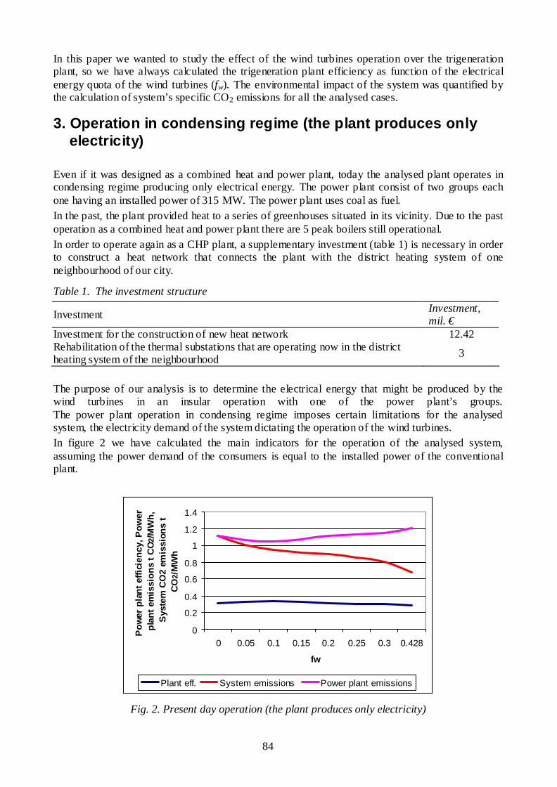
84

In this paper we wanted to study the effect of the wind turbines operation over the trigeneration plant, so we have always calculated the trigeneration plant efficiency as function of the electrical energy quota of the wind turbines (fw). The environmental impact of the system was quantified by the calculation of system’s specific CO2 emissions for all the analysed cases.

3. Operation in condensing regime (the plant produces only electricity)

Even if it was designed as a combined heat and power plant, today the analysed plant operates in condensing regime producing only electrical energy. The power plant consist of two groups each one having an installed power of 315 MW. The power plant uses coal as fuel. In the past, the plant provided heat to a series of greenhouses situated in its vicinity. Due to the past operation as a combined heat and power plant there are 5 peak boilers still operational. In order to operate again as a CHP plant, a supplementary investment (table 1) is necessary in order to construct a heat network that connects the plant with the district heating system of one neighbourhood of our city.

Table 1. The investment structure

Investment Investment, mil. €

Investment for the construction of new heat network 12.42 Rehabilitation of the thermal substations that are operating now in the district heating system of the neighbourhood 3

The purpose of our analysis is to determine the electrical energy that might be produced by the wind turbines in an insular operation with one of the power plant’s groups. The power plant operation in condensing regime imposes certain limitations for the analysed system, the electricity demand of the system dictating the operation of the wind turbines. In figure 2 we have calculated the main indicators for the operation of the analysed system, assuming the power demand of the consumers is equal to the installed power of the conventional plant.

0

0.2

0.4

0.6

0.8

1

1.2

1.4

0 0.05 0.1 0.15 0.2 0.25 0.3 0.428

fw

Pow

er p

lant

effi

cien

cy, P

ower

pl

ant e

mis

sion

s t C

O2/

MW

h,

Sys

tem

CO

2 em

issi

ons

t C

O2/

MW

h

Plant eff. System emissions Power plant emissions

Fig. 2. Present day operation (the plant produces only electricity)

85

The graph shows that the maximum power quota of the wind turbines (fw=0.42) is conditioned by the minimum operational power of the conventional power plant’s group (180 MW). The quota of the wind turbines power will decrease with the overall power demand of the system. The graph shows that the integration of the wind turbines is decreasing the system’s CO2 emissions. So, even if partial load operation of the conventional plant decreases it’s efficiency and that leads to an increase of the power plant’s CO2 emissions; the overall emissions for the entire system are decreasing (obvious if we compare the orange and the pink line). This effect imposes the introduction of a differentiated CO2 tax so that the conventional plants that are operating at partial loads for the integration of the wind turbines will not to be further affected by an increase of the CO2 emissions tax. The operation in domain of the system was dictated by the minimum operation limit in condensing regime of the conventional plant (table 2).

Table 2. Operation domains for the condensing operation regime Domain MW System operation domain 180-450 Safe operation domain 180 - 315

4. Operation in cogeneration regime The link between the generated power and the heat output for the steam extraction turbines, might be used to increase the flexibility of the power supply of the conventional power plants. The condition is the use of oversized peak boilers that might provide the entire heat demand of the consumers (not only the peak load). This practice is common to many combined heat and plants designs so that these plants could provide heat to the consumers when a malfunction occurs. By increasing the quota of the heat produced by the peak boilers or by using exclusively it’s peak boilers, the plant increases it’s power by shifting from cogeneration to separate production of electricity and heat.

0

0.1

0.2

0.3

0.4

0.5

0.6

0.7

0.8

0.9

1

0.42857 0.45714 0.48571 0.51429 0.54286 0.57143 0.57937

fw

CHP

pla

nt to

tal e

ffici

ency

90% Peak boilers eff.80% Peak boilers eff.70% Peak boilers eff.

Fig. 3. CHP plant efficiency variation for different peak boilers efficiency (when compensating a wind farm power drop)

86

Figure 3 depicts the behaviour of the system for a 100% heat demand (319.6 MW). By shifting from cogeneration to separate production the power of the conventional plant decreases with the increase of the power injected by the wind turbines. The use of peak boilers operating with high efficiencies improves the global efficiency of the system (figure 3). In figure 4, for a 100% heat demand the power of the wind turbines might get close to 58 % of the total power injected by the system. The method is very effective because the cogeneration plant might compensate any decrease of the wind turbines power in the safe operation domain. The downside of the method is the decrease of the global efficiency with the shift to separate production. The lower operation point of the system drops to a power of 132.5 MW (table 3) from 180 MW in condensing regime (table 2). Therefore by supplying heat in cogeneration the conventional power plant has a better power supply flexibility, thus increasing the reserve of the system for parallel operation with the wind farm.

Table 3. Operation domains for 100% heat demand Domain MW System operation domain 132.5-500 Safe operation domain 132.5 - 315 If the total electricity demand of the consumers decreases, than the power injected by the wind turbines has to decrease since the conventional plant produces the technological minimum power (132.5 MW).

00.10.20.30.40.50.60.70.80.9

1

0.43 0.46 0.49 0.51 0.54 0.57 0.58

fw

CHP

pla

nt e

ffici

ency

, CO

2 em

issi

ons

90% Peak boilers eff.t CO2/MWh

Fig. 4. Compensating a wind farm power drop in cogeneration operation regime at 100% heat demand

The decrease of the heat demand limits the CHP plant ability to compensate sudden drops of wind turbines power and leads to an increase of the CO2 emissions of the system.

87

Figure 5 depicts the system’s behaviour at 50 % heat demand.

0

0.1

0.2

0.3

0.4

0.5

0.6

0.7

0.42857143 0.45714286 0.48571429 0.50285714

fw

CHP

plan

t eff.

, CO

2 em

issi

ons

CHP eff.tCO2/MWh

Fig. 5. Compensating a wind farm power drop in cogeneration operation regime at 50% heat demand

Figure 5 shows that even in the worst case, when the efficiency of the CHP plant drops to nearly 40 % (separate production of electricity and heat) because the plant has to compensate power drop of the wind turbines, the CO2 emissions are considerably low. In both cases the decrease of the electricity demand leads to a decrease of the wind turbines power (because the CHP plant is at the minimum value). The safe operation domain of the system decreases with heat demand (table 4).

Table 4. Operation domains for 50 % heat demand Domain MW System operation domain 156-473 Safe operation domain 156 - 315

5. Trigeneration operation regime with absorption chillers In order to operate as a trigeneration plant the company has to invest an even larger sum (table 5), however the absorption chillers are increasing the flexibility of the conventional plant’s power supply during the summer.

Table 5. Investment structure

Chillers type Capacity, MW COP Specific investment,€/kW

Single effect absorption chillers 224 0.7 160

Compressor chillers 224 5 145

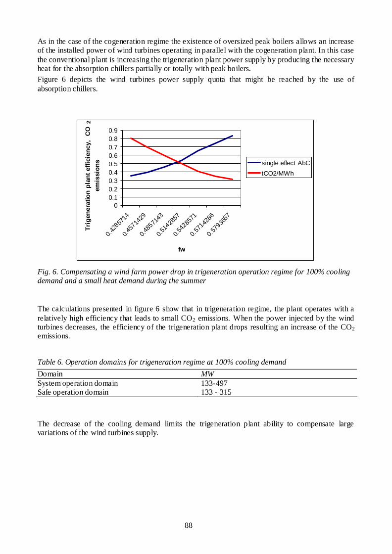
88

As in the case of the cogeneration regime the existence of oversized peak boilers allows an increase of the installed power of wind turbines operating in parallel with the cogeneration plant. In this case the conventional plant is increasing the trigeneration plant power supply by producing the necessary heat for the absorption chillers partially or totally with peak boilers. Figure 6 depicts the wind turbines power supply quota that might be reached by the use of absorption chillers.

00.10.20.30.40.50.60.70.80.9

0.428

5714

0.457

1429

0.485

7143

0.514

2857

0.542

8571

0.571

4286

0.579

3657

fw

Trig

ener

atio

n pl

ant e

ffici

ency

, CO

2 em

issi

ons single effect AbC

tCO2/MWh

Fig. 6. Compensating a wind farm power drop in trigeneration operation regime for 100% cooling demand and a small heat demand during the summer

The calculations presented in figure 6 show that in trigeneration regime, the plant operates with a relatively high efficiency that leads to small CO2 emissions. When the power injected by the wind turbines decreases, the efficiency of the trigeneration plant drops resulting an increase of the CO2 emissions.

Table 6. Operation domains for trigeneration regime at 100% cooling demand Domain MW System operation domain 133-497 Safe operation domain 133 - 315 The decrease of the cooling demand limits the trigeneration plant ability to compensate large variations of the wind turbines supply.

89

0

0.2

0.4

0.6

0.8

1

1.2

0.429 0.44 0.451 0.463 0.474 0.486 0.503

fw

Trig

ener

atio

n pl

ant e

ffici

ency

, CO

2 em

issi

ons

single effect ACtCO2/MWh

Fig. 7. Compensating a wind farm power drop in trigeneration operation regime for a 50 %

cooling demand

The safe operation domain for the 50% cooling demand is presented in table 7. The results are very close to the cogeneration operation during the winter period, trigeneration operation allowing in this case an increased electrical energy production for the wind farm during the summer.

Table 7. Operation domains for trigeneration regime at 50% cooling demand Domain MW System operation domain 157-473 Safe operation domain 157 - 315 5. Trigeneration operation regime with compressor chillers The use of compressor chillers for the construction of the trigeneration plant allows the increase of the wind turbine power quota.

0

0.2

0.4

0.6

0.8

1

1.2

0.47 0.49 0.51 0.54 0.56 0.58 0.61

fw

Trig

eera

tion

eff.,

CO

2 em

issi

ons,

co

ld d

eman

d Trigeneration plantefficiency Cold demand

tCO2/MWh

Fig. 8. Compensating a wind farm power drop in cogeneration trigeneration operation regime with compressor chillers

90

The use of compressor chillers lowers even further the minimum power of the trigeneration plant and that allows a further increase of the power injected by the wind turbines (figure 8). However there is also the downside of a direct link between the cooling demand of the consumers and the power that might be injected at one time by the wind turbines. Another downside is the necessity of both compressor and absorption chillers (when the power of the wind farm drops, the plant must use the absorption chillers operating with the heat produced by peak boilers). This also means that if the power of the wind turbines decreases (with the wind speed) the system has to buy some electrical energy from the grid ( 0SENE ). Even so the parallel operation with the trigeneration plant has some advantages because it decreases the electrical energy “imported” from the grid.

5. Conclusions The decentralisation of the electrical energy market tends to increase the pressure over the operating companies complicating the stability of the grids. Hydro power plants that might help the integration of the renewable sources, are in many cases operating with bilateral contracts with important (industrial) consumers, so the role of maintaining the grid stability is designated to conventional power plants (due to a higher price of the electrical energy). Parallel operation of wind turbines and conventional plants within a system is possible and reduces the negative effects over the energy system of one country. However a successful operation necessitates an understanding of the conventional plant operational limits. From the results presented in this paper it was possible to determine a safe system operation domain for each operation regime of the trigeneration plant. In other words cogeneration and trigeneration might increase the flexibility of the power supply of existing conventional plants and therefore these technologies could facilitate the integration of the renewable energy sources in the energy production mix. The success of the trigeneration plant in compensating the power variations of the wind turbines is directly related with the heat and /or cooling demand. The operation with absorption chillers ensures an increase of the safe power operation domain for the trigeneration-wind turbines system. This is possible if there is a shift of the heat delivered to the consumers or used by the absorption chillers from the combined heat and power plant to the peak boilers. The main advantage is in this case the increased power availability for the conventional plant. The compressor chillers allow an even further decrease of the power produced by the trigeneration plant so the installed power of the wind turbines might be even higher in this case. The problem with the compressor chillers is that the cooling demand dictates the power that might be produced by the wind turbines tacking into consideration the availability of the electrical energy from the national grid (ESEN). The paper shows also the necessity of a differentiated CO2 tax that takes into account that by partial load operation some conventional power plants allow an overall decrease of the CO2 emissions for the entire system, compensating the discontinuous operation of the wind turbines. A linear CO2 tax would only increase, in this case, an already high price of the energy.

Nomenclature Ew Electrical energy produced by the wind turbines Ecg Electrical energy produced by the CHP plant ECmpC Electrical energy consumed by the absorption chillers

91

Es Electrical energy produced by system Qcg Heat produced by the CHP plant Qpk Heat produced by the peak boilers QAbC Heat used by the absorption chillers Qs Heat produced by the system Cs Cooling demand COPAbC Coefficient of performance for the absorption chillers COPCmpC Coefficient of performance for the compressor chillers.

cg Total efficiency of the cogeneration plant [5]

References Journals : [1] Athanasovici V. and Dumitrescu I. S., - Global total efficiency of district heating systems,

Energetica Review, december 2005. Books and other monographs : [2] Liviu Ruieneanu General Method for the Analysis of Cogeneration Systems. LAP Lambert

Academic Publishing AG & Co KG., ISBN : 978-3-8443-2300-9, Germany, 2011 [3] Chic Wu, Thermodynamic cycles, Marcel Decker Inc., New York, 2003. [4] Meyer-Krahmer F, Kuntze U and Walz R, Innovation and Sustainable Development. Lessons

for Innovation Policies, Lessons for Innovation Policies. Physica, Heidelberg, 1998 [5] Flin D. Cogeneration – User’s Guide The Institution of Engineering and Technology, 2010 [6] Logan E, Roy R. Handbook of turbomachinery Marcel Decker Inc., New York, 2003. Conference Papers : [7] Ruieneanu, L., Mircea I., Technical-economical evaluation of CHP plants, WESC 2006,

Torino, Italy 2006 [8] Minciuc, E., Bitir-Istrate I. Patrascu R., Constantin C., Athanasovici V. Energetic analysis of

cogeneration, WEC Regional Energy Forum – FOREN 2004, Neptun, 13-17 June 2004 [9] V. Athanasovici, I. S. Dumitrescu A unitary method for the definition of technical indices

specific to medium and small scale cogeneration solutions, Energetica, Romania, April 1998. [10] Ruieneanu, L., Go ea, I. Considerations regarding the competitiveness of the CHP plants,

pg. 503-505, SIELMEN, Chisinau, Moldavia 2005. [11] Ruieneanu L., Mircea I , The unit costs method. A method for a CHP plant cots allocation

on both types of energy CNE 2004, Neptun Romania. 2004 [12] Monica Carvalho, Luis M. Serra*, Miguel A. Lozano Geographic evaluation of trigeneration

systems in the tertiary sector. Effect of climatic and electricity supply conditions. SDEWES 2009, Dubrovmik, Croatia.

Web references: [13] EUROPA- the official web site of the European Union. Official Journal of the European

Communities. Directive of the European parliament 2004/8/EC. [14] Greenhouse Gas Emissions from the U.S. Transportation Sector 1990-2003.EPA 420 R06 003

March 2006 www.epa.gov

PROCEEDINGS OF ECOS 2012 - THE 25TH INTERNATIONAL CONFERENCE ON EFFICIENCY, COST, OPTIMIZATION, S IMULATION AND ENVIRONMENTAL IMPACT OF ENERGY SYSTEMS


92

Advanced electromagnetic sensors for sustainable monitoring of industrial processes

Uroš Puca, Andreja Abinab, Anton Jegli c, Pavel Cevcd and Aleksander Zidanšeke a Jožef Stefan International Postgraduate School, Ljubljana, Slovenia, [email protected], (CA) b Jožef Stefan International Postgraduate School, Ljubljana, Slovenia, [email protected]

c Faculty of Electical Engineering, University of Ljubljana, Ljubljana, Slovenia, [email protected] d Jožef Stefan Institute, Ljubljana, Slovenia, [email protected]

e Jožef Stefan International Postgraduate School, Ljubljana, Slovenia, [email protected]

Abstract: Utilization of non-destructive and non-invasive methods for real-time monitoring of industrial processes is one of the challenging and desired tasks in industrial ecology. The aim of this work wa s to verify advanced electromagnetic (EM) sensors for material properties characterizing within industrial systems. To achieve this goal, we chose two EM sensors, an electromagnetic induction (EMI) sensor and ground penetrating radar (GPR). The operation of GPR is based on observation of EM waves reflections at the interface boundaries where the dielectric permittivity changes. We found out that the operation of the EMI sensor is in principle the same as that for GPR. In EMI method, the primary magnetic field produced by transmitter coil is changed in such a way that a higher density of magnetic flux lines occur due to the presence of metallic objects. Additionally, eddy currents occur which originate by metallic objects and have an important effect on the induction of the receiver coil field. In both methods, the changes due to material interactions with EM waves or magnetic fields are detected. The EMI method is used to characterize if the material within the industrial process i s metall ic or not. In case of non-metall ic material, the object is sent into the next level, where GPR is applied to determine the dielectric properties of the material. The proposed method is capable to monitor material flow through industrial system. In such a manner, an imperfect material or any other impurity could be detected and eliminated from the process. Furthermore, the eliminated material can be either reused in the same process or recycled in order to reduce disposal cost and energy consumption. Through modification and adaptation of GPR and EMI sensor, the applications of these technologies are expanding, and the advantages could also be used beneficially in the energy sector.

Keywords: Electromagnetic Induction Sensor, Ground Penetrating Radar, Industrial Ecology, Material Properties, Monitoring.

1. Introduction Nowadays, different techniques are used for non-destructive and non-invasive sensing. The utilization of such methods in industry provides the opportunity of real-time monitoring of industrial processes in a sustainable way [1-5]. Some sensing techniques are depicted in Fig. 1, which shows that the technology costs go up with the increased sensors availability and complexity. This paper is focused on two of those techniques - ground penetrating radar (GPR) and electromagnetic induction (EMI) sensor. Their applications have been growing rapidly and there was a great progress in the development of theory, technique and technology over the past few decades. The diversity of GPR and EMI applications includes a variety of areas [6-13], but in this work the focus will be on industrial applications such as concrete inspection in construction industry, subsurface infrastructure detection in transportation industry and water utility industry, food inspection and applications of these technologies in the energy sector. The aim of this work was to verify advanced electromagnetic (EM) sensors for material properties characterisation within feasible industrial systems. First, the basic principles of operation and physical background of GPR and EMI senor will be presented. Furthermore, the experimental setup will be explained to understand how these two sensors could be included into industrial processes. Experimental results will also be shown and discussed. We will demonstrate and evaluate how the

93

proposed methods are capable to monitor material flow through industrial system in such a manner that an imperfect material or any other impurity could be detected and eliminated from the process.

Fig. 1. Electromagnetic and similar sensing techniques used for monitoring and material properties characterizing.

2. Principles of EM sensors operation Electromagnetic waves comprise both electric and magnetic fields that oscillate at right angles to each other in the direction of propagation [14]. Furthermore, the EM waves are classified by frequency or by wavelength into radio wave, microwave, terahertz radiation, infrared wave, the visible region, ultraviolet, X-rays and gamma rays. Currently, various sensors exist in the range of all possible frequencies of EM spectrum [3-5]. The behaviour of EM waves as well as its interaction with matter depends on the selected working frequency. In this work the focus is on radio waves and microwaves which are used by GPR and EMI sensors. The operation of GPR is based on observation of EM waves’ reflections at the interface boundaries where the dielectric permittivity changes [15]. The operation of the EMI sensor is similar as that for GPR because both methods detect changes due to material interactions with EM waves or magnetic fields.

2.1. Physical foundation of GPR The GPR sensor uses electromagnetic wave energy to obtain information about the subsurface structures. Basically, this method operates by transmitting a very short EM pulse into the medium using an antenna at selected frequency. In practice, any GPR system contains a signal generator, a control unit, transmitting and receiving antenna. By using such a system configuration, the GPR measurements could be divided into two categories, reflection and transillumination, as shown in Fig. 2. The most useful is a reflection mode configuration in which a single transmitter and a single receiver are used. Typical GPR survey is conducted by moving a transmitter and receiver antenna, separated by a fixed distance, along a survey line [7]. For other more specialized applications multiple source and receiver configurations are recommended [16]. However, basic characteristics of the GPR investigation are related with a very high precision of the data, continuous surveying, highest survey resolution, entirely non-destructive and very fast collecting of data [17]. The principle of GPR is based on electromagnetic wave propagation. Maxwell’s equations are used to mathematically describe the physics of electromagnetic fields, while constitutive relationships provide a macroscopic description of how electrons, atoms, molecules, and ions respond to the application of EM field. These two sets of equations are used for describing the GPR signals. The propagation of the radar signals within the medium depends on the electromagnetic properties of the material, mainly the dielectric permittivity and electrical conductivity [18-19]. If there is a difference in dielectric permittivity between adjacent layers or objects in the medium the reflection

94

of incident EM radiation occurs. Synchronization between the transmitter and the receiver systems allows the determination of the time taken for the electromagnetic pulse to be reflected back. The travel time of the electromagnetic wave, which travels from the transmitter to the object in the medium and back to the receiver is known as two way travel time TWTT. The greater the contrast between media is the greater will be the amount of reflected energy. The proportion of reflected energy is given by the reflection coefficient R, which is determined by the contrast in radio wave velocities v or dielectric permittivities of adjacent media. The amplitude of reflection coefficient R is given by one of these two equations [7]:

)()(

21

21

vvvv

R (1)

12

12 )R (2)

However, the electromagnetic wave-matter interactions are usually expressed by the complex formulation of the dielectric permittivity:

rr jj ''''''~00 (3)

where 0 is the dielectric permittivity of a vacuum, ' and '' are the real and imaginary parts of the complex dielectric permittivity, and 'r and ''r are the real and imaginary parts of the relative complex dielectric permittivity. The real part carries the information about the electromagnetic energy, whereas the imaginary part is a measure of the energy loss in the material due to time varying field [20]. Radar signal velocity vm in low-loss medium like ambient air is related to the real part of a dielectric permittivity:

'cvm (4)

Although the velocity of radar waves can be expressed by:

TWTTdv m

2 (5)

where d is the distance between the GPR antenna and reflected point and TWTT is the two-way travel time of the GPR signal. The electrical response in medium is affected by various variables, such as selected frequency, material porosity, water content, aggregation state, component geometry, electrochemical interactions, temperature and density. Over the frequency range of 10 MHz – 1000 MHz, the real part of the dielectric constant does not appear strongly frequency dependent. When operating in this frequency range and if the medium is a good dielectric, the dependence of radar velocity on electrical conductivity is negligible. In such medium, the velocity of electromagnetic waves is related only to the real part of the dielectric constant [19].

Fig. 2. GPR measurements in reflection (a) and transillumination (b) geometry.

95

2.2. Physical foundation of EMI sensor Electromagnetic-induction is typically operated as an active sensor. EMI sensors are widely used to locate buried landmines [12-13, 21-23] by detecting the metal content in such objects. This sensor usually consists of a pair of concentric, circular coils, one of which is used to transmit electromagnetic waveform. The transmitted field induces a secondary current in any buried or hidden conducting object. A receiving coil senses the secondary field returned from the buried objects [21]. This is the foundation of the well known EMI method whereas the physics of EMI operation is completely described by Maxwell’s four equations [24]. Additionally, eddy currents occur which originate by metallic objects and have an important effect on the induction of the receiver coil field. These eddy currents are particularly expressed in case of conductor materials such as aluminium and not as much in case of ferro-magnetic materials such as iron. Unlike EMI sensors that can only detect mines with metal content, GPR is capable of detecting very low metal and plastic mines. In fact, the EMI principle is the basis of common metal detectors even those for treasure hunting on the beach, especially because they are not expensive and complex to produce. A partly or wholly metal object has a distinct combination of electrical conductivity, magnetic permeability, and geometrical shape and size. When this object is exposed to a low-frequency electromagnetic field, it produces a secondary magnetic field. When using EMI spectroscopy a distinct unique spectral signature could be obtained. This method could be used to identify different metal objects. EMI spectroscopy explores the frequency dependence of the EMI response in a broad frequency band in order to detect and characterize the object’s geometry and material composition [24].

Fig. 3. Principle of operation for EMI sensor.

3. Experimental setup Utilization of non-destructive and non-invasive methods for real-time monitoring of industrial processes is one of the challenging and desired tasks in industrial ecology. The realization of this task is possible with advanced EM sensors such as EMI sensor and GPR. In our experimental setup the EMI method is used within Level 1 to characterize if the material within the industrial process is metallic or not. Moreover, the proposed method is also capable to estimate the shape and orientation of detected metallic objects. In case of non-metallic material, the object is sent into the next level, where GPR is applied to determine the dielectric properties of the material by estimation of the reflection coefficient. Furthermore, the thickness of the sample could be estimated because the conveyor belt in this setup contains metal part which serves as a reference plate. However, the proposed method shown in Fig. 4 is capable to monitor material flow through industrial system. In such a manner an imperfect material or any other impurity could be detected and eliminated from the process.

96

Fig. 4. Method of real-time monitoring of industrial processes with EMI sensor and GPR.

3.1. Monitoring by GPR The research work was conducted using a commercial georadar system manufactured by Mala Geoscience Inc. The GPR system was equipped with a 1.6 GHz antenna. The software for data acquisition run in the GPR processing unit, from where the raw data were transferred to the computer used for further calculations. The proposed method for reflection coefficient calculation is based on analyzing the raw GPR signals. Each 1-D GPR target response provides some unique information; therefore the signal needs to be acquired in an appropriate way. As a reference signal we used the reflection from the large metal plate which was placed behind the plastic sample holder as shown in Fig. 5. The sample holder filled with dry sand was located on the same place in each measurement with the constant distance from the antenna which was in the range of few centimetres. The reflected sample signal contains both reflections from the top and the bottom of the sample, thus the reflection coefficient of the material inside the sample holder could be estimated. This is the reason why we extracted the early-time response from the GPR signal and excluded the late-time response, which is always distorted by other uncontrollable environmental factors. Later on, the reference signal through the ambient air is subtracted from the measured signal of the dry sand. The subtraction between reference signal and sample signal at two different distances between antenna and metal plate is shown in Fig. 9.

97

Fig. 5. The measurement setup for GPR data acquisition with a reference metal plate and sample holder.

3.2. Monitoring by EMI The scenario for EMI monitoring comprised EMI sensor composed of four probes mounted on a wooden pole (Fig. 6). Moreover, the home-made EMI sensor was moving on a quadratic holder made from wood to reduce destructive interferences from other objects. For the investigation purposes, samples with simple circular and rectangular cross sections were selected. For carrying out laboratory experiments we consider dynamic sensor system and static samples which were located on the wooden plate with the constant distance from the sensor which was in the range of few centimetres. The investigated area was limited with dimensions of 45 cm by 85 cm. However, the inverse case is also possible where EMI probes are fixed on a pole, e.g. above the production line and as such serve as an in-line monitoring tool. In such a manner, EMI can be applied in real-time monitoring of material flow through industrial systems. Special software was prepared to acquire signals from all four probes simultaneously. The raw signals in a matrix form were imported in Matlab programming environment. In order to obtain a more realistic circular or rectangular cross section of the detected objects the 2-D interpolation between the matrix elements was applied. Furthermore, the obtained plots were smoothed using MatLab’s built-in cubic interpolation function. The final results were visualized as an intensity plot.

Fig. 6. The measurement setup for data acquisition with the EMI sensor composed of four individual probes.

98

4. Results and discussion The proposed method for reflection coefficient calculation is based on analyzing the raw GPR signals. As a reference signal we used the reflection from the large metal plate which was placed behind the sample holder. The sample located in front of the metal plate modifies the signal shape and its amplitude. Hence, from the signals fingerprint one can notice that the sign of the polarization is changed where the sample is present. In Fig. 7 the sign of the polarization is changed at 51st sample whereas in Fig. 8 this change is shifted for 7 samples to the right corresponding to the longer distance between the GPR antenna and reference plate. For accurate reflection coefficient calculation some initial optimization parameters had to be determined, such as sampling rate and time window in ns. Size of the time window was set to 10.781626 ns. The total number of samples was 176. These two parameters are used for signal velocity calculation. With the subtraction function between the reference signal and sample signal it is possible to determine the top and the bottom of the sample. In Fig. 9 the bottom of the sample can be clearly identified as a maximum positive peak whereas the end of the ground signal is defined as a point where the difference between the signals starts to rise. The distance between these two points is actually the distance between a GPR antenna and reference plate. For instance, at distance of 12 cm this difference counts 19 samples, at distance of 18 cm it counts 26 samples. Within this distance both media ambient air and dry sand are included. Thus, it is important to recognize the point representing the top of the sample which is in our case the second positive peak at 41st and 48th samples. By knowing all these locations in plot and distance from antenna to metal plate, one can calculate the signal velocity through the air and the sample by equation:

'2 c

TWTTdvm (6)

Fig. 7. The comparison between acquired signals with and without a sample of dry sand at a distance of 12 cm between antenna and reference plate.

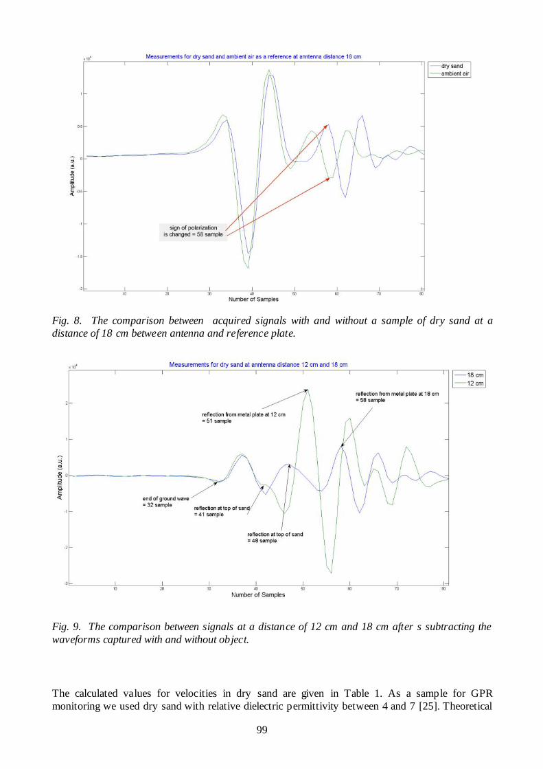
99

Fig. 8. The comparison between acquired signals with and without a sample of dry sand at a distance of 18 cm between antenna and reference plate.

Fig. 9. The comparison between signals at a distance of 12 cm and 18 cm after s subtracting the waveforms captured with and without object.

The calculated values for velocities in dry sand are given in Table 1. As a sample for GPR monitoring we used dry sand with relative dielectric permittivity between 4 and 7 [25]. Theoretical

100

value of the reflection coefficient R given by equation (2) and is in the range between 0.333 and 0.451. Practically estimated reflection coefficient R given by equation (1) has a value of 0.428 for a distance of 12 cm and 18 cm between antenna and reference plate. The estimated and calculated values of reflection coefficients are given in Table 1. Additionally, range detection could be also performed by GPR technique. Thus, the distance from a GPR antenna to the object could be estimated. If the distance from the antenna to the reference plate is constant, one can determine the thickness of the sample as well. This concept could be adapted to in-line and real-time monitoring of material samples within various industrial processes which is a key for ensuring final quality of products as well as eliminating waste from the industrial process. If the production lines contain an embedded metallic layer it serves as a reference, similar to the metal plate used in our experiment. The wider area where material samples are placed can be sensed by an array of GPR antennas. Hence, the reflection coefficient calculated with the above described method can be acquired from various sites of the sample simultaneously. In case of any impurity or imperfection within the homogenous material, the value of reflection coefficient at this site will differentiate from the rest of the sample. For instance, this technology could be used for in-line monitoring of cracks and voids inside concrete slabs as well as for detection of impurities within the food samples (e.g. flour) or any other solid samples with a significant difference in the reflection coefficient between the impurity and the surrounding homogenous material.

Table 1. Signal velocities for ambient air and dry sand calculated from acquired signals

Medium Distance (cm)

Signal velocity (cm/ns)

Estimated reflection coefficient

Calculated reflection coefficient ( = 4-7)

12 13.059 0.428 0.333-0.451 dry sand 18 13.059 0.428 0.333-0.451

The EMI method is used to characterize if the material within the industrial process is metallic or not. Apart from this, we also found out that different metallic objects give various EMI responses. Fig. 10 shows four different EMI responses from four probes acquired synchronously. The probes are equidistantly positioned on a wooden pole. In this case, we investigated two rectangular objects with different dimensions. Probe 1 and probe 2 were located on the outside of the pole, therefore only the larger object was detected with all four probes. The smaller object was visible only for probe 2 and probe 3.

Fig.10. Four different EMI responses from four probes of EMI sensor acquired synchronously.

The raw EMI responses were recorded in a matrix form. With basic imaging method based on cubic interpolation 2-D images were obtained. From these images one can notice that not only the shape

101

(Fig. 12a) and orientation (Fig. 11) of the objects could be detected but also some information regarding metal material characterization could be defined. In Fig. 12b there is a major difference in EMI responses between aluminium and iron objects due to the eddy currents which originate by metallic objects and they are particularly expressed in case of conductor materials such as aluminium and not as much in case of ferromagnetic materials such as iron.

Fig.11. 2-D EMI images of different objects orientation, parallel (a) and inclined (b.

Fig.12. 2-D EMI images of different object shapes (a) and various material composition (b)

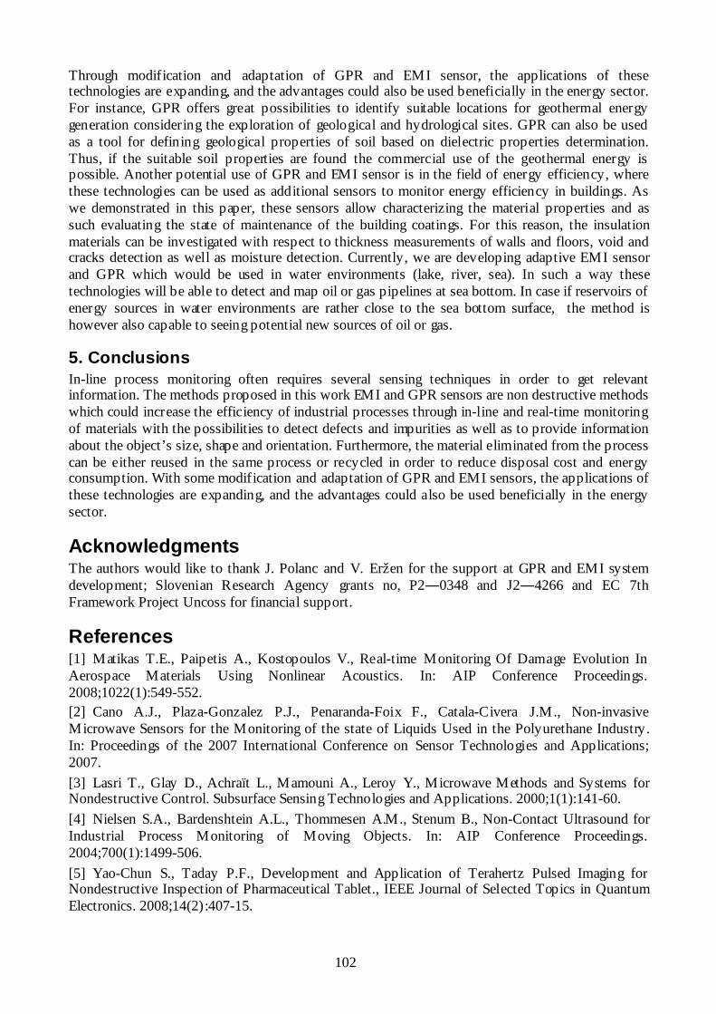
102

Through modification and adaptation of GPR and EMI sensor, the applications of these technologies are expanding, and the advantages could also be used beneficially in the energy sector. For instance, GPR offers great possibilities to identify suitable locations for geothermal energy generation considering the exploration of geological and hydrological sites. GPR can also be used as a tool for defining geological properties of soil based on dielectric properties determination. Thus, if the suitable soil properties are found the commercial use of the geothermal energy is possible. Another potential use of GPR and EMI sensor is in the field of energy efficiency, where these technologies can be used as additional sensors to monitor energy efficiency in buildings. As we demonstrated in this paper, these sensors allow characterizing the material properties and as such evaluating the state of maintenance of the building coatings. For this reason, the insulation materials can be investigated with respect to thickness measurements of walls and floors, void and cracks detection as well as moisture detection. Currently, we are developing adaptive EMI sensor and GPR which would be used in water environments (lake, river, sea). In such a way these technologies will be able to detect and map oil or gas pipelines at sea bottom. In case if reservoirs of energy sources in water environments are rather close to the sea bottom surface, the method is however also capable to seeing potential new sources of oil or gas.

5. Conclusions In-line process monitoring often requires several sensing techniques in order to get relevant information. The methods proposed in this work EMI and GPR sensors are non destructive methods which could increase the efficiency of industrial processes through in-line and real-time monitoring of materials with the possibilities to detect defects and impurities as well as to provide information about the object’s size, shape and orientation. Furthermore, the material eliminated from the process can be either reused in the same process or recycled in order to reduce disposal cost and energy consumption. With some modification and adaptation of GPR and EMI sensors, the applications of these technologies are expanding, and the advantages could also be used beneficially in the energy sector.

Acknowledgments The authors would like to thank J. Polanc and V. Eržen for the support at GPR and EMI system development; Slovenian Research Agency grants no, P2 0348 and J2 4266 and EC 7th Framework Project Uncoss for financial support.

References [1] Matikas T.E., Paipetis A., Kostopoulos V., Real-time Monitoring Of Damage Evolution In Aerospace Materials Using Nonlinear Acoustics. In: AIP Conference Proceedings. 2008;1022(1):549-552. [2] Cano A.J., Plaza-Gonzalez P.J., Penaranda-Foix F., Catala-Civera J.M., Non-invasive Microwave Sensors for the Monitoring of the state of Liquids Used in the Polyurethane Industry. In: Proceedings of the 2007 International Conference on Sensor Technologies and Applications; 2007. [3] Lasri T., Glay D., Achraït L., Mamouni A., Leroy Y., Microwave Methods and Systems for Nondestructive Control. Subsurface Sensing Technologies and Applications. 2000;1(1):141-60. [4] Nielsen S.A., Bardenshtein A.L., Thommesen A.M., Stenum B., Non-Contact Ultrasound for Industrial Process Monitoring of Moving Objects. In: AIP Conference Proceedings. 2004;700(1):1499-506. [5] Yao-Chun S., Taday P.F., Development and Application of Terahertz Pulsed Imaging for Nondestructive Inspection of Pharmaceutical Tablet., IEEE Journal of Selected Topics in Quantum Electronics. 2008;14(2):407-15.

103

[6] Chen C., Zhang J., A Review on GPR Applications in Moisture Content Determination and Pavement Condition Assessment. In: Proceedings of ACE, 2009. [7] Knight R., Ground penetrating radar for environmental applications. Annu Rev Earth Planet Sci. 2001;29:229-55. [8] Hubbard S., Jinsong C., Williams K., Rubin Y., Peterson J., Environmental and agricultural applications of GPR. Advanced Ground Penetrating Radar. In: Proceedings of the 3rd International Workshop on IWAGPR; 2005 May 2-3, 2005. [9] Olhoeft G.R., Applications and frustrations in using ground penetrating radar. Aerospace and Electronic Systems Magazine, IEEE. 2002;17(2):12-20. [10] Olhoeft G.R., Applications and limitations of ground penetrating radar. SEG Technical Program Expanded Abstracts. 1984;3(1):147-8. [11] Lai W.L., Kind T., Wiggenhauser H., Using ground penetrating radar and time-frequency analysis to characterize construction materials. NDT & E International. 2011;44(1):111-20. [12] Druyts P., Craeye C., Acheroy M., Volume of Influence for Magnetic Soils and Electromagnetic Induction Sensors. IEEE Transactions on Geoscience and Remote Sensing. 2010;48(10):3686-97. [13] Sezgin M., Kaplan G., Birim M., Bahadirlar Y., Buried metalic object identification by EMI sensor. 2007: SPIE. [14] Manoj G., Eugene W.W.L., Introduction to Microwaves. Microwaves and Metals. Singapore: John Wiley & Sons; 2007. [15] Ghasemi F.S.A., Abrishamian M.S., A novel method for FDTD numerical GPR imaging of arbitrary shapes based on Fourier transform. NDT & E International. 2007;40(2):140-6. [16] Jol H.M., Ground penetrating radar: Theory and applications. First ed: Elsevier Science; 2009. [17] Cukavac M., Klemcic G., Lazovic C., Reconstruction Of Buried Objects by Implementation of Ground-penetrating radar technique: Example on Roman Tomb in Brestovik (Serbia). In: Proceedings of the International Conference on Geoarchaeology & Archaeomineralogy; 2008: 333-338. [18] Annan A.P., Electromagnetic Principles of Ground Penetrating Radar. In: Jol H.M., editor. Ground Penetrating Radar Theory and Applications. 1st ed. Oxford: Elsevier; 2009. p. 3-40. [19] Gloaguen E., Chouteau M., Marcotte D., Chapuis R., Estimation of hydraulic conductivity of an unconfined aquifer using cokriging of GPR and hydrostratigraphic data. Journal of Applied Geophysics. 2001;47(2):135-52. [20] Stuerga D., Microwave–Material Interactions and Dielectric Properties, Key Ingredients for Mastery of Chemical Microwave Processes. In: Loupy A, editor. Microwaves in Organic Synthesis. 2nd ed.; 2006. p. 1-61. [21] Collins L., Gao P., Makowsky L., Moulton J., Reidy D., Weaver D., Improving detection of low-metallic content landmines using EMI data. In: Proceedings of the Geoscience and Remote Sensing Symposium, 2000. [22] Ho K.C., Collins L.M., Huettel L.G., Gader P.D., Discrimination mode processing for EMI and GPR sensors for hand-held land mine detection. IEEE Transactions on Geoscience and Remote Sensing. 2004;42(1):249-63. [23] Xuejun L., Carin L., Application of the theory of optimal experiments to adaptive electromagnetic-induction sensing of buried targets. IEEE Transactions on Pattern Analysis and Machine Intelligence. 2004;26(8):961-72. [24] Won I.J., Keiswetter D.A., Bell T.H., Electromagnetic induction spectroscopy for clearing landmines. IEEE Transactions on Geoscience and Remote Sensing. 2001;39(4):703-9. [25] Rudge A.W., The Handbook of antenna design. London: Peter Peregrinus Ltd.; 1983.



104

Assessment of stresses and residual life of plant components in view of life-time extension of

power plants

Anna Stoppatoa(CA), Alberto Benatob and Alberto Mirandolac a D.I.I. University of Padova, Padova, Italy, [email protected] b D.I.I. University of Padova, Padova, Italy, [email protected]

c D.I.I. University of Padova, Padova, Italy, [email protected]

Abstract: The deregulated energy market requires strong, irregular and discontinuous operation in order to meet the user demand and produce energy mainly during peak hours, when the electricity price is higher. The increasing number of plants powered by non-predictable renewable sources and of cogenerative units has amplified this need. For this reason, over the last decade new more flexible strategies in thermal power plants and systems management have been applied, which ensure greater income in the short term, but likely cause a lifetime reduction of the most critical components, due to thermo-mechanical fatigue, creep and corrosion. A procedure aimed at evaluating this extra cost related to a flexible operation, and at assisting the management decision about power plants’ operation and maintenance scheduling has been implemented by the Authors. The procedure, on the basis of the historical data, predicts the residual life of the most critical components, considering the effects of creep, thermo-mechanical fatigue, welds, corrosion and oxidation, as a function of the past and the forecasted operation strategy. The core of this procedure is the simulation tool, able to evaluate the variation of the most important thermodynamic parameters versus load during the transitory periods and then to estimate the creep and fatigue stresses on plant devices. In this paper the model for the analysis of a combined power plant will be presented. It permits to simulate the load variation of the plant also during start-up and shut-down. The velocity of these variations is taken into consideration too. Then, the stresses of the most critical components are calculated and the related damage evaluated. Finally, the residual lifetime can be estimated and the consequences on the long term profit of the plant assessed.

Keywords: Deregulated market, Combined plants, Super-heater, Creep-fatigue model, Sustainability.

1. Introduction The gradual liberalization of the gas and electricity markets in Europe [1-2] has caused growing competition among different electricity producers and this makes more and more important optimizing management strategies and plant control in order to reduce production costs. This optimization must also take into account the severe environmental laws which restrict the operating margins of power plants [3]. The operating economy is therefore essential for all the electric operators since it is the requisite for the survival in the energy market, but the variability of fuel costs [4], the new and more efficient technology systems [5], the connection to the grid of many plants powered by renewable sources, often small in size and not able to plan their production [6-7], the daily variability of electricity demand and price [8] pose complex problems to the plant operator which has to develop operational models aimed at improving the system management in terms of efficiency, flexibility and reliability.

105

All these aspects result in new strategies for plant and systems management: strongly irregular and discontinuous operation of power plants is required in order to meet the user demand, satisfy the CO2 emission limits and maximize profits by producing as much as possible during peak hours, when the electricity price is higher, while stopping the plant or greatly reducing the load during off-peak hours. Consequently, many plants have to work in the so-called “two shift run” [9-11], operating for 12-15 hours/day, and usually stopping for the whole weekend. Essential characteristics for the correct functioning of the power system is the ability to satisfy the load changes required by the electricity demand (especially the demand for short term, that has a higher profit) and operating at minimum load during off-peak periods. Therefore, each unit should have design features that make it capable to work either at high loads or at a technical minimum and make night and weekend shutdowns with short time restart. Gas turbines and combined plants, that are powered by expensive high-quality fuel, which are more flexible than other thermal power plants, are especially asked to make frequent and rapid load variations, but also steam power plants are often operated at variable load with several stops [10,12]. Going from a basic to a flexible usage involves the need of verifying the suitability of plants to develop a different role for which they were designed and studying types of plant management to reduce problems related to flexibility. This type operation guarantees greater profits in the short term, but can cause a reduction in the lifetime of the most critical components, due to thermo-mechanical fatigue loadings. Since the correct target of good management is to obtain the best average performance during the whole life of the system, the decision makers need suitable tools that are able to give information about the long-term consequences of the operation choices. The boilers, in particular the parts at higher temperature, gas and steam turbines are subjected to higher thermo-mechanical cycles due to an increase of heating velocity and to the number of these transitional periods. Each cycle damages the components and the accumulated damages end up causing frequent breakdowns and unplanned maintenance. Moreover, the methods used to start and stop the plant influence its reliability and its life expectancy. The Authors in the past have investigated [13] the relationship between a plant’s operation and its components’ residual life. A model to assess damage from creep and thermo-mechanical fatigue has been proposed and its application was presented to find the cumulative mechanical damage of the most critical components of thermoelectric power plants. The effects of corrosion and erosion on the residual life are considered too and included in the model of damage. The presence of weak points in the devices, such as welding in the pipes of boilers, where the problems are accentuated, is considered too. This model has been introduced into a procedure for power plant on-line monitoring, control, production and maintenance scheduling already presented [14-15]. It can be used to evaluate the effect of the current management strategy in terms of reduction of residual life. To take into account the high uncertainty of the electricity market, the procedure has been improved with the possibility of modifying the production strategy during operation. In this paper, the focus is on the combined gas-steam power plants which currently gives the 57.5% of the electric energy produced in Italy (69.4% of that from thermal plants) and for this reason, are now the most interesting in regard to operating flexibility problems. Moreover, the spinning and cold reserve service is a prerogative of these plants. This will permit greater profits, but asks for: Reducing characteristic time of start-up and transitional load. Extending the field of possible operating conditions by increasing the peak power or reducing

the technical minimum load. Higher recurrence of transient conditions already provided.

106

2. Combined cycle Gas cycles are flexible while steam ones are “slow”, so during transitional operation of a combined plant the Heat Recovery Steam Generator (HRSG), where the coupling of two cycles actually occurs, must work as a thermal flywheel and for this reason it is subjected to high thermo-mechanical fatigue. ASME (section-Power Boiler Code) [16], British Standard (BS1113) [17], EN 12952[18] and TRD301 [19] are guidelines for HRSG design taking into account these problems. The most stressed element is the high temperature super-heater (SH), which is subject to high temperatures and pressures; so during transitional operation the thermo-mechanical fatigue is added to creep phenomenon. Some typical examples of how cycling creates or enhances damaging the mechanism are given below: Creep damage by definition is caused by a prolonged exposure to high temperature and stress.

Creep may be the only process which is not caused or enhanced by cycling. However if the creep is coupled with fatigue due to cycling, the damage will be much higher than that occurring if the same fatigue or creep is working alone.

Fatigue damage is the most prevalent action affecting the boiler life and is a direct consequence of cycling. For example, for rapid starting, the SH is exposed to high temperature on the outside of tubes and headers whereas inside may still be cool, while at shut down cool gasses are sent on hot surfaces. Similarly, the condensed steam in the tubes after shut down impinges on hot surfaces if condensate remains in the tubes. The high pressure components are more vulnerable to top fatigue effects due to higher thickness.

Thermal shock: condensate in the super-heater would result in thermal shock to the inner surface of the tubes hand headers.

Oxidation: is caused by the exposure of the metal to high temperature in comparison to design specifications. Oxidation and corrosion can happen inside and outside due to gas or steam. The reaction with water results in corrosion this is due to cycling or because of water treatment failure.

Differential expansion: uneven heating of tubes due to flow and temperature bad distribution causes adjacent tubes to expand differently. This problem can also present itself when devices made of difference materials or having different thickness are connected; for example between headers and tubes.

Operation in a two-shift regime has two main effects on steam turbines: Thermal fatigue and creep/thermal fatigue associated with thick walled component, including

start and stop valves and HP and IP turbines inlet belts. Mechanical fatigue as a result of load and speed variations. It arises from two sources: a) during

the run up, the passages of critical speed where vibration levels increase; b) the very high centrifugal stress on the route area of blades, which is more important in LP stages. Other problems are related to the overheating of turbines as a result of windage, to differential expansion of rotors and casings, to erosion as a result of oxide impact of blades.

2.1. The model Mechanical parameters in the devices, that are stress and strain deriving from creep and thermo-mechanical fatigue, are used to calculate the cumulative mechanical damage to each single component. They depend on the thermodynamic variable trends which define the energy conversion process, both during constant and transient operation. A model of a simple one level combine cycle has been built by means Dymola software [20] and CombiPlant Library [21] in order to estimate the thermodynamic variable trends during different operation modes. Since at the present the main focus is on the HRSG the gas cycle has been modeled as a hot gas source.

107

The design power of the plant is 40 MW of which 13 MW from steam section. The load variation is simulated using a control on the gas sub-section. The layout of the model is reported in Fig. 1. It also includes all the control systems, whose role is very important during load variations. Drum vent, admission valves and pump speed control are implemented. They are in charge of maintaining the correct water level in the drum. Steam temperature control is needed to avoid that the steam temperature from the HRSG is too high. The geometry of all the devices (number, length and diameter of pipes in the heat exchangers and their configuration, turbine and pump dimensions, connection pipes dimensions), their materials and turbine and pump maps have been introduced into the parameters windows of Dymola Software.

Fig. 1. Model of the Combined Plant.

2.2. Model results The response of the steam section is analyzed using the Model reported in Fig. 1. To evaluate the influence of the load variation velocity on devices lifetime, Authors studied load variations from design point to the technical minimum (40% of design electric power). The simulations differ for the duration of rise and fall times on the gas side (from 20 to 40 minutes) and for the duration of the operation at minimum load between two successive transient periods (from 15 to 120 minutes). Fig. 2 shows the gas and steam mass flow rate and the mechanical power by the steam turbine for a transient period of 20 min. As we can see, steam plant time constant is about twice than that of gas while the two trends are very similar. In Fig. 3 the water level in the drum is shown during the fastest load variation. It is evident that both raise and fall do not present control problems.

108

Fig. 2. Trend of gas and steam mass flow rate and of steam turbine mechanical power (W) vs. time (s) for a load variation from design to minimum load in about 20 min.

Fig. 3. Water level in the drum (m) and drum air vent signal vs. time (s).

During transient operation, plant components are subject to variations of pressure and temperature that cause thermal stress and thermo-mechanical fatigue. The super-heater is one of the most critical components. For this component, Fig. 4 shows the medium diameter wall temperature trends vs. time in different positions along the flow path for the most severe (i.e. rapid) raise and fall conditions. As we can see, there is a large temperature variation along the longitudinal development of each tube (more than 120°C from the wall near gas inlet and that near gas outlet at design point). This difference is about 70°C lower at minimum load, while reaches higher values during raise time. Note also that the maximum wall temperature is about 20°C higher during transitory that its design value; at minimum load this temperature is about 220°C lower.

109

Fig. 4. Medium diameter wall temperature (°C) trends in super heater vs. time in different positions along the longitudinal development form gas inlet [4] to gas outlet [1].

Fig. 5. Gas, steam and wall inner and outer diameter temperature (°C) trends in the hottest point of the superheater (i.e. at gas inlet).

In addition, due to the heat transfer from hot gas to colder steam, there is a temperature difference between inner and outer diameters of pipe walls. Fig. 5 shows the temperature trends for the hottest point: there are about 4.3°C along the pipe thickness (2.5 mm) at design point, but this value vary with load up to about 0°C at minimum load. This variation causes a thermo-mechanical fatigue stress, too. For the same load variation, the steam pressure varies from 64.1 bar to about 15.1 bar.

2.2. Life time reduction calculation

110

The super heater is made of AISI SA335P91 (P91) with a high mechanical strength up to 650 – 700°C. This material is commonly used for the super-heaters of high performance three level combined cycles, but it could be used also for simpler plants. Pipes have an inner radius of 10 mm and a thickness of 2.5 mm. As said, all the pressure and temperature variations during transient period generate thermo-mechanical fatigue stress in addition to creep. Using the model described in [15], the strain range in the most sollecited point of super-heater wall, which is the inner diameter in the hottest position, has been evaluated during each cycle as a function of steam pressure and temperature variations. Then, by means of the experimental Manson-Coffin curve of P91, reported in Fig.6 [16], the cycles number to complete failure has been calculated for each simulation.

Fig. 6. Manson-Coffin curve for P91 at 540°C [16].

For the load variation from the design point to the technical minimum in 20 minutes analysed in the previous section, the strain range is 0.003566. It corresponds to about 1400 cycles before failure. For a load variation with double time constants (about 40 min from design to minimum load) the strain range is 0.003566 and the life is about 1750 cycles. This difference is mainly related to the lowest temperature peak in the most stressed point, as shown in Fig.7. In both these cases, the duration of operation at the minimum load before the following raise up has been simulated 120 min long, while the operation at design load is 60 minutes long. If this duration is reduced up to 30 minutes, the effects on life time is not significant, but if it is reduced to 15 minutes the strain range becomes 0.0035736 corresponding to 1200 cycles before rupture, always with a transient duration of 20 minutes. This reduction is due to an increase in the peak temperature, caused by the not complete achievement of stationary conditions on steam side between load fall and raise. Considering a management strategy aimed at the maximum production only when electricity prices are higher, where the plant operates at design load from 9 am to 6 pm, and at the minimum technical from 6 pm to 9 am, these results correspond to a life time of about 4 years if the hypothesis of load variation within 20 minutes, of 5 years if the variation is within 40 minutes.

0,001

0,01

0,1

1

1,00E+01 1,00E+02 1,00E+03 1,00E+04 1,00E+05 1,00E+06 1,00E+07 1,00E+08 Nd

T = 540 °C

111

Fig. 7. Wall external diameter temperature (°C) trends in the hottest point of the superheater for two different velocities of load variations.

3. Steam plant turbine A model was also built of a steam turbine for thermal power plant having seven extractions. The turbines are very critical in steam plants, since they often have been not designed for a cyclic operation and so have small axial and radial clearances between rotors and casings and thick walls, while the bypass of the turbine during start-up is not present. The model was tested using data derived from tests at stationary load from an existing plant sized 320 MW. Subsequently, authors used this model to implement the transition from nominal power to zero power; situation that normaly occurs during an operation to stop the plant or the occurence of a break. Fig. 6 shows the scheme of the turbine model. In Fig. 7 the measured power generated by the HP section during a shut down for a out of load problem is presented. Fig. 8 reports the simulated mass flow rate and turbine inlet pressure trends for the same event. There is a good correspondence between measured during a transient period and simulated values for temperature and pressure of drains. Also in this case, these results can be used to evaluate the stress and strain on turbine blades and casing and consequently the lifetime reduction due to a sudden shut down.

Fig. 8. Scheme of a 320 MW turbine model.

112

Fig. 9. Trend of power (MW) generated by the HP turbine section vs. time (s).

Fig. 10. Trend of mass flow rate (kg/s) and inlet pressure (bar) for the HP turbine vs. time (s).

4. Conclusions Some models for the simulation of plants operation during load variations have been presented. They can be used to calculated thermodynamic variable trends which influence creep and thermo-mechanical fatigue damage in plant devices. So, the lifetime of devices can be forecasted as a function of operation management. The models permit to simulate management strategies different: for number of annual hot or cold start-ups, velocity of load variations, for hours of operation at design and off-design load. The results give a comparison among strategies in terms of devices lifetime, which can be translated in economic terms.

References [1] Directive 2003/54/EC of the European Parliament and of the Council of 26 June 2003

concerning common rules for the internal market in electricity and repealing Directive 96/92/EC

[2] Directive 2009/72/EC of the European Parliament and of the Council of 13 July 2009 concerning common rules for the internal market in electricity and repealing Directive 2003/54/EC]

[3] Italian National Emission Plan, D.lgs. April 4, 2006, n. 216 and its modifications (in Italian). [4] DOE/EIA International Energy Outlook 2011- Available at: <www.eia.gov> [accessed

2.2.2012].

113

[5] Roques F.A., Technology choices for new entrants in liberalized markets: The value of operating flexibility and contractual arrangements. Utilities Policy 2008; 16(4): 245-253.

[6] Tsao C.C., Campbell J.E., Chen Y., When renewable portfolio standards meet cap-and-trade regulations in the electricity sector: Market interactions, profits implications, and policy redundancy. Energy Policy 2011; 39 (7): 3966-3974.

[7] Milstein I., Tishler A., Intermittently renewable energy, optimal capacity mix and prices in a deregulated electricity market. Energy Policy 2011; 39 (7): 3922-3927.

[8] GME Statistics Monitoring-Electricity Market- summary data - Available at: http://www.mercatoelettrico.org/en/Statistiche/ME/DatiSintesi.aspx [accessed 2.2.2012].

[9] Concari S, Fedeli G., Cyclic Operation Experience at ENEL with Conventional Thermal Power Plant, Proceedings of the International seminar “Cyclic Operation of Power Plant- Technical, Operation and Cost Issues. London, 25-27 June 2001.

[10] Dukashe MP, Nieuwoudt T, Begg J., Operational Experience of two shifting Large Coal Fired Unit, Proceedings of the International seminar Cyclic Operation of Power Plant-Technical, Operation and Cost Issues, London, 25-27 June 2001.

[11] Chow J, Ho K, Du X, Lee HS, Pearson M. Experience from extensive two-shift operation of 680 MW coal/gas fired Units at Castle Peak, Hong Kong, Proceedings of the International seminar Cyclic Operation of Power Plant- Technical, Operation and Cost Issues, London, 25-27 June 2001.

[12] Lefton SA, Besuner P, Grimsrud P, Kunts T. Experience in Cycling Cost Analysis of Thermal Power Plants in North America and Europe, Proceedings of the International seminar Cyclic Operation of Power Plant- Technical, Operation and Cost Issues, London, 25-27 June 2001

[13] Carraretto C, Lo Casto E, Meneghetti G, Polo F, Stoppato A., Comparison Among Thermo-Mechanical Fatigue Criteria in The Context of Long-Term Power Plants Optimisation, Proceedings of ECOS 2007, Padova – Italy, June 25-28 2007: 1637-44.

[14] Mirandola A, Lo Casto E, Stoppato A., A procedure for the evaluation of residual life of steam Power plant devices. Proc. of the 22nd International Conference on Efficiency, Cost, Optimisation, Simulation and Environmental Impact of Energy Systems ECOS 2009, Iguaçu (Brazil).

[15] Lo Casto E, Mirandola A, Stoppato A., Evaluation of the effects of the operation strategy of a steam power plant on the residual life of its devices. Energy, The International Journal, 2010; 35: 1024-32

[16] ASME Code. Boiler and pressure vessel code. Section II, III, New York, USA, 2001. [17] British Energy. R5, Assessment procedure for the high temperature response of structures. Issue 3,

Gloucester, UK, 2003. [18] UNI EN 12952-5:2011 Water-tube boilers standards [19] TRD 301 Annex1 – Calculation for cyclic loading due to pulsating internal pressure or

combined changes of internal pressure and temperature [20] Elmqvist H, Brück D, Otter M. Dymola User’s Manual, Dynasim AB, Research Park Ideon,

Lund, Sweden, 1996. [21] CombiPlant Library, Modelon AB in:ww.modelica.org/libraries/CombiPlant.



114

Control Strategy for minimizing the electric power consumption of Hybrid Ground Source

Heat Pump System

Zoi Sagiaa, Constantinos Rakopoulosb

National Technical University of Athens, School of Mechanical Engineering, Department of Thermal Engineering,

Laboratory of Thermal Processes, 9 Heroon Polytechniou St., Zografou Campus, 15780 Athens, Greece [email protected], CA [email protected]

Abstract: Hybrid Ground Source Heat Pump Systems (HGSHPSs) which include cooling towers are widely used so as to improve Ground Source Heat Pump Systems (GSHPSs) efficiency in cooling dominated applications. A Greek office building with total cooled area 1000 m2 is examined. The whole system is modelled using TRNSYS 17. System’s operation is optimized using TRNOPT 17 so as to meet the maximum cooling load during the net cooling period, when no heating loads occur, by minimizing Ground Heat Exchangers (GHEs) depth. Three control strategies, based on continuous observation of critical temperatures, are applied to the optimized system. Each strategy attempts to achieve a further optimization of HGSHPS’s operation by minimizing the electric power consumption. In the first one, the cooling tower is turned on when the difference between the fluid temperature exiting heat pumps and ambient air wet bulb temperature exceeds 10 oC. In the second one, the cooling tower is on when the fluid temperature exiting GHEs is greater than 28 oC. In the third one, the cooling tower starts to operate when the fluid temperature exiting heat pumps is greater than 32 oC. Each of these control points is normalized by the fluid temperature exiting the hot side of Heat Exchanger which comes in between the ground loop and the Closed Circuit Cooling Tower loop. The new set points define three new control strategies which are examined so as to achieve a further improvement to HGSHPS’s operation.

Keywords: Hybrid Ground Source Heat Pump System, Ground Heat Exchanger, Closed Circuit Cooling Tower, heat pump, Control Strategy.

1. Introduction The use of Hybrid Ground Source Heat Pump Systems (HGSHPSs) has become very popular, nowadays. This happens due to the fact that HGSHPSs achieve a better energy saving performance than conventional Ground Source Heat Pump Systems (GSHPSs) thanks to supplemental heat rejection or extraction subsystems. In the current work a HGSHPS which is coupled with a Heat Exchanger loop and a Closed Circuit Cooling Tower loop is examined. The studied HGSHPS is applied to a Greek office building with total cooled area 1000 m2 and accounts for a cooling dominated climate. Different control strategies are applied to cooling tower’s operation so as to minimize the whole system’s electric power consumption during the net cooling period or in other words the period when only cooling loads occur. Various studies have been done so as to propose control methods which lead to a more efficient operation of cooling towers in HGSHPSs. Kavanaugh (1998) [1], revises the HGSHPS sizing which has been proposed in ASHRAE (1995) [2] and suggests a balancing method so as to make up for the heat pump lessening performance due to the ground temperature increase in the borehole field. He concludes that the use of HGSHPSs is more energy and money saving in warm and hot climates than in moderate ones. Yavutzurk and Spitler (2000) [3] perform a comparative study of different

115

operating and control strategies of a HGSHPS using an hourly short time step simulation. This system includes a mechanical draft, open circuit cooling tower which is coupled with the ground loop by a plate heat exchanger. The best strategy is the one which activates the cooling tower fan when the temperature difference between the fluid exiting the heat pump and the ambient air wet bulb temperature is greater than a set point, which could be increased, and it is depended on system’s operating characteristics and climate. However, the control strategy with the least operating hours per year is not necessarily the most cost effective one. Xu (2007) [4] proposes three control strategies. The first one determines set point at which the cooling tower starts its operation according to the temperature difference across the heat pump. The second one is a forecast/historical control strategy which depends on the ability to estimate the possible loads and energy savings of the heat pumps. The third one is based on linear functions of entering and exiting fluid temperatures of the heat pump with the average loop temperature deviation. All of them have satisfactory energy saving percentage to the studied HGSHPSs without the need of separate optimization of each system. Hackel et al (2009) [5] develop design guidelines for hybrid cooling and heating dominated systems. The cooling dominated HGSHPS includes a closed circuit cooling tower which is coupled with the heat pump system without the presence of heat exchanger. The optimal control set point for this tower is when the fluid temperature entering it is greater than the ambient wet bulb temperature plus a temperature difference which is chosen according the ASHRAE 1% design wet bulb temperature for the building’s climate in July.

2. HGSHPS Modelling 2.1. Building Modelling In the present article, a mainly glass office building with total cooled area 1000 m2 is the case study. It bears insulating, Ar, 4/16/4 glazing with thermal transmittance KmWu 2/4.1 and solar heat gain coefficient 589.0g . The climatic data referred to Athens city and have been derived from Meteonorm 6.1 [6] in the form of Typical Meteorological Year TMY 3. The cooled area of the building is modelled as one thermal zone in which the set point cooling temperature is 26 oC with 45% air humidity according to new, Greek legislation on buildings [7], applied on January 2011. The whole system is modelled using TRNSYS 17 [8]. However, two different .tpf files have been built so as to perform the simulation by decreasing the demanded computational time. The first one determines the building loads and the second one simulates the HGSHPS’s operation. The cooling load output of the first file is used to create an Excel file which is read by the second .tpf file. The distribution cooling system to the building is not examined. Fig.1 shows the annual building load profile. It is very obvious that the annual cooling loads are much higher than the heating ones and this leads to a cooling dominated system. The annual cooling demand is 105.79 kWh/m2 and the total cooling demand for the period of interest in this work, which is the net cooling period when only cooling loads exist in the building, is 74 kWh/m2 (70% of the annual load). This period is running through June to September and it is defined in Fig.1 between the dashed lines. The peak cooling load is 70.3 kW.

2.2. HGSHPS Modelling As it has been mentioned in Section 2.1 the HGSHPS is modelled in a separate .tpf file which includes useful TESS components [9]. Fig. 2 depicts a schematic diagram of simulation. The system is divided into three main loops which are depicted in different colours: the Ground Heat Exchangers’ (GHEs’) loop coupled with the heat pumps in blue, the Heat Exchanger loop which comes in between the GHEs’ loop and the Closed Circuit Cooling Tower loop in green and the Closed Circuit Cooling Tower loop in cyan blue.

116

Fig. 1. Annual building load profile.

Fig. 2. HGSHPS TRNSYS 17 Modelling.

The main parts of HGSHPS are: the GHEs (Type 557a), the Heat Pumps (Type 927), the Heat Exchanger (Type 657), the Closed Circuit Cooling Tower (Type 510) and the circulating pumps. The system is designed so as to cover the maximum cooling load during the net cooling period. Heat pumps and cooling tower cooling capacity are inputs which have been empirically selected so as to cover cooling demand with a safety coefficient of approximately 20%. It is optimized using TRNOPT 17 [10]. A parametric analysis is performed considering as parameters: the hot-side outlet temperature set point of the Heat Exchanger, the Closed Circuit Cooling Tower working fluid flow rate and the desired outlet fluid temperature from the Closed Circuit Cooling Tower so as to minimize borehole depth. The parametric algorithm is performed, allowing parametric runs where one parameter at a time is varied and all others are fixed at their initial values. The parameters are assumed discrete and have a lower and upper limit. Table 1 summarizes main parameters of the optimum HGSHPS at which the control strategies will be applied.

2.2.1. GHEs

117

In the current work 15 boreholes are used to exploit ground’s cooling capacity. Type 557a models a set of equal vertical U-tube heat exchangers which thermally interact with the ground. Each one is placed in a separate borehole, filled with grout. The boreholes are placed uniformly within a cylindrical storage volume of ground. There is convective heat transfer between the circulating fluid and the pipes, and conductive heat transfer between the ground and the pipes. The depth below the surface of the top of GHEs determines the depth below the surface of the horizontal header pipe which is in conjunction with the GHEs. According to Hellström (1989) [9, 11], the temperature in the ground is determined by superposition of three terms: the global temperature, the local solution, and the steady-flux solution. The global and local problems are solved with the use of an explicit finite difference method. The steady flux solution is obtained analytically. As the undisturbed ground temperature is relatively high 17 oC, the circulating fluid through GHEs is water.

Table 1. Main parameters of the optimum HGSHPS at which the control strategies will be applied Parameter Value Borehole number 15 Borehole depth 130 m Borehole separation 4.5 m Borehole radius 0.055 m Reference borehole flow rate 1032 kg/h U-tube inside diameter 0.0218 m U-tube outside diameter 0.0267 m Header depth 1 m Storage volume 34164 m3 Ground thermal conductivity 2.42 W/m K Ground volumetric heat capacity 2343 kJ/m3 K Undisturbed ground temperature 17 oC Grout thermal conductivity 1.5 W/m K Pipe thermal conductivity 0.4 W/m K Source/Load fluid heat capacity 4.19 kJ/ kg K Source/Load Fluid density 1000 kg/m3 Load flow rate 15480 kg/h Rated cooling capacity per heat pump 43kW Rated cooling power per heat pump 8.98 kW Rated source/load flow rate per heat pump 4.3 l/s Overall circulating pumps efficiency 0.6 Circulating pumps motor efficiency 0.9 Effectiveness of heat exchanger 0.65 Cooling tower design inlet fluid temperature 35 oC Cooling tower design outlet fluid temperature 29.44 oC Cooling tower design fluid flow rate 7494 kg/h Cooling tower design ambient air temperature 35 oC Cooling tower design wet bulb temperature 25.56 oC Cooling tower design air flow rate 14334 kg/h Cooling tower’s air pressure at design conditions 1 atm Cooling tower’s rated fan power 2.24 kW Number of simulation years 15

2.2.2. Heat Pumps

118

Two equal single-stage water-to-water heat pumps are modelled through Type 927 [9]. In most time they work at partial load whereas bigger load coverage takes place at very hot summer days from the 5th year until the 15th so as to compromise for ground’s cooling depletion. Heat pumps are dimensioned at 60% of the peak cooling load in an attempt to avoid repeatedly interruptions of their operation due to fluctuations of demand. Input data files have been built for the normalized capacity and power draw, based on the entering load and source temperatures and the normalized source and load flow rates. These data have been derived from Water Furnace heat pumps catalog [12]. In addition two Excel data files are built. The first one provides Type 927 the inlet load temperature which is calculated by:

loadpload

coolingoutloadinload

loadpload

coolinginloadoutload cm

QTT

cmQ

TT,

,,,

,, , (1)

where CT ooutload 12, , kgKkJc loadp /19.4, and sourceload mm for the current simulation.

Total cooling capacity coolingQ is defined by:

coolingcoolingrejected PQQ , (2)

where rejectedQ is the heat rejected and coolingP is the heat pump power.

outsourceT , is given by:

sourcepsource

rejectedinsourceoutsource cm

QTT

,,, . (3)

The second one defines the control signal which indicates when the unit should be on or off in cooling mode. Assuming that the building is occupied 12 hours every day except Sundays, from 9 a.m. to 9 p.m., the control signal function for a whole week would be as it is plotted in Fig. 3, where 1 is on-signal and 0 is off-signal. It is useful to highlight that this signal is the operating signal of the whole HGSHPS and it has also been taking into consideration for the building load calculation.

Fig. 3. Weekly Control Signal to HGSHPS.

2.2.3. Heat Exchanger Heat Exchanger is modelled by Type 657 [9]. This type models a constant effectiveness heat exchanger which is able to automatically by-pass cold-side fluid around the heat exchanger in order to maintain the hot-side outlet temperature below a set point.

2.2.4. Closed Circuit Cooling Tower

119

Type 510 [9] models a Closed Circuit Cooling Tower or in other words an indirect cooling tower or evaporator, based on Zweifel et al [13] algorithm. This device is used to cool a liquid stream by evaporating water just outside of coils which contain the working fluid. The working fluid is completely isolated from air and water. In the current work the closed circuit cooling tower is operating at low speed (the fraction of rated fan speed does not exceeds 0.60) which leads to an oversized tower selection. Cooling tower’s catalog data are derived from Baltimore Aircoil Company [14].

2.2.5. Circulating pumps In this study there are three circulating pumps, each one per loop. In reality each pump represents a series of pumps which should be placed in an actual installation. The amount of water flowing through each pump equates to the amount of water that should flow through the series of pumps of each loop. Type 742 [9] models a pump which sets its fluid outlet mass flow rate equal to a desired inlet mass flow rate. It can model a constant or a variable speed pump by passing the inlet mass flow rate through to its output but, does not take any control signal. The pump’s power draw is calculated from the pressure drop, overall pump efficiency, motor efficiency, fluid flow rate and fluid characteristics. Pump’s starting and stopping characteristics are not modelled. Type 586b [9] calculates the input pressure drop for circulating pumps’ calculations. As this case study is not referred to an actual installation but, to a possibly existing one the estimation of piping length is difficult. Based on [5] methodology for piping length estimation, the piping network of GHEs’ loop is assumed to be 856.5 m, of Heat Exchanger loop 20 m and of Closed Circuit Cooling Tower loop 20 m. Type 741 [9] models a variable speed pump that is able to produce any mass flow rate between zero and its rated flow rate. The pump’s power draw is calculated similarly to Type 742. The reason for which this type is chosen for modelling the circulating pump of Closed Circuit Cooling Tower loop instead of Type742 is its ability to modify the outlet flow rate based on its rated flow rate parameter and the current value of its control signal input.

3. Control Strategies Control strategies utilized in the present work define when the Closed Circuit Cooling Tower should be turned on or off. Three different control strategies are examined so as to minimize HGSHPS’s electric power consumption. Type 1233 is utilized so as to send the appropriate control signal to fluid diverter (Type 11f) and to circulating pump Type 741. The system’s electric power consumption is the sum of five terms: heat pump power, power of each circulating pump (three values of power for the current simulation, each one per loop) and cooling tower fan power. Apart from the control strategies two other control functions are used to ensure the temperature and flow rate control in the studied HGSHPS. The first one is the hot-side outlet temperature set point of the Heat Exchanger which is:

CT osetHEX 38, . (4)

The second one is the desired outlet fluid temperature which the Closed Circuit Cooling Tower tries to maintain and is:

CT osetCT 28, . (5)

3.1. Control Strategy 1 Control Strategy 1 suggests that the cooling tower should operate when the temperature difference between the fluid temperature exiting heat pumps and ambient air wet bulb temperature exceeds a given set point:

CTTT owetbulboutsource 10,1 . (6)

120

In an attempt to define the climatic area for which the HGSHPS is designed, Athens monthly average climatic data are presented in Table 2.

Table 2. Average Climatic data [6] Month Ambient Air

Temperature, oC Mean irradiance of

global radiation horizontal, W/m2

Mean irradiance of diffuse radiation horizontal, W/m2

Wet Bulb Temperature, oC

JUN 25.6 297 105 17.5 JUL 28.4 299 98 19.4 AUG 28.0 271 90 19.3 SEP 23.5 216 80 17.1

3.2. Control Strategy 2 Control Strategy 2 activates the cooling tower when the fluid temperature exiting GHEs is greater than a certain value:

CT ooutGHE 28, . (7)

3.3. Control Strategy 3 Control Strategy 3 sets cooling tower on when the fluid temperature exiting heat pumps is greater than a given value:

CT ooutsource 32, . (8)

3.4. New Control Strategies Each of the control set points discussed above is normalized by the fluid temperature exiting the hot side of heat exchanger, outhotHEXT ,, . New set points are calculated which define three new control strategies. Equations (6) to (8) are transformed into:

3.0,,

,

,,

1

outhotHEX

wetbulboutsource

outhotHEX TTT

TT (9)

3.1,,

,

outhotHEX

outGHE

TT

(10)

3.1,,

,

outhotHEX

outsource

TT

(11)

and define three new control strategies 1, 2, 3 respectively.

4. Results Moving to the results section, the average monthly electric power consumption for Control Strategies 1, 2, 3 is presented in Figs 4, 5, 6 respectively. For the optimum borehole depth of 130 m, different desired outlet fluid temperature setCTT , and cooling tower set point flow rates setCTm , are

examined. In all Control Strategies the first scenario, the black one, that is CT osetCT 28, and

hkgm setCT /3000, accounts for the smallest overall electric power consumption. However, in

August the second scenario, the dark grey one, that is CT osetCT 29, and hkgm setCT /3000, leads

to the smallest electric power consumption for Control Strategies 1 and 3. Control Strategies 1 and 3 have similar results, with Control Strategy 1 to account for the smallest electric power consumption in all scenarios. To validate this remark, it should be mentioned that previous works [3, 15] which have examined the same scenario among others, into different HGSHPSs have reached to the same conclusion. This conclusion becomes more obvious in Fig. 7

121

where the total electric power consumption for one-year net cooling period is plotted. The x-axis coordinate ‘OPTIMUM of Strategy’ is referred to scenario that is borehole depth=130 m,

CT osetCT 28, and hkgm setCT /3000, and ‘OPTIMUM of New Strategy’ is referred to the same

scenario at which the New Control Strategies are applied. It is worth saying that New Control Strategy1 accounts by far for the least electric power consumption which is approximately 28895 kW. All New Control Strategies lead to better results that is to say less demand for electric power in comparison with the optimum of each strategy. The optimum of New strategies 2 and 3 is 29127 kW and 29130 kW respectively. These values are very close but still smaller than the optimum of Control Strategy 1 which is 29137 kW. It should be noted that the range of examined values for the electric power consumption is small and that is an expected remark as they referred to a previous optimized system.

Fig. 4. Average monthly electric power consumption for Control Strategy 1.


122


Fig. 7. Total electric power consumption for net cooling period.

However, as certain critical parameters such as heat pumps’ and cooling tower cooling capacity have not been considered in the optimization procedure as variables, the optimization may be considered as restricted under the studied conditions. Despite the fact of the above mentioned assumptions, the results indicate the optimum control policy for the cooling tower operation in the HGSHPS and can provide useful guidance to future attempts for solving this complex sizing problem. Fig. 8 shows the distribution of total electric power consumption in the ‘optimum’ HGSHPS which is regulated by New Control Strategy 1 and Control Strategy 1 for the net cooling period. In both pie-diagrams of Fig. 8 the biggest power consumption derives from the heat pumps and then with declining order from the circulating pump of GHEs’ loop, cooling tower fan, circulating pump of

123

Closed Circuit Cooling Tower loop and circulating pump of Heat Exchanger loop. The relatively small increase in heat pumps’ and fan power consumption in comparison with the relevant decrease in total circulating pumps’ power is indicative of the improvement to fluid circulation.

(a)

(b)

Fig. 8. Distribution of total electric power consumption of HGSHPS for one-year net cooling period controlled by: a) Strategy 1, b) New Strategy 1.

Fig. 9 is plotted in an attempt to visualize the conditions at which the optimum HGSHPS of our study operates. System’s parameters are borehole depth=130 m, CT o

setCT 28, and hkgm setCT /3000, , as it has been mentioned above, and Closed Circuit Cooling Tower operation

is regulated by New Control Strategy 1. Distribution of inlet and outlet temperatures of load and source side of heat pumps, of GHEs, of Heat Exchanger and Closed Circuit Cooling Tower is presented for a very hot, cooling week in August. Inlet GHEs temperature is smaller than outlet source heat pumps temperature but still significant high in comparison with Heat Exchanger outlet temperature due to by-pass flow. The temperature difference between the fluid entering and exiting GHEs is 2 oC greater than the temperature difference between the load and source side of heat pumps. The temperature difference between the fluid entering and exiting Closed Circuit Cooling

124

Tower is on average 6.5 oC, while the outlet hot-side temperature of Heat Exchanger during the last working days do not succeed to maintain below the set point of 38 oC.

Fig. 9. Temperature distribution in HGSHPS controlled by New Strategy 1 for one-week cooling period in August.

5. Conclusion To conclude, in the current work different control policies for HGSHPS optimization during the net cooling period have been applied to a Greek office building. The optimization is focused on the minimization of electric power consumption assuming certain values for the building load, the heat pumps’ and cooling tower maximum cooling capacity. Therefore, it might not be considered as a full system optimization but it still could be considered as a determining improvement in system’s operation. By minimizing the electric power consumption, a significant reduction to HGSHPS operating cost should be achieved. However, it is difficult to claim that this is the most economically beneficial scenario, not only because the heating period is not examined but, also because the investment and maintain cost have not been considered in unit selection. New control strategy1 is the best of the examined so as to regulate Closed Circuit Cooling Tower’s operation in the HGSHPS. All new control strategies achieve a better regulation to system operation which leads to an extra reduction in the electric power consumption. These remarks can be used as guidance to future HGSHPS designers.

Nomenclature cp specific heat capacity, kJ/(kg K) g solar heat gain coefficient

.m mass flow rate, kg/h

125

coolingP heat pump power, kW

coolingQ heat pump cooling capacity, kW

rejectedQ heat rejected by heat pump, kW

T temperature, °C u thermal transmittance, W/(m2 K) Subscripts and superscripts CT Cooling Tower GHE Ground Heat Exchanger HEX Heat Exchanger in/out Inlet/ Outlet load/source Heat Pump load-side/source-side set Set point wetbulb Wet bulb

References [1] Kavanaugh S.P., A design method for hybrid ground-source heat pumps. ASHRAE

Transactions 1998;104(2):691-698. [2] ASHRAE, Commercial/institutional ground-source heat pumps engineering manual. Atlanta :

American Society of Heating, Refrigerating and Air-Conditioning Engineers Inc; 1995. [3] Yavurtzuk C., Spitler J.D., Comparative study to investigate operating and control strategies for

Hybrid Ground Source Heat Pump Systems using a short time-step simulation model. ASHRAE Transactions 2000;106(2):192-209.

[4] Xu X., Simulation and optimal control of hybrid ground source heat pump systems [doctor o f philosophy]. Oklahoma, United States of America: Oklahoma State University; 2007.

[5] Hackel S.P. et al., Development of Design Guidelines for Hybrid Ground-Coupled Heat Pump Systems. ASHRAE TRP-1384; 2009.

[6] Meteonorm Software 2010; v.6.1. [7] Technical Chamber of Greece, Comprehensive national standards parameters for calculating the

energy performance of buildings and issuing of energy performance certificate. Technica l Instruction 20701-1/2010; 2010. Building PECA Minister Decision 17178/2010. Officia l Gazette 1387/B/9-2-2010.

[8] TRNSYS Software 2010; v.17. [9] TESS Library 2010. [10] TRNOPT 17;2010. [11] Hellström G., Duct ground heat storage model. Lund, Sweden: University of Lund, Department

of Mathematical Physics; 1989. Manual for Computer Code. [12] Water Furnace website – Available at:<http://waterfurnace.com> [accessed 12.12.2011]. [13] Zweifel G., Dorer V., Koschenz M., Weber A., Building Energy and System Simulation

Programs: Model Development, Coupling and Integration. IBPSA 1995: Proceedings o f International Building Performance Simulation Association Conference; 1995.

[14] Baltimore Aircoil Company website – Available at:<http://www.baltimoreaircoil.eu/ > [accessed 12.12.2011].

[15] Thermal Energy Systems Specialists (TESS), Hybrid Geothermal Heat Pumps at Fort Polk, Louisiana; 2005. Final Report to Oak Ridge National Laboratory.



126

Exergetic evaluation of heat pump booster configurations in a low temperature district

heating network

Torben Ommen a, Brian Elmegaard b a Technical University of Denmark, Kgs. Lyngby, Denmark, [email protected] CA

b Technical University of Denmark, Kgs. Lyngby, Denmark, [email protected]

Abstract: In order to minimise losses in a district heating network, one approach is to lower the temperature difference between working media and soil. Considering only direct heat exchange, the minimum forward temperature level is determined by the demand side, as energy services are required at a certain temperature. As domestic hot water is required at a temperature range where legionella is no longer a threat, forward temperatures in a t raditional low temperature district heating network cannot be lowered beyond approximately 55 oC. One solution is to boost the temperature of the forward tap water stream with a heat pump, as the remaining heat demands are often not required at temperature levels as high as the tap water. The scope of this work is to evaluate the power consumption and second law efficiency of booster heat pumps for tap water production in a low temperature district heating network. The heat pump and storage arrangement is evaluated based on a tapping sequence from the Danish standards (DS439). Based an initial investigation of possible designs, three configurations have been chosen for the evaluation. Of the three heat pumps, two are implemented on the primary side to boost the network stream, and one is intended to increase the temperature of the tap water directly. Results show that one of the three configurations are superior to the two remaining, when considering temperature levels of forward stream between 35 oC and 47 oC. The overall results remain the same regardless of heat exchanger sizes and the isentropic efficiency of the compressor used in the heat pump. The superior configuration shows exergetic efficiencies higher than 0.5 when forward temperatures is around 45 oC.

Keywords: Domestic hot water, Exergy analysis, Heat pumps, Low temperature district heating.

1. Introduction Using district heating in urban areas is a measure to increase overall energy efficiency and reduce consumption of fossil fuels. These systems are implemented in many northern cities and even rural areas where incineration plants provide surplus waste heat. As the market value of heat is increasing (due to numerous reasons - mainly due to increase in fuel prices), so is the interest in lowering the losses affiliated with transportation of heat. One simple measure is to reduce the temperature of the network, as this reduces the driving potential of the heat loss in the distribution system. Novel parts of existing Danish district heating networks tend to be built with a forward temperature of around 60-55 oC [1] as this is the lowest temperature for which direct conversion into domestic hot water is possible. Domestic hot water (hot tap water) and space heating are the common heat demands in residential areas, of which the domestic hot water constitute approximately one third of the combined consumption [2]. Lowering the forward temperatures of the district heating network could potentially be beneficial, if only a small amount of electricity is required to increase the temperature of the tap water, while the temperature is high enough to provide space heating without using additional means. In this way heat losses of the combined district heating stream can be minimized while using only a small amount of electricity to boost the temperature of a minor part. Many of the new networks are coupled to the existing district heating networks. In case of the build of a completely new network and production unit (combined heat and power plant or district

127

heating boiler) several effects may be experienced from changing the temperatures levels of both forward and return in the network [3]. Changed production or efficiencies of these production units are not considered in this paper, as the entire production facility and district heating network must be changed for these effects to become realized. Several heat pump solutions have been considered in the on-going research affiliated with this paper. Below the most promising candidates are evaluated based on electricity consumption, district heating network considerations and exergetic efficiency.

2. Concept considerations for low temperature DH systems. 2.1. Main obstacles In trying to reach a lower supply temperature in the district heating system - beyond 55 oC, new steps must be taken to utilise the heat, as several constraints appear in this temperature range. In residential areas, the load for the district heating system consists mainly of two parts; space heating and hot tap water. For space heating, the temperature difference between indoor heaters and the room temperature is minimised when using the lowered temperature in the system. Assuming a constant heat demand, the low temperature difference requires larger surfaces for heat transfer. In these situations floor heating is often utilised. Still quite some temperature difference is needed, as building materials are often inferior to slim iron constructions in terms of heat transfer. A minimum of 15 K higher floor heating inlet temperatures, compared to the required room temperature is considered a requirement in this evaluation [4]. In addition to this heat transfer consideration, the flow rates and pressure losses in both the district heating network and the house installations must be considered before choosing the appropriate temperature levels. Considering the tap water requirements, the main issues are related to the bacterium “Legionella”. To prevent problems with bacteria two simple measures can be taken. Either the hot tap water must exceed a predefined temperature limit where the bacteria can no longer exist when stored, or the tap water is not to be stored after being heated. Either way, some constraints are encountered. Additionally the Danish building standard must be met, where hot tap water is assumed at two temperature levels – 45 oC and 40 oC, respectively, differentiated by their use in kitchens or bathrooms. Even with small pinch temperature differences in the heat exchanger network, it is unlikely that forward temperatures in district heating can be reduced below 50 oC without considering heat pumps or other efforts to increase the temperature of tap water. In order to evaluate an overall conversion efficiency of systems with very low forward temperature (below 50 oC), small heat pump installations for individual houses are considered.

2.2. Different implementation schemes

Fig. 1. Two different implementation schemes: (A) Heat pump on primary side of the tap water heat exchanger. (B) Heat pump on secondary side of the tap water heat exchanger.

128

In individual house installations for low temperature networks, heat pumps can be implemented in two different operating schemes, either to boost the temperature level of the district heating water prior to heat exchange with the tap water (named “primary”), or to boost the tap water temperature after the district heat network heat exchanger (“secondary”). Within these two schemes, many individual concepts are plausible. Several different conceptual ideas have been tested and evaluated, based on “back of the envelope” calculations. The three most promising concepts are presented in this paper. This focus is to evaluate the most promising candidates in terms of energy efficiency. The evaluated systems consist principally of the tap water heat exchanger, heat pump and the storage system. The evaluation is considering both first and second laws of thermodynamic. The results presented are intended for further analysis, as the impact of reducing supply temperature will influence the entire district heating system, among others; space heating requirements, pressure losses, cost of implementation and dimensioning of the piping system. Tap-water corresponds to between one half and one third of the combined heat consumption in the house.

2.3. Assumptions The calculations are based on the assumptions presented in Table 1. Assumptions are made based on estimates of state of the art technology for a small decentralized heat pump producing hot tap water by use of low temperature district heating network. Table 1 - Assumptions for low temperature district heating network heat pump

Variable Assumption Pinch temperature in Tap-water HEX (QMAX=32 kW) 8 [K] Initially assumed forward temperature of DH network 40 [°C] Initially assumed return temperature of DH network 22 [°C] Refrigerant R134a Isentropic efficiency of compressor 0.5 [/] HEX pinch temperature difference in both Condenser and Evaporator 2.5 [K] Hot tap water 45 [°C] Tap water in 10 [°C] Minimum temperature if water stored on secondary side 58 [°C]

In the conducted calculations heat exchange between district heating water and tap water is assumed to have a constant pinch temperature of 8 K, as high flow rates occur in the tap water system. The assumed pinch temperature corresponds to the highest flow of tap water, but is assumed constant across the entire range of tap water flows. In practice the temperature difference would decrease at lower flow. As the temperature difference between the forward and return stream of the district heating network is reduced (by a factor of minimum 2) [2] while assuming no change in the demand profile, significantly higher flow rates are required in the district heating network. Furthermore the high flow rates in the system will require high heat exchanger area and intermittent operation of the heat pump. To reduce these issues, storage of hot water is introduced in each scenario. The storage is regarded as a means to lower heat exchanger sizes and service life of components and will as such require an economic optimisation, which is not part of this paper. In order to dimension the different heat pumps and storage tank sizes, the heat demand profile from DS439 is used [5]. As the recovery time for the system (storage empty -> storage full) is not expected to exceed 3 hours, only the time interval between 6.00 AM and 7.05 AM (morning showers and cooking) is considered in these calculations, as the time until next tap is almost 2 hours according to the standard. Only for the tapping sequence from 6.00 AM to 7.05 AM the full capacity of the heat storage will be needed. The preceding hours are assumed without any tapping,

129

thus the storage can be full before the tapping sequence. In the calculations presented below, the interaction between heat pump and storage tank is dimensioned to allow a “refilling” (leaving a heated volume of water corresponding to the desired) in two hours. Regarding heat storage and heat pump on either primary or secondary side, some assumptions are introduced: • With heat pump and storage on primary side of the network, only the tapping temperature

dictates the temperature of the storage in the calculations. • Employing the Heat pump on the secondary side of the system, the tap water is stored at

high temperatures. Concern must be regarded towards legionella, so the heat pump system must be able to prevent and even remove the bacteria. Taking into account some of the heat losses that may emerge in a real system, the heat pump must deliver the tap water at minimum 58 °C.

The profile presented in figure 2 corresponds to the tapping and refilling profile considered. The concept considered in the figure corresponds to configuration A, but identical profiles are experienced in the two remaining configurations. The tapping sequence is assumed to correspond to a tapping temperature of 45 °C during the entire profile (this is a small offset from standard – where some are 40 °C).

Fig. 2. Tapping and refilling sequence considered. It is assumed that the heat pump is in operation from the initial tapping sequence and until the heated water volume is restored. The heat pump is working continuously during the tapping procedure in order to reduce the required amount of stored hot water. The tapping and refilling sequence is presented in Fig. 2. Thus proper dimensioning of the heat pump capacity can reduce the required volume of storage. Heat loss from the hot storage of water is neglected, as an almost equivalent amount of stored hot water is required in all the configurations at equally comparable temperature levels.

3. Method Numerical models have been implemented in Engineering Equation Solver (EES) [6], corresponding to each individual heat pump implementation scheme. Operation assumptions are listed either in Table 1 or in the section considering each individual heat pump solution. The calculation of the state of all streams is primarily based on energy and mass balances. Pressure losses in heat exchange and pipes are neglected throughout the paper. Heat exchange is modelled according to Nellis and Klein [7] using pinch temperatures in heat exchangers both with and without phase change. The used formulation of pinch point results in

130

lowered condensation pressure as the pinch point is not assumed at either end of the considered heat exchanger, but at the location of minimum temperature difference. Calculation of the exergetic efficiency is based on the formulation of physical exergy presented in Bejan et al [8]. There are no changes in chemical composition of the working media or district heating media, leaving only changes in the physical exergy of each separate stream:

))()(( 000 ssThhmE iiiPHi , (1)

Massflow im , enthalpy ih and entropy is is based on the above mentioned EES calculations for each concept. The dead state is based on 100t

oC and 10p bar, from where 0h and 0s can be calculated for the working media. The dead state is related to the cold tap water at ambient pressure. Exergetic efficiency is modelled according to the formulation in Bejan et al. [8]. As exergetic efficiency is calculated as a relative term, the location of the dead state does not matter for the final results presented [9].

4. Individual concepts and initial calculations 4.1. A (primary side) The heat pump is modelled according to the simplified PI-diagram presented in Figure 3. The forward stream supplies DH water for both the evaporator and the condenser. The two streams are mixed in the return flow, combining the residue heat from the evaporator and tap water HEX. During tapping, heated water is removed from the hot layer in the stratified tank, heat is transferred in the tap water heat exchanger and returned to the cold bottom layer in the tank. This is done to avoid high mass flows of district heating water in the heat pump condenser and in the district heating network. During recharging heated water is filled in the tank, displacing the bottom cold layer, which is returned to the District heating network.

Fig. 3. Simplified diagram of A, with arrows to indicate the short circuit during tapping

Table 2. Initial calculations of variant A based on information from table 1. Variant

[m3/h] Condenser

[kW] P

[kW] Heat pump

COP [/] Water Volume

[m3] Exergetic eff.

[/] A 0.107 0.89 0.157 5.62 0.118 0.44

The results shown in Table 2 indicate that condenser capacity of approximately 0.9 kW is required in order to boost the temperature of the district heating water. The temperature levels in both the condenser and the evaporator allow the heat pump to operate with a COP of approx. 5.6. The combination of the tapping profile and the temperature of the boosted storage dictate the required amount of water in the storage.

131

4.2. B (primary side) Source heat for the heat pump system can also be supplied from other sources than the forward district heating line. Heat can be extracted from space heating return flow, or even from the system return line. High temperatures in the heat supply for the evaporator is of cause an advantage in order to minimize the temperature lift between condenser and evaporator. The advantage of this system is a reduction in the district heating network forward flow compared to the variant A. This is achieved by increasing the temperature difference between DH forward and return beside the assumptions in Table 1. To allow evaluation of introducing additional “waste” heat before the evaporator, two different calculations is performed in this variant.

‘B1 is only using the return stream from either the tap water heat exchanger or the storage tank.

‘B2’ is an additional amount of return flow (most likely from the space heating circuit) with temperature 22 oC and mass flow corresponding to the assumption that the district heating requirement of a house can be divided into 2/3 space heating and 1/3 tap water [2]. The additional flow is subject to some uncertainties, as it is not always likely that the space heating flow is available when the tap water is required. On the other hand, utilising the space heating return flow would enable a lower return temperature than the one otherwise considered, which is dictated by the space heating heat transfer.

Figure 4 presents the simple flow diagram. The concept is quite similar to A, except for the addition of surplus waste heat prior to the evaporator.

Fig. 4. Simple diagram of variant B (primary), with arrows to indicate the “short circuit” during tapping

Table 3. Initial calculations of variant B based on information from table 1. Variant

[m3/h] Condenser

[kW] P

[kW] Heat pump


[m3] Exergetic eff.

[/] ‘B1’ 0.059 0.89 0.252 3.52 0.118 0.38 ‘B2’ 0.059 0.89 0.207 4.27 0.118 0.42

Table 3 shows the initial calculations of both variant B1 and B2. The condenser load is in both cases equal to the one presented in table 2, as the hot DH water stream for the condenser is identical to the one in variant A. Due to the changed temperature levels of the evaporator in both B1 and B2 the heat pump COP is changed, which calls for a higher electricity consumption. Considering available surplus heat (according to ‘B2’), the system efficiency improves, as this reduces the temperature lift between heat pump sink and source. As the system changes only influence the evaporator, the new system provides similar effects with a variation in forward temperature. In

132

cases with no additional heat requirements in the house, the heat pump unit will operate on only the return stream from the tap water heat exchanger. As the two systems have similarities in operation, only the ‘B1’ system is considered for further analysis, as this system composes the simple solution, where both streams from Figure 1 are not available in the same location due to practical constraints.

4.3. C (secondary side) The last variant proposes the most efficient solution for boosting the tap water with the heat pump (secondary side implementation). The configuration of this system allows preheating to be utilized in an efficient way, where the high flow rates of the tap water does not influence the temperature lift. The forward stream of the district heating network is supplied both to the evaporator of the heat pump and the heat exchanger for preheating of tap water. In modelling the system the preheater was considered both as a tap water heat exchanger (pinch temperature in tap-water HEX = 8 K) or as a separate type (pinch temperature in HEX = 2.5 K = Condenser pinch temperature). As only a limited constant stream of tap water is heated, the heat exchanger (named ‘preheater’) was assumed to resemble the condenser based on the load profile. The pinch temperature defines the thermal load of the heat pump, and as such the losses in this heat exchanger must be minimised for efficient water heating. The simple diagram of B2 is presented below in Figure 5. The arrow represents the continuous heating of tap water, which is independent of the tapping stream. The high flow from the Tapping procedure will only affect the amount of hot water in the stratified tank.

Fig. 5. Simple diagram of C, the arrow represents the continuous heating of tap water through the heat pump.

Table 4. Initial calculations of variant C based on information from table 1. Variant

[m3/h] Condenser

[kW] P

[kW] Heat pump


[L] Exergetic eff.

[/] C 0.105 1.02 0.193 5.26 0.086 0.40

Table 4 reveals a slightly increased heat pump condenser load is in variant C compared to the primary configurations. The increased load is due to the heat exchanger losses introduced in the secondary solution, where the district heating water is directly used (without temperature loss) in variant A and B. The configuration has a slightly lower requirement of DH flow than configuration A, and a lower storage volume than the both A and B. As the heated water in the tank is hotter than the desired tapping temperature, cold tap water is mixed with the hot tap water during tapping, as is common practise when using district heating water today.

133

4.4. Evaluation Based on table 2 to 4, a simple evaluation of electricity consumption and exergetic efficiency is possible. However, a variation of some of the parameters from table 1 may reveal changes in performance of the different booster configurations. Heat exchanger sizes is a major interest, as the assumptions in Table 1 may not prove the economic optimum in later calculations. Other economic evaluations may include improvement in isentropic efficiency of the heat pump compressor, which may become possible through the use of different compression technologies and/or development of a compressor specifically designed for the temperature levels of the booster heat pump. Heat exchange pinch temperature difference: In the evaluation of different heat exchangers, an increase in pressure losses from a decrease in pinch temperature difference is neglected. Such pressure losses would only affect the heat pump performance, as the pressure difference between forward and return DH stream is controlled at the district heating central, and as such not included in this paper.

(A) (B) Fig. 6. (A) The impact of tap water HEX pinch temperature on the 3 proposed configurations. (B) Impact of pinch temperature difference in evaporator and condenser on the 3 proposed configurations.

From Figure 6 (A) it is clear that the tap water HEX performance will influence the efficiency of Variant A and B, indicating that with poor heat exchange in these system, optimal performance will shift from variant A to variant C (as described in section 4.3, the heat exchanger in configuration C is not regarded as a tap water heat exchanger due to the constant flow rate of the HEX) . The steeper gradient of variant C in Figure 6 (B) is due to a higher number of HEX controlled by this pinch temperature difference (same explanation as in Fig. 6 (A)) Isentropic efficiency of heat pump compressor: The evaluation presented in Figure 7 cover a broader band of isentropic efficiency than what is reasonable to expect. A compressor for high temperature heat pumps in the condenser capacity range expected and at a reasonable cost is unlikely to have a higher efficiency than 0.65 [/] [9]. The evaluation presents the COP (coefficient of performance) for the heat pump pack and exergetic efficiency for the combined system with variable isentropic efficiency of the compressor. It is noticeable from Figure 7 (B), that an increase of isentropic efficiency above 0.65 [/] changes the relation between variant B and C. Configuration A has the highest performance of the three in both fig. 7 (A) and (B). The difference between the first and the second law evaluation of performance is the influence of the condenser load on the electricity consumption. The increased load for the heat pump in configuration C is mainly due to the pinch temperature differences discussed above.

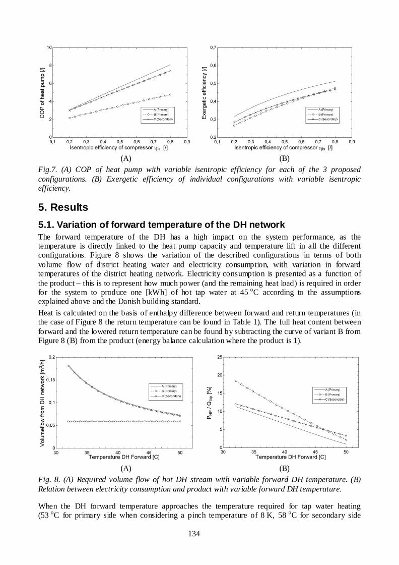
134

(A) (B) Fig.7. (A) COP of heat pump with variable isentropic efficiency for each of the 3 proposed configurations. (B) Exergetic efficiency of individual configurations with variable isentropic efficiency.

5. Results 5.1. Variation of forward temperature of the DH network The forward temperature of the DH has a high impact on the system performance, as the temperature is directly linked to the heat pump capacity and temperature lift in all the different configurations. Figure 8 shows the variation of the described configurations in terms of both volume flow of district heating water and electricity consumption, with variation in forward temperatures of the district heating network. Electricity consumption is presented as a function of the product – this is to represent how much power (and the remaining heat load) is required in order for the system to produce one [kWh] of hot tap water at 45 oC according to the assumptions explained above and the Danish building standard. Heat is calculated on the basis of enthalpy difference between forward and return temperatures (in the case of Figure 8 the return temperature can be found in Table 1). The full heat content between forward and the lowered return temperature can be found by subtracting the curve of variant B from Figure 8 (B) from the product (energy balance calculation where the product is 1).

(A) (B) Fig. 8. (A) Required volume flow of hot DH stream with variable forward DH temperature. (B) Relation between electricity consumption and product with variable forward DH temperature.

When the DH forward temperature approaches the temperature required for tap water heating (53 oC for primary side when considering a pinch temperature of 8 K, 58 oC for secondary side

135

according to the assumptions of Table 1), the consumption of electricity is reduced significantly; while almost the full energy flow is required from the district heating network. This is due to the significantly reduced thermal load in each of the heat pump configurations. As discussed above, configuration C has a slightly higher condenser load as in variant A, thus increasing the electricity consumption for the heat pump correspondingly at all temperature levels.

5.2. Variation of return temperature of the DH network Changes in return temperatures are highly important, as not only the electricity consumption of the heat pump booster configuration is affected, but also the temperature difference between the forward and return of the district heating network. Thus the optimal heat pump must perform with high efficiency in a range of high temperature differences between forward and return temperatures. Assuming tap water at 10 oC, and a finite heat exchanger (8 K), 18 oC is the lowest reachable temperature for the return water in the district heat system by direct heat exchange. Lower temperatures can only be achieved by using the heat pump evaporator to cool the stream further, which in this study only is considered in variant B. With an increase in return temperature of the district heating network, power consumption is reduced as the evaporation temperature of the heat pump refrigerant can be increased. An evaluation of the heat pump characteristics with a change in return temperature is considered in Figure 9 (constant forward temperature corresponding to Table 1). From the curvature of variant A and C in Figure 9 (B) it is clear that an optimum exists if the district heating water from Figure 9 (A) has a change in value.

(A) (B) Fig. 9. (A) Required volume flow of hot DH stream with variable forward DH temperature. (B) Relation between electricity consumption and product with variable return DH temperature

The differences between configurations A and C are quite hard to spot in Figure 9. In principle it does not make sense to display variant B, as the return temperature of the DH network is not controlled. The visible changes in Figure 9 (A) correspond to the previously addressed wish to show the differences in flow of DH water required to fulfil the tapping process.

5.3. Comparison of results using exergy

Exergy is used as another way to evaluate the performance of the different concepts. In this evaluation the different temperature levels of the district heating network is evaluated. Exergy is furthermore a good evaluation parameter when more than one fuel stream combine into only one product, as optimum between the different fuel streams is easily spotted. The lower electricity consumption of configuration A is rewarded in the calculation of exergetic efficiency throughout the entire range of forward and return temperatures considered in the paper. Considering the initial calculations, and the sensitivity study of heat exchanger performance and

136

isentropic efficiency, the distribution between the performances of the individual configurations is distinct. Figure 10 shows the exergetic efficiency of the three different variants, considering both the forward and the return temperatures. From Figure 10 (B) it seems that the second law efficiency is not improved with a return temperature above 25 oC in either of the cases, because the trade-off between reductions in electricity consumption is no longer compensating the increased exergy content of the heat consumption. The influence of pressure losses on exergy destruction is not considered in the systems and would lower efficiency further at the higher temperature due to higher flow rates. Increasing the forward temperature seems to be beneficial to the point where heat pump is no longer needed in the system. This is further discussed in section 6.

(A) (B)

Fig. 10. (A) Exergetic efficiency of individual configurations with variable DH forward temperature. (B) Exergetic efficiency of individual configurations with variable DH return temperature.

Variant B performs well with a low temperature return stream, or very high forward temperatures. Allowing this configuration additional heat from the space heating as proposed in section 4.2 might improve the performance of the configuration considerably, but in the temperature regime proposed in the above calculations, the configuration is not advantageous in any part of the temperature span considered.

5.4. Constant temperature difference between forward and return

As it is not easy to find the optimal forward temperature from the above calculations, an additional calculation has been performed with a constant temperature difference (18 K) between forward and return of the district heating network. This is to rule out the coinciding effects of very high temperature lifts in the heat pump in one end and high thermal heat pump load in the other end of the studied temperature range.

In figure 11, most of the range is clearly covered by the configuration A. Only at very high temperature levels configuration B is advantageous. The secondary system C is inferior in the entire range.

137

Fig. 11. Exergetic efficiency of the individual configurations with constant temperature difference between forward and return line of the district heating network.

6. Discussion Several system configurations have been considered in the initial work of the project based on forward and return temperatures corresponding to table 1. Of the investigated systems, the three configurations presented in this paper have provided the best performance. It is not unlikely that other energy efficient solutions can exist. The three variants have been chosen based on the criteria considered in the overall project, not only to satisfy energy efficiency, but also to comply with e.g., state of the art technology and DH network considerations. Considering both Fig. 8 and Fig. 10 (A), the optimal operation temperature of the district heating forward is not easily determined. The method used in fig. 11 show, that with a reasonable temperature difference throughout the range (18 K), the thermal load is the important factor to observe, as the COP is (almost) constant. Determination of optimal forward temperature of a low temperature district heating network will therefore not depend on the heat pump booster unit, but rather on external factors such as heat loses in the distribution network, sustainable sources and optimum production criteria for the combined heat and power plant. This effect is also shown in In Fig. 10 (B), as the exergetic efficiency levels out without consideration to the improvement in COP from increasing the evaporator temperature. From the same figure it is clear, that with a constant forward temperature (40 oC), the return temperature has an optimum (25 oC – 30 oC), which presumably would not be beneficial for the remaining network. Consulting Figure 10 (A) it is clear that the exergetic efficiency decreases with consumption of electricity in the heat pump configurations. When approaching the temperatures where direct heat exchange is possible, the exergetic efficiency increases, as heat losses are not considered in the network. If the heat pump booster unit is used in a system where it is coupled with a traditional district heating network, changes in the heat and power prices can be neglected. The reason for this is that the new system does not significantly change the operating conditions of the combined heat and power plant or the capacity of the transmission line in the district heating network. In this case only the heat losses in the novel DH system, and the increased end user capacity of the DH system from using lower temperatures can be compared with the additional electricity consumption.

7. Conclusion Three heat pump schemes were singled out for evaluation in a low temperature district heating network in order to increase tap water temperature to meet the Danish standard. Out of the three

138

heat pumps, two are used to boost the network temperature prior to heat exchange with the tap water, while the third is used to boost the temperature of the heated tap water. Variant A was found to be the most efficient configuration in the temperature range considered. In the expected temperature range the heat pump has an exergetic efficiency between 0.4 [/] and 0.6 [/]. Variant B proved that power consumption might not become significantly increased, if the heat pump is used to actively lover the temperature of the return flow as source heat. This would allow for lower flow rates to meet the tap water requirements.

Acknowledgments This work was supported by the Danish Energy Technology Development and Demonstration Programme (EUDP).

Nomenclature Time rate of exergy, kW

h Enthalpy, kJ/kg .

m Mass flow rate, kg/s p Pressure, kPa P Electricity, kW Q Heat, kW s Entropy, kJ/(kg*K) t Temperature, C

Volume flow rate, m3/h subscripts 0 Dead state i Index (component) DH District heating network

References [1] Thorsen J E, Christiansen C H, Brand M, Olesen P K, Larsen C T. Experiences on Low-

Temperature District Heating in Lystrup – Denmark. Procedings of International Conference on District Energy 2011, Slovenia.

[2] Bøhm B, Danig P O. Monitoring the energy consumption in a district heated apartment building in Copenhagen, with specific interest in the thermodynamic performance. Energy and Buildings 2004; 36; 229 – 236

[3] Elmegaard B, Houbak N. Simulation of the Avedøreværket Unit 1 Cogeneration Plant with DNA. Proceedings of The 16th International Conference on Efficiency, Cost, Optimization, Simulation, and Environmental Impact of Energy Systems 2003; 1659-1666

[4] Asada H, Boelman EC. Exergy analysis of a low temperature radiant heating system. Building Services Engineering Research & Technology 2004; 25 (3); 197-209

[5] Danish Standards. Code of Practise for domestic water supply installations (DS 439). 2009; Fourth edition.

[6] Engineering Equation Solver (EES). 2011 F-Chart Software, LLC. http://www.fchart.com/ees/ [accessed 20.01.2012]

[7] Nellis G., Klein S A. Heat Transfer. Cambridge university press, NY. 2008. ISBN 978-0-521-88107-4.

139

[8] Bejan A, Tsatsaronis G, Moran M. Thermal Design and Optimization. Wiley, NY. 1996 ISBN 978-0-471-58467-4 [9] Rosen M A, Dincer I. Effect of varying dead state properties on energy and exergy analyses of

thermal systems. Int J Therm Sci 2004; 43: 121–133



140

Exergoeconomic Diagnosis: a Thermocharacterization Method by Irreversibility

Analysis

Olivares-Arriaga A.a, Zaleta-Aguilar Ab, Rangel-Hernández V. H.c and Belmán-Flores J. M.d

a University of Guanajuato, Salamanca, Gto., México, [email protected] , b [email protected] ,c [email protected], d [email protected]

Abstract:

The paper at hand proposes an exergoeconomic diagnosis based upon the irreversibility characterization of the components by setting up the Rerefence Operating State (ROS) of the thermal power plant. The diagnosis introduces a new parameter, B, which represents the total irreversibilites attained to a subsystem or component at either design or off-design conditions (either partial or full loads). The elementary characterization of the reference state permits to detect changes on irreversibilities due to intrinsic or induced malfunctions. Reliability of the method is proven by its application to an actual Combined Power Plant. Data is obtained by means of software and hardware installed in the power plant. This has pemitted to obtaining a real-time exergoecomic diagnosis. Results from the study have been useful to detect the deviations in the thermal regime in terms of the irreversibilities of the components.

Keywords: Irreversibility, Exergo-characterization, Diagnosis.

1. Introduction The main idea of a thermoeconomic diagnosis is to pinpoint malfunctions into the components of a system as well as to quantify the additional consumption of resources because of them. The need to improve thermal processes have led to researchers to propose different methodologies for thermoeconomic diagnosis. Valero et. al. proposed the Exergy Cost Theory, which consisted in indentifying the causes and assessing their impact on additional consumption (i.e. Fuel Impact). However, the method required to be applied at constant power output. A first formulation to determine the causes of irreversibilities was proposed by Valero and Lozano et. al.[1]

i

*T PF k I j ,

this formulation relates the exergetic costs of each component, changes of irreversibilities to find the change in resources. An alternative formula was presented by Lozano and Valero [2]

*T P PF k

j j , however, this formulation does not consider changes in the local products of each component. Reini, Lazzaretto, and Macor [3] developed a new formulation to calculate the impact to Fuel.

j i i

n n n* *

T P 0 ji i 0 P 0 si 1 j 0 i 1

F k x P x k x P (1)

This equation allows finding the contribution of each component to the final variation of resources. One of the main problems of exergoeconmic formulation is that it takes to get all the exergy of both reference state and test state of all the components and perform complex matrix formulations. The philosophy of these methods is to compare the actual operating conditions with the reference operating conditions, maintaining the product (power) of the plant and environmental conditions constant.

141

The main disadvantage of these methods is that it requires complex calculations so it is necessary to have expensive software and hardware. Zaleta [4], proposes to make the diagnosis through of a thermodynamic simulation based on the first and second laws of thermodynamics. The methodology is able to analyze the changes produced by malfunctions in two global indicators of the thermodynamic cycle: the total power produced and the thermal regime (inverse of efficiency). This is based on a comparison between two operating conditions, a condition is the test operation (COP) which reflects the current operating conditions, and the other is the reference operating condition (COR) which can be taken in thermal balance or acceptance testing, it also uses energy and exergy analysis for the evaluation of the thermal regime and the total power generated; which are the most appropriate indicators to indicate the operation of a power plant. This diagnostic method has been used in actual power plants, where several malfunctions and external variations are common during operation and are detected in real time. The series of papers, Tadeus, presented by Valero compiled the evolution of different kinds of diagnostic methods. The complexity of the mathematical formulations and solution arrays, the high degree of instrumentation in the overall process (which is affected when there is no energy balances), the low accuracy of the results and the lack of understanding and comprension of the results by plant operators. The thermo-characterization theory proposed by Zaleta (2009) aims to diagnose each component in isolation on the impact of anomalies and using formulas to determine the overall effect on the process. The methodology of this theory was validated with the Method of Reconciliation and the results yielded a percentage relative error less than 5%. However, this new thermo-characterization theory considers not simultaneously enthalpy and entropy changes; therefore, two analysis most performed to find the change in the thermal regime first with respect to variation of the parameter and other with respect to the parameter . In this paper we set out again the premises of the theory of thermo-characterization but based on exergy analysis. This new approach considers variations of the parameters and in a new single parameter .

2. Diagnosis theory based on exergy thermo-characterization Premise 1: Distribution of an energy system and local processes. All advanced energy system can be subdivided into n isolated subsystems, delimited by a control volume with strategically defined boundaries according to the instrumentation, process sections, etc. Figure 1, Shows the disaggregation of an open Brayton cycle.

Fig. 1. Gas turbine cycle with subsystems (n=4 components) and (p=8) estrategy points.

142

Each control volume comply the mass and energy balances. Changes in thermodynamic conditions of input and output of the mass flow rates in each component i, during a process (heating, cooling, work, reaction, etc.), can be characterized by the parameters ( i, i, i, FR) applied according to the control volume and the properties of defined mass flux, shown in the figure 2. Therefore, (4) describes the changes in the parameter j and (5) defines the mass flow ratio.

Fig. 2. Volume of control of i-th component.

The parameter i is calculated from the enthalpy difference between the input minus output enthalpies.

, ,1 1

n m

i e s i e i j s ji j

kJ h h x h y hkg

(2)

where: 2

2estaticach h gz x

,, ; s je i

i je s

mmx y

m m The difference of entropy is determinate with the next equation:

, ,1 1

n m

i e s i e i j s ji i

kJ s s x s y skg K

(3)

The parameter i refers to the difference between the flows of inlet and outlet exergy, this is calculated from the parameters i, i and the chemical exergy.

01 1

, , 0 , ,1 1 1 1 1 1

n m

i i ji i

n m n m n m

i e i j s j i e i j s j i ji

Q Qi i s e

Q Qs e

i i i i i

kJ T x yk

e eg

x h y h T y ex s y es x (4)

The relationship between the actual mass or volume flow regarding to the design indicates the load which is operating the thermal cycle.

reftest

ref

test

pvm

FRpm

v (5)

Premise 2: State of reference to different loads and modes of operation. An energy system is designed to operate at different loads depending on energy demand. The adjustment of the load control systems have been used in the admission of the working fluid, regulation of IGV (Inlet Guide Vane) for gas turbine or control valves for steam turbines. Load change (FR) produces changes in power, is well known that the power generated is directly proportional to the mass flow used to produce, in addition the properties change; however, these can be calculated for each load

143

from the parameters . If malfunctions are not considered in the exergy balance of the components, these parameters calculated allow us to establish the reference state of i-th component, i.e. we will know the trajectory in two-dimensional space ( , P) of the component. The reference state is calculated from the heat balances provided by the manufacturer and / or performance testing and thermodynamic simulator. Figure 3a shows the reference trajectory to be followed by the component in space , P). values can be characterized (using polynomial regression) as a function of P.

(a) (b)

Fig. 3. a) Trajectory of reference State, b)Effect of the j-th malfunction on the i-th parameter.

Premise 3: Effect of malfunctions or anomalies. Figure 3b shows the effect of a malfunction. The point "R" is the reference point that component should be presented for current load if there not were any anomalies. The vectors in the plane ( , P) are the deviations in the parameters due to the malfunction. The malfunctions can be selected by the criterion of the designers, operators, or by free variables of a thermodynamic simulation of the plant as proposed Zaleta [4]. These variables can be classified into three categories of m variables:

a) Environmental (P0, T0, HR, HHV, etc.) b) Control and set Point (IGV, T, , etc.) c) Internal Indicators ( iso, UA, etc.)

If there would be more than a malfunction, these would always be in the same plane and their overall effect will be equal to the vector sum of each of the malfunctions. To find the parameter variations in function of each of the possible malfunctions applies the concept of the derivation of these parameters in relation to each malfunction. Mathematically:

0i i iT

Malf Malf Malf (6) We may establish a matrix of malfunctions which represents the variation of the parameter for each component with respect to each possible malfunctions. To find each term within the matrix is necessary to use a simulator that allows us to independently vary each of the malfunctions and to find the effect of these variations in the parameter . It should be noted that the matrix of malfunctions correspond to a single power (P), however, we can obtain these matrices to principal workloads: VWO (Valve wide open), 100%, 75%, 50% and 25%.

1

1 1

1

n

n m FR

n

m m

Malf MalfMalf

Malf Malf (7)

144

As mentioned in the previous paragraph we can determine the variation of with respect to each malfunction and to different loads, then it can be said that the variation of is a function of the malfunctions and workload.

,ij

j

f P MalfMalf (8)

Premise 4: Test performance. There are rules or procedures for conducting performance tests to energy systems such as performance tests codes (PTC) of the ASME. For testing is necessary to install strategically local instrumentation points (p) to find the basic thermodynamic properties (such as p, T, m , Q, etc..). The main objective of performance testing is to obtain the current values of:

I. P II. ,j testMalf y ,j ref cteMalf Malf P

III. , ,j j test j refMalf Malf Malf IV. ,i test

V. ,i ref P VI. , ,i i test i ref

VII. ref P y refRT RT P VIII. test ref y test refRT RT RT

Premise 5: Reconciliation of local malfunctions. Deviations found in each thermo-characterización parameter i by specific test performance can be disaggregated as the effect of malfunctions Malfj, this is the total effect of each of the malfunctions. Equation (9) shows this variation:

,

,

,1 ,1

j act

j ref

Malfmi

i i i m jj jMalf FR

dMalfMalf

(9) For n components, the reconciliation of malfunctions is represented as the sum of all deviations of the parameter:

1 1n n m mMalf dMalf (10)

Premise 6: Global Impact. Global parameters of a plant are function on the characteristics of the equipment and the parameters of each component. Using a simulator of the plant, the efficiency ( ) or thermal regime RT (inverse of the efficiency) are a function of the parameters and of the workload P, (11), (12).

1 , , , ,j mf P (11)

1 , , , ,j mRT f P (12)

Any variation in the parameters will indicate that there is a malfunction that can be characterized by the impact on global parameters and RT in a vector of dimensions 1m , (13) y (14):

1

, , , ,i j mP PP (13)

1

, , , ,i j mP PP

RT RT RT RT

(14)

145

From the information of the performance test we find deviations in the global indicators; however, we do not know which malfunctions are presented and their impact in these parameters. To determine the effect of each malfunction in these global parameters, we can apply the method of reconciliation [6]. However, as we only have the variations of the parameters as effect of malfunctions a modification must be made to the method of reconciliation (chain rule for total derivation) that is:

,

,1 1

j test

j ref

Malfn miT

ji j i jMalf P

dMalfMalf

(15) ,

,1 1

j test

j ref

Malfn miT

ji j i jMalf P

RTRT dMalfMalf

(16) The above equations represent the change in the global parameters of the plant as function to local variations of the parameters of each component. These variations of the parameters are in turn the effect of the plant malfunctions presented in.

3. Implementation of the exergo-characterization to a 420 MW combined cycle

The culmination of each new theory is to find the energy assessment of this application in real cases. This paper will talk about the use of make use of the exergo-characterization to find deviations from the thermal regime of a combined cycle operation. As a first step in the application describes the main features of the combined cycle components are described to be analyzed and then follow the application of the methodology or assumptions presented in the previous paragraph. Only the exergy balances for the components is shown , but to create the reference state and test state was performed in the program EES (Engineering Equation Solver®) which considers mass balances, energy and exergy.

Fig. 6. Scheme of the real combined cycle.

146

3.1. Description of the combined cycle The case of study of this work is referred to a combined cycle (Figure 6) consisting of a gas turbine of 128.98 MW Westinghouse with an efficiency of 34.8%, a Siemens gas turbine of 131.59 MW with an efficiency of 34.74% and a steam turbine ABB-Alstom with a capacity of 127.67 MW and an efficiency of 33.03%, data from a performance test conducted in January 2004 by staff of the Laboratory test Equipment and Materials (LAPEM). Figure 6 shows the entire outline of the combined cycle that serves as a guide for the identification of the main equipment and flows in which the plant is discretized. Each has a tag number that identifies itself. Given the level of detail, the whole scheme is divided, in order of appearance in gas turbines, heat recovery, steam turbine and the air condenser. Flows definition. In Table 1 all flows are systematically identified (exchange of mass and energy) of the combined cycle. It helps in the interpretation of the cycle scheme. The numbering of the flows and their interaction with each of the equipment in the plant, we propose a logic numeration according to the start of the cycle, i.e. cycle gas, putting a zero in this cycle for their distinction and avoid some confusion with vapor cycle, and so on until the end of it in the air cooled condenser.

3.2. Implementation of the premises of the exergo-characterization Premise 1. Disaggregation of energy system and its local processes. In this case of study, the combined cycle was divided into 17 major components (n = 17) each delimited by its volume control. In the scheme of the combined cycle, likewise settled 32 points of interaction between the different volumes of control (p = 32). For each control volume are established mass and energy balances. Table 1 shows the values of the design parameters (FR = 1) of all the 32 points defined in the cycle. Table 2 shows the major components that form the thermodynamic cycle. Premise 2. Reference state at different loads and modes of operation. As mentioned thermodynamic cycles are designed to work at different loads in the case of gas turbines, this is achieved decreasing the inlet compressor area by operating the IGV's. By reducing the inlet area decreases the mass flow and hence the power of the gas cycle. Using a thermodynamic simulator performed in software and data based on the design of components and design heat balances and / or acceptance testing is possible to vary the value of the IGV to find the variation of the parameters

, and as a function of the load P without abnormalities (reference state). Figure 4 shows the variation of the parameter as a function of the load P, it should be noted that this parameter relates the enthalpy and entropy changes into one. For each component reference graphs must be calculated considering that the load P of each component will vary depending on the percentage of power. Premise 3. Effects of malfunctions or anomalies. In order to understand the perturbation and effect of different anomalies or malfunctions on the reference state of each n component is necessary two steps:

I. Definition of malfunctions or anomalies. II. Analysis of the perturbation by effects of each of the anomalies in each of the components.

Definition of malfunctions or system failures. The definition of m free variables of the system is necessary. Each variable corresponds to each possible malfunctions that may occur in the system. These variables should be chosen based on experience of the analyzer; Table 3 shows the variables and the corresponding description of malfunctions for the combined cycle. Analysis of the perturbation of malfunctions on the reference state of the n sub-systems. Once identified malfunctions or anomalies in the whole system, the next step is to calculate the variation of the parameter with respect to each of the malfunctions to the different load levels.

147

Table 1. Description of conditions in the combined cycle

TAG Description T

[ºC] p

[bar] h

[kJ/kg] s

[kJ/kgK]

[kg/s]

b [kJ/kg]

W [MW]

Gas Turbine (Units 5 & 6)

00 Environment Conditions 20 0.8077 20.20 0.07136 0

015 Air Compressor suction 20 0.79 20.20 0.07136 285.49 0

025 compressor discharge 381.1 9.29 392.33 0.8956 285.49 130.51

035 Fuel Flo w Combustion Chamber 47134.4 7.864 0

045 Combustion gases at the inlet to turbine 1238 9.11 1620.12 1.459 293.35 1193.11

055 Discharge of the combustion gases in the gas turbine 656.96 0.83 809.24 1.552 293.5 355.07

065 Chimney flue gas 125.3 0.8077 144.70 0.5079 293.5 -3.47

WC5 Power consumed by the compressor 106.24

WG5 Power developed by the turbine 237.87

016 Air Compressor suction 20 0.80 20.20 0.07135 331.3 0.00001

026 compressor discharge 399.34 10.45 411.84 0.9250 331.3 141.40

036 Fuel Flo w Combustion Chamber 47134.4 8.328

046 Combustion gases at the inlet to turbine 1191 10.24 1534 1.358 339.62 1137.0

056 Discharge of the combustion gases in the gas turbine 612.38 0.83 742.33 1.470 339.62 312.02

066 Chimney flue gas 120.0 0.8077 138.56 0.4924 339.62 -5.07

WC6 Power consumed by the compressor 129.75

WG6 Power developed by the turbine 269.01

Heat Recovery Steam Generator (HRSG 1 & 2) – Steam Turbine

1 Principal steam 548 115 3481.66 6.6736 79.35 1528.23

2 Hot Reheat steam 548 20.02 3574.52 7.5667 97.96 1359.25

3 Cold Reheat Steam 327.91 22.82 3081.27 6.8079 77.63 1088.47

4 Outlet Steam from Intermediate Pressure Steam Turbine 301.46 3.51 3071.30 7.6342 99.36 836.24

45 Inlet Steam to Low Pressure Steam Turbine 294.55 3.48 3057.25 7.6143 108.24 828.04

5 Outlet Low Pressure Steam from HRSG 217.20 3.5 2898.7 8.8602 8.86 759.05

6 Exhaust Steam outlet from LPST 41.51 0.08 2427.68 7.7553 108.44 157.14

61 Suction water of principal pump 137.8 3.40 579.9 1.717 97.32 86.81

60M Discharge Intermediate Pressure water of principal pump 137.9 22.30 581.6 1.718 77.59 88.73

60A Discharge High Pressure water of principal pump 138.4 115 589.5 1.721 19.732 98.09

71 Suction water of condensate pump 41.51 0.08 173.84 0.5925 108.44 3.07

70 Discharge water of condensate pump 41.62 15.45 175.66 0.5934 108.44 4.64

Electric Generator

WNETA Power net 404.96

WBC Power to condensate pump 0.1977

WBA Power to principal pump 5.3211

WAUX Power to auxiliary equipment 6.320

148

Table 2. Principal components in the thermodynamic cycle

Equipment Integration in the cycle

I Filters Gas Cycle 5 II Compressor Gas Cycle 5 III Combustor Gas Cycle 5 IV Drive turbine Gas Cycle 5 V HRSG Gas Cycle 5 – Steam cycle VI Principal pump Gas Cycle 5 – Steam cycle VII Filters Gas Cycle 6 VIII Compressor Gas Cycle 6 IX Combustor Gas Cycle 6 X Drive turbine Gas Cycle 6 XI HRSG Gas Cycle 6 – Steam cycle XII Principal pump Gas Cycle 6 – Steam cycle XIII High Pressure Turbine Steam cycle XIV Intermediate Pressure Turbine Steam cycle XV Low Pressure Turbine Steam cycle XVI Condensate pump Steam cycle XVII Air cooled condenser Steam cycle

Fig. 4. Effect of the j-th malfunction on i-th parameter.

The variance of each parameter depends on each of malfunctions; in the present case we have 20.

1 1 11 1 2 20

1 2 20

dMalf dMalf dMalfMalf Malf Malf (17)

for each component we find in similar form the parameter variation as a function of all malfunctions. Premise 4. Performance test of a generating plant can be performed using the procedures provided by the test codes (PTC' s). To determine the reference state of the combined cycle was a performed

149

simulator which reproduces the design conditions that each flow has in the cycle and efficiencies of the main components.

Table 3. Definition of malfunctions with their reference and test values Malfunction Variable Description Test

value Reference

value Difference

Malf1 DPF1[%] Drop Pressure in Filters – Gas Turbine 5 3.02 2 1.02 Malf2 comp,1[%] Efficiency of compressor – Gas Turbine 5 79.3 80.74 -1.44 Malf3 exp,1[%] Efficiency of turb ine – Gas Turb ine 5 85.733 87.67 -1.937 Malf4 DPC1[%] Drop Pressure in combustor – Gas Turbine 5 3.5 2 0.015 Malf5 TIT1[°C] Temperature Inlet to Turb ine – Gas Turb ine 5 1185 1200 -15

Malf6 DPHRSG,1 [mmH2O]

Drop Pressure in HRSG side Gases – Gas Turbine 5

330 230 100

Malf7 DPF2[%] Drop Pressure in Filters – Gas Turbine 6 2.5 1.5 1 Malf8 comp,2[%] Efficiency of compressor – Gas Turbine 6 80.36 81.58 -1.22 Malf9 exp,2[%] Efficiency of turb ine – Gas Turb ine 6 86.425 87.05 -0.625 Malf10 DPC2[%] Drop Pressure in combustor – Gas Turbine 6 5.2 2 3.2 Malf11 TIT2[°C] Temperature Inlet to Turb ine – Gas Turb ine 6 1205 1200 5

Malf12 DPHRSG,2 [mmH2O]

Drop Pressure in HRSG side Gases – Gas Turbine 6 506.61 230 170.61

Malf13 THP[%] Efficiency of High Pressure Turbine 81.87 83.58 -1.71 Malf14 TIP[%] Efficiency of Intermediate Pressure Turbine 91.52 92.95 -1.43 Malf15 TLP[%] Efficiency of Low Pressure Turbine 92.96 93.39 -0.43

Malf16 Pvacuum [bara] Vacuum Pressure in condenser 0.086 0.08 0.006

Malf17 P1[bara] Pressure of Principal Steam to HPST 115.5 115 0.5 Malf18 T1[°C] Temperature o f Principal Steam to HPST 549.4 548 1.4 Malf19 T2[°C] Temperature of Reheat Steam to IPST 550.3 548 2.3

Malf20 T5[°C] Temperature o f Steam to Low Pressure Steam Turbine

219.3 217.2 2.1

Wnet[MW] Power Net 372.5 380.75 -8.25

One of the requirements to know the actual or test operation of the plant is to know the implementation details of the important points of the cycle. The combined cycle plant has a distributed control system and an OPC (OLE for process control) that communicates with the control to extract data from the instrumentation. The data obtained from the operation malfunctions of the plant are summarized in Table 3. Premise 5. The deviations found for each specific test performance in exergo-parameter characterization i can be disaggregated as the effect of the 20 malfunctions Malfj, this is the total effect of each of the malfunctions in the first component.

1 1,1 1,2 1,20372,5P MW (18) similarly we found the deviations of each parameter . Table 4 shows the effects that each malfunctions produces in the parameters i corresponding to each principal component in the combined cycle. This table shows that there are malfunctions that affect the operation of equipment even if this is present on equipment; these malfunctions are known as induced malfunctions. It is also noticed that there are components which are not affected by all malfunctions

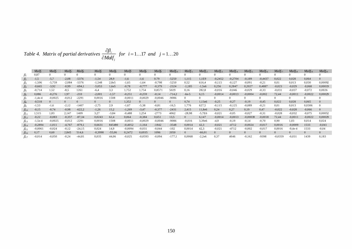
150

Table 4. Matrix of partial derivatives i

jMalf for 1 17i and 1 20j

Malf1 Malf2 Malf3 Malf4 Malf5 Malf6 Malf7 Malf8 Malf9 Malf10 Malf11 Malf12 Malf13 Malf14 Malf15 Malf16 Malf17 Malf18 Malf19 Malf20

1 0,87 0 0 0 0 0 0 0 0 0 0 0 0 0 0 0 0 0 0 0

2 -1,5 -5,7 -2,08 -5376 -1,54 28,9 -1,6 -1,6 0.79 -5250 1,115 1,1E9 -0,2452 -0,2704 -0,189 -0,4437 0,022 0,028 0,064 0 3 -1,506 -5,759 -2,084 -5376 -1,548 2,8e5 -1,65 -1,64 -0,798 -5250 0,52 616,4 -0,115 -0,127 -0,091 -0,21 0,01 0,013 0,030 0,00092 4 -0,665 -3,92 -0,99 -694,1 -5,053 1,6e5 -0,78 -0,777 -0,379 -2324 -1,185 -1,5e6 0,256 0,2847 0,2027 0,4887 -0,023 -0,029 -0,068 0,00019 5 -0,714 1,52 -8,5 1261 -6,4 3,3 1,752 1,754 0,8571 5029 0,16 282,8 -0,016 -0,046 -0,029 -0,33 -0,031 -0,037 -0,072 0,0026

6 0,086 -0,276 1,97 -210 -2,001 -1,57 -0,251 -0,259 -0,14 -714,2 -6e-5 6,15 -0,0014 -0,0013 -0,0004 -0,002 72,44 -0,0011 -0,0022 0,00029 7 -1,4e-4 -0,0025 -0,012 -2291 0,0016 1508 -0,0011 -0,0029 -0,0046 -9086 0 0 0 0 0 0 0 0 0 0 8 -0,518 0 0 0 0 0 1,352 0 0 0 0,74 1,13e6 -0,25 -0,27 -0,19 -0,45 0,022 0,028 0,065 0 9 -1,53 -1,6 -2,12 -1407 -2,75 2,9 -1,67 -5,38 -0,81 -16,5 1,776 627,5 -0,115 -0,125 -0,089 -0,21 0,01 0,013 0,0306 0

10 -0,15 -0,74 -0,98 -622,2 -1,26 15,2 -1,269 -3,47 -0,377 -2431 2,415 11,8e6 0,24 0,27 0,19 0,47 -0,022 -0,028 -0,066 0 11 1,515 1,83 2,147 1409 3,27 -3,84 -0,488 1,254 -2773 4062 -28,98 -5,7E6 -0,021 -0,05 -0,027 -0,31 -0,028 -0,032 -0,075 0,00052 12 -0,22 -0,083 -0,357 -87,34 0,0243 62,4 0,064 -0,384 0,651 13,5 0 6,147 -0,0014 -0,0013 -0,00039 -0,0018 72,44 -0,0011 -0,0022 0,00029 13 -1,5e-4 -0,0025 -0,012 -2291 0,0016 1508 -0,0011 -0,0029 -0,0046 -9086 -0,016 3,39e6 -4,9 -0,19 -0,14 -0,70 0,90 1,03 0,014 0,024

14 -0,2894 -1,011 -4,767 -879,1 0,6631 845490 -0,4052 -1,164 -1842 -3548 0,0014 42,3 -0,021 -4712 -0,0024 -0,017 0,0016 -0,0009 1533 -0,041 15 -0,0061 -0,024 -0,12 -24,15 0,024 14,9 -0,0094 -0,031 -0,044 -102 0,0014 42,3 -0,021 -4712 -0,002 -0,017 0,0016 -9,4e-4 1533 -0,04 16 0,17 0,60 2,845 514,6 -0,3998 -55,06 0,2472 0,6935 1096 2050 0 -66,01 0 0 0 0 0 0 0 0

17 -0,014 -0,050 -0,24 -44,81 0,035 44,06 -0,025 -0,0593 -0,094 -177,1 0,0068 -2,2e6 0,37 4046 -0,162 -9398 -0,0359 -0,031 1439 0,183

151

3.3. Calculations for the deviation of the thermal regime of the combined cycle

Premise 6: Efficiency relationship by Second Law is:

o

i

BB (19)

or in terms of the thermal regime by Second Law is calculated as follows:

2 .1

nd Lawo

I LRT

B (20)

For calculating the deviations of each of the malfunctions to the thermal regime, it must be used the program of reference made in ESS to find optimum values that aims to show the thermodynamic cycle, ie the values that would have thermodynamic properties of the streams or efficiencies of the components if there were any malfunction. In addition, a test of the equipment is regarded with to evaluate the current condition of the plant. Once the evaluation of equipment is done a regulatory of regulatory procedures as well as the isentropic efficiency models and characteristic curves of the equipment can be considered.

Fig. 7. Grassman diagram of the combined cycle.

Figure 7 shows the Grassman diagram of the combined cycle, we see that the input exergy (exergy of fuel) had divided the two combustion chambers of the two gas turbines. The output of the hot gases from both gas turbine are introduced into the heat recovery (HRSG's) to produce steam for the Rankine cycle, eventually the gases are expelled to the atmosphere which represents the total loss of the combined cycle. Shown in this diagram the irreversibilities present in each cycle of the equipment. The air condenser uses electrical energy to move the fan for condensing the steam, however, this exergy comes from the same turbine after passing through the electric generator so

152

that there is no flow of exergy that is sent to the atmosphere for this reason exergy losses should only be the exergy that is lost in the flow gas of HRSG's. As example,

I. Compressor 1

Fig. 5. Exergy balance for compressor 1.

Figure 5 shows the exergy balance for compressor and the equations used to find the irreversibility. We found all exergy balances for each component in the cycle.

, 01,1 01,1 02,1 _1

, 01,1 _1

T II comp II

T II II comp II

I m b b W x L

I m W x L (21) where:

II IIx I I is the entropy loss generated in the compressor

L is the exergy loss in the flow gas to the output HRSG’s Finally, we found mathematical models of irreversibility on each component in function of the power and each malfunction. Below the equation for the steam turbine is only shown high pressure to illustrate their use in calculating the deviation of the thermal regime by Second Law.

1

2 021,

21 12468.05 7.933 8.221 0.00633 4.4776 10 0.0047

compXIII comp comp compI P P P (22)

The change in thermal regime must be equal to the change of the irreversibilities as defined by Second Law, that is:

,2 ,

1 1

1 T knd Law iP cte

k i i

IdRT dMalf

P Malf (23)

There is already a relationship between each irreversibility with respect to power and each malfunction, all the contributions can be calculated of each malfunction affecting each thermal cycling equipment, namely the variation of each irreversibility with respect to malfunctions. From the above definition it also follows that the sum of the changes in the total irreversibilities is the change thermal regime cycle. Equation (23) shows each contribution to the thermal regime based on the irreversibility of all components.

2 , 372 ,51.79266 5.11770 1.44992 7.15927 1.58317 0.00464 1.95410 5.37127

7.21231 4.17898 5.23907I II III IV V VI VII VIII

IX X X

nd Law PI I I I I I I I

I I I

dRT

0.00203 0.97790 1.23373 1.42685 0.00515 5.57756I XII XIII XIV XV XVI XVIII I I I I I

(24)

giving as total variation:

153

2 , 372,550.286nd Law P

dRT (25)

It is seen from equation (24) that the thermal regime is affected by intrinsic causes, i.e. which can be attributed to poor operation of the same components as well as induced malfunctions in a component where they are not presented but is affected by the change in properties at the entrance or exit in the component.

3. Conclusions The exergo-characterization includes in a single exergetic parameter the effect of malfunctions in the equipment that makes up a generation cycle. Also has been able to include the overall effect of each malfunction in the efficiency of the cycle or regime thermal as function of the irreversibility generated in the components of power cycles. As it has precision of a simulator, due the characterization performed in based on one, there are a good approximation of the effects produced by malfunctions regardless of the nature of them as it makes reference a simulator modeling with balances of First and Second Law. We show the exergo-characterization methodology applied on simple Gas turbine cycle developed in a practical way to understand your application. The methodology is applied to an advanced generation cycle. The application allowed knowing the deviation of the thermal regime by Second Law (inverse of the Second Law efficiency) as a function of the variation of irreversibility in each of the components of the combined cycle in consequence of the occurrence of malfunctions, seeing Table 4 and (24). However, it is necessary to have a cycle simulator to characterize in terms of exergy flow behavior of the cycle. Once you have completed this step only requires mathematical models generated for exergy parameters for diagnosis. For this reason, we can say that there is an improvement over the method of reconciliation that requires a simulator for the reconciliation of malfunctions every time you want to do the exergy assessment. Another improvement is that it has in terms of exergy evaluation of each component by itself or the entire cycle, the first as function of the parameters i and the second depending on the irreversibilities of each component.

Nomenclature b Exergy, kJ/kg B Exergy, kJ DPC Drop pressure combustor DPF Drop pressure filters e Exergy, kJ/kg F Fuel consumption, kW FR Mass flow ratio h Enthalpy, kJ/kg I Irreversibility, kW k Exergetic cost L Loss Exergy, kW

Mass rate, kg/s Malfuction

Thermal regime Temperature, °C

154

Turbine inlet temperature, °C x Reference values, mass fraction of inlet flow y Mass fraction of outlet flow W Power, MW Greek symbols Exergy difference Difference Efficiency Exergetic consumption Volume, m3/kg Entropy difference exergy efficiency Enthalpy difference

Subscripts and superscripts 0 Reference state comp Compressor i Inlet, i- th component iso Isentropic j j-th component o Outlet p Pressure , bar P Product Q Chemistry ref Reference load T Total test Actual load

References [1] Antonio Valero, M A Lozano, J A Alconchel, M Muñoz, and Cesar Torres. Guadeamo: A

system for energetic /exergetic optimization of coal power plants. ASME AES Vol 2-1, Computer-Aided Engineering of Energy Systems, Optimization, ed R.A. Gaggioli, ASME Book No. H0341 A, pp 43-49. New York, 1, 1986.

[2] Antonio Valero and M A Lozano. Application of the exergetic costs theory to a steam boiler in thermal generating station. AES Vol. 3-2 Analysis and Design of Advanced Energy Systems: Applications, eds. M. J. Moran, S.S. Steco, and G.M. Reistad, ASME Bokk No. G0377 B, pp 41-51. New York, 1987.

[3] M Reini, A Lazzareto, and A Macor. Average structural and marginal costs as result of a unified formulation of the thermoeconomic problem. Proceedings of Second Law Analysis of Energy System: Towards the 21st Century, Rome, 1995.

[4] Alejandro Zaleta, Armando Gallegos, and Victor Rangel. A reconciliation method based on a module simulator an approach to the diagnosis of energy system malfunctions. Int. J. Thermodynamics, Vol 7, No. 2. Pp 51-60, June 2004, ISSN 1301-9724, 2004.

[5] Vittorio Verda, Luis Serra, and Antonio Valero. Effects of the regulation system on the thermoeconomic diagnosis of a power plant part II: Application to a gas turbine- based

155

cogeneration plant. First International Conference on Applied Thermodynamics, ECOS 2001, July 4-6, 2001 ISTANBUL, 2001.

[6] A Toffolo and A Lazzaretto. On the thermodynamic approach to the diagnosis of energy system malfunctions indicators to diagnose malfunctions: Application of a new indicator for the location of causes. Int J. Thermodynamics, Vol. 7. No. 2, pp 41-49, June 2004, 2004.

[7] ASME PTC 6s 1988 (R 1995): Procedures for Routine Performance Tests of Steam Turbines. 1995.

[8] Alejandro Zaleta, Rosa Adriana Dominguez Vega, Abraham Olivares Arriaga, and Victor Hugo Rangel Hernandez. Thermoeconomic diagnosis theory based on thermocharacterization. Int. J. Thermodynamics, Vol 13, No. 4. Pp 143-152, 2010, ISSN 1301- 9724, 2010.

[9] D H Cooke. Modeling of off-design multistage turbine pressures by stodola´s ellipse. Energy Incorporated Pepser User´s Group Meeting Richmond, Virginia November 2-3, 1983.

[10] K C Cotton. Evaluating and Improving Steam Turbine Performance. ISBN 0-9639955-0-2, USA, 1998.

[11] T J Kotas. The exergy method of thermal plant analysis. Krieger Publishing, New York, 1995.

[12] A. Zaleta, H. Jimenez, J. Chavez, J. Pacheco, A. Campos, and A. Gallegos. Three statements for a reliable on-line thermoeconomic monitoring and diagnosis.dynamic reference state , acceptable performance tests, and the equalized reconciliation method. Proceedings of ECOS 2005, Trondheim, Norway June 20-25,2005, 2005.

[13] L. Correas. On the thermoeconomic approach to the diagnosis of energy system malfunctions suitability to real-time monitoring. Int.J.Thermodynamics,Vol.7,No.2,pp.85-84, June-2004, 2004.

[14] A. Zaleta, J. Royo, and A. Valero. Thermodynamics model of the loss factor applied to steam turbines. Int.J.Thermodynamics,Vol.4,No.3,pp.127-133,September-2001, 2001.

[15] J. Royo, A. Zaleta, and A. Valero. Analysis and evaluation of malfunctions in thermomechanical systems. AES.Vol.37,pp.103-108.ASME Book HO1126.1997, 1997.



156

Optimal Structural Design of Residential Cogeneration Systems Considering Their Operational Restrictions

Tetsuya Wakuia and Ryohei Yokoyamab a Department of Mechanical Engineering, Osaka Prefecture University

1-1 Gakuen-cho, Naka-ku, Sakai, Osaka 599-8531, Japan [email protected], CA

b Department of Mechanical Engineering, Osaka Prefecture University 1-1 Gakuen-cho, Naka-ku, Sakai, Osaka 599-8531, Japan

[email protected]

Abstract: An optimal structural design method of residential cogeneration systems considering various kinds of operational restrictions of system components is developed from the energy-saving viewpoint. The optimal structure of a residential cogeneration system, which consists of a cogeneration unit and its peripheral devices, is determined in considertation of multi-period operation, based on their operational restrictions, so that annual primary energy consumption may be minimized. The selection, operational restriction, and operation status of system components are expressed by binary variables, and input and output rates of energy flow, and stored energies of system components are expressed by continuous variables. As principal operational restrictions of cogeneration units without reverse power flow to commercial electric power systems, a constant power output operation, daily start–stop operation, and continuous operation are focused on. By formulating the relationship between the binary variables expressing the selection and those expressing operation status for system components, their selection and multi-period operation are simultaneously optimized. The formulated optimal structural design problem results in a mixed-integer linear programming problem. Moreover, the proposed method is applied to the structural design of a residential cogeneration system consisting of a cogeneration unit, whose candidates are a gas engine employing a constant power output operation, polymer electryte fuel cell empoying a daily start–stop operation, and solid oxide fuel cell employing a continuous operation, with a storage tank and gas-fired boiler, and peripheral devices, whose candidates are an electric water heater and air-cooled heat exchanger, for simulated energy demands. The results reveal that the selection of the cogeneration unit is influenced more by the generation and heat recovery efficiencies and the operational restrictions of the cogeneration units than by the consistency in the heat-to-power ratios of the cogeneration unit and energy demand.

Keywords: Cogeneration, Optimization, Structural design, Operational planning, Energy savings, Residential use.

1. Introduction Cogeneration applications to archive energy savings and cost reduction have been extended to ordinary residences due to the development of small-scale, high-performance energy-conversion machines, including gas engines, fuel cells, and Stirling engines. In Japan, a 1-kWe gas engine-based cogeneration unit (GE-CGS) [1] and 1-kWe class polymer electrolyte fuel cell-based cogeneration units (PEFC-CGSs) [2, 3] have been available for residential use. Recently, a 0.7-kWe solid oxide fuel cell-based cogeneration unit (SOFC-CGS) has been released [4]. These residential cogeneration units have differing heat-to-power supply ratios and operational restrictions. The GE-CGS has the highest heat-to-power supply ratio of the three types of residential cogeneration units; however, it must be operated under the constant power output in order to maintain a generation efficiency. PEFC-CGSs have higher generation efficiencies than the GE-CGS, and adopt a daily start–stop operation, in which they are started and stopped a maximum of once a day. This is because their performances are degraded by thermal cycling from operating temperature to a low temperature and back [5], and because input energy is required for start-up. The SOFC-CGS has the highest generation efficiency of the three types of residential cogeneration units; however, it must

157

be operated continuously because its high operating temperature requires a long warm-up time and high level of input energy. Moreover, in Japan, surplus electric power from residential cogeneration units cannot be transmitted to commercial electric power systems. Thus, they must be operated in response to variations in the electric power demand of individual residences; however, the PEFC-CGS and SOFC-CGS may have minimum electric power output because their generation efficiencies decline under partial- load conditions. Furthermore, residential cogeneration units require storage tanks to intermittently supply hot water. Hence, peripheral devices may be required, including an electric water heater to consume surplus electric power, an air-cooled heat exchanger to waste surplus hot water, and a gas-fired boiler to compensate for the shortage in the hot water supply. Combining plural peripheral devices with residential cogeneration units in accordance with various operational restrictions increases the flexibility of the optimal system structure; thus, a rational design of the residential cogeneration units and their peripheral devices for various energy demands is strictly required to archive energy savings and cost reduction. The benefits obtained by utilizing the three types of residential cogeneration units were previously analyzed. Paepe et al. [6] investigated the energy-saving effect of 4.7-kWe and 5.5-kWe GE-CGSs and a 4-kWe PEFC-CGS operated in a detached house and terraced family house in Belgium, through a whole-year simulation. Cockroft et al. [7] reported that a GE-CGS and SOFC-CGS meeting the maximum heat demand of typical residences in the United Kingdom needed to operate at a total utilization efficiency of more than 80% to achieve energy savings. Hawkes et al. [8] reported a cost-effective operation strategy for a 2-kWe GE-CGS and 2-kWe SOFC-CGS. Staffell et al. [9] developed a suitable operation strategy and cost target for a 1-kWe PEFC-CGS and 1-kWe SOFC-CGS in the United Kingdom, employing a Monte Carlo analysis. Dorer et al. [10] assessed the performance of a 4.7-kWe GE-CGS, 4.5-kWe PEFC-CGS, and 1-kWe SOFC-CGS under different power plant configurations in electric power systems, using a dynamic simulation model. In these previous studies, the residential cogeneration units could be operated flexibly to obtain the reported benefits because surplus electric power generated by them could be transmitted to commercial electric power systems. Some previous studies considered the constant power output operation of the GE-CGSs [6, 7] and continuous operation of the SOFC-CGSs [8, 10]; however, the daily start–stop operation of the PEFC-CGSs was not considered. Moreover, they did not attempt to optimize the system structure, comprising the cogeneration unit and its peripheral devices, for various energy demands. Yokoyama et al. [11] developed the optimal structure design method for large-scale energy supply systems, in which the selection and discrete capacity of system components were determined in consideration of their operations, using a mixed-integer linear programming approach. However, in this method, the input–output relationship of system components was formulated by single linear equations, and only their on-off status was considered as the operational restrictions. Against such a background, an optimal structural design method of residential cogeneration systems considering various kinds of operational restrictions of system components is developed from the energy-saving viewpoint. The optimal structure of a residential cogeneration system, which consists of a cogeneration unit and its peripheral devices, is determined in consideration of multi-period operation, based on their operational restrictions, so that annual primary energy consumption may be minimized; this means that the selection and multi-period operation of system components are simultaneously optimized. As principal operational restrictions of cogeneration units without reverse power flow to commercial electric power systems, a constant power output operation, daily start–stop operation, and continuous operation are focused on. Moreover, the variations in the generation and heat recovery efficiencies of cogeneration units under partial- load conditions were formulated using multiple linear equations. The proposed method is applied to the structural design of a residential cogeneration system consisting of a cogeneration unit, whose candidates are a GE-CGS employing the constant power output operation, PEFC-CGS employing the daily start–stop operation, and SOFC-CGS employing the continuous operation, with a storage tank and gas-fired boiler, and peripheral devices, whose candidates are an electric water heater and air-cooled heat exchanger, for simulated energy demands.

158

2. Optimal structural design of residential cogeneration systems

2.1. Summary of optimal structural design problem To consider seasonal and hourly changes in residential energy demands, a typical year is divided into M representative days; the index for the representative days is designated by m. Each representative day is divided into K sampling times, with a period of (i.e., = 24/K), and the index for the sampling times is designated by k. First, a superstructure for a residential cogeneration system is created; this consists of all the system components considered as candidates for selection and previously selected. Then, a real structure is created by selecting the system components from among the candidates [11]. The selected system components are operated in accordance with their operational restrictions and energy demands for each period. As a result, the selection and multi-period operation of the system components are simultaneously optimized so that annual primary energy consumption may be minimized. The operation of a residential cogeneration system with a storage tank cannot be determined independently at each sampling time; thus, a daily cyclic operation is considered, assuming that the energy demands change cyclically with a period of 24 h on each representative day; this means that the operation pattern of the selected system components is derived on each representative day.

2.2. Decision variables In this optimal structural design problem, the decision variables are classified into two types: design variables and operation variables. The selection of the system components is expressed by binary variables, classified as the design variables; the design variables do not depend on representative days and sampling times. For the operation variables, continuous variables are used to express the input and output rates of energy flow, and the stored energies of the system components at the kth sampling time on the mth representative day; and the operation status of the system components at the kth sampling time on the mth representative day is expressed by binary variables.

2.3. Constraints The constraints consist of the selection and performance characteristic in accordance with operational restriction of each system component, and energy balance relationships.

2.3.1. Selection of system components The selection of the system components is formulated using the design variables. As an example, a superstructure for the cogeneration unit, which has I candidates for the selection, is shown in Fig. 1. For any candidate, the input is the natural gas because fuel cell-based cogeneration units are driven by hydrogen reformed from natural gas in built- in fuel reformers; and the outputs are the electric

Fig. 1. Superstructure for selection of cogeneration unit.

159

power and hot water. Generally, one cogeneration unit is installed per single-family residence; thus, the constraint for the selection is formulated as follows:

(1)

where denotes the binary variable (design variable) expressing the selection of the ith candidate for the cogeneration unit. Equation (1) indicates the possibility that any cogeneration unit is not selected as the optimal system structure. This constraint can be applied to other system components, which are selected from multiple candidates.

2.3.2. Performance characteristic of system components considering their operational restrictions

The performance characteristic of candidates for the system components in accordance with their operational restrictions is formulated at each sampling time on each representative day. (a) Cogeneration units Some cogeneration units can be operated under partial- load conditions; however, the generation and heat recovery efficiencies depend on their load factors. Thus, the input–output relationship of the cogeneration units may have nonlinear characteristics, and it is modeled using multiple linear equations, as shown in Fig. 2. The input–output relationship of the cogeneration units between their minimum and rated outputs is divided into N parts; the index for the divided parts is designated by n. The input–output relationship in the nth part of the ith candidate at the kth sampling time on the mth representative day is formulated as follows:

(2)

where , , and denote the electric power output minus the power consumption of auxiliary machines including a water pump, heat flow rate of the hot water output, and natural gas consumption, respectively; and denote the lower and upper limits of natural gas consumption, respectively; denotes the binary variable expressing whether the current output is included in the nth part; and the coefficients , , , and express the performance characteristic in the linear equations.

Fig. 2. Modeling of performance characteristic of cogeneration unit.

160

The following constraint is also considered to express the minimum power output operation.

(3)

The actual electric power output, , heat flow rate of hot water output, , and natural gas consumption, , of the ith candidate at the kth sampling time on the mth representative day are expressed by the following equation:

(4)

where denotes the binary variable expressing the on–off status of the ith candidate. The constraints expressing the operational restrictions are also formulated. The model focuses on constant power output operation, daily start–stop operation, and continuous operation, which form principal operational restrictions of various types of cogeneration units. For the cogeneration unit employing the constant power output operation, the constraint, , is added. For the cogeneration unit employing the daily start–stop operation, the following constraint is considered.

(5)

where and denote the binary valuables expressing the state migration from stopping to operation and that from operation to stopping, respectively. If the cogeneration unit is started at the kth sampling time, and ; thus, and

. On the other hand, if the cogeneration unit is stopped at the kth sampling time, and ; thus, and . In addition,

assuming the daily cyclic operation, the on–off status in the initial state is considered to be equal to that in the terminal state on each representative day. Furthermore, the constraint to create an association between the design variable and the operation variables is considered; it is classified, depending on the operational constraints, as follows:

(6)

The electric power output, , heat flow rate of hot water output, , and natural gas consumption, , of the selected cogeneration unit at the kth sampling time on the mth representative day are expressed by the following equation:

161

(7)

(b) Other system components The performance characteristics of other system components are also formulated by linear equations using the design variables and the operation variables. The storage tank is selected along with the cogeneration unit, and its capacity depends on the selected cogeneration unit. The heat balance relationship, including heat loss, is considered by the balance equation between two consecutive sampling times. Moreover, in order to express the full storage, the stored heat is divided into two parts, and the binary variable, , is introduced to express in which part the current heat is included. The performance characteristic of the ith candidate of the storage tank at the kth sampling time on the mth representative day is formulated as follows:

(8)

where denotes the heat stored in the storage tank; and denote the heat flow rates of hot water stored into and supplied from the storage tank, respectively; denotes the heat loss rate of the storage tank; and and denote the lower and upper limits of the stored heat in the nth part, respectively. In order to express the full storage, the following constraint is also considered.

(9)

Furthermore, based on the assumption of the daily cyclic operation, the heat stored in the initial state is considered to be equal to that stored in the terminal state on each representative day. Peripheral devices, consisting of L types, are operated only when they are selected and their operating conditions are satisfied; the index for the peripheral devices is designated by l. The performance characteristic of the lth peripheral device at the kth sampling time on the mth representative day is formulated as

(10)

where and denote the input and output rates of energy flow, respectively; the coefficient and express the performance characteristic in the linear equation; and denote

the lower and upper limits of the energy flow rate of input; denotes the binary variable (design variable) expressing the selection; and denotes the binary variable (operation variable)

162

expressing the on–off status that is associated with its operating condition. The input–output relationship of the peripheral devices can also be formulated using multiple linear equations as in the case of the cogeneration units.

2.3.3. Energy balance relationships The energy balances are considered at the connecting points between the system components and the boundaries of the residential cogeneration system, meaning the supply points to the energy demands.

2.4. Objective function Many evaluation criteria, including the energy savings, CO2 emission reduction, and cost reduction, are required to quantify the benefits of using a cogeneration system [10]. First, a cost reduction should be discussed on the basis of the total cost consisting of initial costs and operational costs of selected system components; the operational costs can be calculated from purchased electric power and natural gas consumption of selected system components. Currently, a cost reduction by utilizing a PEFC-CGS or SOFC-CGS is not expected because their initial costs are rather expensive as compared with the reduction in the operational cost by utilizing them. Second, CO2 emission reduction can also be calculated form purchased electric power and natural gas consumption of selected system components; however, the CO2 emission factor of electric power purchased from an electric power company must be estimated appropriately. In Japan, the following two estimation methods have been discussed for several years. One estimation method is based on the average CO2 emission of only thermal power plants in the commercial electric power system; this means that thermal power plants are considered as a power regulator for load variations in the commercial electric power system. The other estimation method is based on the average CO2 emission of all power plants in the commercial electric power system. Although this discussion remains inconclusive, the Act on the Rational Use of Energy of Japan officially states that the conversion factor for primary energy of purchased electric power shall be calculated on the basis of the average consumption of only thermal power plants [12]. Thus, this study on the optimal structural design of residential cogeneration systems focuses on the energy savings; that is, the objective function to be minimized is the annual primary energy consumption, which is calculated from purchased electric power and natural gas consumption of the cogeneration unit and peripheral devices on each representative day. The objective function, , is expressed by the following linear equation:

(11)

where denotes the number of the representative days in a typical year; denotes the purchased electric power; denotes the natural gas to start up the cogeneration unit employing the daily start–stop operation; denotes the natural gas consumption of the lth peripheral device; and and denote the conversion factors for the primary energy of purchased electric power and natural gas, respectively. To avoid installing the cogeneration unit and peripheral devices when they are not operated on any representative day, a negligible energy for their selection, , is added in the objective function.

163

2.5. Solution method The formulated problem has the nonlinear term, which is the product of and in Eq. (10). To reformulate this problem as a mixed-integer linear programming problem, this nonlinear term is replaced by the continuous variable as follows:

(12)

Moreover, the following constraint for is employed:

(13)

where and denote lower and upper limits of , respectively and they are set as 0 and 1, respectively. In Eq. (13), if , , or else if ,

. This means that Eq. (13) meets Eq. (12) indirectly. Thus, this procedure can linearize Eq. (12) without any approximation and transform the optimal structural design problem into a mixed-integer linear programming problem. The reformulated problem can be solved using the CPLEX optimization solver, which combines the branch and bound method with the simplex one, in the GAMS (General Algebraic Modeling System) language [13].

3. Case study As a case study, the proposed method is applied to the structural design of an residential cogeneration system without reverse power flow to a commercial electric power system.

3.1. Superstructure of residential cogeneration system The superstructure of a residential cogeneration system investigated as a case study is shown in Fig. 3. The solid, dash-dotted, and dotted lines in the figure denote the flows of hot water, electric power, and natural gas, respectively. The electric power demand is met by operating the cogeneration unit and purchasing electric power from an electric power company; thus, there is no reverse power flow from the cogeneration unit to the commercial electric power system. This restriction is considered in the energy balance relationship. The hot water output of the cogeneration unit is stored in the storage tank. The hot water demand is met by supplying from the storage tank and gas-fired boiler. For the winter days, the two methods of heating are separately employed: heating by electric air conditioners and that by

Fig. 3. Superstructure of residential cogeneration system.

164

hot water. When employing the winter heating by hot water, the required hot water is supplied from the gas-fired boiler and cogeneration unit. Candidates for the cogeneration unit comprise a GE-CGS employing the constant power output operation, PEFC-CGS employing the daily start–stop operation, and SOFC-CGS employing the continuous operation; i.e., I = 3. Only the GE-CGS can directly supply hot water to meet the heating demand. The storage tank is selected along with the cogeneration unit. As peripheral devices, an electric water heater (EH) to utilize surplus electric power from the cogeneration unit, an air-cooled heat exchanger (AC) to waste surplus heat of hot water output of the cogeneration unit, and gas-fired boiler are considered; i.e., L = 3. The EH is operated only when the surplus electric power is generated under the minimum power output operation of the cogeneration unit, and the AC is operated only when the heat stored in the storage tank reaches its capacity. Thus, the binary variables, and , are employed to express the on–off status of the EH and AC, respectively. The gas-fired boiler is pre-selected as a system component by setting the binary variable to select the gas-fired boiler to 1; in Eq. (11), the negligible energy for the selection of the gas-fired boiler is omitted. Thus, this study determines the appropriate selection of the cogeneration unit with the storage tank, EH, and AC. If any cogeneration unit is not selected based on Eq. (1), the electric power demand is met only by purchasing electric power, and the hot water supply and heating demands are met by supplying only from the gas-fired boiler.

3.2. Input data 3.2.1. Performance characteristic values of system components The performance characteristic values of the system components are listed in Table 1. These values are estimated on the basis of [1] for the GE-CGS, [3] for the PEFC-CGS, and [4] for the SOFC-CGS. The rated electric power outputs, which minus the power consumption of the auxiliary machines, of the GE-CGS, PEFC-CGS, and SOFC-CGS are 0.95 kW, 0.75 kW, and 0.7 kW, respectively. The minimum electric power outputs of the PEFC-CGS and SOFC-CGS are 0.25 kW and 0.15 kW, respectively.

Table 1. Performance characteristic values of system components

System component Item Value Rated electric power output 0.950 kW Rated hot water output 2.50 kW Gas engine-based cogeneration

unit (GE-CGS) Rated natural gas consumption 0.337 m3/h Rated electric power output 0.750 kW Rated hot water output 0.940 kW Rated natural gas consumption 0.167 m3/h

Polymer electrolyte fuel cell-based cogeneration unit (PEFC-CGS) Natural gas consumption for start-up 0.0800 m3/h

Rated electric power output 0.700 kW Rated hot water output 0.620 kW

Solid oxide fuel cell-based cogeneration unit (SOFC-CGS) Rated natural gas consumption 0.138 m3/h

Capacity (GE-CGS) 5.25 kWh Capacity (PEFC-CGS) 9.33 kWh Capacity (SOFC-CGS) 5.78 kWh Storage tank

Heat loss rate 1.50 %/h Hot water supply efficiency (HHV) 90.0 % Latent heat recovery type gas-

fired boiler Hot water heating efficiency (HHV) 84.0 % Maximum electric power input 0.950 kW Electric water heater (EH) Heating efficiency 90.0 %

Air-cooled heat exchanger (AC) Maximum heat discharge rate 1.00 kW

165

Figure 4 shows the generation and heat recovery efficiencies of the three types of cogeneration units as a function of the electric power output, calculated using the higher heating value (HHV) of natural gas. The input–output relationship between the minimum and rated outputs of the PEFC-CGS and SOFC-CGS is divided into three (N = 3) and five (N = 5) parts, respectively. The performance characteristic of the cogeneration units is summarized as follows: the GE-CGS has the highest heat-to-power supply ratio at the rated electric power output; the PEFC-CGS has high generation efficiency under partial- load conditions; and the SOFC-CGS has the smallest minimum and rated electric power outputs and the highest generation efficiency at the rated electric power output. Generally, fuel cells under high- temperature operation, e.g., the SOFC-CGS, may have restrictions for the load-following characteristic [5]. However, as described later, the sampling period of the residential energy demand is 1 h, in which the electric power output of the SOFC-CGS can be widely changed, and the demonstration by Suzuki et al. [14] reported that the electric power output of a prototype SOFC-CGS can follow the variations in the electric power demand of a residence in Japan. Thus, the load-following characteristic of the SOFC-CGS is not considered in this study. The capacity of the storage tank varies according to the selected cogeneration unit. For the gas-fired boiler, a latent heat recovery type, which is more efficient than a conventional type, is employed in any selection of the cogeneration unit; its supply capacity is assumed to be sufficient to meet the hot water demand described later.

Fig. 4. Generation and heat recovery efficiencies of three types of cogeneration units.

3.2.2. Residential energy demands This study focuses on the simulated energy demands of a typical single-family house in Japan, as defined by the Institute for Building Environment and Energy Conservation in Japan [15]. From these energy demands, the energy demands on five representative days are newly specified for the analysis; i.e., M = 5: a summer day, summer day with peak demand, mid-season day, winter day, and winter day with peak demand. The energy demands on each representative day are estimated at 24 sampling times; i.e., K = 24 and = 1 h. The time evolution of the specified energy demands is shown in Fig. 5; the electric power demand varies with the winter heating methods, while the hot water supply demand is the same for the both winter heating methods. In order to analyze the optimal structure of the residential cogeneration system, the energy demands at each sampling time is varied from the specified demands, shown in Fig. 5, in proportion to the annual energy demands as follows:

(12)

166

where , , and denote the electric power demand, hot water supply demand, and hot water heating demand, respectively, varied for the analysis; and denote the ratio of the varied demand to the specified demand for electric power and heat, respectively; and , , and denote the electric power demand, hot water supply demand, and hot water heating demand, respectively, which are originally specified. For the residence employing the winter heating by electric air conditioners, is varied discretely in the range of 0.29 to 1.25 and , in the range of 0.30 to 2.0. For the residence employing the winter heating by hot water, is varied discretely in the range of 0.33 to 1.55 and , in the range of 0.33 to 1.65.

3.2.3. Conversion factors for primary energy The conversion factors for the primary energy of purchased electric power and natural gas are listed in Table 2. For the purchased electric power, an average thermal power conversion factor is introduced [16]; this has two values, depending on the time of day, because the thermal power plant configuration in the electric power system varies. For natural gas, the values of the conversion factor is reported as the statistics by Japanese gas companies [17]; it is determined using the HHV.

Table 2. Conversion factors for primary energy. Energy source Value Purchased electric power (8:00 to 22:00) 9.97 MJ/kWh Purchased electric power (22:00 to 8:00) 9.28 MJ/kWh Natural gas 45.0 MJ/m3

Fig. 5. Time evolution of specified energy demands: a) electric power demand (winter heating by electric air conditioners), b) hot water supply demand, c) electric power demand (winter heating by hot water), d) hot water heating demand.

167

3.3. Results and discussion 3.3.1. Optimal structure analysis The optimal structures of the residential cogeneration system for various energy demands are plotted in Fig. 6, showing the relationship between the annual electric power demand and the annual heat demand, which is the sum of the annual hot water supply demand and annual hot water heating demand; and the heat-to-power supply ratio of the three types of cogeneration units at the rated electric power output. The detail of the optimal structures of the residential cogeneration system, which have six types, are listed in Table 3. Although Eq. (1) indicates the possibility that any cogeneration unit is not selected, the SOFC-CGS or the PEFC-CGS is selected for any case of the energy demands. The distribution of the optimal structures in the relationship between the annual electric power and heat demands is almost the same for both the winter heating methods. In case of high electric power demands, the SOFC-CGS, which has the smallest rated electric power output but the highest generation efficiency at the rated electric power output, is selected; in case of low electric power demands, the PEFC-CGS, which has high generation efficiency under partial- load conditions and can cease the operation during periods of low electric power demand, is selected. In case of high electric power and heat demands, the PEFC-CGS, whose heat-to-power supply ratio is higher than that of the SOFC-CGS, is selected. Moreover, it should be noted that for the same electric power demand, the SOFC-CGS with a low heat-to-power supply ratio is selected in case of a large heat demand, indicated by (B) in Fig. 6-(a), while the PEFC-CGS with a high heat-to-power supply ratio is selected in case of a small heat

Fig. 6. Result of optimal structures of residential cogeneration system: a) winter heating by electric air conditioners, b) winter heating by hot water

Table 3. Detail of optimal structures of residential cogeneration system. Selected (S) / not selected (NS)

Optimal structure GE-CGS PEFC-CGS SOFC-CGS EH AC SOFC-A NS NS S S S SOFC-B NS NS S S NS SOFC-C NS NS S NS S SOFC-D NS NS S NS NS PEFC-A NS S NS S NS PEFC-B NS S NS NS NS

168

demand, indicated by (A) in Fig. 6-(a). To analyze this distinction, for demand (A) where = 0.66 and = 0.45, the optimal operation patterns of the PEFC-CGS, which is identified as the optimal cogeneration unit, and the SOFC-CGS, is identified as the sub-optimal cogeneration unit, on the representative summer day are shown in Figs. 7 and 8, respectively. The result for the SOFC-CGS is derived by setting the binary variable to select the SOFC-CGS to 1 in Eq. (1). The operation time of the PEFC-CGS is limited so that the generated hot water meets the daily heat demand; although the result is not shown, it was confirmed that all the heat demand is supplied from the storage tank. On the other hand, the SOFC-CGS operates continuously in response to the variation in the electric power demand and wastes the surplus heat of hot water output. Due to a high level of wastage of surplus hot water, the energy-saving effect of the SOFC-CGS is lower than that of the PEFC-CGS. For demand (B) where = 0.66 and = 0.87, the operation time of the PEFC-CGS is increased with the heat demand, while the wastage of surplus hot water generated by the SOFC-CGS is decreased. Since the latter provides a greater contribution to energy savings, the SOFC-CGS is selected as the optimal cogeneration unit. Furthermore, the GE-CGS is not selected in this analysis although the heat-to-power demand ratio of some of energy demands is close to the heat-to-power supply ratio of the GE-CGS. In order to analyze this result, for demand (c) where = 1.0 and = 1.54, indicated in Fig. 6-(b), the energy supply patterns in using the GE-CGS on the representative winter day are shown in Fig. 9; the heat-to-power ratios of the GE-CGS and the energy demand are the same. The electric power supply from the GE-CGS can be decreased as compared with the rated electric power output, by consuming the surplus electric power at the EH.

Fig. 7 Optimal operation pattern of PEFC-CGS on representative day of summer (rE = 0.66, rQ = 0.45): a) electric power output of PEFC-CGS, b) hot water output of PEFC-CGS.

Fig. 8 Optimal operation pattern of SOFC-CGS on representative day of summer (rE = 0.66, rQ = 0.45): a) electric power output of SOFC-CGS, b) hot water output of SOFC-CGS.

169

However, the operation time of the GE-CGS is limited, and the shortage in the hot water supply from the storage tank and the hot water heating from the GE-CGS is compensated for by the gas-fired boiler. This is because the GE-CGS cannot be operated until the generated hot water meets the daily heat demand, due to a low energy-utilizing efficiency of the partial- load operation using the EH. These results reveal that the selection of the optimal cogeneration unit is influenced more by the generation and heat recovery efficiencies and the operational restrictions of the cogeneration units than by the consistency in the heat-to-power ratios of the cogeneration unit and energy demand. The selection of the peripheral devices, which are the EH and AC, varies with the selected cogeneration unit and energy demands. The AC is selected only with the SOFC-CGS employing the continuous operation; this means that the PEFC-CGS with a high heat-to-power supply ratio needs to effectively utilize the generated hot water to archive energy savings. However, the AC is not required for the large heat demands (SOFC-B and SOFC-D). Although the EH is selected along with both the PEFC-CGS and SOFC-CGS, it is not required for the large electric power demands because the minimum electric power demands exceed the minimum electric power output of the PEFC-CGS and SOFC-CGS (SOFC-C, SOFC-D, and PEFC-B).

3.3.2. Energy-saving effect The energy-saving effect of the residential cogeneration systems with the optimal and sub-optimal structures is analyzed. The reduction rate of the annual primary energy consumption by utilizing the residential cogeneration system, , is defined as

Fig. 9 Energy supply pattern in using GE-CGS on representative day of winter (rE = 1.0, rQ = 1.54): a) electric power supply, b) hot water supply, c) hot water heating.

170

(13)

where denotes the annual primary energy consumption of a conventional energy supply system, in which the electric power demand is met only by purchasing electric power, and the heat demand is met only by supplying from a conventional gas-fired boiler. Based on the HHV of natural gas, the hot water supply and heating efficiencies of the conventional gas-fired boiler are 80% and 75%, respectively. Table 4 shows the reduction rate of the annual primary energy consumption for the energy demands originally specified ( = 1.0 and = 1.0), indicated in Fig. 6, along with the selected structure of the residential cogeneration system. The results are also shown for the sub-optimal cogeneration units, and the energy supply system without the cogeneration units; the results are derived by setting the binary variable to select the target cogeneration unit to 1, and by setting all the binary variables to select the cogeneration units to 0 in Eq. (1), respectively. For both the winter heating methods, there is a slight difference in the reduction rate of the annual primary energy consumption between the SOFC-CGS, which is selected as the optimal cogeneration unit, and the PEFC-CGS. Although the GE-CGS also greatly reduces the annual primary energy consumption as compared with the energy supply system without the cogeneration

units, especially in case of the winter heating by hot water, the reduction rate of the annual primary energy consumption of the GE-CGS is smaller than those of the SOFC-CGS and PEFC-CGS for both the winter heating methods. If the GE-CGS or PEFC-CGS is selected, the EH is selected, but the AC is not required because their heat-to-power supply ratios are high.

4. Conclusions An optimal structural design method of residential cogeneration systems that considers various kinds of operational restrictions of system components was developed from the energy-saving viewpoint. The optimal structure of an residential cogeneration system, consisting of a cogeneration unit and its peripheral devices, was determined in consideration of multi-period operation, based on their operational restrictions, so that annual primary energy consumption may be minimized. As principal operational restrictions of cogeneration units without reverse power flow to commercial electric power systems, a constant power output operation, daily start–stop operation, and continuous operation were focused on. Moreover, the variation in the generation and heat recovery efficiencies of cogeneration units under partial- load conditions was formulated using multiple linear

Table 4. Energy-saving effect and system structure of residential cogeneration system. Selected (S) / not selected (NS) Winter

heating Cogeneration unit Reduction rate of

annual primary energy consumption % EH AC

SOFC-CGS (Optimal) 19.7 NS S PEFC-CGS 18.6 S NS

GE-CGS 10.8 S NS Electric air conditioners

NS 2.75 NS NS SOFC-CGS (Optimal) 20.0 NS S

PEFC-CGS 18.6 S NS GE-CGS 13.7 S NS

Hot water

NS 4.75 NS NS

171

equations. By formulating the relationship between the binary variables expressing the selection from their candidates and those expressing their operation status, the selection and multi-period operation of system components were simultaneously optimized. The formulated optimal structural design problem resulted in a mixed-integer linear programming problem. The proposed method was applied to the structural design of an residential cogeneration system, consisting of a cogeneration unit, whose candidates are a GE-CGS employing the constant power output operation, PEFC-CGS employing the daily start–stop operation, and SOFC-CGS employing the continuous operation, with a storage tank and gas-fired boiler and peripheral devices, whose candidates are an electric water heater and air-cooled heat exchanger, for simulated energy demands. The results revealed that the selection of the optimal cogeneration unit is influenced more by the generation and heat recovery efficiencies and the operational restrictions of the cogeneration units than by the consistency in the heat-to-power ratios of the cogeneration unit and energy demand, which is generally regarded as important for the design of cogeneration systems. This is because the cogeneration units without reverse power flow must be operated in the response to variations in the electric power demand. In addition, it was revealed that the selection of the peripheral devices varies with the selected cogeneration unit and energy demands. In a further study, the optimal structure of a residential cogeneration system and its energy-saving effect under various energy demands will be analyzed in more detail. Furthermore, the structural design will be optimized from the cost-reduction viewpoint in order to analyze the optimal sizing of the system components.

References [1] Honda Motor Co., Ltd. Honda to Begin Sales through Gas Utilities of All-New Ultra-Efficient

Household Gas Engine Cogeneration Unit Featuring World’s Most Compact Design – Available at: <http://world.honda.com/news/2011/p110523Gas-Engine-Cogeneration/index.html> [accessed 3.4.2012]

[2] Tokyo Gas Co.. Commercial Unit of Residential Fuel Cell Cogeneration Systems Launch into the Market – Available at:<http://www.tokyo-gas.co.jp/Press_e/20041206-2e.pdf> [accessed 3.4.2012].

[3] Panasonic Co.. Tokyo Gas and Panasonic to Launch New Improved "Ene-Farm" Home Fuel Cell with World-Highest Power Generation Efficiency at More Affordable Price – Available at: <http://panasonic.co.jp/corp/news/official.data/data.dir/en110209-2/en110209-2.html> [accessed 3.4.2012]

[4] Institute of Energy Economics. Japan Energy Brief. 2011; 12: 10-11 – Available at : <http://eneken.ieej.or.jp/en/jeb/1103.pdf> [accessed 3.4.2012]

[5] Hawkes A.D., Brett D.J.L., Brandon N.P., Fuel cell micro-CHP techno-economics: part 2 – model application to consider the economic and environmental impact of stack degradation. International Journal of Hydrogen Energy 2009; 34(23): 9558-69.

[6] Paepe M.D., D'Herdt P., Mertens D., Micro-CHP systems for residential applications. Energy Conversion and Management 2006; 47(18-19): 3435-46.

[7] Cockroft J., Kelly N., A comparative assessment of future heat and power sources for the UK domestic sector. Energy Conversion and Management 2006; 47(15-16): 2349-60.

[8] Hawkes A.D., Leach M.A., Cost-effective operating strategy for residential micro-combined heat and power. Energy 2007; 32(5): 711-23.

[9] Staffell I., Green R., Kendall K., Cost targets for domestic fuel cell CHP. Journal of Power Sources 2008; 181(2): 339-49.

172

[10] Dorer V., Weber A., Energy and CO2 emissions performance assessment of residential micro-cogeneration systems with whole-building simulation programs. Energy Conversion and Management 2009; 50(3): 648-57.

[11] Yokoyama, R., Ito, K., Optimal Design of Gas Turbine Cogeneration Plants in Consideration of Discreteness of Equipment Capabilities. Journal of Engineering for Gas Turbines and Power 2006; 128(2): 336-43.

[12] Act on the Rational Use of Energy– Available at: < http://www.asiaeec-col.eccj.or.jp/law/revised/rue_2.pdf> [accessed 3.4.11]

[13] Rosenthal RE. GAMS - a user’s guide. Washington, DC, USA: GAMS Development Corp.; 2008.

[14] Suzuki M., Iwata S., Higaki K., Inoue S., Shigehisa T., Miyachi I., Nakabayashi H., Shimazu K., Development and field test results of residential SOFC CHP system. ECS Transaction 2009; 25 (2); 143-47.

[15] Institute for Building Environment and Energy Conservation. Calculation method of primary energy consumption in standards of judgment for residential construction clients – Available at: <http://ees.ibec.or.jp/documents/img/kaisetsu200903_all_ver2.pdf> [accessed 3.4.2012] (in Japanese)

[16] Ministry of Economy, Trade and Industry/Ministry of Land, Infrastructure and Transport. Standards of Judgment for Construction Clients and Owners of Specified Buildings on the Rational Use of Energy for Buildings – Available at: <http://www.asiaeec-col.eccj.or.jp/law/ken1_e.html> [accessed 3.4.2012]

[17] Energy Statistics, Tokyo Gas Co., Ltd. – Available at: <http://www.stat.go.jp/english/index/official/210.htm> [accessed 3.4.2012]



173

Performance Estimation and Optimal Operation of a CO2 Heat Pump Water Heating System

Ryohei Yokoyama a, Ryosuke Katob, Tetsuya Wakui c, and Kazuhisa Takemurad d

a Department of Mechanical Engineering, Osaka Prefecture University Sakai, Osaka, Japan, [email protected], CA

b Department of Mechanical Engineering, Osaka Prefecture University Sakai, Osaka, Japan, [email protected]

c Department of Mechanical Engineering, Osaka Prefecture University Sakai, Osaka, Japan, [email protected]

d Research and Development Center, Kansai Electric Power Co., Inc. Amagasaki, Hyogo, Japan, [email protected]

Abstract:

The daily performance of a CO2 heat pump water heating system with a hot water storage tank is affected by the history of daily hot water demand and heat pump operating conditions. To attain the maximum system performance, it is important to estimate the daily changes in the system performance values accurately in relation to those in hot water demand and heat pump operating conditions, and determine the operating conditions optimally based on the estimation. In this paper, neural network models are used for this estimation, and the values of model parameters are identified by a global optimization method. In addition, the outlet water temperature for during operation and the inlet water temperature for shutdown are determined to maximize the system efficiency subject to a lower limit for the volume of unused hot water. The validity and effectiveness of this approach are ascertained by a numerical study using a simulated hot water demand.

Keywords: Heat pump, Water heater, Thermal storage, Natural refrigerant, Carbon dioxide, System performance, Estimation, Optimization.

1. Introduction Hot water demand occupies about one-third of the energy consumption in the residential sector in Japan, and energy saving in hot water supply has been an important issue. Under this situation, water heating systems each of which is composed of a heat pump using CO2 as a natural refrigerant and a hot water storage tank have been developed and commercialized widely [1, 2]. The performance of CO2 heat pumps has been enhanced dramatically through the technological development of their components such as compressors and gas coolers. On the other hand, importance has also been given to the performance of water heating systems in case they are operated under a daily change in hot water demand. As for the CO2 heat pump only, its performance, or coefficient of performance (COP) is affected by the air temperature as well as the inlet and outlet water temperatures. Many theoretical and experimental studies have been conducted for the performance analysis on CO2 heat pumps [3–15]. As for the water heating system composed of the CO2 heat pump and storage tank, on the other hand, the ambient conditions such as air and feed water temperatures, the hot water demand, and the operating conditions such as startup and shutdown, and outlet water temperature during operation of the CO2 heat pump affect the inlet water temperature and resultantly the COP through the temperature distribution in the storage tank. In addition to the COP, the storage and system efficiencies, and the volumes of stored and unused hot water are considered as system performance values, and these are also affected by the aforementioned various conditions through the temperature distribution in the storage tank. As a result, the system performance is affected by the

174

operational history on past several days, and changes complexly with days. Therefore, in order to attain the maximum system performance, it is necessary to estimate the daily changes in system performance values accurately in relation to those in the ambient conditions, hot water demand, and operating conditions, and determine the operating conditions optimally based on them.

Fig. 1. Configuration of CO2 heat pump water heating system

Some studies have been conducted for the performance analysis on water heating systems [16–18]. However, few studies have been conducted in consideration of daily changes in the aforementioned conditions. In order to investigate the daily changes in system performance values, laboratory and field tests have been tried under simulated and practical hot water demands, respectively. However, hot water demands depend on residential houses, and it takes extremely long time to conduct the tests. Thus, it is not necessarily easy to investigate the system performance systematically and obtain useful results only by limited tests. On the other hand, numerical simulations have been conducted in place of the tests [19, 20]. The daily changes in system performance values have recently been investigated under a daily change in hot water demand by a numerical simulation [21, 22]. However, it is difficult to estimate the daily changes in system performance values under various operating conditions by numerical simulations from the viewpoints of computation complexity and time, and thus it is also difficult to determine the operating conditions optimally by numerical simulations. Therefore, it is necessary to establish easier methods of estimating the daily changes in system performance values accurately, and determining the operating conditions optimally. In this paper, a method of estimating the daily changes in system performance values by neural network models is proposed for a CO2 heat pump water heating system. In addition, the values of model parameters are identified by a global optimization method. Moreover, the operating conditions are determined optimally based on the system performance values obtained by the estimation. This approach is applied to estimating the daily changes in system performance values and determining the operating conditions optimally under a simulated monthly hot water demand, and its validity and effectiveness is investigated through the comparison between estimated and simulated system performance values.

2. CO2 heat pump water heating system Fig. 1 shows the configuration of the CO2 heat pump water heating system investigated in this paper. This system is composed of a CO2 heat pump and a hot water storage tank. The CO2 heat pump is composed of a compressor, a gas cooler, an expansion valve, and an evaporator. The

175

system is equipped with a fan, a pump, and motors M1 to M3 as auxiliary machinery. Here, inlet and outlet water is defined as water at the inlet and outlet of the gas cooler, respectively. In the heating mode, the system heats water using the refrigeration cycle of the CO2 heat pump and stores hot water in the storage tank. In the tapping mode, hot water stored in the storage tank is retrieved and supplied to a tapping site.

3. Performance estimation and optimal operation

3.1. Basic assumptions Existing systems are operated under complex conditions. In this paper, however, the performance estimation and optimal operation are considered under simple conditions by setting the following basic assumptions: The heating and tapping modes do not arise simultaneously and switch alternately. Namely, the

heat pump is operated during the period from 0:00 to 6:00, and the hot water demand arises during the period from 6:00 to 24:00.

The outlet water temperature during operation and the inlet water temperature for shutdown are considered as fundamental operating conditions of the heat pump. The heat pump is shut down with the shutdown condition that the inlet water temperature attains an appropriate value satisfied, and is started up at an appropriate time so that it is shut down before 6:00.

Since the system performance is determined certainly by physical characteristics, it may be estimated accurately. However, since the hot water demand affecting the system performance is essentially uncertain, it cannot by predicted accurately by any methods. At the first phase of this research, it is assumed that the hot water demand is certainly given, and it is used to estimate the system performance.

The system performance depends on ambient conditions such as air and feed water temperatures. However, the system performance during a short period hardly depends on the ambient conditions. Therefore, it is assumed that the ambient conditions are constant.

3.2. Evaluation of system performance values and hot water demand A procedure is presented to estimate the system performance values accurately and determine the operating conditions optimally.

Fig. 2. Procedure for performance estimation and optimal operation.

Figure 2 shows the procedure in which the operational history on the past three days is used as an example. The outlet water temperature during operation and the inlet water temperature for shutdown of the heat pump are designated by T0 and Ti , respectively. The volumes of hot water

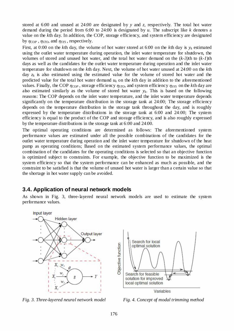
176

stored at 6:00 and unused at 24:00 are designated by y and z, respectively. The total hot water demand during the period from 6:00 to 24:00 is designated by u. The subscript like k denotes a value on the kth day. In addition, the COP, storage efficiency, and system efficiency are designated by COP , STO, and SYS , respectively. First, at 0:00 on the kth day, the volume of hot water stored at 6:00 on the kth day is yk estimated using the outlet water temperature during operation, the inlet water temperature for shutdown, the volumes of stored and unused hot water, and the total hot water demand on the (k-3)th to (k-1)th days as well as the candidates for the outlet water temperature during operation and the inlet water temperature for shutdown on the kth day. Next, the volume of hot water unused at 24:00 on the kth day zk is also estimated using the estimated value for the volume of stored hot water and the predicted value for the total hot water demand uk on the kth day in addition to the aforementioned values. Finally, the COP COP , storage efficiency STO, and system efficiency SYS on the kth day are also estimated similarly as the volume of stored hot water yk. This is based on the following reasons: The COP depends on the inlet water temperature, and the inlet water temperature depends significantly on the temperature distribution in the storage tank at 24:00; The storage efficiency depends on the temperature distribution in the storage tank throughout the day, and is roughly expressed by the temperature distributions in the storage tank at 6:00 and 24:00; The system efficiency is equal to the product of the COP and storage efficiency, and is also roughly expressed by the temperature distributions in the storage tank at 6:00 and 24:00. The optimal operating conditions are determined as follows: The aforementioned system performance values are estimated under all the possible combinations of the candidates for the outlet water temperature during operation and the inlet water temperature for shutdown of the heat pump as operating conditions; Based on the estimated system performance values, the optimal combination of the candidates for the operating conditions is selected so that an objective function is optimized subject to constraints. For example, the objective function to be maximized is the system efficiency so that the system performance can be enhanced as much as possible, and the constraint to be satisfied is that the volume of unused hot water is larger than a certain value so that the shortage in hot water supply can be avoided.

3.4. Application of neural network models As shown in Fig. 3, three-layered neural network models are used to estimate the system performance values.

Fig. 3. Three-layered neural network model Fig. 4. Concept of modal trimming method

177

As aforementioned, each system performance value is estimated independently by the corresponding model. For long-term operation of existing systems, it is necessary to measure necessary data continuously and identify model parameter values repeatedly, and estimate system performance values correspondingly. Here, the estimation only for short-term operation is considered. In the input layer, the operating conditions, the volumes of stored and unused hot water, and the total hot water demand on the past days as well as the operating conditions on the current day are adopted commonly as the inputs to the model to estimate all the system performance values. The estimated volume of stored hot water and the predicted total hot water demand on the current day are adopted additionally to estimate the volume of unused hot water. In the other layers, each neuron has multiple inputs and single output, and converts the weighted sum of the J inputs Xj minus the threshold to the output Y by the following response function:

Where j is the weight for each input. The sigmoid function is usually used as the response function g(x). In this paper, however, the hyperbolic tangent function g(x) = tanh x is used to obtain positive and negative values from the output. Here, the value from the output ranges only from -1.0 to 1.0 by normalizing the values to the inputs and from the output in advance.

3.5. Identification of model parameter values To estimate the system performance values by the neural network models, it is necessary to identify the values of model parameters, weights and thresholds in Eq. (1). The squared error between the estimated value and the corresponding measured value is evaluated for each pattern, and its summation for all the patterns is minimized as the objective function to identify the values of model parameters. In the back propagation method, the error function for each pattern is minimized sequentially. Here, to secure the local optimality of solutions and make the convergence faster, the total error function for all the patterns is minimized simultaneously. The search for local optimal solutions can be conducted by gradient methods for unconstrained nonlinear programming problems such as steepest descent, conjugate gradient, and quasi-Newton methods. However, these methods have the significant drawback that they can derive only local optimal solutions. In this paper, the modal trimming method proposed for nonlinear programming problems is adopted as a global optimization one [23]. This method has been applied to a neural network model for energy demand prediction, and its validity and effectiveness have been ascertained [24]. The concept of the modal trimming method is shown in Fig. 4. This method is composed of the following two procedures: A local optimal solution is searched to obtain a tentative global quasi-optimal one; A feasible solution with the value of the objective function equal to or smaller than that for the tentative global quasi-optimal one is searched to obtain an initial point for finding a better local optimal one. These procedures are repeated until a feasible solution with the value of the objective function equal to or smaller than that for the tentative global quasi-optimal one cannot be found, and the tentative global quasi-optimal one is adopted as the global quasi-optimal one. A local optimal solution is searched by a conventional gradient method. On the other hand, a feasible solution is searched by an extended Newton-Raphson method based on the Moore-Penrose generalized inverse of the Jacobi matrix of the objective function. The method can have a high possibility of deriving global optimal solutions, if it has the capability of global search for feasible ones. The renewal of the values of the variables based on the extended Newton-Raphson method has the following features: In the region with a feasible solution, the renewal can have the convergence to it; In the region with no feasible solution, the renewal can create a chaotic behavior and has the

178

capability of global search; In the region with no feasible solution, the renewal can also create a cyclically vibrating behavior and has the possibility of trap into a local optimal solution. To prevent the trap, a decelerating parameter is changed randomly in the range from 0.0 to 1.0 at each renewal.

4. Numerical study on performance estimation First, the parameter values of the neural network models are identified based on the system performance values obtained by numerical simulation, and their validity is investigated by comparing the estimated and simulated system performance values.

4.1. Numerical simulation It is necessary to use some system performance values to identify the values of model parameters. In applying the method of performance estimation to existing systems, measured data on system performance values must be used. In this paper, values obtained by numerical simulation are used in place of measured values. Here, only a summary on the numerical simulation is described as follows: A simplified static model is adopted for the CO2 heat pump [21]: Although the heat pump includes several components, they are not taken into account explicitly, and it is expressed by one model. The mass flow rates and temperatures of water at the inlet and outlet, COP, heat output, power consumption, and air temperature are adopted as basic variables whose values are to be determined. The mass and energy balance relationships as well as the energy input and output relationship are adopted as basic equations to be satisfied. The remaining equations to be considered are approximate functions of the power consumption and COP, and they are expressed in relation to the air and inlet/outlet water temperatures. A detailed dynamic model is adopted for the storage tank [19, 21]. To consider the one-dimensional vertical temperature distribution in the storage tank, it is vertically divided into many control volumes with the same volume, in each of which the water temperature is assumed to be constant. It is also assumed that the heat transfer occurs by water flow and heat conduction as well as heat loss from the tank surface. The mass flow rates and temperatures of water for each control volume are adopted as basic variables whose values are to be determined. The mass and energy balance relationships for each control volume are adopted as basic equations to be satisfied. A static model is adopted for the mixing valve. The mass flow rates and temperatures of water at the inlets and outlet are considered as basic variables, and the mass and energy balance relationships are considered as basic equations. At the connection points among the heat pump, storage tank, and mixing valve, connection conditions are taken into account to equalize the values of the corresponding variables. The outlet water temperature is given as a control condition. The feed water temperature as well as the mass flow rate and temperature of hot water to the tapping site are given as boundary conditions. The air temperature is given as an ambient condition. As for the concrete formulation of the simulation model, refer to reference [21]. The validity of the simulation model has been verified through an experiment and a three-dimensional thermo-fluid numerical simulation. As for this verification, also refer to reference [21]. The aforementioned modeling for the performance analysis by numerical simulation is conducted by a building block approach. The equations for the heat pump and mixing valve are static, while those for the storage tank are dynamic. Therefore, the modeling results in a set of nonlinear differential algebraic equations. It is solved by a hierarchical combination of the Runge-Kutta and Newton-Raphson methods.

179

Table 1. Specifications of CO2 heat pump water heating system

Equipment Specification Value CO2 heat

pump Rated heat

output 4.50 kW

Volume 370 L Height 1.45 m

Diameter 0.57 m Hot water storage tank Overall heat

transfer coefficient

0.80 W/(m2·°C)

Fig. 5. Performance characteristics of CO2 heat pump

4.2. Conditions for numerical simulation A numerical simulation is conducted to obtain the daily changes in system performance values under a daily change in a simulated hot water demand. The following are the conditions used in the numerical simulation: Table 1 shows the specifications of the CO2 heat pump water heating system. The values of model parameters included in the equations are estimated based on measured data for an existing system. The rated heat output of the heat pump is set at 4.5 kW. As an example, Fig. 5 shows measured values and approximate functions for the power consumption, COP, and their resultant heat output of the heat pump in relation to the inlet water temperature for the air and outlet water temperatures of 16 and 85 °C, respectively. Here, each value is relative to its rated one for the air and inlet/outlet water temperatures of 16, 17, and 65 °C, respectively. This is because the existing system used here was developed initially by a manufacturer, and the values of COP of existing systems have been enhanced significantly afterwards. The volume of the storage tank is set at 370 L. The number of control volumes for the storage tank is set at 200, and the sampling time interval for the Runge-Kutta method is set at 10 and 180 s for the cases with and without water flow, respectively. The mid-season is selected, and the corresponding air and feed water temperatures are set at 16 and 17 °C, respectively, which are prescribed by the Japanese Industrial Standards [25]. The numerical simulation is conducted for 6 representative days and a month, or consecutive 30 days composed of the 6 representative days [26]. On each representative day, an hourly change in a simulated hot water demand is prescribed. Figure 6 shows the total hot water demands on the 6 representative days. The 1st and 2nd representative days correspond to holidays with smaller and larger hot water demands, respectively, on which residents are out of the house. The 3rd and 4 th representative days correspond to weekdays with smaller and larger hot water demands, respectively. The 5th and 6th representative days correspond to holidays with smaller and larger hot water demands, respectively, on which residents are in the house. As an example, Fig. 7 shows the hourly change in the hot water demand on the 4th representative day. Here, the height and thickness of each vertical line means the flow rate and duration, respectively. The temperature of hot water supplied to the tapping site is set at 42 °C. Figure 8 shows the daily change in the total hot water demand on the 30 consecutive days.

180

Fig. 6. Total hot water demands on 6 Fig. 7. Hourly change in hot water demand representative days on 4th representative day

Fig. 8. Daily change in total hot water demand on consecutive 30 days

Table 2. Operating conditions for identification and verification of neural network models

The heat pump is started up at 0:00 and 1:00, when the total hot water demand on the previous day is larger than or equal to and smaller than 500 L/d, respectively. The outlet water temperature during operation is selected among 65, 75, and 85 °C, and the inlet water temperature for shutdown is selected among 30, 40, and 50 °C. The daily operating conditions are set by combining these values. 72 cases are investigated by the numerical simulation. Table 2 shows the conditions on the outlet water temperature during operation and the inlet water temperature for shutdown in cases 1 to 72. Cases 1 to 71 are used to identify model parameter values, while case 72 is used to verify the validity of model parameter values. In cases 1 to 54, the numerical simulation is conducted for the periodically steady state on each representative day under each combination of the constant outlet and inlet water temperatures. In cases 55 to 63, the numerical simulation is conducted on the consecutive days under each combination of the constant outlet and inlet water temperatures. In cases 64 to 66, the numerical simulation is conducted on the consecutive days under variable outlet water temperature and each constant inlet water temperature. In cases 67 to 69, the numerical simulation is conducted on the consecutive days under each constant outlet water temperature and

181

variable inlet water temperature. In cases 70 to 72, the numerical simulation is conducted on the consecutive days under variable outlet and inlet water temperatures. In cases 1 to 54, the initial temperature in the storage tank at 0:00 on the 1st day is set at 17 °C. In cases 55 to 72, the initial temperature distribution in the storage tank at 0:00 on the 1st day is set as follows: Since the 1st day corresponds to the 4th representative day as shown in Fig. 8, the temperature distribution in the storage tank at 0:00 obtained for the periodically steady state on the 4th representative day is adopted as the initial temperature distribution in the storage tank at 0:00 on the 1st day.

4.3. Conditions for performance estimation The numbers of neurons for the neural network models used for the performance estimation are set as follows: The data on the past two days are used; The numbers of neurons in the input and output layers are 12 and 1, respectively, for the models to estimate the COP, storage and system efficiencies, and volume of stored hot water; The numbers of neurons in the input and output layers are 14 and 1, respectively, for the model to estimate the volume of unused hot water; The number of neurons in the hidden layer is 3 commonly for all the models.

4.4. Results and discussion Figure 9 shows the operating conditions and the system performance values in case 70. Figure (a) shows the operating conditions given in advance, and Figs. (b) and (c) show the system efficiency, and the volumes of stored and unused hot water, respectively, estimated by the neural network models under the given operating conditions. These figures also show the corresponding values obtained by the numerical simulation. The system efficiency is shown as the ratio of the system efficiency to its value on the 1st day. The estimated system performance values coincide well with the simulated ones. This result shows that the values of model parameters are identified properly by the global optimization method, and that the system performance values are estimated with high accuracy. Figure 10 shows the operating conditions and the system performance values in case 72. Figures (a) to (c) show the same items as aforementioned. Although these simulated system performance values are not used to identify the values of model parameters, the estimated system performance values coincide well with the simulated ones. This result shows that the system performance values are estimated with high accuracy by the same neural network models even under different daily changes in the operating conditions.

5. Numerical study on optimal operation Next, the operating conditions are determined optimally based on the estimation by the neural network models whose parameter values are identified previously.

5.1. Conditions for optimal operation It is important to enhance the system efficiency and prevent the shortage in hot water supply. In this paper, therefore, the system efficiency is maximized subject to a lower limit for the volume of hot water unused at 24:00. The outlet water temperature during operation and the inlet water temperature for shutdown are adopted as the variables, and their values are determined so as to attain the objective and satisfy the constraint. Here, the lower and upper limits for the outlet water temperature during operation are set at 65.0 and 85.0 °C, respectively, and those for the inlet water temperature for shutdown are set at 30.0 and 50.0 °C, respectively.

182

On each day, each system performance value is estimated for all the combinations for the outlet and inlet water temperatures. For simplicity, the outlet water temperature is selected among its discrete values set by 1 °C from 65.0 to 85.0 °C, and the inlet water temperature is selected among its discrete values set by 1 °C from 30.0 to 50.0 °C. Here, the outlet water temperature is constrained so that the stratification in the storage tank is kept. Based on this estimation, the combination of the outlet and inlet water temperatures is selected so that the estimated system efficiency has its maximum and the estimated volume of unused hot water is larger than its lower limit.

Fig. 9. Daily changes in operating conditions Fig. 10. Daily changes in operating conditions and system performance values in case and system performance values in case

70: a) operating conditions, b) ratio of 72: a) operating conditions, b) ratio of system efficiency, c) volumes of stored system efficiency, c) volumes of stored

and unused hot water and unused hot water In case there is no combination by which the estimated volume of unused hot water is larger than its lower limit, the combination by which the estimated volume of unused hot water is the closest to its lower limit is selected.

183

In the numerical study, the lower limit for the volume of unused hot water is changed by 50 L from 50 to 250 L in cases 73 to 77, respectively, and its influence on the system performance is investigated.

Fig. 11. Daily changes in operating conditions Fig. 12. Daily changes in operating conditions

and system performance values in case and system performance values in case 73: a) operating conditions, b) ratio of 75: a) operating conditions, b) ratio of system efficiency, c) volumes of stored system efficiency, c) volumes of stored

and unused hot water. and unused hot water.

5.2. Results and discussion Figures 11 to 13 show the operating conditions and the system performance values in cases 73, 75, and 77, respectively. Figure (a) shows the operating conditions determined optimally, and Figs. (b) and (c) show the system efficiency, and the volumes of stored and unused hot water, respectively, estimated by the neural network models under the optimal operating conditions. These figures also show the corresponding values obtained by the numerical simulation. Although these operating

184

conditions and the corresponding system performance values are not used to identify the values of model parameters, the estimated system performance values coincide well with the simulated ones. This result shows that the system performance values are estimated with high accuracy by the same neural network models even under daily changes in the optimal operating conditions.

Fig. 14. Relationship between monthly system performance values

Fig. 15. Comparison between monthly system performance values under optimal and non-optimal operating conditions

Fig. 13. Daily changes in operating conditions and system performance values in case 77: a) operating conditions, b) ratio of system efficiency, c) volumes of stored and unused hot water

185

In case 75, as shown in Fig. 12, although the volume of unused hot water changes around 150 L, it becomes larger than 150 L on a few days. This is because both the operating conditions attain their lower limits, or the outlet water temperature attains the temperature at the top of the storage tank on those days. As a result, the daily change in the volume of unused hot water is small. In case 73, as shown in Fig. 11, the volume of unused hot water changes above 50 L on many days. This is also because both the operating conditions attain their lower limits, or the outlet water temperature attains the temperature at the top of the storage tank on those days. As a result, the daily change I the volume of unused hot water is large. On the other hand, in case 77, as shown in Fig. 13, the volume of unused hot water changes below 250 L on several days. This is because the operating conditions attain their upper limits on those days. As a result, the daily change in the volume of unused hot water is slightly large. Figure 14 shows the relationship between the lower limit for the volume of unused hot water and the monthly values of the ratio of system efficiency and the volume of unused hot water. The average value is adopted for the ratio of system efficiency, and the average, maximum, and minimum values are adopted for the volume of unused hot water. The average values of the ratio of system efficiency and the volume of unused hot water have a trade-off relationship. However, the average value of the ratio of system efficiency and the maximum or minimum value of the volume of unused hot water do not have a trade-off relationship. This is because, as shown in Figs. 11 and 13, in case the lower limit for the volume of unused hot water is small or large, the daily change in the volume of unused hot water becomes large, and the difference between the maximum and minimum values of the volume of unused hot water also becomes large. Figure 15 shows the comparison of the monthly values of the ratio of system efficiency and the volume of unused hot water in cases 70 to 77. The average value is adopted for the ratio of system efficiency, and the average and minimum values are adopted for the volume of unused hot water. As aforementioned, the average values of the ratio of system efficiency and the volume of unused hot water under the optimal operating conditions in cases 73 to 77 have a trade-off relationship. In addition, those under the non-optimal operating conditions in cases 70 to 72 are very close to the trade-off relationship. Thus, the optimal operation is not effective from the viewpoint of the average system performance values. On the other hand, the average value of the ratio of system efficiency and the minimum value of the volume of unused hot water under the optimal operating conditions in cases 73 to 77 have a trade-off relationship partly in cases 75 to 77. In addition, those under the non-optimal operating conditions in cases 70 to 72 are far from the trade-off relationship. As for the volume of unused hot water, the minimum value is more important than the average one to prevent the shortage in hot water supply. Thus, as shown by arrows, it is possible to enhance the average value of the system efficiency with the minimum value of the volume of unused hot water kept constant. The increases in the average value of the system efficiency are expected to be about 9.0, 9.9, and 8.2 % in cases 70 to 72, respectively.

6. Conclusions In this paper, a method of estimating the daily changes in system performance values by neural network models is proposed for a CO2 heat pump water heating system. In addition, the values of model parameters are identified by a global optimization method. Moreover, the operating conditions are determined optimally based on the system performance values obtained by the estimation. This approach is applied to estimating the daily changes in system performance values and determining the operating conditions optimally under a simulated monthly hot water demand, and its validity and effectiveness is investigated through the comparison between estimated and simulated system performance values. The following main results are obtained:

186

It is possible by this approach to estimate all the system performance values, or COP, storage and system efficiencies, and volumes of stored and unused hot water with high accuracy not only under the operating conditions used for identifying model parameter values but also under different operating conditions including the optimal ones.

It is important to enhance the system performance and prevent the shortage in hot water supply. It is possible by this approach to determine the operating conditions optimally so as to maximize the system efficiency subject to a lower limit for the volume of unused hot water for the purpose.

It is possible by this approach to enhance the average value of the system efficiency with the minimum value of the volume of unused hot water kept constant by changing the non-optimal operating conditions to the optimal ones. The increase in the average value of the system efficiency is expected to be 8 to 10 % under the conditions investigated in the numerical study.

Acknowledgment A part of this work was supported by the JSPS Grant- in-Aid for Scientific Research (C) No. 22560838.

References [1] Saikawa M. CO2 heat pump water heater. Energy and Resources 2004; 25 (2): 101–105 (in

Japanese). [2] Hashimoto K. Technology and market development of CO2 heat pump water heaters (ECO

CUTE) in Japan. IEA Heat Pump Centre Newsletter 2006; 24 (3): 12–16. [3] Hwang Y, Radermacher R. Theoretical evaluation of carbon dioxide refrigeration cycle.

International Journal of Heating, Ventilating, Air-Conditioning and Refrigerating Research 1998; 4 (3): 1–20.

[4] Nekså P, Rekstad H, Zakeri R, Schiefloe PA. CO2-heat pump water heater: characteristics, system design and experimental results. International Journal of Refrigeration 1998; 21 (3): 172–179.

[5] Saikawa M, Hashimoto K, Hasegawa H, Iwatsubo T. Study on efficiency and control method o f CO2 heat pump, report no. W98004. Central Research Institute of Electric Power Industry, 1999 (in Japanese).

[6] Saikawa M, Hashimoto K. Evaluation on efficiency of CO2 heat pump cycle for hot water supply-evaluation on theoretical efficiency and characteristics. Transactions of the JSRAE 2001; 18 (3): 217–223 (in Japanese).

[7] Nekså P. CO2 heat pump systems. International Journal of Refrigeration 2002; 25 (4): 421–427. [8] White SD, Yarrall MG, Cleland DJ, Hedley RA. Modelling the performance of a transcritica l

CO2 heat pump for high temperature heating. International Journal of Refrigeration 2002; 25 (4): 479–486.

[9] Skaugen G, Nekså P, Pettersen J. Simulation of trans-critical CO2 vapour compression systems. Proceedings of the 5th IIR-Gustav Lorentzen Conference on Natural Working Fluids, Guangzhou, 2002; 82–89.

[10] Richter MR, Song SM, Yin JM, Kim MH, Bullard CW, Hrnjak PS. Experimental results of transcritical CO2 heat pump for residential application. Energy 2003; 28 (10): 1005–1019.

[11] Yokoyama R, Shimizu T, Takemura K, Ito K. Performance analysis of a hot water supply system with a CO2 heat pump by numerical simulation (1st report, modeling and analysis o f heat pump). JSME International Journal, ser. B 2006; 49 (2): 541–548.

187

[12] Laipvadit P, Tiansuwan J, Kiatsiriroat T, Aye L. Theoretical performance analysis of heat pump water heaters using carbon dioxide as refrigerant. International Journal of Energy Research 2008; 32 (4): 356–366.

[13] Yan JL, Ma YT, Li MX, Hua J. Modeling and simulating the transcritical CO2 heat pump system. Energy 2010; 35 (12): 4812–4818.

[14] Sarkar J, Bhattacharyya S, Ram Gopal M. Performance of a transcritical CO2 heat pump for Simultaneous water cooling and heating. ASHRAE Transactions 2010; 116 (1): 534–541.

[15] Yamaguchi S, Kato D, Saito K, Kawai S. Development and validation of static simulation model for CO2 heat pump. International Journal of Heat and Mass Transfer 2011; 54 (9–10) : 1896–1906.

[16] Cecchinato L, Corradi M, Fornasieri E, Zamboni L. Carbon dioxide as refrigerant for tap water heat pumps: a comparison with the traditional solution. International Journal o f Refrigeration 2005; 28 (8): 1250–1258.

[17] Stene J. Residential CO2 heat pump system for combined space heating and hot water heating. International Journal of Refrigeration 2005; 28 (8): 1259–1265.

[18] Minetto S. Theoretical and experimental analysis of a CO2 heat pump for domestic hot water. International Journal of Refrigeration 2011; 34 (4): 742–751.

[19] Yokoyama R, Shimizu T, Ito K, Takemura K. Influence of ambient temperatures on performance of a CO2 heat pump water heating system. Energy 2007; 32 (4): 388–398.

[20] Yokoyama R, Okagaki S, Wakui T, Takemura K. Influence of operation temperatures on performance of a CO2 heat pump water heating system. Journal of Environment and Engineering 2008; 3 (1): 61–73.

[21] Yokoyama R, Wakui T, Kamakari J, Takemura K. Performance analysis of a CO2 heat pump water heating system under a daily change in a standardized demand. Energy 2010; 35 (2): 718–728.

[22] Yokoyama R, Kohno Y, Wakui T, Takemura K. Performance analysis of a CO2 heat pump water heating system under a daily change in a simulated demand. Transactions of the JSRAE 2010; 27 (4): 355–364.

[23] Yokoyama R, Ito K. Capability of global search and improvement in modal trimming method for global optimization. JSME International Journal, ser. C 2005; 48 (4): 730–737.

[24] Yokoyama R, Wakui T, Satake R. Prediction of energy demands using neural network with model identification by global optimization, Energy Conversion and Management 2009; 50 (2) : 319–327.

[25] Japanese Industrial Standards Committee. Residential heat pump water heaters, standard no. JIS C 9220: 2011. Japanese Standards Association, 2011 (in Japanese).

[26] Ukaji M, Sawachi T, Akimoto T, Hori Y, Kuwasawa Y, Mae M, Hosoi A. Study on low energy and resource saving technologies for autonomous housing (part 6, basic schedule for the verification of energy consumption in daily human activities). Procedings of the SHASE Annual Conference, Nagoya, 2004; 209–212 (in Japanese).



188

Performance of a common-rail Diesel engine fuelled with rapeseed and waste cooking oils

A. Corsinia, V. Giovannonib, S. Nardecchiac, F. Rispolid, F. Sciullie and P. Venturinif a Dipartimento di Ingegneria Meccanica e Aerospaziale, Sapienza Università di Roma, Rome, Italy,

[email protected] b AzzeroCO2 s.r.l., Rome, Italy, [email protected]

c Dipartimento di Ingegneria Meccanica e Aerospaziale, Sapienza Università di Roma, Rome, Italy, [email protected]

d Dipartimento di Ingegneria Meccanica e Aerospaziale, Sapienza Università di Roma, Rome, Italy, [email protected]

e Dipartimento di Ingegneria Meccanica e Aerospaziale, Sapienza Università di Roma, Rome, Italy, [email protected]

f Dipartimento di Ingegneria Meccanica e Aerospaziale, Sapienza Università di Roma, Rome, Italy, [email protected], CA.

Abstract: The EU energy strategy for 2020 forces scientists and industries to develop new generation of bio-fuels and increase the use of the ones available nowadays. Straight vegetable oils (SVO) and waste cooking oils (WCO) could represent an interesting alternative fuel for Diesel engines, representing a good solution in some niches sectors (i.e., public transportation, hybrid or marine propulsion, etc.). As a matter of fact the use of SVO as fuel do not requires large production plants as in the case of biodiesel, thus it can be used in a large number of countries without requiring new costs. On the other hand SVO has some shortcomings due to the different characteristics comparing with the gasoil fuel. Main differences are related to its smaller heating value, a different density, and a larger viscosity, and this may provoke some problems to the injection system and power loss in a Diesel engine. Aim of this work is to analyse the behaviour of a Diesel engine in automotive configuration when fuelled with SVO and WCO, to study the feasibility of use them in small public transport hybrid vehicles. To this aim a series of bench tests are performed; results are here presented. Tests are performed using a turbocharged, four stroke, four cylinders, water cooled, common-rail multijet Diesel engine operating on Diesel fuel, rape-seed oil (RO) and waste cooking oil (WCO) are presented. The influence of fuel used on engine power, spe-cific consumption, efficiency, and exhaust opacity, are compared with those obtained fuelling with Diesel fuel.

Keywords: Straight vegetable oil; waste cooking oil; common-rail Diesel engine; bio-fuels.

1. Background The limited reserves of fossil fuels, the continuously increasing oil cost, and the environment pollu-tion due to the combustion of fossil fuels are forcing the countries to revise their energy policies and put more and more attention to renewable energy sources. EU recently approved a new Directive aiming at changing its energy strategy. The Directive 2009/28/EC [1] fixes three main challenging objectives for 2020: to reduce the greenhouse gas (GHG) emissions by 20%; to reduce the final en-ergy consumption by 20% (improving energy efficiency); to provide 20% of European energy con-sumption using renewable. A particular attention is also put to the use of fuels in transport. Indeed, the same Directive stats that by 2020 at least 10% of the whole fuels used in transport must be re-newable. This new approach to energy forces scientists and industries to develop new generation of bio-fuels and efficiently increase the use of the ones already available. For Diesel engines the most suitable solution nowadays is the use of bio-diesel (BD), the bio-fuel derived by vegetable oils. It can be used alone or in blend with Diesel fuel (DF) and it is widely studied and tested ([2]-[6]). Al-though BD is a suitable substitution of DF, in the last years the interest in the use of SVO as fuel

189

has been increasing. This is due to the fact that BD requires large production plants, thus accord-ingly big economical efforts, and also consumes energy. Besides, the possibility of using vegetable oil directly as a fuel would widen the available alternative to DF, and would allow a lot of countries to use this alternative thus reducing their dependence on fossil fuels. At the moment the availability of vegetable oil, as well as of land to dedicate to oilseed crops, do not allow to look at the SVO as a global alternative to DF. However it can be used in blend with gasoil or also alone in some niche applications, such as public transport, hybrid and marine propulsion, electricity generation units, etc.. The situation may change with the use of oil from algae which seems to be very promising ([7]-[10]). Despite there are several advantages in using the SVO as a fuel, it also may provoke some eco-nomical and technical problems. Focusing the attention to the latter aspect, there are two main is-sues related to the use of SVO as fuel: the first one is its environmental implication (i.e., pollution and energy consumption during SVO production, transport, etc.), and the second is how a Diesel engine behaves when fuelled with SVO (i.e., power loss, efficiency, etc.). Environmental implication can be analysed using the Life Cycle Assessment (LCA) approach. In this kind of analysis all the factors influencing the life of a product are considered and evaluated to study the actual environmental impact of the product itself for a particular application. Here the Ital-ian situation is considered, but the analysis might be applied to every other country and application. Today in Italy several small electricity generation units (<1 MWel) operate using RO (or SVO in general), but due to the scarcity of RO on the Italian market, plant managers turn more often to Eastern Europe countries (i.e., Romania, Hungary, Poland, etc.) for vegetable oil supply. This has an environmental cost that may overcome the advantages due to the use of a bio-fuel. In a previous study [11] some of the authors evaluated the LCA of such a situation. It came out that, due to the fact that oilseed crops productivity in those countries (i.e., Romania) is not very high, part of the advantage of using RO as a fuel is loss during production and transport. Nevertheless, the GHG sav-ing (with reference to the use of DF) is still large, about 54% [11]. On the contrary, in the case of WCO collected through a short chain (maximum 70 km far from the power plant) the GHG emis-sions are extremely low. This is due to two main reasons: first, WCO is a waste product thus no emissions should be accounted for its production; second, the short chain reduces the emissions due to fuel transport. These aspects make the WCO an extremely interesting fuel from the GHG emis-sions point of view. Fig. 1 shows the GHG emissions caused by the use of RO and WCO as fuel in comparison with two conventional power production approaches, that is production using DF or electricity bought from the national grid. It is evident the advantage of using WCO or RO instead of the conventional solutions.

Fig. 1. GHGs emissions for four different Italian scenarios.

190

Once the environmental advantages given by the use of these bio-fuels are clear, then a more tech-nical aspect has to be studied, that is the behaviour of an engine operating with SVO. Aim of this work is to analyse the behaviour of a Diesel engine configured for automotive (public transport) applications, fuelled with RO and WCO. This will be the focus of the sections 2-4. Con-cluding remarks will close the paper.

2. Fuel characteristics Even though Rudolf Diesel developed what would become the Diesel engine using peanuts oil as a fuel, oil products took over, and the engines were developed and optimized for them. This results in a wide diffusion of internal combustion engines (because of the past large availability of oil) but a very narrow adaptability to other fuels. The use of SVO or WCO in a Diesel engine may provoke problems due to different fuel characteristics. Average physical characteristics of several vegetable oils are listed in Table 1 [12],[13]. These are only indicative characteristics since they may vary quite widely according to the ground properties, the kind of crops, the productions process, etc.. Generally speaking, SVO has lower calorific value with reference to DF (about 10-15% less), and an higher density. This reduces the difference in energy content when considering a fixed volume of fuel. Indeed, the volumetric heating value of SVO results only 5-6% less than that of DF. At room temperature SVO viscosity is about 10-30 times larger than that of DF, thus resulting in possible problems to the feeding and injection systems, and to the combustion chamber [12]-[17]. The cetane number of the reported SVO varies between 32 and 45 as opposed to 45-55 of DF. Since the cetane number is a measure of the flammability of a fuel it may result in combustion problems when the engine is cold. Flash point measures the temperature at which the vapours given off by a substance. SVO has a higher flash point as compared to DF, and this increases the safety of the former in the storage or in the transport phase.

Table 1. Average characteristics of some vegetable oils and DF ([12],[13]).

Oil Net heating

value (MJ/kg)

Density (kg/m3)

Kinematic viscosity (mm2/s)

Cetane number

Flash point (°C)

Diesel fuel 39.5-43.8 830-860 3.0-7.5 50 76-93 Palm 36.9 915-918 95.0-106.0 38-42 267-280

Rapeseed 37.4-39.7 911-915 77.0 32-38 246-320 Sunflower 37.1-37.7 916-925 55.0-61.0 35-37 274-316 Soybean 37.3-39.6 914-920 58.0-63.0 36-38 254-330 Jatropha 38.8 915 55.0 45 240

Table 2. Reference characteristics of RO, WCO and DF.

Oil Net heating

value (MJ/kg)

Density at 20°C (kg/m3)

Kinematic Viscosity at

20°C (Pa·s)

DF 43.3 [18] 868.88 6.33E-03 RO 37.6 [18] 960.85 51.54E-03

WCO 36.9 [14] 963.44 91.59E-03 In the present study RO and WCO will be used as fuel. Their characteristics are reported in Table 2 together with DF ones. Density and viscosity may remarkably vary with temperature, hence it is important to know their variation in order to exactly compute the engine performance and to avoid problem with the pump-

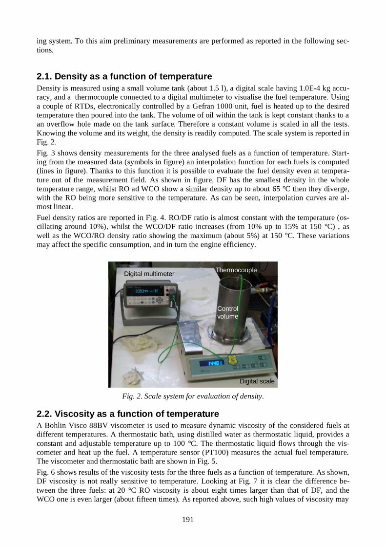
191

ing system. To this aim preliminary measurements are performed as reported in the following sec-tions.

2.1. Density as a function of temperature Density is measured using a small volume tank (about 1.5 l), a digital scale having 1.0E-4 kg accu-racy, and a thermocouple connected to a digital multimeter to visualise the fuel temperature. Using a couple of RTDs, electronically controlled by a Gefran 1000 unit, fuel is heated up to the desired temperature then poured into the tank. The volume of oil within the tank is kept constant thanks to a an overflow hole made on the tank surface. Therefore a constant volume is scaled in all the tests. Knowing the volume and its weight, the density is readily computed. The scale system is reported in Fig. 2. Fig. 3 shows density measurements for the three analysed fuels as a function of temperature. Start-ing from the measured data (symbols in figure) an interpolation function for each fuels is computed (lines in figure). Thanks to this function it is possible to evaluate the fuel density even at tempera-ture out of the measurement field. As shown in figure, DF has the smallest density in the whole temperature range, whilst RO ad WCO show a similar density up to about 65 °C then they diverge, with the RO being more sensitive to the temperature. As can be seen, interpolation curves are al-most linear. Fuel density ratios are reported in Fig. 4. RO/DF ratio is almost constant with the temperature (os-cillating around 10%), whilst the WCO/DF ratio increases (from 10% up to 15% at 150 °C) , as well as the WCO/RO density ratio showing the maximum (about 5%) at 150 °C. These variations may affect the specific consumption, and in turn the engine efficiency.

Fig. 2. Scale system for evaluation of density.

2.2. Viscosity as a function of temperature A Bohlin Visco 88BV viscometer is used to measure dynamic viscosity of the considered fuels at different temperatures. A thermostatic bath, using distilled water as thermostatic liquid, provides a constant and adjustable temperature up to 100 °C. The thermostatic liquid flows through the vis-cometer and heat up the fuel. A temperature sensor (PT100) measures the actual fuel temperature. The viscometer and thermostatic bath are shown in Fig. 5. Fig. 6 shows results of the viscosity tests for the three fuels as a function of temperature. As shown, DF viscosity is not really sensitive to temperature. Looking at Fig. 7 it is clear the difference be-tween the three fuels: at 20 °C RO viscosity is about eight times larger than that of DF, and the WCO one is even larger (about fifteen times). As reported above, such high values of viscosity may

Digital multimeter

Control volume

Digital scale

Thermocouple

192

provoke problems to the fuel filters, the feeding system, the injectors, as well as combustion prob-lems due to weak spray of fuel. The viscosity of any fuel can be computed following the Mac-Coull’s equation [19]:

log log logA B T C

where: is the kinematic viscosity (in cSt); A = 0.6-0.8 is a model constant; B and C are constants experimentally determined; T is the temperature in K. In the present work the Mac-Coull’s equation is used as interpolating function of the experimental data (constants are reported in Table 4). Inter-polation curves are reported in Fig. 6 with temperature ranging from 15 to 150 °C. From Fig. 6 and Fig. 7 it can be seen that above 90 °C RO and WCO viscosities are very close to that of DF, being less than the double of it. Thus in the engine tests, temperature of the vegetable oils is maintained at not less than 90 °C.

Table 3. Values of the constants of the Mac-Coull equation for the present study. Oil A B C DF 0.8 -3.068 7.478 RO 0.8 -3.759 9.510

WCO 0.8 -3.856 9.808

Fig. 3. Experimental end interpolated data for fuel density at different temperatures.

3. Experimental setup The use of SVO as a fuel in automotive applications is growing and there are several small compa-nies producing kits to switch from DF to SVO. Some of them propose their products also for com-mon-rail engine, but so far very few studies involving real automotive common-rail engines have been performed. Recently Labeckas and Slavinskas [16] reported on the experiments performed on a direct-injection off-road Diesel engine fuelled with RO, but it was a low speed, naturally aspired, not common-rail engine. Fontaras et al. [15] used a Renault Laguna 1.9 dCi passenger car for their tests, but it was fuelled with a RO-DF blend (10% of RO). So the real effect of using SVO on these kind of applications is still not fully known. In the following sections the experimental setup and test results on a Diesel engine fuelled with RO and WCO are presented and discussed.

193

Fig. 4. Density ratios between the analysed fuels.

Fig. 5. Viscometer and thermostatic bath.

Fig. 6. Experimental end interpolated data for fuel dynamic viscosity at different temperatures.

Viscometer

Thermostatic bath

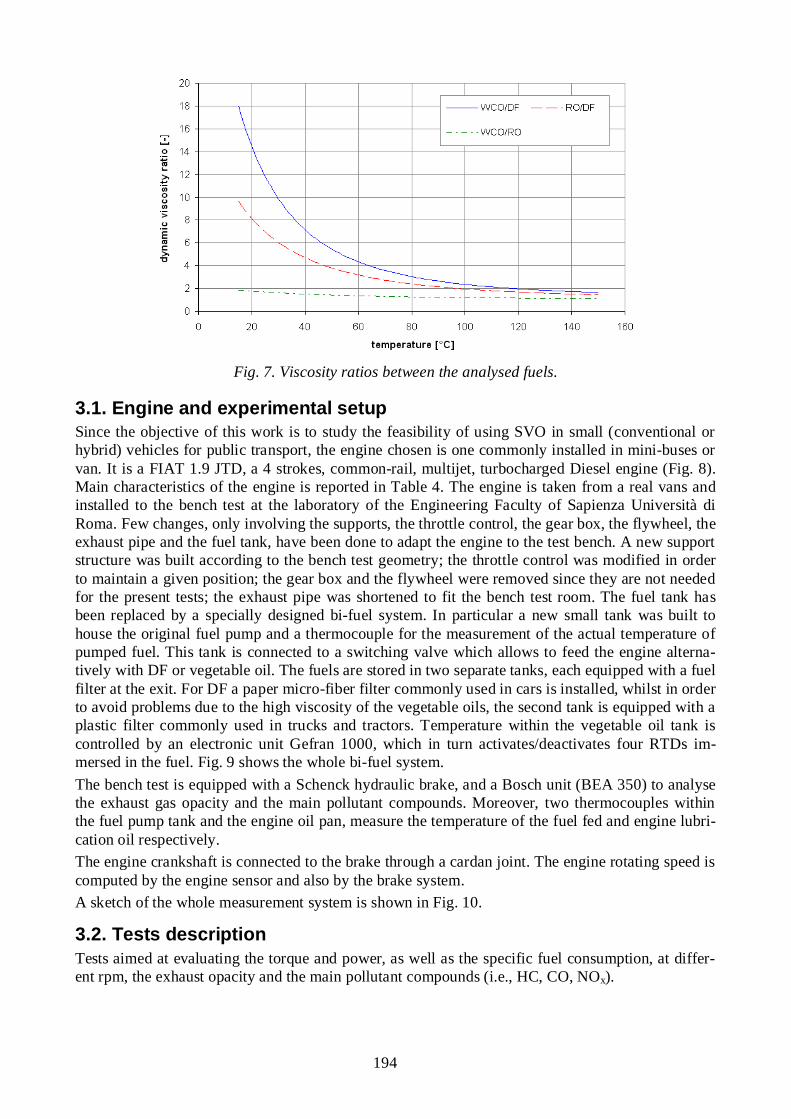
194

Fig. 7. Viscosity ratios between the analysed fuels.

3.1. Engine and experimental setup Since the objective of this work is to study the feasibility of using SVO in small (conventional or hybrid) vehicles for public transport, the engine chosen is one commonly installed in mini-buses or van. It is a FIAT 1.9 JTD, a 4 strokes, common-rail, multijet, turbocharged Diesel engine (Fig. 8). Main characteristics of the engine is reported in Table 4. The engine is taken from a real vans and installed to the bench test at the laboratory of the Engineering Faculty of Sapienza Università di Roma. Few changes, only involving the supports, the throttle control, the gear box, the flywheel, the exhaust pipe and the fuel tank, have been done to adapt the engine to the test bench. A new support structure was built according to the bench test geometry; the throttle control was modified in order to maintain a given position; the gear box and the flywheel were removed since they are not needed for the present tests; the exhaust pipe was shortened to fit the bench test room. The fuel tank has been replaced by a specially designed bi-fuel system. In particular a new small tank was built to house the original fuel pump and a thermocouple for the measurement of the actual temperature of pumped fuel. This tank is connected to a switching valve which allows to feed the engine alterna-tively with DF or vegetable oil. The fuels are stored in two separate tanks, each equipped with a fuel filter at the exit. For DF a paper micro-fiber filter commonly used in cars is installed, whilst in order to avoid problems due to the high viscosity of the vegetable oils, the second tank is equipped with a plastic filter commonly used in trucks and tractors. Temperature within the vegetable oil tank is controlled by an electronic unit Gefran 1000, which in turn activates/deactivates four RTDs im-mersed in the fuel. Fig. 9 shows the whole bi-fuel system. The bench test is equipped with a Schenck hydraulic brake, and a Bosch unit (BEA 350) to analyse the exhaust gas opacity and the main pollutant compounds. Moreover, two thermocouples within the fuel pump tank and the engine oil pan, measure the temperature of the fuel fed and engine lubri-cation oil respectively. The engine crankshaft is connected to the brake through a cardan joint. The engine rotating speed is computed by the engine sensor and also by the brake system. A sketch of the whole measurement system is shown in Fig. 10.

3.2. Tests description Tests aimed at evaluating the torque and power, as well as the specific fuel consumption, at differ-ent rpm, the exhaust opacity and the main pollutant compounds (i.e., HC, CO, NOx).

195

3.2.1. Torque and power For all the tests performed with vegetable oil, the start and stop phases (about 10 minute each) are performed fuelling with DF. At the start, as the lube oil reaches about 100 °C, the tank housing the feed pump is almost completely emptied using the fuel draining valve (Fig. 10), and then the feed-ing system is switched to vegetable oil. After few minute the residual DF in the tank is completely used by the engine, thus the test can start. The maximum throttle extent is divided into six parts. Torque and power are measured at each of the six possible positions, and at several engine rpm (namely 4200, 3700, 3200, 2700, 2200, 1700, 1500, and 1250 rpm).

Fig. 8. The FIAT 1.9 JTD Multijet engine used for the tests campaign.

Table 4. Main characteristics of the engine used for the tests. Type 1.9 MultiJet Charge Turbocharge (with intercooler) Fuel Diesel fuel Displacement 1910 cc Power 89.5 kW (120 hp) Maximum torque 200 Nm

Fig. 9. Bi-fuel system.

SVO tank

Switch valve

DF tank feed

pump

Fuel filters

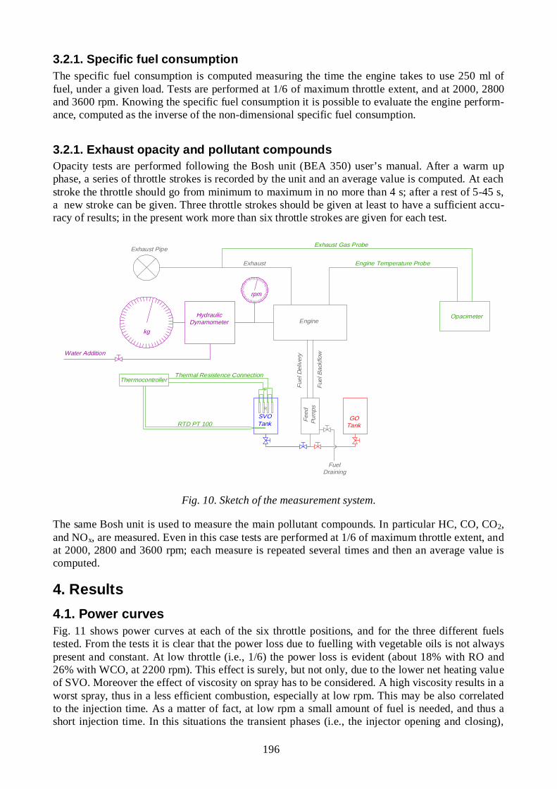
196

3.2.1. Specific fuel consumption The specific fuel consumption is computed measuring the time the engine takes to use 250 ml of fuel, under a given load. Tests are performed at 1/6 of maximum throttle extent, and at 2000, 2800 and 3600 rpm. Knowing the specific fuel consumption it is possible to evaluate the engine perform-ance, computed as the inverse of the non-dimensional specific fuel consumption.

3.2.1. Exhaust opacity and pollutant compounds Opacity tests are performed following the Bosh unit (BEA 350) user’s manual. After a warm up phase, a series of throttle strokes is recorded by the unit and an average value is computed. At each stroke the throttle should go from minimum to maximum in no more than 4 s; after a rest of 5-45 s, a new stroke can be given. Three throttle strokes should be given at least to have a sufficient accu-racy of results; in the present work more than six throttle strokes are given for each test.

HydraulicDynamometer Engine

Exhaust Pipe

kg

Opacimeter

Exhaust Gas Probe

SVOTank

GOTank

Feed

Pum

ps

Engine Temperature Probe

Thermocontroller

RTD PT 100

Thermal Resistence Connection

Fuel

Del

iver

y

Fuel

Bac

kflo

wWater Addition

FuelDraining

rpm

Exhaust

Fig. 10. Sketch of the measurement system.

The same Bosh unit is used to measure the main pollutant compounds. In particular HC, CO, CO2, and NOx, are measured. Even in this case tests are performed at 1/6 of maximum throttle extent, and at 2000, 2800 and 3600 rpm; each measure is repeated several times and then an average value is computed.

4. Results 4.1. Power curves Fig. 11 shows power curves at each of the six throttle positions, and for the three different fuels tested. From the tests it is clear that the power loss due to fuelling with vegetable oils is not always present and constant. At low throttle (i.e., 1/6) the power loss is evident (about 18% with RO and 26% with WCO, at 2200 rpm). This effect is surely, but not only, due to the lower net heating value of SVO. Moreover the effect of viscosity on spray has to be considered. A high viscosity results in a worst spray, thus in a less efficient combustion, especially at low rpm. This may be also correlated to the injection time. As a matter of fact, at low rpm a small amount of fuel is needed, and thus a short injection time. In this situations the transient phases (i.e., the injector opening and closing),

197

during which spray is not optimal, represent a relevant fraction of the whole injection time, thus combustion efficiency may be smaller than in the reference case. Power losses decrease as throttle increases, especially in the range around 2200-3200 rpm. Outside this range and with a throttle up to 3/6 power loss fuelling with RO and WCO is still remarkable. Curves with throttle at 4/6 show an inverse trend: there is a small range between 2200 and 3100 rpm where power loss fuelling with WCO is still clear, whilst fuelling with RO gives almost the same power as with the DF. Outside this range DF provides the smallest power, being the difference lar-ger at higher rpm. At 5/6 and 6/6 throttle, power curves are not really consistent: at 5/6 WCO pro-vides the highest power at any rpm, while RO stays below the DF curve up to about 3200 rpm then overcome it. On the contrary, at 6/6 throttle, power provided by vegetable oils returns to be smaller than that of DF, apart from two picks (at about 2000 rpm for RO, and 3300 rpm for WCO). This oscillating trends can be ascribed to the electronic unit control. It can check several parameters, such as the number of fuel jets, the fuel temperature, the exhaust temperature an composition, etc., and on the basis of their values the electronic unit tries to best fit the engine map recorded in it. Working with different fuels may then provoke an unpredictable behaviour of the electronic unit, hence engine operates irregularly.

Fig. 11. Power curves at different throttle positions for DF, RO and WCO: a) 1/6 throttle; b) 2/6 throttle; c) 3/6 throttle; d) 4/6 throttle; e) 5/6 throttle; f) full throttle.

a) b)

d) c)

e) f)

198

4.2. Specific fuel consumption and engine efficiency Fig. 12 shows the specific fuel consumption for DF, RO and WCO. In the range 2000-2800 rpm DF shows a specific consumption about 30% less than the two vegetable oils, which in that range show almost the same consumption. Above 2800 rpm fuel consumption increases as well as the differ-ence between DF and vegetable oils. Comparing the consumption at 3600 rpm it can be seen that the use of RO results in about 250% larger consumption with reference to DF case, whilst with WCO the difference approaches 300%. This larger specific consumption is the sum of three main effects: the lower net heating value and higher density of vegetable oils as compared to DF, and the electronic unit which, as written before, tries to match the map and the actual behaviour of the en-gine. Multiplying the specific fuel consumption by the net heating value of the fuels (Table 2) and invert-ing the quantity, the engine efficiency is computed. Fig. 13 shows about the engine efficiency evaluated on the basis of the specific fuel consumption tests. RO and WCO show the same effi-ciency. The difference with respect to the DF fuelling increases according to the rpm, starting from about 25% at 2000 rpm and approaching 50% at 3600 rpm.

Fig. 12. Specific fuel consumption curves.

Fig. 13. Engine efficiency.

199

4.3. Exhaust opacity The opacity of exhaust from DF is larger than those of WCO and RO (Fig. 14). This may be ex-plained considering the operative condition of the engine. Opacity of exhaust measures somehow particulate (soot) emissions produced during combustion. Soot is mainly formed in case of lack of oxygen and large presence of carbon. Comparing the formula of the DF and RO for instance (DF: C16H34, RO: C57H105O6, [18]) it is clear that vegetable oils have a larger content of carbon; neverthe-less they contain oxygen contrary to DF which does not contain it at all. Moreover the stoichiomet-ric air ratio is smaller for DF than for vegetable oils. Since the electronic unit regulates the air quan-tity ratio as if it is working with DF, when fuelling with vegetable oils it results in a higher air/fuel ratio, as confirmed by the lambda ratio measured by the Bosh unit (Fig. 15). This coupled with the larger content of oxygen, probably avoids the conditions for soot production when vegetable oils are used, even if their combustion is less efficient.

Fig. 14. Exhaust opacity.

Fig. 15. Lambda ratio.

4.4 Pollutant emissions Figs. 16-18 show the main pollutant compounds measured in the exhaust stream. CO emission is not shown because in all the tests it is null. Fig. 16 shows the HC concentration expressed as ppm. The three tested fuels show different behav-iours. In particular RO has the highest value of HC emission while WCO has the lowest one, both showing an almost linear behaviour with rpm (but different trend). The high HC emission level reached with RO can be related to its chemical composition. Indeed, vegetable oils have long C-chains which are broken during pre-combustion reactions. In WCO these long chains have been partially broken by the cooking process, thus it burns more easily and faster than RO. NOx emis-sions are shown in Fig. 17. RO and WCO produce lower NOx then DF. As reported in literature (i.e., [13]), this can be ascribed to the low heating value of RO and WCO. This reduces the peak

200

temperature within the cylinders and thus the thermal-NOx which give the main contribution to NOx emission in an internal combustion engine.

Fig. 16. HC emission. Fig. 17. NOx emission.

CO2 emitted by bio-fuels does not add to the greenhouse gas because it represents more or less the same quantity absorbed by plants during their growth. CO2 emissions for the three fuels used are shown in Fig. 18. In this case CO2 emission from DF is larger for each load in compare to those of RO and WCO, decreasing as rpm increases. As can be seen form the figure, at low rpm RO emis-sion is larger than that of WCO, inverting the trend as rpm increases.

Fig. 18. CO2 emission.

5. Conclusions Bench tests on a FIAT 1.9 JTD, a 4 strokes, common-rail, multijet, turbocharged Diesel engine, fu-elled with RO, WCO and DF are performed. The engine is in real automotive configuration, equipped with its original electronic unit. Beside bench tests, some preliminary tests are performed to determine the fuel density and viscosity as a function of temperature. Bench tests demonstrate that power loss due to the use of RO and WCO is relevant mainly at low loads (ranging from 18 to 26 %). At higher loads the power loss decreases and in some cases, vegetable oils provide a higher power as compared to DF. This behaviour may be due to several effects, i.e., the different density and viscosity of vegetable oils, the electronic unit, and the injection time which varies according to load. The use of RO and WCO results also in a different specific fuel consumption. This is clearly due to the lower net calorific value of vegetable oils, which is just partly reduced by their higher density.

201

This reflects on the engine efficiency which is smaller than that of DF, showing a difference which varies for 25% at low load, up to 50% at higher load. A positive result is obtained as for the exhaust opacity, since vegetable oils produce smaller values as compared to DF. This could be explained considering the chemical composition of vegetable oils. Soot forms mainly when a rich carbon fuel is used and in lack of oxygen. Since the oxygen is a main component of the vegetable oils, probably this avoid the conditions to let the soot form. Pol-lutant emissions are comparable to or less than those of DF, apart from HC emission from RO which reaches the highest level. This effect is probably related to the long C-chain compounds forming the RO. Despite the engine used for this work may operates with vegetable oils, the electronic unit and fuel characteristics play an important role in engine performance. Fuel characteristics (i.e., viscosity) may be controlled by pre-heating the fuel as demonstrated by the preliminary tests performed. Elec-tronic unit has to be tuned to work with vegetable oils, and this would be the next step of this re-search project.

Acknowledgments We thank the CURSA (University Consortium for Socio-economic and Environmental Research) Italy, especially Eng. S. Binotti and Eng. M. Napoleoni, for their interest and help in this project. We also thank Dr. L. Monteleone for the assistance given during tests; S. Nardecchia for its work and help in assembling and preparing the engine; and I. Campolo for the work done during tests.

References [1] Directive 2009/28/EC of the European Parliament and of the Council of 23 April 2009 on the

promotion of the use of energy from renewable sources and amending and subsequently repeal-ing Directives 2001/77/EC and 2003/30/EC. Available at: eur-lex.europa.eu.

[2] Canacki M., Combustion characteristics of a turbocharged DI compression ignition engine fu-eled with petroleum diesel fuels and biodiesel. Bioresource Technology 2007;98(6):1167-1175.

[3] Kalligeros S., Zannikos F., Stournas S., Lois E., Anastopoulos G., Teas Ch, Sakellaropoulos F., An investigation of using biodiesel/marine diesel blends on the performance of a stationary die-sel engine. Biomass and Bioenergy 2003;24(2):141-149.

[4] Wang G.W., Lyons D.W., Clark N.N., Gautam M., Norton P.M., Emissions from nine heavy trucks fuelled by diesel and biodiesel blend without engine modification. Environmental Scien-ce & Technology 2000;34(6):933-939.

[5] Lapuerta M., Armas O., Rodriguèz-Fernàndez J., Effect of biodiesel fuels on diesel engine emissions. Progress in Energy and Combustion and Science 2008;34(2):198:223.

[6] Ramadhas A.S., Muraleedharan C., Jayaraj S., Performance and emission evaluation of a diesel engine fuelled with methyl esters of rubber seed oil. Renewable Energy 2005;30(12):1789-1800.

[7] Vijayaraghavan K., Hemanathan K., Biodiesel production from freshwater algae. Energy & Fu-els 2009;23:5448-5453.

[8] Demirbas A., Fatih Demirbas M., Importance of algae oil as a source of biodiesel. Energy Con-version and Management 2011;52:163-170.

[9] Scott S.A., Davey M.P., Dennis J.S., Horst I., Howe C.J., Lea-Smith D., Smith A.G., Biodiesel from algae: challenges and prospects. Current Option in Biotechnology 2010;21:277-286.

[10] Demirbras A., Biodiesel from algae, biofixation of carbon dioxide by microalgae: a solution to pollution problems. Applied Energy 2011;88:3541-3547.

202

[11] Scarascia Mugnozza G., Binotti S., Napoleoni M., Rispoli F., Sciulli F., Venturini P., Bab-bini S., Straight vegetable oil as a fuel in an internal combustion engines for power and heat production. 4th Energy Conference – Palestine, 26-27 January, Ramallah, Palestine.

[12] Misra R.D., Murthy M.S., Straight vegetable oil usage in a compression ignition engine – A review. Renewable and Sustainable Energy Reviews 2010;14:3005-3013.

[13] Sidibé S.S., Blin J., Vaitilingom G., Azoumah Y., Use of crude filtered vegetable oil as a fuel in Diesel engines state of the art: literature review. Renewable and Sustainable Energy Re-views 2010;14:2748-2759.

[14] Pugazhvadivu M., Jeyachandran K., Investigation on the performance and exhaust emissions of a Diesel engine using preheated waste frying oil as fuel. Renewable Energy 2005;30:2189-2202.

[15] Fontaras G., Kousoulidou M., Karavalakis G., Bakeas E., Samaras Z., Impact of straight vegetable oil-diesel blends application on vehicle regulated and non-regulated emissions over legislated and real world driving cycles. Biomass and Bioenergy 2011;35:3188-3198.

[16] Labeckas G., Slavinskas S., Performance of direct-injection off-road diesel engine on rape-seed oil. Renewable Energy 2006;31:849-863.

[17] Hossain A.K., Davies P.A., Plant oils as fuels for compression ignition engines: A technical review and life-cycle analysis. Renewable Energy 2010;35:1-13.

[18] Altin R., Cetinkaya S., Husein S.Y., The potential of using vegetable oil fuels as fuel for diesel engine. Energy Conversion and Menagement 2001;42:529-538.

[19] Briant J., Denis J., Parc G., Propièteè rhèologiques des lubrifiants. Paris, France: Editions Technip et Institut Francais du Petrole; 1985.



203

Reduced Energy Cost through the Furnace Pressure Control in Power Plants

Vojislav Ž. Filipovi a, Novak N. Nedi b and Saša Lj. Prodanovi c

a University of Kragujevac, Faculty of Mechanical Engineering Kraljevo, Kraljevo, Serbia, [email protected] ,

b University of Kragujevac, Faculty of Mechanical Engineering Kraljevo, Kraljevo, Serbia, [email protected] ,

c University of East Sarajevo, Faculty of Mechanical Engineering, East Sarajevo, Bosnia and Herzego-vina, [email protected], CA

Abstract: Maintaining pressure in the boiler’s furnace is one of the key requirements for proper combustion in steam boilers in thermal power plants. This paper proposes a control strategy that eliminates flap in the channel for the output gases. This is achieved by applying the frequency regulator for asynchronous motor speed con-trol. Reference value for the frequency regulator is obtained through the PI controller. Special attention is given to tuning of PI controller. Well-tuned PI controller with the use of frequency regulator provides signifi-cant energy savings, because asynchronous motor for ventilator of steam boiler in thermal power plants has a large power. Modification of relay feedback experiment has supported -tuning of controller whose two types (faster and robust) were tuned. This modification consists in:

a) Replacement of relay characteristic with saturation curve,

b) Fourth-order process identification with first-order process plus dead time.

The methodology is illustrated by simulations.

Keywords: Energy saving, Combustion, Frequency regulator, PI controller, -tuning.

1. Introduction Steam boiler, as well as the other components of power plant, performs energy transformation. Therefore, energy dissipation, during combustion process, is present here. This paper considers and suggests possibilities for energy saving by changing in strategy of furnace pressure control as part of boiler. That means replacing of damping control with strategy which is based on frequency regulators (variable-speed drives). Namely, furnace output gases are controlled by ventilators (fans) instead by flap (valve) in output channel. The aim of this paper is to build new control loop for fur-nace pressure using frequency regulators for asynchronous motor speed control, which drives ven-tilator. In this control system, PI (proportional – integral) controller generates reference values for fre-quency regulator [1]. In order to explore an adequate tuning of PI controller, the method for process identification using relay feedback test was carried out using simulation. Saturation relay will be applied instead ideal relay because of its well known advantages [1]. Unlike previous research, fourth-order process was identified as true first-order process plus relative small dead time [2]. Af-terward, method of -tuning gives parameters of PI controller, which is adequate for first-order process. Because of the possibility of different conditions during operation of the system, two types of PI controller (faster and robust) will be tuned [1]. Their quality will be explored after simulation of entire control loop for furnace pressure and analysing of process response. Essentially, this sur-vey tends to exploit simulation as a tool for considering improvements of existing control system. Accordingly, researches in this paper are focused on reducing the energy consumption that is neces-

204

sary for the operation of thermal power plant, which directly means increasing the amount of elec-tricity for delivery to customers [3].

2. Model of system Good combustion in furnace of steam boiler enables better parameters of steam and better utiliza-tion of coal and in that way greater efficiency and lower costs. It is being obtained by maintenance of the furnace pressure on reference value which is required for well combustion. Furnace pressure control is necessary for controlling of quantities of O2 and CO during combustion process [4]. Mentioned pressure depends on air circulation through the furnace. There are four ventilators, one couple for input of air and the other for output of gases. Because of larger flow on outlet, furnace is under vacuum. It is shared in two parts: upper and lower. In following exposures two approaches of furnace pressure control will be presented.

2.1. Damping model for furnace pressure control This model is very widespread in thermal power plants. It is based on valve (flap) for furnace output gases. Therefore, asynchronous motors for ventilators always work with full power during exploita-tion. That causes energy dissipation on valves, as its main drawback, because output flow of gases is being controlled only by flap rotating. Namely, valves perform a damping here. Knowledge of the constituent components of the control system and connection between them and than their behav-iour equations have enabled the formation of a general block diagram of the said control system. Of course, as so often in the modelling, to simplify a constructed mathematical model assumptions have been introduced [5]. General block diagram for this strategy is shown in Fig. 1.

Fig. 1. General block diagram for damping control strategy [5]

2.2. Suggested model with frequency regulators High power of asynchronous motors for ventilators leads to significant possibilities for energy sav-ing by reducing their consumption. That might be enabled using frequency regulators for speed control of asynchronous motor. For example, in the thermal power plant Gacko (Bosnia and Herze-govina) both electric motors for ventilators in output channel of furnace have the same power P = 3,2 MW [6]. Configuration for application of this energy saving strategy is shown in Fig. 2, where dynamics of frequency regulators and pressure sensor haven’t been considered because of small values of their gains and time constants. Hence those transfer functions have been assumed as 1.

205

Fig. 2. General block diagram for strategy which is based on frequency regulators

In the both of strategies, gain and time constant of each component (i.e. transfer function) can be determined according physical laws or experimentally by recording their input and output signal. The meanings of indexes of those components (blocks) have been given in nomenclature. PI controller forms reference value for frequency regulator which is necessary for appropriate motor speed obtaining. Motor speed is being controlled by changing of power frequency. In order to keep constant torque, supply voltage should be controllable by frequency. In this way, frequency regula-tors provide power supply, which load (in our case ventilators) requires, and that is the key for en-ergy saving [7]. Namely, torque for fan (ventilator) is:

tktM f2

1 (1) power that should be obtained from the motor is:

tktPf3

2 (2)

where: t – angular speed, k1 and k2 – constants.

Now, reduction average speed of motor by 10% (which is usually feasible) leads to decrease in energy consumption by 27%, because it is calculated: 1 – (0,9)3 1 – 0,73 = 0,27. This approach involves omission of valves, electric motors for its drive, and other components such as gearboxes and valve position sensors and thus increases savings. In order to present general values of savings, here are calculated and shown in Table 1 possible sav-ings in mentioned thermal power plant Gacko, i.e. in its electric motors for ventilators. In this cal-culation was taken into account that that thermal power plant operates up to 7000 hours per year, because of its regular maintenance and unexpected failures.

Table 1. Energy saving of electric motor with reduction of its average speed by 10% Daily Annual

Consumption MWh

Energy saving MWh

Consumption MWh

Energy saving MWh

Electric motor for ventilator P=3,2x2=6,4 MW 153,6 41,5 44800 12096

Therefore, annual saving in the amount of 12,096 GWh is very significant and enables greater de-livery of electricity to consumers. In addition to energy saving frequency regulators allows: optimization of the process, “softer” functioning of driving and operating machines because of their smaller number of starts and stops, lower maintenance costs, longer equipment life and improved operating environment (for example, less fan noise). This theoretic approach, through these two control strategy, has been served as guideline for order assessment of process transfer function, which will be explained in next chapter.

206

3. Process identification The knowledge transfer function of the process opens the opportunities of its analysis but also tun-ing of PI controller by various methods. It can be found on two ways: by modelling based on physi-cal rules and using methodologies of identification. Relay feedback test, which is often used for autotuning of PI controllers, here has been utilized for process identification [2]. In real conditions, this procedure involves introducing relay (as nonlin-earity) into system in order to cause steady oscillations in its response and then obtain necessary in-formation of the process. That method will be simulated in Matlab software. For that purpose transfer function of process will be assumed. According general block diagram of system for furnace pressure control in Fig. 2, (where are four first-order components) this process can be taken as fourth-order process. Following exposure contains simulated and suggested meth-odology for process identification which is presented on example. Namely, in the absence of a real process model, transfer function is taken arbitrarily, as shown in Figs 4. and 7. In this case it is not disadvantage, but proof that the identification procedure which is carried out can be applied to any process. Relay feedback test is based on saturation relay because of its advantages over ideal relay in esti-mating of ultimate gain and ultimate period. In order to carry out process identification, i.e. obtain transfer function; following parameters should be determined [1]: K – steady state gain, L – dead time, T – time constant.

Then, this transfer function of first-order process is:

LseTs

KsG1

(3)

where: K= y/ u as it shown in Fig. 3.

Fig. 3. Process input and output

207

Order of transfer function is obtained depending on category of system (based on integrated absolute error from frequency response), which is determined by L/T ratio and assumed order of the process. According partially demonstration in [2], in this example process will be presented with first-order process plus relative small dead time, as it shown in (3). In the following chapter its validation will be proved. Now, mentioned parameters are given by [2] and follows: first iteration to compute time constant, hence

u

uLtgT1 (4)

afterwards, the second iteration follows

12ln2/

1/TLu

eTT (5)

and

1/1 TLehaK (6)

As previously stated, general procedure for identification will be presented on arbitrarily chosen process in folowing three steps: First step Performing relay feedback test using ideal relay to determine slope of saturation relay (k). Fig. 4. shows configuration for carry out relay feedback test in Matlab software.

Fig. 4. Configuration for ideal relay feedback test [8]

At the beginning, height of ideal relay characteristic h = 0,03 bar has been set as Fig. 5 shows. Be-cause h = 0,1·SP, where SP is set point of furnace pressure (in thermal power plant Gacko SP = 0,3 bar) [6]. This simulation gives relay output and relay feedback response, which is shown in Fig. 5 and 6, respectively.

Fig. 5. Ideal relay output

Ti me (s)

Am

plitu

de (b

ar)

208

(a) (b)

Fig. 6. Ideal relay feedback response: a) whole view, b) zoomed segment

Using diagrams in Fig. 6 amplitude of response has been determined: a = 0,0085 bar. Now, ultimate gain is [1]:

5,4a/4hK u (7)

where min

kK u ,

the slope of saturation relay is given by 3,64,1

minkk (8)

Second step Carry out relay feedback test using saturation relay as it is presented in Fig. 7., and result is diagram shown in Fig. 8.

Fig. 7. Configuration for saturation relay feedback test

(a) (b)

Fig. 8. Saturation relay feedback response: a) whole view, b) zoomed segment

209

Amplitude of response a = 0,0094 bar, dead time L = 2,21 s and ultimate period Tu = 2,82 s have been determined from diagrams in Fig. 8. Than ultimate frequency can be calculated:

71,0/2 uu T (9)

Third step Calculate necessary parameters to complete desired transfer function. Afterward, using (4), (5) and (6) required parameters are obtained: T1 = 2 s, T = 0,87 s and K = 0,47. Using (3) gives transfer function of process

ses

sG 21,2

187,047,0

It is very important to say that this process is described as true first-order process plus relative small dead time, because relay feedback response doesn’t develop stationary oscillation in the first cycle (Fig. 8), unlike the previous practice whereby this process should be described by high-order proc-ess without dead time, because ratio L/T = 2,54 [2].

4. Tuning of PI controller Since the process has been identified as first-order process, the best type of controller is PI. -tuning method (Dalin) will be used for obtaining appropriate parameters of controller. This

method is special case of method of pole design [1]. It is based on two assumptions: 1. integral time constant Ti is equal to time constant of the process T, 2. it is assumed that system’s feedback contains one real pole s = –1 / where is desired time

constant of that system. Approximation of exponential article in (3) with two article of Taylor progression gives

11

TsLsKsG (10)

Using first assumption transfer function of PI controller is

TsKsG cc

11 (11)

Than characteristic equation of system derived with (10) and (11) is 01 sGsG c (12)

Based on mentioned assumptions and (10), (11) and (12) parameters of PI controller are obtained as follows

LT

KKc

1 (13)

TTi (14)

According this method, heuristic rules are being used for determining of : = T for faster controller, = 3T for robust controller.

Afterward, parameters of PI controller for considered process are calculated: Kc = 0,6 and Ti = 0,69 for faster controller,

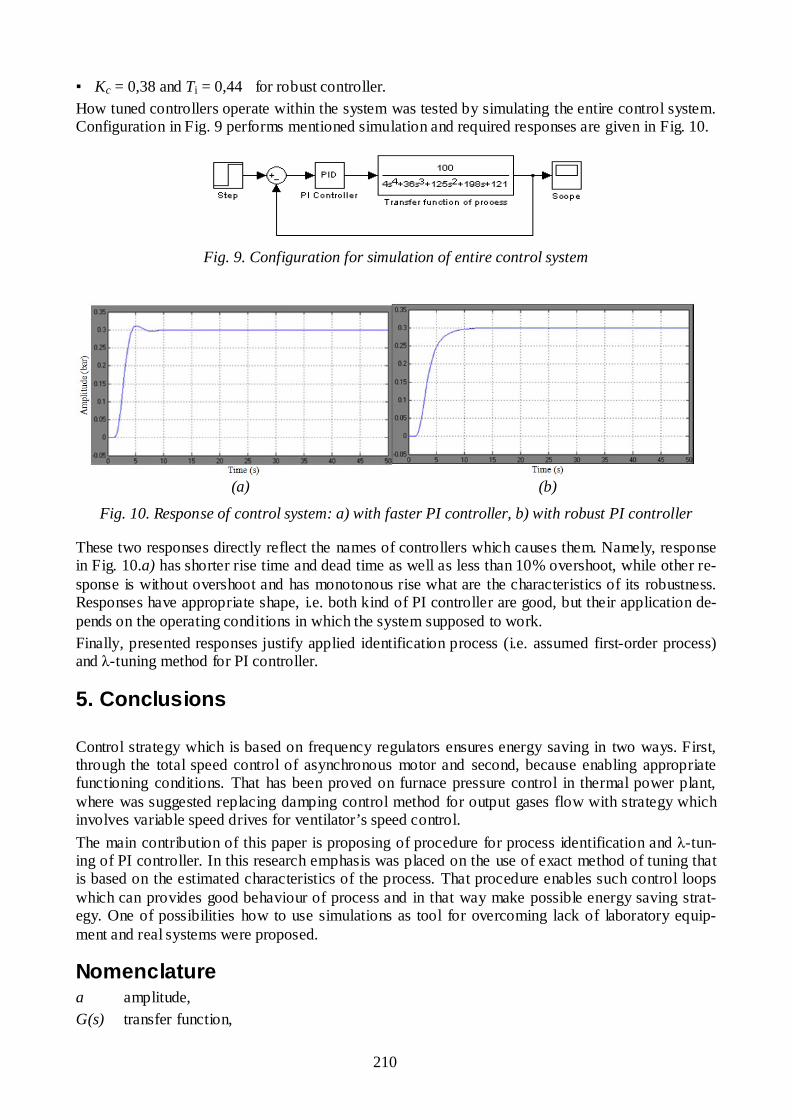
210

Kc = 0,38 and Ti = 0,44 for robust controller. How tuned controllers operate within the system was tested by simulating the entire control system. Configuration in Fig. 9 performs mentioned simulation and required responses are given in Fig. 10.

Fig. 9. Configuration for simulation of entire control system

(a) (b)

Fig. 10. Response of control system: a) with faster PI controller, b) with robust PI controller

These two responses directly reflect the names of controllers which causes them. Namely, response in Fig. 10.a) has shorter rise time and dead time as well as less than 10% overshoot, while other re-sponse is without overshoot and has monotonous rise what are the characteristics of its robustness. Responses have appropriate shape, i.e. both kind of PI controller are good, but their application de-pends on the operating conditions in which the system supposed to work. Finally, presented responses justify applied identification process (i.e. assumed first-order process) and -tuning method for PI controller.

5. Conclusions Control strategy which is based on frequency regulators ensures energy saving in two ways. First, through the total speed control of asynchronous motor and second, because enabling appropriate functioning conditions. That has been proved on furnace pressure control in thermal power plant, where was suggested replacing damping control method for output gases flow with strategy which involves variable speed drives for ventilator’s speed control. The main contribution of this paper is proposing of procedure for process identification and -tun-ing of PI controller. In this research emphasis was placed on the use of exact method of tuning that is based on the estimated characteristics of the process. That procedure enables such control loops which can provides good behaviour of process and in that way make possible energy saving strat-egy. One of possibilities how to use simulations as tool for overcoming lack of laboratory equip-ment and real systems were proposed.

Nomenclature a amplitude, G(s) transfer function,

211

h height of ideal relay characteristic, K steady state gain, k slope of saturation relay, L dead time, s P power, W s complex variable, T time constant, h t time, s U voltage, V Greek symbols

change of signal, desired time constant, s angular speed, s-1

Subscripts and superscripts c controller, em electric motor, f fan (ventilator), fl lower part of furnace, fu upper part of furnace, i integral, u input and ultimate, v valve, y output.

References [1] Filipovi VŽ, Nedi NN. PID Controllers. Kraljevo: University of Kragujevac, Faculty o f

Mechanical Engineering; 2008. (in Serbian). [2] Yu, CC. Autotuning of PID controllers. Taipei, Taiwan: National Taiwan University, Springer;

2006. [3] Prodanovi S. Analysis and improvement of control system of condensate level in condenser o f

turbine in thermal power plant Gacko (master thesis). Kraljevo, Serbia: University of Kragu-jevac; 2009. (in Serbian).

[4] Buljubaši I. Modelling of processes in steam boilers as a part of performance monitoring. TTEM Journal 2006;1(2):34 – 39.

[5] Komatsu T. Instrumentation for boiler plant. Fuji Denki Review;9(6):164 – 168. [6] Technical documentation of the control system of condensate level in condenser of turbine and

of the entire thermal power plant Gacko. [7] Filipovi V, Nedi N, Prši D, Dubonji LJ. Energy saving with variable speed drives. Proceed-

ings of the VI International Triennial Conference, Heavy Machinery – HM 2008: Kraljevo, Mataruška banja, pp. A1 – A6 .

[8] Prodanovi SLJ, Nedi NN, Filipovi VŽ. Improved Auto-tuning PID Controller of Level in Condenser of Turbine in Thermal Power Plant Using Saturation-relay Feedback. Proceedings o f the X Triennial International SAUM Conference on Systems, Automatic Control and Measurement, Niš, Serbia, 2010.



212

Short-term scheduling model for a wind-hydro-thermal electricity system

Sergio Pereira a, Paula Ferreira a A. Ismael F. Vaz a aDepartment of Production and Systems, University of Minho, Guimarães, Portugal

Abstract:

This study addresses the problem of the self-scheduling of an electricity system mainly based on hydro, fossil fuel thermal and wind power plants. A binary mixed integer non-linear optimization model is described and applied to short-term electricity planning of a system close to the expected Portuguese one on the year 2020. The model is written in a GAMS code and a global optimization solver is used to obtain the numerical results. The objective function encompasses the minimization of total system production costs through a centralized unit commitment. Different constraints, essentially related to operating parameters that characterize the power plants available for dispatch, are included in the model. The obtained results show the importance of the renewable energy sources seasonality on the thermal power plants operating conditions and on the total cost of the system.

Keywords: Electricity planning, Electricity system analysis, Unit Commitment problem.

1. Introduction The emergence of new technologies such as wind power, characterized by production of variable output, not subject to dispatch and benefiting from feed–in tariffs, creates new challenges to the electricity power management. On the contrary, the large thermal and hydropower groups need to compete in the market for dispatch. Also, adding more variability and unpredictability to a power system, due to wind power curve characteristics, will frequently originate that thermal units will experience increased number of startups and shutdowns, and periods of operation at low load levels (see [1]). It is well known that the principal aim of power planning, whether it is applied to long term planning horizon or to short term horizon, is to minimize the operational costs of the system while that a certain forecasted demand is fulfilled. In order to accomplish this aim, optimization models for both short-term electrical power generation scheduling and strategic power planning are seen as useful and powerful tools to be used by decision makers. Short-term electricity power generation scheduling, also known as unit commitment (UC) problem, is essential for the planning and operation of power systems. The basic goal of the UC problem is to properly schedule the on/off states of all the units in the system. Furthermore, the UC problem should consider the predicted load demand and spinning reserve requirement, minimizing the total cost of production [2]. Uyar, A. et al. in [3] described the short-term electrical power generation scheduling as an optimization problem, in which optimal startup and shutdown schedules, for a group of power generators, need to be determined over a given time horizon and considering operational constraints. The model objective remains as the minimization of the power generation costs meeting the hourly forecasted power demands. The short-term electricity power generation scheduling is well documented in the literature, with special concerns about the wind power penetration on the traditional thermal units systems, and on the market prices (see, for example, [4] and [1]). Despite the economic interests considered in these models, environmental concerns are also increasingly relevant. The Catalão, J. et al. study [5] focused on a multi-objective formulation, where two objective functions were considered, namely the total fuel cost and total CO2 emissions.

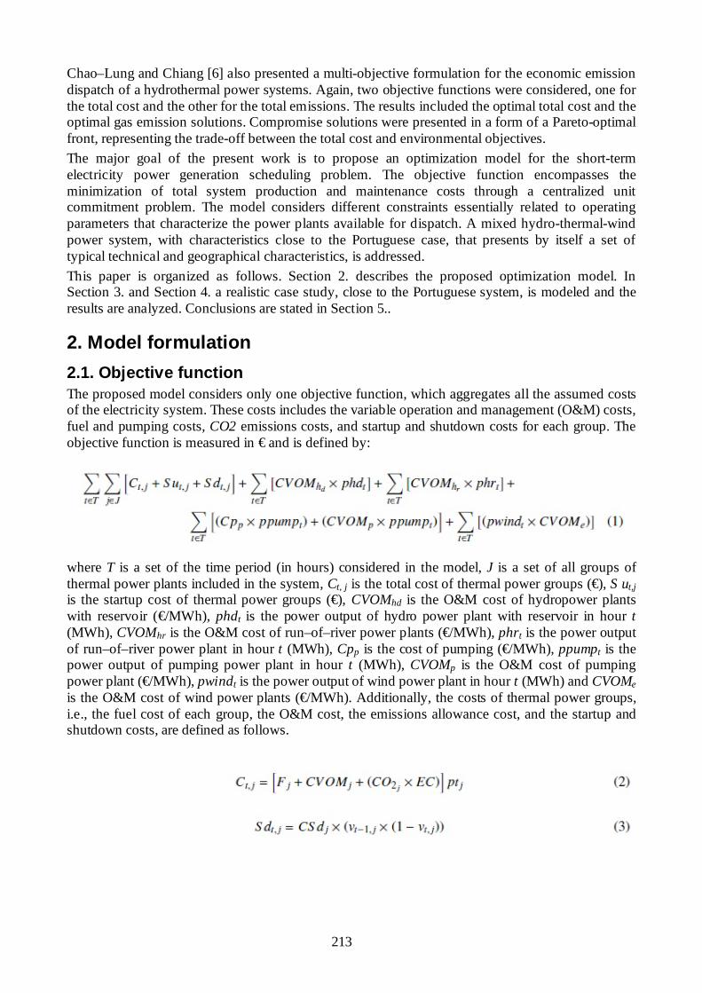
213

Chao–Lung and Chiang [6] also presented a multi-objective formulation for the economic emission dispatch of a hydrothermal power systems. Again, two objective functions were considered, one for the total cost and the other for the total emissions. The results included the optimal total cost and the optimal gas emission solutions. Compromise solutions were presented in a form of a Pareto-optimal front, representing the trade-off between the total cost and environmental objectives. The major goal of the present work is to propose an optimization model for the short-term electricity power generation scheduling problem. The objective function encompasses the minimization of total system production and maintenance costs through a centralized unit commitment problem. The model considers different constraints essentially related to operating parameters that characterize the power plants available for dispatch. A mixed hydro-thermal-wind power system, with characteristics close to the Portuguese case, that presents by itself a set of typical technical and geographical characteristics, is addressed. This paper is organized as follows. Section 2. describes the proposed optimization model. In Section 3. and Section 4. a realistic case study, close to the Portuguese system, is modeled and the results are analyzed. Conclusions are stated in Section 5..

2. Model formulation 2.1. Objective function The proposed model considers only one objective function, which aggregates all the assumed costs of the electricity system. These costs includes the variable operation and management (O&M) costs, fuel and pumping costs, CO2 emissions costs, and startup and shutdown costs for each group. The objective function is measured in € and is defined by:

where T is a set of the time period (in hours) considered in the model, J is a set of all groups of thermal power plants included in the system, Ct, j is the total cost of thermal power groups (€), S ut,j is the startup cost of thermal power groups (€), CVOMhd is the O&M cost of hydropower plants with reservoir (€/MWh), phdt is the power output of hydro power plant with reservoir in hour t (MWh), CVOMhr is the O&M cost of run–of–river power plants (€/MWh), phrt is the power output of run–of–river power plant in hour t (MWh), Cpp is the cost of pumping (€/MWh), ppumpt is the power output of pumping power plant in hour t (MWh), CVOMp is the O&M cost of pumping power plant (€/MWh), pwindt is the power output of wind power plant in hour t (MWh) and CVOMe is the O&M cost of wind power plants (€/MWh). Additionally, the costs of thermal power groups, i.e., the fuel cost of each group, the O&M cost, the emissions allowance cost, and the startup and shutdown costs, are defined as follows.

214

where Fj is the fuel cost of group j (€/MWh), CVOMj is the O&M cost of thermal power group j (€/MWh), EC is the CO2 emission allowance cost (€/ton), CO2j is the CO2 emission factor of type j power group (ton/MWh), CSdj is the shutdown cost of thermal power group j, vt,j is a binary variable w.r.t. the thermal power group j on hour t, ColdS j is the cold startup cost of power group j (€), Nj is the shutdown time necessary for a cold startup (in hours) and HotS j is the hot startup cost of power group j (€).

2.2. Constraints The set of adopted constraints for the unit commitment problem includes constraints derived from physical processes, demand requirements, capacity limitations and legal/policy impositions. These constraints, presented as mathematical equations, define values of the decision variables that are feasible [7].

2.2.1. Demand constraint To ensure the reliability of the system, the total power plants electricity production should meet the total system demand in each hour of the planning period. Thus, the total demand power has be equal to the total power output from power plants plus the total power output from the special regime producers, minus pumping consumption. The mathematical formulation of this constraint is

where Dt is the demand in hour t of the planning period (MWh) and Psrpt is the special regime producers power output in hour t of the planning period (MWh), excluding the large hydropower and wind power plants, and including co-generation in each t hour of respective planning period (MWh).

2.2.2. Thermal power capacity and ramp constraints Power capacity constraints ensures that all power groups included in the model will not produce more than the respective group capacity, for each hour of the planning period. A minimum power output of 35% of both coal and gas thermal power groups is considered, due to technical characteristics. Furthermore, startup and shutdown ramp constraints are also included, to ensure a more reliable system representation. The constraints of the mathematical formulations are presented in the following equations.

215

where tjp , is the group j maximum power generation in time t (MWh), Pj is the thermal group j maximum capacity (MW), Sdr j is the group j shutdown ramp limit (MWh), Ruj is the group j ramp upper limit (MWh), Surj is the group j startup ramp limit (MWh), Pj is the thermal power group j minimum capacity (MW) and Rdj is the group j ramp lower limit (MWh) [8].

2.2.3. Thermal power groups minimum up and down time Minimum up and down time constraints enforce the feasibility of the system in terms of proper technical operation of units. Once a shutdown is verified the group must remain off for a certain period of time (minimum down time). The same occurs when a startup happens, the group must remain working for a certain time period (minimum up time). Equations (14) and (15) ensure the minimum up and down time constraints for thermal power plants, respectively.

where UT j is the thermal group j minimum up time and DTj is the thermal group j minimum down time.

2.2.4. Large hydropower constraints For the large hydropower plants with reservoir, constraints regarding the expected storage and production capacity are considered in the model. The following equations allow to relate the reservoir level on hour t to the previous (hour t - 1) reservoir level, inflows and hydropower output. Two sets of constraints are considered, since an initial reserve is considered.

where reservet is the reservoir level on hour t of the planning period, In flowst is the hydro inflow on hour t of the planning period, Ir is the initial reserve and p is the efficiency of the pumping units. Additional upper and lower bounds must be used to define maximum and minimum allowed reservoir levels, respectively. An upper bound on the power output of the group is also considered. These bounds are described in the following equations.

216

where reservemax and reservemin are the maximum and minimum reservoir level allowed, respectively, and hdP is the maximum power capacity of hydropower units with reservoir. Run–of–river power plants are characterized by a reduced water storage capacity. As such, the next set of constraints make the run–of–river power plants production equal to the installed power, taking into consideration the availability of these units.

where hr,t is the run–of–river units availability in hour t, which is strongly dependent on the seasonality.

2.2.5. Pumping constraints Two reservoirs must be taken into account for a proper mathematical formulation of hydropower plants with pumping capacity. The upper level reservoir storages water from inflows and from the pumping itself, while the lower level reservoir storages water already used for electricity generation. Water may be pumped from the lower level storage to the upper level storage, in order to take advantage of the over electricity production of the system. Again, two set of constraints are described in order to consider the initial pumping reserve.

where Preservet is the pumping storage hydropower plant reserve in hour t and PIr is the lower level reservoir initial reserve. Upper and lower bound constraints are considered on the pumping reservoirs and on the power production of the pumping units. These bounds are represented in the following constraints.

where Preservemax and Preservemin are the maximum and minimum capacity of lower level reservoir, respectively, and Pp is the pumping groups maximum capacity.

217

2.2.6. Wind power constraints It is assumed that wind power is not subject to dispatch and has priority access to the grid. As such, the proposed constraint ensures that the wind power generation capacity is equal to the total installed power, taking into account the wind availability. Wind constraint is described by

where Pe is the wind power units maximum capacity (MW) and t,e is the wind availability in hour t.

2.2.7. Security constraints Power units outages, although not being frequent, must be considered and prevented. While there are several reasons for power units outage, the power units breakdown and stoppages for maintenance are the main ones. Furthermore, the system should take into consideration a possible suddenly increase on power consumption. Equation (28) represent this security constraint.

where is the parameter that will ensure the reliability of the system, usually taken as 10%.

3. Case Study The previous section presents a typical unit commitment problem, designed with the final aim of being used in the analysis of a mixed hydro-wind-thermal power system, with characteristics close to the Portuguese one. The Portuguese electricity system comprises essentially large thermal and hydro power plants. Recently, the investment in new technologies, mainly wind power, is increasing due to environmental and social concerns along with the need to reduce the external energy dependence. According to [9] in 2011, Portugal occupied the tenth world position in wind power capacity with 3960 MW installed, from which, 260 MW were installed during the first half of 2011. In the end of 2010, and according to [10], wind power represented 21% of the Portuguese national system installed power. The Portuguese system comprise two different regimes. The ordinary regime production (ORP) encompasses thermal and large hydropower plants and the special regime production (SRP) encompasses renewable energy sources and cogeneration (except large hydropower plants). Wind power still represents the major renewable energy source of the SRP with a share of 50%. In what concerns the ORP, in 2011, a reduction of 27% of the total hydropower production was observed totaling 10808 GWh, with an hydraulic productivity index (HPI)1 of 0.92, in compare with a production of 14869 GWh in 2010 with an HPI of 1.31. On the contrary, thermal power groups production experience an increase of 12%, totaling in 2011 19435 GWh against the 17299 GWH in 2010. This variability is quite informative of the changes on production that variable output units can bring to the system. Weather conditions and the seasonality will influence the power output in each year, and consequently, will have an impact on the electricity system operation, mainly on the thermal power units. Figure 1 and 2 show the variability of the hydro and wind production for January and August2. As may be observed, the production for both hydro and wind power plants is 1 Ratio between the hydropower production during a time period and the hydropower production that would be expected for the same period under average hydro conditions. 2 Availability used as an approximation of the variability of the resource measured as power output divided by the

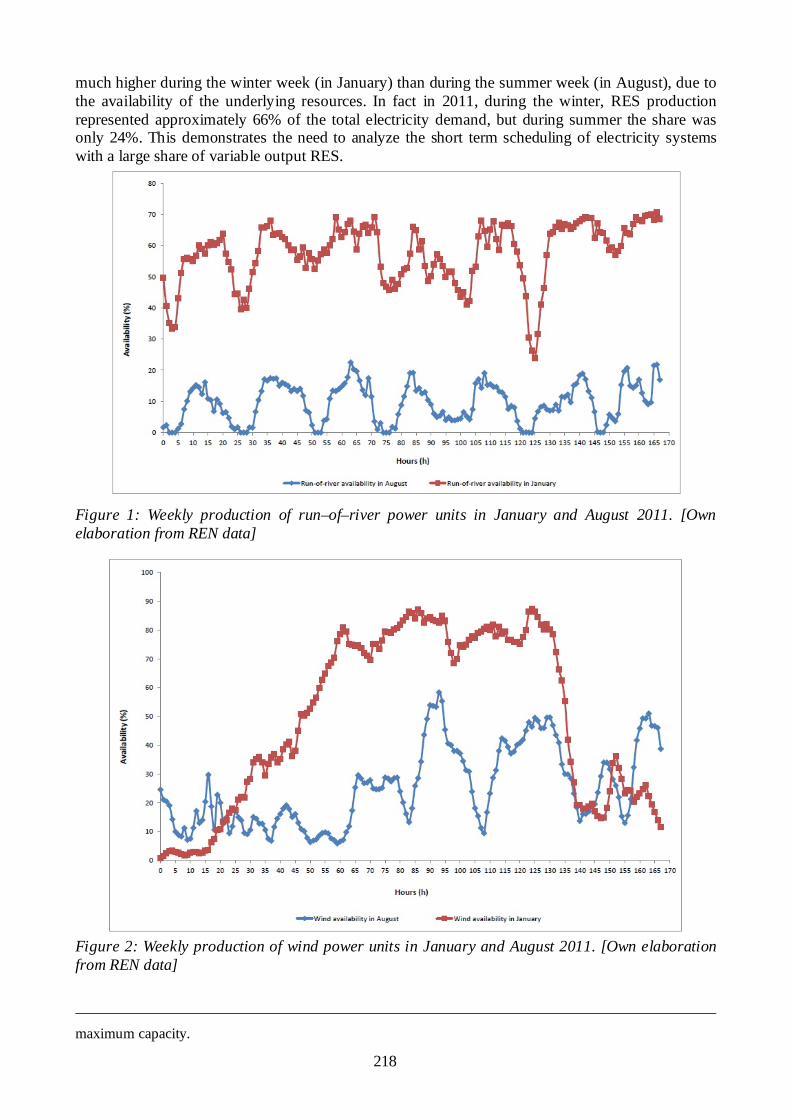
218

much higher during the winter week (in January) than during the summer week (in August), due to the availability of the underlying resources. In fact in 2011, during the winter, RES production represented approximately 66% of the total electricity demand, but during summer the share was only 24%. This demonstrates the need to analyze the short term scheduling of electricity systems with a large share of variable output RES.

Figure 1: Weekly production of run–of–river power units in January and August 2011. [Own elaboration from REN data]

Figure 2: Weekly production of wind power units in January and August 2011. [Own elaboration from REN data]

maximum capacity.

219

In the next section, numerical results corresponding to a week horizon planning are presented. A short term electricity power generation scheduling is considered for the year 2020 forecasted Portuguese system (see reference [11]).

4. Numerical results The forecasted Portuguese system over a week horizon planning for 2020 is considered in order to validate the proposed model. Considering a set of 168 hourly load blocks allow to obtain a more accurate analysis of results. In agreement with the year 2020 forecasted Portuguese system, a mix of 32 thermal power groups comprising gas, coal and fueloil technologies were considered in the model. The previously described model, represented in equations (1) to (28), originates a single objective mix integer nonlinear optimization problem (MINLP) with 11089 continuing variables, 5208 binary variables and 26016 nonlinear inequality constraints, written in the GAMS [12] modeling language. The AlphaECP [13] solver was selected to obtain the numerical results reported herein, since it proved to be the most efficient solver available. The numerical results were obtained in a Microsoft Windows operating system using a Intel core i5 processor with 4GB of memory. For simplicity, it was considered January as representative of the winter season and the August as representative of the summer season. Table 1 shows the optimal objective function values for January and August.

Table 1: Optimal objective function values Cost (M€) January August

Optimal cost 13.5 27.8 Results presented in Table 1 show that for January, the minimum cost of total power generation is lower than for August. This can easily be explained by comparing both figures A.1 and A.2 presented in Appendix A.. During the winter season, the variability of thermal power groups production is higher and the average thermal power production was 1273 MW. Also during winter, a reduction of the system variable cost is achieved, strongly dependent of the fossil fuel consumption. Nevertheless, an increase in the number of shutdowns and startups of the thermal power plants (with a direct impact on the ramping) is observed. In opposition, during summer, thermal power production remains rather steady with an average production of 3021 MW. Furthermore, no startups or shutdowns occurred, due to the low wind and hydropower production. The increase on the optimal cost is in part justified by the increase in the thermal power production during August, when compared with January. The higher summer cost is also explained by the need to fulfill the minimum up and downtime constraint of thermal power groups, in order to meet the load demand and compensate the lower wind and hydropower production. Despite the higher number of startups and shutdowns of thermal power plants in the winter season, this solution becomes less expensive due to the high availability of wind and hydropower. Thermal units are only used to compensate the lack of the RES reserves and for higher demand hours. This explains a higher wind and hydropower production with no fuel costs associated and consequently leading to a lower production cost of the entire power system.

5. Conclusions This paper analysis the short-term electricity power generation scheduling in a mixed hydro-thermal wind power system based on data close to the ones characterizing the Portuguese electricity system. A MINLP was proposed aiming to support the short term strategic decision, taking into account the

220

cost objective. The results indicate that the seasonality associated with the renewable power sources affects the behaviour of the system, and consequently its total cost. Although the electricity demand during winter increases, the higher availability of wind and hydropower production ensure that thermal power groups will remain working at a lower rate than during summer. This leads to a reduction of the variable cost of the system, strongly driven by the fuel costs. The higher number of startups and shutdowns occurred in the winter season do not necessarily reflect an increase in the system costs. The startups and shutdowns costs are in fact less relevant then the fuel cost of thermal power groups, representing 54% of the total cost of the system during winter and 0% during summer. The importance of designing short range planning models is crucial to study problems like the self-scheduling of a thermal electricity producer in day-ahead electricity markets. Future work will address the need to combine long term energy expansion strategies with short-term electrical power generation scheduling, for an hourly time step during one year horizon planning, evaluating the impact that the hydro-wind power combination strategies may have on the efficiency of thermal power plants. The model is expected to be expanded in order to increase the analysis period and to include the possibility of cross-border trading.

Acknowledgments This work was financed by: the QREN – Operational Programme for Competitiveness Factors, the European Union – European Regional Development Fund and National Funds and Portuguese Foundation for Science and Technology, under Project FCOMP-01-0124-FEDER-011377 and Project Pest-OE/EME/UI0252/2011.

Appendix A

Figure A.1: Power units production for January (week planning).

221

Figure A.2: Power units production for August (week planning).

References [1] N. Troy, E. Denny, and M. O’Malley. Base-load cycling on a system with significant wind

penetration. Power Systems, IEEE Transactions on, 25(2):1088 –1097, may 2010. [2] T. Senjyu, K. Shimabukuro, K. Uezato, and T. Funabashi. A fast technique for unit

commitment problem by extended priority list. Power Systems, IEEE Transactions on, 18(2):882 – 888, may 2003.

[3] A. ima Uyar, T. Belgin, and Ali Kele . A novel differential evolution application to short-term electrical power generation scheduling. International Journal of Electrical Power &; Energy Systems, 33(6):1236 – 1242, 2011.

[4] Thure Traber and Claudia Kemfert. Gone with the wind? electricity market prices and incentives to invest in thermal power plants under increasing wind energy supply. Energy Economics, 33(2):249 – 256, 2011.

[5] J. P. S. Catalão, S. J. P. S. Mariano, V. M. F. Mendes, and L. A. F. M. Ferreira. Short-term scheduling of thermal units: emission constraints and trade-o_ curves. European Transactions on Electrical Power, 18(1):1–14, 2008.

[6] Chao-Lung and Chiang. Optimal economic emission dispatch of hydrothermal power systems. International Journal of Electrical Power &; Energy Systems, 29(6):462 – 469, 2007.

[7] F. Hobbs. Optimization methods for electric utility resource planning. European Journal of Operational Research, 83:1–20, 1995.

[8] J. Arroyo and A. Conejo. Modelling of start-up and shut-down power trajectories of thermal units. IEEE Transactions on power systems, 19:1562–1568, 2004.

[9] WWEA. Half-year report 2011, 2011. The World Wind Energy Association. [10] REN. A energia eólica em portugal, 2010. Redes Energ´eticas Nacionais, in Portuguese. [11] S. Pereira, P. Ferreira, and A.I.F. Vaz. Electricity planning in a mixed hydro-thermal-wind

power system. submitted, 2011.

222

[12] GAMS. General Algebraic Modeling System. GAMS Corporation, 2011. http://www.gams. com.

[13] Westerlund T. and Pörn R. Solving pseudo-convex mixed integer optimization problems by cutting plane techniques. Optimization and Engineering, 3:253–280, 2002.

proceedings e report 90 · 2021. 5. 5. · ecos 2012 : the 25 th international conference on...

Documents