Processes governing natural land subsidence in the shallow coastal aquifer of the Ravenna

coast, Italy

M. Antonellini, B.M.S. Giambastiani, N. Greggio, L. Bonzi, L. Calabrese, P. Luciani,L. Perini, P. Severi

Catena Journal, 2019.

Presenter: Nguyen Thi My Tien

Advisor: Professor Chuen-Fa Ni

Date: 2020/06/121

Paper review

OUTLINE

• Introduction

➢Study area

➢Purpose

• Materials and methods

• Results and discussion

• Conclusions

2

Introduction

• Study area is located in the coastal area of the Ravenna city, in the Emilia – Romagna coastland, south of the Po River Delta (Northeastern Italy)➢ It is a lowland coastal area not

exceeding 2m above sea level.

➢Large portion below mean sea level due to effects of natural and anthropogenic land subsidence, land reclamation, and sea level rise.

3

Introduction

4

• The average rate of total land subsidence (natural + anthropogenic) in Ravenna is about 5 mm/year with the highest values recorded around the study area (values ranging from 17 to 10 mm/year).

Introduction

• Define the processes governing settlement, verify land subsidence and water table fluctuations interactions in the shallow coastal aquifer of Ravenna.

• Determine the contribution of natural processes such as primary consolidation and water table fluctuations to the cumulative land subsidence rate observed in the area.

5

Planning land subsidence management and monitoring strategies.

Purpose

Materials and methods

6

Data acquisition and elaboration

• Stage level (m) of Bevano river

• Average air temperature (℃)

• Atmospheric pressure (Pa)

• Rainfall (mm)

Settlement data (4 measurements/day)

Daily discharge

• Water table elevation (m)

• Groundwater temperature (℃)

• Salinity (g/l)

Sea level (m)

7

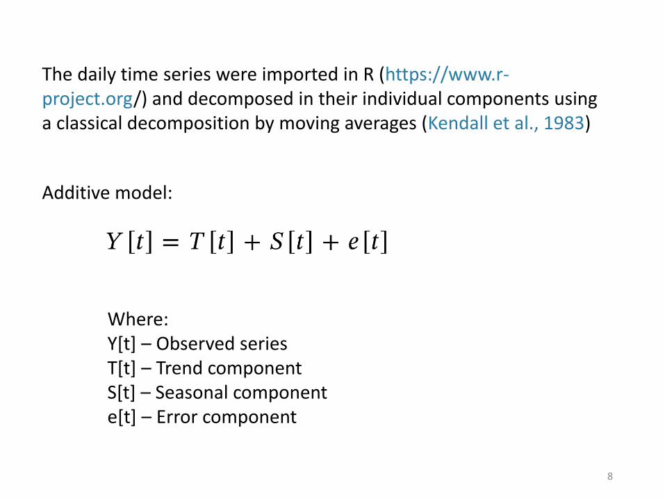
The daily time series were imported in R (https://www.r-project.org/) and decomposed in their individual components using a classical decomposition by moving averages (Kendall et al., 1983)

Where:Y[t] – Observed seriesT[t] – Trend componentS[t] – Seasonal componente[t] – Error component

Additive model:

8

Hydrogeological setting

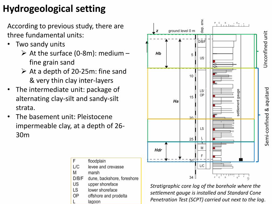
According to previous study, there are three fundamental units:• Two sandy units

➢ At the surface (0-8m): medium –fine grain sand

➢ At a depth of 20-25m: fine sand & very thin clay inter-layers

• The intermediate unit: package of alternating clay-silt and sandy-silt strata.

• The basement unit: Pleistocene impermeable clay, at a depth of 26-30m

Un

con

fin

ed u

nit

Sem

i-co

nfi

ned

& a

qu

itar

d

9

Stratigraphic core log of the borehole where the settlement gauge is installed and Standard Cone Penetration Test (SCPT) carried out next to the log.

Model construction

Time rate of consolidation and settlement

Terzaghi (1923) 1D consolidation equation

10

u: excess water pressure caused by increase of stress (Pa)t: time (days)𝑐𝑣: coefficient of consolidation

Conceptual model and boundary conditions of the system used to solve the equations of consolidation

Boundary condition: z = 0, u = 0z = 2Hdr, u = 0t = 0, u = u0

u0: initial excess fluid pore pressureHdr: equivalent thickness of all clay levels

11

The average degree of consolidation:

Settlement of clay layers:

m: summation index𝑀 = 𝜋 𝑚 + 0.5

𝑇𝑣 =𝑐𝑣. 𝑡

𝐻𝑑𝑟2

𝐻𝑖: thickness of sublayer i𝑝0(𝑖): initial effective overburden stress for sublayer i

∆𝑝0(𝑖) : increase of vertical pressure for sublayer i

𝐶𝑐: compression index usually in a range between 0.5 and 0.4 (Das, 1990). 𝑒0: initial void ratio

Effective stress in an unconfined aquifer

12

Model construction

The change of effective stress due to the water table fluctuation:

𝛾𝑠𝑎𝑡: specific weight of the saturated sediment (Pa/m)n: porosity z: topographic elevation (m)h: water table head (m)𝐻𝑎: depth of the settlement gauge (m)

Compressibility coefficient (𝑷𝒂−𝟏)

b: thickness of the aquifer∆𝑏 : variation in thickness

𝜎 : total stress (Pa)𝜎′ : effective stress (Pa)𝑢 : pore water pressure (Pa)𝐾𝑏 : bulk modulus (kg/m3)𝐾𝑠 : modulus of mineral grains (kg/m3)

Results and discussion

13

14

Time series analysis

Time series of recorded data

• At a daily level, recovery deformation is apparent in the small amplitude variations in land subsidence and water table.

15

Time series analysis

Seasonal component Noise component

• The noise components of settlement and water table are correlated

• The seasonal component of water table level, after a sharp peak, is continuously decaying (March-September)

16

• The seasonal component of land subsidence, after the March peak, has a flat top (March-June) and then decay quickly (June-September)

• The amplitude of a seasonal recoverable component in vertical displacement is about 0.89 mm.

Trend component of the settlement time series data (solid line) compared with the 1D best fit (𝑅2 = 0.99)

consolidation model (dashed line) .

Time series analysis

Magnitude of the irrecoverable consolidation rate is similar in magnitude to seasonal recoverable component.

17

0.9 mm/year

Seasonal component

Correlation coefficients between settlement and water table daily time series (blue line), and between settlement and drainage daily time series (orange line) for increasing lag time [days]

• Daily ground movement variations are related to the water table fluctuations with, eventually, a small lag in time.

• The daily water table fluctuations modify the effective stress, which inducesan almost immediate elastic response in the upper sandy portion (8-m-thick) of the coastal aquifer.

➢ This is an indication of elastic deformation in the high hydraulic conductivity (k > 5m/day) sandy part of aquifer.

18

Time series analysis

Modeling

Difference between modeled and measured land subsidence is presented in the period time (March-September).

➢ The reason for that is delayed poroelastic response of due to seepage of water in and out the prodelta of the shallow coastal aquifer

19

Average degree of consolidation (Um) for a range of consolidation coefficients values (cv) in the prodelta section above where the settlement gauge is located. The possible age of prodelta clays is reported from Amorosi et al. (1999b).

Modeling

The average degree of consolidation Um vary from 0.8 - 0.99

20

Evolution of land subsidence rates as a function of time in the shallow coastal aquifer assuming permanent settlement is due to primary consolidation of prodelta sediments only.

Modeling

21

Conclusions

• The natural land subsidence rate in the Holocene sediments of the shallow coastal aquifer accounts for 10–20% of the total land subsidence rate observed in the Ravenna area (10–20 mm/year)

22

➢ The elastic component is apparent in the daily variations of ground motion and it follows closely the water table fluctuations and has an amplitude < 0.2–0.3 mm

➢ The time-dependent delayed-elastic component of deformation isapparent in the seasonal component of land subsidence following the seasonal variations in water table, but with a time delay. The amplitude of the delayed-elastic component of deformation reaches 0.89 mm

➢ The irrecoverable component of deformation is represented by thetrend component of the land subsidence time series and it accounts for a consolidation rate of 0.9 mm/year

Thank you for your attention !

23