product validation report (pvr-13) for product h13...
TRANSCRIPT

Product Validation Report - PVR-13
(Product H13 – SN-OBS-4)
Doc.No: SAF/HSAF/PVR-13
Issue/Revision Index: 1.2.1
Date: 31/10/2012
Page: 1/46
EUMETSAT Satellite Application Facility on Support to Operational Hydrology and Water Management
Product Validation Report (PVR-13) for product H13 (SN-OBS-4)
Snow water equivalent by MW radiometry
Reference Number: SAF/HSAF/PVR-13
Issue/Revision Index: 1.2.1
Last Change: 21 November 2012
About this document This Document has been prepared by the Product Validation Cluster Leader, with the support of the Project Management Team and of the Validation and Development Teams of the Snow Cluster

Product Validation Report - PVR-13
(Product H13 – SN-OBS-4)
Doc.No: SAF/HSAF/PVR-13
Issue/Revision Index: 1.2.1
Date: 31/10/2012
Page: 2/46
DOCUMENT CHANGE RECORD
Issue / Revision Date Description
1.0 20/01/2012 Baseline version prepared for ORR1 Part 3.
1.1 31/05/2012
Updated release for CDOP2 ORR1 Part3 Close-out:
General revision, removal of duplicates, addition of required information (RID1)
Insertion of explanation on SWE estimate interpolation (RID3) in the new section 3.6.2
Clarification on significance of the Turkish case study, at the end of section 4.3 (RID4)
Correction of editorial errors (RID12)
Correction of references to product requirements (RID 2 on PVR14)
1.2 31/10/2012 Updated release for CDOP2 ORR1 Part3 Close-out 2: updated sections 2.1, 5.*, 6.* and 7.* .
1.2.1 21/11/2012 Section 6.4 removed; Section 6.5 moved to section 6.4

Product Validation Report - PVR-13
(Product H13 – SN-OBS-4)
Doc.No: SAF/HSAF/PVR-13
Issue/Revision Index: 1.2.1
Date: 31/10/2012
Page: 3/46
Index
1 The EUMETSAT Satellite Application Facilities and H-SAF ........................................................................ 7 2 Introduction to product SN-OBS-4 ............................................................................................................ 9
2.1 Sensing principle ................................................................................................................................ 9 2.2 Algorithm principle .......................................................................................................................... 11 2.3 Main operational characteristics ..................................................................................................... 13
3 Validation strategy, methods and tools .................................................................................................. 15 3.1 Validation team and work plan ....................................................................................................... 15 3.2 Validation objects and problems ..................................................................................................... 16 3.3 Validation methodology .................................................................................................................. 17 3.4 Observation data ............................................................................................................................. 17 3.5 Data consistency check .................................................................................................................... 17 3.6 Comparison between the observation data and the product ......................................................... 18
3.6.1 Comparison for Flat/Forest Areas ................................................................................ 18
3.6.2 The SWE estimate ........................................................................................................ 18
3.6.3 Comparison for Mountainous areas ............................................................................ 20 3.7 Definition of statistical scores ......................................................................................................... 22
3.7.1 Scores for continuous statistics ................................................................................... 22
3.7.2 Scores for dichotomous statistics ................................................................................ 23 4 Ground data used for validation activities .............................................................................................. 25
4.1 Ground data in Finland (FMI) .......................................................................................................... 25
4.1.1 Snow Measurement Courses ....................................................................................... 26
4.1.2 Hydrological simulation and forecasting system ......................................................... 26
4.1.3 The Sodankylä-Pallas validation region ....................................................................... 27 4.2 Ground data in Turkey (ITU) ............................................................................................................ 27
5 Validation results: case study analysis .................................................................................................... 30 5.1 Case Studies in Turkey ..................................................................................................................... 30
5.1.1 Case study for 09.02.2010 ........................................................................................... 30
5.1.2 Case study for 12.03.2011 ........................................................................................... 31 6 Validation results: long statistic analysis................................................................................................. 33
6.1 Introduction ..................................................................................................................................... 33 6.2 Validation exercises in Turkey ......................................................................................................... 33 6.3 Validation with synoptic weather station data ............................................................................... 33 6.4 Validation results in Finland ............................................................................................................ 37 6.5 Some conclusions ............................................................................................................................ 38
7 Conclusions ............................................................................................................................................. 40 7.1 Summary conclusions on product validation .................................................................................. 40
8 Reference documents ............................................................................................................................. 41 Annex 1. Validation methodology for H13 – Snow water equivalent ........................................................ 42 Annex 2. Mountainous Area Mask Determination for HSAF Project ......................................................... 46

Product Validation Report - PVR-13
(Product H13 – SN-OBS-4)
Doc.No: SAF/HSAF/PVR-13
Issue/Revision Index: 1.2.1
Date: 31/10/2012
Page: 4/46
List of tables
Table 1 H-SAF Product List ................................................................................................................................. 8 Table 2 Current status of the EOS-Aqua satellite and DMSP-satellites (as of January 2012) ........................ 10 Table 3 Main features of AMSR-E and SSMI/S ................................................................................................ 11 Table 4 Validation team of H-SAF snow products ........................................................................................... 15 Table 5 Areal average SWE values obtained from H13 and hydrological model HBV for Karasu basin ......... 31 Table 6 Accuracy requirements for product PR-OBS-13 [RMSE] ..................................................................... 33 Table 7 Results for validation period January, 2010 – March, 2010 ............................................................. 34 Table 8 Accuracy table for validation period January, 2011 – March, 2011 ................................................... 35 Table 9 Accuracy table for validation period January, 2012 – March, 2012 ................................................... 36 Table 10 Simplified compliance analysis for product H13............................................................................... 39 Table 11 H-SAF Accuracy requirements for H13 [RMSE] ................................................................................ 39 Table 12 Land use/cover classes in mountainous areas ................................................................................. 46
List of figures
Figure 1 Conceptual scheme of the EUMETSAT application ground segment .................................................. 7 Figure 2 Current composition of the EUMETSAT SAF network (in order of establishment) ............................. 7 Figure 3 Geometry of conical scanning for AMSR-E ......................................................................................... 9 Figure 4 Mask flat/forested versus mountainous regions .............................................................................. 10 Figure 5 Flow diagram of the assimilation method, case of AMSR-E observations in flat/forested areas ..... 12 Figure 6 Flow diagram of the assimilation method, case of AMSR-E observations in mountainous areas .... 13 Figure 7 Structure of the Snow products validation team .............................................................................. 15 Figure 8 SWE estimate: difference between assimilated value and background field – difference map for 15/03/1993 (single day estimate) ................................................................................................................... 19 Figure 9 SWE estimate: difference between assimilated value and background field – histogram for complete dataset from 1982 to 2009 .............................................................................................................. 19 Figure 10 Snow measurement courses (SYKE) and weather stations (FMI) in Finland ................................... 25 Figure 11 SCA from SYKE watershed simulation and forecasting system (WSFS) ........................................... 26 Figure 12 Land cover map of the Sodankylä-Pallas site .................................................................................. 27 Figure 13 H13 product for February 9, 2010 ................................................................................................... 30 Figure 14 H13 product masked with H13 product for February 9, 2010 ........................................................ 30 Figure 15 H13 product for March 12, 2011 ..................................................................................................... 31 Figure 16 H13 product masked with H13 product for March 12, 2011 .......................................................... 31 Figure 17 TSMS synoptic, climate and AWOS stations reporting snow depths .............................................. 34 Figure 18 The calculated mean snow water equivalent obtained from H13 corresponding to measured snow water equivalent values for the period January, 2010 – March, 2010 ........................................................... 35 Figure 19 The calculated mean snow water equivalent values obtained from H13 corresponding to measured snow water equivalent values for the period January, 2011 – March, 2011 ................................. 36 Figure 20 The calculated mean snow water equivalent values obtained from H13 corresponding to measured snow water equivalent values for the period January, 2012 – March, 2012 .............................. 37 Figure 21 validation results in Finland ............................................................................................................. 38

Product Validation Report - PVR-13
(Product H13 – SN-OBS-4)
Doc.No: SAF/HSAF/PVR-13
Issue/Revision Index: 1.2.1
Date: 31/10/2012
Page: 5/46
Acronyms
AMSU Advanced Microwave Sounding Unit (on NOAA and MetOp)
AMSU-A Advanced Microwave Sounding Unit - A (on NOAA and MetOp)
AMSU-B Advanced Microwave Sounding Unit - B (on NOAA up to 17)
ATDD Algorithms Theoretical Definition Document
AU Anadolu University (in Turkey)
BfG Bundesanstalt für Gewässerkunde (in Germany)
CAF Central Application Facility (of EUMETSAT)
CDOP Continuous Development-Operations Phase
CESBIO Centre d'Etudes Spatiales de la BIOsphere (of CNRS, in France)
CM-SAF SAF on Climate Monitoring
CNMCA Centro Nazionale di Meteorologia e Climatologia Aeronautica (in Italy)
CNR Consiglio Nazionale delle Ricerche (of Italy)
CNRS Centre Nationale de la Recherche Scientifique (of France)
DMSP Defense Meteorological Satellite Program
DPC Dipartimento Protezione Civile (of Italy)
EARS EUMETSAT Advanced Retransmission Service
ECMWF European Centre for Medium-range Weather Forecasts
EDC EUMETSAT Data Centre, previously known as U-MARF
EUM Short for EUMETSAT
EUMETCast EUMETSAT’s Broadcast System for Environmental Data
EUMETSAT European Organisation for the Exploitation of Meteorological Satellites
FMI Finnish Meteorological Institute
FTP File Transfer Protocol
GEO Geostationary Earth Orbit
GRAS-SAF SAF on GRAS Meteorology
HDF Hierarchical Data Format
HRV High Resolution Visible (one SEVIRI channel)
H-SAF SAF on Support to Operational Hydrology and Water Management
IDL©
Interactive Data Language
IFOV Instantaneous Field Of View
IMWM Institute of Meteorology and Water Management (in Poland)
IPF Institut für Photogrammetrie und Fernerkundung (of TU-Wien, in Austria)
IPWG International Precipitation Working Group
IR Infra Red
IRM Institut Royal Météorologique (of Belgium) (alternative of RMI)
ISAC Istituto di Scienze dell’Atmosfera e del Clima (of CNR, Italy)
ITU İstanbul Technical University (in Turkey)
LATMOS Laboratoire Atmosphères, Milieux, Observations Spatiales (of CNRS, in France)
LEO Low Earth Orbit
LSA-SAF SAF on Land Surface Analysis
Météo France National Meteorological Service of France
METU Middle East Technical University (in Turkey)
MHS Microwave Humidity Sounder (on NOAA 18 and 19, and on MetOp)
MSG Meteosat Second Generation (Meteosat 8, 9, 10, 11)
MVIRI Meteosat Visible and Infra Red Imager (on Meteosat up to 7)
MW Micro Wave
NESDIS National Environmental Satellite, Data and Information Services
NMA National Meteorological Administration (of Romania)
NOAA National Oceanic and Atmospheric Administration (Agency and satellite)
Product Validation Report - PVR-13
(Product H13 – SN-OBS-4)
Doc.No: SAF/HSAF/PVR-13
Issue/Revision Index: 1.2.1
Date: 31/10/2012
Page: 6/46
NWC-SAF SAF in support to Nowcasting & Very Short Range Forecasting
NWP Numerical Weather Prediction
NWP-SAF SAF on Numerical Weather Prediction
O3M-SAF SAF on Ozone and Atmospheric Chemistry Monitoring
OMSZ Hungarian Meteorological Service
ORR Operations Readiness Review
OSI-SAF SAF on Ocean and Sea Ice
PDF Probability Density Function
PEHRPP Pilot Evaluation of High Resolution Precipitation Products
Pixel Picture element
PMW Passive Micro-Wave
PP Project Plan
PR Precipitation Radar (on TRMM)
PRD Product Requirement Document
PUM Product User Manual
PVR Product Validation Report
RMI Royal Meteorological Institute (of Belgium) (alternative of IRM)
RR Rain Rate
RU Rapid Update
SAF Satellite Application Facility
SEVIRI Spinning Enhanced Visible and Infra-Red Imager (on Meteosat from 8 onwards)
SHMÚ Slovak Hydro-Meteorological Institute
SSM/I Special Sensor Microwave / Imager (on DMSP up to F-15)
SSMIS Special Sensor Microwave Imager/Sounder (on DMSP starting with S-16)
SYKE Suomen ympäristökeskus (Finnish Environment Institute)
TBB Equivalent Blackbody Temperature (used for IR)
TKK Teknillinen korkeakoulu (Helsinki University of Technology)
TMI TRMM Microwave Imager (on TRMM)
TRMM Tropical Rainfall Measuring Mission UKMO
TSMS Turkish State Meteorological Service
TU-Wien Technische Universität Wien (in Austria)
U-MARF Unified Meteorological Archive and Retrieval Facility
UniFe University of Ferrara (in Italy)
UTC Universal Coordinated Time
VIS Visible
ZAMG Zentralanstalt für Meteorologie und Geodynamik (of Austria)
Product Validation Report - PVR-13
(Product H13 – SN-OBS-4)
Doc.No: SAF/HSAF/PVR-13
Issue/Revision Index: 1.2.1
Date: 31/10/2012
Page: 7/46
1 The EUMETSAT Satellite Application Facilities and H-SAF
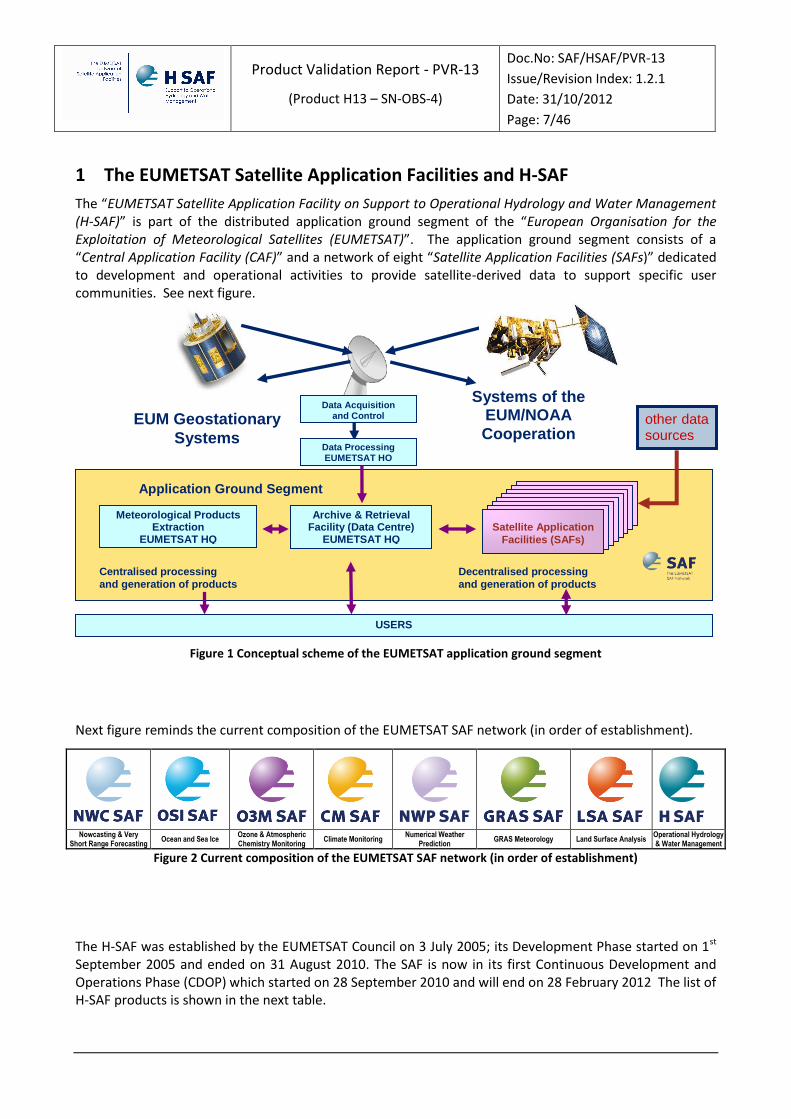
The “EUMETSAT Satellite Application Facility on Support to Operational Hydrology and Water Management (H-SAF)” is part of the distributed application ground segment of the “European Organisation for the Exploitation of Meteorological Satellites (EUMETSAT)”. The application ground segment consists of a “Central Application Facility (CAF)” and a network of eight “Satellite Application Facilities (SAFs)” dedicated to development and operational activities to provide satellite-derived data to support specific user communities. See next figure.
Figure 1 Conceptual scheme of the EUMETSAT application ground segment
Next figure reminds the current composition of the EUMETSAT SAF network (in order of establishment).
Nowcasting & Very
Short Range Forecasting Ocean and Sea Ice Ozone & Atmospheric Chemistry Monitoring Climate Monitoring Numerical Weather
Prediction GRAS Meteorology Land Surface Analysis Operational Hydrology
& Water Management Figure 2 Current composition of the EUMETSAT SAF network (in order of establishment)
The H-SAF was established by the EUMETSAT Council on 3 July 2005; its Development Phase started on 1st September 2005 and ended on 31 August 2010. The SAF is now in its first Continuous Development and Operations Phase (CDOP) which started on 28 September 2010 and will end on 28 February 2012 The list of H-SAF products is shown in the next table.
Decentralised processing
and generation of products
EUM Geostationary
Systems
Systems of the EUM/NOAA
Cooperation
Centralised processing
and generation of products
Data Acquisition and Control
Data Processing EUMETSAT HQ
Meteorological Products Extraction
EUMETSAT HQ
Archive & Retrieval Facility (Data Centre)
EUMETSAT HQ
USERS
Application Ground Segment
other data sources
Satellite Application
Facilities (SAFs)

Product Validation Report - PVR-13
(Product H13 – SN-OBS-4)
Doc.No: SAF/HSAF/PVR-13
Issue/Revision Index: 1.2.1
Date: 31/10/2012
Page: 8/46
Acronym Identifier Name
PR-OBS-1 H-01 Precipitation rate at ground by MW conical scanners (with indication of phase)
PR-OBS-2 H-02 Precipitation rate at ground by MW cross-track scanners (with indication of phase)
PR-OBS-3 H-03 Precipitation rate at ground by GEO/IR supported by LEO/MW
PR-OBS-4 H-04 Precipitation rate at ground by LEO/MW supported by GEO/IR (with flag for phase)
PR-OBS-5 H-05 Accumulated precipitation at ground by blended MW and IR
PR-OBS-6 H-15 Blended SEVIRI Convection area/ LEO MW Convective Precipitation
PR-ASS-1 H-06 Instantaneous and accumulated precipitation at ground computed by a NWP model
SM-OBS-2 H-08 Small-scale surface soil moisture by radar scatterometer
SM-OBS-3 H-16 Large-scale surface soil moisture by radar scatterometer
SM-DAS-2 H-14 Soil Moisture profile index in the roots region by scatterometer assimilation method
SN-OBS-1 H-10 Snow detection (snow mask) by VIS/IR radiometry
SN-OBS-2 H-11 Snow status (dry/wet) by MW radiometry
SN-OBS-3 H-12 Effective snow cover by VIS/IR radiometry
SN-OBS-4 H-13 Snow water equivalent by MW radiometry
Table 1 H-SAF Product List
Product Validation Report - PVR-13
(Product H13 – SN-OBS-4)
Doc.No: SAF/HSAF/PVR-13
Issue/Revision Index: 1.2.1
Date: 31/10/2012
Page: 9/46
2 Introduction to product SN-OBS-4
2.1 Sensing principle
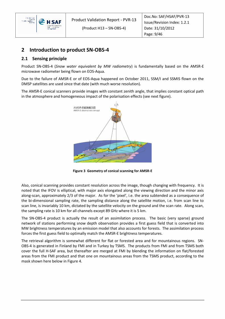
Product SN-OBS-4 (Snow water equivalent by MW radiometry) is fundamentally based on the AMSR-E microwave radiometer being flown on EOS-Aqua.
Due to the failure of AMSR-E or of EOS-Aqua happened on October 2011, SSM/I and SSMIS flown on the DMSP satellites are used since that date (with much worse resolution).
The AMSR-E conical scanners provide images with constant zenith angle, that implies constant optical path in the atmosphere and homogeneous impact of the polarisation effects (see next figure).
Figure 3 Geometry of conical scanning for AMSR-E
Also, conical scanning provides constant resolution across the image, though changing with frequency. It is noted that the IFOV is elliptical, with major axis elongated along the viewing direction and the minor axis along-scan, approximately 2/3 of the major. As for the ‘pixel’, i.e. the area subtended as a consequence of the bi-dimensional sampling rate, the sampling distance along the satellite motion, i.e. from scan line to scan line, is invariably 10 km, dictated by the satellite velocity on the ground and the scan rate. Along scan, the sampling rate is 10 km for all channels except 89 GHz where it is 5 km.
The SN-OBS-4 product is actually the result of an assimilation process. The basic (very sparse) ground network of stations performing snow depth observation provides a first guess field that is converted into MW brightness temperatures by an emission model that also accounts for forests. The assimilation process forces the first guess field to optimally match the AMSR-E brightness temperatures.
The retrieval algorithm is somewhat different for flat or forested area and for mountainous regions. SN-OBS-4 is generated in Finland by FMI and in Turkey by TSMS. The products from FMI and from TSMS both cover the full H-SAF area, but thereafter are merged at FMI by blending the information on flat/forested areas from the FMI product and that one on mountainous areas from the TSMS product, according to the mask shown here below in Figure 4.
Product Validation Report - PVR-13
(Product H13 – SN-OBS-4)
Doc.No: SAF/HSAF/PVR-13
Issue/Revision Index: 1.2.1
Date: 31/10/2012
Page: 10/46
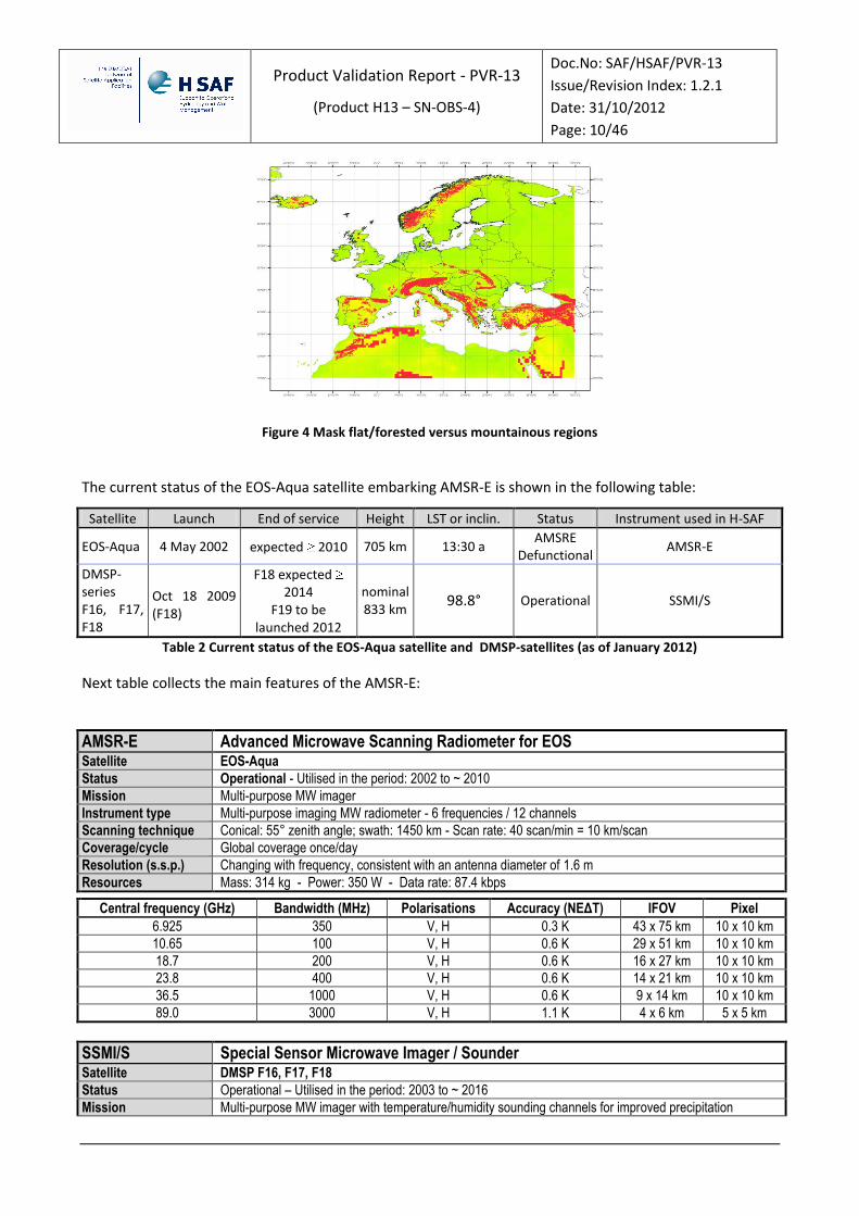
Figure 4 Mask flat/forested versus mountainous regions
The current status of the EOS-Aqua satellite embarking AMSR-E is shown in the following table:
Satellite Launch End of service Height LST or inclin. Status Instrument used in H-SAF
EOS-Aqua 4 May 2002 expected 2010 705 km 13:30 a AMSRE
Defunctional AMSR-E
DMSP-series F16, F17, F18
Oct 18 2009 (F18)
F18 expected 2014
F19 to be launched 2012
nominal 833 km
98.8° Operational SSMI/S
Table 2 Current status of the EOS-Aqua satellite and DMSP-satellites (as of January 2012)
Next table collects the main features of the AMSR-E:
AMSR-E Advanced Microwave Scanning Radiometer for EOS Satellite EOS-Aqua
Status Operational - Utilised in the period: 2002 to ~ 2010
Mission Multi-purpose MW imager
Instrument type Multi-purpose imaging MW radiometer - 6 frequencies / 12 channels
Scanning technique Conical: 55° zenith angle; swath: 1450 km - Scan rate: 40 scan/min = 10 km/scan
Coverage/cycle Global coverage once/day
Resolution (s.s.p.) Changing with frequency, consistent with an antenna diameter of 1.6 m
Resources Mass: 314 kg - Power: 350 W - Data rate: 87.4 kbps
Central frequency (GHz) Bandwidth (MHz) Polarisations Accuracy (NEΔT) IFOV Pixel
6.925 350 V, H 0.3 K 43 x 75 km 10 x 10 km
10.65 100 V, H 0.6 K 29 x 51 km 10 x 10 km
18.7 200 V, H 0.6 K 16 x 27 km 10 x 10 km
23.8 400 V, H 0.6 K 14 x 21 km 10 x 10 km
36.5 1000 V, H 0.6 K 9 x 14 km 10 x 10 km
89.0 3000 V, H 1.1 K 4 x 6 km 5 x 5 km
SSMI/S Special Sensor Microwave Imager / Sounder Satellite DMSP F16, F17, F18
Status Operational – Utilised in the period: 2003 to ~ 2016
Mission Multi-purpose MW imager with temperature/humidity sounding channels for improved precipitation
Product Validation Report - PVR-13
(Product H13 – SN-OBS-4)
Doc.No: SAF/HSAF/PVR-13
Issue/Revision Index: 1.2.1
Date: 31/10/2012
Page: 11/46
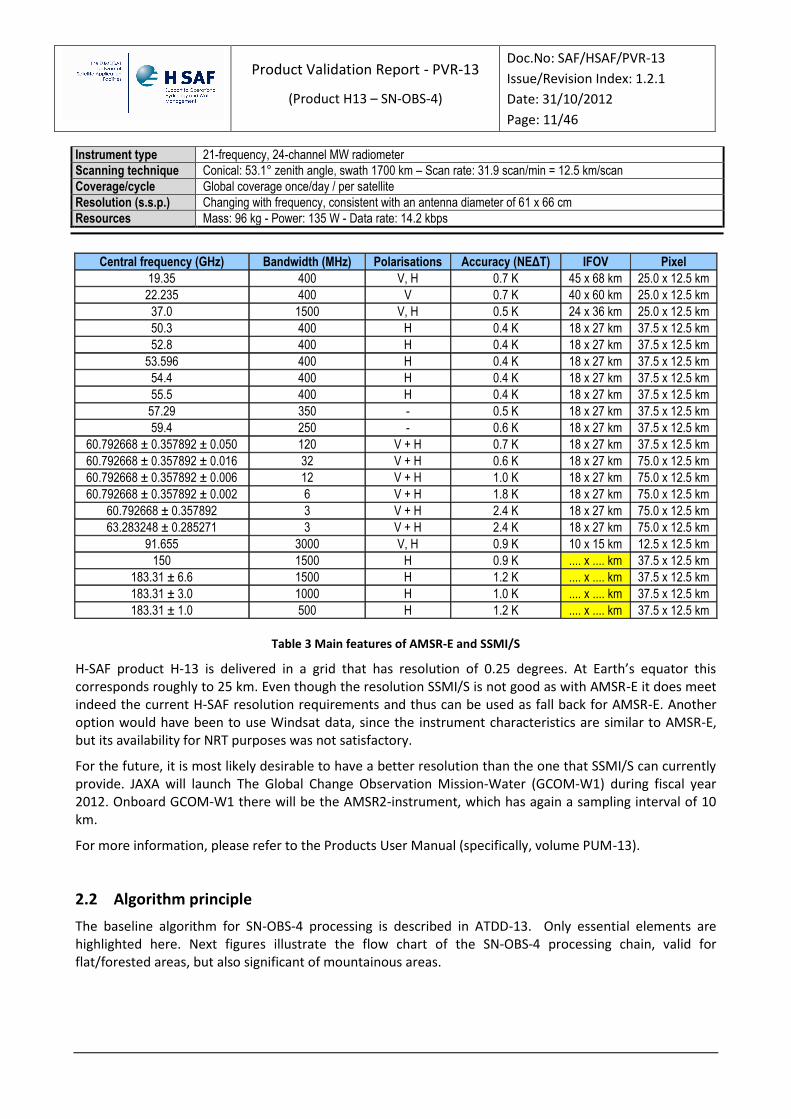
Instrument type 21-frequency, 24-channel MW radiometer
Scanning technique Conical: 53.1° zenith angle, swath 1700 km – Scan rate: 31.9 scan/min = 12.5 km/scan
Coverage/cycle Global coverage once/day / per satellite
Resolution (s.s.p.) Changing with frequency, consistent with an antenna diameter of 61 x 66 cm
Resources Mass: 96 kg - Power: 135 W - Data rate: 14.2 kbps
Central frequency (GHz) Bandwidth (MHz) Polarisations Accuracy (NEΔT) IFOV Pixel
19.35 400 V, H 0.7 K 45 x 68 km 25.0 x 12.5 km
22.235 400 V 0.7 K 40 x 60 km 25.0 x 12.5 km
37.0 1500 V, H 0.5 K 24 x 36 km 25.0 x 12.5 km
50.3 400 H 0.4 K 18 x 27 km 37.5 x 12.5 km
52.8 400 H 0.4 K 18 x 27 km 37.5 x 12.5 km
53.596 400 H 0.4 K 18 x 27 km 37.5 x 12.5 km
54.4 400 H 0.4 K 18 x 27 km 37.5 x 12.5 km
55.5 400 H 0.4 K 18 x 27 km 37.5 x 12.5 km
57.29 350 - 0.5 K 18 x 27 km 37.5 x 12.5 km
59.4 250 - 0.6 K 18 x 27 km 37.5 x 12.5 km
60.792668 ± 0.357892 ± 0.050 120 V + H 0.7 K 18 x 27 km 37.5 x 12.5 km
60.792668 ± 0.357892 ± 0.016 32 V + H 0.6 K 18 x 27 km 75.0 x 12.5 km
60.792668 ± 0.357892 ± 0.006 12 V + H 1.0 K 18 x 27 km 75.0 x 12.5 km
60.792668 ± 0.357892 ± 0.002 6 V + H 1.8 K 18 x 27 km 75.0 x 12.5 km
60.792668 ± 0.357892 3 V + H 2.4 K 18 x 27 km 75.0 x 12.5 km
63.283248 ± 0.285271 3 V + H 2.4 K 18 x 27 km 75.0 x 12.5 km
91.655 3000 V, H 0.9 K 10 x 15 km 12.5 x 12.5 km
150 1500 H 0.9 K .... x .... km 37.5 x 12.5 km
183.31 ± 6.6 1500 H 1.2 K .... x .... km 37.5 x 12.5 km
183.31 ± 3.0 1000 H 1.0 K .... x .... km 37.5 x 12.5 km
183.31 ± 1.0 500 H 1.2 K .... x .... km 37.5 x 12.5 km
Table 3 Main features of AMSR-E and SSMI/S
H-SAF product H-13 is delivered in a grid that has resolution of 0.25 degrees. At Earth’s equator this corresponds roughly to 25 km. Even though the resolution SSMI/S is not good as with AMSR-E it does meet indeed the current H-SAF resolution requirements and thus can be used as fall back for AMSR-E. Another option would have been to use Windsat data, since the instrument characteristics are similar to AMSR-E, but its availability for NRT purposes was not satisfactory.
For the future, it is most likely desirable to have a better resolution than the one that SSMI/S can currently provide. JAXA will launch The Global Change Observation Mission-Water (GCOM-W1) during fiscal year 2012. Onboard GCOM-W1 there will be the AMSR2-instrument, which has again a sampling interval of 10 km.
For more information, please refer to the Products User Manual (specifically, volume PUM-13).
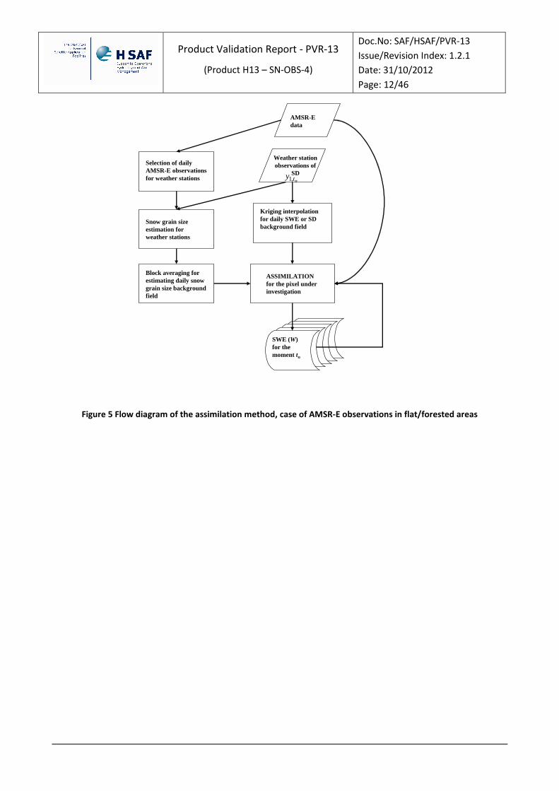
2.2 Algorithm principle
The baseline algorithm for SN-OBS-4 processing is described in ATDD-13. Only essential elements are highlighted here. Next figures illustrate the flow chart of the SN-OBS-4 processing chain, valid for flat/forested areas, but also significant of mountainous areas.
Product Validation Report - PVR-13
(Product H13 – SN-OBS-4)
Doc.No: SAF/HSAF/PVR-13
Issue/Revision Index: 1.2.1
Date: 31/10/2012
Page: 12/46
AMSR-E
data
Weather station
observations of
SD
Selection of daily
AMSR-E observations
for weather stations
Snow grain size
estimation for
weather stations
Kriging interpolation
for daily SWE or SD
background field
Block averaging for
estimating daily snow
grain size background
field
ASSIMILATION
for the pixel under
investigation
SWE (W)
for the
moment tn
WtnW ,ˆ
1
nty ,1
nty ,1
nn tWtW ,ref,,ref ,ˆ
ntW
n
n
td
td
ref,,0
ref,,0ˆ
Figure 5 Flow diagram of the assimilation method, case of AMSR-E observations in flat/forested areas
Product Validation Report - PVR-13
(Product H13 – SN-OBS-4)
Doc.No: SAF/HSAF/PVR-13
Issue/Revision Index: 1.2.1
Date: 31/10/2012
Page: 13/46
AMSR-E Level1A 10.7,18.7 &
36.5 GHz Vertical and Horizontal
Polarization Channel Data
Projecting Tb(Brightness Temperatures) of 10.7,
18.7 & 36.5 Vertical and Horizontal Channels to
0.25 Degree Spatial Resolution Geographic Grid.
SD estimation for pixel in
between 5cm to 100 cm.
estimating daily snow
grain size (d0)
background field
)( 0db
b
aeT
SD
Estimation of daily snow
density( ) background
fieldyxd5
0
Assimilation for the pixel under
investigation
Snow Water
Equivalent SWE of
the pixel
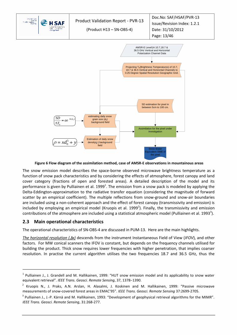
Figure 6 Flow diagram of the assimilation method, case of AMSR-E observations in mountainous areas
The snow emission model describes the space-borne observed microwave brightness temperature as a function of snow pack characteristics and by considering the effects of atmosphere, forest canopy and land cover category (fractions of open and forested areas). A detailed description of the model and its performance is given by Pulliainen et al. 19991. The emission from a snow pack is modeled by applying the Delta-Eddington-approximation to the radiative transfer equation (considering the magnitude of forward scatter by an empirical coefficient). The multiple reflections from snow-ground and snow-air boundaries are included using a non-coherent approach and the effect of forest canopy (transmissivity and emission) is included by employing an empirical model (Kruopis et al. 19992). Finally, the transmissivity and emission contributions of the atmosphere are included using a statistical atmospheric model (Pulliainen et al. 19933).
2.3 Main operational characteristics
The operational characteristics of SN-OBS-4 are discussed in PUM-13. Here are the main highlights.
The horizontal resolution ( x) descends from the instrument Instantaneous Field of View (IFOV), and other factors. For MW conical scanners the IFOV is constant, but depends on the frequency channels utilised for building the product. Thick snow requires lower frequencies with higher penetration, that implies coarser resolution. In practise the current algorithm utilises the two frequencies 18.7 and 36.5 GHz, thus the
1 Pulliainen J., J. Grandell and M. Hallikainen, 1999: “HUT snow emission model and its applicability to snow water
equivalent retrieval”. IEEE Trans. Geosci. Remote Sensing, 37, 1378−1390. 2 Kruopis N., J. Praks, A.N. Arslan, H. Alasalmi, J. Koskinen and M. Hallikainen, 1999: “Passive microwave
measurements of snow-covered forest areas in EMAC’95”. IEEE Trans. Geosci. Remote Sensing 37:2699-2705. 3 Pulliainen J., J.-P. Kärnä and M. Hallikainen, 1993: “Development of geophysical retrieval algorithms for the MIMR”.
IEEE Trans. Geosci. Remote Sensing, 31:268-277.

Product Validation Report - PVR-13
(Product H13 – SN-OBS-4)
Doc.No: SAF/HSAF/PVR-13
Issue/Revision Index: 1.2.1
Date: 31/10/2012
Page: 14/46
resolution is that one of AMSR-E at 18.7 GHz, i.e. ~ 20 km. Sampling also is made at ~ 20 km intervals (0.25°). Conclusion for PR-OBS-4:
resolution: x ~ 20 km - sampling distance: ~ 20 km.
The observing cycle ( t). AMSR-E is available only on one satellite, and its swath is 1450 km, thus in principle provides global coverage every 24 h. Conclusion:
observing cycle: t = 24 h.
The timeliness ( ) is defined as the time between observation taking and product available at the user site assuming a defined dissemination mean. For a product resulting by assembling data collected until a fixed time of the day, the time of observation may change across the scene (some area may have been observed early in the time window, thus up to 24-h old at the time of dissemination; some very recently, just before product dissemination). The average delay is therefore δ = 12 h. Conclusion:
timeliness: ~ 12 h.
The accuracy (RMS) is the convolution of several measurement features (random error, bias, sensitivity, precision, …). To simplify matters, it is generally agreed to quote the root-mean-square difference [observed - true values]. The accuracy of a satellite-derived product descends from the strength of the physical principle linking the satellite observation to the natural process determining the parameter. It is difficult to estimate a-priori: it is generally evaluated a-posteriori by means of the validation activity.
Product Validation Report - PVR-13
(Product H13 – SN-OBS-4)
Doc.No: SAF/HSAF/PVR-13
Issue/Revision Index: 1.2.1
Date: 31/10/2012
Page: 15/46
3 Validation strategy, methods and tools
3.1 Validation team and work plan
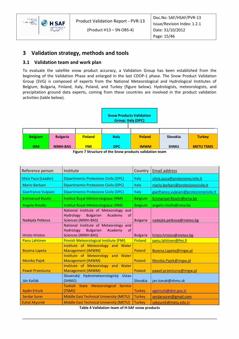
To evaluate the satellite snow product accuracy, a Validation Group has been established from the beginning of the Validation Phase and enlarged in the last CDOP-1 phase. The Snow Product Validation Group (SVG) is composed of experts from the National Meteorological and Hydrological Institutes of Belgium, Bulgaria, Finland, Italy, Poland, and Turkey (figure below). Hydrologists, meteorologists, and precipitation ground data experts, coming from these countries are involved in the product validation activities (table below).
Figure 7 Structure of the Snow products validation team
Snow Products Validation Group: Italy (DPC)
Belgium
IRM
Bulgaria
NIMH-BAS
Finland
FMI
Italy
DPC
Poland
IMWM
Slovakia
SHMU
Turkey
METU TSMS
Reference person Institute Country Email address
Silvia Puca (Leader) Dipartimento Protezione Civile (DPC) Italy [email protected]
Mario Barbani Dipartimento Protezione Civile (DPC) Italy [email protected]
Gianfranco Vulpiani Dipartimento Protezione Civile (DPC) Italy [email protected]
Emmanuel Roulin Institut Royal Météorologique (IRM) Belgium [email protected]
Angelo Rinollo Institut Royal Météorologique (IRM) Belgium [email protected]
Nadejda Petkova
National Institute of Meteorology and Hydrology Bulgarian Academy of Sciences (NIMH-BAS) Bulgaria [email protected]
Hristo Hristov
National Institute of Meteorology and Hydrology Bulgarian Academy of Sciences (NIMH-BAS) Bulgaria [email protected]
Panu Lahtinen Finnish Meteorological Institute (FMI) Finland [email protected]
Bozena Lapeta Institute of Meteorology and Water Management (IMWM) Poland [email protected]
Monika Pajek Institute of Meteorology and Water Management (IMWM) Poland [email protected]
Pawel Przeniczny Institute of Meteorology and Water Management (IMWM) Poland [email protected]
Ján Kaňák Slovenský Hydrometeorologický Ústav (SHMÚ) Slovakia [email protected]
Aydin Erturk Turkish State Meteorological Service (TSMS) Turkey [email protected]
Serdar Surer Middle East Technical University (METU) Turkey [email protected]
Zuhal Akyurek Middle East Technical University (METU) Turkey [email protected]
Table 4 Validation team of H-SAF snow products

Product Validation Report - PVR-13
(Product H13 – SN-OBS-4)
Doc.No: SAF/HSAF/PVR-13
Issue/Revision Index: 1.2.1
Date: 31/10/2012
Page: 16/46
The participants to the Validation group do not only validate the products: they also define the validation method, the data to be used and the development of validation tools. Two Institutes, FMI in Finland and METU in Turkey have been using their own data for validation of this product, but all the institutes have been working in the validation procedure. There are lots of snow depth (SD) measurements available in Europe, also in other countries, but they can’t be used in the validation of this product, since SD data is used as input in generating the snow product. Another issue is that point-wise snow depth measurements do not adequately represent the whole pixel in H-SAF H13 grid (0.25° x 0.25°). Only independent snow course measurements can be used as reliable validation data and such data are not generally available for flat areas, except for Finland, where the Finnish Environment Institute provides independent SWE measurements from snow courses. Regarding SWE for mountainous areas, the validation results of space borne SWE depend on the availability of snow depth and snow water equivalent measurements on the ground. Since no ancillary data is used in retrieval of SWE from microwave data, all the available SD and SWE observations can be used in the validation. But the problem is the availability of the SD and SWE measurements in mountainous areas. The scarcity of observations and the rough terrain make the observations of SWE and SD more difficult and less dependable in mountainous areas. In addition, the procedure of excluding weather station or ground measurement from validation studies, if the elevation difference between its location and the AMSR-E pixel median elevation inside which the measurement falls is greater than 400 meters (see 3.6.3), limits the number of ground observations that can be used in validation (elevation range of ground reference data is from 981 meters to 2937 meters in Turkey validation study). The Snow products validation programme was started during the development phase of the project and was finalised during the last H-SAF Products and Hydro Validation Workshop hosted by Italian Civil Protection in Rome, 29 of November - 2 of December 2011. A snow product validation section of the H-SAF web page is under development. This validation web section will be continuously updated with the last validation results and studies coming from the Snow Product Validation Group (SPVG).
3.2 Validation objects and problems
The products validation activity has to serve multiple purposes:
to provide input to the product developers for improving quality of baseline products, and for guidance in the development of more advanced products;
to characterise the product error structure in order to enable the Hydrological validation programme to appropriately use the data;
to provide information on product error to accompany the product distribution in an open environment, after the initial phase of distribution limited to the so-called “beta users”.
Validation of snow observation from space is a hard work, especially because ground systems are essentially based on in-field measurements, very sparse. Comparison with results of numerical models obviously suffer of the limited skill of NWP in predicting snow parameters (a very downstream product that passes through quantitative precipitation forecast, that certainly is not the most accurate product of NWP). The validation results are sensitive to the climatic situation and the status of soil.

Product Validation Report - PVR-13
(Product H13 – SN-OBS-4)
Doc.No: SAF/HSAF/PVR-13
Issue/Revision Index: 1.2.1
Date: 31/10/2012
Page: 17/46
3.3 Validation methodology
From the beginning of the project it was clear the importance to define a common validation procedure in order to make the results obtained by several institutes comparable and to better understand their meanings. This methodology has been identified for all the steps in CDOP-1 inside the validation group, in collaboration with the product developers, and with the support of ground data experts. The common validation methodology is based on ground data comparison to produce large statistic (multi-categorical), and case study analysis. Both components (large statistic and case study analysis) are considered complementary in assessing the accuracy of the implemented algorithms. Large statistics helps in identifying existence of pathological behaviour, selected case studies are useful in identifying the roots of such behaviour, when present. During the Validation workshop held in Antalya has been fixed the period 1.10.2009 – 31.09.2010 as reference period for validation activities. The main steps of the validation procedure are:
1. Observation data containing snow depth, or SWE measurements is gathered. If only snow depth is gathered average snow density values ranging in between 0.20 g/cm3 to 0.35 g/cm3 is used to calculate SWE. This range is valid for the period of January to March.
2. In flatlands to properly validate H13 the ground truth data are not be pointwise in nature (measurement in single location) but obtained from a path of observations.
3. Satellite product needs to is acquired. 4. Both observation and satellite data series are checked for consistency. 5. Comparison between the observation data and the product is be performed. 6. Results of the comparison are presented.
3.4 Observation data
From the data collected by ground network, a subset containing snow cover depth for the reference season (1.10.2009 – 31.09.2010) is extracted and a local database is created. The data is stored in plain text. Each file contains the data from all reporting stations for one day of the reference season. For each station the following fields are assigned:
date and time of measurement,
number and name of the station as well as it's coordinates (Latitude(degrees), Longitude(degrees) and height (m) asl.,
a flag indicating whether the station is located in mountainous or flat/forested area. The masking is performed by applying the mountain mask. The file “mountainmask_swe.h5” is in TSMS ftp site at /OUT/h13/mountainmask address: ftp://hsaf.meteoroloji.gov.tr username: snowtur password: rs37kar
snow cover depth (in cm) or snow water equivalent (mm) .
3.5 Data consistency check
To guarantee high quality of the validation it is applied a check to verify that both the observation data and the satellite product are available for all days of the reference season.

Product Validation Report - PVR-13
(Product H13 – SN-OBS-4)
Doc.No: SAF/HSAF/PVR-13
Issue/Revision Index: 1.2.1
Date: 31/10/2012
Page: 18/46
3.6 Comparison between the observation data and the product
3.6.1 Comparison for Flat/Forest Areas
Ground data reference and SWE estimate for Flat/Forest areas can be compared by selecting the ground value and the SWE value in the corresponding pixel. Proper validation accuracy is obtained using SWE path observations. If pointwise ground reference data is used the accuracy is lower. Since H13 for Flat/Forest areas is an assimilation of weather station observations and satellite data care must be taken that the reference data is independent from the weather station data used in assimilation. Spaceborne SWE estimates can be reliably given only when snow is dry. The algorithm to detect dry snow is the same as for Mountainous areas (see Annex 2). If the snow is dry the given SWE estimate is a statistically weighed combination of interpolated weather station SWE field and spaceborne SWE estimate. If the snow is wet only interpolated estimate is given. Thus any SWE value in the validation range from 20 cm to 100 cm is used. To harmonize the validation analysis together with the Mountainous areas the results from product H11 are used. The statistical figures computed in Flat/Forest areas are:
Mean Error (ME) or Bias
Standard Deviation (SD)
Correlation coefficient
Root Mean Square Error (RMSE)
Root Mean Square Error percent (RMSE %). For equations please see next section 3.7. The final validation conditions used for SWE product in flat lands are:
no additional separation between dry/wet snow needs to be done, to harmonize the validation procedure with Mountainous areas it is used product H11;
values from Mountainous areas are discarded;
if measured snow depths are not in between 20 cm and 100 cm these measurements are excluded from validation studies;
if there exits more than one station inside a SWE pixel average value of these stations is taken during validation studies;
snow depth measurements is converted into SWE measurements by using average density values which change with time (0.20 g/cm3 to 0.35 g/cm3 can be taken as the range);
RMSE on monthly and annual basis is computed.
3.6.2 The SWE estimate
The current H13 NRT product utilized assimilation algorithm used in ESA GlobSnow project in which a historic time series of SWE was estimated for 30 years. As agreed with ESA and EUMESAT all the development done in GlobSnow is now incorporated in the H-SAF H-13 product. In Takala et al. 2011 [1] the effect of applying space borne microwave data in the assimilation has been analyzed. Next figures show the difference between assimilated SWE and background field of SWE interpolated from synoptic weather station data.

Product Validation Report - PVR-13
(Product H13 – SN-OBS-4)
Doc.No: SAF/HSAF/PVR-13
Issue/Revision Index: 1.2.1
Date: 31/10/2012
Page: 19/46
Figure 8 SWE estimate: difference between assimilated value and background field – difference map for 15/03/1993
(single day estimate)
Figure 9 SWE estimate: difference between assimilated value and background field – histogram for complete
dataset from 1982 to 2009
Figure 8 (where the locations of snow depth reporting weather stations are also indicated by yellow dots and mountains are masked by green color) depicts a single day estimate for the assimilation scheme. In the figure the difference between final assimilated SWE and the underlying kriging interpolation has been plotted where red shades denote increase in SWE due to use of space borne microwave data and blue shades denote decrease. Yellow dots are weather stations. One can see clearly that the assimilation increases SWE value up to 60 mm in some areas and decreases it up to over 30 mm in some areas. In general the greatest changes are far away weather stations but not necessarily. As a generalization one can say that the areas where the error of the interpolation is greatest the effect of space borne data is also greatest. The adaptive nature of assimilation algorithm is thus demonstrated.
Product Validation Report - PVR-13
(Product H13 – SN-OBS-4)
Doc.No: SAF/HSAF/PVR-13
Issue/Revision Index: 1.2.1
Date: 31/10/2012
Page: 20/46
In Figure 9 (which is determined from 7-day sliding average estimates)a histogram of the difference between assimilated SWE and weather station interpolation field for almost 30 years is presented. In 45% of the cases applying space borne data has little effect on the final outcome. However, in 55% of the cases applying space borne data has changed the interpolated SWE value. In some few cases the change could have been even 100 mm (or more). One must note that assimilation in H-13 is used only for flat lands. For the mountainous areas the algorithm utilizes space borne data only. During the assimilation procedure no ancillary data (snow depth, snow density, snow temperature measured at ground) are used for mountainous areas. Instead of using ancillary data in space borne SWE retrieval, empirical grain size and density retrieval methodology which is more suitable for mountainous areas (due to the data scarcity and topographic complexity) is adapted. All the validation results present the use of space borne SWE estimates.
[1] Takala,M., Luojus, K., Pulliainen, J., Derksen, C., Lemmetyinen, J., Kärnä, J.-P., Koskinen, J. and Bojkov, B., Estimating northern hemisphere snow water equivalent for climate research through assimilation of space-borne radiometer data and ground-based measurements, Remote Sensing of Environment (2011), Volume 115, Issue 12, 15 December 2011, Pages 3517-3529. doi: 10.1016/j.rse.2011.08.014
3.6.3 Comparison for Mountainous areas
In-situ measurements are compared individually with the corresponding 25x25 km2 AMSR-E footprint. For each measurement location the elevation of the weather station or ground measurement is compared against the AMSR-E pixel median elevation where the measurement falls inside it. If the elevation difference between measurement location and pixel elevation median value is greater than 400 meters that weather station or ground measurement are excluded from validation studies. The specified 400 meters threshold value can change locally and this value should be studied for validation area under consideration. It is kept in mind that SWE product is developed for dry snow conditions. Therefore for any pixel, if snow status has been detected as wet, no SWE calculation was done and SWE value was set as 0.0 mm. Hall et al. (2002) describe a simple algorithm to detect snow status. First snow depth (SD) is determined by:
SD=15.6(Tb18.7h-Tb36.5h) (1)
where Tb is brightness temperature and subindices denote the channels. If the conditions in equation (2) are met the data is classified as dry snow.
SD>80 and Tb36.5v <250K and Tb36.5h <240K (2) Snow status product H11 can also be checked for the snow state of pixel in which validation measurement exists. If the snow state of station is stated as wet then that station should be excluded from validation studies. Developed algorithm for SWE is valid for snow depths in between 20 cm and 100 cm. Snow depths out of this range cannot be modelled because of capabilities of the sensor. Thus, during validation studies measured snow depths out of this range should be neglected. If there exists only snow depth measurements, these values should be multiplied with average snow densities that range in between 0.25 g/cm3 to 0.30 g/cm3 in order to obtain SWE values.
Product Validation Report - PVR-13
(Product H13 – SN-OBS-4)
Doc.No: SAF/HSAF/PVR-13
Issue/Revision Index: 1.2.1
Date: 31/10/2012
Page: 21/46
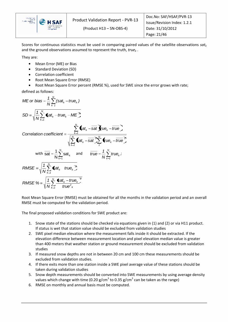
Scores for continuous statistics must be used in comparing paired values of the satellite observations satk and the ground observations assumed to represent the truth, truek .
They are:
Mean Error (ME) or Bias
Standard Deviation (SD)
Correlation coefficient
Root Mean Square Error (RMSE)
Root Mean Square Error percent (RMSE %), used for SWE since the error grows with rate;
defined as follows: N
1k
kk )true(satN
1biasorME
N
1k
2
kk MEtruesatN
1SD
N
1k
N
1
2
k
2
k
N
1k
kk
truetruesatsat
truetruesatsat
tcoefficiennCorrelatio
with N
1k
ksatN
1sat and
N
1k
ktrueN
1true ;
N
1k
2
kk truesatN
1RMSE
N
1k
2
k2
kk
true
truesat
N
1%RMSE
Root Mean Square Error (RMSE) must be obtained for all the months in the validation period and an overall RMSE must be computed for the validation period. The final proposed validation conditions for SWE product are:
1. Snow state of the stations should be checked via equations given in (1) and (2) or via H11 product. If status is wet that station value should be excluded from validation studies
2. SWE pixel median elevation where the measurement falls inside it should be extracted. If the elevation difference between measurement location and pixel elevation median value is greater than 400 meters that weather station or ground measurement should be excluded from validation studies
3. If measured snow depths are not in between 20 cm and 100 cm these measurements should be excluded from validation studies.
4. If there exits more than one station inside a SWE pixel average value of these stations should be taken during validation studies
5. Snow depth measurements should be converted into SWE measurements by using average density values which change with time (0.20 g/cm3 to 0.35 g/cm3 can be taken as the range)
6. RMSE on monthly and annual basis must be computed.
Product Validation Report - PVR-13
(Product H13 – SN-OBS-4)
Doc.No: SAF/HSAF/PVR-13
Issue/Revision Index: 1.2.1
Date: 31/10/2012
Page: 22/46
To complement the validation, 3 case studies for the reference season should be presented. For each case study quantitative analysis in the same manner like for the longer period (explained above) should be performed. Additionally, qualitative analysis by comparing pictures of H13 product with different satellite products (e.g. MODIS SWE products) should be performed. For each case study teams are welcome to introduce their own additional analysis or algorithms.
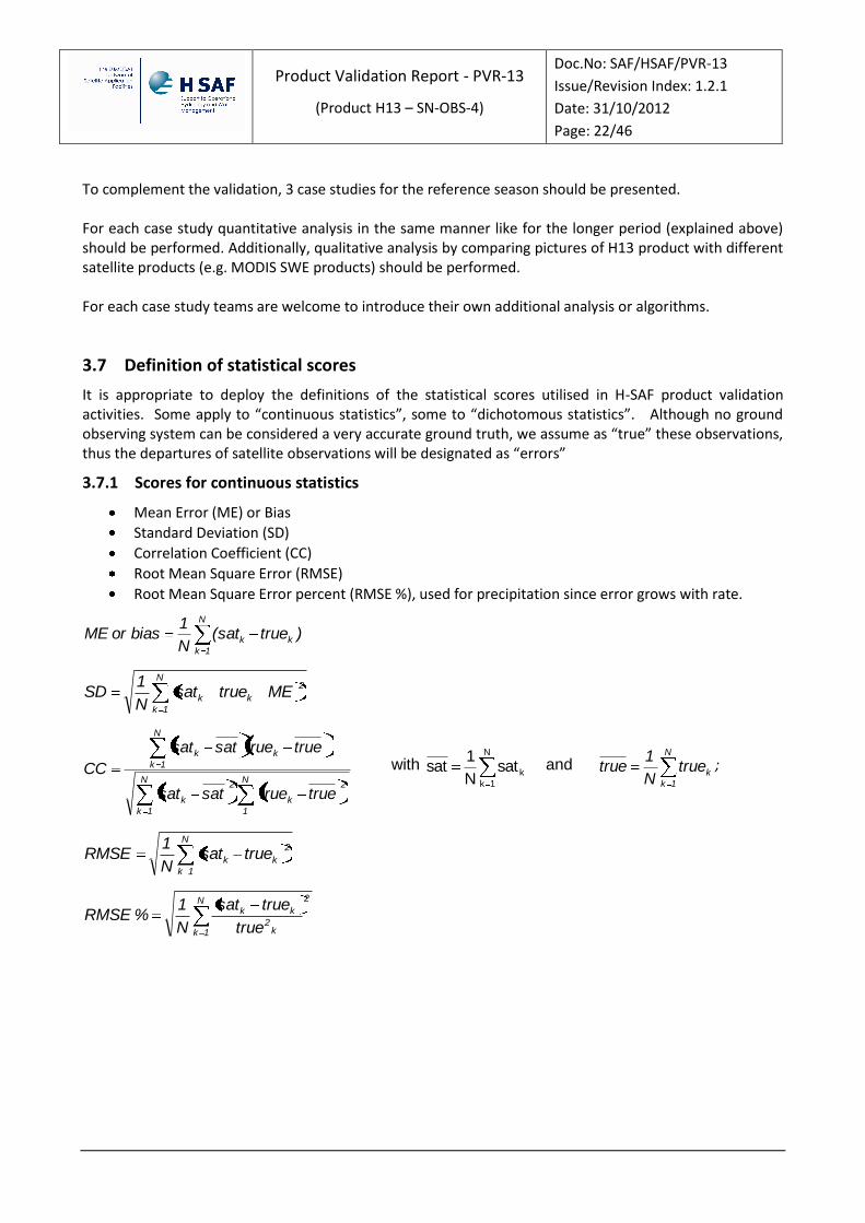
3.7 Definition of statistical scores
It is appropriate to deploy the definitions of the statistical scores utilised in H-SAF product validation activities. Some apply to “continuous statistics”, some to “dichotomous statistics”. Although no ground observing system can be considered a very accurate ground truth, we assume as “true” these observations, thus the departures of satellite observations will be designated as “errors”
3.7.1 Scores for continuous statistics
Mean Error (ME) or Bias
Standard Deviation (SD)
Correlation Coefficient (CC)
Root Mean Square Error (RMSE)
Root Mean Square Error percent (RMSE %), used for precipitation since error grows with rate.
N
1k
kk )true(satN
1biasorME
N
1k
2
kk MEtruesatN
1SD
N
1k
N
1
2
k
2
k
N
1k
kk
truetruesatsat
truetruesatsat
CC with N
1k
ksatN
1sat and
N
1k
ktrueN
1true ;
N
1k
2
kk truesatN
1RMSE
N
1k
2
k2
kk
true
truesat
N
1%RMSE
Product Validation Report - PVR-13
(Product H13 – SN-OBS-4)
Doc.No: SAF/HSAF/PVR-13
Issue/Revision Index: 1.2.1
Date: 31/10/2012
Page: 23/46
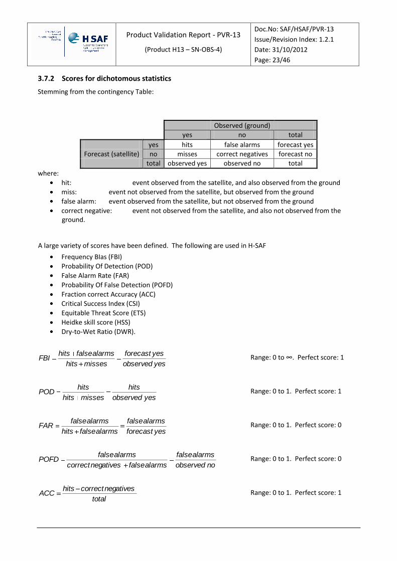
3.7.2 Scores for dichotomous statistics
Stemming from the contingency Table:
Observed (ground)
yes no total
yes hits false alarms forecast yes
Forecast (satellite) no misses correct negatives forecast no
total observed yes observed no total
where:
hit: event observed from the satellite, and also observed from the ground
miss: event not observed from the satellite, but observed from the ground
false alarm: event observed from the satellite, but not observed from the ground
correct negative: event not observed from the satellite, and also not observed from the ground.
A large variety of scores have been defined. The following are used in H-SAF
Frequency BIas (FBI)
Probability Of Detection (POD)
False Alarm Rate (FAR)
Probability Of False Detection (POFD)
Fraction correct Accuracy (ACC)
Critical Success Index (CSI)
Equitable Threat Score (ETS)
Heidke skill score (HSS)
Dry-to-Wet Ratio (DWR).
yesobserved
yesforecast
misseshits
alarmsfalsehitsFBI Range: 0 to ∞. Perfect score: 1
yesobserved
hits
misseshits
hitsPOD Range: 0 to 1. Perfect score: 1
yesforecast
alarmsfalse
alarmsfalsehits
alarmsfalseFAR Range: 0 to 1. Perfect score: 0
noobserved
alarmsfalse
alarmsfalsenegativescorrect
alarmsfalsePOFD Range: 0 to 1. Perfect score: 0
total
negativescorrecthitsACC Range: 0 to 1. Perfect score: 1

Product Validation Report - PVR-13
(Product H13 – SN-OBS-4)
Doc.No: SAF/HSAF/PVR-13
Issue/Revision Index: 1.2.1
Date: 31/10/2012
Page: 24/46
alarmfalsemisseshits
hitsCSI Range: 0 to 1. Perfect score: 1
random
random
hitsalarmfalsemisseshits
hitshitsETS with
total
yesforecastyesobservedhitsrandom
ETS ranges from -1/3 to 1. 0 indicates no skill. Perfect score: 1.
random
random
correct)pected(exN
correct)pected(exnegatives)correct(hitsHSS with
no)edno)(observ(forecastyes)astyes)(forec(observedN
1correct)pected(ex random
HSS
ranges from -1 to 1. 0 indicates no skill. Perfect score: 1.
yesobserved
no observed
misseshits
negative correctalarm falseDWR Range: 0 to ∞. Perfect score: n/a.
Product Validation Report - PVR-13
(Product H13 – SN-OBS-4)
Doc.No: SAF/HSAF/PVR-13
Issue/Revision Index: 1.2.1
Date: 31/10/2012
Page: 25/46
4 Ground data used for validation activities
4.1 Ground data in Finland (FMI)
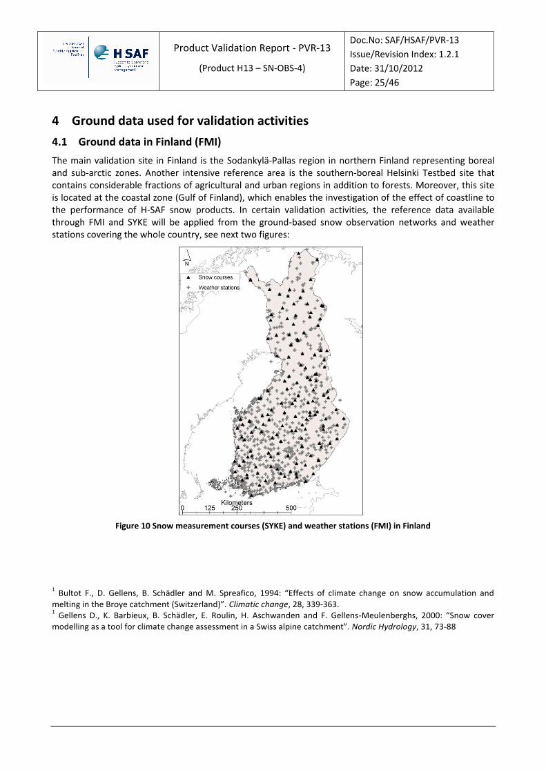
The main validation site in Finland is the Sodankylä-Pallas region in northern Finland representing boreal and sub-arctic zones. Another intensive reference area is the southern-boreal Helsinki Testbed site that contains considerable fractions of agricultural and urban regions in addition to forests. Moreover, this site is located at the coastal zone (Gulf of Finland), which enables the investigation of the effect of coastline to the performance of H-SAF snow products. In certain validation activities, the reference data available through FMI and SYKE will be applied from the ground-based snow observation networks and weather stations covering the whole country, see next two figures:
Figure 10 Snow measurement courses (SYKE) and weather stations (FMI) in Finland
1 Bultot F., D. Gellens, B. Schädler and M. Spreafico, 1994: “Effects of climate change on snow accumulation and
melting in the Broye catchment (Switzerland)”. Climatic change, 28, 339-363. 1 Gellens D., K. Barbieux, B. Schädler, E. Roulin, H. Aschwanden and F. Gellens-Meulenberghs, 2000: “Snow cover
modelling as a tool for climate change assessment in a Swiss alpine catchment”. Nordic Hydrology, 31, 73-88
Product Validation Report - PVR-13
(Product H13 – SN-OBS-4)
Doc.No: SAF/HSAF/PVR-13
Issue/Revision Index: 1.2.1
Date: 31/10/2012
Page: 26/46
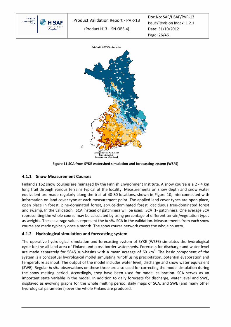
Figure 11 SCA from SYKE watershed simulation and forecasting system (WSFS)
4.1.1 Snow Measurement Courses
Finland's 162 snow courses are managed by the Finnish Environment Institute. A snow course is a 2 - 4 km long trail through various terrains typical of the locality. Measurements on snow depth and snow water equivalent are made regularly along the trail at 40-80 locations, shown in Figure 10, interconnected with information on land cover type at each measurement point. The applied land cover types are open place, open place in forest, pine-dominated forest, spruce-dominated forest, deciduous tree-dominated forest and swamp. In the validation, SCA instead of patchiness will be used: SCA=1- patchiness. One average SCA representing the whole course may be calculated by using percentage of different terrain/vegetation types as weights. These average values represent the in situ SCA in the validation. Measurements from each snow course are made typically once a month. The snow course network covers the whole country.
4.1.2 Hydrological simulation and forecasting system
The operative hydrological simulation and forecasting system of SYKE (WSFS) simulates the hydrological cycle for the all land area of Finland and cross border watersheds. Forecasts for discharge and water level are made separately for 5845 sub-basins with a mean acreage of 60 km2. The basic component of the system is a conceptual hydrological model simulating runoff using precipitation, potential evaporation and temperature as input. The output of the model includes water level, discharge and snow water equivalent (SWE). Regular in situ observations on these three are also used for correcting the model simulation during the snow melting period. Accordingly, they have been used for model calibration. SCA serves as an important state variable in the model. In addition to daily forecasts for discharge, water level and SWE, displayed as evolving graphs for the whole melting period, daily maps of SCA, and SWE (and many other hydrological parameters) over the whole Finland are produced.

Product Validation Report - PVR-13
(Product H13 – SN-OBS-4)
Doc.No: SAF/HSAF/PVR-13
Issue/Revision Index: 1.2.1
Date: 31/10/2012
Page: 27/46
4.1.3 The Sodankylä-Pallas validation region
The Sodankylä-Pallas site is a typical representative of Eurasian taiga belt characterized by a mosaic of sparse conifer-dominated forests and open/forested bogs. The landscape is generally relatively flat or gently rolling although small mountain regions (fjelds) are typical. The land use map of the region provided by SYKE is shown in next figure (land cover and forest characteristics with a spatial resolution of 25 m). The map shows the location of the site with intensive research stations at the town of Sodankylä and Pallas Mountain indicated.
Pallas
FMI-ARC at Sodankylä
100 km
Figure 12 Land cover map of the Sodankylä-Pallas site
Coniferous forests on mineral soil are depicted by dark green colour. Light green colour depicts sparse coniferous dominated forests (mainly on peat soil) and open bogs are depicted by grey. Open rock and barren areas (fjelds) are shown by brownish colours and open water by blue. Buildings and urban regions are depicted by red. The data sets available for the Sodankylä-Pallas region include the weather and atmospheric parameter monitoring data from the Finnish Meteorological Institute (FMI), land cover characteristics and hydrological monitoring and modelling data from the Finnish Environment Institute (SYKE), and selected data sets form other Finnish research institutes and universities. Intensive stations equipped with a large variety of atmospheric sampling, profiling and automatic surface parameter measurement systems are located near the town of Sodankylä (Arctic Research Centre of FMI with a permanent staff of around 30 persons), and at/in the vicinity of Pallas Mountain. Additional data sets are available from in situ and aerial monitoring campaigns, e.g. brightness temperature and reflectance data sets by Helsinki University of Technology (TKK).
4.2 Ground data in Turkey (ITU)
Modelling and algorithm developed for product generation imply calibration and validation activity as an integral part. The routine generation includes a certain amount of on-line re-calibration/validation to monitor product quality stability and continuously improve error structure characterisation. Snow cover mapping in mountainous areas is demanding due to the interfering topography and the heterogeneous ground properties.
Product Validation Report - PVR-13
(Product H13 – SN-OBS-4)
Doc.No: SAF/HSAF/PVR-13
Issue/Revision Index: 1.2.1
Date: 31/10/2012
Page: 28/46
Various types of observations from different institutions will be used as the auxiliary data for the preparation of data set to be used in cal/val process. For instance, State Hydraulic Works will be in charge of providing discharge and ground truth observations in the basins selected as test sites. Meteorological observations will be mainly provided by the currently operational sites in the basins and those planned to be deployed by TSMS in a near future. In addition, other observation sites located in the vicinity of the basins will be used whenever needed. The snow product calibration and validation in Turkey will be performed using independent snow course measurements, and higher resolution satellite images.
It is very difficult and expensive to collect hydro-meteorological data at higher altitudes especially in extreme climatic conditions. However, it is essential to characterize climate conditions over the rough topography of the remote mountainous catchments in Eastern Turkey where large portion of the water to the large dams originates from snowmelt during spring and early summer months.
There are:
5 Automated Weather Operating Stations (AWOS)
2 Synoptic Stations
5 Climatologic Stations
3 Automated Stream Gauging Stations
5 Snow Courses
in and around the basin selected as the medium scale test site.
Automated Weather Operating Stations (AWOS) collect 2-hour data (temperature, precipitation, radiation, albedo, wind speed and direction, relative humidity, air pressure, soil temperature, snow depth, snow density, snow lysimeter) that are in real-time format. Synoptic stations collect 1 to 3 hour data (temperature, precipitation, radiation, wind speed and direction, relative humidity, air pressure, evaporation, soil temperature, snow depth) that are received with 1-day delay. Climatologic stations collect data hourly (temperature, air pressure, wind speed and direction) and three times a day (relative humidity, evaporation and precipitation) that are received with 1-month delay. Stream Gauging Stations (SGS) collect 15 to 60 minute data (stream depth converted into discharge) that are in real-time format. Finally, manual snow courses are conducted every two to three weeks during the period with snow cover and data can be transferred with 1-week delay.
Hydro-meteorological data are provided from the stations operating at various locations and altitudes in Upper Euphrates Basin. But since ground based observations can only represent a small part of the region of interest, spatially and temporally distributed snow data are needed. Distribution of the ground data using a proper interpolation technique suffer of the limitations of the interpolation methods in predicting snow parameters for rough terrain. Therefore higher spatial resolution data (e.g. Landsat, Quickbird, Ikonos images) will be also used for validation of the snow recognition and effective snow cover products. The cloud problem will be encountered by performing monitoring during melting period.
For snow water equivalent product, besides ground observations, snow water equivalent values obtained as the output of outputs from snowpack surface energy balance model will be used. Net energy fluxes are calculated for each pixel using the snowpack surface energy balance model that operates at a 1-km spatial resolution. The output from the snow hydrology model is snow depth, density, grain size, and temperature. These parameters are determined for each pixel on an hourly basis. It is believed that comparing the SWE retrieval with modelled SWE values is important from the hydrological point of view. Considering that all the H-SAF products will be used in hydrological impact studies, so in this case study it is tried to compare the use of HSAF SWE product with the modelled SWE obtained from hydrological modelling. SWE value is most of the time an internal parameter to be estimated in hydrological modelling. It is also possible to assimilate the space borne SWE products during the

Product Validation Report - PVR-13
(Product H13 – SN-OBS-4)
Doc.No: SAF/HSAF/PVR-13
Issue/Revision Index: 1.2.1
Date: 31/10/2012
Page: 29/46
modelling in order to improve the runoff estimates. In the present case study the coarse resolution of HSAF SWE product was improved by applying HSAF fractional snow product (H12) as a mask. In Table 3 the measured SD values (the last column of the table) were also used in the comparison. The dates Feb 9, 2010 and March 12, 2011 were selected because on these days maximum SWE was observed in the basin. The mean snow depth obtained from the ground observations was 42.5 cm on March 12, 2011. The measured SWE was calculated as multiplying the SD with a mean density value. So 106 mm is the measured SWE for March 12, 2011. 75 mm was obtained from hydrological modelling and 105 mm was obtained from HSAF SWE product. This result indicates the performance of the HSAF SWE product compared to modelled SWE obtained from hydrological modelling. This case study analysis will be deeper discussed in the next version of PVR-13.
Product Validation Report - PVR-13
(Product H13 – SN-OBS-4)
Doc.No: SAF/HSAF/PVR-13
Issue/Revision Index: 1.2.1
Date: 31/10/2012
Page: 30/46
5 Validation results: case study analysis
5.1 Case Studies in Turkey
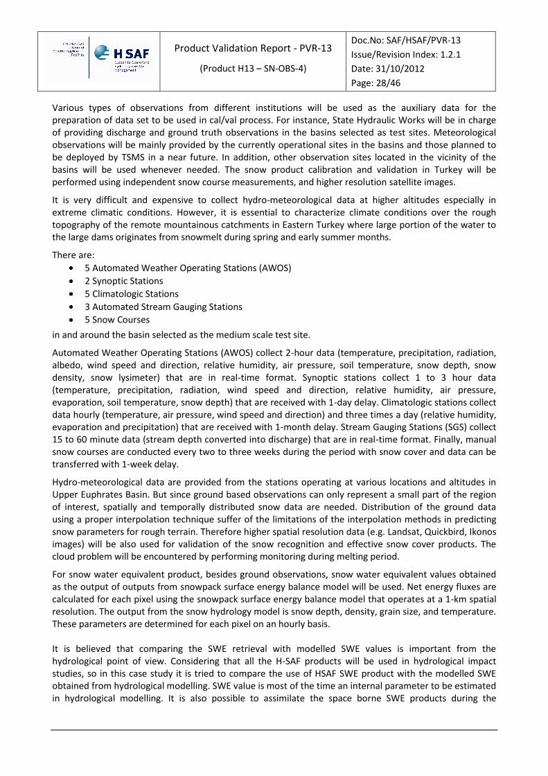
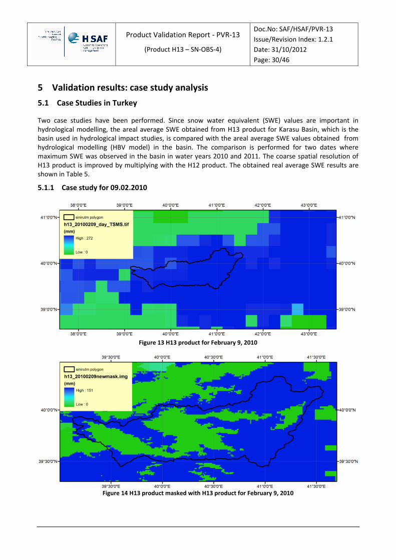
Two case studies have been performed. Since snow water equivalent (SWE) values are important in hydrological modelling, the areal average SWE obtained from H13 product for Karasu Basin, which is the basin used in hydrological impact studies, is compared with the areal average SWE values obtained from hydrological modelling (HBV model) in the basin. The comparison is performed for two dates where maximum SWE was observed in the basin in water years 2010 and 2011. The coarse spatial resolution of H13 product is improved by multiplying with the H12 product. The obtained real average SWE results are shown in Table 5.
5.1.1 Case study for 09.02.2010
Figure 13 H13 product for February 9, 2010
Figure 14 H13 product masked with H13 product for February 9, 2010
Product Validation Report - PVR-13
(Product H13 – SN-OBS-4)
Doc.No: SAF/HSAF/PVR-13
Issue/Revision Index: 1.2.1
Date: 31/10/2012
Page: 31/46
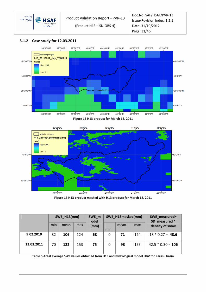
5.1.2 Case study for 12.03.2011
Figure 15 H13 product for March 12, 2011
Figure 16 H13 product masked with H13 product for March 12, 2011
SWE_H13(mm) SWE_m
odel (mm)
SWE_H13masked(mm) SWE_measured= SD_measured * density of snow min mean max
min mean max
9.02.2010 82 106 124 68 0 71 124 18 * 0.27 = 48.6
12.03.2011 70 122 153 75 0 98 153 42.5 * 0.30 = 106
Table 5 Areal average SWE values obtained from H13 and hydrological model HBV for Karasu basin

Product Validation Report - PVR-13
(Product H13 – SN-OBS-4)
Doc.No: SAF/HSAF/PVR-13
Issue/Revision Index: 1.2.1
Date: 31/10/2012
Page: 32/46
In Table 5 the measured SD values (the last column of the table) were also used in the comparison. The dates Feb 9, 2010 and March 12, 2011 were selected due to the maximum SWE observed in the basin. The mean snow depth obtained from the ground observations was 42.5 cm on March 12, 2011. The measured SWE was calculated as multiplying the SD with a mean density value, where 106 mm is the measured SWE for March 12, 2011. While 75 mm was obtained from hydrological modeling and 98 mm was obtained from HSAF SWE product. This result indicates the performance of the HSAF SWE product compared to modeled SWE obtained from hydrological modeling.
Product Validation Report - PVR-13
(Product H13 – SN-OBS-4)
Doc.No: SAF/HSAF/PVR-13
Issue/Revision Index: 1.2.1
Date: 31/10/2012
Page: 33/46
6 Validation results: long statistic analysis
6.1 Introduction
In this Chapter the validation results of the H13 large statistics analysis are reported for the period (10.2009 – 09.2012). The validation has been performed on the product release currently in force at the time of writing.
Finland and Turkey contributed to this Chapter by providing the overall accuracy on national territory. The ground data used for the validation have been described in Chapter 4.
To assess the degree of compliance of the product with product requirements (see [RD1]), all the PPVG members provided the long statistic results following the validation methodology reported in Chapter 3. For product H13 the product requirements are recorded in Table 6.
score threshold target optimal
flat 40mm 20mm 10mm
mountain 45mm 25mm 15mm Table 6 Accuracy requirements for product PR-OBS-13 [RMSE]
This implies that the main score to be evaluated has been the Root Mean Square error (mm). These scores have been defined in section 3.7.
The long statistic results obtained in Finland and Turkey will be showed in the next sections.
6.2 Validation exercises in Turkey
The validation of SWE from microwave imagery from SSMI/S (merged H13 product) is performed against synoptic, climate, and automated weather observation stations. The snow depth measurements obtained from the ground stations are used (Figure 1). The in-situ data falling in the mountainous mask are included in the validation analysis. The validation dataset covers the period of January 2010-April 2010, January 2011-March 2011 and January 2012-March 2012 with 1955 in-situ measurements from 31 stations.
6.3 Validation with synoptic weather station data
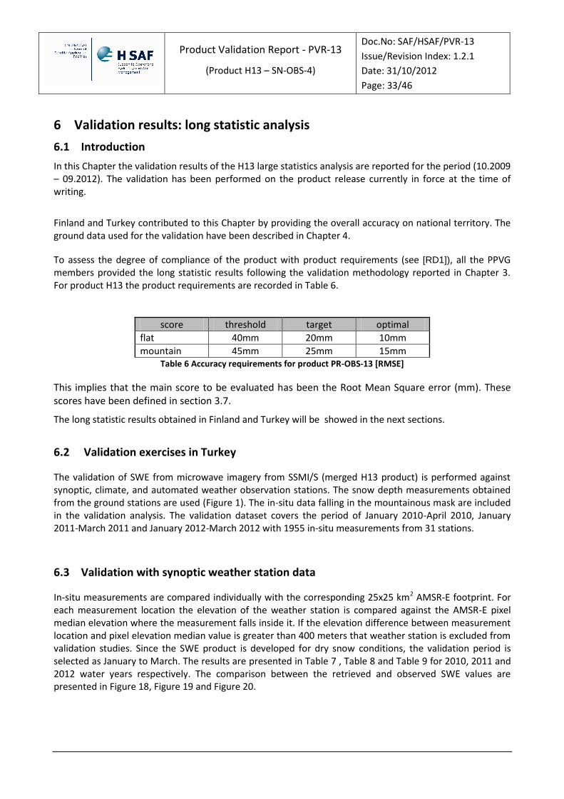
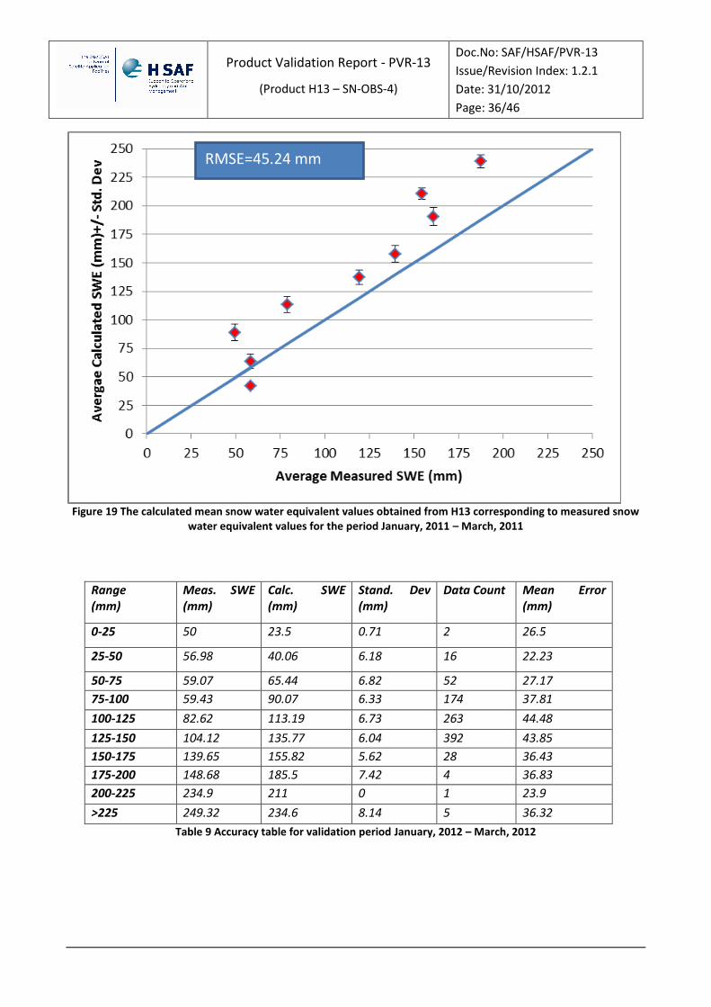
In-situ measurements are compared individually with the corresponding 25x25 km2 AMSR-E footprint. For each measurement location the elevation of the weather station is compared against the AMSR-E pixel median elevation where the measurement falls inside it. If the elevation difference between measurement location and pixel elevation median value is greater than 400 meters that weather station is excluded from validation studies. Since the SWE product is developed for dry snow conditions, the validation period is selected as January to March. The results are presented in Table 7 , Table 8 and Table 9 for 2010, 2011 and 2012 water years respectively. The comparison between the retrieved and observed SWE values are presented in Figure 18, Figure 19 and Figure 20.
Product Validation Report - PVR-13
(Product H13 – SN-OBS-4)
Doc.No: SAF/HSAF/PVR-13
Issue/Revision Index: 1.2.1
Date: 31/10/2012
Page: 34/46
Figure 17 TSMS synoptic, climate and AWOS stations reporting snow depths
Range (mm)
Meas. SWE (mm)
Calc. SWE (mm)
Stand. Dev (mm)
Data Count Mean Error (mm)
0-50 50.70 44.00 3.16 4 23.20
50-75 48.68 63.13 7.63 24 25.89
75-100 57.79 89.81 6.52 108 38.45
100-125 77.28 111.72 6.45 141 42.95
125-150 94.10 133.89 4.46 19 44.16
150-175 NA NA NA 0 NA
175-200 165.00 181.00 0.00 1 16.0
200-225 NA NA NA 0 NA
Table 7 Results for validation period January, 2010 – March, 2010

Product Validation Report - PVR-13
(Product H13 – SN-OBS-4)
Doc.No: SAF/HSAF/PVR-13
Issue/Revision Index: 1.2.1
Date: 31/10/2012
Page: 35/46
Figure 18 The calculated mean snow water equivalent obtained from H13 corresponding to measured snow water
equivalent values for the period January, 2010 – March, 2010
Range (mm)
Meas. SWE (mm)
Calc. SWE (mm)
Stand. Dev (mm)
Data Count Mean Error (mm)
0-50 58.4 41.75 6.26 48 22.83
50-75 58.18 63.33 7.20 86 25.93
75-100 49.40 88.89 7.01 175 42.63
100-125 78.85 113.45 6.41 202 45.40
125-150 119.30 137.32 7.25 136 42.80
150-175 139.35 157.66 7.73 29 36.51
175-200 160.80 190.60 5.13 5 32.2
200-225 154.28 210.75 5.44 4 56.48
>225 187.38 239 6.28 5 51.62
Table 8 Accuracy table for validation period January, 2011 – March, 2011
RMSE=44.61 mm
Product Validation Report - PVR-13
(Product H13 – SN-OBS-4)
Doc.No: SAF/HSAF/PVR-13
Issue/Revision Index: 1.2.1
Date: 31/10/2012
Page: 36/46
Figure 19 The calculated mean snow water equivalent values obtained from H13 corresponding to measured snow
water equivalent values for the period January, 2011 – March, 2011
Range (mm)
Meas. SWE (mm)
Calc. SWE (mm)
Stand. Dev (mm)
Data Count Mean Error (mm)
0-25 50 23.5 0.71 2 26.5
25-50 56.98 40.06 6.18 16 22.23
50-75 59.07 65.44 6.82 52 27.17
75-100 59.43 90.07 6.33 174 37.81
100-125 82.62 113.19 6.73 263 44.48
125-150 104.12 135.77 6.04 392 43.85
150-175 139.65 155.82 5.62 28 36.43
175-200 148.68 185.5 7.42 4 36.83
200-225 234.9 211 0 1 23.9
>225 249.32 234.6 8.14 5 36.32
Table 9 Accuracy table for validation period January, 2012 – March, 2012
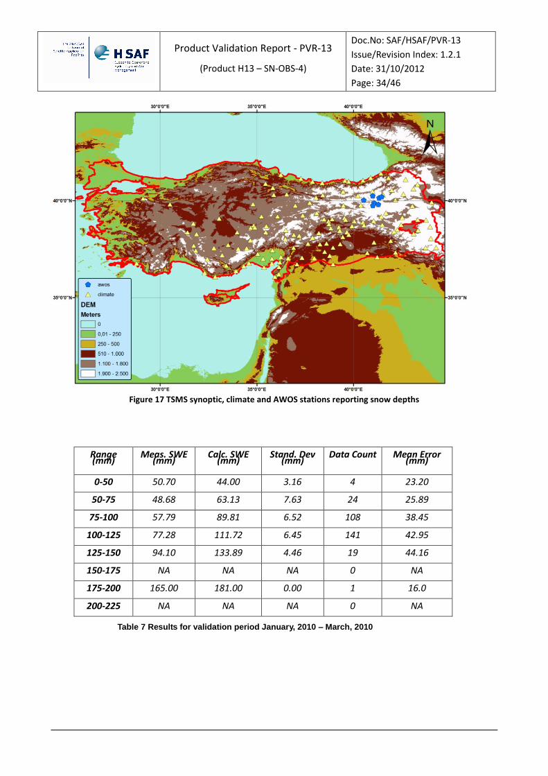
RMSE=45.24 mm

Product Validation Report - PVR-13
(Product H13 – SN-OBS-4)
Doc.No: SAF/HSAF/PVR-13
Issue/Revision Index: 1.2.1
Date: 31/10/2012
Page: 37/46
Figure 20 The calculated mean snow water equivalent values obtained from H13 corresponding to measured snow water equivalent values for the period January, 2012 – March, 2012 Topography greatly reduces the accuracy of any space borne radiometer-based SWE retrievals for mountains regions. Microwave instruments have capability to penetrate into snow pack having depth up to 80 cm (SWE=150 mm) and for snow depths less than 20 cm (SWE=50 mm) depth ground surface contribution dominates the measured brightness temperature (Ulaby et al., 1981). In Table 7, Table 8 and Table 9 the standard deviations of the calculated SWE values should be taken into consideration during evaluation of the validation results. Referring to Table 7, for SWE range 75-100 mm and the measured average is 57.79 mm.
6.4 Validation results in Finland
Due to break up of AMSR-E instrument the processing chain of H-13 product has been converted to new baseline using SSMI/S radiometer data. The H-13 processor with new satellite sensor baseline was applied for years from 2006 to 2010 (5 years). Finland does not have mountainous regions so all the data points within Finland are produced by flat lands algorithm. Since the reference data is available only once a month the H-13 product is weekly averaged to better correspond the reference data. Reference Data For flat lands the algorithm assimilates snow depth observations from weather stations. Thus special care is taken to ensure that reference data is independent of assimilated snow depth observations. Finnish Environment Institute SYKE collects snow water equivalent data from snow courses once a month. Multiple sampling with varying land use characteristics ensures that data is a good representative of the local SWE. For example, for year 2010 there were 153 snow courses reporting SWE. Results In Figure 21 H-13 validation results are presented in Finland from 2006 to 2010.
RMSE=45.54 mm

Product Validation Report - PVR-13
(Product H13 – SN-OBS-4)
Doc.No: SAF/HSAF/PVR-13
Issue/Revision Index: 1.2.1
Date: 31/10/2012
Page: 38/46
Figure 21 validation results in Finland
Parameters calculated are bias 4.4 mm, rms (without bias correction) 35.87 mm, rms (with bias correction) 35.60 mm, correlation coefficient 0.71 and number of samples 2407.
6.5 Some conclusions
The overall accuracy has been evaluated for the period October, 2010 – March, 2012 in Turkey. The averaged overall accuracy obtained is equal to 45.13 mm. The overall accuracy for flat lands in Finland has been calculated for the period 2006-2010 and the averaged overall accuracy is equal to 35.735 mm. As shown in the following table the statistical scores obtained by the validation of H13 in SPVG are really close to the thresholds stated in the Product requirements (see [RD1]) for Turkey, and between threshold and target for Finland.

Product Validation Report - PVR-13
(Product H13 – SN-OBS-4)
Doc.No: SAF/HSAF/PVR-13
Issue/Revision Index: 1.2.1
Date: 31/10/2012
Page: 39/46
Between target and optimal
Between threshold and target
Threshold exceeded by < 50 %
Threshold exceeded by ≥ 50 %
Table 10 Simplified compliance analysis for product H13
Product requirements H13
area threshold target optimal total
flat 40mm 20mm 10mm 36mm
mountain 45mm 25mm 15mm 45mm Table 11 H-SAF Accuracy requirements for H13 [RMSE]
Some general consideration when comparing the results from the validation activity with the stated product requirements:
a. Product requirements - There are reasons to believe that the current set of H-SAF Product requirements have been overstated.
b. The results obtained by the current validation procedure represent the convolution of at least three factors: the satellite product accuracy, the accuracy of the ground data used and the limitations of the comparison methodology (e.g., errors of space and time co-location, representativeness changing with scale, etc.). Therefore, the results currently found are by far pessimistic in respect of what is the real product performance.
c. Largest RMSE is observed for month February. This is due to starting of melting of snow at the stations located at altitude lower than 1000 m in February. The mean altitude of the synoptic and climate stations is 1260 m where the mean altitude of automatic weather observation stations is 2673 m.
The H-13 product estimates SWE very well up till ground truth snow measurement values of 150 mm. There is a small positive bias. Once ground truth values are over 150 mm the H-13 underestimates SWE visibly. This is due to the saturation of brightness temperature signatures in thick snowpacks. On the other hand, algorithms relying spaceborne data in general saturate with lower values of SWE than H-13 algorithm. If ground truth data is investigated most of the actual SWE values are in the region < 150 mm and larger values are rare. The rms value of 35.87 mm (without bias correction) shows a good agreement of H-13 estimates with ground reference data.

Product Validation Report - PVR-13
(Product H13 – SN-OBS-4)
Doc.No: SAF/HSAF/PVR-13
Issue/Revision Index: 1.2.1
Date: 31/10/2012
Page: 40/46
7 Conclusions
7.1 Summary conclusions on product validation
The number of ground data is few. Also, the ground measurements are not evenly distributed within the resolution elements, so the whole area of individual footprint is not examined properly. The coarse spatial resolution and the penetration characteristics of the SSMI/S instrument for shallow and deep snow may lead under and over estimation in the SWE retrieval. The major trend is over estimation of H13 product compared to ground observations, but the low standard deviation in the average calculated SWE values for the given ranges indicate the consistency of the product for different ranges. The overall RMSE for January 2010-April 2010, January 2011-April 2011 and January 2012-April 2012 is 44.61 mm, 45.24 mm and 45.54 mm, respectively. The results indicate that the threshold product requirement which is 45 mm for the mountainous areas is already satisfied.
The use of SWE from H13 product in hydrological studies is important. Neither ground observation nor the satellite products can be sufficient in hydrological modelling. Both of them must be used in the modelling. The use of assimilated SCA or SWE in operational forecasting will improve the results of hydrograph predictions. Through the case studies applying the H12 snow product as a mask in order to increase the spatial resolution of the H13 product improve the SWE distribution in the basin. The areal average SWE values from the product and the model results get closer with the mask application. The difference in the areal average SWE value obtained from H13 and the model results for February 9, 2010 is less. Due to high cloud coverage on that day H12 product for February 20, 2010, which is less cloudy, is applied as the mask. The snow may melt during this 11 days delay, but still the values are comparative with the model results considering the fact that the model underestimates SWE during modelling due to several limitations in the model. The snow depths measured at a ground station in the basin are also used to estimate the SWE value at a point on the corresponding day. For February the measured SWE value is less than the estimated SWE value from H13 product and hydrological model. For March the measured SWE value is close to the SWE value estimated from H13 product after the mask is applied, where the SWE obtained from the model is low compared to the measured and estimated SWE values.
As Fig. 1 suggests, the H-13 product estimates SWE very well up till ground truth snow measurement values of 150 mm. There is a small positive bias. Once ground truth values are over 150 mm the H-13 underestimates SWE visibly. This is due to the saturation of brightness temperature signatures in thick snowpacks. On the other hand, algorithms relying spaceborne data in general saturate with lower values of SWE than H-13 algorithm. If ground truth data is investigated most of the actual SWE values are in the region < 150 mm and larger values are rare. The rms value of 35.87 mm (without bias correction) shows a good agreement of H-13 estimates with ground reference data. The current implementation of H13 SWE algorithm for flat lands meets the product requirements defined in PRD if unbiased RMSE is considered. Even using biased RMSE the results are very close to the requirements. One can think bias as deterministic component of the error and the rest as a random component. The analysis shows that the algorithm performs worst during melt period in springtime. In one part this is due to the inherit properties of radiometry but especially the dry snow detection can be improved. During CDOP-2 algorithm development in this respect is foreseen.

Product Validation Report - PVR-13
(Product H13 – SN-OBS-4)
Doc.No: SAF/HSAF/PVR-13
Issue/Revision Index: 1.2.1
Date: 31/10/2012
Page: 41/46
8 Reference documents
[RD1] Product Requirement Document, SAF/HSAF/PRD/1.3
Product Validation Report - PVR-13
(Product H13 – SN-OBS-4)
Doc.No: SAF/HSAF/PVR-13
Issue/Revision Index: 1.2.1
Date: 31/10/2012
Page: 42/46
Annex 1. Validation methodology for H13 – Snow water equivalent
Zuhal Akyurek, [email protected], Matias Takala, [email protected]
This document describes the methodology applied for validating H-SAF snow product H13 – Snow Water Equivalent by MW radiometry. Validation procedure To properly validate H13 product, the following steps have to be taken:
1. Observation data containing snow depth, or SWE measurements have to be gathered. If only snow depth is gathered average snow density values ranging in between 0.20 g/cm3 to 0.35 g/cm3 can be used to calculate SWE. This range is valid for the period of January to March.
2. In flatlands to properly validate H13 the ground truth data should not be pointwise in nature (measurement in single location) but obtained from a path of observations.
3. Satellite product needs to be acquired. 4. Both observation and satellite data series need to be checked for consistency. 5. Comparison between the observation data and the product has to be performed. 6. Results of the comparison need to be presented.
1. Observation data From the data collected by ground network, a subset containing snow cover depth for the reference season (1.10.2009 – 31.09.2010) is extracted and a local database is created. The data is stored in plain text. Each file contains the data from all reporting stations for one day of the reference season. For each station the following columns (separated by whitespace) are assigned:
date and time of measurement,
number and name of the station as well as it's coordinates (Latitude(degrees), Longitude(degrees) and height (m) asl.,
a flag indicating whether the station is located in mountainous or flat/forested area. The masking is performed by applying the mountain mask. The file “mountainmask_swe.h5” is in TSMS ftp site at /OUT/h13/mountainmask address: ftp://hsaf.meteoroloji.gov.tr username: snowtur password: rs37kar
snow cover depth (in cm) or snow water equivalent (mm) . 2. Satellite product H-SAF H13product is available at the FMI ftp server, ftp://ftp.fmi.fi. An ftp client (e.g. FileZilla, WinSCP) is required to log in and retrieve the product, which is stored in the binary HDF5 files. 3. Data consistency check To guarantee high quality of the validation it is advised to check if both the observation data and the satellite product are available for all days of the reference season. 4. Comparison between the observation data and the product

Product Validation Report - PVR-13
(Product H13 – SN-OBS-4)
Doc.No: SAF/HSAF/PVR-13
Issue/Revision Index: 1.2.1
Date: 31/10/2012
Page: 43/46
Comparison for Flat/Forest Areas: Ground truth data and SWE estimate for Flat/Forest areas can be compared by selecting the ground truth value and the SWE value in the corresponding pixel. It should be noted that proper validation accuracy is obtained using SWE path observations. If pointwise ground truth data is used the accuracy is lower. Since H13 for Flat/Forest areas is an assimilation of weather station observations and satellite data care must be taken that the reference data is independent from the weather station data used in assimilation. Spaceborne SWE estimates can be reliably given only when snow is dry. The algorithm to detect dry snow is the same as for Mountainous areas (see next chapter). If the snow is dry the given SWE estimate is a statistically weighed combination of interpolated weather station SWE field and spaceborne SWE estimate. If the snow is wet only interpolated estimate is given. Thus any SWE value in the validation range from 20 cm to 100 cm can be used. To harmonize the validation analysis together with the Mountainous areas the results from product H11 can be used. The statistical figures to be computed in Flat/Forest areas are:
Mean Error (ME) or Bias
Standard Deviation (SD)
Correlation coefficient
Root Mean Square Error (RMSE)
Root Mean Square Error percent (RMSE %). For equations please see next chapter. The final proposed validation conditions for SWE product in flat lands are: 1. No additional separation between dry/wet snow needs to be done. To harmonize the validation
procedure with Mountainous areas one can use product H11. 2. Values from Mountainous areas are discarded. 3. If measured snow depths are not in between 20 cm and 100 cm these measurements should be
excluded from validation studies. 4. If there exits more than one station inside a SWE pixel average value of these stations should be taken
during validation studies 5. Snow depth measurements should be converted into SWE measurements by using average density
values which change with time (0.20 g/cm3 to 0.35 g/cm3 can be taken as the range). 6. RMSE on monthly and annual basis must be computed. Comparison for Mountainous areas: In-situ measurements can be compared individually with the corresponding 25x25 km2 AMSR-E footprint. For each measurement location the elevation of the weather station or ground measurement should be compared against the AMSR-E pixel median elevation where the measurement falls inside it. If the elevation difference between measurement location and pixel elevation median value is greater than 400 meters that weather station or ground measurement should be excluded from validation studies. The specified 400 meters threshold value can change locally and this value should be studied for validation area under consideration. It should be kept in mind that SWE product is developed for dry snow conditions. Therefore for any pixel, if snow status has been detected as wet, no SWE calculation was done and SWE value was set as 0.0 mm. Hall et al. (2002) describe a simple algorithm to detect snow status. First snow depth (SD) is determined by:

Product Validation Report - PVR-13
(Product H13 – SN-OBS-4)
Doc.No: SAF/HSAF/PVR-13
Issue/Revision Index: 1.2.1
Date: 31/10/2012
Page: 44/46
SD=15.6(Tb18.7h-Tb36.5h) (1)
where Tb is brightness temperature and subindices denote the channels. If the conditions in equation (2) are met the data is classified as dry snow.
SD>80 and Tb36.5v <250K and Tb36.5h <240K (2) Snow status product H11 can also be checked for the snow state of pixel in which validation measurement exists. If the snow state of station is stated as wet then that station should be excluded from validation studies. Developed algorithm for SWE is valid for snow depths in between 20 cm and 100 cm. Snow depths out of this range cannot be modeled because of capabilities of the sensor. Thus, during validation studies measured snow depths out of this range should be neglected. If there exists only snow depth measurements, these values should be multiplied with average snow densities that range in between 0.25 g/cm3 to 0.30 g/cm3 in order to obtain SWE values.
Scores for continuous statistics must be used in comparing paired values of the satellite observations satk and the ground observations assumed to represent the truth, truek .
They are:
Mean Error (ME) or Bias
Standard Deviation (SD)
Correlation coefficient
Root Mean Square Error (RMSE)
Root Mean Square Error percent (RMSE %), used for SWE since the error grows with rate;
defined as follows: N
1k
kk )true(satN
1biasorME
N
1k
2
kk MEtruesatN
1SD
N
1k
N
1
2
k
2
k
N
1k
kk
truetruesatsat
truetruesatsat
tcoefficiennCorrelatio
with N
1k
ksatN
1sat and
N
1k
ktrueN
1true ;
N
1k
2
kk truesatN
1RMSE

Product Validation Report - PVR-13
(Product H13 – SN-OBS-4)
Doc.No: SAF/HSAF/PVR-13
Issue/Revision Index: 1.2.1
Date: 31/10/2012
Page: 45/46
N
1k
2
k2
kk
true
truesat
N
1%RMSE
Root Mean Square Error (RMSE) must be obtained for all the months in the validation period and an overall RMSE must be computed for the validation period. The final proposed validation conditions for SWE product are: 1. Snow state of the stations should be checked via equations given in (1) and (2) or via H11 product. If
status is wet that station value should be excluded from validation studies 2. SWE pixel median elevation where the measurement falls inside it should be extracted. If the elevation
difference between measurement location and pixel elevation median value is greater than 400 meters that weather station or ground measurement should be excluded from validation studies
3. If measured snow depths are not in between 20 cm and 100 cm these measurements should be excluded from validation studies.
4. If there exits more than one station inside a SWE pixel average value of these stations should be taken during validation studies
5. Snow depth measurements should be converted into SWE measurements by using average density values which change with time (0.20 g/cm3 to 0.35 g/cm3 can be taken as the range)
6. RMSE on monthly and annual basis must be computed. To complement the validation, 3 case studies for the reference season should be presented. For each case study quantitative analysis in the same manner like for the longer period (explained above) should be performed. Additionally, qualitative analysis by comparing pictures of H13 product with different satellite products (e.g. MODIS SWE products) should be performed. For each case study teams are welcome to introduce their own additional analysis or algorithms. References:
1. Hall, D.K., Kelly, R.E.J, Riggs, G.A, Chang, A.T.C, and Foster, J.L. 2002, Assessment of the relative
accuracy of hemispheric-scale snow-cover maps., Annals of Glaciology, 34:24–30.
2. Pulliainen, J. 2006. Mapping of snow water equivalent and snow depth in boreal and sub-arctic zones
by assimilating space-borne microwave radiometer data and ground-based observations. Remote
Sensing of Environment, 101, 257-269.
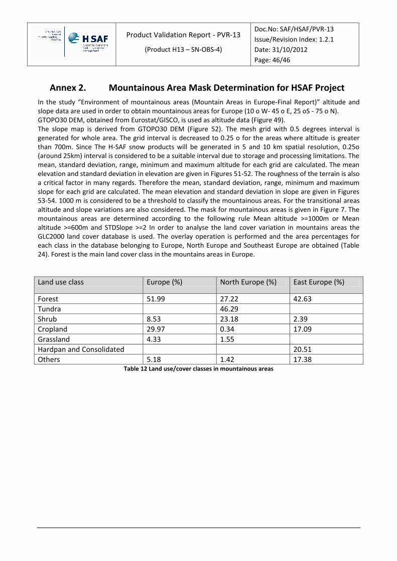
Product Validation Report - PVR-13
(Product H13 – SN-OBS-4)
Doc.No: SAF/HSAF/PVR-13
Issue/Revision Index: 1.2.1
Date: 31/10/2012
Page: 46/46
Annex 2. Mountainous Area Mask Determination for HSAF Project
In the study “Environment of mountainous areas (Mountain Areas in Europe-Final Report)” altitude and slope data are used in order to obtain mountainous areas for Europe (10 o W- 45 o E, 25 oS - 75 o N). GTOPO30 DEM, obtained from Eurostat/GISCO, is used as altitude data (Figure 49). The slope map is derived from GTOPO30 DEM (Figure 52). The mesh grid with 0.5 degrees interval is generated for whole area. The grid interval is decreased to 0.25 o for the areas where altitude is greater than 700m. Since The H-SAF snow products will be generated in 5 and 10 km spatial resolution, 0.25o (around 25km) interval is considered to be a suitable interval due to storage and processing limitations. The mean, standard deviation, range, minimum and maximum altitude for each grid are calculated. The mean elevation and standard deviation in elevation are given in Figures 51-52. The roughness of the terrain is also a critical factor in many regards. Therefore the mean, standard deviation, range, minimum and maximum slope for each grid are calculated. The mean elevation and standard deviation in slope are given in Figures 53-54. 1000 m is considered to be a threshold to classify the mountainous areas. For the transitional areas altitude and slope variations are also considered. The mask for mountainous areas is given in Figure 7. The mountainous areas are determined according to the following rule Mean altitude >=1000m or Mean altitude >=600m and STDSlope >=2 In order to analyse the land cover variation in mountains areas the GLC2000 land cover database is used. The overlay operation is performed and the area percentages for each class in the database belonging to Europe, North Europe and Southeast Europe are obtained (Table 24). Forest is the main land cover class in the mountains areas in Europe.
Land use class Europe (%) North Europe (%) East Europe (%)
Forest 51.99 27.22 42.63
Tundra 46.29
Shrub 8.53 23.18 2.39
Cropland 29.97 0.34 17.09
Grassland 4.33 1.55
Hardpan and Consolidated 20.51
Others 5.18 1.42 17.38 Table 12 Land use/cover classes in mountainous areas