production optimization and simulation of …ethesis.nitrkl.ac.in/3023/1/uttam_ghorai.pdf · table...
TRANSCRIPT

PRODUCTION OPTIMIZATION AND
SIMULATION OF LARGE OPEN CAST MINES
UTTAM GHORAI

ii
PRODUCTION OPTIMIZATION AND
SIMULATION OF LARGE OPEN CAST MINES
Thesis submitted to the
National Institute of Technology, Rourkela
For award of the Degree
of
Master of Technology (by Research)
by
Uttam Ghorai
Under the guidance of
Dr. B. K. Pal
DEPARTMENT OF MINING ENGINEERING
NATIONAL INSTITUTE OF TECHNOLOGY, ROURKELA –8.
APRIL 2011
iii
CERTIFICATE
This is to certify that the thesis entitled “PRODUCTION OPTIMIZATION AND
SIMULATION OF OPEN CAST MINES” Submitted by Uttam Ghorai to National
Institute of Technology, Rourkela, is record of bona fide research work under our supervision
and we consider it worthy of consideration for the award of the degree of Master of Technology
(by Research) of the Institute.
(Dr. B. K. Pal)
Professor and Supervisor
Department of Mining Engineering
NIT, Rourkela – 8.

iv
ACKNOWLEDGEMENT
The writing of the thesis has been one of the most significant academic challenges to me I have
ever faced. During this academic carrier I have the following people who were ultimate
supportive and helpful. Without their constant support I probably cannot reach the goal. I convey
my heartiest gratitude to all of them.
• I express my cordial sense of gratitude and thanks to Dr. B. K. Pal for his invaluable time,
guidance and help in spite of his very busy schedule. I have working under him for past three
years. He helped me all the way to complete the thesis.
• I would like to thank all faculty members and staffs of Department of Mining Engineering
who help me a lot.
• I would also like to thank Dr. S. K. Patra, Department of Electronics Engineering; Dr. S. K.
Patel, Department of Mechanical Engineering and specially Dr. A. Kumar department of
Mathematics for their constant support during my course work.
• I would like to specially thank to Mr. Santu Mandal, Mrs. N. P. Nayak, A Nanda and Mr. A.
Pal for their constant support encouragement.
• I also thankful to all other people who were directly and indirectly involved during my work.
• Finally, I would like to acknowledge my parents and other family members for their constant
support, patience and encouragement. This thesis is dedicated to my beloved mother.
Date: April 29, 2011
(Uttam Ghorai)
NIT, Rourkela

v
DECLARATION
a) The research work in this thesis is original and has been done by myself under the general
supervision of my supervisor.
b) The work has not been submitted to any other Institute by any one for any degree or
diploma.
c) I have followed the guidelines provided by the Institute in writing the thesis.
d) I have conformed to the norms and guidelines given in the Ethical Code of Conduct of
the Institute.
e) Whenever I have used any data or theoretical analysis or text from other sources, I have
given due credit to them by citing them in the text of the thesis and giving their details in
the references.
f) Any quoted materials from other sources, put under quotation mark, giving details in the
reference.
UTTAM GHORAI

vi
LIST OF SYMBOLS AND ABBREVIATIONS
AT = Arrival Time
LAT = Last Arrival Time
IAT = Inter Arrival Time
IATSR = Inter Arrival Time Sub-Routine
ILT = Inter Loading Time
ILTSR = Inter Loading Time Sub-Routine
CLET = Current Load End Time
PLET = Previous Load End Time
LBT = Load Begin Time
DWT = Dumper Wait Time
SWT = Shovel Wait Time
TDWT = Total Dumper Wait Time
TSWT = Total Shovel Wait Time
ADWT = Average Dumper Wait Time
AILT = Average Inter Loading Time
RN1 = Random Number 1
RN2 = Random Number 2
ADWT = TDWT/Count
IATSR = IASR/ (RN1=IAT)
AILT = TILT/Count
ILTSR = ILTSR/ (RN2=ILT)
C = Pay load capacity of the trucks in tons

vii
F = Fill factor for trucks
K = Co-efficient for truck utilization
M = No of faces working simultaneously in the mine,
N = No of trucks employed per shovel
Db = Backward haul distance in kms.
df = Forward haul distance in kms
q = Output from a truck in an hour,
Q = Face output per hour,
t1 = Truck loading time in min.
tf = Forward haul time for the truck in min.
tb = Backward haul time for the truck in min.
td = Time required for dumping and turning for the truck near the .
primary crusher in min.
ts = Spotting time for truck near the shovel in min.
tsh = Cycle time for the shovel in min.
T = Total cycle time for trucks in min.
Vb = Backward haul velocity in km/hr
Vsh = Specific volume of shovel in cubic meter
γ = Density of broken material in tons/cubic meter
µ = Mean for the normally distributed random number
σ = Standard deviation for the normally distributed random Number.
m = No of faces working simultaneously in the mine.
Fsh = Fill factor of the shovel,
Xi = i th pseudo-random number where i is an integer
Xi+1 = Next pseudo-random number of Xi
Xo = Initial value of Xi (called the seed)

viii
X1,X2,..Xd = Independently and identically distributed random variables up to d-th term
Ri = Distribution Number
Ri+1 = Actual distribution number,
Ro = Any number between 1 to 10,000
X = Mean of the number
U (0,1) = Distribution function between 1 to 10,000
E = Expectation of occurrence
V = Variance in occurrence
R1, R2, R3, R4 = normally distributed random number
d = Total number of terms considered for distribution function
UNRAND = uniformly distributed random number,
NORAND = normally distributed random number
CE = Relative capital expenditure in Rupees
IC = Capital investment in Rupees
Qc = Commercial reserve in tons
RE = Relative revenue expenditure in Rupees
TRE = Total revenue expenditure during the life of the mine, in Rs

ix
LIST OF TABLES
Table 3.1: Levels of System Knowledge 29
Table 3.2: Fundamental Systems Problems 30
Table 3.3: System Specification Hierarchy 31
Table 4.1: Specification of Shovel and Dumper 48
Table 4.2: Arrival and Loading Distribution 49
Table 4.3: Cumulative probability. 50
Table 4.4: Cumulative probability 50
Table 4.5: Random number coding for inter arrival time. 50
Table 4.6: Random number coding for loading time. 50
Table 4.7: Simulation work-sheet based on the period of one hour only. 51
Table 4.8: Cost Comparison of with one Shovel and with two Shovels 56
Table4.9: Cost Comparison of with existing dumper and one additional dumper. 57
Table 4.10: Frequency and period of existence of breakdown of shovel 58
Table 4.11: Conversion of interval between shovel break-downs to cum. Rand. nos
58
Table 4.12: Conversion of Existence of Shovel Breakdown to cumulative random numbers
59
Table 4.13: Frequency and period of existence of breakdown of dumper 59
Table 4.14: Conversion of interval between Dumper break-downs to cumulative random
numbers 59
Table 4.15: Conversion of Existence of Dumper breakdown to cumulative random numbers
60
Table 4.16: Frequency and period of existence of breakdown of Drill Machine
60

x
Table 4.17: Conversion of interval between Drill Machine break-downs to cumulative random
numbers 60
Table 4.18: Conversion of Existence of Drill Machine breakdown to cumulative random
numbers 61
Table 4.19: Frequency and period of existence of breakdown of Dozer 61
Table 4.20: Conversion of interval between Dozer break-downs to cumulative random numbers
61
Table 4.21: Conversion of Existence of Dozer breakdown to cumulative random numbers
62
Table 4.22: Frequency and period of existence of breakdown of Primary Crusher.
62
Table 4.23: Conversion of interval between Primary Crusher break-downs to cumulative random
numbers 62
Table 4.24: Conversion of Existence of Primary Crusher breakdown to cumulative random
numbers 63
Table 4.25: Frequency and period of existence of Tripping of Belt Conveyor
63
Table 4.26: Conversion of interval between Belt Conveyor break-downs to cumulative random
numbers 64
Table 4.27: Frequency and period of existence of breakdown of Rail Transport
64
Table 4.28: Conversion of Existence of Belt Conveyor breakdown to cumulative random
numbers 65
Table 4.29: Conversion of interval between Rail Transport break-downs 65
to cumulative random numbers
Table 4.30: Conversion of Existence of Rail Transport breakdown to cumulative random
numbers. 66
Table 4.31: Frequency and period of existence of breakdown of electric sub-station, transformer
and other electric equipments 66

xi
Table 4.32: Conversion of interval between Belt Conveyor break-downs to cumulative random
numbers 67
Table 4.33: Conversion of Existence of electric sub-station etc. Break down to cumulative
random numbers 67
Table 4.34: Frequency and period of existence for General Maintenance 68
Table4.35: Conversion of interval between General Maintenances to cumulative random
numbers 68
Table 4.36: Conversion of Existence for General Maintenance to cumulative random numbers
69
Table 4.37: Frequency and period of existence of Reclaimer Break-down 69
Table 4.38: Conversion of interval between reclaimer break-down to cumulative random
numbers 70
Table 4.39: Conversion of Existence for breakdown of Reclaimer to cumulative random numbers
70
Table 4.40: Different Events of Break-downs, their frequencies, and random-number
distribution. 71
Table 4.41: Indicating Occurrences of break-down using random number distribution
72

xii
LIST OF FIGURES
Fig. 3.1: Basic system concepts. 17
Fig 3.2: Hierarchical system decomposition. 18
Fig3.3: System Specification Formalism. 21
Fig3.4: System Specification Formalism. 22
Fig 3.5: System Specification Formalism. 22
Fig 3.6: The Dynamics of Basic System Classes. 24
Fig 3.7: Introducing the DEV & DESS Formalism. 24
Fig 3.8: Introducing quantized system. 25
Fig 3.9: Extension of DEVS formalism. 26
Fig 3.10: DEVS as a Computational Basis for Simulation Design and Control. 26
Fig 4.1: Cumulative probabilities vs time between intervals (minutes) 49
Fig 4.2: Cumulative probabilities vs loading time (minutes) 50
Fig. 4.3: Flow Chart Showing Simulation Work-Sheet. 53
Fig. 4.4: Flow Chart Showing Sub-Routine Inter Arrival Time. 54
Fig. 4.5: Flow Chart Showing Sub-Routine Inter Loading Time. 55
Fig A. 1 (A) Break-down analysis of shovel. 80
Fig A. 1 (B) Break-down analysis of shovel. 80
Fig A. 2 (A) Break-down analysis of Dumper. 81
Fig A. 2 (B) Break-down analysis of Dumper. 81
Fig A. 3 (A) Break-down analysis of Drill Machine. 82

xiii
Fig A. 3 (B) Break-down analysis of Drill Machine. 82
Fig A. 4 (A) Break-down analysis of Dozer. 83
Fig A. 4 (B) Break-down analysis of Dozer. 83
Fig A. 5 (A) Break-down analysis of Primary Crusher. 84
Fig A. 5 (B) Break-down analysis of Primary Crusher. 84
Fig A. 6 (A) Analysis of Tripping of Belt Conveyor. 85
Fig A. 6 (B) Analysis of Tripping of Belt Conveyor. 85
Fig A. 7 (A) Break-down analysis of Narrow-Gauge Rail Transport. 86
Fig A. 7 (B) Break-down analysis of Narrow-Gauge Rail Transport. 86
Fig A. 8 (A) Analysis of Power Failure. 87
Fig A. 8 (B) Analysis of Power Failure. 87
Fig A. 9 (A) Analysis of General Maintenance. 88
Fig A. 9 (B) Analysis of General Maintenance. 88
Fig A. 10 (A) Break-down analysis of Reclaimer. 89
Fig A. 10 (B) Break-down analysis of Reclaimer. 89

xiv
ABSTRACT
The impact of production optimization and scheduling mainly depends on availability of
the machineries; their break-down maintenance schedule and minimization of their idle time i.e.
increase in their availability which maximizes their utility. The simulation work-sheet prepare
here for the same purpose only for shovel-dumper transport system. In next phase all the
machineries are analyzed of their break-down record by random number distribution for
preventive maintenance so as to minimize the same and increase their availability in work
condition to maximize productivity and hence production optimization.
Simulation Work-Sheet developed here states that if one or more dumper is added in the
system. There is no need for a dumper to wait in the queue. But, before effecting any decision,
the cost of having an additional shovel has to compare with the cost due to dumper waiting time.
The breakdown of different machineries is analyzed with random number distribution.
The different event falls under definite random number distribution range. Such as if random
number comes as 1 - 6875 indicates the shovel breakdown and if it comes 6876- 13125 it will be
considered as dumper break-down, etc. Hence a clear idea can be made for the break-down of
different machineries also precautions can be taken for preventive maintenance to minimize
these break-down periods by analyzing this method and thus production can be set as Optimum
and steady-state.
Keywords: Production scheduling, Simulation, Break-down, Random number distribution.

xv
CONTENTS
CERTIFICATE III
ACKNOLEDGEMENT IV
DECLARATION V
LIST OF SYMBOLS AND ABBRIVIATIONS VI
LIST OF TABLES IX
LIST OF FIGURES XII
ABSTRACT XIV
Chapter 1
INTRODUCTION 1
1.1 BACKGROUND 1
1.1.1 An Overview of the Proposed Model 2
1.1.2 Long-Term Production Planning 3
1.1.3 Medium-Term Production Planning 3
1.1.4 Short-Term Production Planning 4
1.2 Production Schedule 4
1.2.1 Introduction 4
1.2.2 Relationship between production Scheduling and mine design 5
1.3 Objective of the Study 8
1.4 Scope of Work 8
1.5 Significance of the thesis 9
Chapter 2
LITERATURE REVIEW
2.1 Introduction 10
2.2 Deterministic models of mine production scheduling 10

xvi
Chapter 3
METHODOLOGY
3.1 Introduction 15
3.2 System modeling concept 16
3.3 System specification formalism 17
3.4 Relation to object orientation 19
3.5 System formalism evaluation 20
3.6 Combination of continuous and discrete formalism 23
3.7 Quantized system 23
3.8 Extension of DEVS 25
3.9 Levels of system knowledge 27
3.10 Introduction to the Hierarchy of system specification 29
3.11 Simulation 30
3.12 Reason for adopting simulation 31
3.13 Transport system 32
3.14 Face output and production cost relationship 33
3.15 Simulation models 33
3.16 Uniformly distributed random numbers 33
3.17 Normally distributed random numbers 34
3.18 System simulation on event to event type analysis 35
3.19 Event identification 35
3.20 Sub-routine skewing of uniformly distributed random number 36
3.21 Sub Routine Skewing of Uniformly Distributed Random Number
xvii
3.22 Simulation of Continuous Systems
3.23 Selecting Simulation Software
Chapter 4
CASE STUDY APPLICATION
4.1 Introduction 46
4.2 Description of case study mines 46
4.3 Use of Monte Carlo Simulation in production optimization 47
4.3.1 Specification for operating cost of shovel 47
4.3.2 Calculation of operating cost of shovel 48
4.3.3 Calculation of operating cost of dumper 48
4.4 Results 56
4.5 Conclusion 56
4.6 Performance appraisal of mining machineries 57
4.7 Specific example of data analysis 58
Chapter 5
SUMMARY AND CONCLUSION 74
REFERENCES 76
Appendix A 80
List of Figures of different Break-Down Analysis 80
Appendix B
Full Text of the paper Published by JOURNAL OF MINES, METALS & FUELS
in the vol. June-2011. 90

- 1 -
Chapter 1
1.1 BACKGROUND:
Due to rapid growth in demand of minerals, the mining industry is now being facing a
great challenge for rapid production of different minerals to compete the market. For this
mechanization of is obvious. Different types of mining machineries are now being used in
mining industry. In the planning stage, the application of advanced computer techniques is being
used. In an large opencast mines, the areas where the application of computer techniques are
using are determination of production schedule, the breakdown maintenance schedule of the
equipments for preventive maintenance and replacement policies, determination of optimal
production schedule, optimum design of open pit, optimal blends and ore body modeling,
selection of Machineries and matching factor with production. The present study is based on
application of Monte-Carlo Simulation Technique on production optimization and simulation of
break-down of mining machineries for their preventive maintenance for maintaining a steady-
state production.
During production planning, it is required to have production target on a fixed time
schedule, i.e. on yearly basis or monthly basis or on day to day basis. After having the
production target it is very important to decide the requirement of exact number of machinery to
achieve the target. Because of high rate of the Machineries (i.e. initial investments), considering
their spare parts and high level of maintenance, profitability, suitability for the mines, feasibility
study of the machines are very important to minimize their breakdown frequency. So, it will be
helpful, if the selection of machineries is done in a mathematical manner using computer
programming with the help of Monte-Carlo Simulation Technique. However this study is limited
only in cost estimation of shovel-dumper transport system and the number of machineries best fit
to the system from the available field data.
An important aspect of long-term production planning is maintaining a steady-state
production with target achievement. For that which needed is subdivided the period into
medium-term which is 1-5 years, provided that long-term production planning is generally 25-30
years. So, for the sub- divided period is to fix the rate of production from the mine. Calculation

- 2 -
of requirement of machineries, plant, manpower etc, for highly mechanized mines so many
machineries are used, like drill machine, shovel, dumper conveyor belt, dozer, primary crusher,
electrical sub-station, primary and secondary crusher. Blasting process involves bulk explosive
handling etc. So, without proper matching of all Machineries and related activities a steady-state
production cannot be achievable. Sudden break down of any machinery may stop entire system.
1.1.1 An overview of Proposed Model
Production scheduling, along with production planning, provides projections of future mining
progress and time requirements for the development and extraction of a resource. These
schedules and plans are used by the management at a means of attaining the following objects
they are
(1) Maintaining and maximizing this expected profit.
(2) Determining future investment in mining.
(3) Optimizing return on investment (R.O.I)
(4) Evaluating alternative investment.
(5) Conserving and developing owned recourses.
The first four objectives are related to mining cost, bolt capital and revenue requirements, and
play an important role in production planning (Michail B. Kahle) and the fifth one is
conservation and resource development. (Fred J. Scheaffer) which can be done by preventive
maintenance from breakdown data analysis new technologies available from the market survey
and calculation of their cost-effectiveness (Turkey aultis).
1.1.2 Long-Term Production Planning:
The long term production planning design is a major step in a planning, because it aims to
maximize the net present value of the total profits from the production process while satisfying
all the operational constraints, such as mining slope, grade blending, ore production, mining
capacity, etc. During each scheduling period with a pre determined high degree of probability.
Also Long-Term mine planning acts as a guide for the medium-term and short-term mine
planning.

- 3 -
1.1.3 Medium-term/Intermediate-range planning mine plans
The duration of medium-term mine plan is in the range of 5-10 years period. This is
further divided into 1-6 months of range for more detail scheduling.
The Goals; -
(1) Waste productions requirements.
(2) Obtaining optimum or near optimum cash flows within the total reserves as outlined
in the long range plan.
(3) Maintain the required pit slopes. This planning technique allows the removal of
material in large increases while maintain the required pit-slops and providing the
operational and legal constraints.
(4) The mine management is also provided with sufficient time for analyzing critical
requirements, especially equipment units with long-delivery times.
1.1.4 The short range mine planning:
The duration of this phase of the mine design is concerned with daily, weekly, monthly and
yearly mine schedules and plans. The following are the activities associated with the short-term
mine planning.
(1) Production schedules.
(2) Operating equipments.
(3) Material handling procedures.
The production scheduling is important to the overall mine design become of the
substantial costs associated with labor, supplies, equipment which is affected by the production
schedule.
The generalization of the production schedule is difficult. Most mines vary in size, mining
methods, geometry and management philosophy. Consequently, scheduling procedures used for
optimum results at one mine may be completely different from another. Some of the more
universally accepted concepts used in many mining operations are discussed in the following

- 4 -
sections. The productions schedule is a plan relating to production rate-the production rate is
material per unit of time for an equipment unit or aeries of equipment unit
1.2 PRODUCTION SCHEDULE:
1.2.1 Introduction:
Production scheduling along with production planning, provides projections of future mining
progress and time requirements for the development and extraction of a resource. These
schedules and plans are used by management as means of attaining the following objections;-
(1) Maintaining or maximizing expected profit,
(2) Determining future investment in mining,
(3) Optimizing return on investment, (ROI)
(4) Evaluating alternative investments, and
(5) Conserving and developing owned resourced.
The first four goals are generally concerned with mining cost, both capital and operation
requirements, and as such, play an important role a production planning. However, this chapter is
concerned with the fifth management objective of resource development in order to conserve and
perpetuate the corporate entity. The following discussion is based on the premise that detailed
economic evaluations and market surveys have been performed and analyzed and that the results
indicate a viable projects.
1.2.2 Relationship of Production Scheduling to Mine Design:
Mine Design
The development of a mine design for a long-range mine plan based on a mineralization
inventory of the resource. This mineralization model is built from borehole data collected during
exploration and development drilling programs and the geological interpretation of data. The
major goal of this stage is to examine and evaluate the mineral deposit in sufficient detail to
define economic tonnages and grades /quality of the resource, quantities of waste, and the
geometry of the mine. These parameters are used to establish ore reserves, economic pit-limits,
stripping ratio, and initial investment planning.

- 5 -
The second stage in the design of amine is intermediate- range planning. The intermediate-range
plan established the five to ten- year resource and waste production requirement for obtaining
optimum or near- optimum cash flows within the total reserves as outlined in the long-range
plan. This planning technique allows the removal of material in large increments while
maintaining the required pit slopes and providing for operational and legal constraints. Mine
management is also providing with sufficient time for analyzing capital requirements,
specifically equipment units with long delivery times.
The third stage in mine design is short-range mine planning. This phase of the mine design is
concerned with daily, weekly, and yearly mine schedules and plant. These short-range mining
activities are dependent on three basic activities;-
(1) Production schedules,
(2) Operating equipment, and
(3) Material handling procedures.
This chapter discusses the first activity, production schedules, and presents some of the methods
and procedures used in production scheduling for various production rates.
Production Schedules:
Production scheduling is important to the overall mine design because of the substantial costs
associated with labor, supplies, and equipment which are affected by the production schedule.
The generalization of production scheduling is difficult. Most mines vary in size, mining method,
geometry, and management philosophy. Consequently, scheduling procedures used for optimum
results at on mine may by completely different at another. Some of the more universally accepted
concepts used in many mining operations are discussed in the following section.
The production schedule is a plan relating to (1 production rate and (2) operating layout. These
factors establish the main criteria for the development of production schedule. The production
rate determines the limits of production capacity for a production unity such as a shovel and a
fleet of haulage trucks. A series of this production unit established the overall production of the
mine .The operating layout established the physical constraints which will be encountered by the
production unity. Time, a finite constraint, establishes the duration or length of the schedules.

- 6 -
Production rate; - The production rate is material per unit of time for the equipment unit or a
series of equipment units. The material factor of the production rate can be described as follows.
(1) Metric tons (short tons) per hour, shift, day or year, and
(2) Cubic meter (cubic yards) per hour, shift, day or year.
Care must be used when describing these rates because of the major confusion associated
with the time element. The confusion usually occurs because of the difference between an
operating hour and a scheduled hour. Scheduled hour relates usually to the time paid the operator
or time scheduled for the operator on equipment unit. An example of scheduled time would be
60 min to an hour or 8 hr per shift.
An operating hour usually refers to the production time of the production unit. An example of an
operating hour would be 60 min (scheduled hour) minus normal operating delay time, such as
fueling, lubrication, coffee break, etc.
The time factor of the production rate can also has described as
(1) Hours per shift.
(2) Shifts per day, and
(3) Operating equipment, and
(4) Material handling procedures.
(5) Day per year.
This chapter discusses the first activity, production schedules, and presents some of the
methods and procedures used in production scheduling for various production rates.
These criteria are usually established by a management decision based on socio-economic
conditions such as holiday or vacation schedules at other surrounding mines, labor contracts, and
total plant utilization philosophies.
Operating layout; - The operating layout element of production scheduling is the establishment
of the physical or operating constraints of the mine design. Some of the key factor that must be
taken into account when developing an operating layout are;-
(1) Established pit operating production,

- 7 -
(2) Expected ore grades,
(3) Planned operating slopes,
(4) Designed haul roads,
(5) Planned dump development,
(6) Planned backfilling and reclamation sequences,
(7) Designed surface and ground-water controls,
(8) Required equipment size and maneuverability, and
(9) Planned bench development.
The main objective of operating layout in production scheduling is to determine how far
in advance a certain resource must be stripped to maintain the required production rate and
resource grade or quality.
1.3 OBJECTIVE OF THE STUDY:
The objective of the study is restricted in mine production optimization as selection of
machinery using Monte-Carlo simulation technique and break down analysis of the open cast
mining Machineries to reduce and control the break down for maintaining a steady-state
production from large mechanized opencast mines.
1.4 SCOPE OF WORK:
In order to accomplish the above stated objectives, the scope of work divided into following
tasks.
1) Literature Review
An extensive literature review was carried out on the application of computer techniques to
solve the mine production scheduling problem and production optimization problems. An
extensive use of mathematical approaches to solve the different optimization problems are
carried out such as Linear programming problem, Post optimal analysis, Sequencing
Problem, Dynamic programming , Investment analysis and break-even analysis, Queuing
Theory, Simulation, Network Scheduling by PERT/CPM method etc.
- 8 -
2) Mine Visit and data collection
Mine visit was carried out in different mechanized open cast and underground such as
OCL- Langiberna, Orissa; Barsua Iron Ore Mines, Aryan Co. Pvt. Ltd.; Kiriburu and
Megataburu Iron Ore Mines; MCL Mines, Orient 3; and Basundhara mines. Different
data were collected regarding cost of machineries, Make, model, operating cost, break
down data, availability,
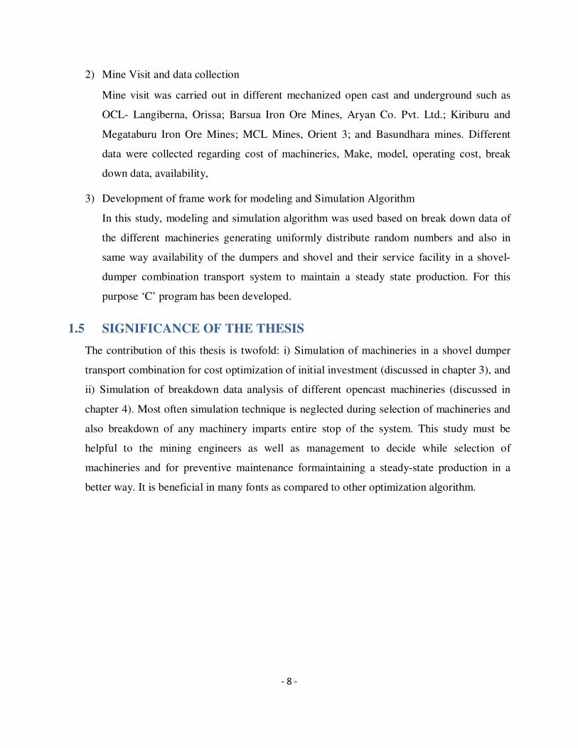
3) Development of frame work for modeling and Simulation Algorithm
In this study, modeling and simulation algorithm was used based on break down data of
the different machineries generating uniformly distribute random numbers and also in
same way availability of the dumpers and shovel and their service facility in a shovel-
dumper combination transport system to maintain a steady state production. For this
purpose ‘C’ program has been developed.
1.5 SIGNIFICANCE OF THE THESIS
The contribution of this thesis is twofold: i) Simulation of machineries in a shovel dumper
transport combination for cost optimization of initial investment (discussed in chapter 3), and
ii) Simulation of breakdown data analysis of different opencast machineries (discussed in
chapter 4). Most often simulation technique is neglected during selection of machineries and
also breakdown of any machinery imparts entire stop of the system. This study must be
helpful to the mining engineers as well as management to decide while selection of
machineries and for preventive maintenance formaintaining a steady-state production in a
better way. It is beneficial in many fonts as compared to other optimization algorithm.

- 9 -
Chapter 2
LITERATURE REVIEW
2.1 INTRODUCTION
An extensive literature survey was done in order to approaches adapted by the researches in
the past. The literatures reviewed in the present research may be categorized according to their
approaches to solve mine production scheduling problem using mathematical models as
deterministic models, which always yields the same output for fixed input values, but in this
research it is shown either in case of breakdown of machineries which is uncertain in nature, so
uniformly random numbers are created as input and the result or outputs are categorized in
such a manner that in future it can be sort out from their particular category before further
sudden breakdown. Thus it is minimized to maintain a steady state production. Also in case of
service facility of a shovel and arrival of a dumper is uncertain in nature, so uniformly
distributed random numbers are generated as input to the models. Thus output is minimization of
waiting time of both shovel and dumper to reduce the cost of investment of the machineries. It
optimizes the net present value of the profits over the life of the mine.
2.2 DETERMINISTIC MODELS OF MINE PRODUCTION SCHEDULING:
Using of different mathematical models for mine production scheduling is extensively
surveyed. The introduction of the concept of linear programming for optimization of mine
production scheduling was made by Johnson (1969). He used linear programming to determine a
feasible extraction sequence which ultimately maximized the total profits over the planning
horizon. A dynamic cut-off grade strategy was applied to determinate between ore and waste in a
mineral deposit and this cut-off change with time. The scheduling problem was formulated as a
large scale linear programming problem considering governing constraints of the system and
further by applying decomposition principle, the problem was decomposed into simple linear
programming problem, called the master problem and set of sub-problem was relatively simple.

- 10 -
Gershon (1982) also applied the linear programming approach to schedule mining operation in a
optical manner. He presented cases in which linear programming was applied in three different
mines which include a copper, a coal and a limestone mine. He developed and presented a mine
scheduling optimization (MSO) approach. This system, which optimizes the net present value of
the profit over the life of mine, considers multiple pits, poly-metallic ores ore handling and
processing facilities, environmental limitation and product sales[1,3]. MSO represents advances
in the state-of-the-art of linear programming applications to mine scheduling in five areas such as
scope and generality of the problem addressed, model formulation, computational requirements
and the long-term and short term interfaces. Generalized in its organization, this approach was
applicable to a wide variety of mining operations. Wilke et al. (1984) employed a simulation
algorithm in conjunction with linear programming to determine the long-term and medium-term
production schedules. They used simulation for handling geometric and equipment restrictions,
and linear programming for determining optimum ore and waste handling over time horizon
[5,11].
K. C. Brahma, B. K. Pal & C. Das (2008) attempt to throw some light on mine automation using
the concept of Petri Nets. The drilling operation in an opencast mine with double rod drilling
provision has been considered for analysis and has been simulated [23,27]. They shows Petri Net
based modeling of drilling operation is a simple and effective method that can provide an insight
to the academicians and mine managers to further develop a more refined and realistic time and
cost estimates for complex opencast mine projects. The Petri Nets can be applied for automation
in mining technology in an environment friendly and safe manner so that zero accident potential
(ZAP) can be achieved. Temporary machine failures can be averted with better simulation which
can be updated time and again reducing the break down hours to minimum [12,35].
T. Cichon (1998) developed computer techniques and resultant increased speed and accuracy of
calculation carried out, easy graphic representation of design and its duplication, quick creation
and processing of databases and also, their searching, further treatment of graphic files,
possibility to create spatial model of design facility, its visualization, archive of data, brought
about an interest in aiding of mine planning by specialized computer programs. Computer
software is used as micro station, Intergraph, I/Mine modeler, Intrasoft MX Foundation (MOSS),
Data mine Studio, Auto CAD or commonly used MS Office package [24,25].
- 11 -
U. A. Dzharlkaganov, D. G. Bukeikhanov & M. Zh. Zhanasov (2004) presented of automated
forming of perspective and current plans of mining operations development when open mining
of complex structural multi-components iron-ore and poly-metallic deposits. It includes two
programming functional complexes (modules): optimizing and interactive [13, 22].
It shows joint using of two modules with different ideology and principles of operation in
one system of computer aided design and planning of mining operations at opencasts allows
substantially increasing quality and decreasing duration of decision making [19, 20].
Also by using the first module of optimization calculations and construction of contours of
mining operations in package regime we receive the most priority directions of moving of
mining operations by working levels. It allows substantially decreasing time of a search of
optimal contours of mining operations up to the end of planned period [14, 28].
The second module is used for taking final decision in interactive regime and allows more
adequate taking into account possible complex situations. It may be used in addition to
operations of the first module or as independent apparatus for current and timely planning of
mining operations [15, 26].
For taking correct decision it is important to ensure a forenamed subsystems with reliable
information about interaction of parameters and indexes of operation of opencast in different
mining-technical and technological conditions with the help of spatial recognizing algorithm and
formulae [18, 29].
Using of different mathematical models for mine production scheduling is extensively
surveyed. The introduction of the concept of linear programming for optimization of mine
production scheduling was made and elaborated [9, 10]. They used linear programming to
determine a feasible extraction sequence which ultimately maximized the total profits over the
planning horizon.
A dynamic cut-off grade strategy was applied to determinate between ore and waste in a
mineral deposit and this cut-off change with time. The scheduling problem was formulated as a
large scale linear programming problem considering governing constraints of the system and
further by applying decomposition principle, the problem was decomposed into simple linear
programming problem, called the master problem and set of sub-problem was relatively simple.

- 12 -
The drilling operation in an opencast mine with double rod drilling provision has been
considered for analysis and has been simulated [2, 37]. Computer techniques were applied for
design of dragline operation and its graphic representation for quick processing of databases was
developed [6, 16].
Also by using the first module of optimization calculations and construction of contours of
mining operations in package regime we receive the most priority directions of moving of
mining operations by working levels. It allows substantially decreasing time of a search of
optimal contours of mining operations up to the end of planned period [4, 36].
The second module is used for taking final decision in interactive regime and allows more
adequate taking into account possible complex situations. It may be used in addition to
operations of the first module or as independent apparatus for current and timely planning of
mining operations [8, 17].
For taking correct decision it is important to ensure a forenamed subsystems with reliable
information about interaction of parameters and indexes of operation of opencast in different
mining-technical and technological conditions with the help of spatial recognizing algorithm and
formulae [7, 21].

- 13 -
Chapter 3
METHODOLOGY
3.1 INTRODUCTION:
After mining company has got the lease of a mineral deposit, the problem is then how to
mine and process that deposit the best way. The principle problem facing managers or engineers
who must decide on mine plant site, equipment selection and long range scheduling is how one
can optimize a property not only in terms of efficiency but also as to project duration. For faster
rate of production mechanization at a high degree is obvious. With the advanced technology
different types of mechanization such as shovel, dumper, dozer, drill machine etc. Use of more
machineries leads to more complexity in operation and as result it is very difficult to make the
proper matching of those equipments. These Machineries are very costly. So unless they are
properly matched reduction in production cost is very difficult. Increase in idle times of
machineries leads to increase in production cost. In order reduce the idle time or waiting time.
The number of machineries may be increased. Due to higher cost of machineries more
investment is needed which ultimately contribute in higher production cost. So, unless you
getting a perfect matching with optimum number of equipments reduction in production cost is
impossible. So, it is needed to analyses the operations of equipments considering their break
down periods, repairing, maintenance of preventive maintenance, availability of spare-parts,
efficiencies of operators and management philosophy etc. This study is based on use Monte –
Carlo technique in operation of shovel- dumper combination.
The field of modeling and simulation is as diverse as the concern of the man. Every
discipline has developed, or is developing, its own models and its own approach and tools for
studying these models.
The necessary of simulation and modeling relies on the same reasoning that determined
that we should have acquired at least some grounding in mathematics. Nobody questions the role
of arithmetic in the sciences, engineering and management. Arithmetic is all pervasive, yet it is a

- 14 -
mathematical discipline having its own axioms and logical structure. Its content is not specific to
any other discipline but is directly applicable to them all.
The practice of modeling and simulation too is all pervasive. However, it has its own
concepts of modeling description, simplification, validation simulation and exploration, which
are not specific to any particular discipline. These statements are agreed to by all.
3.2 SYSTEM MODELING CONCEPT:
This is the key concept that underlies the framework and methodology for modeling and
simulation. The most basic concept is that of mathematical system theory. Which was first
developed in 1960s, this theory provides a fundamental, rigorous mathematical formalism for
representing dynamical system of mines loading system of shovel dumper combination and
various machineries breakdown statistics and their performances. There are two main,
orthogonal, aspects to the theory [30, 31].
1) Levels of system specification – These are the levels at which we can describe how
system behave and the mechanism that make the framework the way they do.
2) System specification formalism- These are the systems of modeling style, such
continuous or discrete, that modelers can use to build system models.
The theory is quite intuitive, it does present an abstract way of thinking about the world that we
will probably unfamiliar.
3.3 SYSTEM SPECIFICATION FORMALISM:
System theory distinguishes between systems structure which is the inner constitution of
a system and behavior which is its outer manifestation. Viewed as a black board system, the
external behavior of a system is the relationship it imposes between its input time histories and
output time histories. The system input /output behavior consist of the data of the pairs of the
data records which is input time segments paired with output time segments and gathered from a
real system or model . The internal structure of a system includes its state and state transition
mechanism (dictating how inputs transform current states into successor states) as well as the
state-to-output mapping. Knowing the system structure which allows us to deduce (analyze and
simulate) its behavior. Usually the other direction (interfering structure from behavior) is not

- 15 -
univalent- indeed, discovering a valid representation of an observed behavior is one of the key
concern of the modeling and simulation enterprise [32, 33].
SYSTEM
INPUT
OUTPUT
Figure 3.1: Basic system concepts
An important structure concept is that of decomposition , namely, how a system may be broken
down into component system, a second system is that of composition, i.e. how component
system may be coupled together to form a larger system. System theory is closed under
composition in that the structure and behavior of a composition of a system can be expressed in
the original system theory terms. The ability to continue to compose larger and larger
BLACKBOARD

- 16 -
Fig 3.2: Hierarchical system decomposition
- 17 -
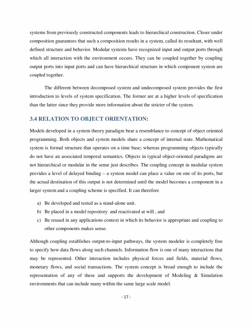
systems from previously constructed components leads to hierarchical construction. Closer under
composition guarantees that such a composition results in a system, called its resultant, with well
defined structure and behavior. Modular systems have recognized input and output ports through
which all interaction with the environment occurs. They can be coupled together by coupling
output ports into input ports and can have hierarchical structure in which component system are
coupled together.
The different between decomposed system and undecomposed system provides the first
introduction to levels of system specification. The former are at a higher levels of specification
than the latter since they provide more information about the stricter of the system.
3.4 RELATION TO OBJECT ORIENTATION:
Models developed in a system theory paradigm bear a resemblance to concept of object oriented
programming. Both objects and system models share a concept of internal state. Mathematical
system is formal structure that operates on a time base; whereas programming objects typically
do not have an associated temporal semantics. Objects in typical object-oriented paradigms are
not hierarchical or modular in the sense just describes. The coupling concept in modular system
provides a level of delayed binding – a system model can place a value on one of its ports, but
the actual destination of this output is not determined until the model becomes a component in a
larger system and a coupling scheme is specified. It can therefore
a) Be developed and tested as a stand-alone unit.
b) Be placed in a model repository and reactivated at will , and
c) Be reused in any applications context in which its behavior is appropriate and coupling to
other components makes sense.
Although coupling establishes output-to-input pathways, the system modeler is completely free
to specify how data flows along such channels. Information flow is one of many interactions that
may be represented. Other interaction includes physical forces and fields, material flows,
monetary flows, and social transactions. The system concept is broad enough to include the
representation of any of these and supports the development of Modeling & Simulation
environments that can include many within the same large scale model.

- 18 -
Although system models have formal temporal and coupling features not shared by coupling
features of conventional objects, object orientation does provide a supporting computational
mechanism for system modeling. Indeed there have been many object oriented implementations
of hierarchical modular modeling systems. These demonstrate that object-oriented paradigms,
particularly for distributed computing, can serve as a strong foundation to implement the
modular system paradigm [34].
3.5 SYSTEM FORMALISM EVALUATION:
As in many situations, portraying the evaluation of an idea may help understand the
complexities as they develop. The basic systems modeling formalism as they were presented in
the TMS76. This was first approaches to modeling as system specification formalism. This Is
shorthand means of delineating a particular system within a sub class of all systems. The
traditional differential equation systems, having continuous states and continuous time, were
formulated as the class of differential equation system specification (DESS). Also system that
operated on a discrete time base such as automata were formulated as the class of Discrete Time
System Specification (DTSS). In each of these cases, mathematical representation had proceeded
their computerized incarnations (Newton-Leibnitz).
However, the reverse was true for the third class, The Discrete Event System
Specification (DEVS). Discrete event models were largely prisoners of their simulation
language implementations or algorithmic code expressions. Indeed there was a prevalent belief
that discrete event “world views” constituted new mutant forms of simulation, unrelated to the
traditional mainstream paradigms. Fortunately, that situation has begun to change as the benefits
of abstractions in control and design became clear. Witness the variety of discrete event dynamic
system formalisms that have emerged.
While each one – examples are petri-nets, minimax algebra, and GSMP (Generalized
semi-Markov processes)- has its application area, none were developed deliberately as subclasses
of the system theory formalism. Thus to include such a formalism into an organized system-
theory-based frame-work requires “embedding” it into DEVS.
“Embedding”. It indicates subclass relationships; for example they suggest that DTSS is
subclass of DEVS. However, it is not literally true that any discrete time system is also discrete

- 19 -
event system (their time bases are distinct, for example). So, we need a concept of simulation
that allows us to say when one system can do the essential work of another. One formalism can
be embedded in another if any system in the first can be simulated by some system in the second.
Actually, more than one such relationship, or morphism may be useful, since, as already
mentioned, there are various levels of structure and behavior at which equivalence of the system
could be required.
System
dq/dt = a*q + bx
Simulator
Numerical Integer
DESS Model :
Fig3.3: System Specification Formalism

- 20 -
q (t + 1) = a * q (t) + b * x (t)
DTSS Model :
Simulator
Numerical Integer
Fig3.4: System Specification Formalism
System
Simulator Recursive

- 21 -
DESS Model :
Time to text event,
State at next event
Fig3.5: System Specification Formalism
As a case in point any DTSS could be simulated a DEVS by constraining in time advance
to be constant. However, this is not as useful as it could be until we can see how it applies to
decomposed systems. Until that is true, we either must reconstitute a decomposed discrete time
system to its resultant before representing it as a DEVS but we cannot network the DEVS
together to simulate the resultant.
3.6 COMBINATION OF CONTINUOUS AND DISCRETE FORMALISMS:
Skipping many years of accumulating developments, the next major advance in system
formalisms was the combination of discrete events and differential equation formalism into one,
the DEV&DESS. As shown in Fig: 4
SYSTEM
Simulator Numerical Integer

- 22 -
This formalism subsumes both the DESS and the DEVS (hence also the DTSS) and thus
supports the development of coupled system whose components are expressed in any of the basic
formalisms. Such multi-formalism modeling capability is important since the world does not
usually lend itself to using one form of abstraction at a time. For example, a chemical factory is
designed with discrete event formalisms. Also DEV & DESS were closed under coupling and in
order to do so, had to deal with the pairs of input-output interfaces between the different types of
systems. Closure under coupling also required that the DEV &DESS formalism provide a means
to specify components with intermingled discrete and continuous expressions. Finally, simulator
algorithms (so called abstract simulators) had to be provided to establish that the new formalism
could be implemented in computational form.
3.7 QUANTIZED SYSTEM:
Since parallel and distributed simulation is fast becoming the dominant form of model
execution, and discrete event concepts best fit with this technology, our focus is on a concept
called the DEV bus. This concept, introduced in 1996 concerns the use of DEVS models as
“wrappers” to enable a variety of models to interoperate into a networked simulation. It is
particularly germane to the high level architecture defined by United States Department of
Defense. One way of looking at this idea is that we want to embed any formalism, including, for
example, the DEV & DESS, into DEVS. Another way is to introduce a new class of systems,
called quantized system, as illustrated in Fig: 6. In such systems, both the input and output are
quantized. As an example, an analog-to-digital converter does such quantization by mapping a

- 23 -
SYSTEM
DESS DEVS
Differential Equation Discrete Event
System Specification System
Specification
DTSS
Discrete Time System Specification
Fig: 3.6 The Dynamics of Basic System Classes
real number into a finite stringed of digits. In general, quantization forms equivalence classes of
outputs that then become indistinguishable for downstream input receivers, requiring less data
network bandwidth, but also possibly incurring error.

- 24 -
SYSTEM
DEVS & DESS
Discrete Event & Differential Equation
System Specification
DESS DEVS
Differential Equation Discrete Event
System Specification System Specific
DTSS
Discrete Time System Specification
Fig: 3.7 Introducing the DEV & DESS Formalism
3.8 EXTENSION OF DEVS:
Various
extensions of DEVS have been developed as illustrated in Fig: 7. These developments expand
the classes of system models that can be represented in DEVS, and hence, integrated within both
the DEVS bus and the parent systems theory formalism.

- 25 -
SYSTEM
DEVS & DESS DEVS
QUANTIZED
SYSTEM
DISCRETIZED
SYSTEM
QUANTIZED DESS
DESS DISCRETIZED DESS
DESS
LEGEND
subclass
exact
as close as desired
Fig 3.8: Introducing quantized system
- 26 -
PARALLEL/CONFLUENT
DEVS
SYMBOLIC DYNAMIC
DEVS STRUCTURE
DEVS
DEVS
FUZZY REAL TIME
DEVS DEVS
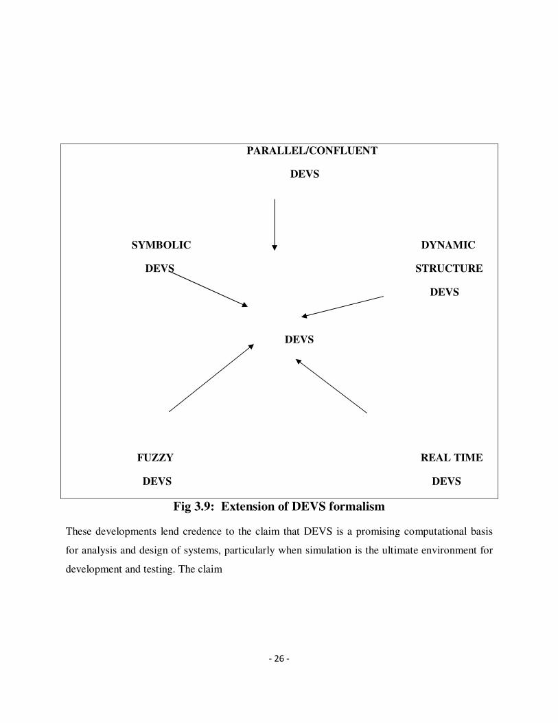
Fig 3.9: Extension of DEVS formalism
These developments lend credence to the claim that DEVS is a promising computational basis
for analysis and design of systems, particularly when simulation is the ultimate environment for
development and testing. The claim

- 27 -
DEVS REPRESENRED
SYSTEM
UNIVERSALITY OF
DEVS
REPRESENTATION
QUANTIZED
SYSTEM
UNIQUENESS OF
COMPUTATIONAL
DEVS AS DEDS BASIS FOR
SIMULATION,
REPRESENTATION DESIGN,
CONTROL
DEVS
Fig 3.10: DEVS as a Computational basis for Simulation, Design and Control.
rests on the universality of the DEVS representation, namely the ability of DEVS bus to support
the basic system formalism. DEVS is the unique form of representation that underlies any system
with discrete event behavior. This uniqueness claim of DEVS, offers the promise that the
profusion of discrete event formalisms under development for control and management of

- 28 -
systems can be embedded as sub formalisms of DEVS in the DEVS bus and thus made
accessible in an integrated distributed simulation environment.
3.9 LEVELS OF SYSTEM KNOWLEDGE:
The system specification hierarchy is the basis for a frame work for M & S which sets forth
the fundamental entities and relationships in the M & S enterprise. The hierarchy is first
presented in an informal manner and later, in its full mathematical rigor. This presentation is a
review of George Klir’s system framework.
Table 1 identifies four basic levels of knowledge about a system recognized by Klir. At each
level we know some important things about a system that we did not know at lower levels. At the
lowest level, the source level identifies a portion of the real world that we wish to model and the
means by which we are going to observe it. As the next level, the data level is a data base of
measurements and observations made for the source system. When we get to level 2, we have
ability to recreate this data using a more compact representation, such as a formula. Since,
typically, there are many formulae or other means to generate the same data, the generative level,
or particular means or formula we have settled on, constitutes knowledge we did not have at the
data system level. About the models in the context of simulation studies they are usually
referring to the concepts identified at this level. That is, to them a model means a program to
generate data. At the last level, the structural level, we have a specific kind of generative system.
In other words, we know how to generate the data observed at the level 1 in a more specific
manner-in terms component system that are interconnected together and whose interaction
accounts for the observation made. Systems are often referring to this level of knowledge. The
whole is the sum (or as some times claimed, more or less than the sum) of its part. The term
“subsystem” is also use for these parts, and then they call component systems (and reserve the
subsystem for another meaning).
Klir’s terms are by no means universally known, understood, or accepted in the M & S
community. However, his frame work is a useful starting point since it provides a unified
perspective on what are usually considered to be distinct concepts. From this perspective, there
are only three basic kinds of problems dealing with systems and they involve moving between
the levels of system knowledge (table-2). In systems analysis, we are trying to understand the
behavior of an existing or hypothetical system based on its known structure. System inference is

- 29 -
done when do not know what this structure is-so we try to guess this structure from observation
that we can make. Finally, in system design, we are investigating the alternative structures for a
completely new system or the design of an existing one.
The central idea is that when we move to a lower level, we do not generate any really new
knowledge-we are only making explicit what is implicit in the description we already have.
Making something explicit can lead to insight, but it is a form of new knowledge, but Klir is
considering this kind of subjective (or modeler-dependent) knowledge. In this M & S context,
one major form of systems analysis is computer simulations which generate data under the
instructions provided by a model. Although no new knowledge is generated, interesting
properties may come to light of which we were not aware before the analysis. On the other hand,
system inference, and system design are problems that involve climbing up the levels. In both
cases, we have a low level system description and wish to come up with an equivalent higher
level one. For system interference, the lower level system is typically at the data system level,
being data that we have observed from some existing source system. We are trying to find a
generative system, or even a structure system, that can recreate the observed data. In the M & S
context, this is usually called model construction. In the case of system design, the source system
typically does not yet exist and our objective is to build one that has a desired functionality. By
functionality we mean that we want the system to do; typically, we want to come up with a
structure system, whose components are technological, i.e., can be obtained off-the-shelf, or built
from scratch from existing technologies. When these components are interconnected, as
specified by a structure system coupling relation, the result should be a real system that behaves
as desired.
It is very interesting that the process called reverse engineering has elements of both
interface and design. To reverse engineering an existing system, such as was done in the case of
the cloning of IBM compatible PCs, an extensive set of observations is first made. From these
observations, the behavior of the system is inferred and an alternative structure to realize this
behavior is designed-thus bypassing patent rights to the original system design.

- 30 -
Table3.1: Levels of System Knowledge
Level Name What we know at this Level
0 Source What variable to measure and how to observe them
1 Data Data collected from a source system
2 Generative Means to generate data in a data system
3 Structure Components (at lower levels) coupled together to form a
generative system
3.10 INTRODUCTION TO THE HIERARCHI OF SYSTEM SPECIFICATION:
At about the same time ( Klir 1970 ) he introduced epistemological (knowledge) levels, TMS76
formulated a similar hierarchy that is more oriented toward the M & S context. This framework
employs a general concept of dynamical system and identifies useful ways in which such a
system can be specified. These ways of describing a system can be ordered in levels as in table 3.

- 31 -
Table 3.2: Fundamental Systems Problems
System
Problems
Does source of the data exist? We are
trying to learn about it.
Which levels transition is involved
System
analysis
The system being analyzed may exist or may
be planned. In either case we are trying to
understand its behavioral characteristics.
Moving from higher to lower levels,
e.g. using generative information to
generate the data in a data system.
System
inference
The system exists. We are trying to infer
how it works from observations of its
behavior.
Moving from lower to higher levels,
e.g., having data, finding a means to
generate.
System
design
The system being designed does not yet exist
in the form that is being completed. We are
trying to come up with a good design for it.
Moving from to lower levels, e.g.,
having a means to generate observed
data, synthesizing it with compo-
nent taken off the shelf.
3.11 SIMULATION
Simulation is a numerical technique for conducting experiments that involves certain types of
mathematical and logical relationship necessary to describe the behavior and structure of a
complex real world system over extended period time.
According to Shannon “Simulation is the process of designing a model of a real system and
conducting experiments with this model for the purpose of understanding the behavior (within
the limits imposed by a criterion or a set of criteria) for the operation of the system”.
Using Simulation, an analyst can introduce the constants and variables related to the problem, set
up the possible courses of action and establish criteria which act as measures of effectiveness.

- 32 -
Table 3.3: System Specification Hierarchy
Levels Specification
Name
Correspondence to
Klir’s
What we know at this level
0
Observation
Frame
Source System
How to stimulate the system with inputs;
What variables to measure and how to
observe them over a time base;
1
I/O behavior
Data System
Time index data collected from a source
system; consist of input/output pairs.
2
I/O function
--
Knowledge of initial state; given an initial
state, every input stimulus produces a unique
output.
3
State
Transition
Generative System
How states are affected by inputs; given a
state and what is the state after the input
stimulus is over; what output vent is
generated by a state.
4
Coupled
Component
Structure System
Components and how they are coupled
together. The components can be specified at
lower levels or can even be structure systems
themselves-leading to hierarchical structure.
3.12 REASONS FOR ADOPTING SIMULATION:
a) It is an appropriate tool for solving a business problem when experimenting on the real
system would be too expensive.
b) It is a desirable tool when a mathematical model is too complex to solve and is beyond
the capacity of available personnel. And is not detailed enough to provide information on
all important decision variables.
c) It may be the only method available, because it is difficult to observe the actual reality.

- 33 -
d) Without appropriate assumption, it is impossible to develop a mathematical solution.
e) It may be too expensive to actually observe system.
f) There may not be sufficient time to allow the system to operate for a very long time.
g) It provides trial and error movements towards the optical solution. The decision maker
selects an alternative, experience the effect of the selection, and then improves the
selection.
3.13 TRANSPORT SYSTEM:
Mine transport may be of truck, railway, and conveyor belt and skip transport. In truck
transport, the output from a truck in an hour
q = 60 c.f/T and T = t1 + tf + tb + td + ts
where t1 = c/α. Vsh. Fsh. * tsh Tf = df/Vf ; tb = db/Vb
The face output per hour (Q) = K.q.n = K.60.c.f.n/T
Output from the mine per day = m.K.60.c.f.n/T *2*6
Considering 2 shifts production and 6 hours effective working in a shift
Generally for the face output average utilization and net utilization are considered.
Average utilization = Availability/Schedule hour
= (Schedule hour – Breakdown period)/Schedule hour
= 1 – (Breakdown/Schedule hour)
Net utilization = Utilization hour/Schedule hour = (Availability – Idle Time)/Schedule hour
= 1 – (Breakdown period/Schedule hour) – (Idle Time/Schedule hour)
As the average and net utilization are much lesser than 100% so the production was
hampered. Idle time is minimized by preparing Queuing models by considering haul distance,
loading capacity of the dumper, capacity of the crusher, upward and downward slope
minimization, etc.

- 34 -
3.14 FACE OUTPUT AND PRODUCTION COST RELATIONSHIP
Production cost per ton of mineral consist of two main groups of expenditure
i) Relative capital expenditure, CE = Ic/Qc, higher is the capacity of the mine, higher is
the capital investment for construction.
ii) Relative revenue expenditure, RE = TRE/Qc, higher is the capacity is the mines lower
is the revenue expenditure for per ton of mineral production.
A simulation model was viewed as a set of components that interact. These interactions of
the components were most generally parallel in nature as opposite to a sequential one. In
parallel interaction, may action were occurred simultaneously. Thus one of the essential tusks
of current simulation languages was to enable the computer, which acted sequentially one
step at a time.
3.15 SIMULATION MODELS
To minimize breakdown period it was badly needed to analyze them statistically by the
simulation model, viz.
(i) Generation of uniformly distributed random numbers,
(ii) Generation of normally distributed random numbers
(iii) System simulation to event types analysis,
(iv) Identification of event by statistically distribution
3.16 UNIFORMLY DISTRIBUTED RANDOM NUMBERS
It was generated by multiplicative congruential generator or power residue generator
(Fig……….) which consisted of
XI+1 = X1 * a (modulus M)
In the present work was done by
XI+1 = 24298 Xi + 9991 mod 199017
Ri+1 = Xi+1/m = Xi+1 / 199017
Xo = 199017 * Ro
- 35 -
3.17 NORMALLY DISTRIBUTED RANDOM NUMBER
These are the numbers where the probability of all the number not same. As such there was
no specific table to those numbers and were generally made by converting the uniformly
distributed random numbers with the help of a computer. There is lot of procedure for this
conversation. Mostly computation was done like this:
Let, the independently and identically distributed random variables are X1, X2, X3……. Xd
for
U (0, 1) and mean of those numbers is X.
So for U (0, 1), Expectation (E) = ½ and
Variance (V) = 1/12d and by Central Limit Theorem
X = N (E(x), v(x)) = N (1/2, 1/√12d)
Or (x-1/2) √ 12d = N (0,1)
Thus n observed from uniform gives 1, obs. From normal. The conversion procedure which
was used for solving these work are :
If R4 was a normally distributed random number (RN) with mean (µ) = 0 and standard
deviation (σ) = 1 then conversation was done [Fig………] by
RN = R4.σ + µ
where R4 = √ [-2.In.R2] * cos [2π R3]
3.18 SYSTEM SIMULATION ON EVENT TO EVENT ANALYSIS
Different sub-routine for different were prepared in this simulation model and the sub-
routines were design based on the frequency distribution of different breakdown which
occurred in the mine. The duration of each breakdown was analyzed and from the cumulative
frequency distribution the randomizing cases were drawn because breakdown of different
equipments could not follow a particular rule. So, by generating the uniform ally distributed
random numbers and then converting them to a normally distributed one, it aws possibly to

- 36 -
tell which event could come first and so on. Though case arose also a particular event
occurred twice at a time. As a result, event analyses were needed for this present simulation.
3.20 EVENT IDENTIFICATION
This means to determine event which would come first, second and so on. In the present
work 8 events were considered demarcating by 1, 2, 3…. 8 when breakdown of any
equipment took place in the mine, and rectifying this breakdown another one went out-of-
order. By statistical distribution, it was identified that which event might be from the rest
event. A clock schedule of the activity was maintained and a stimulatory list was prepared
from the distribution function. If more than one event was scheduled to be executed, the tie
breaking rules specified by the SELECT function was determined to identify the event
actually executed. For the identification of this events, a special; event sub-routines was
prepared which followed the different event sub-routine and the frequency distribution help
to prepare this identification.
3.21 SUB ROUTINE SKEWING OF UNIFORMALLY DISTRIBUTED
RANDOM NUMBER
Mine data were analyzed and from the data histogram were prepared [Table i-iv]. It was seen
that for 8 different events breakdown in the plant production was hampered. This breakdown
events were not uniform ally distributed, there frequency distribution were also different.
Once first event was broken down, did not mean that in the ninth term it could be broken
down. This irregularities were following the normally distribution curves and there histogram
were not showing smooth curves. The mean of the frequency curve was right to the mode
and just reverse was also not impossible. These 8 events subroutine skewing of, was replaced
to the uniform ally distributed random numbers to the histogram, the solution of the problem
of much easier than the problem which were dealt in this paper.
3.22 SIMULATION OF CONTINUOUS SYSTEMS:
From the viewpoint of simulation there are two fundamentally different types of systems:
1) Systems in which the state changes smoothly or continuously with time (continuous systems).
2) Systems in which the state changes abruptly at discrete points in time (discrete systems).

- 37 -
Usually, the simulation of most systems in engineering and physical sciences turns out to be
continuous, whereas most systems encountered in operations research and management sciences
are discrete. The methodologies of discrete and continuous simulations are inherently different.
Continuous dynamic systems, those systems in which the state or the variables vary continuously
with time, can generally be described by means of differential equations. If the set of
(simultaneous) differential equations describing a system are ordinary, linear, and time –
invariant (i.e. have constant coefficients), an analytic solution is usually easy to obtain. In
general differential equations of a more difficult nature can only be solved numerically.
Simulating the system often gives added insight into the problem besides giving the required
numerical solution.
3.23 SELECTING SIMULATION SOFTWARE
Overview of the Steps Involved in Selecting Simulation Software
The steps for selecting simulation software are outlined below (and detailed in subsequent
sections):
1. Establish the commitment to invest in simulation software to solve your problem.
2. Clearly state the problem (or class of problems) that you would like to solve.
3. Determine the general type of simulation tool required to solve the problem.
4. Carry out an initial survey of potential solutions.
5. Develop a list of functional requirements.
6. Select the subset of tools that appear to best meet the functional requirements.
7. Carry out a detailed evaluation of the screened tools and select a solution.
Step 1: Establish the Commitment to Invest in Simulation Software
Before spending any effort to research simulation tools, the organization should establish the
commitment to invest both the necessary money and staff time into purchasing and learning how
to use a simulation software program. Depending on the type of simulation tool selected, the 15

- 38 -
price for a single license is likely to be no less than Usually, the simulation of most systems in
engineering and physical sciences turns out to be continuous, whereas most systems encountered
in operations research and management sciences are discrete. The methodologies of discrete and
continuous simulations are inherently different. Continuous dynamic systems, those systems in
which the state or the variables vary continuously with time, can generally be described by
means of differential equations. If the set of (simultaneous) differential equations describing a
system are ordinary, linear, and time –invariant (i.e. have constant coefficients), an analytic
solution is usually easy to obtain. In general differential equations of a more difficult nature can
only be solved numerically. Simulating the system often gives added insight into the problem
besides giving the required numerical solution.
Step 2: Clearly State the Problem You Wish to Address
Perhaps the most important step in selecting simulation software is to clearly state the problem
(or class of problems) that you would like to address. This must include a general statement of
what you would like the simulation tool to do. Without doing so, it will be impossible to
determine, first, the type of simulation tool you should look for, and subsequently, to list the
functional requirements and desired attributes of the tool. To illustrate what is required, several
examples of simulation problem statements are listed below:
Managing the water supply for a city:
Managing a water supply is difficult due to the dynamic (and naturally unpredictable) nature of
the problem (resulting from uncertainties in both weather and demand). The simulation tool must
be able to predict the movement of water through a system (e.g., reservoirs, distribution systems)
tracking the quantities and flow rates at various locations. It must be able to quantitatively
represent the inherent uncertainty in the system (due to the uncertainty in the weather and
demand), and represent various management options (e.g., rules for allocating flows under
specified 16 conditions).
The output of the simulation will consist of probabilistic predictions of daily water levels and
flow rates over time given a specified management alternative. Carrying out a risk analysis for a
complex mission (i.e., a machine and/or persons performing a specified task or set or tasks):

- 39 -
Carrying out a risk analysis for a complex mission is difficult due to the complex interactions
and dependencies of the various components, and the fact that the environment may evolve
dynamically during the mission. The simulation tool must be able to simulate the operation of the
machine throughout the mission, explicitly modeling component interactions, dependencies and
failures. It must also be able to represent the impact of a changing environment on the
components. The output of the simulation will consist of probabilities of failure (and success) for
a mission of specified length, and identification of key failure mechanisms.
Modelling the financial outcome of several alternative projects:
When selecting or ranking various alternative projects or undertakings, it is necessary to
quantitatively evaluate both the costs and revenues associated with each project. The simulation
tool must be able to simulate the future costs and revenues associated with alternative projects,
explicitly accounting for the uncertainty in costs, durations and revenues. The simulation must be
able to represent disruptive events (e.g. strikes, price changes) and resulting contingency plans
that allow a simulated project to respond to new developments in a realistic way. The output of
the simulation will consist of probabilistic predictions of the NPV and IRR for each alternative.
Note that these statements are not extremely detailed, but provide a clear statement of the
problem, a general statement of what processes and features must be included, and what the
output of the simulation will be. This provides enough information to direct a survey of potential
solutions and carry out an initial screening. In a later step in the process, more detailed
requirements will need to be defined in order to differentiate between the available options.
Step 3: Determine the General Type of Simulation Tool Required
Because simulation is such a powerful tool to assist in understanding complex systems and to
support decision-making, a wide variety of approaches and tools exist. Before trying to survey all
available tools, you must first decide upon the general type of tool that you require. 17 There are
a variety of simulation frameworks, each tailored for a specific type of problem. What they all
have in common, however, is that they allow the user to model how a system might evolve or
change over time. Such frameworks can be thought of as high-level programming languages that
allow the user to simulate many different kinds of systems in a flexible way. Perhaps the
simplest and most broadly used general purpose simulator is the spreadsheet. Although
- 40 -
spreadsheets are inherently limited in many ways by their structure (e.g., representing complex
dynamic processes is difficult, they cannot display the model structure graphically, and they
require special add-ins to represent uncertainty), because of the ubiquity of spreadsheets, they are
very widely used for simple simulation projects (particularly in the business world). Other
general purpose tools exist that are better able to represent complex dynamics, as well as provide
a graphical mechanism for viewing the model structure (e.g., an influence diagram or flow chart
of some type). Although these tools are generally harder to learn to use than spreadsheets (and
are typically more expensive), these advantages allow them to realistically simulate larger and
more complex systems. The general purpose tools can be broadly categorized as follows:
Discrete Event Simulators: These tools rely on a transaction-flow approach to modeling
systems. Models consist of entities (units of traffic), resources (elements that service entities),
and control elements (elements that determine the states of the entities and resources). Discrete
event simulators are generally designed for simulating processes such as call centers, factory
operations, and shipping facilities in which the material or information that is being simulated
can be described as moving in discrete steps or packets. They are not meant to model the
movement of continuous material (e.g., water) or represent continuous systems that are
represented by differential equations.
Agent-Based Simulators: This is a special class of discrete event simulator in which the mobile
entities are known as agents. Whereas in a traditional discrete event model the entities only have
attributes (properties that may control how they interact with various resources or control
elements), agents have both attributes and methods (e.g., rules for interacting with other agents).
An agent-based model could, for example, simulate the behavior of a population of animals that
are moving around and interacting with each 18 character.
Continuous Simulators: This class of tools solves differential equations that describe the
evolution of a system using continuous equations. Although these tools usually have some
mechanism to represent discrete events, they are most appropriate if the material or information
that is being simulated can be described as evolving or moving smoothly and continuously,
rather than in infrequent discrete steps or packets. For example, simulation of the movement of
water through a series of reservoirs and pipes can most appropriately be represented using a

- 41 -
continuous simulator. Continuous simulators can also be used to simulate systems consisting of
discrete entities if the number of entities is so large that the movement can be treated as a flow.
Hybrid Simulators: These tools combine the features of continuous simulators and discrete
simulators. That is, they solve differential equations, but can superimpose discrete events on the
continuously varying system. This can be useful, for example, in business simulations, in which
information and material can be modeled as moving continuously, but discrete financial
transactions also need to be represented Before starting your search for a simulation tool, you
should first determine which of these types of tools is required to solve your problem. In most
cases, this can be determined from the problem statement. If you are unsure, you should seek
input from someone who is familiar with simulation modeling (e.g., a consultant). One of the
worst mistakes you can make is to select the wrong type of tool (e.g., to select a continuous
simulator, when what you really need is a discrete event simulator).
Step 4: Carry Out an Initial Survey of Potential Solutions
Once you have selected the general type of tool you will need, you can then carry out an initial
survey to try to identify the possible options. Note that this process does not involve actively
evaluating any software tools. It is simply a survey to see what options are available. The only
screening that should be carried out should be based on general type. For example, if you have
determined that a continuous simulation tool is required, you should screen out pure discrete
event simulators. 19
This initial list of candidate tools can be generated from a variety of sources, including web
searches, peer recommendations, advertisements in trade magazines, and vendor lists from trade-
shows.
Step 5: Develop a List of Functional Requirements
Step 5 involves developing a set of functional requirements that you would like the software tool
to have. This list will then be used in a subsequent step to compare and contrast the candidate
solutions and filter out all but the most promising candidates. A functional requirement is a
necessary feature or attribute of the simulation software solution. Note that requirements specify
what the simulation software will do, not how. They should be as concise as possible. You
should also note whether a requirement is mandatory or simply desired (e.g., "must have" in a
- 42 -
requirement could indicate mandatory; "should have" could indicate desired, but not mandatory).
In order to develop a list of requirements, you generally start with your problem statement, and
describe the minimum set of functionality that will be necessary in order for the software to solve
your problem. The actual users of the software will be the primary developers of the
requirements list, but other stakeholders should also be involved, such as the ultimate client for
the model (e.g., a manager) and IT personnel, as they may have their own requirements. To
illustrate what is meant by a functional requirement, let's consider the first example problem
statement listed in the description of Step 2 above: Managing the water supply for a city:
Managing a water supply is difficult due to the dynamic (and naturally unpredictable) nature of
the problem (resulting from uncertainties in both weather and demand). The simulation tool must
be able to predict the movement of water through a system (e.g., reservoirs, distribution systems)
tracking the quantities and flow rates at various locations. It must be able to quantitatively
represent the inherent uncertainty in the system (due to the uncertainty in the weather and
demand), and represent various management options (e.g., rules for allocating flows under
specified conditions). The output of the simulation will consist of probabilistic predictions of
daily water levels and flow rates over time given a specified management alternative. …..20
The list of functional requirements for this problem statement would likely include the following
mandatory requirements:
• Must be able to track and conserve the continuous movement of material through a system
(in this case water).
• Must be able to represent random discrete changes to the system (e.g., pump failures)
• Must be able to represent stochastic processes (e.g., rainfall).
• Must be able to represent rules for allocating and splitting flows.
• Must be able to enter time series inputs.
• Must be able to import time series inputs and other data from spreadsheets.
• Must support Monte Carlo simulation.
• Must have a user interface that supports creation of transparent, well-documented models.
Desired (but perhaps not mandatory) requirements might include:
• Should be able to easily handle unit conversions
• Should be able to support distributed processing (for Monte Carlo simulation).

- 43 -
• Should support optimization.
• Should provide tools for sensitivity analysis.
Step 6: Select the Subset of Tools that Appear to Best Meet the Functional Requirements
Once you have defined your functional requirements, the next step is to apply the requirements,
to the candidate solutions, identifying and eliminating candidates that do not meet the mandatory
requirements.
Note that this step should not require downloading and running the candidate software. Instead,
the reviewer should be able to gather sufficient information to develop informed yes/no answers
to the requirements based on the vendors web pages, quick tours, animated demos, white papers,
case studies, recorded webinars, and in some cases, phone calls with technical sales
representatives. If you cannot easily gather information about a software product, it is
recommended that you eliminate that product from consideration (as this is generally an
indication that the quality of the product and/or the level of support is likely to be poor).
The output of this step is a list of viable solutions, each one of which will then be evaluated in
greater detail in the next step.
Step 7: Carry out a Detailed Evaluation of the Screened Tools
The final step in the process involves carrying out a detailed evaluation of the tools screened in
Step 6 and selecting the most appropriate tool. To do so, you should obtain an evaluation version
of each product and experiment with the software yourself. Although this is necessary, it can be
time-consuming, since each product will have a learning curve.
3.24 DISCRETE SYSTEM SIMULATIONS: In this type of system the changes are
discontinuous. Each change in the state of system is called an event. For example, arrival or
departure of a customer in a queue is an event. Likewise, sale of an item from the stock or arrival
of an order to replenish the stock is an inventory system. Arrival of a car at an intersection is an
event if we are simulating street traffic. Therefore, the simulation of a discrete system is often
referred to as discrete event simulation. It is commonly used by operations research workers to
study large, complex systems which do not lend themselves to a conventional analytic approach.
Some other examples are the study of sea and air ports, steel melting shops, telephone
exchanges, production line, stock of goods scheduling of projects, to name a few. Discrete

- 44 -
system simulation is more diverse and has less of a theory than continuous system simulation.
There are no overall sets of equation to be solved in discrete – event simulation.
FIXED TIME STEP VS EVENT-TO-EVENT MODEL:
In simulating any dynamic system – continuous or discrete – there must be a mechanism for the
flow of time. For we must advance time, keep track of the total elapsed time, determine the state
of the system at the new point in time, and terminate the simulation when the total elapsed time
equals or exceeds the simulation period. In simulation of discrete systems, there are two 22
fundamentally different models for moving a system through time: the fixed time step model and
the event-to-event (or next event) model. In a fixed time-step model a “timer” or “clock” is
simulated by the computer. This clock is up-dated by a fixed time interval, and the system is
examined to see if any event has taken place during this time interval (minutes, hours, and days,
whatever.). All events that take place during this period are treated as if they occurred
simultaneously al the tail end of this interval. In a next event simulation model the computer
advances time to the occurrence of the next event. It shifts from event to event. The system state
does not change in between. Only those points in time are kept track of when something of
interest happens to the system.
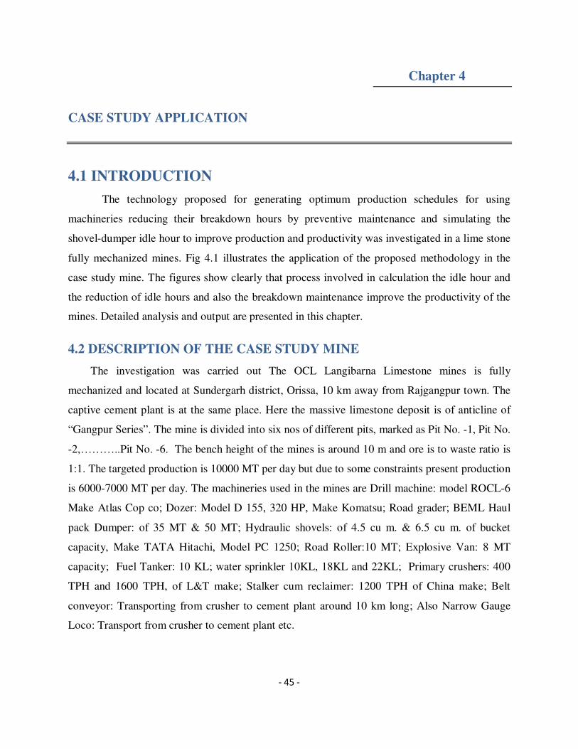
- 45 -
Chapter 4
CASE STUDY APPLICATION
4.1 INTRODUCTION
The technology proposed for generating optimum production schedules for using
machineries reducing their breakdown hours by preventive maintenance and simulating the
shovel-dumper idle hour to improve production and productivity was investigated in a lime stone
fully mechanized mines. Fig 4.1 illustrates the application of the proposed methodology in the
case study mine. The figures show clearly that process involved in calculation the idle hour and
the reduction of idle hours and also the breakdown maintenance improve the productivity of the
mines. Detailed analysis and output are presented in this chapter.
4.2 DESCRIPTION OF THE CASE STUDY MINE
The investigation was carried out The OCL Langibarna Limestone mines is fully
mechanized and located at Sundergarh district, Orissa, 10 km away from Rajgangpur town. The
captive cement plant is at the same place. Here the massive limestone deposit is of anticline of
“Gangpur Series”. The mine is divided into six nos of different pits, marked as Pit No. -1, Pit No.
-2,………..Pit No. -6. The bench height of the mines is around 10 m and ore is to waste ratio is
1:1. The targeted production is 10000 MT per day but due to some constraints present production
is 6000-7000 MT per day. The machineries used in the mines are Drill machine: model ROCL-6
Make Atlas Cop co; Dozer: Model D 155, 320 HP, Make Komatsu; Road grader; BEML Haul
pack Dumper: of 35 MT & 50 MT; Hydraulic shovels: of 4.5 cu m. & 6.5 cu m. of bucket
capacity, Make TATA Hitachi, Model PC 1250; Road Roller:10 MT; Explosive Van: 8 MT
capacity; Fuel Tanker: 10 KL; water sprinkler 10KL, 18KL and 22KL; Primary crushers: 400
TPH and 1600 TPH, of L&T make; Stalker cum reclaimer: 1200 TPH of China make; Belt
conveyor: Transporting from crusher to cement plant around 10 km long; Also Narrow Gauge
Loco: Transport from crusher to cement plant etc.

- 46 -
4.3 USE OF MONTE CARLO SIMULATION TECHNIQUE IN PRO
DUCTION OPTIMISATION
Simulation is a numerical technique for conducting experiments that involves certain
types of mathematical and logical relationship necessary to describe the behavior and structure of
a complex real world system over extended period of time. From definition it is the process of
designing a model of a real system and conducting experiments with this model for the purpose
of understanding the behavior (within the limit imposed by a criterion or a set of criteria) for the
operation of the system. Using the simulation we can introduce the constants and variables
related to the problem, set up the possible courses action and establish criteria which act as
measures of effectiveness.
In this study, I illustrate the use of Monte-Carlo simulation technique in shovel dumper
transport combination in the mines for primary crusher feeding for a steady-state optimized
production. All the experimental data are collected from the mines.
4.3.1 CALCULATION OF OPERATING COST OF SHOVEL:
Depreciation cost = 12% (of investment cost = 1.75 crore) Avg. per year = 2.5 * 0.12 = Rs.
30.00 lakh per year i.e. 3000000/300 = Rs. 10000 per day = Rs. 1000/- per hour.
Fuel cost (HSD Oil) 75 liters per hour @ Rs. 40/- per lit. = Rs 3000/- per hour.
Maintenance & spare parts cost =20% of depreciation cost =Rs. 200/-per hour.
Operators & helpers wages = Rs. 100/- (Approx.) per hour.
So, total operating cost for shovel = a) + b) + c) + d) = Rs.(1000 + 3000 + 200 + 100) = Rs.
4300/- per hour.

- 47 -
4.3.2 SPECIFICATION FOR OPERATING COST OF SHOVEL AND
DUMPER
Table 4.1: Specification of Shovel and Dumper
Model/make of machine TATA HITACHI
Hydraulic Shovel
BEML Dumper
Model PC - 1250 Haulpak
Bucket capacity 6.5 cu m 50 MT
Cost of the machine 2.5 crore 1.25 crore
Life of the machine 8 years 8 years
a) Depreciation cost Avg. 12% each year Avg. 12% each year
b) Fuel cost 75 lits per hour 30 lits per hour
c) Maintenance & spare parts 20% of depreciation cost 20% of depreciation cost
d) Operators & helpers wages Rs. 100/- per hour (say) Rs. 50/- per hour (say)
Effective working hours in 2 shifts
per day
10 hours per day 10 hours per day
Working days in a year 300 days 300 days
4.3.3 CALCULATION OF OPERATING COST OF DUMPER:
Depreciation cost = 12% (of investment cost = 1.25 crore) Avg. per year = 1.25 * 0.12 = Rs.
15.00 lakh per year i.e. 1500000/300 = Rs. 5000 per day = Rs. 500/- per hour.
Fuel cost 30 liters per hour @ Rs. 40/- per lit. = Rs 1200/- per hour.
Maintenance & spare parts cost = 20% of depreciation cost =Rs. 100/-per hr.
Operators & helpers wages = Rs. 50/- (Approx.) per hour.

- 48 -
So, total operating cost for shovel = a) + b) + c) + d) = Rs.(500 + 1200 + 100 + 50) = Rs.
1850/- per hour.
Now at Pit No. -6 haul pack dumpers of 50 MT capacities are loaded with ROM for crusher
feeding with a shovel of 6.5 cu m bucket capacity, which has the following characteristics:
The mean arrival rate of dumpers and mean loading time are (lead distance 2 km avg. @
speed 20-25 km per hour of the dumpers) 6.2 minutes 5.5 minutes respectively. The time
between arrival and its (cycle time) loading varies from 1 minute to 7 minutes. The arrival and
loading time distribution are given below:
Table 4.2: Arrival and Loading Distribution
Time(minutes) Arrival(probability) Loading(probability)
1 – 2 0.05 0.10
2 – 3 0.20 0.20
3 – 4 0.35 0.40
4 – 5 0.25 0.20
5 – 6 0.10 0.10
6 - 7 0.05 --
The queuing process starts at 7:00 A.M. and the calculation done up to 8:00 A.M. i.e. for 1 (one)
hour interval only. An arrival of dumper immediately moves to spot for availing the loading
facility if the shovel is idle.
On the other hand, if the shovel is busy the dumper will wait on the queue. Dumpers are
loaded on the first come first serve basis.
Using Monte-Carlo simulation technique from the given frequency distribution of arrival and
loading times, the probabilities and cumulative probabilities are first worked out as shown
below. These, then become the basis for generating arrival and loading times in conjunction with
a table of random numbers:
0
20
40
60
80
100
1st Qtr 2nd Qtr 3rd Qtr
1 st loading
2nd loading
3rd loading
4th loading
5th loading
6th loading
Fig 4.1: Cumulative probabilities
vs time between interval
(minutes)

- 49 -
Table 3: Cumulative probability
Table 4: Cumulative probability
As we have to use random number table, first of all we allot the random numbers to various
intervals as shown in the table below.
Table 4.5: Random number coding for inter arrival time.
Inter arrival time(minute) Probability RN allotted
1-2 0.05 00-04
2-3 0.20 05-24
3-4 0.35 25-59
4-5 0.25 60-84
5-6 0.10 85-94
6-7 0.05 95-99
Table 4.6: Random number coding for loading time.
Loading time(minutes) Probability RN allotted
1-2 0.10 00-09
2-3 0.20 10-26
3-4 0.40 30-69
4-5 0.20 70-89
5-6 0.10 90-99
6-7 0.00 --
0
20
40
60
80
100
1st Qtr
1st arrival
2nd arrival
3rd arrival
4th arrival
5th arrival
6th arrival
Time between arrival
(minutes)
Cumulative
probability
1-2 0.05
2-3 0.25
3-4 0.60
4-5 0.85
5-6 0.95
6-7 1.00
Loading Time
(minutes)
Cumulative
probability
1-2 0.10
2-3 0.30
3-4 0.70
4-5 0.90
5-6 1.00
6-7 1.00
Fig 4.2: Cumulative probabilities
vs loading time (minutes)

- 50 -
Table 4.7: The following information can be obtained from the above simulation work-
sheet based on the period of one hour only.
RN Inter
arrival
time
Arrival
time(AM)
Loading
begins
(AM)
RN Loading Waiting time (min)
Time
(min)
Ends
(AM)
Shovel Dumper Line
length
31 3 7:03 7:03 35 3 7:06 3 - -
65 4 7:07 7:07 78 4 7:11 1 - -
03 1 7:08 7:11 09 1 7:12 - 3 -
79 5 7:13 7:13 47 3 7:16 1 - -
24 3 7:16 7:16 51 4 7:20 - - -
36 3 7:19 7:20 89 5 7:24 - 1 1
88 5 7:24 7:24 13 2 7:26 - - -
45 4 7:28 7:28 36 3 7:31 2 - -
04 2 7:30 7:31 74 4 7:35 - 1 1
16 3 7:33 7:35 61 4 7:39 - 2 1
65 4 7:37 7:39 63 4 7:43 - 2 1
55 4 7:41 7:43 11 2 7:45 - 4 1
96 6 7:47 7:47 02 1 7:48 2 - -
02 1 7:48 7:48 42 3 7:51 - - -
71 4 7:52 7:52 59 4 7:56 1 - -
52 4 7:56 7:56 05 1 7:57 - - -
13 2 7:58 7:58 08 2 8:00 1 - -
58 50 11 13 5
- 51 -
The random number develop are related to the cumulative probability distribution of
arrival and loading time. The first random number of arrival time is 31. This number lies
between 25 and 59 and indicates a simulated arrival time of 3 minutes. All simulated arrival and
loading times have been worked out in a similar fashion.
After generating the arrival and loading times from a table of random numbers, the next
step is to list the arrival time in the appropriate Colum. The first arrival comes in 3 minutes after
the starting time. This means the shovel waited for 3minutes initially. It has been shown under
the Colum-waiting time: shovel. The first random number of loading time is 79. This number lies
between 70 and 89. So, the simulated loading time for the first arrival is 4 minutes which result
in the loading begins at 7:03 AM and completed in 7:07 AM. The next arrival comes at 7:08.
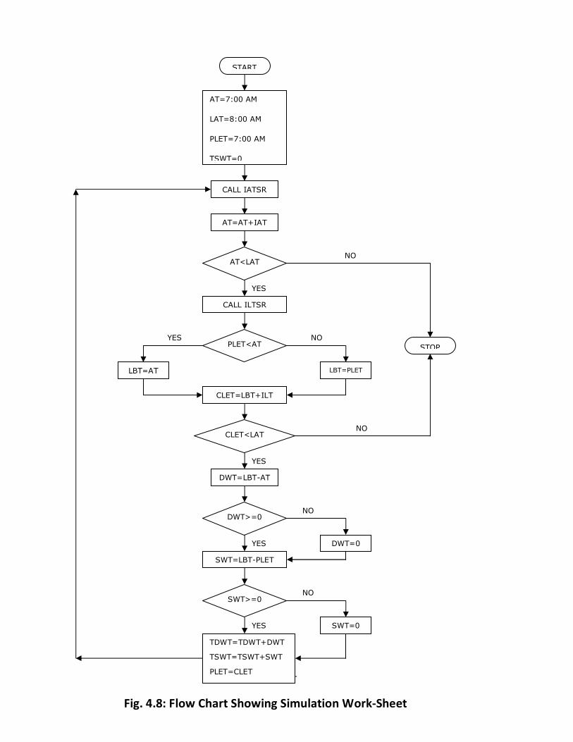
- 52 -
STOP
YES
YES
NO
NO DWT>=0
SWT=LBT-PLET
DWT=0
SWT>=0
TDWT=TDWT+DWT
TSWT=TSWT+SWT
PLET=CLET
SWT=0
YES
NO
NO YES
CLET<LAT
PLET<AT
LBT=PLET LBT=AT
CLET=LBT+ILT
NO
YES
CALL IATSR
AT=AT+IAT
AT<LAT
CALL ILTSR
AT=7:00 AM
LAT=8:00 AM
PLET=7:00 AM
TSWT=0
START
DWT=LBT-AT
Fig. 4.8: Flow Chart Showing Simulation Work-Sheet
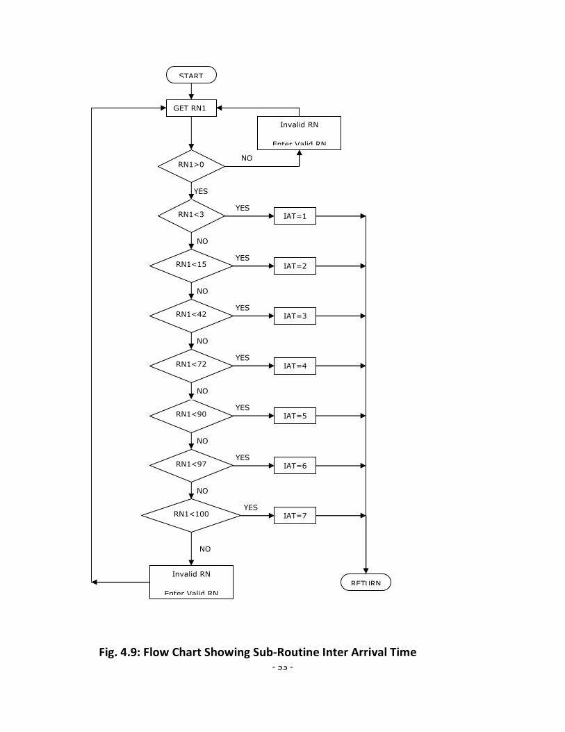
- 53 -
NO
NO
RETURN
NO
YES IAT=6
YES IAT=7
YES IAT=5 RN1<90
RN1<97
RN1<100
Invalid RN
Enter Valid RN
NO
NO
NO
NO
RN1<3 YES
IAT=1
YES IAT=2
YES IAT=3 RN1<42
YES IAT=4
RN1<15
RN1<72
YES
NO
START
GET RN1
RN1>0
Invalid RN
Enter Valid RN
Fig. 4.9: Flow Chart Showing Sub-Routine Inter Arrival Time

- 54 -
Fig. 4.10: Flow Chart Showing Sub-Routine Inter Loading Time
RETURN ILT
Invalid RN
Enter Valid RN
NO
YES ILT=6 RN1<100
NO
YES ILT=5 RN1<95
NO
NO
NO
YES ILT=3 RN1<50
YES ILT=4 RN1<80
NO
RN1<5 YES
ILT=1
YES ILT=2 RN1<20
YES
NO
START
GET RN2
RN2>0
Invalid RN
Enter Valid RN

- 55 -
4.4 RESULTS:
The following information can be obtained from the above simulation work sheet based on the
period one hour only.
a) Average Queue Length = No of dumpers in the waiting line /No. = 5/17
= 0.294
b) Average Waiting Time for the Dumper before Loading = Dumper waiting time / No of
Arrivals = 13/17 = 0.76
c) Average Loading Time = Total Loading Time/No of Arrival = 50 / 17 = 2.94 minutes
d) Time a Dumper Spend in the System = Average Loading Time + Average Waiting Time
before Loading = 2.94 + 0.76 = 3.70 minutes
4.4 CONCLUSION:
Simulation Work-Sheet developed in this problem also states that if one or more dumper
is added in the system. There is no need for a dumper to wait in the queue. But, before effecting
any decision, the cost of having an additional shovel has to compare with the cost due to dumper
waiting time. This can be worked out as follows:
Table 4.11: Cost Comparison of with one Shovel and with two Shovels
One hour period Cost with one shovel Cost with two shovels
Dumper waiting time
13 minutes * Rs 1850/- per
minutes
Rs 401/- Nil
Shovel cost Rs 4300/- Rs 8600/-
Total cost for one hour
period
Rs 4701/- Rs 8600/-
So, we see clearly that for one hour period dumper loss 13 minutes for which provide of one
additional shovel will not be a wise decision. The same way we can calculate the cost of one
additional dumper which is to be compared with time loss due shovel waiting time.

- 56 -
Table 4.12: Cost Comparison of with existing dumper and one additional dumper.
One hour period Cost with existing dumper Cost with one additional
dumper
Shovel waiting time(11
minutes *Rs 4300/-)
Rs 788/- Nil
Dumper’s cost N N + 1850/-
Total cost of one hour
period
N + 788/- N + 1850/-
Also addition of one more dumper is costlier than the no of existing dumper with shovel loss
due to waiting time. Hence the selection of equipment is optimum with this simulation work
sheet. Now, it depends on management’s philosophy that if they want to calculate maximum
loss due to shovel and dumper is manageable but at the same time the primary crusher will be
idle, and the entire transporting system will be idle, etc these will cost drastic production loss.
So, one more shovel or dumper or both are to be added in the system whichever is less though it
is not economic, but in greater sense it will help to continue the entire system and much
economical.
4.6 PERFORMANCE APPRAISAL OF MINING MACHINARIES
The 10 events which were identified from the mine data analyzed were:
Even 1 : Breakdown of shovel
Event 2 : Breakdown of Dumper,
Event 3 : Breakdown of drilling machineries,
Event 4 : Breakdown of Dozer,
Event 5 : Breakdown of Primary crusher
Event 6 : Tripping of Conveyor belt
Event 7 : General maintenance,
Event 8 : Power Failure
Event 9 : Breakdown of Narrow gauged rail transport
Event 10 : Breakdown of reclaimer
The breakdown data of all the 10 events were analyzed for a period of two years. A specific
example is shown below:

- 57 -
4.7 Specific example for data analysis
The list of following tables shows the break-down data analysis of different machineries.
Table 4.10: Frequency and period of existence of breakdown of shovel
Date Time needed in
hours
Frequency of
Shovel
Breakdown
Period of existence in hours
12.04.2009 -- --
15.04.2009 96 1 6.331
16.04.2009 24 1 15.101
29.04.2009 312 1 5.511
01.11.2009 48 1 3.887
02.11.2009 24 1 3.218
16.11.2009 336 1 0.367
17.11.2009 24 1 4.110
18.11.2009 24 1 15.650
29.11.2009 264 1 3.698
30.11.2009 24 1 2.650
17.12.2009 408 1 0.235

- 58 -
Table 4.11: Conversion of interval between shovel break-downs to cumulative
random numbers
Interval between
shovel breakdown
Frequency of
occurrence
Frequency of occurrence
% * random nos
Cumulative random
numbers
0-100 7 7000 0 - 7000
200-300 1 1000 7001-8000
300-400 2 2000 8001-10,000
400-500 1 1000 10,001-11,000
11 11,000
Table 4.12: Conversion of Existence of Shovel Breakdown to cumulative
random numbers
Existence of shovel
breakdown
Frequency of
occurrence
Frequency of
occurrence % *
random nos
Cumulative random
nos
0-1 2 2000 0-2000
2-3 1 1000 2001-3000
3-4 3 3000 3001-6000
4-5 1 1000 6001-7000
5-6 1 1000 7001-8000
6-7 1 1000 8001-9000
15-16 2 2000 9001-11,000
11 11,000

- 59 -
Table 4.13: Frequency and period of existence of breakdown of dumper
Date Time needed in
hours
Frequency Period of existence in hours
15.04.2009 72 1 0.645
16.04.2009 24 1 0.231
29.04.2009 72 1 2.331
01.11.2009 48 1 0.687
16.11.2009 360 1 6.450
17.11.2009 24 1 15.220
18.11.2009 24 1 3.335
29.11.2009 264 1 16.000
30.11.2009 24 1 5.660
17.12.2009 408 1 2.275
22.12.2010 504 1 5.020
Table 4.14: Conversion of interval between Dumper break-downs to
cumulative random numbers
Interval between
dumper breakdown
Frequency of
occurrence
Frequency of occurrence
% * random nos
Cumulative random
numbers
0-100 7 7000 0 – 7000
200-300 1 1000 7001-8000
300-400 1 1000 8001-9000
400-500 1 1000 9001-10,000
500-600 1 1000 10,001-11,000
11 11,000

- 60 -
Table 4.15: Conversion of Existence of Dumper breakdown to cumulative
random numbers
Existence of dumper
breakdown
Frequency of
occurrence
Frequency of
occurrence % *
random nos
Cumulative random
nos
0-1 3 2000 0-2000
2-3 2 1000 2001-3000
3-4 1 3000 3001-6000
5-6 1 1000 6001-7000
6-7 1 1000 7001-8000
15-16 2 1000 9001-10,000
10 10,000
Table 4.16: Conversion of interval between Drill Machine break-downs to
cumulative random numbers
Interval between drill
machine breakdown
Frequency of
occurrence
Frequency of occurrence
% * random nos
Cumulative random
numbers
0-100 7 7000 0 - 7000
200-300 2 2000 7001-9000
300-400 1 1000 9001-10,000
800-900 2 2000 10,001-12,000
12 12,000

- 61 -
Table 4.17: Frequency and period of existence of breakdown of Drill Machine
Date Time needed in
hours
Frequency Period of existence in hours
15.04.2009 72 1 6.500
16.04.2009 24 1 3.650
29.04.2009 208 1 3.554
01.11.2009 48 1 8.554
02.11.2009 24 1 2.750
16.11.2009 336 1 15.500
17.11.2009 24 1 14.550
18.11.2009 24 1 5.000
29.11.2009 264 1 1.500
30.11.2009 24 1 0.550
05.01.2010 840 2 1.250

- 62 -
Table 4.18: Conversion of Existence of Drill Machine breakdown to
cumulative random numbers
Existence of drill
machine breakdown
Frequency of
occurrence
Frequency of
occurrence % *
random nos
Cumulative random
nos
0-1 1 1000 0-1000
1-2 3 3000 1001-4000
2-3 1 1000 4001-5000
3-4 2 2000 5001-7000
5-6 1 1000 7001-8000
6-7 1 1000 8001-9000
8-9 1 1000 9001-10,000
14-15 1 1000 10001-11000
15-16 1 1000 11001-12,000
12 12,000

- 63 -
Table 4.19: Frequency and period of existence of breakdown of Dozer
Date Time needed in
hours
Frequency Period of existence in hours
15.04.2009 360 1 2.330
16.04.2009 24 1 5.011
29.04.2009 312 1 0.329
01.11.2009 48 1 1.117
02.11.2009 24 1 0.358
16.11.2009 336 1 15.116
17.11.2009 24 1 6.238
18.11.2009 24 1 4.981
29.11.2009 264 1 2.258
30.11.2009 24 1 1.661
17.12.2009 408 1 9.884
18.12.2009 12 1 3.337
Table 4.20: Conversion of interval between Dozer break-downs to cumulative
random numbers
Interval between
dozer breakdown
Frequency of
occurrence
Frequency of occurrence
% * random nos
Cumulative random
numbers
0-100 7 7000 0 - 7000
200-300 1 1000 7001-8000
300-400 3 3000 8001-11,000
400-500 1 1000 11,001-12,000
12 12,000
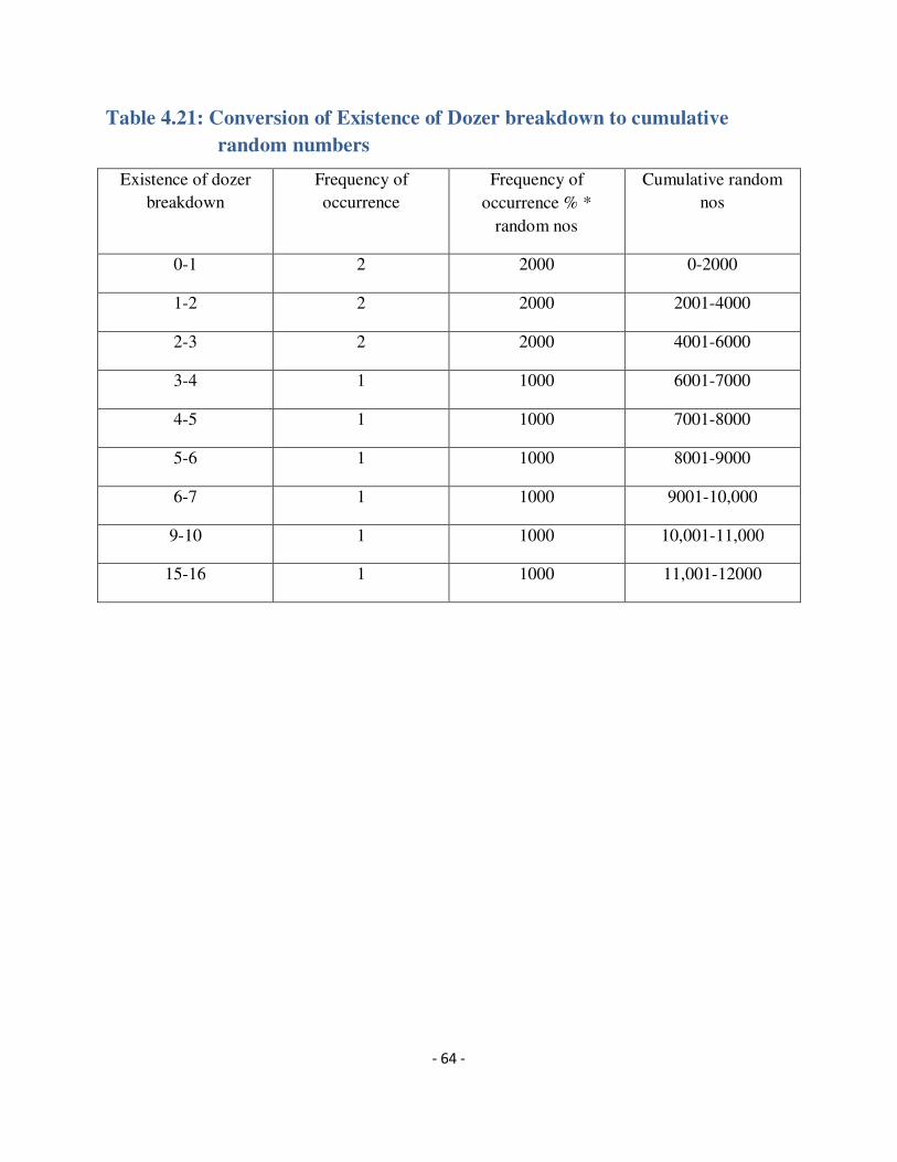
- 64 -
Table 4.21: Conversion of Existence of Dozer breakdown to cumulative
random numbers
Existence of dozer
breakdown
Frequency of
occurrence
Frequency of
occurrence % *
random nos
Cumulative random
nos
0-1 2 2000 0-2000
1-2 2 2000 2001-4000
2-3 2 2000 4001-6000
3-4 1 1000 6001-7000
4-5 1 1000 7001-8000
5-6 1 1000 8001-9000
6-7 1 1000 9001-10,000
9-10 1 1000 10,001-11,000
15-16 1 1000 11,001-12000

- 65 -
Table 4.22: Frequency and existence of breakdown of Primary Crusher
Date Time needed in
hours
Frequency Period of existence in hours
15.04.2009 336 1 2.300
16.04.2009 24 1 6.500
29.04.2009 312 1 4.201
01.11.2009 48 1 0.335
02.11.2009 24 1 11..225
16.11.2009 224 1 5.555
18.11.2009 48 1 2.228
29.11.2009 264 1 2.550
30.11.2009 24 1 0.650
17.12.2009 408 1 1.250
18.12.2009 24 1 3.650
05.03.2010 1488 1 7.500
Table 4.23: Conversion of interval between Primary Crusher break-downs to
cumulative random number
Interval between primary
crusher breakdown
Frequency of
occurrence
Frequency of occurrence % *
random nos
Cumulative random
numbers
0-100 6 6000 0 - 6000
200-300 2 2000 6001-8000
300-400 2 2000 8001-10,000
400-500 1 1000 10,001-11,000
1400-1500 1 1000 11,001-12,000
12 12,000

- 66 -
Table 4.24: Conversion of Existence of Primary Crusher breakdown to
cumulative random numbers
Existence of primary
crusher breakdown
Frequency of
occurrence
Frequency of
occurrence % *
random nos
Cumulative random
nos
0-1 2 2000 0-2000
1-2 1 1000 2001-3000
2-3 3 3000 3001-6000
3-4 1 1000 6001-7000
4-5 1 1000 7001-8000
5-6 1 1000 8001-9000
6-7 1 1000 9001-10,000
7-8 1 1000 10,001-11,000
11-12 1 1000 11,001-12,000
12 12,000
Table 4.25: Frequency and period of existence of Tripping of Belt Conveyor
Date Time needed in
hours
Frequency Period of existence in hours
15.04.2009 816 1 6.500
16.04.2009 24 1 6.225
29.04.2009 312 1 4.000
01.11.2009 4368 1 0.250
02.11.2009 24 1 1.050
16.11.2009 336 1 7.018
21.11.2009 120 1 1.257
30.11.2009 216 1 3.897
17.12.2009 408 1 4.008
18.12.2009 24 1 12.050
06.03.2010 1632 2 7.225
28.05.2010 1992 2 6.665
29.06.2010 744 1 0.254

- 67 -
Table 4.26: Conversion of interval between Belt Conveyor break-downs to
cumulative random numbers
Interval between belt
conveyor breakdown
Frequency of
occurrence
Frequency of occurrence
% * random nos
Cumulative random
numbers
0-100 3 3000 0 - 3000
100-200 1 1000 7001-8000
200-300 1 1000 8001-9000
300-400 2 2000 9001-11,000
400-500 1 1000 11,001-12,000
700-800 1 1000 12,001-13,000
800-900 1 1000 13,001-14,000
1600-1700 2 2000 14,001-16,000
1900-2000 2 2000 16,001-18,000
4300-4400 1 1000 16,001-17,000
15 15,000
Table 4.27: Frequency and period of existence of breakdown of Rail
Transport
Date Time needed in
hours
Frequency Period of existence in hours
15.04.2009 792 1 3.210
20.04.2009 120 1 2.500
29.06.2009 1680 1 6.500
01.11.2009 2880 2 12.000
06.11.2009 120 1 5.122
17.11.2009 264 1 0.365
18.11.2009 24 2 2.225
29.11.2009 264 2 4.550
17.12.2009 432 1 7.564
19.12.2009 60 1 4.124
26.03.2010 2400 2 2.550
17.04.2010 528 1 8.120
23.05.2010 864 1 0.336

- 68 -
Table 4.28: Conversion of Existence of Belt Conveyor breakdown to
cumulative random numbers
Existence of belt
conveyor breakdown
Frequency of
occurrence
Frequency of occurrence
% * random nos
Cumulative random
nos
0-1 2 2000 0-2000
1-2 2 2000 2001-4000
3-4 1 1000 4001-5000
4-5 2 2000 5001-7000
6-7 4 4000 7001-11,000
7-8 3 3000 11,001-14000
12-13 1 1000 14,001-15,000
15 15,000
Table 4.29: Conversion of interval between Rail Transport break-downs to
cumulative random numbers
Interval between rail
transport breakdown
Frequency of
occurrence
Frequency of occurrence
% * random nos
Cumulative random
numbers
0-100 3 3000 0 - 3000
100-200 2 2000 3001-5000
200-300 3 3000 5001-8000
400-500 1 1000 8001-9,000
500-600 1 1000 9,001-10,000
700-800 1 1000 10,001-11,000
800-900 1 1000 11,001-12,000
1600-1700 1 1000 12,001-13,000
2400-2500 2 2000 13,001-15,000
2800-2900 2 2000 15,000-17,000
17 17,000

- 69 -
Table 4.30: Conversion of Existence of Rail Transport breakdown to
cumulative random numbers.
Existence of rail
breakdown
Frequency of
occurrence
Frequency of
occurrence % * random
nos
Cumulative random nos
0-1 2 2000 0-2000
2-3 5 5000 2001-7000
3-4 1 1000 7001-8000
4-5 3 3000 8001-11,000
5-6 1 1000 11,001-12,000
6-7 1 1000 12,001-13,000
7-8 1 1000 13,001-14,000
8-9 1 1000 14,001-15,000
12-13 2 2000 15,001-17,000
17 17,000
Table 4.31: Frequency and period of existence of breakdown of electric sub-
station, transformer and other electric equipments
Date Time needed in hours Frequency Period of existence in hours
15.04.2009 336 2 5.010
16.04.2009 36 1 0.400
29.04.2009 312 1 1.195
02.07.2009 1488 1 1.500
02.11.2009 2880 1 2.575
16.11.2009 336 1 0.575
17.11.2009 36 1 3.362
18.11.2009 24 2 11.200
29.11.2009 264 1 2.500
30.11.2009 36 1 8.597
17.12.2009 408 1 2.528
18.12.2009 24 1 4.414
05.01.2010 432 1 5.000
06.1.2010 24 2 6.321
08.02.2010 48 2 1.255
10.02.2010 60 1 2.125
19.02.2010 216 1 5.589
25.03.2010 816 1 9.994
30.03.2010 120 1 3.556
30.04.2010 744 1 0.255
29.05.2010 696 2 11.255

- 70 -
Table 4.32: Conversion of interval between Belt Conveyor break-downs to
cumulative random numbers
Interval between belt
conveyor breakdown
Frequency of
occurrence
Frequency of occurrence
% * random nos
Cumulative random
numbers
0-100 11 11000 0 - 11000
100-200 1 1000 11,001-12,000
200-300 2 2000 12,001-14,000
300-400 4 4000 14,001-18,000
400-500 2 2000 18,001-20,000
600-700 2 2000 20,001-22,000
700-800 1 1000 22,001-23,000
800-900 1 1000 23,001-24,000
1400-1500 1 1000 24,001-25,000
2800-2900 1 1000 25,001-26,000
26 26,000
Table 4.33: Conversion of Existence of electric sub-station etc. Break down to
cumulative random numbers
Existence of shovel
breakdown
Frequency of
occurrence
Frequency of
occurrence % *
random nos
Cumulative random
nos
0-1 3 3000 0-3000
1-2 4 4000 3001-7000
2-3 4 4000 7001-11,000
3-4 2 2000 10,001-13,000
4-5 1 1000 13,001-14,000
5-6 4 4000 14,001-18,000
6-7 2 2000 18,001-20,000
8-9 1 1000 20,001-21,000
9-10 1 1000 21,001-22,000
11-12 4 4000 22,001-26,000
26 26,000

- 71 -
Table 4.34: Frequency and period of existence for General Maintenance
Date Time needed in
hours
Frequency Period of existence in hours
16.04.2009 816 1 1.230
29.04.2009 72 1 0.891
01.08.2009 2116 1 5.559
02.11.2009 2208 2 0.423
16.11.2009 336 2 3.544
17.11.2009 24 1 3.801
18.11.2009 36 1 0.654
17.12.2009 720 1 4.220
18.12.2009 36 1 7.110
05.01.2010 432 1 5.558
06.01.2010 24 1 2.000
14.02.2010 912 2 1.141
26.02.2010 288 1 0.631
03.03.2010 168 1 7.554
04.03.2010 36 1 2.910
13.03.2010 216 1 11.250
25.03.2010 300 1 9.119
26.03.2010 24 2 8.429
22
Table 4.35: Conversion of interval between General Maintenances to
cumulative random numbers
Interval between
general maintenances
Frequency of
occurrence
Frequency of occurrence
% * random nos
Cumulative random
numbers
0-100 8 8000 0 - 8000
100-200 1 1000 8001-9000
200-300 2 2000 9001-11,000
300-400 3 3000 11,001-14,000
400-500 1 1000 14,001-15,000
700-800 1 1000 15,001-16,000
800-900 1 1000 16,001-17,000
900-1000 2 2000 17,001-19,000
2100-2200 1 1000 19,001-20,000
2200-2300 2 2000 20,001-22,000
22 22,000

- 72 -
Table 4.36: Conversion of Existence for General Maintenance to cumulative
random numbers
Existence of general
maintenance
Frequency of
occurrence
Frequency of occurrence
% * random nos
Cumulative random
nos
0-1 4 4000 0-4000
1-2 3 3000 4001-7000
2-3 2 2000 7001-9,000
3-4 3 3000 9,000-12,000
4-5 2 2000 12,001-14,000
5-6 2 2000 14,001-16,000
7-8 2 2000 16,000-18,000
8-9 2 2000 18,001-20,000
9-10 1 1000 20,000-21,000
11-12 1 1000 21,001-22,000
22 22,000
Table 4.37: Frequency and period of existence of Reclaimer Break-down
Date Time needed in
hours
Frequency Period of existence in hours
06.04.2009 600 1 1.230
29.04.2009 552 1 0.891
01.08.2009 2116 1 5.559
02.09.2009 744 2 0.423
06.11.2009 1536 2 3.544
17.11.2009 264 1 3.801
18.11.2009 36 1 0.654
17.12.2009 720 1 4.220
18.12.2009 24 1 7.110
05.01.2010 432 1 5.558
06.01.2010 36 1 2.000
14.02.2010 912 2 1.141
28.02.2010 336 1 0.631
03.03.2010 144 1 7.554
04.03.2010 36 1 2.910
13.03.2010 216 1 11.250
26.03.2010 312 1 9.119
26.04.2010 742 2 8.429

- 73 -
Table 4.38: Conversion of interval between reclaimer breakdown to
cumulative random numbers
Interval between
reclaimer break down
Frequency of
occurrence
Frequency of occurrence
% * random nos
Cumulative random
numbers
0-100 4 4000 0 - 4000
100-200 1 1000 4001-5000
200-300 2 2000 5001-7,000
300-400 2 2000 7001-9000
400-500 1 1000 9001-10,000
500-600 1 1000 10,000-11,000
600-700 1 1000 11,001-12,000
700-800 5 5000 12,001-17,000
900-1000 2 2000 17,001-19,000
1500-1600 2 2000 19,001-21,000
2100-2200 1 1000 21,001-22,000
22 22,000
Table 4.39: Conversion of Existence for breakdown of Reclaimer to
cumulative random numbers
Existence of reclaimer
break down
Frequency of
occurrence
Frequency of occurrence
% * random nos
Cumulative random
nos
0-1 5 5000 0-5000
1-2 3 3000 5001-8000
2-3 2 2000 8001-10,000
3-4 3 3000 10,001-13,000
4-5 1 1000 13,001-14,000
5-6 2 2000 14,001-16,000
7-8 2 2000 16,001-18,000
8-9 2 2000 18,001-20,000
9-10 1 1000 20,001-21,000
11-12 1 1000 21,001-22,000
22 22,000

- 74 -
Table 4.40: Different Events of Break-downs, their frequencies, and random-
number distribution.
Sl No Different Events of
Breakdown
Total frequency
of Breakdown
Frequency of
breakdown in %
Random Number
Distriution
1 Breakdown of
Shovel
11 6.875 6875
2 Breakdown of
Dumper
10 6.250 6250
3 Breakdown of Drill
Machine
12 7.500 7500
4 Breakdown of Dozer 12 7.500 7500
5 Breakdown of
Primary Crusher
12 7.500 7500
6 Tripping of Belt
Conveyor
15 9.375 9375
7 Breakdown of
Narrow Gauge Rail
Transport
17 10.625 10625
8 Power Failure 26 16.250 16250
9 General Maintenance 23 14.375 14375
10 Breakdown of
Reclaimer
22 13.750 13750
160 100 1,00,000
From the above mentioned analysis it is observed that the random number distribution can give
some indication about the occurrences of the break-down of different events like;
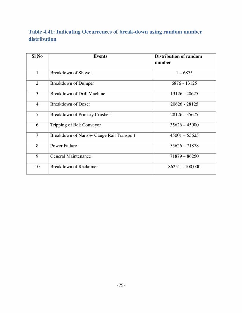
- 75 -
Table 4.41: Indicating Occurrences of break-down using random number
distribution
Sl No Events Distribution of random
number
1 Breakdown of Shovel 1 – 6875
2 Breakdown of Dumper 6876 - 13125
3 Breakdown of Drill Machine 13126 - 20625
4 Breakdown of Dozer 20626 - 28125
5 Breakdown of Primary Crusher 28126 - 35625
6 Tripping of Belt Conveyor 35626 – 45000
7 Breakdown of Narrow Gauge Rail Transport 45001 – 55625
8 Power Failure 55626 – 71878
9 General Maintenance 71879 – 86250
10 Breakdown of Reclaimer 86251 – 100,000

- 76 -
PROGRAMMING FOR RANDOM NUMBER OF DIFFERENT EVENTS
# include<iostrem.h>
# include<conio.h>
# include<stdlib.h>
# include<time.h>
Int UNRAND ();
Int_EVENTS_IDENTIFICATION ();
Void main ()
{
clscr ();
Int R;
Randomized ();
R = random (100000);
cout<<”Uniform Random Number R =”<<R<</n”
cout <<”For this R The Event Generated is :/n”;
If (R<6876)
cout <<”Event -1: Break-down of Shovel”;
else if (R>=6876 && R<13126)
cout <<”Event -2: Break-down of Dumper”;
else if (R>=13126 && R<20126)
cout <<”Event -3: Break-down of Drill Machine”;
else if (R>=20626 && R<28126)
Cout <<”Event -4: Break-down of Dozer”;

- 77 -
else if (R>=28126 && R<35626)
cout <<”Event -5: Break-down of Primary Crusher”;
else if (R>=35626 && R<45001)
cout <<”Event -6: Tripping of Belt Conveyor”;
else if (R>=45001 && R<55626)
cout <<”Event -7: Break-down of Narrow Gauge Rail Transport”;
else if (R>=55226 && R<71878)
cout <<”Event -8: Power Failure”;
else if (R>=71879 && R<86250)
cout <<”Event -9: General Maintenance”;
else if (R>=86251 && R<100000)
cout <<”Event -10: Break-down of Dumper”;
getch ()
}

- 78 -
Chapter 5
SUMMARY AND CONCLUSION
Production scheduling along with production planning, provides projections of future
mining progress and time requirements for the development and extraction of a resource. These
schedules and plans are used by management as means of attaining the following objections;-
(1) Maintaining or maximizing expected profit,
(2) Determining future investment in mining,
(3) Optimizing return on investment, (ROI)
(4) Evaluating alternative investments, and
(5) Conserving and developing owned resourced.
The first four goals are generally concerned with mining cost, both capital and operation
requirements, and as such, play an important role a production planning. However, this chapter is
concerned with the fifth management objective of resource development in order to conserve and
perpetuate the corporate entity. The following discussion is based on the premise that detailed
economic evaluations and market surveys have been performed and analyzed and that the results
indicate a viable projects.
Simulation Work-Sheet developed in this problem also states that if one or more dumper
is added in the system. There is no need for a dumper to wait in the queue. But, before effecting
any decision, the cost of having an additional shovel has to compare with the cost due to dumper
waiting time. This can be worked out in reference to table no 4.11 and 4.12.
The breakdown of different machineries is analyzed with random number distribution.
The different event falls under definite random number distribution range. Such as if random
number comes as 1 - 6875 indicates the shovel breakdown and if it comes 6876- 13125 it will be
considered as dumper break-down, etc. Hence a clear idea can be made for the break-down of
different machineries also precautions can be taken for preventive maintenance to minimize
these break-down periods by analyzing this method and thus production can be set as Optimum
and steady-state.

- 79 -
REFERENCES
1. Deo, Narsingh, (1979) System simulation with digital computer, Prentice Hall India,
2. Wilke F. L., Mueller K. and Wright E. A. (1984), Ultimate Pit and Production Scheduling
Optimization, Proceedings of 18th
International Symposium on Application of computer and
Operating Research in the Mineral Industry, London 26th – 30
th March, London: The
Institution of Mining and Metallurgy, First Edition, pp. 29-38.
3. Ramajon, S. and Dimitrakopoulos, R. (2003), Production Scheduling Optimization in a
Nickle Laterite Deposite; MIP and LP Application and Infeasibility in the Presence Ore Body
Variability, Proceedings of the 12th International Symposium on Mine Planning and
Equipment Selection, Kalgoorlie, 23rd
– 25th
April, Kuruppu, M. D. and Lilly, P.A. (Eds),
Carlton: Australian Institute of Mining and Metallurgy, pp. 1-5.
4. Ramajon, S. and Dimitrakopoulos, R. (2004), Traditional and New MIP Models for
Production Scheduling with In-Situ Grade Variability, International Journal of Mining
Reclamation and Environment, Vol. 18, No. 2, pp. 85-98.
5. Ramajon, S. and Dimitrkopoulos, R. (2007), Stochastic Optimization of Long Term
Production Scheduling for Open Pit Mines With a New Integer Programming Formulation,
Ore Body Modelling and Strategic Mine Planning, Dimitrakopolous, R. (Ed), Carlton:
Australasian Institute of Mining and Metallurgy, Spectrum Series, Vol. 14, First Edition, pp.
353-360.
6. Praehofer, H., (1991) “System Theoretic Foundation of Combined Discrete Continued
System Simulation”, Doctoral dissertations Johannes Kepler University of Ling, Ling,
Austria.
7. Seong, M. Cho, and T. G. Kin, (1998) “Real-Time DEVS Simulation: Concurrent, Time-
Selective Execution Combined RT-DEVS Model and Interactive Environment”, Proceedings
of SCSC-98, July 19-22, 1998, Reno, NV, PP. 410-415.
8. Takahashi, S., and Y. Takahara, (1995) Logical Approach of System Theory. Springer-
Verlag, London, 1995.
9. Wymore, A. W., (1993) Model-Based Systems Engineering: An Introduction to the
Mathematical Theory of Discrete System and to the Tricotyledon Theory of System Design.
CRC Press, 1993.
10. Zeigler, B. P., and J. S. Lee. (1998) Theory of Quantized Systems: Formal Basis for
DEVS/HLA Distributed Simulation Environment. Enabling Technology for Simulation (II),
SPIE Aeorosense 98. Orlando, FL, 1998.
11. Arik, A. (1999), An Alternative Approach Research Resourece Classification Proceedings
of 28th International Symposium on Application of Computer Method in the Mineral

- 80 -
Industry, Golden, Colorado, 20th-22
nd October, Dagdelen K., Dardano C., Fransisco M. and
Proud J. (Eds.), Golden: Colorado Scool of Mines, First Edition, pp. 45-53.
12. Bagchi, T. P. (1999), Multi Objective Scheduling by Genetic Algorithm, Boston: Kluwer
Academic, First Edition.
13. Caers, J. (2000), Adding Local Accuracy to direct sequential Simulation, Mathematical
Geology, Vol. 32, No. 7, pp. 815-850.
14. Chakraborty, N., Sreevathsan, R., Jayakanth, R., Bhattacharya, B. (2009), Tailor-Made
Material Design: An Evalutionary Approach Using Multi Objective Genetic Algorithms,
Computational Materials Science, Vol. 45, No. 1, pp. 1-7.
15. Dagdelen, K. (2005), Open Pit Optimization- Strategic for Improving Economic Mine
Planning, Ore Body Modelling and Strategic Mine Planning – Uncertainity and Risk
Management Model, Dimitrakopoulos, R. (Eds.), Karlton Victoria: Australasian Institute of
Mining Metallurgy, Spectrum series, Vol. 14, pp. 125-128.
16. Denbi, B. and Schofild, D. (1994), Open pit Design and Scheduling by use of Genetic
Algorithms, Transaction of Institute of Mining and Metallurgy, Section A, Vol. 103, pp. A
221- A 226.
17. Dimitrakopoulos, R. (1998), Conditional Simulation Algorithms for Modeling Ore Body
Uncertainty in Open Pit Optimization, International Journal of Mining, Reclamation and
Environment, Vol. 12, No. 4 pp. 193-197.
18. Dimitrakopoulos, R. and Ramajon, S. (2004), Uncertainty Based Production Scheduling in
Open Pit Mining, Society of Mining and Metallurgy, and Exploration Transaction, Vol.316,
pp. 106-112.
19. Dowd, P. A. (1994), Risk Assessment in Reserve Estimation and Open Pit Planning.
Transaction of Institute of Mining and Metallurgy, Section A, Vol. 103, pp. A 148 - A154.
20. Dowd, P. and Onur, A. (1992), Optimizing Open Pit Design and Sequence, Proceedings of
30th International Symposium on Application of Computer and Operation Research in the
Mineral Industry, Tucson, Arizona, 7th
-11th
April, Kim Y. C. (Ed.), Littleton: Society for
Mining, Metallurgy, and Exploration, First Edition, pp. 411-422.
21. Radhakrishnan, V. R. and Sen, P., (1982), Optimum nos of Storage Bins for Off-
Specification products by Mote-Carlo Simulation, Indian Chemical Engineer, pp. 16 – 23.
22. Sentiappan, R. and Roy, S. C. (1983) Application of Queuing Theory in Open pit Equipment
Selection, Tr. Mining, Geology, Metallurgy, Inst. India, pp. 80-92.
23. Pal, B. K., (1984). Simulation of the Rapid Loading System of an Iron Ore Processing Plant,
M.Tech. Thesis I.I.T. Kharagpur.

- 81 -
24. Hausner Bemard, Harry, M. Marcowitz, Herbert, W. Karr, (1963) Simscript a Simulation
Programming Language, Prentice Hall, India. pp. 56-72.
25. Hammersly, J. M. and Handcomb, D. C. (1964) Monte-Carlo Methods, Jhon Wiley and Sons,
Newyork, pp. 23-29.
26. Brahma, K. C., Pal, B. K. and Das, C. (2004): Study on Application of Petri Nets in Opencast
Mining, 13th
Int. Symp. on Mine Planning and Equipment Selection (MPES–2004),
September 01-04, , held in Wroclaw, Poland, edited by A. A. Balkema, Rotterdam, pp. 01 --
06.
27. Dey, K. and Pal, B. K. (2008): Ground Vibration – Unique Case Studies in Open Cast Mines,
6th
Int. Conf. Case Histories in Geotechnical Engineering. Aug. 11--16, 2008, held in Univ.
of Missouri, Rolla, USA, pp. 327 – 338.
28. Dowd, P. and Onur, A. (1992): Optimizing Open Pit Design and Sequence, Proceedings of
30th Int. Symp. on Application of Computer and Operation Research in the Mineral Industry,
Tucson, Arizona, 7th -11
th April, Kim Y. C. (Ed.), Littleton: Society for Mining, Metallurgy,
and Exploration, First Edition, pp. 411-422.
29. Ghosh, A. K. (2004): Mine Equipment Selection using Failure Mode and Effects and
Criticality Analysis, 13th
Int. Symp. on Mine Planning and Equipment Selection (MPES–
2004), September 01-04, , held in Wroclaw, Poland, edited by A. A. Balkema, Rotterdam,
pp. 449 -- 454.
30. Jayanthu, S. (2011): Ground Vibrations Generated by Blasting, Nat. Sem. on Explosives and
Blasting Techniques for Mining, Quarrying & Infrastructure Industry (EBTMQI), Feb. 18-
19, 2011, held at KNIT, Surathkal, pp. 116-127.
31. Naik, H.K. and Patnaik, N.K. (1993): Application of Auto-CAD for Design and Planning of
Dragline Mines, Indian Conf. on Computer applications in mineral Industry, held in Chennai,
Tamilnadu, India, pp. 81-92.
32. Pal, B. K. (1994): Simulation Technique for the Performance Appraisal of Open-pit Mine
Machinery, Proc. of the 3rd
Int. Symp. on the Mine Planning and Equipment Selection, Oct.
18-20, 1994, held at Istanbul, Turkey, edited by A. A. Balkema, Rotterdam, pp. 501-507.
33. Ramajon, S. and Dimitrkopoulos, R. (2007): Stochastic Optimization of Long Term
Production Scheduling for Open Pit Mines With a New Integer Programming Formulation,
Ore Body Modeling and Strategic Mine Planning, Dimitrakopolous, R. (Ed), Carlton:
Australasian Institute of Mining and Metallurgy, Spectrum Series, Vol. 14, First Ed. , pp.
353-360.
34. Samanta B, Kumar A, Bhattacherjee A, and Chatterjee S, (2007): Open Pit Mine design in
Presence of Uncertainty Due to Ore Grade Modeling, Mineral Resource Engineering, Vol.
12, No. 4, P 241-257.

- 82 -
35. Snehamoy Chatterjee, Amina Lamghari and Roussos Dimitrakopoulos A. (2010): Two-Phase
Heuristic Method for Constrained Pushback Design, Proceeding of the 4th
Int. Conf. on
Mining Innovation (MININ2010) Raul Castro, Xavier Emery, and Romke Kuyvenhoven
(Ed.), Santiago, Chile, June, 2010.
36. Gershon, M. E. (1987), Heuristic Approaches for Mine Planning and Production Scheduling,
International Journal of Mining and Geological Engineering, Vol. 5, pp. 1-13.
37. Kumral, M. and Dowd, P.A. (2002), Short-term Mine Production Scheduling for industrial
Minerals using Multi-objective Simulated Annealing, Proceedings of 30th International
Symposium on Application of Computers and Operations Research in the Mineral Industry,
Phoenix, 25th
-27th
February, Bandopadhyay, S. (Ed.), Littleton: The Society of Mining,
Metallurgy and Exploration, First Edition, pp. 13-19.

- 83 -
Appendix-A
Fig A. 1 (A) Break-down analysis of shovel
Fig A. 1 (B) Break-down analysis of shovel
0
5
10
15
20
25
30
1 2 3 4 5 6 7 8 9 10 11 12 13 14 15 16
Fre
qu
en
cy in
%
Duration of Breakdown period hours
(A) Break-down Analysis of Shovel
0
10
20
30
40
50
60
70
1 2 3 4 5
Fre
qu
en
cy in
%
Time interval of Break-downs, (*100 hours)
(B) Break-down of Shovel Analysis

- 84 -
Fig A. 2 (A) Break-down analysis of Dumper
Fig A. 2 (B) Break-down analysis of Dumper
0
0.5
1
1.5
2
2.5
3
3.5
1 2 3 4 5 6 7 8 9 10 11 12 13 14 15 16 17 18
Fre
qu
en
cy in
%
Durationof break-down period (hours)
(A) Break-down analysis of Dumper
0
10
20
30
40
50
60
70
1 2 3 4 5
Fre
qu
en
cy in
%
Time Interval of Break-downs (*100 hours)
(B) Breakdown of Dumper analysis

- 85 -
Fig A. 3 (A) Break-down analysis of Drill Machine
Fig A. 3 (B) Break-down analysis of Drill Machine
0
0.5
1
1.5
2
2.5
3
3.5
1 2 3 4 5 6 7 8 9 10 11 12 13 14 15 16 17 18
Fre
qu
en
cy in
%
Duration of break-down period (*100 hours)
(A) Break-down analysis of Drill
Machine
0
10
20
30
40
50
60
70
1 2 3 4 5 6 7 8 9
Fre
qu
en
cy in
%
Break-down period (*100 hours)
(B) Break-down analysis of Drill
Machine

- 86 -
Fig A.4 (A) Break-down analysis of Dozer
Fig A.4 (B) Break-down analysis of Dozer
0
0.5
1
1.5
2
2.5
1 2 3 4 5 6 7 8 9 10 11 12 13 14 15 16 17
Fre
qu
en
cy in
%
Duration of Break-down period (hours)
(A) Break-down analysis of Dozer
0
10
20
30
40
50
60
70
1 2 3 4 5 6
Fre
qu
en
cy in
%
Break-down period in (*100 hours)
(B) Breakdown analysis of Dozer

- 87 -
Fig A.5 (A) Break-down analysis of Primary Crusher
Fig A.5 (B) Break-down analysis of Primary Crusher
0
0.5
1
1.5
2
2.5
3
3.5
1 2 3 4 5 6 7 8 9 10 11 12 13
Fre
qu
en
cy in
%
Break-down period in hours
(A) Break-down analysis of Primary
Crusher
0
10
20
30
40
50
60
1 2 3 4 5 6 7 8 9 10 11 12 13 14 15 16
Fre
qu
en
cy in
%
Break-down period in hours
(B) Break-down analysis of Primary
Crusher
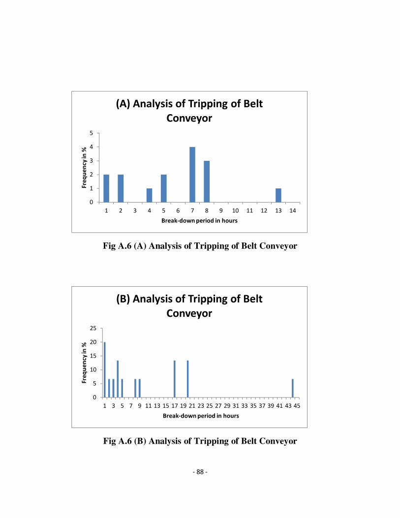
- 88 -
Fig A.6 (A) Analysis of Tripping of Belt Conveyor
Fig A.6 (B) Analysis of Tripping of Belt Conveyor
0
1
2
3
4
5
1 2 3 4 5 6 7 8 9 10 11 12 13 14
Fre
qu
en
cy in
%
Break-down period in hours
(A) Analysis of Tripping of Belt
Conveyor
0
5
10
15
20
25
1 3 5 7 9 11 13 15 17 19 21 23 25 27 29 31 33 35 37 39 41 43 45
Fre
qu
en
cy in
%
Break-down period in hours
(B) Analysis of Tripping of Belt
Conveyor

- 89 -
Fig A.7 (A) Break-down analysis of Narrow-Gauge Rail Transport
Fig A.7 (B) Break-down analysis of Narrow-Gauge Rail Transport
0
1
2
3
4
5
6
1 2 3 4 5 6 7 8 9 10 11 12 13
Fre
qu
en
cy in
%
Break-down period in hours
(A) Break-down of Narrow-Gauge Rail
Transport
0
2
4
6
8
10
12
14
16
18
20
1 3 5 7 9 11 13 15 17 19 21 23 25 27 29
Fre
qu
en
cy in
%
Break-down period in (100*hours)
(B) Break-down of Rail Transport

- 90 -
Fig A.8 (A) Analysis of Power Failure
Fig A.8 (B) Analysis of Power Failure
0
0.5
1
1.5
2
2.5
3
3.5
4
4.5
1 2 3 4 5 6 7 8 9 10 11 12 13
Fre
qu
en
cy in
%
Break-down period in hours
(A) Analysis of Power Failure
0
5
10
15
20
25
30
35
40
45
1 3 5 7 9 11 13 15 17 19 21 23 25 27 29
Fre
qu
en
cy in
%
break-down period in hours
(B) Analysis of Power Failure

- 91 -
Fig A.9 (A) Analysis of General Maintenance
Fig A.9 (B) Analysis of General Maintenance
0
0.5
1
1.5
2
2.5
3
3.5
4
4.5
1 2 3 4 5 6 7 8 9 10 11 12 13
Fre
qu
en
cy in
%
Break-down period in hours
(A) Analysis of General Maintenance
0
5
10
15
20
25
30
35
40
1 2 3 4 5 6 7 8 9 10 11 12 13 14 15 16 17 18 19 20 21 22 23 24
Fre
qu
en
cy in
%
Break-down period in (hours*100)
(B) Analysis of General Maintenance

- 92 -
Fig A.10 (A) Break-down analysis of Reclaimer
Fig A.10 (B) Break-down analysis of Reclaimer
0
1
2
3
4
5
6
1 2 3 4 5 6 7 8 9 10 11 12 13 14
Fre
qu
en
cy in
%
Break-down period in hours
(A) Analysis of break-down of
Reclaimer
0
5
10
15
20
25
1 2 3 4 5 6 7 8 9 10 11 12 13 14 15 16 17 18 19 20 21 22 23
Fre
qu
en
cy in
%
Break-down period in (hours*100)
(B) Analysis of break-down of
Reclaimer

- 93 -
Flag this message
Re: PAPER
Thursday, 21 April, 2011 10:44 AM From:
This sender is DomainKeys verified
"pradip chanda" <[email protected]>
Add sender to Contacts
To:
"drbk Pal" <[email protected]>
Dear Dr Pal,
Thank you for your e-mail and the paper titled "Use of Monte Carlo technique for production optimisation
from large opencast mines - a case study". The paper has been accepted for publication in a forthcoming issue
of the Journal of Mines, Metals & Fuels. However, I will let you know later in which issue this would be
published on priority basis.
With warm regards,
P K Chanda
Executive Editor
JOURNAL OF MINES, METALS & FUELS
6/2 Madan Street
Kolkata 700 072
tel: 033 22126526
fax: 033 22126348
--- On Wed, 20/1/11, drbk Pal <[email protected]> wrote:
From: drbk Pal <[email protected]>
Subject: PAPER
Date: Wednesday, 20 January, 2011, 20:47
Dear Mr. Chanda,
My greetings to you from NIT, Rourkela. Enclosed please find the Full Manuscript of our Paper entitled "Use
of Monte Carlo Technique for production Optimisation from Large Opencast Mines -- Case Study". Kindly
acknowledge teh Receipt for the same.
With best wishes and regards,
DR. PAL
DR.B.K.PAL, PROFESSOR, DEPT. OF MINING ENGINEERING,
NATIONAL INSTITUTE OF TECHNOLOGY, ROURKELA -- 769 008, INDIA.
PH. No.: +91-661-2462605/2463605; FAX:+91-661-2462999/2472926

- 94 -
USE OF MONTE-CARLO TECHNIQUE FOR PRODUCTION
OPTIMISATION FROM LARGE OPENCAST MINES - CASE STUDY
Dr. B. K. Pal
Professor, Department of Mining Engineering, National Institute of Technology,
Rourkela--769008 (Orissa), India, e-mail:[email protected]/[email protected]
and
Uttam Ghorai
Research Student, Department of Mining Engineering, National Institute of Technology,
Rourkela--769008 (Orissa), India, e-mail:[email protected]
ABSTRACT
Globally the mineral sector is going through a technological revolution to cope with the downstream
innovation. The advancement in technology has resulted in excavation of large volumes of natural resources from the mines. Mining industry is constantly search of higher levels of production with
increased productivity and reduced cost. Besides the economics operating scale, the new dimension of
development focused on automation, cleaner mining system, and increased utilization of assets by increasing machine performance. In this paper the probability of service (loading) facility of a shovel and
arrival of a dumper are individually analyzed from their previous performances and then simulated on a
simulation work-sheet using Monte-Carlo simulation technique and then computerized models are developed for optimization of production from a shovel-dumper combination in a large open-cast mines.
The entire study was done in OCL Langibarna Limestone mines in Orissa.
INTRODUCTION
Globally the mineral sector is going through a technological revolution to cope with the downstream
innovation. The advancement in technology has resulted in excavation of large volumes of natural
resources from the mines. Mining industry is constantly search of higher levels of production with
increased productivity and reduced cost. Besides the economics operating scale, the new dimension of

- 95 -
development focused on automation, cleaner mining system, and increased utilization of assets by
increasing machine performance [3].
After a mining company has got the lease of a mineral deposit the problem is then how to mine
and process that deposit the best way. The principle problem is facing managers or engineers who must
decide on mine plant size, equipment selection and long-range scheduling is how one can optimize a
properly not only intense of efficiency but also as to project duration. For faster rate of production,
mechanization at high degree is obvious. However, the charge of explosives plays an important role. The
excess charge can create ground vibration, leading to damages to structures [5].
These machineries are very costly. So, unless they are properly matched reduction in production
cost is very difficult. Increase in idle times of machineries leads to increase in production cost. In order to
reduce the idle time or waiting time the number of machineries may be increased. Due to higher cost of
machineries more investment is needed which ultimately contribute in higher production cost. So, unless
you getting perfect matching optimum numbers of equipments reduction in production cost is impossible
[1]. So, it is needed to analyze the operation of equipments considering their breakdown periods,
repairing, maintenance, and preventive maintenance, availability of spare-parts, efficiency of operators
and management philosophy etc. This study is based on use Monte-Carlo technique operation of shovel-
dumper combination.
USE OF MONTE-CARLO TECHNIQUE FOR PRODUCTION OPTIMISATION FROM LARGE
OPENCAST MINES
Many researchers have taken attempt to simulate the production optimization. Using of different
mathematical models for mine production scheduling is extensively surveyed. The introduction of the
concept of linear programming for optimization of mine production scheduling was made [9, 10]. They
used linear programming to determine a feasible extraction sequence which ultimately maximized the
total profits over the planning horizon. A dynamic cut-off grade strategy was applied to determinate
between ore and waste in a mineral deposit and this cut-off change with time. The scheduling problem
was formulated as a large scale linear programming problem considering governing constraints of the
system and further by applying decomposition principle, the problem was decomposed into simple linear
programming problem, called the master problem and set of sub-problem was relatively simple. The
drilling operation in an opencast mine with double rod drilling provision has been considered for analysis
and has been simulated [2]. Computer techniques were applied for design of dragline operation and its
graphic representation for quick processing of databases was developed [6].
Also by using
the first module of optimization calculations and construction of contours of mining operations in package
regime we receive the most priority directions of moving of mining operations by working levels. It
allows substantially decreasing time of a search of optimal contours of mining operations up to the end of
planned period [4].
- 96 -
The second
module is used for taking final decision in interactive regime and allows more adequate taking into
account possible complex situations. It may be used in addition to operations of the first module or as
independent apparatus for current and timely planning of mining operations [8].
For taking correct decision it is important to ensure a forenamed subsystems with reliable information
about interaction of parameters and indexes of operation of opencast in different mining-technical and
technological conditions with the help of spatial recognizing algorithm and formulae [7].
DESCRIPTION OF THE CASE STUDY MINES AND MACHINARIES
The OCL
Langibarna Limestone mines is fully mechanized and located at northern Orissa, 10 km away from
Rajgangpur town. The captive cement plant is at the same place. Here the massive limestone deposit is of
anticline of “Gangpur Series”. The mine is divided into six nos of different pits, marked as Pit No. -1, Pit
No. -2,…..Pit No. -6. The bench height of the mines is around 10 m and ore is to waste ratio is 1:1. The
targeted production is 10000 MT per day but due to some constraints present production is 6000-7000
MT per day. The machineries used in the mines are Drill machine: model ROCL-6 Make Atlas Cop co;
Dozer: Model D 155, 320 HP, Make Komatsu; Road grader; BEML Haul pack Dumper: of 35 MT & 50
MT; Hydraulic shovels: of 4.5 cu m. & 6.5 cu m. of bucket capacity, Make TATA Hitachi, Model PC
1250; Road Roller:10 MT; Explosive Van: 8 MT capacity; Fuel Tanker: 10 KL; water sprinkler 10KL,
18KL and 22KL; Primary crushers: 400 TPH and 1600 TPH, of L&T make; Stalker cum reclaimer: 1200
TPH of China make; Belt conveyor: Transporting from crusher to cement plant around 10 km long; Also
Narrow Gauge Loco: Transport from crusher to cement plant etc.
USE OF MONTE CARLO SIMULATION TECHNIQUE IN PRODUCTION OPTIMISATION
Simulation is a numerical technique for conducting experiments that involves certain types of
mathematical and logical relationship necessary to describe the behavior and structure of a complex real
world system over extended period of time. From definition it is the process of designing a model of a
real system and conducting experiments with this model for the purpose of understanding the behavior
(within the limit imposed by a criterion or a set of criteria) for the operation of the system. [7]. Using the
simulation we can introduce the constants and variables related to the problem, set up the possible courses
action and establish criteria which act as measures of effectiveness. The probability of service (loading)
facility of a shovel and arrival of a dumper are individually analyzed from their previous performances
and then simulated on a simulation work-sheet using Monte-Carlo simulation technique and then
computerized models are developed for optimization of production from a shovel-dumper combination in
a large open-cast mine. The entire study was done in OCL Langibarna Limestone mines in Orissa.
Table 1: Specification for Operating Cost of Shovel and Dumper

- 97 -
Model/make of machine TATA HITACHI Hydraulic Shovel BEML Dumper
Model PC - 1250 Haulpak
Bucket capacity 6.5 cu m 50 MT
Cost of the machine 2.5 crore 1.25 crore
Life of the machine 8 years 8 years
e) Depreciation cost Avg. 12% each year Avg. 12% each year
f) Fuel cost 75 lits per hour 30 lits per hour
g) Maintenance & spare parts 20% of depreciation cost 20% of depreciation cost
h) Operators & helpers wages Rs. 100/- per hour (say) Rs. 50/- per hour (say)
Effective working hours in 2 shifts
per day
10 hours per day 10 hours per day
Working days in a year 300 days 300 days
CALCULATION OF OPERATING COST OF SHOVEL:
Depreciation cost = 12% (of investment cost = 1.75 crore) Avg. per year = 2.5 * 0.12 = Rs. 30.00 lakh
per year i.e. 3000000/300 = Rs. 10000 per day = Rs. 1000/- per hour.
Fuel cost (HSD Oil) 75 liters per hour @ Rs. 40/- per lit. = Rs 3000/- per hour.
Maintenance & spare parts cost = 20% of depreciation cost = Rs. 200/- per hour.
Operators & helpers wages = Rs. 100/- (Approx.) per hour.
So, total operating cost for shovel = a) + b) + c) + d) = Rs.(1000 + 3000 + 200 + 100) = Rs. 4300/- per
hour.
CALCULATION OF OPERATING COST OF DUMPER:
Depreciation cost = 12% (of investment cost = 1.25 crore) Avg. per year = 1.25 * 0.12 = Rs. 15.00 lakh
per year i.e. 1500000/300 = Rs. 5000 per day = Rs. 500/- per hour.
Fuel cost 30 liters per hour @ Rs. 40/- per lit. = Rs 1200/- per hour.

- 98 -
Maintenance & spare parts cost = 20% of depreciation cost = Rs. 100/- per hour.
Operators & helpers wages = Rs. 50/- (Approx.) per hour.
So, total operating cost for shovel = a) + b) + c) + d) = Rs.(500+1200 + 100 + 50) = Rs. 1850/- per hour.
Now at Pit No-6 haul pack dumpers of 50 MT capacities are loaded with ROM for crusher feeding with a
shovel of 6.5 cu m bucket capacity, which has the following characteristics:
The mean arrival rate of dumpers and mean loading time are (lead distance 2 km avg. @ speed 20-25 km
per hour of the dumpers) 6.2 minutes 5.5 minutes respectively. The time between arrival and its (cycle
time) loading varies from 1 minute to 7 minutes. The arrival and loading time distribution are given
below:
Table 2: Arrival and Loading Time Distribution
Time
(minutes)
Arrival
(probability)
Loading
(probability)
Time
(minutes)
Arrival
(probability)
Loading
(probability)
1 – 2 0.05 0.10 4 – 5 0.25 0.20
2 – 3 0.20 0.20 5 – 6 0.10 0.10
3 – 4 0.35 0.40 6 - 7 0.05 --
The queuing process starts at 7:00 A.M. and the calculation done up to 8:00 A.M. i.e. for 1 (one) hour
interval only. An arrival of dumper immediately moves to spot for availing the loading facility if the
shovel is idle. On the other hand, if the shovel is busy the dumper will wait on the queue. Dumpers are
loaded on the first come first serve basis. Using Monte-Carlo simulation technique from the given
frequency distribution of arrival and loading times, the probabilities and cumulative probabilities are first
worked out as shown below. These then become the basis for generating arrival and loading times in
conjunction with a table of random numbers:
0
20
40
60
80
100
1st Qtr 2nd Qtr 3rd Qtr
1 st loading
2nd loading
3rd loading
4th loading
5th loading
6th loading
Figure 1: Cumulative probabilities
vs time between interval (minutes)
0
20
40
60
80
100
1st Qtr
1st arrival
2nd
arrival3rd
arrival4th
arrival
Time between arrival (minutes)
Cumulative probability
Figure 2: Cumulative probabilities vs
loading time (minutes)

- 99 -
Table 3: Cumulative probability Table 4: Cumulative probability
As we have to use random number table, first of all we
allot the random numbers to various intervals as shown
in the table below.
Table 5: Random number coding
Inter arrival
time(minute)
Probability RN
allotted
1-2 0.05 00-04
2-3 0.20 05-24
3-4 0.35 25-59
4-5 0.25 60-84
5-6 0.10 85-94
The random number develop are related to the cumulative probability distribution of arrival and loading
time. The first random number of arrival time is 31. This number lies between 25 and 59 and indicates a
simulated arrival time of 3 minutes. All simulated arrival and loading times have been worked out in a
similar fashion. After generating the arrival and loading times from a table of random numbers, the next
step is to list the arrival time in the appropriate Colum. The first arrival comes in 3 minutes after the
starting time. This means the shovel waited for 3minutes initially. It has been shown under the Colum-
waiting time: shovel. The first random number of loading time is 79. This number lies between 70 and 89.
So, the simulated loading time for the first arrival is 4 minutes which result in the loading begins at 7:03
AM and completed in 7:07 AM. The next arrival comes at 7:08.
Table 7: Simulation Work-Sheet
RN Inter
arrival
time
Arrival
time(AM)
Loading
begins
(AM)
RN Loading Waiting time (min)
Time
(min)
Ends
(AM)
Shovel Dumper Line
length
31 3 7:03 7:03 35 3 7:06 3 - -
65 4 7:07 7:07 78 4 7:11 1 - -
1-2 0.05
2-3 0.25
3-4 0.60
4-5 0.85
5-6 0.95
6-7 1.00
Loading Time
(minutes)
Cumulative
probability
1-2 0.10
2-3 0.30
3-4 0.70
4-5 0.90
5-6 1.00
6-7 1.00
Table 6: Random number coding
for loading time
6-7 0.05 95-99
Inter arrival
time(minute)
Probability RN
allotted
1-2 0.05 00-04
2-3 0.20 05-24
3-4 0.35 25-59
4-5 0.25 60-84

- 100 -
03 1 7:08 7:11 09 1 7:12 - 3 -
79 5 7:13 7:13 47 3 7:16 1 - -
24 3 7:16 7:16 51 4 7:20 - - -
36 3 7:19 7:20 89 5 7:24 - 1 1
88 5 7:24 7:24 13 2 7:26 - - -
45 4 7:28 7:28 36 3 7:31 2 - -
04 2 7:30 7:31 74 4 7:35 - 1 1
16 3 7:33 7:35 61 4 7:39 - 2 1
65 4 7:37 7:39 63 4 7:43 - 2 1
55 4 7:41 7:43 11 2 7:45 - 4 1
96 6 7:47 7:47 02 1 7:48 2 - -
02 1 7:48 7:48 42 3 7:51 - - -
71 4 7:52 7:52 59 4 7:56 1 - -
52 4 7:56 7:56 05 1 7:57 - - -
13 2 7:58 7:58 08 2 8:00 1 - -
58 50 11 13 5
The following information can be obtained from the above simulation work-sheet based on the period of
one hour only. The cost of using additional shovel and dumper are shown in Table 8 & Table 9.
Table 8: Cost Comparison with additional Shovel
One hour period Cost with one shovel Cost with two shovels
Dumper waiting time
13 minutes * Rs 1850/- per hour
Rs 401/- Nil

- 101 -
Shovel cost Rs 4300/- Rs 8600/-
Total cost for one hour period Rs 4701/- Rs 8600/-
Table 9: Cost Comparison with additional Dumper
One hour period Cost with existing dumper Cost with one additional
dumper
Shovel waiting time(11 minutes *Rs
4300/- per hour)
Rs 788/- Nil
Dumper’s cost N N + 1850
Total cost of one hour period N + 788/- N + 1850
RESULTS:
The following information can be obtained from the above simulation work sheet based on the period one
hour only.
e) Average Queue Length = No of dumpers
in the waiting line / No
f) Average Waiting Time for the Dumper before Loading = Dumper waiting time / No of Arrivals =
13/17 = 0.76
g) Average Loading Time = Total Loading
Time/No of Arrival = 50 / 17 = 2.94 minutes
h) Time a Dumper Spend in the System = Average Loading Time + Average Waiting Time before
Loading = 2.94 + 0.76 =
3.70 minutes
CONCLUSION:
Simulation Work-Sheet developed in this problem also states that if one or more dumper is added
in the system. There is no need for a dumper to wait in the queue. But, before effecting any decision, the
cost of having an additional shovel has to compare with the cost due to dumper waiting time. This is
shown in Table 8. So, we see clearly that for one hour period dumper loss 13 minutes for which provide
of one additional shovel will not be a wise decision. The same way we can calculate the cost of one

- 102 -
additional dumper which is to be compared with time loss due shovel waiting time. This is shown in
Table 9. Also addition of one more dumper is costlier than the no of existing dumper with shovel loss due
to waiting time. Hence the selection of equipment is optimum with this simulation work sheet. Now, it
depends on management’s philosophy that if they want to calculate maximum loss due to shovel and
dumper is manageable but at the same time the primary crusher will be idle, and the entire transporting
system will be idle, etc these will cost drastic production loss. So, one more shovel or dumper or both are
to be added in the system whichever is less though it is not economic, but in greater sense it will help to
continue the entire system and much economical.
REFERENCES:
1. Brahma, K. C., Pal, B. K. and Das, C. (2004): Study on Application of Petri Nets in Opencast
Mining, 13th Int. Symp. on Mine Planning and Equipment Selection (MPES–2004), September 01-
04, , held in Wroclaw, Poland, edited by A. A. Balkema, Rotterdam, pp. 01 -- 06.
2. Dey, K. and Pal, B. K. (2008): Ground Vibration – Unique Case Studies in Open Cast Mines, 6th
Int. Conf. Case Histories in Geotechnical Engineering. Aug. 11--16, 2008, held in Univ. of
Missouri, Rolla, USA, pp. 327 – 338.
3. Dowd, P. and Onur, A. (1992): Optimizing Open Pit Design and Sequence, Proceedings of 30th Int.
Symp. on Application of Computer and Operation Research in the Mineral Industry, Tucson,
Arizona, 7th -11
th April, Kim Y. C. (Ed.), Littleton: Society for Mining, Metallurgy, and
Exploration, First Edition, pp. 411-422.
4. Ghosh, A. K. (2004): Mine Equipment Selection using Failure Mode and Effects and Criticality
Analysis, 13th Int. Symp. on Mine Planning and Equipment Selection (MPES–2004), September 01-
04, , held in Wroclaw, Poland, edited by A. A. Balkema, Rotterdam, pp. 449 -- 454.
5. Jayanthu, S. (2011): Ground Vibrations Generated by Blasting, Nat. Sem. on Explosives and
Blasting Techniques for Mining, Quarrying & Infrastructure Industry (EBTMQI), Feb. 18-19, 2011,
held at KNIT, Surathkal, pp. 116-127.
6. Naik, H.K. and Patnaik, N.K. (1993): Application of Auto-CAD for Design and Planning of
Dragline Mines, Indian Conf. on Computer applications in mineral Industry, held in Chennai,
Tamilnadu, India, pp. 81-92.
7. Pal, B. K. (1994): Simulation Technique for the Performance Appraisal of Open-pit Mine
Machinery, Proc. of the 3rd
Int. Symp. on the Mine Planning and Equipment Selection, Oct. 18-20,
1994, held at Istanbul, Turkey, edited by A. A. Balkema, Rotterdam, pp. 501-507.
8. Ramajon, S. and Dimitrkopoulos, R. (2007): Stochastic Optimization of Long Term Production
Scheduling for Open Pit Mines With a New Integer Programming Formulation, Ore Body

- 103 -
Modeling and Strategic Mine Planning, Dimitrakopolous, R. (Ed), Carlton: Australasian Institute of
Mining and Metallurgy, Spectrum Series, Vol. 14, First Ed. , pp. 353-360.
9. Samanta B, Kumar A, Bhattacherjee A, and Chatterjee S, (2007): Open Pit Mine design in
Presence of Uncertainty Due to Ore Grade Modeling, Mineral Resource Engineering, Vol. 12, No.
4, P 241-257.
10. Snehamoy Chatterjee, Amina Lamghari and Roussos Dimitrakopoulos A. (2010): Two-Phase
Heuristic Method for Constrained Pushback Design, Proceeding of the 4th Int. Conf. on Mining
Innovation (MININ2010) Raul Castro, Xavier Emery, and Romke Kuyvenhoven (Ed.), Santiago,
Chile, June, 2010.

- 104 -
NOMENCLATURES:
AT = Arrival
Time
LAT = Last
Arrival Time
IAT = Inter
Arrival Time
IATSR =
Inter Arrival Time Sub-Routine
ILT = Inter
Loading Time
ILTSR = Inter
Loading Time Sub-Routine
CLET = Current
Load End Time
PLET =
Previous Load
End Time
LBT = Load
Begin Time
DWT =
Dumper Wait
Time
SWT = Shovel
Wait Time
TDWT =
Total Dumper
Wait Time
TSWT =
Total Shovel
Wait Time

- 105 -
ADWT =
Average Dumper
Wait Time
AILT =
Average Inter
Loading Time
RN1 =
Random Number
1
RN2 =
Random Number
2
ADWT =
TDWT/Count
IATSR = IASR/
(RN1=IAT)
AILT =
TILT/Count
ILTSR = ILTSR/
(RN2=ILT)

- 106 -
STOP
YES
YES
NO
NO DWT>=0
SWT=LBT-PLET
DWT=0
SWT>=0
TDWT=TDWT+DWT
TSWT=TSWT+SWT
PLET=CLET
SWT=0
YES
NO
NO YES
CLET<LAT
PLET<AT
LBT=PLET LBT=AT
CLET=LBT+ILT
NO
YES
CALL IATSR
AT=AT+IAT
AT<LAT
CALL ILTSR
AT=7:00 AM
LAT=8:00 AM
PLET=7:00 AM
TSWT=0
START
DWT=LBT-AT
Fig. 3: Flow Chart Showing Simulation Work-Sheet

- 107 -
Fig. 4: Flow Chart Showing Sub-Routine Inter Arrival Time
NO
NO
RETURN
NO
YES IAT=6
YES IAT=7
YES IAT=5 RN1<90
RN1<97
RN1<100
Invalid RN
Enter Valid RN
NO
NO
NO
NO
RN1<3 YES
IAT=1
YES IAT=2
YES IAT=3 RN1<42
YES IAT=4
RN1<15
RN1<72
YES
NO
START
GET RN1
RN1>0
Invalid RN
Enter Valid RN

- 108 -
Fig. 5: Flow Chart Showing Sub-Routine Inter Loading Time
RETURN ILT
Invalid RN
Enter Valid RN
NO
YES ILT=6 RN1<100
NO
YES ILT=5 RN1<95
NO
NO
NO
YES ILT=3 RN1<50
YES ILT=4 RN1<80
NO
RN1<5 YES
ILT=1
YES ILT=2 RN1<20
YES
NO
START
GET RN2
RN2>0
Invalid RN
Enter Valid RN