profitability analysis of the investment in · pdf fileprofitability analysis of the...

P.O. Box 1390, Skulagata 4

120 Reykjavik, Iceland Final Project 2006

PROFITABILITY ANALYSIS OF THE INVESTMENT IN BEAM

TRAWLERS FOR CUBAN SHRIMP FISHERIES.

Yosbely Argudin Soto

Empresa Pesquera Industrial de Cienfuegos, EPICIEN

Carretera a O’Bourke, Cienfuegos, Cuba.

[email protected]

Supervisor

Páll Jensson

University of Iceland

[email protected]

ABSTRACT

Since the fishing technology and vessels used nowadays for shrimp catching in Cuba

are very old, maximising efficiency and effectiveness in the operation is difficult.

Therefore, the main objective of this project is to carry out an overall analysis of the

worthiness of purchasing new shrimp vessels in Cuban companies. The results of this

research provide the decision makers with tools that form a broad basis on which to

make the final decision, that is, whether to invest in the new vessels or not. In order to

achieve this objective a profitability model is built to analyse all the data. The model

is good for calculating the results and performing sensitivity analysis and risk

assessment. In addition, the Analytic Hierarchy Process method was used to support

the results, mainly comparing the ships in terms of effectiveness, environmental and

social subjects. The results of the case study in Cuba showed that this investment is

very attractive. However, sensitivity analysis and Monte Carlo simulation indicated

that high risks could be involved regarding mainly a variation in the sales price.

Argudin

UNU - Fisheries Training Programme 2

TABLE OF CONTENTS

1 INTRODUCTION ............................................................................................. 4

1.1 Cuba general background .................................................................................. 4

1.2 Cuban fisheries ................................................................................................... 5

1.3 Objective and goals ............................................................................................ 7

2 THEORETICAL AND PRACTICAL BACKGROUND .................................. 9

3 METHODS ...................................................................................................... 11

3.1 Profitability assessment model ........................................................................ 11

3.2 Analytic Hierarchy Process .............................................................................. 13

4 MODEL AND DATA ANALYSIS ................................................................. 14

4.1 Data and assumptions ...................................................................................... 14

4.1.1 Investments costs ......................................................................................... 14

4.1.2 Operating costs ............................................................................................. 15

4.1.3 Breakeven analysis ....................................................................................... 16

4.2 Cash flow analysis ........................................................................................... 17

4.3 Profitability analysis ........................................................................................ 17

4.4 Sensitivity analysis ........................................................................................... 20

4.4.1 Impact analysis ............................................................................................. 20

4.4.2 Scenario analysis .......................................................................................... 21

4.5 Risk assessment using Monte Carlo simulation ............................................... 22

4.6 Analytic hierarchy process ............................................................................... 23

5 CONCLUSIONS AND RECOMMENDATIONS .......................................... 26

ACKNOWLEDGEMENTS ......................................................................................... 27

LIST OF REFERENCES ............................................................................................. 28

APPENDIX 1: TEMPLATE FOR THE PROFITABILITY ANALYSIS ................... 30

APPENDIX 2: ASSUMPTIONS AND RESULTS SHEET ....................................... 31

APPENDIX 3: INVESTMENT SHEET ...................................................................... 32

APPENDIX 4: OPERATION SHEET ......................................................................... 33

APPENDIX 5: CASH FLOW SHEET ........................................................................ 34

APPENDIX 6: PROFITABILITY SHEET ................................................................. 35

6 APPENDIX 7: BALANCE SHEET ................................................................ 35

Argudin


LIST OF FIGURES

Figure 1: Cuba, geographical position ........................................................................... 4

Figure 2: Location of fishing ports in Cuba. .................................................................. 5

Figure 3: Total Cuban fisheries production 1984-2004 (FAO 2006) ............................ 6

Figure 4: Cuba, shrimp catch 1994-2004. ...................................................................... 6

Figure 5: Profitability assessment model, with its main components. ......................... 11

Figure 6: Breakeven analysis graph ............................................................................. 16

Figure 7: Cash flow behaviour ..................................................................................... 17

Figure 8: Internal rate of return .................................................................................... 17

Figure 9: Net present value .......................................................................................... 18

Figure 10: Net current ratio .......................................................................................... 18

Figure 11: Liquid current ratio ..................................................................................... 19

Figure 12: Debt service coverage ................................................................................ 19

Figure 13: Impact analysis on internal rate of return of equity showing IRR of equity

against deviation for sales price, quantity and ship cost. ............................................. 21

Figure 14: Frequency and cumulative results for internal rate of return (IRR) of equity

...................................................................................................................................... 23

Figure 15: Alternatives’ weights .................................................................................. 25

Figure 16: Alternatives and criteria weighted .............................................................. 25

LIST OF TABLES

Table 1: Breakdown of investment costs (in 1000 euros). ........................................... 14

Table 2: General data of fishing operations. ................................................................ 15

Table 3: Breakdown of operation costs ....................................................................... 15

Table 4: Data and results of the breakeven analysis .................................................... 16

Table 5: Impact analysis on internal rate of return of equity showing IRR of equity

against deviation for sales price, quantity and ship cost. ............................................. 20

Table 6: Scenario analysis summary ............................................................................ 21

Table 7: Frequency and cumulative results for internal rate of return of equity ......... 22

Table 8: Pairwise comparison of criteria => weights (Step 1)..................................... 23

Table 9: Checking consistency (Step 2) ....................................................................... 24

Table 10: Pairwise comparison of alternatives => weights (environmental) (Step 3) 24

Table 11: Pairwise comparison of alternatives => weights (social) (Step 3) ............. 24

Table 12: Pairwise comparison of alternatives => weights (effectiveness) (Step 3) .. 24

Table 13: Criteria weights and alternatives comparison (Step 4) ................................ 25

Table 14: Calculation of final scores (Step 4) ............................................................. 25

Argudin


1 INTRODUCTION

1.1 Cuba general background

Cuba, officially the Republic of Cuba, consists of the island of Cuba (the largest of the

Greater Antilles), the Isle of Youth and adjacent small islands. It is located in the

northern Caribbean at the confluence of the Caribbean Sea, the Gulf of Mexico and

the Atlantic Ocean (Figure 1).

Figure 1: Cuba, geographical position

The total surface of Cuban Archipelago is 106 760 square kilometres and the

temperature average fluctuates between 21ºC in winter to 27ºC in summer. The

average rainfall is 1300 millimetres annually, with a great difference between the

rainy and dry seasons. The total population is more than 11 000 000 inhabitants and it

is not distributed equitably throughout the country, 75% live in urban zones. Social

aspects such as life expectancy, infant mortality rates and education levels in Cuba

have been comparable to the most developed countries in the world.

The Cuban GDP in 2003 was 24 million EUR, 2140 EUR/capita and its major exports

were nickel, citrus, tobacco, fish, medical products, sugar, coffee and skilled labour;

imports included food, fuel, clothing, and machinery (Ministry of Economy and

Planning, personal communication).

http://en.wikipedia.org/wiki/Greater_Antilles

http://en.wikipedia.org/wiki/Isle_of_Youth

http://en.wikipedia.org/wiki/Caribbean

http://en.wikipedia.org/wiki/Caribbean_Sea

http://en.wikipedia.org/wiki/Gulf_of_Mexico

http://en.wikipedia.org/wiki/Atlantic_Ocean

http://en.wikipedia.org/wiki/Export

Argudin


1.2 Cuban fisheries

Cuba has experienced a growth in its main economic activities during the past few

years. In this development, fisheries play a vital role as an essential source of foreign

currency. Therefore, production and exportation of seafood products are key factors in

the Cuban economy. Despite the well-known importance of this activity, some issues

prevent the Cuban companies from taking maximum advantage of the stock. The main

problems are the old technology and the lack of spare parts, which leads to an

underutilisation of the natural resources.

Aquaculture is 1/3 of the total fisheries, it is carried out in 30 artificial or natural

ponds, which cover about 160 thousands hectares. The fingerlings are produced in 30

hatcheries all over the country and the main species are whiteleg shrimp, cyprinid,

tilapia and catfish.

Marine fisheries are approximately 60% of the total fisheries in Cuba and there are

over 20 fishing ports all over the island (Figure 2). Several species are caught such as

crustaceans (lobster and shrimp) and fishes (skipjack tuna, snappers, groupers,

mackerels, jacks, grunts and mullets) (Ministry of Fisheries, personal

communication).

Figure 2: Location of fishing ports in Cuba.

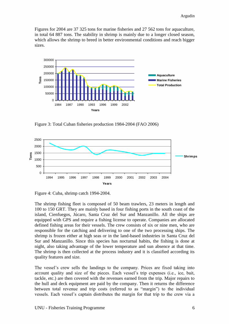
Shrimp fisheries are one of the most important in Cuban fisheries. It is carried out all

over the country. Over the years, so far the catch has decreased and so has the shrimp

catch but the lately it has been stable (Figures 3 and 4).

Argudin


0

50000

100000

150000

200000

250000

300000

1984 1987 1990 1993 1996 1999 2002

Years

To

ns

Aquaculture

Marine Fisheries

Total Production

Figures for 2004 are 37 325 tons for marine fisheries and 27 562 tons for aquaculture,

in total 64 887 tons. The stability in shrimp is mainly due to a longer closed season,

which allows the shrimp to breed in better environmental conditions and reach bigger

sizes.

Figure 3: Total Cuban fisheries production 1984-2004 (FAO 2006)

Figure 4: Cuba, shrimp catch 1994-2004.

The shrimp fishing fleet is composed of 50 beam trawlers, 23 meters in length and

100 to 150 GRT. They are mainly based in four fishing ports in the south coast of the

island, Cienfuegos, Júcaro, Santa Cruz del Sur and Manzanillo. All the ships are

equipped with GPS and require a fishing license to operate. Companies are allocated

defined fishing areas for their vessels. The crew consists of six or nine men, who are

responsible for the catching and delivering to one of the two processing ships. The

shrimp is frozen either at high seas or in the land-based industries in Santa Cruz del

Sur and Manzanillo. Since this species has nocturnal habits, the fishing is done at

night, also taking advantage of the lower temperature and sun absence at that time.

The shrimp is then collected at the process industry and it is classified according its

quality features and size.

The vessel’s crew sells the landings to the company. Prices are fixed taking into

account quality and size of the pieces. Each vessel’s trip expenses (i.e., ice, bait,

tackle, etc.) are then covered with the revenues earned from the trip. Major repairs to

the hull and deck equipment are paid by the company. Then it returns the difference

between total revenue and trip costs (referred to as “margin”) to the individual

vessels. Each vessel’s captain distributes the margin for that trip to the crew via a

0

500

1000

1500

2000

2500

1994 1995 1996 1997 1998 1999 2000 2001 2002 2003 2004

Years

To

ns

Shrimps

Argudin


predetermined share system. The captain uses his discretion to determine the share

each crew member receives. Thus, the crew has an incentive to minimise costs so that

the net income to be divided up among the crew is maximised. Because the margin is

the main source of income to the crew, a strong motivation exists to operate the

vessels as efficiently as possible. In addition, the price received by the vessel can be a

function of quality. Therefore, a high premium is placed on handling the catch in such

a way that quality is preserved (Adams et al. 2000).

The main destination market for shrimp is Spain and its demand is not fully met. The

shrimp, which is not good for export, because of melanosis or is damaged, is sold for

domestic consumption but mainly to the tourism sector in hotels and other facilities.

The price (based on the Spanish market) ranges from 10 to 18 EUR per kilo and it has

been quite stable in the last years. Maybe in the near future, the production values

could not experience a great increase, since the Cuban government is very concerned

to avoid over fishing the stocks. Therefore, the main challenge is to make the catches

more profitable by carrying out more efficient and effective fisheries, in order to take

advantage of the strong and demanding market for this product.

1.3 Objective and goals

Since the technology used now is very old, it is not possible to maximise the

effectiveness and efficiency of the catch with present vessels. New trawlers are

available in the international market and therefore the main objective of this project is

to carry out an overall analysis to find out the economic benefits from the purchase of

new vessels in fisheries companies in Cuba. Very often investment projects and new

processing introductions in Cuba are carried out without taking into consideration

important questions about the implicit risk associated with the business. The decision

makers generally do not have the tools and information needed to appreciate and

evaluate the uncertainty of the factors involved. Important decisions taken without

analysing the possibilities of success or failure can sometimes lead to serious mistakes

and great losses in both financial and production terms (Massino 2004)

Some questions were raised, during the research work, for instance: Are there any

other kind of ships, which can be used for shrimp catching under Cuban conditions

that would produce more benefits? According to the Cuban experience, beam trawlers

are the most appropriate vessels to carry out those fisheries. Stern trawlers for

example are not suitable because that activity is carried out at seas from 10 to 15

meters deep for small amounts of shrimp. Usually stern trawlers are devised for

deeper waters and larger catches. It is also believed that beam trawlers are more

manoeuvrable and therefore, it is easier for the crew to collect the shrimp from the

fishing gears. The study should take into account the increase of the catch and the

increased expenses in addition to the environmental and social issues. It is also

necessary to mention the high cost of maintenance of the current boats, due to the old

technology and the lack of spare parts. Thus, sooner than later the replacement of

these vessels will become an urgent issue.

Argudin


The main objective can be broken down into a number of goals to achieve the final

results.

Goals:

Analysis of profitability in order to determine if the new trawler would

be more profitable than the old one, considering possible risk elements.

Comparison of environmental topics, such as safety for oil spilling,

caring of the sea bottom etc.

Comparison of social topics, such as salary, crew, number of jobs and

living on board etc.

Comparison of effectiveness, taking into account mainly the proportion

of catch and by catch.

Development of a project general enough to be used in Cuban fishing

companies, under different circumstances.

Argudin


2 THEORETICAL AND PRACTICAL BACKGROUND

Profitability is, in general, the efficiency of a company or industry at generating

earnings. Some concepts related to this topic will be reviewed in this chapter but not

much can be found in the literature about profitability of fishing vessels specifically.

Many authors agree that it is necessaryto invest to make a business profitable no

matter what kind of business. It also seems reasonable that current profitability is

related to future investment and that current investment is related to future

profitability (Sloan 1996, Fairfield et al. 2002 and 2003, Richardson et al. 2004 and

2005).

Previous work also shows that dividend-paying firms tend to be more profitable

although they grow more slowly (Fama and French 2001). In Cuba, due to the

socialist system of government, most of the dividends are collected by the state in

order to support some other areas, which are not as profitable or even those, which do

not yield almost any revenues at all, like educational or health organisations.

Literature shows that accruals result in transitory variation in earnings (Sloan 1996).

This statement is consistent with other investigations (Collins and Hribar 2000, Chan

et al. 2006) that accruals predict returns on the investment.

Fairfield et al. 1996 have examined the role of particular financial statement

components and ratios in forecasting the profitability of a certain investment or

business in general. This ratio analysis was also used in determining the advisability

of investing in the project.

Getting into the particular case of calculating profitability of fishing vessels, two

computation models, Kalkyle and Minikalkyle, were put forward by Digernes (1981).

The study was carried out to develop a tool to assist fisheries stakeholders in

considering alternative investment opportunities for fishing vessels. According to

vessel owners and financing institutions if the project works in the first years, then the

inflation rate helps to manage responsibilities later on. That is the reason why only

results from one-year operations are analysed.

Both models are complementary and operate under similar bases. The difference lies

mainly in the way they present the results.

Kalkyle provides the user with a complete detailed result of the operation. The

report can be presented to a third party and also runs a sensitivity analysis,

shown both in table and diagram form.

Minikalkyle is a less complicated model. It is mainly used in the development

stage of the design of a vessel project. The users can experiment with some

input changes and several alternatives come up. The accuracy of the

information at this point is limited but it is enough to get a general idea of the

expected results.

The similarities between models are:

The operation of the vessels is the factor that produces the revenues. It takes

into account effective fishing time, amount of fishing gear used per fishing

day, catch per unit gear used and fish price.

Argudin


The cost components are related to the factor that produces it, for instance,

fuel cost is expressed as a function of the engine power and operating time.

The main results produced by the models are:

Owners’ net profit, before tax

Crew income, annual and per working day

Cash flow balance before tax

Break-even revenue and catch rates with corresponding crew income

Parameter sensitivity analysis

The model proposed in this paper is related in some ways to those outlined above. The

need for large computers for Kalkyle or programmable calculators for Minikalkyle,

which was a disadvantage at that time they were first proposed, seems to have been

overcome now with relatively easy access to computers. Microsoft Excel is a

powerful tool which is able to perform the calculations and present the results, both in

table and graph form. Another difference is that in the present study, the time value of

money was taken into account and the planning horizon is 10 years, instead of the

only one. In Digernes’ document, the ship is used in various seasons to fish different

kinds of species and using diverse fishing gears. The results for every season are

stated as well as a final summary. For Cuban shrimp trawlers it is not possible to

utilise the vessels for a different activity since trawling for fish is banned and the

revenues of using the vessels for other tasks do not cover the costs incurred. In

general terms, the model presented in this project can be seen as achieving similar

objectives to Digernes’ but taking advantage of the development of computer

technology, adapted to Cuban conditions and using some additional techniques and

methods as well.

Argudin


The Excel Model for Profitability Analysis

Model Components

Investment Revenue and Costs

Depreciation Interest

Repayment Interest Taxes Net Profit/Loss Stock Dividend

Work.Cap.Changes

Cash Movements

Cash Flow Financial Ratios

NPV IRR

Assumptions

Summary

Investment Revenue Operating Costs

Results and

Sensitivity

Scenario Summary Sensitivity Chart

Investment and

Financing

Investment Depreciation Financing

Operating

Statement

Revenue and Costs Taxation Appropriation of profit

Cash Flow

Operating Surplus Paid Taxes Repaym. & Interest Paid Dividend

Balance Sheet

Assets (Current, Fixed) Debt (Short, Long) Equity (Shares, Other)

Profitability

Measures

Project, Equity:

Net Present Value Internal Rate of Return

Graphs and Charts

Profitability (NPV, IRR)

Financial Ratios Cost Breakdown

3 METHODS

The main analytical tool in this project is a profitability assessment model designed

for Microsoft Excel. Since other aspects than economical were studied, in addition to

that model, the Analytical Hierarchy Process method was applied to support the

results. This is a well-known technique for solving multi criteria decision-making

problems.

3.1 Profitability assessment model

The model is based on one workbook with several sheets, one for each component

(Figure 5).

Figure 5: Profitability assessment model, with its main components.

Argudin


Assumptions and results

This component of the model is for the input of the assumptions for the calculations to

follow. In addition, the main results of the profitability analysis are shown here. If

needed, additional assumption sheets can be inserted before this sheet for details such

as a breakdown of the investment costs and of operational costs.

Investments and financing

This sheet includes the assumed breakdown of the investment cost related to the

project, i.e. ship costs, equipment and other investment (engineering and diverse start-

up costs).

Operating statement

This component has the purpose of calculating the revenue and costs year by year, the

income tax and other taxes, and the appropriation of profit.

Balance sheet

The balance sheet gives a more complete picture to be able to follow the forecasted

development. Also, financial ratios can be calculated. Finally, the balance sheet is

used in the model as a verification tool as many logical errors may result in a

difference between total assets on one hand and total debt and capital on the other

hand.

Cash flow

The cash flow calculation begins with the operating surplus from the operating

statement. Debtor and creditor changes are calculated on the basis of the debtors and

creditors on the balance sheet, giving cash flow before taxes.

Profitability calculations

This component of the model calculates the profitability of the investment. Two

measures are used in the model: The net present value (NPV) with a discounting

factor and the internal rate of return (IRR).

Sensitivity analysis

Sensitivity analysis for exploring and better understanding the effects of uncertainties

can be done in many different ways. Impact analysis deals with only one uncertain

item at the time, for example sales price, sales quantity or cost of ship. Scenario

analysis deals with simultaneous changes in more than one uncertain item. Excel

scenario manager is used for this purpose. The changing cells are selected and their

values for each scenario. Finally, the Monte Carlo method is used to assess the impact

of the most critical risk element, simulating normally distributed random numbers and

studying the effect on the internal rate of return.

Argudin


3.2 Analytic Hierarchy Process

The Analytic Hierarchy Process provides a proven, effective means to deal with

complex decision making and can assist in identifying and weighting selection

criteria, analysing the data collected for the criteria and expediting the decision-

making process. It helps to capture both subjective and objective evaluation measures,

providing a useful mechanism for checking the consistency of the evaluation

measures and alternatives suggested by the team thus reducing bias in decision

making. The method is especially suitable for complex decisions which involve a

comparison of decision elements, which are difficult to quantify. It is based on the

assumption that when faced with a complex decision the natural human reaction is to

cluster the decision elements according to their common characteristics.

In the Analytic Hierarchy Process, pairwise comparisons are performed by the

decision-maker and then the pairwise comparison matrix and the eigenvector are

derived to specify the weights of each parameter in the problem. The weights guide

the decision-maker in choosing the superior alternative (Ghazinoory 2006). This

method was first used by Saaty who not only introduced it (Saaty 1980), but also

utilised it in planning and anticipating for the first time (Saaty 1990). He employed

forward and backward processes to determine logical future outcomes and then found

promising control policies to attain the desired future. In the other words, Saaty’s

approach attempted to reduce the gap between logical future and desired future by

choosing the appropriate strategies.

The process facilitates the rational evaluation of these pros and cons. It supports the

pursuit of an optimal solution in a transparent manner, via:

Qualitative and quantitative decision analysis

Simple evaluation and representation of solutions through the Hierarchical

Model

Logic arguments and clearing emotions

Checking the quality of the decision

Little need of time

High acceptance

The Analytic Hierarchy Process has been applied by decision makers in countless

areas, including accounting, finance, marketing, energy resource planning,

microcomputer selection, sociology, architecture and political science (Winston

1994). Ramanathan and Ganesh (1995) employ Analytic Hierarchy for a resource

allocation problem. In that paper, the weight of each decision variable gained by

Analytic Hierarchy is used as a coefficient of that variable in the objective function. In

the present project, it was used to assess the effectiveness, environmental and social

issues involved.

Argudin


4 MODEL AND DATA ANALYSIS

4.1 Data and assumptions

The profitability odel is built up using Microsoft Excel in a way that all the data can

be inserted and changed adapting it to the characteristics of the company or business

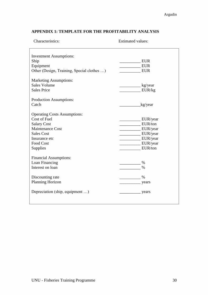
analysed. The template for the data and assumptions is shown in Appendix 1. First, in

the model, there is a work sheet, named Startup, where the main data and assumptions

are stated. All the entries are linked automatically to the sheets in which they are

going to be used, so different results can be experienced by changing the values of the

entry cells.

As mentioned previously due to the lack of some real data and the convenience of

having some inputs that could be changed by the user, a number of assumptions had

to be made. In this case, the assumptions are in italics (Figure 6). The information will

be presented in table form, so the user can more easily understand all the costs

involved in the profitability analysis. For further information, the Excel sheet, named

Assumptions and Results is Appendix 2.

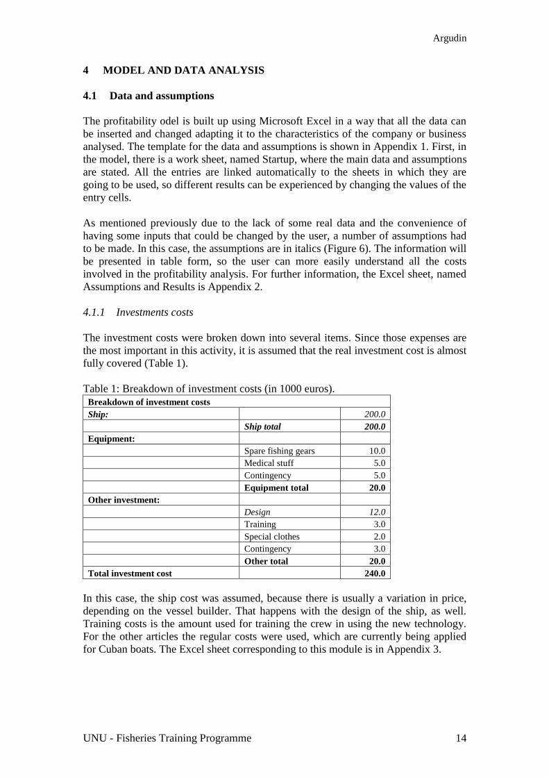
4.1.1 Investments costs

The investment costs were broken down into several items. Since those expenses are

the most important in this activity, it is assumed that the real investment cost is almost

fully covered (Table 1).

Table 1: Breakdown of investment costs (in 1000 euros).

Breakdown of investment costs

Ship: 200.0

Ship total 200.0

Equipment:

Spare fishing gears 10.0

Medical stuff 5.0

Contingency 5.0

Equipment total 20.0

Other investment:

Design 12.0

Training 3.0

Special clothes 2.0

Contingency 3.0

Other total 20.0

Total investment cost 240.0

In this case, the ship cost was assumed, because there is usually a variation in price,

depending on the vessel builder. That happens with the design of the ship, as well.

Training costs is the amount used for training the crew in using the new technology.

For the other articles the regular costs were used, which are currently being applied

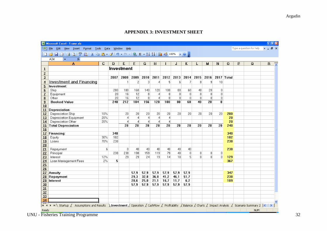
for Cuban boats. The Excel sheet corresponding to this module is in Appendix 3.

Argudin


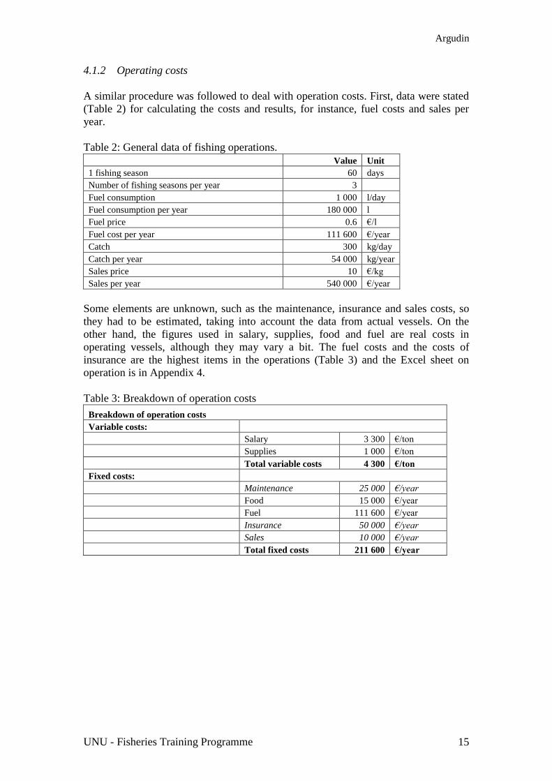
4.1.2 Operating costs

A similar procedure was followed to deal with operation costs. First, data were stated

(Table 2) for calculating the costs and results, for instance, fuel costs and sales per

year.

Table 2: General data of fishing operations.

Value Unit

1 fishing season 60 days

Number of fishing seasons per year 3

Fuel consumption 1 000 l/day

Fuel consumption per year 180 000 l

Fuel price 0.6 €/l

Fuel cost per year 111 600 €/year

Catch 300 kg/day

Catch per year 54 000 kg/year

Sales price 10 €/kg

Sales per year 540 000 €/year

Some elements are unknown, such as the maintenance, insurance and sales costs, so

they had to be estimated, taking into account the data from actual vessels. On the

other hand, the figures used in salary, supplies, food and fuel are real costs in

operating vessels, although they may vary a bit. The fuel costs and the costs of

insurance are the highest items in the operations (Table 3) and the Excel sheet on

operation is in Appendix 4.

Table 3: Breakdown of operation costs

Breakdown of operation costs

Variable costs:

Salary 3 300 €/ton

Supplies 1 000 €/ton

Total variable costs 4 300 €/ton

Fixed costs:

Maintenance 25 000 €/year

Food 15 000 €/year Fuel 111 600 €/year Insurance 50 000 €/year Sales 10 000 €/year Total fixed costs 211 600 €/year

Argudin


Fixed Cost including annuity

1000 eur/year

600

400

200

10 20 30 40 50

tons/year

Variable + Fixed Cost

Revenue

KEUR/yea

r

600

400

200

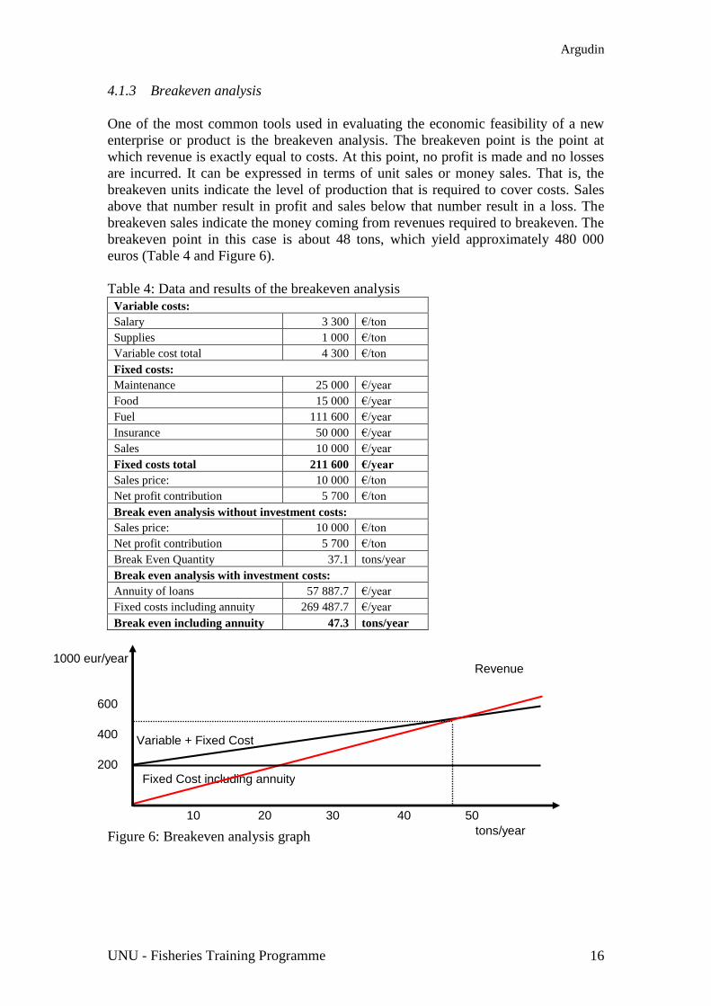
4.1.3 Breakeven analysis

One of the most common tools used in evaluating the economic feasibility of a new

enterprise or product is the breakeven analysis. The breakeven point is the point at

which revenue is exactly equal to costs. At this point, no profit is made and no losses

are incurred. It can be expressed in terms of unit sales or money sales. That is, the

breakeven units indicate the level of production that is required to cover costs. Sales

above that number result in profit and sales below that number result in a loss. The

breakeven sales indicate the money coming from revenues required to breakeven. The

breakeven point in this case is about 48 tons, which yield approximately 480 000

euros (Table 4 and Figure 6).

Table 4: Data and results of the breakeven analysis

Variable costs:

Salary 3 300 €/ton

Supplies 1 000 €/ton

Variable cost total 4 300 €/ton

Fixed costs:

Maintenance 25 000 €/year

Food 15 000 €/year

Fuel 111 600 €/year

Insurance 50 000 €/year

Sales 10 000 €/year

Fixed costs total 211 600 €/year

Sales price: 10 000 €/ton

Net profit contribution 5 700 €/ton

Break even analysis without investment costs:

Sales price: 10 000 €/ton

Net profit contribution 5 700 €/ton

Break Even Quantity 37.1 tons/year

Break even analysis with investment costs:

Annuity of loans 57 887.7 €/year

Fixed costs including annuity 269 487.7 €/year

Break even including annuity 47.3 tons/year

Figure 6: Breakeven analysis graph

Argudin


-150

-100

-50

0

50

2007 2008 2009 2010 2011 2012 2013 2014 2015 2016 2017

Years

10

00

Eu

r

-400

-300

-200

-100

0

100

200

2007

2008

2009

2010

2011

2012

2013

2014

2015

2016

2017

Years

1000 E

ur

Total Cash Flow & Capital

Net Cash Flow & Equity

4.2 Cash flow analysis

In this analysis, two main elements were studied. Total cash flow and capital, which

shows a positive value throughout all the years, except for the first one, when the

starting financing is deducted. The net cash flow and equity, is below zero in the first

two years, mainly because debtors are very high, but after that period, there is an

increasing trend. Both flows are presented in Figure 7 (Appendixes 5 to 7).

Figure 7: Cash flow behaviour

4.3 Profitability analysis

In this analysis the internal rate of return and the net present value were evaluated as

well as the most important financial ratios, some other ratios are presented in

Appendix 6.

The Internal rate of return is a capital budgeting method used by firms to decide

whether they should make long-term investments. It is the return rate, which can be

earned on the invested capital, i.e. the yield on the investment. A project is a good

investment proposition if its internal rate of return is greater than the rate of interest

that could be earned by alternative investments (investing in other projects, buying

bonds, even putting the money in a bank account). Mathematically it is defined as any

discount rate that results in a net present value of zero of a series of cash flows. In this

project, the internal rate of return of equity is 21%, after 10 years (Figure 8).

Figure 8: Internal rate of return

http://en.wikipedia.org/wiki/Capital_budgeting

http://en.wikipedia.org/wiki/Investment

http://en.wikipedia.org/wiki/Discount_rate

http://en.wikipedia.org/wiki/Net_present_value

Argudin


0%

5%

10%

15%

20%

25%

2007 2008 2009 2010 2011 2012 2013 2014 2015 2016 2017

Years

%

0

5

10

15

20

2007

2008

2009

2010

2011

2012

2013

2014

2015

2016

2017

Years

The net present value of a project or investment is defined as the sum of the present

values of the annual cash flows minus the initial investment. The annual cash flows

are the net benefits (revenues minus costs) generated from the investment during its

lifetime. These cash flows are discounted or adjusted by incorporating the uncertainty

and time value of money. It is one of the most robust financial evaluation tools to

estimate the value of an investment. If a project has a positive net present value, then

it is generating more cash than is needed to service its debt and provide the required

return to shareholders (Brigham and Houston 2004). So the study investment, with net

present value equals 39 000 euros acceptable, but the discounted payback period is

too long, eight years (Figure 9).

Figure 9: Net present value

The Net current ratio is a comparison of a firm’s current assets to its current liabilities.

It is an indication of a firm’s market liquidity and ability to meet short-term debt

obligations. If current liabilities exceed current assets (the current ratio is below one),

then the company may have problems meeting its short-term obligations. It does not

happen in this situation, since the company has an increasing ratio every year (Figure

10).

Figure 10: Net current ratio

http://en.wikipedia.org/wiki/Asset

http://en.wikipedia.org/wiki/Liabilities

http://en.wikipedia.org/wiki/Market_liquidity

Argudin


0

10

20

2007

2008

2009

2010

2011

2012

2013

2014

2015

2016

2017

Years

0123

2007

2008

2009

2010

2011

2012

2013

2014

2015

2016

2017

Years

Liquid current ratio (quick current ratio): The acid-test or quick ratio measures the

ability of a company to use its “near cash” or quick assets to immediately extinguish

its current liabilities. Quick assets include those current assets that presumably can be

quickly converted into cash at close to their book values. Such items are cash, stock

investments, and accounts receivable. This ratio implies a liquidation approach and

does not recognise the revolving nature of current assets and liabilities. The behaviour

of this ratio is very similar to the previous (Figure 11) (Appendix 7).

Figure 11: Liquid current ratio

Debt Service Coverage is a measure of a company’s or an individual’s ability to

cover, or pay off debt. It refers to the amount of cash or cash flow required to pay off

a debt, and how much the total debt actually is. The higher this ratio is, the easier it is

to borrow money for the investment. In the project, some problems are faced in the

first four years, but after that period, the ratio is over 1.5, which is a good one, in

general terms (Figure 12).

Figure 12: Debt service coverage

Argudin


4.4 Sensitivity analysis

A sensitivity analysis is a good method to understand uncertainty in any type of

financial model. Its objective is to identify critical inputs of the financial model and

how they impact the results. This is particularly important in investments where a

change of say 10% in an input can make the project unprofitable. It is, therefore,

essential to understand the dynamics of the underlying variables. This analysis was

performed using two methods, impact analysis and scenario analysis.

4.4.1 Impact analysis

The main goal of the study is to evaluate the changes in the internal rate of return of

the equity, when variations of the inputs are introduced. The process was carried out

by changing one element at the time, sales price, sales quantity or ship cost. Then the

output shows that sales price is the most critical component in this case, a decrease of

only 10% would lead to an internal rate of return equal to zero. This also happens

when the sales quantity is diminished by 10%, the internal rate of return would drop

by 17%, from 21% to 4%. On the other hand, a variation of the ship cost does not

affect this economic indicator too much. The results are displayed in Table 5 and

Figure 13.

Table 5: Impact analysis on internal rate of return of equity showing IRR of equity

against deviation for sales price, quantity and ship cost.

Variation Sales price

variation IRR=21%

Sales quantity

variation IRR=21%

Ship cost

variation IRR=21%

-50% 50% 0% 50% 0% 50% 37%

-40% 60% 0% 60% 0% 60% 33%

-30% 70% 0% 70% 0% 70% 30%

-20% 80% 0% 80% 0% 80% 26%

-10% 90% 0% 90% 4% 90% 24%

0% 100% 21% 100% 21% 100% 21%

10% 110% 52% 110% 38% 110% 18%

20% 120% 86% 120% 55% 120% 16%

30% 130% 122% 130% 74% 130% 14%

40% 140% 160% 140% 92% 140% 12%

50% 150% 198% 150% 112% 150% 11%

Argudin


0%

10%

20%

30%

40%

50%

60%

70%

80%

90%

100%

-50% -40% -30% -20% -10% 0% 10% 20% 30% 40% 50%

Deviation

IRR

of

Eq

uit

ySales Price

Sales Quantity

Ship cost

Figure 13: Impact analysis on internal rate of return of equity showing IRR of equity

against deviation for sales price, quantity and ship cost.

4.4.2 Scenario analysis

A scenario analysis is a special case of sensitivity analysis where a pre-determined set

of possible outcomes is identified. It is highly effective as a communication tool to

describe the uncertainty of a project. It bounds the outcomes of a project and

communicates the risks associated with the project. It differs from the previous

method because in this case, the three elements are changed at the same time. First

two scenarios were defined, pessimistic and optimistic, using Microsoft Excel

scenario manager. In the pessimistic scenario it was assumed that the ship cost, the

sales quantity and the sales price were 10% worse than the current values and in the

optimistic, the assumptions were the other way around. Results are shown in Table 6.

Table 6: Scenario analysis summary

Scenario summary Current values: Pessimistic Optimistic

Changing cells:

Ship_cost 100% 110% 90%

Sales_quantity 100% 90% 110%

Sales_price 100% 90% 110%

Result cells:

NPV_total_capital 25 -297 370

NPV_equity 39 -282 383

IRR_total_capital 17% 0% 42%

IRR_equity 21% 0% 79%

Argudin


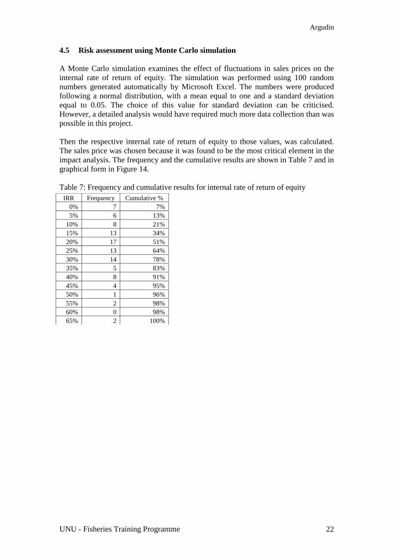
4.5 Risk assessment using Monte Carlo simulation

A Monte Carlo simulation examines the effect of fluctuations in sales prices on the

internal rate of return of equity. The simulation was performed using 100 random

numbers generated automatically by Microsoft Excel. The numbers were produced

following a normal distribution, with a mean equal to one and a standard deviation

equal to 0.05. The choice of this value for standard deviation can be criticised.

However, a detailed analysis would have required much more data collection than was

possible in this project.

Then the respective internal rate of return of equity to those values, was calculated.

The sales price was chosen because it was found to be the most critical element in the

impact analysis. The frequency and the cumulative results are shown in Table 7 and in

graphical form in Figure 14.

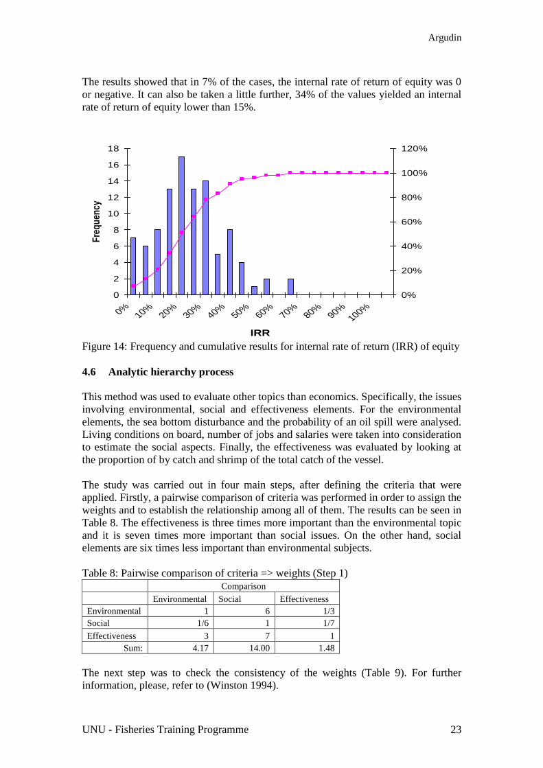
Table 7: Frequency and cumulative results for internal rate of return of equity

IRR Frequency Cumulative %

0% 7 7%

5% 6 13%

10% 8 21%

15% 13 34%

20% 17 51%

25% 13 64%

30% 14 78%

35% 5 83%

40% 8 91%

45% 4 95%

50% 1 96%

55% 2 98%

60% 0 98%

65% 2 100%

Argudin


0

2

4

6

8

10

12

14

16

18

0%10%

20%30%

40%50%

60%70%

80%90%

100%

IRR

Fre

qu

ency

0%

20%

40%

60%

80%

100%

120%

The results showed that in 7% of the cases, the internal rate of return of equity was 0

or negative. It can also be taken a little further, 34% of the values yielded an internal

rate of return of equity lower than 15%.

Figure 14: Frequency and cumulative results for internal rate of return (IRR) of equity

4.6 Analytic hierarchy process

This method was used to evaluate other topics than economics. Specifically, the issues

involving environmental, social and effectiveness elements. For the environmental

elements, the sea bottom disturbance and the probability of an oil spill were analysed.

Living conditions on board, number of jobs and salaries were taken into consideration

to estimate the social aspects. Finally, the effectiveness was evaluated by looking at

the proportion of by catch and shrimp of the total catch of the vessel.

The study was carried out in four main steps, after defining the criteria that were

applied. Firstly, a pairwise comparison of criteria was performed in order to assign the

weights and to establish the relationship among all of them. The results can be seen in

Table 8. The effectiveness is three times more important than the environmental topic

and it is seven times more important than social issues. On the other hand, social

elements are six times less important than environmental subjects.

Table 8: Pairwise comparison of criteria => weights (Step 1)

Comparison

Environmental Social Effectiveness

Environmental 1 6 1/3

Social 1/6 1 1/7

Effectiveness 3 7 1

Sum: 4.17 14.00 1.48

The next step was to check the consistency of the weights (Table 9). For further

information, please, refer to (Winston 1994).

Argudin


Table 9: Checking consistency (Step 2)

Normalised:

Environmental Social Effectiveness Weights A*w' A*w'/w'

Environmental 0.24 0.43 0.23 0.30 0.93 3.10

Social 0.04 0.07 0.10 0.07 0.21 3.02

Effectiveness 0.72 0.50 0.68 0.63 2.01 3.18

1.00 1.00 1.00 1.00 M= 3.10

CI = 0.051

CI/RI= 0.087

Consistency

Once it has been stated the weights are consistent then the third step is to compare the

two vessels, the old and the new, according to the different criteria, that is

environmental, social and effectiveness elements. The weights are given in the range

of 1 to 10, meaning the times that a characteristic is stronger compared to the other

boat (Tables 10 to 12).

Table 10: Pairwise comparison of alternatives => weights (environmental) (Step 3)

Environmental Comparison

Old New

Old 1 1/3

New 3 1

Sum: 4.00 1.33

Table 11: Pairwise comparison of

alternatives => weights (social) (Step 3)

Social Comparison

Old New

Old 1 1/9

New 9 1

Sum: 10.00 1.11

Table 12: Pairwise comparison of

alternatives => weights

(effectiveness) (Step 3)

Effectiveness Comparison

Old New

Old 1 1/5

New 5 1

Sum: 6.00 1.20

In sum, the new trawler is three times better than the old one in the environmental

issue, nine times better in the social aspects and five times better regarding the

effectiveness.

The fourth step is to calculate weighted final scores, combining the criteria with the

alternatives, as summarised in Table 13. Therefore, the final scores are determined by

multiplying the weights of the criteria, environmental, social and effectiveness with

Environmental Normalised

Old New

Old 0.25 0.25

New 0.75 0.75

Sum: 1.00 1.00

Social Normalised

Old New

Old 0.10 0.10

New 0.90 0.90

Sum: 1.00 1.00

Effectiveness Normalised

Old New

Old 0.17 0.17

New 0.83 0.83

Sum: 1.00 1.00

Argudin


0,00

0,20

0,40

0,60

0,80

1,00

Enviromental

SocialEfectiveness

Old

New

0,000

0,200

0,400

0,600

Enviromental

SocialEfectiveness

Old

New

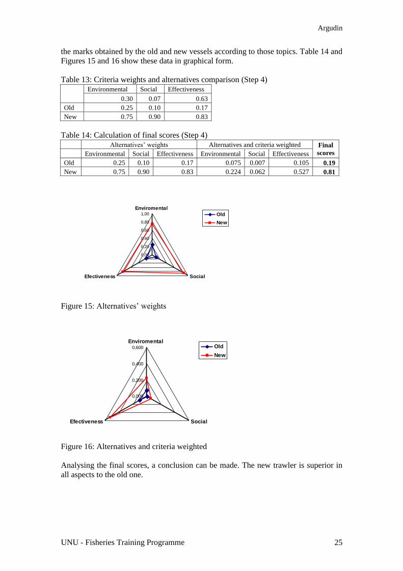
the marks obtained by the old and new vessels according to those topics. Table 14 and

Figures 15 and 16 show these data in graphical form.

Table 13: Criteria weights and alternatives comparison (Step 4)

Environmental Social Effectiveness

0.30 0.07 0.63

Old 0.25 0.10 0.17

New 0.75 0.90 0.83

Table 14: Calculation of final scores (Step 4)

Alternatives’ weights Alternatives and criteria weighted Final

scores Environmental Social Effectiveness Environmental Social Effectiveness

Old 0.25 0.10 0.17 0.075 0.007 0.105 0.19

New 0.75 0.90 0.83 0.224 0.062 0.527 0.81

Figure 15: Alternatives’ weights

Figure 16: Alternatives and criteria weighted

Analysing the final scores, a conclusion can be made. The new trawler is superior in

all aspects to the old one.

Argudin


5 CONCLUSIONS AND RECOMMENDATIONS

In order to achieve the most important objective of the research, it is vital to state if

the project should be carried out or not. Therefore, the purpose of this chapter is to

answer that question, summarising the methods and techniques applied and the results

obtained. The breakeven analysis was applied to find out the necessary quantity of

shrimp to be caught each year in order to have an annual profit greater than zero. The

result is that a minimum of 48 tons is needed to keep the business running properly. In

other words, with current prices, the catch has to be over that value to assure at least

480 000 euros, in order to get some profit. Taking into account that expected annual

catch is 54 tons, the margin is not so big. Therefore, a small decrease in the fisheries

or in the sales price, would lead the company to run losses.

The general cash flow of the project is rather stable, throughout the planning horizon.

However, in the first year of operation, the organisation would experience some cash

flow problems. The net cash flow after that period increases every year. It is even

higher in the last years forecasted, when debt is already paid off. Therefore, the

company would be financially healthy in the short term and has no problem with

liquidity. In the profitability analysis, the internal rate of return = 21%, meaning the

investment is feasible. The net present value = 39 000 euros is acceptable, however,

the discounted payback period is very long. The ratios studied, net current, liquid

current and debt service coverage have a positive and increasing behaviour as well.

In the impact analysis, the sales price came out to be the most critical element, since a

decrease of only 10% would make the internal rate of return 0. This variable was

taken to perform the scenario analysis, as well as the ship costs and the sales quantity.

The pessimistic scenario yielded very bad results, with a negative net present value

and internal rate of return = 0% while the optimistic scenario had opposite results.

Consequently, the project is highly risky, because those elements were only modified

by 10% and the results experienced a great variation from the original values. Then a

Monte Carlo simulation was performed for the most sensitive aspect, that is sales

price. The outcome confirms the great risk of the investment, since 34 cases out of

100, produced an insufficient internal rate of return. At last, an analytic hierarchy

process was carried out to asses some other aspects. Those are effectiveness, social

and environmental topics. The comparison between the two vessels on these matters

shows that the new one is much better than the old one.

Summing up, it is strongly advisable to put into effect the purchasing project, to boost

the shrimp fisheries and therefore the Cuban economy. Nevertheless, the high risk

associated with the investment has to be assessed very closely in order to minimise it.

Finally, it is essential to remark that the research made can be a very useful tool to

evaluate the feasibility of investments and the risks associated to it. In Cuba, it would

mean a necessary change in the mind and way of work of decision makers. Having the

expected result of a project by a scientific and overall study would result in

minimising losses in both financial and production terms. The analysis proposed here

can be applied not only to fishing vessels but also to almost every investment in the

world, just by adapting the model to the circumstances of the particular task. So, it is

strongly recommended to implement it as a valuable evaluation instrument and

guideline for investment projects.

Argudin


ACKNOWLEDGEMENTS

To be able to succeed in a course like this one requires team work. It does not only

depend on the fellows’ attitude but, also on the support and commitment of the

persons related to it. It has been a wonderful experience in both my professional and

personal life to have participated in The United Nations University-Fisheries Training

Programme. I would like to express my deepest appreciation to Dr. Tumi Tomasson,

Programme Director, Mr. Thor H. Asgeirsson, Deputy Programme Director and to

Ms. Sigridur Ingvarsdottir, Programme Officer, for the opportunity of professional

growth that will enable me to become a better specialist in the near future and for their

guidance and collaboration during the process. I am very thankful to my supervisor,

Dr. Páll Jensson, for his valuable assistance and excellent recommendations, which

led me to the final results. Last but, not least, I would like to acknowledge the

encouragements and support of all my colleagues from the programme. Thank you all

so much.

Argudin


LIST OF REFERENCES

Adams, C., Sanchez Viga, P. and Garcia Alvarez, A. 2000. An overview of the Cuban

commercial fishing industry and recent changes in management structure and

objectives. Institute of Food and Agricultural Sciences, University of Florida,

Gainsville, EDIS document FE 218, 8pp. Available at edis.ifas.ufl.edu.

Alen de Llano Massino. 2004. Financial and biological model for intensive culture of

Tilapia. United Nations University-Fisheries Training Programme in Iceland (UNU-

FTP). http://www.unuftp.is/Proj04/AlenPRF04.pdf

Brigham, E.F. and Houston, J.F. 2004. Fundamentals of Financial Management.10th

ed.International Students Edition (ISE).pp.387- 421.

Chan, K., Chan, L.K.C., Jegadeesh, N., Lakonishok, J. 2006. Earnings quality and

stock returns. Journal of Business 79, 1041–1082.

Collins, D.W., Hribar, P. 2000. Earnings-based and accrual-based market anomalies:

one effect or two? Journal of Accounting and Economics 29, 101–123.

Digernes, T. 1981. "Simple Computation Models for Calculating Profitability of

Fishing Vessels". Proceedings of the NATO Symposium on Applied Operations

Research in Fishing, August 1979, Tronheim, Norway, K.B. Haley (ed). Plenum

Press, New York, 173-186.

Fairfield, P. M., Sweeney R. J., and Yohn T. L. 1996. Accounting Classification and

the Predictive Content of Earnings. The Accounting Review 71, 337–355.

Fairfield, P.M., Whisenant, S., Yohn, T.L. 2002. The differential persistence of

accruals and cash flows for future operating income versus future return on assets.

Unpublished working paper. Georgetown University, Washington, DC.

Fairfield, P.M., Whisenant, S., Yohn, T.L. 2003. Accrued earnings and growth:

implications for future profitability and market mispricing. The Accounting Review

78, 353–371.

Fama, E.F., French, K.R. 2001. Disappearing dividends: changing firm characteristics

or lower propensity to pay. Journal of Financial Economics 60, 3–43.

Ghazinoory S. 2006. Using AHP and L.P. for choosing the best alternatives ...,

Applied Mathematics and Computation, doi:10.1016/j.amc.2006.05.178.

Ramanathan R, Ganesh L.S. 1995.Using AHP for resource allocation problems, Eur.

J. Oper. Res. 80 417.

Richardson, S.A., Sloan, R.G., Soliman, M.T., Tuna, I. 2004. The implications of

accounting distortions and growth for accruals and profitability. Unpublished

working paper. University of Pennsylvania, Philadelphia, PA.

http://www.unuftp.is/Proj04/AlenPRF04.pdf

Argudin


Richardson, S.A., Sloan, R.G., Soliman, M.T., Tuna, I. 2005. Accrual reliability,

earnings persistence, and stock prices. Journal of Accounting and Economics 39, 437–

485.

Saaty, T. 1980. The Analytic Hierarchy Process. Mc Graw-Hill, New York. Revised

and extended 1988.

Saaty, T. 1990. Decision-Making for Leaders. Pittsburg University Edition.

Sloan, R.G. 1996. Do stock prices fully reflect information in accruals and cash flows

about future earnings? The Accounting Review 71, 289–315.

Winston, W.L. 1994. Operations research: Application and algorithms. 3rd

ed,

Belmont, California: Waldsworth Publishing Company.

Argudin


APPENDIX 1: TEMPLATE FOR THE PROFITABILITY ANALYSIS

Characteristics: Estimated values:

Investment Assumptions:

Ship __________ EUR

Equipment __________ EUR

Other (Design, Training, Special clothes …) __________ EUR

Marketing Assumptions:

Sales Volume __________ kg/year

Sales Price __________ EUR/kg

Production Assumptions:

Catch __________kg/year

Operating Costs Assumptions:

Cost of Fuel __________ EUR/year

Salary Cost __________ EUR/ton

Maintenance Cost __________ EUR/year

Sales Cost __________ EUR/year

Insurance etc __________ EUR/year

Food Cost __________ EUR/year

Supplies __________ EUR/ton

Financial Assumptions:

Loan Financing __________ %

Interest on loan __________ %

Discounting rate __________ %

Planning Horizon __________ years

Depreciation (ship, equipment …) __________ years

Argudin


APPENDIX 2: ASSUMPTIONS AND RESULTS SHEET

Argudin


APPENDIX 3: INVESTMENT SHEET

Argudin


APPENDIX 4: OPERATION SHEET

Argudin


APPENDIX 5: CASH FLOW SHEET

Argudin


APPENDIX 6: PROFITABILITY SHEET

6 APPENDIX 7: BALANCE SHEET

Argudin


profitability analysis of the investment in · pdf fileprofitability analysis of the...

Documents