program for north american mobility in higher education · program for north american mobility in...
TRANSCRIPT

Program for North American Program for North American Mobility in Higher EducationMobility in Higher EducationIntroducing Introducing PProcess rocess IIntegration for ntegration for EEnvironmental nvironmental
CControl in ontrol in EEngineering Curricula.ngineering Curricula.P.I.E.C.E.P.I.E.C.E.
Module: 12Module: 12““NETWORK PINCH ANALYSISNETWORK PINCH ANALYSIS””
Created at:Created at:Texas A&M UniversityTexas A&M University
College Station, TX. JanuaryCollege Station, TX. January--May 2005May 2005
Miguel Velazquez

22
MODULE 12. NETWORK PINCH ANALYSISN.A.M.P. / P.I.E.C.E.
PURPOSEPURPOSEThe intention of this Module is to provide a general view The intention of this Module is to provide a general view of the available techniques for the retrofit and operability of the available techniques for the retrofit and operability analysis of existing heat and mass exchange networks.analysis of existing heat and mass exchange networks.

33
MODULE 12. NETWORK PINCH ANALYSISN.A.M.P. / P.I.E.C.E.
PREPRE--REQUISITESREQUISITESIn order to achieve a better understanding of the contents of In order to achieve a better understanding of the contents of this Module, the student or reader are required to possess a this Module, the student or reader are required to possess a background of specific areas of chemical engineering such as background of specific areas of chemical engineering such as classic thermodynamic, mass transfer and heat transfer. These classic thermodynamic, mass transfer and heat transfer. These subjects are part of basic science of chemical engineering and subjects are part of basic science of chemical engineering and must be contained into its curricula.must be contained into its curricula.
A Process Introduction Module review prior to this Module is A Process Introduction Module review prior to this Module is recommended too. In such, an overview of Pinch Technology recommended too. In such, an overview of Pinch Technology and Heat Recovery Network can be found to help you begin and Heat Recovery Network can be found to help you begin with the Network Pinch Analysis subject.with the Network Pinch Analysis subject.

44
MODULE 12. NETWORK PINCH ANALYSISN.A.M.P. / P.I.E.C.E.
AUDIENCE TARGET.AUDIENCE TARGET.The Network Pinch Module is addressed to last year bachelor The Network Pinch Module is addressed to last year bachelor degree and degree and MScMSc students in chemical engineering. Particularly students in chemical engineering. Particularly it will be useful for practicing engineers and even teachers of it will be useful for practicing engineers and even teachers of plant design and pollution prevention courses. plant design and pollution prevention courses.

55
MODULE 12. NETWORK PINCH ANALYSISN.A.M.P. / P.I.E.C.E.
STRUCTURE:STRUCTURE:
TIER I. FUNDAMENTALSTIER I. FUNDAMENTALS
TIER II. CASE STUDIESTIER II. CASE STUDIES
TIER III. OPEN ENDED PROBLEMSTIER III. OPEN ENDED PROBLEMS

TIER ITIER I
77
MODULE 12. NETWORK PINCH ANALYSISN.A.M.P. / P.I.E.C.E.
TIER I: FUNDAMENTALSTIER I: FUNDAMENTALS
1.1. HEAT RECOVERY NETWORKS (HEN).HEAT RECOVERY NETWORKS (HEN).2.2. STEADY STATE SIMULATION of STEADY STATE SIMULATION of HENsHENs..3.3. OPERABILITY ANALYSIS of OPERABILITY ANALYSIS of HENsHENs..4.4. RETROFIT of RETROFIT of HENsHENs..5.5. MASS EXCHANGE NETWORKS (MEN).MASS EXCHANGE NETWORKS (MEN).6.6. OPERABILITY ANALYSIS of OPERABILITY ANALYSIS of MENsMENs..

1.1.-- HEAT EXCHANGE NETWORK HEAT EXCHANGE NETWORK (HEN)(HEN)
1.1 Introduction1.1 Introduction1.2 Basic Concepts.1.2 Basic Concepts.1.3 Cost Target.1.3 Cost Target.1.4 Heat Recovery Network (HEN) Design.1.4 Heat Recovery Network (HEN) Design.

99
MODULE 12. NETWORK PINCH ANALYSISN.A.M.P. / P.I.E.C.E.
One of the main advantages of Pinch Technology over
conventional design methods is the ability to set energy and capital cost
targets for an individual process or for an entire production site ahead of
design. Therefore, ahead of identifying any specific project, we know
the scope for energy savings and investment requirements.
1.1 Introduction.1.1 Introduction.

1010
MODULE 12. NETWORK PINCH ANALYSISN.A.M.P. / P.I.E.C.E.
Most industrial processes involve transfer of heat either from one process stream to another process stream (interchanging) or from an utility stream to process stream.

1111
MODULE 12. NETWORK PINCH ANALYSISN.A.M.P. / P.I.E.C.E.
What is industry challenged about energy What is industry challenged about energy consumption and recovery?consumption and recovery?

1212
MODULE 12. NETWORK PINCH ANALYSISN.A.M.P. / P.I.E.C.E.
HeatRecovery
Energyrequirements
In the present energy crisis scenario all over the world, the target of any industrial process designer is to maximizes the process-to-process heat recovery and to minimize the utility (energy) requirements.

1313
MODULE 12. NETWORK PINCH ANALYSISN.A.M.P. / P.I.E.C.E.
To meet the goal of maximize energy recovery or minimum energy requirement (MER) an appropriate heat exchanger network (HEN) isrequired.
2 5 7
1
246
H
H
H
HC C C
Steam
Coldwater
341.1
528.0
412.8
320
451.4 427.4 505.6
7 3
1
246
5
63
2
4
H
Steam
Coldwater
22.4
217.5 16.286.3
341.1
412.8
5
1
H CHeater Cooler Heat exchanger
Fig. 1.1 (a) The non-integrated solution, (b) The optimally integrated solution Reference.
a) Traditional design:Cost operating 250,838 $/yearCost capital 4,937 $/year
b) Technology Pinch approach:Cost operating 24,077.00 $/yearCost capital 4,180.00 $/year
Hot Stream Cold Stream

1414
MODULE 12. NETWORK PINCH ANALYSISN.A.M.P. / P.I.E.C.E.
General Process ImprovementsGeneral Process ImprovementsIn addition to energy conservation studies, Pinch Technology enables process
engineers to achieve the following general process improvements:
Update or Modify Process Flow Diagram: Pinch quantifies the savings available by changing the process itself. It shows where process change reduce the overall energy target, not just local energy consummation.
Conduct Process Simulation Studies: Pinch replace the old energy studies with information that can be easily updating using simulation. Such simulation studies can help avoid unnecessary capital costs by identifying energy savings with a smaller investment before the projects are implemented.
Set Practical targets: By taking in account practical constrains (difficult fluids, layout, safety, etc.), theoretical targets are modified so that they can be realistically achieved. Comparing practical with theoretical targets quantifies opportunities “lost” by constraints - a vital insight for long term development.
De-bottlenecking: Pinch analysis when specifically applied to debottleneckingstudies, can lead to the following benefits compared to a conventional revamp:
– Reduction in capital costs.
– Decrease in specific energy demand giving a more competitive production facilities.

1515
MODULE 12. NETWORK PINCH ANALYSISN.A.M.P. / P.I.E.C.E.
1.2 Basic Concepts1.2 Basic Concepts
1.1. Identification of the hot, cold and utility streams in the Identification of the hot, cold and utility streams in the process.process.
2.2. Thermal data extraction for process and utility stream.Thermal data extraction for process and utility stream.
3.3. Selection of Initial Selection of Initial ΔΔTTMINMIN value.value.
4.4. Construction of Composite Curves and Grand Construction of Composite Curves and Grand Composite Curve.Composite Curve.
1616
MODULE 12. NETWORK PINCH ANALYSISN.A.M.P. / P.I.E.C.E.
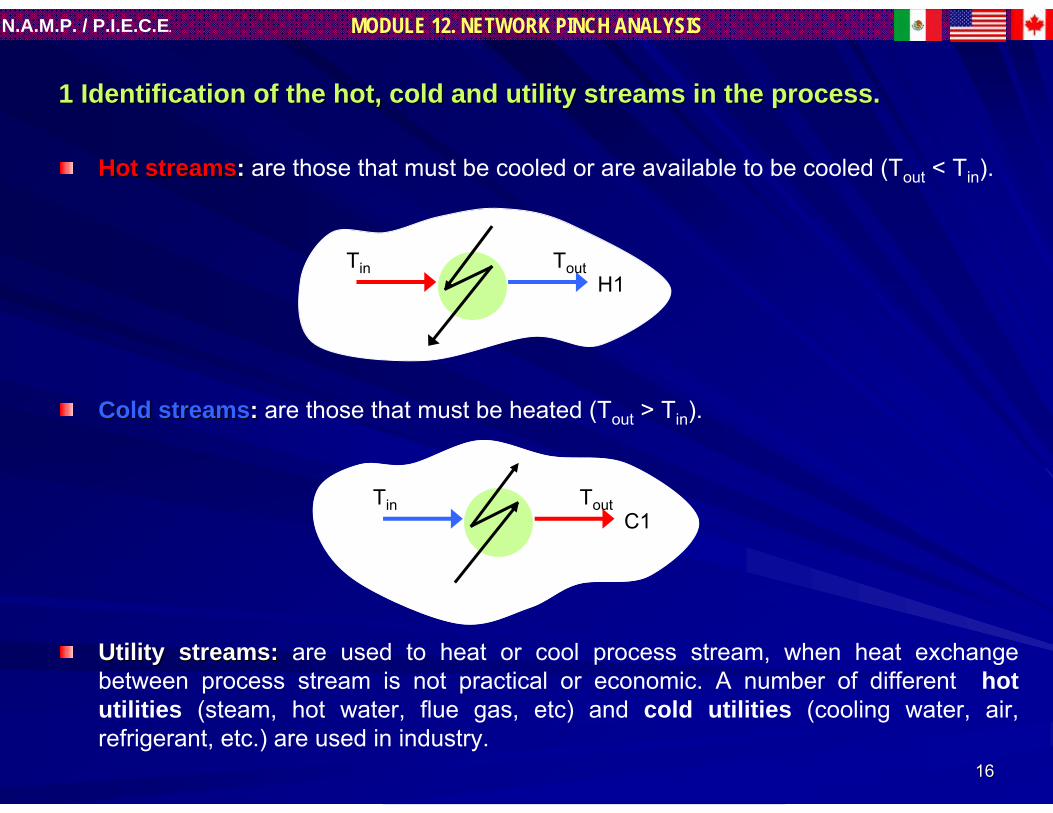
1 Identification of the hot, cold and utility streams in the pro1 Identification of the hot, cold and utility streams in the process.cess.
Hot streamsHot streams:: are those that must be cooled or are available to be cooled (Tout < Tin).
Cold streamsCold streams:: are those that must be heated (Tout > Tin).
Utility streams:Utility streams: are used to heat or cool process stream, when heat exchange between process stream is not practical or economic. A number of different hot utilities (steam, hot water, flue gas, etc) and cold utilities (cooling water, air, refrigerant, etc.) are used in industry.
Tin ToutH1
Tin ToutC1

1717
MODULE 12. NETWORK PINCH ANALYSISN.A.M.P. / P.I.E.C.E.
2 Thermal data extraction for process and utility stream.
For each hot, cold and utility stream identified, the following thermal data is extracted for the process material and heat balance flow sheet:Supply temperature TS, the temperature which the stream is available.Target temperature TT, the temperature the stream must be taken to.Heat capacity flow rate (CP), the product of flow rate and specific heat.Enthalpy change H, H = CP(TS - TT)
Stream Number
Stream name
Supply Temperature
(oC)
Target Temperature
(oC)
Heat Capacity
Flow Rate (kW/oC)
Enthalpy Change
(kW)
1 Feed 60 205 20 2900
2 Reactor out 270 160 18 1980
3 Product 220 70 35 5250
4 Recycle 160 210 50 2500
Table 1.1 Typical Stream Data
1818
MODULE 12. NETWORK PINCH ANALYSISN.A.M.P. / P.I.E.C.E.
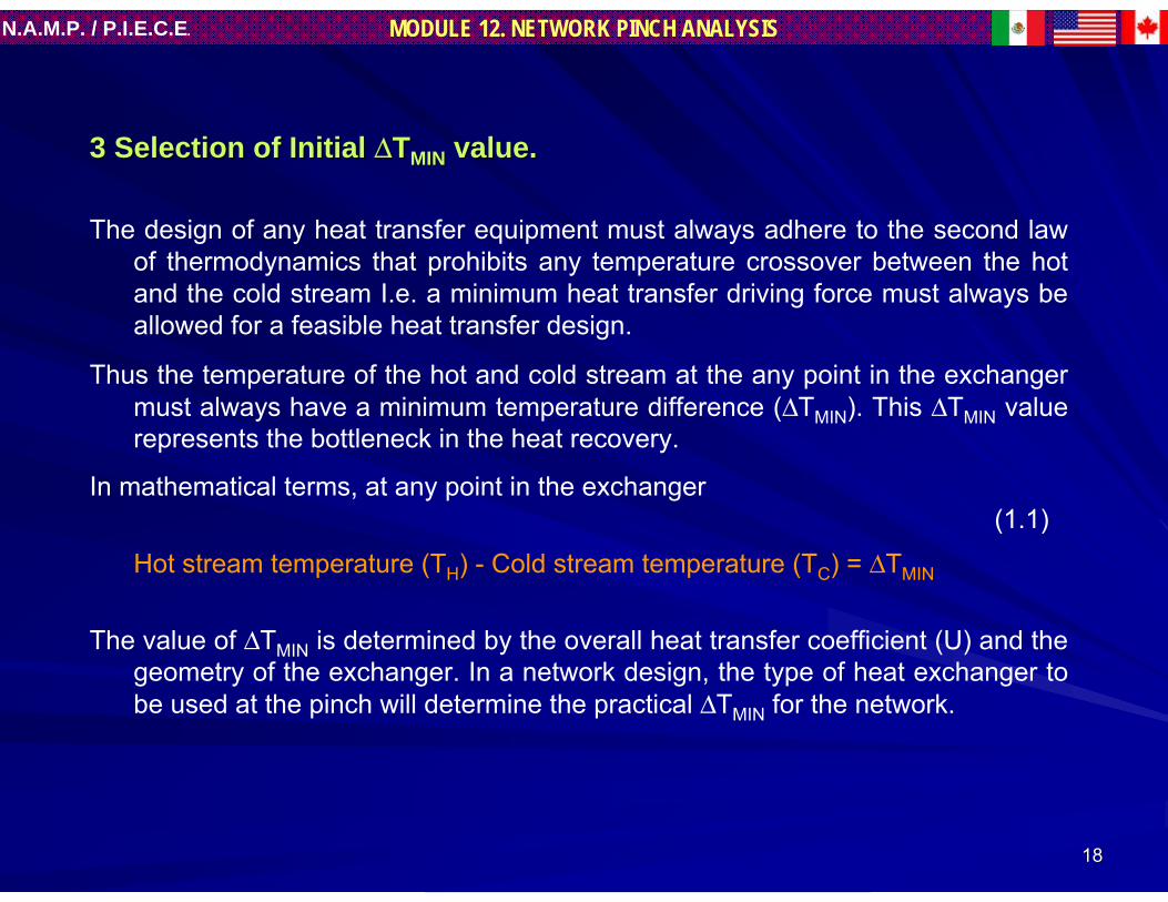
3 Selection of Initial 3 Selection of Initial ΔΔTTMINMIN value.value.
The design of any heat transfer equipment must always adhere to the second law of thermodynamics that prohibits any temperature crossover between the hot and the cold stream I.e. a minimum heat transfer driving force must always be allowed for a feasible heat transfer design.
Thus the temperature of the hot and cold stream at the any point in the exchanger must always have a minimum temperature difference (ΔTMIN). This ΔTMIN value represents the bottleneck in the heat recovery.
In mathematical terms, at any point in the exchanger
Hot stream temperature (TH) - Cold stream temperature (TC) = ΔTMIN
The value of ΔTMIN is determined by the overall heat transfer coefficient (U) and the geometry of the exchanger. In a network design, the type of heat exchanger to be used at the pinch will determine the practical ΔTMIN for the network.
(1.1)
1919
MODULE 12. NETWORK PINCH ANALYSISN.A.M.P. / P.I.E.C.E.
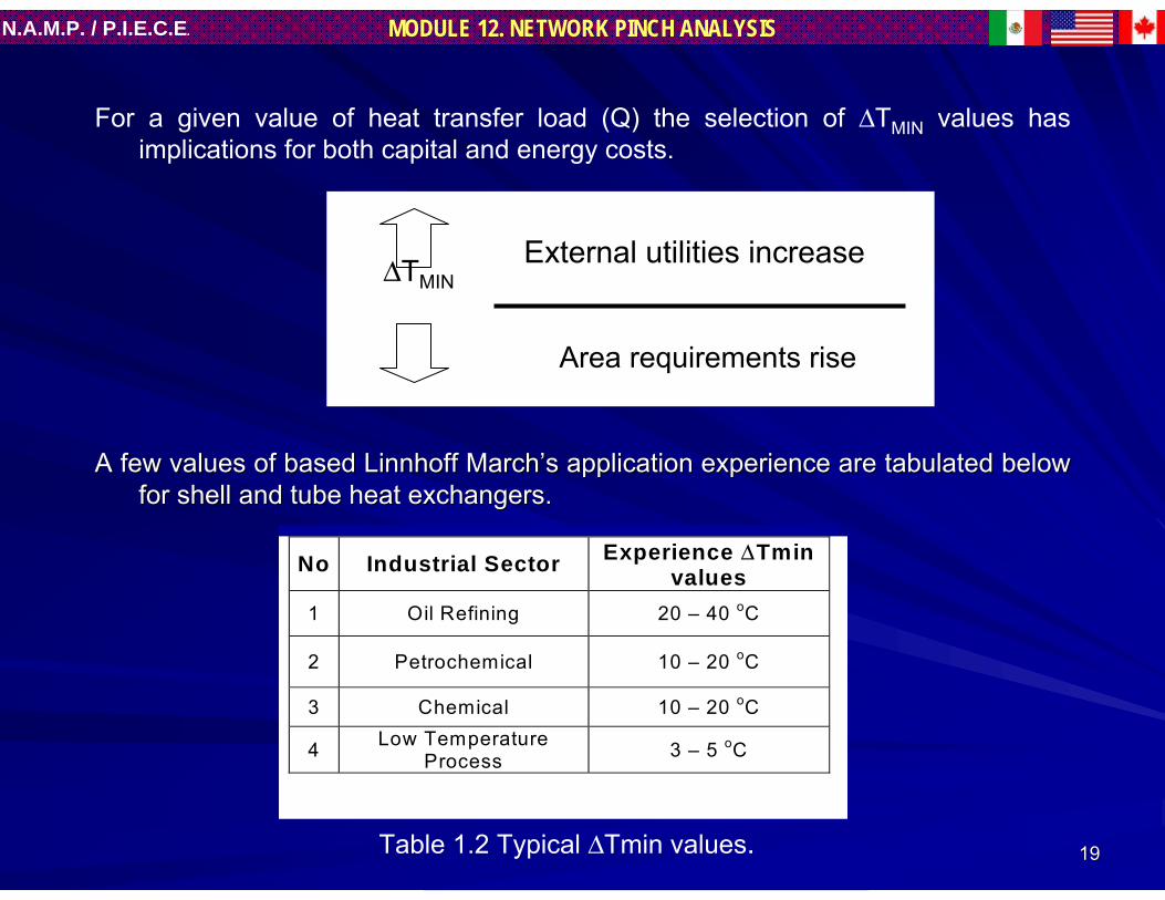
For a given value of heat transfer load (Q) the selection of ΔTMIN values has implications for both capital and energy costs.
ΔTMIN
A few values of based A few values of based LinnhoffLinnhoff MarchMarch’’s application experience are tabulated below s application experience are tabulated below for shell and tube heat exchangers.for shell and tube heat exchangers.
Area requirements rise
External utilities increase
No Industrial Sector Experience ΔTminvalues
1 Oil Refining 20 – 40 oC
2 Petrochemical 10 – 20 oC
3 Chemical 10 – 20 oC
4 Low TemperatureProcess 3 – 5 oC
Table 1.2 Typical ΔTmin values.

2020
MODULE 12. NETWORK PINCH ANALYSISN.A.M.P. / P.I.E.C.E.
4 Construction of Composite Curves and Grand Composite Curve.4 Construction of Composite Curves and Grand Composite Curve.
Composite CurvesComposite CurvesComposite Curves consist of temperature (T) Composite Curves consist of temperature (T) -- Enthalpy (H) profiles of heat Enthalpy (H) profiles of heat availability in the process (the Hot Composite Curve) and heat davailability in the process (the Hot Composite Curve) and heat demands in the emands in the process (the Cold Composite Curve) together in a graphical repreprocess (the Cold Composite Curve) together in a graphical representation.sentation.
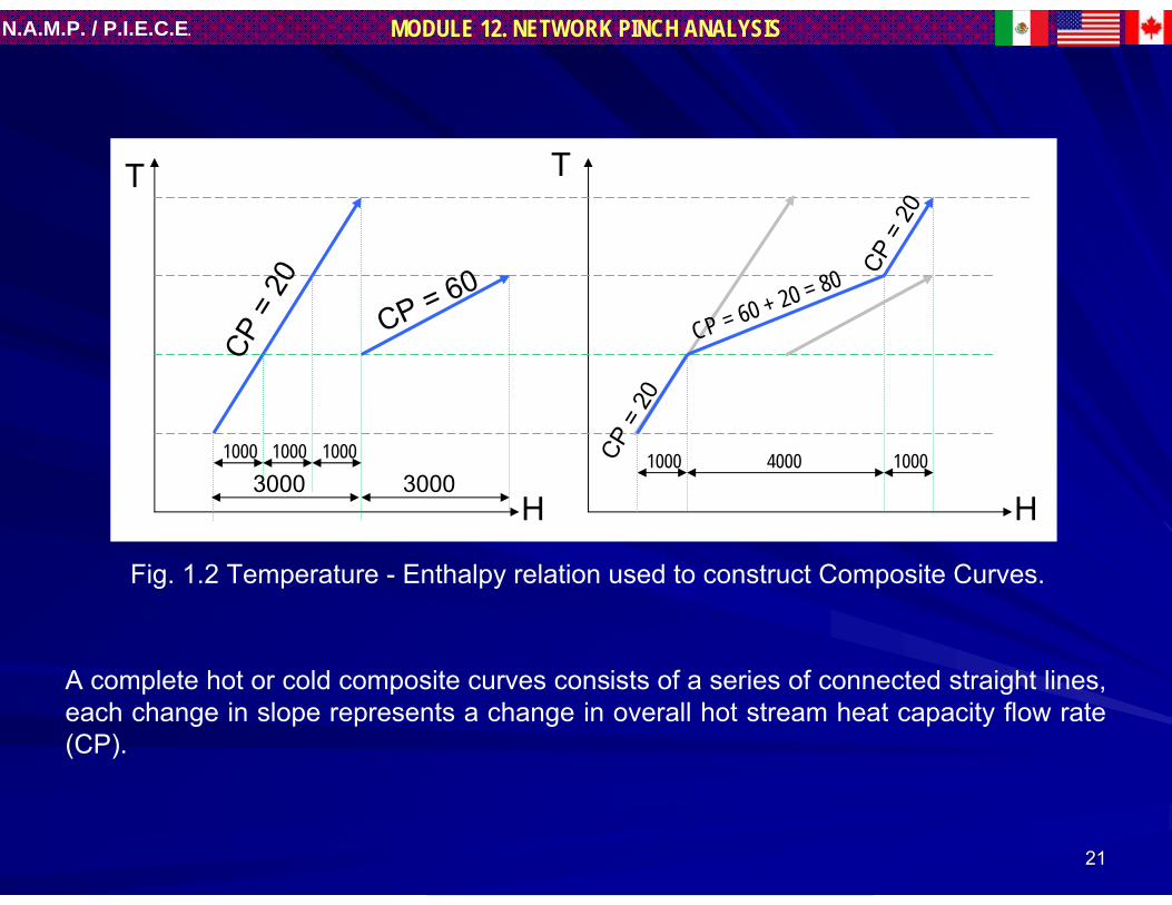
In general any stream with a constant heat capacity (CP) value iIn general any stream with a constant heat capacity (CP) value is represented on a s represented on a diagram by a straight line running from stream supply temperaturdiagram by a straight line running from stream supply temperature to stream target e to stream target temperature. When there are a number of hot and cold composite ctemperature. When there are a number of hot and cold composite curves simply urves simply involves the addition of the enthalpy changes of the stream in tinvolves the addition of the enthalpy changes of the stream in the respective he respective temperature intervals.temperature intervals.
An example of hot composite curves is shown in Fig. 1.2An example of hot composite curves is shown in Fig. 1.2
2121
MODULE 12. NETWORK PINCH ANALYSISN.A.M.P. / P.I.E.C.E.
A complete hot or cold composite curves consists of a series of connected straight lines, each change in slope represents a change in overall hot stream heat capacity flow rate (CP).
T T
H H
CP =
20
CP = 60
3000 300010001000 1000 CP
= 2
0
CP =
20
1000 10004000
Fig. 1.2 Temperature - Enthalpy relation used to construct Composite Curves.
CP = 60 + 20 = 80

2222
MODULE 12. NETWORK PINCH ANALYSISN.A.M.P. / P.I.E.C.E.
Combined Composite Curves.Combined Composite Curves.
Combined Composite Curves are used to predict targets for;– Minimum energy (both hot and cold utility) required.– Minimum network area required, and– Minimum number of exchangers units required.
For heat exchange to occur from the hot stream to the cold stream, the hot stream cooling curve must lie above the cold stream-heating curve.
Because of the “kinked” nature of the composite curves, they approach each other most closely at one point defined as the minimum approach temperature (ΔTMIN).
ΔTMIN can be measured directly from the T-H profiles as being the minimum vertical difference between the hot and cold curves. This point of minimum This point of minimum temperature difference represents a bottleneck in heat recoverytemperature difference represents a bottleneck in heat recovery and is and is commonly referred to as the commonly referred to as the ““PinchPinch””..

2323
MODULE 12. NETWORK PINCH ANALYSISN.A.M.P. / P.I.E.C.E.
ΔΔT min and pinch Point.T min and pinch Point.The The ΔΔTminTmin values determine how closely the hot and cold composite curves values determine how closely the hot and cold composite curves can can be be ““pinchedpinched”” (or (or ““squeezed) without violating the second law of Thermodynamics squeezed) without violating the second law of Thermodynamics (none of the heat exchangers can have a temperature crossover).(none of the heat exchangers can have a temperature crossover).
“PINCH”
QH, MIN
QC,MIN
ΔTMIN
T
H
Fig. 1.3 Energy targets and “the pinch” with Composite Curves.

2424
MODULE 12. NETWORK PINCH ANALYSISN.A.M.P. / P.I.E.C.E.
Process to processHeat Recovery Potential
At a particular ΔTMIN value, the overlap shows the maximum possible scope for heat recovery within the process. The hot end and cold end overshoots indicate minimum hot utility requirement (QH,MIN) and minimum cold utility requirement (QC,MIN), of the process for the chosen ΔTMIN.Thus, the energy requirement for a process is supplied via process to process heat exchange and/or exchange with several utility levels (steam levels, refrigeration levels, hot oil circuit, furnace flue gas, etc.)
Hot Composite Curve
Cold Composite Curve
Hot Utilities
QH, MIN
Cold Utilities
QC, MIN
PINCH
ΔTMIN
Tem
pera
ture
EnthalpyFig. 1.4 Combined Composite Curves.

2525
MODULE 12. NETWORK PINCH ANALYSISN.A.M.P. / P.I.E.C.E.
Problem Table Algorithm for minimum utility calculations.
Graphical constructions are not the most convenient means of determining energy needs. A numerical approach called “Problem Table Algorithm” PTA was developed by Linnhoff & Flower (1978) as a means of determining the utility needs of a process and the location of the process Pinch. The PTA lends itself to hand calculations of the energy targets.
For the problem data from Table 1.3 (Grid representation is shown in Fig. 1.8) streams are shown in a schematic representation with a vertical temperature scale. Temperature interval boundaries are superimposed.
The interval boundary temperatures are set at 1/2 ΔTMIN ( 5oC in this example) below hot stream temperatures and 1/2 ΔTMIN above cold stream temperatures. So for example in interval number 2 in Fig. 1.4, streams 2 and 4 (the hot streams) run from 150 oC to 145 oC, and stream 3 (the cold stream) from 135 oCto 140 oC.
Setting up the intervals in this way guarantees that full heat interchange within any interval is possible. Hence, each interval will have either a net surplus or net deficit of heat as dictated by enthalpy balance, but never both. This is shown in Fig. 1.5.
2626
MODULE 12. NETWORK PINCH ANALYSISN.A.M.P. / P.I.E.C.E.
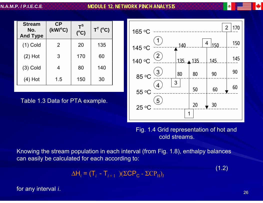
Knowing the stream population in each interval (from Fig. 1.8), enthalpy balances can easily be calculated for each according to:
ΔHi = (Ti - Ti + 1 )(ΣCPC - ΣCPH)I
for any interval i.
165 oC
145 oC
140 oC
85 oC
55 oC
25 oC
1
2
3
4
5
3
1
4
2
140
80
20
135
150
30
170
60
135
50
80
145
90
60
150
145
90
Fig. 1.4 Grid representation of hot and cold streams.
StreamNo.
And Type
CP(kW/oC) TS
(oC) TT (oC)
(1) Cold 2 20 135
(2) Hot 3 170 60
(3) Cold 4 80 140
(4) Hot 1.5 150 30
Table 1.3 Data for PTA example.
(1.2)
2727
MODULE 12. NETWORK PINCH ANALYSISN.A.M.P. / P.I.E.C.E.
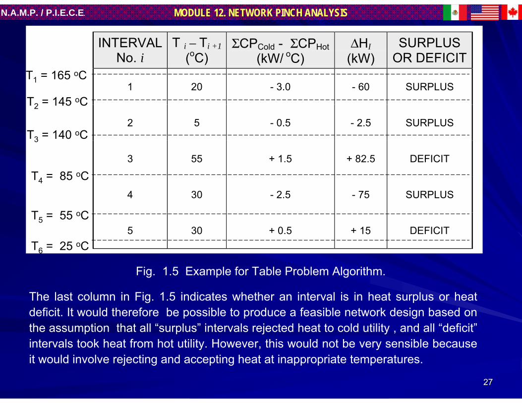
INTERVALNo. i
T i – Ti +1(oC)
ΣCPCold - ΣCPHot(kW/ oC)
ΔHI(kW)
SURPLUSOR DEFICIT
1 20 - 3.0 - 60 SURPLUS
2 5 - 0.5 - 2.5 SURPLUS
3 55 + 1.5 + 82.5 DEFICIT
4 30 - 2.5 - 75 SURPLUS
5 30 + 0.5 + 15 DEFICIT
Fig. 1.5 Example for Table Problem Algorithm.
T1 = 165 oC
T2 = 145 oC
T3 = 140 oC
T4 = 85 oC
T5 = 55 oC
T6 = 25 oC
The last column in Fig. 1.5 indicates whether an interval is in heat surplus or heat deficit. It would therefore be possible to produce a feasible network design based on the assumption that all “surplus” intervals rejected heat to cold utility , and all “deficit”intervals took heat from hot utility. However, this would not be very sensible because it would involve rejecting and accepting heat at inappropriate temperatures.
2828
MODULE 12. NETWORK PINCH ANALYSISN.A.M.P. / P.I.E.C.E.
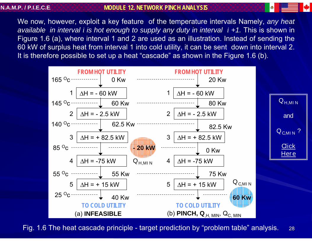
We now, however, exploit a key feature of the temperature intervals Namely, any heat available in interval i is hot enough to supply any duty in interval i +1. This is shown in Figure 1.6 (a), where interval 1 and 2 are used as an illustration. Instead of sending the 60 kW of surplus heat from interval 1 into cold utility, it can be sent down into interval 2. It is therefore possible to set up a heat “cascade” as shown in the Figure 1.6 (b).
Fig. 1.6 The heat cascade principle - target prediction by “problem table” analysis.
QH,MIN
and
QC,MIN ?
Click Here
QH,MIN
QC,MIN
ΔH = - 60 kW
ΔH = - 2.5 kW
ΔH = + 82.5 kW
ΔH = -75 kW
ΔH = + 15 kW
FROM HOT UTILITY165 Oc
145 Oc
140 Oc
85 Oc
55 Oc
25 OcTO COLD UTILITY
1
2
3
4
5
0 Kw
60 Kw
62.5 Kw
55 Kw
40 Kw
ΔH = - 60 kW
ΔH = - 2.5 kW
ΔH = + 82.5 kW
ΔH = -75 kW
ΔH = + 15 kW
FROM HOT UTILITY
TO COLD UTILITY
1
2
3
4
5
20 Kw
80 Kw
82.5 Kw
0 Kw
75 Kw
60 Kw
(a) INFEASIBLE (b) PINCH, Q,H, MIN, QC, MIN
- 20 kW

2929
MODULE 12. NETWORK PINCH ANALYSISN.A.M.P. / P.I.E.C.E.
Assuming that not heat is supplied to the hottest interval (1) from hot utility, then the surplus of 60 kW or surplus heat from interval 1is cascaded into interval 2. There it joins the 2.5 kW surplus from interval 2, making 62.5 kW to cascade into interval 3.
Interval 3 has a 82,5 kW deficit, hence after accepting the 62.5 kW it van be regarded as passing on a 20 kW deficit to interval 4.
Interval 4 has a 75 kW surplus and so passes on a 55 kW surplus to interval 5.
Finally, the 15 kW deficit in interval 5 means that 40 kW is the final cascaded energy to cold utility. This in fact is the net enthalpy balance on the whole problem.
Looking at the heat flows between intervals clearly the negativeflow of 20 kW between intervals 3 and 4 is thermodynamically infeasible. To make this feasible (I.e. equal to zero), 20 kW of heat must be added from hot utility as shown in Figure 1.10 (b), and cascaded right through the system.
Determining QDetermining QH,MINH,MIN ,Q,QC,MINC,MIN and Pinch Point from heat and Pinch Point from heat ““cascadecascade””..
ΔH = - 60 kW
ΔH = - 2.5 kW
ΔH = + 82.5 kW
ΔH = -75 kW
ΔH = + 15 kW
FROM HOT UTILITY
TO COLD UTILITY
1
2
3
4
5
20 Kw
80 Kw
82.5 Kw
0 Kw
75 Kw
60 Kw
Fig. 1.6 (b) (Repeat)PINCH, Q,H, MIN, QC, MIN
The net result of this operation is that the minimum utilities requirements have been predicted, i.e. 20 kW hot and 60 kW cold. Further, the position of the pinch has been located. This is at the 85 0C interval boundary temperature where the heat flow is zero.

3030
MODULE 12. NETWORK PINCH ANALYSISN.A.M.P. / P.I.E.C.E.
Grand Composite Curve (GCC).Grand Composite Curve (GCC).
In selecting utilities to be used, determining utility temperatures, and deciding on utility requirements, the composite curves and PTA are not particularly useful. The introduction of a new tool, the grand Composite Curve (GCC), was introduced in 1982 by Itoh, Shiroko and Umeda. The GCC (Figure 1.7) shows the variation of heat supply and demand within the process. Using this diagram the designer can find which utilities are to be used. The designer’s aim is to maximize the use of cheaper utility levels and minimize the use of expensive utility levels. Low-pressure steam and cooling water are preferred instead of high-pressure steam and refrigeration, respectively.
The information required for the construction of the GCC comes directly from the Table Problem Algorithm. The method involves shifting (along the temperature [y] axis) of the hot composite curve down by 1/2 ΔTMIN and that of cold composite curve up by 1/2 ΔTMIN. The vertical axis on the shifted composite curves shows process interval temperature. In others words, the curves are shifted by subtracting part of the allowed temperature approach from the hot stream temperatures and adding the remaining part of the allowed temperature approach to the cold stream temperatures.

3131
MODULE 12. NETWORK PINCH ANALYSISN.A.M.P. / P.I.E.C.E.
Int e
rva l
tem
per a
ture
EnthalpyQC,MIN
QH,MINSHIFTED
COMPOSITE CURVE
Internal Temp. = ActualTemp. ± 1/2 ΔTmin+ : Cold stream- : Hot stream
GCCH1
TH1
H2TH2
TPinch
C2TC2
C1TC1
Fig. 1.7 Grand Composite Curve.
Figure 1.7 shows that it is not necessary to supply the hot utility at the top temperature level. The GCC indicates that we can supply hot utility over two temperature levels TH1 (HP steam) and TH2 (LP steam). Recall that, when placing utilities in the GCC, intervals, and not actual utility temperatures, should be used. The total minimum hot utility requirement remains the same: QH,MIN = H1 + H2. Similarly, QC,MIN = C1 + C2. The points TH2 and TC2 where the H2 and C2 levels touch the GCC are called the “Utility Pinches”. The shaded green pockets represents the process-to-process heat exchange.

3232
MODULE 12. NETWORK PINCH ANALYSISN.A.M.P. / P.I.E.C.E.
Composite curves give conceptual understanding of Composite curves give conceptual understanding of how energy how energy targets can be obtained.targets can be obtained.
The Problem Table gives the same results (including the The Problem Table gives the same results (including the ““PinchPinch””location) more easily.location) more easily.
Energy targeting is a powerful design and Energy targeting is a powerful design and ““process integrationprocess integration””aid.aid.
SummarizingSummarizing

1.3 Cost Targeting1.3 Cost Targeting
5. Estimation of minimum energy costs.
6. Estimation of Heat Exchanger Network (HEN) Capital Cost Target.
7. Estimation of Optimum ΔTMIN value by Energy-Capital Trade Off.
8. Estimation of Practical Targets for HEN Design.

3434
MODULE 12. NETWORK PINCH ANALYSISN.A.M.P. / P.I.E.C.E.
Once the ΔTMIN is chosen, minimum hot and cold utility requirements can be evaluated from the composite curves. The GCC provides information regarding the utility levels selected to meet QH,MIN and QC,MIN requirements.
If he unit cost of each utility is known, the total energy cost can be calculated using the energy equation given below
TOTAL ENERGY COST = ΣQU·CU
where Qwhere QUU = Duty of utility U, kW= Duty of utility U, kWCCUU = Unit Cost of utility U, $/kW, year= Unit Cost of utility U, $/kW, yearU = Total Number of utilities used. U = Total Number of utilities used.
5. Estimation of minimum energy costs.
(1.3)

3535
MODULE 12. NETWORK PINCH ANALYSISN.A.M.P. / P.I.E.C.E.
The capital cost of a heat exchanger network is dependent upon three factors:1 the number of exchanger2 the overall network area3 the distribution of area between the exchangersPinch analysis enable targets for the overall heat transfer area and minimum
number units of a heat exchanger network (HEN) to be predicted prior to detailed design. It is assumed that the area is evenly distributed between the units. The area distribution cannot be predicted ahead of design.
Area targetingArea targetingThe calculation of surface area for a single counter-current heat exchanger requires the knowledge of the temperatures of the stream in and out (TLM I.e. Log Mean Temperature Difference or LMTD), overall heat transfer coefficient (U-value), and total heat transferred (Q). The area is given by the relation
Area = Q / U x TLM
6 Estimation of Heat Exchanger Network (HEN) Capital Cost Target.
(1.4)

3636
MODULE 12. NETWORK PINCH ANALYSISN.A.M.P. / P.I.E.C.E.
The composite curves can be divided into a set of adjoining enthalpy intervals such that within each interval , the hot and cold composite do not change slope. Here the heat exchange is assumed to be “vertical” (pure counter-current heat exchange). The hot streams in any enthalpy interval, at any point, exchanges heat with the cold streams at the temperature vertically below it. The total area of the HEN (AMIN) is given by the equation following
HEN AREAMIN = A1 + A2 + A3 +……+ Ai =Σ [ (1/ΔTLM) Σqj/hj]
where i denotes the ith enthalpy and interval j denotes jth stream, TLM denotes LMTD in the ith interval, and A1 + A2 + A3 +……+ Ai is shown in the Figure 1.8
i j
Fig. 1. 8 HEN AreaMIN estimation fromcomposite curves.
(1.5)
A1
A2
A3
A4
A5
EnthalpyIntervals
H
T

3737
MODULE 12. NETWORK PINCH ANALYSISN.A.M.P. / P.I.E.C.E.
Number of Units targeting.Number of Units targeting.
For the minimum number of heat exchanger units (NMIN) required for MER (Minimum Energy Requirements or Maximum Energy Recovery), the HEN can be evaluated prior to HEN design by using a simplified form of Euler’s graph theorem. In designing for the minimum energy requirement (MER), not heat transfer is allowed across the Pinch and so a realistic target for the minimum number of units (NMIN MER) is the sum of the targets evaluated both above and below the pinch separately.
NMIN, MER = [Nh + NC + NU - 1]AP + [Nh + NC + NU - 1]BP
where where NNHH = Number of hot streams= Number of hot streamsNNCC = Number of cold streams= Number of cold streamsNNUU = Number of utility streams= Number of utility streamsAP / BP : Above Pinch / Below Pinch: Above Pinch / Below Pinch
..
The actual HEN Total Area required is generally within 10% of the area target as calculated by Eq, (1.5). With inclusion of temperature correction factors area targeting can be extended to non counter-current heat exchange as well.
(1.6)

3838
MODULE 12. NETWORK PINCH ANALYSISN.A.M.P. / P.I.E.C.E.
HEN total capital cost targetingHEN total capital cost targeting..The target for the minimum surface area (AMIN) and the number of units (NMIN) can
be combined together with the heat exchanger cost law to determine the targets for HEN capital cost (CHEN). The capital cost is annualized using an annualization factor that takes into account interest payments on borrowed capital. The equation used for calculation the total capital cost and exchanger cost law is given in equation 1.6.
C($)HEN = [NMIN {a + b(AMIN / NMIN )C}]AP + [NMIN {a + b(AMIN / NMIN )C}]BP
where a,b and c are constants in exchanger cost law
Exchanger cost ($) = a + b (Area)c
For the Exchanger Cost Equation shown above, typical values for a carbon steel shell and tube exchanger would be: a = 16,000, b = 3,200 and c = 0.7 . The installed cost can be considered to be 3.5 times the purchased cost given by the Exchanger Cost equation.
(1.7)

3939
MODULE 12. NETWORK PINCH ANALYSISN.A.M.P. / P.I.E.C.E.
Total Cost targeting.Total Cost targeting.Used to determine the optimum level of heat recovery or the optimum ΔTMIN value,
by balancing energy and capital costs. Using this method it is possible to obtain an accurate estimate (within 10 - 15 %) of overall heat recovery system costs without having to design the system. The essence of the pinch approach is the speed of economic evaluation.

4040
MODULE 12. NETWORK PINCH ANALYSISN.A.M.P. / P.I.E.C.E.
7. Estimation of Optimum ΔTMIN value by Energy-Capital Trade Off.
To arrive at an optimum value, the total annual cost (the sum of total annual energy and capital cost) is plotted at varying ΔTMIN values (Figure 1.9). Three key observation can be made from Figure 1.9:
1 An increase in ΔTMIN values result in higher energy cost and lower capital costs.2 An decrease in ΔTMIN values result in lower energy costs and higher capital
costs.3 An optimum ΔTMIN exists where the total annual cost of energy and capital
costs is minimized.
Fig. 1.9 Energy-capital cost trade off (optimum ΔTMIN)
Total Cost
Energy Cost
Capital Cost
Ann
uali z
ed C
ost
ΔTMIN
Optimum ΔTMIN
By systematically varying the temperature approach we can determine the optimum heat recovery or the ΔTmin for the process

4141
MODULE 12. NETWORK PINCH ANALYSISN.A.M.P. / P.I.E.C.E.
8. Estimation of Practical Targets for HEN Design.
The heat exchanger network designed on the basis of the estimated optimum ΔTMIN value is not always the most appropriate design. A very small ΔTMINvalue, perhaps 8oC, can lead to a very complicated network design with a large total area due to low driving forces. The designer in practice, select a higher value (15 oC) and calculates the marginal increase in utility duties and area requirements. If the marginal cost increase is small, the higher value of ΔTMINvalue is selected as the practical pinch point for the HEN design.
Recognizing the significance of the pinch temperature allows energy targets to be realized by design of appropriate heat recovery network.
So what is the significance of the pinch temperature?
The pinch divide the process into two separate systems each of which is in enthalpy balance with the utility. The pinch point is unique for each process. Above the pinch, only the hot utility is required. Below the pinch, only the cold utility is required. Hence, for an optimum deign, no heat should be transferred across the pinch. This is known as the key concept in Pinch Technology.
4242
MODULE 12. NETWORK PINCH ANALYSISN.A.M.P. / P.I.E.C.E.
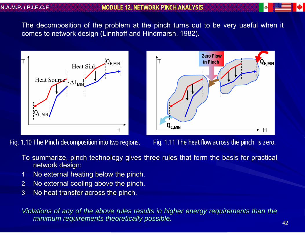
To summarize, pinch technology gives three rules that form the bTo summarize, pinch technology gives three rules that form the basis for practical asis for practical network design:network design:
11 No external heating below the pinch.No external heating below the pinch.22 No external cooling above the pinch.No external cooling above the pinch.33 No heat transfer across the pinch.No heat transfer across the pinch.
Violations of any of the above rules results in higher energy reViolations of any of the above rules results in higher energy requirements than the quirements than the minimum requirements theoretically possible.minimum requirements theoretically possible.
The decomposition of the problem at the pinch turns out to be very useful when it comes to network design (Linnhoff and Hindmarsh, 1982).
ΔTMIN
QH,MIN
QC,MIN
T
H
Fig. 1.10 The Pinch decomposition into two regions.
Heat Sink
Heat Source
QH,MIN
QC,MIN
T
H
Fig. 1.11 The heat flow across the pinch is zero.
Zero Flowin Pinch

1.4 Heat Exchange Network (HEN) 1.4 Heat Exchange Network (HEN) DesignDesign
9. Design of Heat Exchanger Network.
9.1 Network Representation.9.2 Design for the Best Energy Recovery.9.3 Complete Design.

4444
MODULE 12. NETWORK PINCH ANALYSISN.A.M.P. / P.I.E.C.E.
9. Design of Heat Exchanger Network.
9.1 Network Representation.The graphical method of representing flow streams and heat recovery matches is called “Grid Diagram”. In order to describe this graphical method consider the simple example below.The heat exchanger network from the flowsheet in Figure 1.12 can be represented in the “grid” form at Figure 1.13 introduced by Linnhoff and Flower (1982)
Reactor
Sep. Drum
1
2
Steam140 oC 200 oC
120 oC100 oC 200 oC30 oC
25 oCFeed 170 oC
100 oC30 oC
CoolingCrude Product
Fig. 1.12 Heat exchanger network in the flowsheet representation.

4545
MODULE 12. NETWORK PINCH ANALYSISN.A.M.P. / P.I.E.C.E.
The advantage of this representation is that the heat exchange matches 1 and 2 (each represented by two circles joined by a vertical line in the grid) can be placed in either order without redrawing the stream system.
In flowsheet representation, if it were desired to match recycle against the hottest part of the reactor effluent, the stream layout would have to be redrawn. Also, the grid represent the countercurrent nature of the heat exchange, making it easier to check exchanger temperature feasibility.
Finally the pinch is easily represented in the grid, whereas it cannot be represented on the flowsheet.
REACTOREFLUENT
170 oC 120 oC 100 oC 30 oC
H
H
C1
1
2
2
200 oC
200 oC
140 oC
100 oC 30 oC
25 oC FEED
RECYCLE
Fig. 1.13 Heat exchanger network in the Grid representation.

4646
MODULE 12. NETWORK PINCH ANALYSISN.A.M.P. / P.I.E.C.E.
9.2 Design for the Best Energy Recovery9.2 Design for the Best Energy Recovery
The data in Table 1.3 were analyzed by the Problem Table method in sub-section 4.3 with the result that the minimum utility requirements are 20 kW hot and 60 kW cold. The pinch occurs where the hot streams are at 90 oC and the cold at 80 oC. The grid structure for the problem is shown in Figure 1.14, with the pinch represented as a vertical dotted line.
Above the pinchAbove the pinch:: the hot streams are cooled from their supply temperatures to their pinch temperature, and the cold streams heated from their pinch temperatures to their target temperatures.
Below the pinchBelow the pinch: : the position is reversed with hot streams being cooled from the pinch to target temperatures and cold streams being heated from supply to pinch temperature.
2
4
1
3
170 oC 90 oC 90 oC 60 oC
150 oC
135 oC
140 oC
90 oC 90 oC
80 oC
80 oC
80 oC
30 oC
20 oC
PINCHQH,MIN = 20 kW QC,MIN = 60 kW
CP (kW/oC)3.0
1.5
2.0
4.0
Fig. 1.14 Example problem stream data, showing Pinch.

4747
MODULE 12. NETWORK PINCH ANALYSISN.A.M.P. / P.I.E.C.E.
Above the pinch all streams must be brought to pinch temperature by interchange against cold streams. We must therefore start the design at the pinch, finding matches that fulfil this condition.
DESIGN ABOVE THE PINCH. DESIGN ABOVE THE PINCH. In this example, above the pinch there are two hot streams at pinch temperature,
therefore requiring two “pinch matches”. In Figure 1.15 a match between streams 2 and 1 is shown, with a T/H plot of the match shown in inset. (Note that the stream directions have been reversed so as to mirror the directions in the grid representation).
2
4
QH,MIN = 20 kW
1
3
3.0
1.5
2.0
4.0
CP (kW/oC)
ΔTMIN
Fig. 1.15 Example problem hot end design. Infeasible.
Because the CP of stream 2 is grater than that of stream 1, as soon as any load is placed on the match, the ΔT in the exchanger becomes less than ΔT MIN at its hot end. The exchanger is clearly infeasible and therefore we must look for another match.
T
H
Infeasible !!

4848
MODULE 12. NETWORK PINCH ANALYSISN.A.M.P. / P.I.E.C.E.
In Figure 1.16, streams 2 and 3 are matched, and now the relative gradients of the T/ H plots mean that putting load on the exchanger opens up the ΔT.
2
4
QH,MIN = 20 kW
1
3
3.0
1.5
2.0
4.0
CP (kW/oC)
ΔTMINΔTMIN
T T
H H
Fig. 1.16 Example problem hot end design. Acceptable.
This match is therefore acceptable. If it is put in as a firm design decision, then stream 4 must be brought to pinch temperature by matching against stream 1. Looking at the relatives sizes of the CPs for streams 4 and 1, the match is feasible (CP4 < CP1).There are no more streams requiring cooling to pinch temperature and so we have found a feasible pinch design because only two pinch matches are required.
In design immediately above the pinch, it is required to meet the criterion:CPHOT ≤ CPCOLD

4949
MODULE 12. NETWORK PINCH ANALYSISN.A.M.P. / P.I.E.C.E.
Maximize Exchanger Loads.Maximize Exchanger Loads.Having found a feasible pinch design it is necessary to decide on the match heat loads. The recommendation is “maximize the heat load so as to completely satisfy one of the streams”. This ensures minimum number of units employed.
2
4
170 oC 90 oC
150 oC
135 oC
140 oC
90 oC
80 oC
80 oCH 125 oC
240 kW
90 kW20 kW1
3
3.0
1.5
2.0
4.0
CP (kW/oC)
Fig. 1.17 Example problem hot end design.Maximizing exchanger loads.
In the example problem, since stream 2 above the pinch requires 240 kW of cooling and stream 3 above the pinch requires 240 kW of heating, co-incidentally the 2/3 match is capable of satisfying both streams. However, the 4/1 match can only satisfy stream 4, having a load of 90 kW and therefore heating up stream 1 only as far as 125 oC. Since, both hot streams have now have been completely exhausted by these two design steps, stream 1 must be heated from 125 oC to its target temperature of 135 oC by external hot utility as shown in Figure 1. 17.

5050
MODULE 12. NETWORK PINCH ANALYSISN.A.M.P. / P.I.E.C.E.
DESIGN BELOW THE PINCH.DESIGN BELOW THE PINCH.The “above the pinch” section has been designed independently of the “below the pinch”
section, and not using utility above the pinch. Below the pinch the design steps follow the same philosophy, only with the design criterion that mirror those for the “above the pinch” design.
Now, it is required to bring cold streams to pinch temperature by interchange with hot streams, since we do not want to use utility heating below the pinch (Figure 1.18).
In this example, only one cold stream exist below the pinch which must be matched against one of the two available hot streams. The match between streams 1 and 2 is feasible because the CP of the hot stream is greater than of the cold. The other possible match (stream 1 with stream 4) is not feasible.
1
CP (kW/oC)3.0
1.5
2.0
2
4ΔTMIN
Infeasible!!,Why?
Feasible
Fig. 1.18 Example problem cold design. 2/1 Match acceptable, 2/4 match infeasible.
T
H
Immediately below the pinch, the necessary criterion is: CPHOT ≥ CPCOLD …. which is inverse of the criterion for design immediately above the pinch.
5151
MODULE 12. NETWORK PINCH ANALYSISN.A.M.P. / P.I.E.C.E.
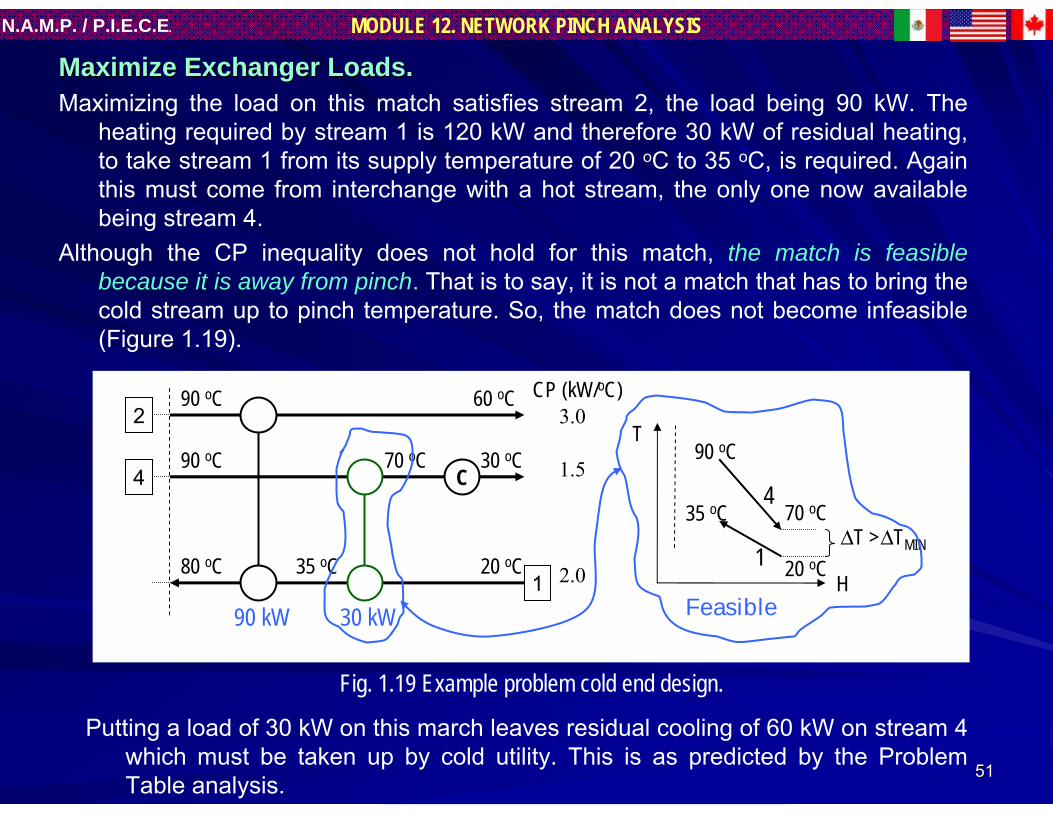
Maximize Exchanger Loads.Maximize Exchanger Loads.Maximizing the load on this match satisfies stream 2, the load being 90 kW. The
heating required by stream 1 is 120 kW and therefore 30 kW of residual heating, to take stream 1 from its supply temperature of 20 oC to 35 oC, is required. Again this must come from interchange with a hot stream, the only one now available being stream 4.
Although the CP inequality does not hold for this match, the match is feasible because it is away from pinch. That is to say, it is not a match that has to bring the cold stream up to pinch temperature. So, the match does not become infeasible (Figure 1.19).
1
CP (kW/oC)3.0
1.5
2.0
2
4
ΔTMIN
Feasible
70 oC
20 oCΔT >
90 oC
35 oC
T
H
90 oC
90 oC
80 oC 35 oC 20 oC
70 oC
60 oC
C30 oC
4
1
90 kW 30 kW
Fig. 1.19 Example problem cold end design.
Putting a load of 30 kW on this march leaves residual cooling of 60 kW on stream 4 which must be taken up by cold utility. This is as predicted by the Problem Table analysis.

5252
MODULE 12. NETWORK PINCH ANALYSISN.A.M.P. / P.I.E.C.E.
9.3 Complete Design.9.3 Complete Design.
Putting the “hot end” and “cold end” designs together gives the completed design (Figure 1.20). It achieves best possible energy performance for a ΔTMIN of 10 oCincorporating four exchangers, one heater and one cooler. In other words, six units of heat transfer equipment in all.
4
2
1
3
170 oC 60 oC
150 oC 30 oC
135 oC 20 oC
140 oC 80 oC
125 oC
1
240 kW
90 oC
90 oC2
90 kW
80 oC
3
90 kW
35 oC
70 oC4
30 kW
3.0
1.5
2.0
4.0
CP (kW / oC)
Fig. 1.20 Example problem completed design.
C60 kW
H20 kW

5353
MODULE 12. NETWORK PINCH ANALYSISN.A.M.P. / P.I.E.C.E.
Summarizing:Summarizing:
Dividing the problem at the pinch, and designing each part separDividing the problem at the pinch, and designing each part separately.ately.
Starting the design at the pinch and moving away.Starting the design at the pinch and moving away.
Immediately adjacent to the pinch, obeying the constraints:Immediately adjacent to the pinch, obeying the constraints:
CPCPHOTHOT ≤≤ CPCPCOLDCOLD (Above).(Above).
CPCPHOTHOT ≥≥ CPCPCOLDCOLD (Below).(Below).
Maximizing exchanger loads.Maximizing exchanger loads.
Supplying external heating only above the pinch, and external coSupplying external heating only above the pinch, and external cooling only oling only below the pinch.below the pinch.
These are the basic elements oh the These are the basic elements oh the ““Pinch Design MethodPinch Design Method”” of of LinnhoffLinnhoffand and HindmarshHindmarsh (1982).(1982).

5454
MODULE 12. NETWORK PINCH ANALYSISN.A.M.P. / P.I.E.C.E.
Summarizing steps for Summarizing steps for HENsHENs design:design:
4 Construction ofComposite and Grand Composite curves
1 Identification of hot, cold and utility streamsin the process.
2 Thermal data Extraction for process and utility streams
3 Selection of initialΔTMIN value
5 Estimation of minimumenergy cost targets
6 Estimation of HENcapital cost targets
7 Estimation of optimumΔTMIN value
8 Estimation of practical targets for HEN design
9 Design of heatexchanger network(HEN)
5555
MODULE 12. NETWORK PINCH ANALYSISN.A.M.P. / P.I.E.C.E.
TIER I: FUNDAMENTALSTIER I: FUNDAMENTALS
1.1. HEAT RECOVERY NETWORKS (HEN).HEAT RECOVERY NETWORKS (HEN).2.2. STEADY STATE SIMULATION of STEADY STATE SIMULATION of HENsHENs..3.3. OPERABILITY ANALYSIS of OPERABILITY ANALYSIS of HENsHENs..4.4. RETROFIT of RETROFIT of HENsHENs..5.5. MASSS EXCHANGE NETWORKS (MEN).MASSS EXCHANGE NETWORKS (MEN).6.6. OPERABILITY ANALYSIS of OPERABILITY ANALYSIS of MENsMENs..

5656
MODULE 12. NETWORK PINCH ANALYSISN.A.M.P. / P.I.E.C.E.
2.2. STEADY STATE SIMULATION of STEADY STATE SIMULATION of HENsHENs..
2.1 Introduction2.1 Introduction2.2 Response equations.2.2 Response equations.2.3 Modeling the thermal performance of 2.3 Modeling the thermal performance of HENsHENs..

5757
MODULE 12. NETWORK PINCH ANALYSISN.A.M.P. / P.I.E.C.E.
2.1 Introduction2.1 Introduction..Flexible Network:Flexible Network:For an existing heat recovery network to maintain its target temperatures when changed
operating conditions come into being is very significant to avoid bottlenecks at individual heat exchangers.
Typical de-bottlenecking practices for heat exchangers include modifications to surface area (overdesign) and to heat transfer coefficients (use of bypass).
If the modified operating conditions return to their original condition after a network has been de-bottlenecked, new disturbances are produced and the network has to be de-bottlenecked again in order to achieve the specified target temperatures.
A Flexible Network is one that is capable to providing an acceptable performance after being subjected to those two de-bottlenecking stages..

5858
MODULE 12. NETWORK PINCH ANALYSISN.A.M.P. / P.I.E.C.E.
Steady State ResponseSteady State Response
During a process design the engineer fixes important parameters such as reactor feed and operating temperature, distillation column pre-heat levels, reflux ratios etc. However, individual equipment items are often able to operate efficiently over quite a large range of conditions. For instance, in many cases a reduction in reactor operating temperature of a few degrees will have a minimal effect on conversion and selectivity.
The first step in analyzing the flexibility requirements of heatThe first step in analyzing the flexibility requirements of heat recovery networks is the recovery networks is the specification of the process temperatures bounds, also called specification of the process temperatures bounds, also called ““acceptable boundsacceptable bounds””. . These indicate the temperature range over which the process can These indicate the temperature range over which the process can still operate. still operate.
Tem
pera
ture
Flow
rate
time
Upper Bound
Upper Bound
Lower Bound
Lower Bound
Fig. 2.1 Acceptable Bounds
A heat exchanger network is supposed to have the required flexibility if its steady state response to a combination of inlet temperature and flow ratedisturbances is within the acceptable bounds.

5959
MODULE 12. NETWORK PINCH ANALYSISN.A.M.P. / P.I.E.C.E.
Propagation of disturbances through networks.Propagation of disturbances through networks.The propagation of disturbances through heat recovery networks takes place by
traveling down stream and through heat exchangers.
1
2
3
4
5
E3
E1
E2E4
C
C
D
D
D Disturbance
C Control Objective
The effect of the disturbances on target temperatures can be assessed by determining the steady state response of the network. This steady state response can be used to implement retrofit strategies that will lead to flexible systems able to cater for seasonal or temporary variations in operating conditions
Fig. 2.2 propagation of disturbances through networks.

6060
MODULE 12. NETWORK PINCH ANALYSISN.A.M.P. / P.I.E.C.E.
2.2 Response equations2.2 Response equationsExchanger thermal effectivenessExchanger thermal effectiveness..
The response of individual exchangers to changes in flow rate and inlet temperatures can be assessed quickly and accurately by the use of the thermal effectiveness (ε ) relations.
Exchanger Thermal Effectiveness, represents the ratio of the actual heat load to the maximum load that is thermodynamically possible.
From this definition it can be shown that the exchanger thermal effectiveness can be represented by the ratio of temperature difference that the CPmin stream undergoes, to the maximum temperature driving force that exists in the exchanger (Fig. 2.3).
31
21
TTTT
−−=ε
Hot
Cold
T1T2
T3 T4
T
H
T1
T2
T3
T4
(2.1) Fig. 2.3 Temperature profiles of a heat Exchanger Where the hot stream is theCPmin stream.

6161
MODULE 12. NETWORK PINCH ANALYSISN.A.M.P. / P.I.E.C.E.
Number of Heat transfer Units (NTU).Number of Heat transfer Units (NTU).The number of transfer units is expressed by
where U is the overall heat transfer coefficient, and A is the exchanger surface area.
InterInter--relation: relation: εε, NTU, C, NTU, C** and flow arrangement.and flow arrangement.Exchanger thermal effectiveness can also be expressed as a function of C* (C* =
CPmin/CPmax), the number of heat transfer units (NTU) and the exchanger flow arrangement. For instance, the expression for a shell and tube exchanger is:
minCPUANTU = (2.2)
( ) ( )( )( ) ⎥
⎥⎦
⎤
⎢⎢⎣
⎡
−
++++
=
+−
+−
2/12*
2/12*
1
12/12**
1
111
2
CNTU
CNTU
e
eCC
ε(2.3)
6262
MODULE 12. NETWORK PINCH ANALYSISN.A.M.P. / P.I.E.C.E.
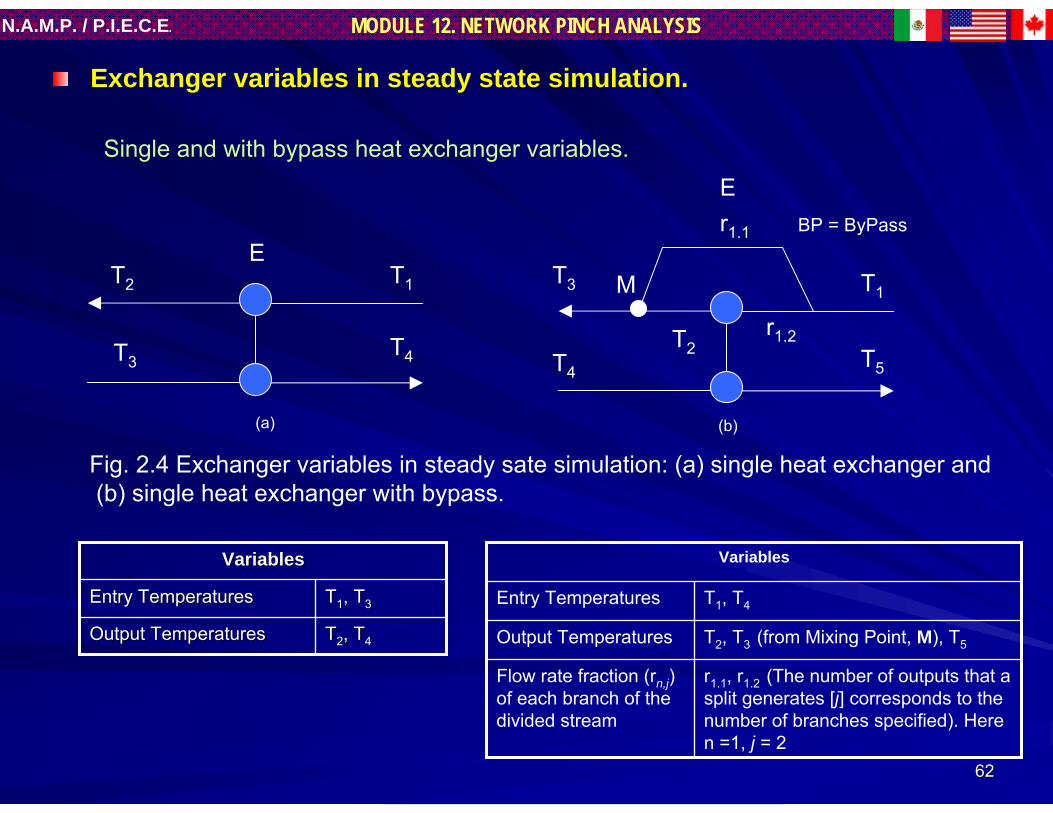
Exchanger variables in steady state simulation.Exchanger variables in steady state simulation.
Single and with bypass heat exchanger variables.
TT22, T, T44Output TemperaturesOutput Temperatures
TT11, T, T33Entry TemperaturesEntry Temperatures
VariablesVariables
ET2 T1
T3T4
Fig. 2.4 Exchanger variables in steady sate simulation: (a) single heat exchanger and(b) single heat exchanger with bypass.
E
T2
T1T3
T4
BP = ByPassr1.1
M
T5
r1.2
r1.1, r1.2 (The number of outputs that a split generates [j] corresponds to the number of branches specified). Here n =1, j = 2
Flow rate fraction (rn,j) of each branch of the divided stream
T2, T3 (from Mixing Point, M), T5Output Temperatures
T1, T4Entry Temperatures
Variables
(a) (b)

6363
MODULE 12. NETWORK PINCH ANALYSISN.A.M.P. / P.I.E.C.E.
Total number of variables in a network (NV).Total number of variables in a network (NV).From the ongoing discussion it can be shown that the total number of temperature and
flow fraction variables (NV) in a network can be determined by
where S the number of process streams. For the exchanger in Fig. 2.4b
Total number of equations in a network.Total number of equations in a network.For a system to be fully defined, the number of variables must be equal to the number of
equations. In the case of an existing heat exchanger network, the equations that can be written are:
a) The thermal effectiveness equation and the heat balance equation for every heat exchanger.From the thermal effectiveness equation Eq. (2.1), the outlet temperature of the CPmin stream in the case of Fig. 3.3b can be expressed as
Combining Eq. (2.5) with the heat balance equation about the exchanger, the outlet temperature of the CPmaxstream can be expressed as
BPMESNV 22 +++=
7)1(21)1(22 =+++=NV
( )4112 TTTT −−= ε
(2.4)
(2.5)
)( 4145 TTCTT −+= ε (2.6)

6464
MODULE 12. NETWORK PINCH ANALYSISN.A.M.P. / P.I.E.C.E.
b)b) The mass balance equation about every mixing point.The mass balance equation about every mixing point.The mass balance equation about any mixing point can be expressed as
where n is the stream number. This equation can be rewritten as
where r is the stream branch flow fraction and
For a bypass j = 2, and at least one flow fraction (r) is known.
c) The heat balance about every mixing point.c) The heat balance about every mixing point.For the exchanger in Fig. 2.4b the equation of heat balance about mixing point can be written as
Where H is the stream enthalpy content. For a given reference state (Tref.) the enthalpy content can be expressed as
∑ =j
Totalnjn mm1
,, && (2.7)
∑ =j
jnr1
, 1 (2.8)
Totaln
jnjn m
mr
,
,, &
&= (2.9)
123 HHH +=
( )refTTCpmH −= &
T2
T1T3
T4
BP r1.1
M
T5
r1.2
Fig. 2.4b
(2.10)
(2.11)

6565
MODULE 12. NETWORK PINCH ANALYSISN.A.M.P. / P.I.E.C.E.
Now the mass balance about the mixing point is
Applying Eq. (2.11) to the various streams at the mixing point, and combining with Eqs. (2.10) and (2.12) and rearranging gives
where r1,1 and r1,2 are the flow fractions of stream 1 in branches 1 and 2.
d.d. The stream supply temperatures which are known.The stream supply temperatures which are known.
e.e. The The jj--1 1 flow fractions at every split point that are known.flow fractions at every split point that are known.
Solution of system of equations.Solution of system of equations.In an existing network, all stream supply temperatures, mass flow rates and exchanger
effectiveness are known.The simultaneous solution of the system of equations permits the calculation of ALL
NETWORK TEMPERATURES.Variations in supply temperatures and flow rates can be readily assessed in order to
obtain the steady state response of the network.
123 mmm &&& += (2.12)
22,111,13 TrTrT += (2.13)

6666
MODULE 12. NETWORK PINCH ANALYSISN.A.M.P. / P.I.E.C.E.
Example 1.Example 1. Simultaneous solution of system equations in a single heat Simultaneous solution of system equations in a single heat exchangerexchanger ..
Taking into consideration the heat exchanger shown in the Fig. Taking into consideration the heat exchanger shown in the Fig. 2.4 a, it can see from effectiveness equations that outlet 2.4 a, it can see from effectiveness equations that outlet temperature for temperature for CPminCPmin streams is:streams is:
and the second equations required come from heat balance and the second equations required come from heat balance about exchanger and it can written asabout exchanger and it can written as
Combining two equations preceding it can obtained a equation Combining two equations preceding it can obtained a equation to outlet temperature for to outlet temperature for CPmaxCPmax stream (Tstream (T44):):
( ) 312 1 TTT εε +−=
E
T
H
T1
T2
T3
T4
Hot
Cold
T1T2
T3 T4
T1
T2
T3
T4
max34min21 )()( CPTTCPTT −=−
314 )1( TCTCT εε −+=
6767
MODULE 12. NETWORK PINCH ANALYSISN.A.M.P. / P.I.E.C.E.
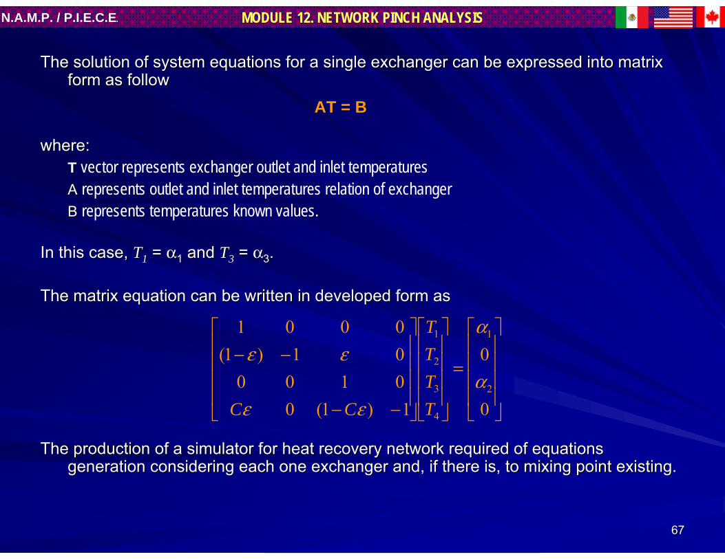
The solution of system equations for a single exchanger can be eThe solution of system equations for a single exchanger can be expressed into matrix xpressed into matrix form as followform as follow
where:where:TT vector represents exchanger outlet and inlet temperaturesAA represents outlet and inlet temperatures relation of exchangerB B represents temperatures known values.
In this case, In this case, TT11 = = αα11 and and TT33 = = αα33..
The matrix equation can be written in developed form asThe matrix equation can be written in developed form as
The production of a simulator for heat recovery network requiredThe production of a simulator for heat recovery network required of equations of equations generation considering each one exchanger and, if there is, to mgeneration considering each one exchanger and, if there is, to mixing point existing.ixing point existing.
AT = B
⎥⎥⎥⎥
⎦
⎤
⎢⎢⎢⎢
⎣
⎡
=
⎥⎥⎥⎥
⎦
⎤
⎢⎢⎢⎢
⎣
⎡
⎥⎥⎥⎥
⎦
⎤
⎢⎢⎢⎢
⎣
⎡
−−
−−
0
0
1)1(0010001)1(0001
2
1
4
3
2
1
α
α
εε
εε
TTTT
CC

6868
MODULE 12. NETWORK PINCH ANALYSISN.A.M.P. / P.I.E.C.E.
Example 1. Example 1. Temperature and flow fraction variables in a heat network.Temperature and flow fraction variables in a heat network.
Total number of variables:Applying Eq. 2.4: NV = S + 2E + M + 2 BP. In this example: S = 4, E = 4, M = 1 and BP = 1, NV = 4 + 2(4) + 1 +2(1)
1
2
3
4
T1T2
T3T4T5T6
T7 T8
T9 T10
T11
T12T13r4,1
r4,2
Equations:- The four stream supply Temperatures are known giving 4
equations.- Two equations can be written for every heat exchanger: the heat
balance and the thermal effectiveness giving another 8 equations.
- The mass balance about the stream split gives 1 equation.- The j-1 known flow fraction gives 1 equation.- The mass balance about the mixing point gives 1 equation.
15 EQUATIONS ARE REQUIRED TO SOLVE THE SYSTEM.The simultaneous solution of this system of equations permits the calculation of all network
temperatures.
Fig. 2.5 Variables in a heat exchange network
6969
MODULE 12. NETWORK PINCH ANALYSISN.A.M.P. / P.I.E.C.E.
Updating exchanger effectiveness and number of transfer unitUpdating exchanger effectiveness and number of transfer units.s.
The influence of temperatures variations on thermal effectiveness is negligible, thus this parameter remains constant when temperature disturbances enter the system.
However, when flow rate variations occur, they change the stream heat coefficient that modifies the overall heat transfer coefficient which in turn affects the number of transfer units, thus causing the thermal effectiveness to change.
In order to account for the change in exchanger effectiveness due to flow rate variations, the individual heat transfer coefficients must be updated.

7070
MODULE 12. NETWORK PINCH ANALYSISN.A.M.P. / P.I.E.C.E.
For the case of shell and tube exchangers operating in turbulent flow, the heat transfer coefficients (h) can be calculated from the following expressions:
Tube side
2.03/2023.0 −− ⋅⋅⋅⋅= RePrGCphtube
or
2.0
3/22.0023.0
TT D
PrCpK−⋅⋅⋅= μ
8.0)(GKh Ttube =
AcmG&
=
where
and
For the original condition (O) and new condition (N), the tube side heat transfer coefficient is
)( 8.0OT
NTube GKh =
The combination of Eqs. (2.18) – (2.19) gives
OTubeO
Tube
NTubeN
Tube hmmh
8.0
⎟⎟⎠
⎞⎜⎜⎝
⎛=
&
&
8.0)( NT
OTube GKh =
Eq. (2.20) allows the heat transfer coefficient to be updated as the stream flow rate changes in the tube side provided turbulent flow remains.
(2.14)
(2.15)
(2.16) (2.17)
(2.18) (2.19)
(2.20)

7171
MODULE 12. NETWORK PINCH ANALYSISN.A.M.P. / P.I.E.C.E.
Shell side.
3/16.0 PrReDkah
Tshell ⋅⋅⋅=
A similar analysis to one presented above gives the following result:
OShellO
Shell
NShell
Shell hmmh
6.0
⎟⎟⎠
⎞⎜⎜⎝
⎛=
&
&
(2.21)
(2.22)
Whit the new values of heat transfer coefficients, the new overall heat transfer coefficientcan be calculated. Once the NTU has been updated using Eq. (2.2), the new exchanger Effectiveness can be calculated from the appropriate equation.
For instance, for a shell and tube exchanger :
( ) ( )( )( ) ⎥
⎥⎦
⎤
⎢⎢⎣
⎡
−
++++
=
+−
+−
2/12*
2/12*
1
12/12**
1
111
2
CNTU
CNTU
e
eCC
ε(2.3)
Almost any type of heat exchanger and flow arrangement can be incorporated in the analysis ofHeat recovery networks, provided the appropriate effectiveness-NTU equations are used.

7272
MODULE 12. NETWORK PINCH ANALYSISN.A.M.P. / P.I.E.C.E.
2.3 Modeling the thermal performance of 2.3 Modeling the thermal performance of the the HENsHENs..
The required heat exchanger network flexibilities can be guaranteed through the implementation of a control scheme that will allow local heat exchanger duties to be increased or reduced as needed.
The simplest way of controlling target temperatures is by manipulating steam flow rates in heaters and cooling water flow rates in coolers. However, control can also achieved through the use of bypassing schemes on process to process heat exchangers. For a network to exhibit flexible operation, the implementation of bypasses must be accompanied by a given level of exchanger oversizing.
Steam flow rate Cooling flow rate
T targetT target
Fig. 2.6 (a) Simplest way of controlling TTarget and (b) Bypassing on heat exchanger
Over sizing
T target
(a)(b)
7373
MODULE 12. NETWORK PINCH ANALYSISN.A.M.P. / P.I.E.C.E.
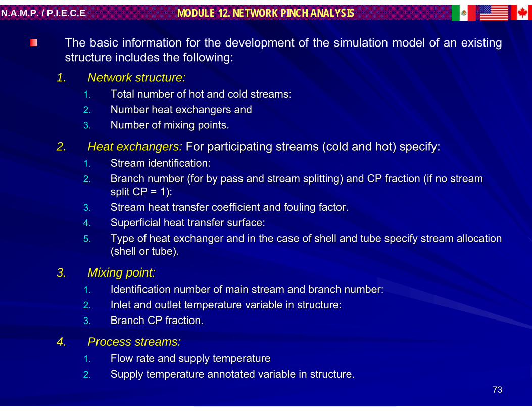
The basic information for the development of the simulation model of an existing structure includes the following:
1.1. Network structure:Network structure:1.1. Total number of hot and cold streams:Total number of hot and cold streams:2.2. Number heat exchangers andNumber heat exchangers and3.3. Number of mixing points.Number of mixing points.
2.2. Heat exchangers:Heat exchangers: For participating streams (cold and hot) specify:For participating streams (cold and hot) specify:1.1. Stream identification:Stream identification:2.2. Branch number (for by pass and stream splitting) and CP fractionBranch number (for by pass and stream splitting) and CP fraction (if no stream (if no stream
split CP = 1):split CP = 1):3.3. Stream heat transfer coefficient and fouling factor.Stream heat transfer coefficient and fouling factor.4.4. Superficial heat transfer surface:Superficial heat transfer surface:5.5. Type of heat exchanger and in the case of shell and tube specifyType of heat exchanger and in the case of shell and tube specify stream allocation stream allocation
(shell or tube).(shell or tube).
3.3. Mixing point:Mixing point:1.1. Identification number of main stream and branch number:Identification number of main stream and branch number:2.2. Inlet and outlet temperature variable in structure:Inlet and outlet temperature variable in structure:3.3. Branch CP fraction.Branch CP fraction.
4.4. Process streams:Process streams:1.1. Flow rate and supply temperatureFlow rate and supply temperature2.2. Supply temperature annotated variable in structure.Supply temperature annotated variable in structure.

7474
MODULE 12. NETWORK PINCH ANALYSISN.A.M.P. / P.I.E.C.E.
The simulation of the network for base case conditions and after corrective actions have been implemented facilitates the specification of the bypass fractions that will be required to operate under normal conditions.
The network simulation model can also be used to assess the performance of increased area or reduced overall heat transfer coefficient in every heat exchanger.
T
UpperBound
LowerBound
Cold stream
Hot stream
Increased Area
Hot stream
Cold stream
Reduced U
AU
t

7575
MODULE 12. NETWORK PINCH ANALYSISN.A.M.P. / P.I.E.C.E.
When various solutions to a problem are possible, the designer must choose the option that minimizes the number of exchanger modifications and minimizes the amount of additional area.
Using steady state simulation, a trial and error procedure must be established particularly in cases where modification of more than one exchanger permits the restoration of target temperatures.
The network must remain operable if operating conditions return to normal. In this case, the network is simulated with increased heat transfer areas and original flow rates and temperatures.

7676
MODULE 12. NETWORK PINCH ANALYSISN.A.M.P. / P.I.E.C.E.
Define Network Structure
Produce equationsthat describe ε and heat balance
about heat exchangers and mixing points
Solve the resultingset of equations
Determine the network responseunder modified conditions
Network under modified conditions
Do TargetTemperatures Fall within the
acceptable bounds?
Network continuesworking
Corrective actionsmust be taken
Yes No
Fig. 2.7 Procedure for assessing of network response under modified conditions.
7777
MODULE 12. NETWORK PINCH ANALYSISN.A.M.P. / P.I.E.C.E.
TIER I: FundamentalsTIER I: Fundamentals
1.1. HEAT RECOVERY NETWORKS (HEN).HEAT RECOVERY NETWORKS (HEN).2.2. STEADY STATE SIMULATION of STEADY STATE SIMULATION of HENsHENs..3.3. OPERABILITY ANALYSIS of OPERABILITY ANALYSIS of HENsHENs..4.4. RETROFIT of RETROFIT of HENsHENs..5.5. MASS EXCHANGE NETWORKS (MEN).MASS EXCHANGE NETWORKS (MEN).6.6. OPERABILITY ANALYSIS of OPERABILITY ANALYSIS of MENsMENs..

7878
MODULE 12. NETWORK PINCH ANALYSISN.A.M.P. / P.I.E.C.E.
3.3. OPERABILITY ANALYSIS of OPERABILITY ANALYSIS of HENsHENs..
3.13.1 Operable Operable HENsHENs (Variations in Operating (Variations in Operating Conditions)Conditions)
3.2 Design for Operability.3.2 Design for Operability.

7979
MODULE 12. NETWORK PINCH ANALYSISN.A.M.P. / P.I.E.C.E.
3.1 OPERABLE 3.1 OPERABLE HENsHENs(Variations in Operating Conditions)(Variations in Operating Conditions)
Variation in Operating Conditions.Variation in Operating Conditions.
Corrective Actions.Corrective Actions.
Corrective Equations for a Single Heat Exchanger Corrective Equations for a Single Heat Exchanger where the Flow and inlet temperatures of one of the where the Flow and inlet temperatures of one of the streams change.streams change.
Simple and Complex Networks. Simple and Complex Networks.

8080
MODULE 12. NETWORK PINCH ANALYSISN.A.M.P. / P.I.E.C.E.
VARIATION IN OPERATING CONDITIONS
Full process design is generally undertaken for a point condition.
For instance, the basis for the design of a chemical plant may be a throughput for 100 tonnes/hour with a feedstock of specific composition being supplied at a specific temperature.
In reality, the plant will rarely operate at this point condition:
Production demands may require a throughput of 110 tonnes/hour some weeks and 80 tonnes/hour other weeks.
Process supply temperatures can show seasonal variations.
Feedstoks compositions can vary.
In addition to changes in process conditions, equipment performance can vary with time, examples:
Catalyst activity.Heat exchanger fouling.
Given these variations, there is a need for chemical plants to be “flexible”. They must be capable of operating efficiently under a variety of conditions.

8181
MODULE 12. NETWORK PINCH ANALYSISN.A.M.P. / P.I.E.C.E.
CORRECTIVE ACTIONS
As mentioned early (sub-section 2.1 Introduction) disturbances propagate through heat exchanger networks by travelling downstream and through heat exchangers. These pathways are clearly shown on the ‘heat exchanger grid diagram’.
The recognition that disturbances can only be propagated ‘downstream’ has important implications for network design. If a particular stream is known to be subject to large disturbances and another stream is known to be particularly sensitive, the engineer would be advised to devise a network structure that does not have a downstream path between the two points.
In many cases the designer will have to introduce process control. This can take the form of:
Increased utility.Using a Bypass to divert some flow around rather than through an
exchanger.
8282
MODULE 12. NETWORK PINCH ANALYSISN.A.M.P. / P.I.E.C.E.
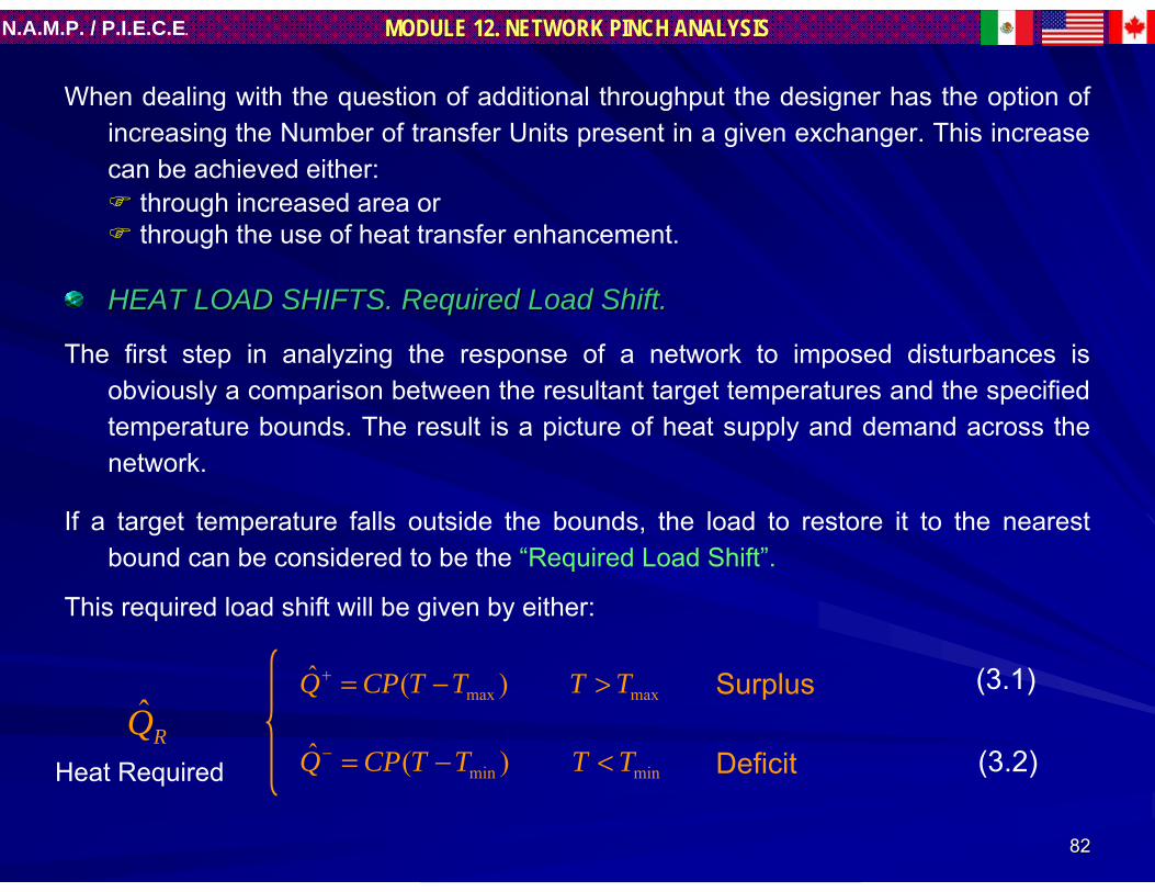
When dealing with the question of additional throughput the designer has the option of increasing the Number of transfer Units present in a given exchanger. This increase can be achieved either:
through increased area orthrough the use of heat transfer enhancement.
HEAT LOAD SHIFTS. Required Load Shift.HEAT LOAD SHIFTS. Required Load Shift.
The first step in analyzing the response of a network to imposed disturbances is obviously a comparison between the resultant target temperatures and the specified temperature bounds. The result is a picture of heat supply and demand across the network.
If a target temperature falls outside the bounds, the load to restore it to the nearest bound can be considered to be the “Required Load Shift”.
This required load shift will be given by either:
minmin )(ˆ TTTTCPQ <−=−
maxmax )(ˆ TTTTCPQ >−=+
RQ̂Heat Required
Surplus
Deficit
(3.1)
(3.2)
8383
MODULE 12. NETWORK PINCH ANALYSISN.A.M.P. / P.I.E.C.E.
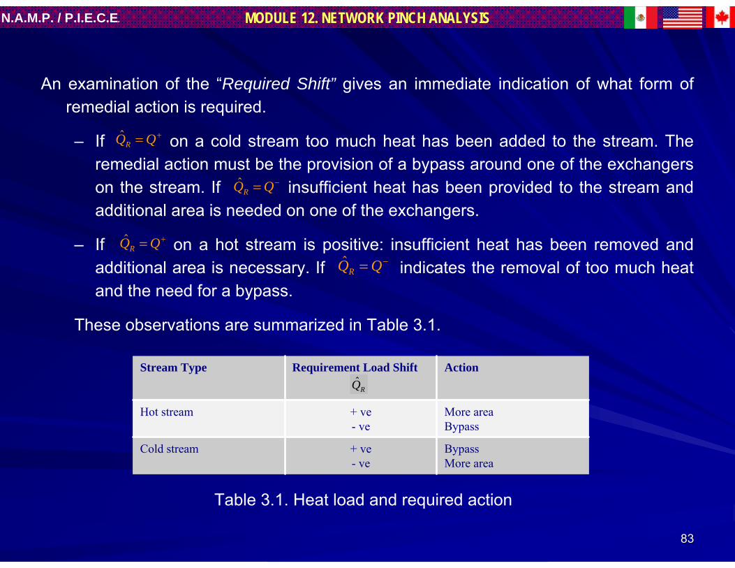
An examination of the “Required Shift” gives an immediate indication of what form of remedial action is required.
– If on a cold stream too much heat has been added to the stream. The remedial action must be the provision of a bypass around one of the exchangers on the stream. If insufficient heat has been provided to the stream and additional area is needed on one of the exchangers.
– If on a hot stream is positive: insufficient heat has been removed and additional area is necessary. If indicates the removal of too much heat and the need for a bypass.
These observations are summarized in Table 3.1.
+= QQRˆ
−= QQRˆ
+= QQRˆ
−= QQRˆ
BypassMore area
+ ve- ve
Cold stream
More areaBypass
+ ve- ve
Hot stream
ActionRequirement Load ShiftStream Type
Table 3.1. Heat load and required action
RQ̂

8484
MODULE 12. NETWORK PINCH ANALYSISN.A.M.P. / P.I.E.C.E.
HEAT LOAD SHIFTS. Available Shift.HEAT LOAD SHIFTS. Available Shift.
If a target temperature is well within its required bounds, it has a “required shift” of zero. However, with such a stream there may still be scope for shifting heat down the paths by going to one of the bounds. Such heat load shifts can also generally be undertaken in either direction.
The “Available shifts” are given by:
Finally, it is recognized that a stream having a “required heat shift” also have an ‘available shift’. This shift is in the same direction as the ‘required shift’ and is the load that is necessary to take the stream to the furthest bound.
)(ˆminTTCPQ −=+
)(ˆmaxTTCPQ −=−
(3.3)
(3.4)

8585
MODULE 12. NETWORK PINCH ANALYSISN.A.M.P. / P.I.E.C.E.
Summarizing LOAD HIFTS.Summarizing LOAD HIFTS.
Now, in summary, all streams provide two potential shifts:– A stream that falls within its bounds does not have a ‘required shift’ but
provides ‘available shifts’ in two directions.– A stream that falls outside its bounds has a ‘required shift’ and an ‘available
shift’. This available shift is in the same direction as the ‘required shift’. They are of different magnitude.
Comparison of ‘required’ and ‘available’ shifts allow us to observe:1. The stream matches that can be used to satisfy flexibility needs:2. The maximum load shifts that can be employed with a given match:3. A guide to structural changes that can be made in order to achieve flexibility
through heat recovery rather than through the use of additional utility.

8686
MODULE 12. NETWORK PINCH ANALYSISN.A.M.P. / P.I.E.C.E.
By a way of illustration consider the results presented in Table 3.2.Following a disturbance to the operating condition, it is found that streams H1 and C1
are no longer within bounds. Each requires the shifting of 20 units of heat to restore proper operation.
Examination of the Table shows that the deficit on C1 cold be supplied using any of the hot streams. The surplus on H1 could be utilized on either C1 or C2.
- 10+ 10--C3- 15+ 51--H3
- 20+ 30--C2- 10+ 40--H2
- 45--- 20C1--+ 40+20H1
Q-Q+QRQ-Q+QR
AvailableRequiredStream
AvailableRequiredStream
Cold streamHot stream
Table 3.2 Heat demand and availability of streams after disturbed conditions. Action required for the restoration of target temperatures.
The final choices will be based on existing paths and required additional area. As a last resort a new path (i.e. new match) could be generated.
LOAD HIFTS. EXAMPLELOAD HIFTS. EXAMPLE

8787
MODULE 12. NETWORK PINCH ANALYSISN.A.M.P. / P.I.E.C.E.
CORRECTIVE EQUATIONS FOR A SINGLE HEATCORRECTIVE EQUATIONS FOR A SINGLE HEATEXCHANGER WHERE THE FLOW AND INLETEXCHANGER WHERE THE FLOW AND INLETTEMPERATURES OF ONE OF THE STREAM CHANGES.TEMPERATURES OF ONE OF THE STREAM CHANGES.
An examination of required and available heat shifts provides a guide as to which streams can be used to provide flexibility and it indicates the form of action to take. However, the concept makes no consideration of temperatures field or of exchanger technology.
A shift identified in this manner may prove infeasible or extremely expensive.
In this section a single exchanger will be considered where the flow rate and inlet temperature of one of the streams changes.
An appropriate modification must be made to the unit in order to restore both outlet temperatures to their original values.
Equations relating change in exchanger outlet temperature with changes in exchanger effectiveness can be derived for each type of modification.

8888
MODULE 12. NETWORK PINCH ANALYSISN.A.M.P. / P.I.E.C.E.
ADDITION OF HEAT TRANSFER AREA.ADDITION OF HEAT TRANSFER AREA.
Effectiveness Needs.Effectiveness Needs.Referring to Figure 3.1.1, the addition of heat
transfer area to an exchanger will result in the hot outlet temperature (T) moving to lower values and the cold outlet temperature (t) moving to higher values.
Consider the case in which following a disturbance the outlet temperature of the hot stream is T2
(N) and needs to be brought to a value T2
(O).
The question that arises here is, how much area must be added to the unit to achieve this objective?
T1T2
t2t1
T : CP min streamt : CP max stream
T
H
Fig. 3.1 Single heat exchanger
T2
T1
t1
t2

8989
MODULE 12. NETWORK PINCH ANALYSISN.A.M.P. / P.I.E.C.E.
Expressions for the exchanger outlet temperatures can be written from the definition of thermal effectiveness.
For the existing condition:
For the desired condition:
Combining equations (3.5) and (3.7) the following expression can be derived
Which after rearranging gives
This expression gives the change in exchanger effectiveness (ε) required to bring about the desired corrective changed on T2.
Δ−= )(1
)(2
OO TT ε Δ+= )(1
)(2
OO Ctt ε(3.5) (3.6)and
Δ−= )(1
)(2
NN TT ε
Δ−−=−= )(ˆ )()()(2
)(22
ONON TTT εε
(3.7)
(3.8)
Δ−=−= 2)()(
ˆˆ TON εεε (3.9)

9090
MODULE 12. NETWORK PINCH ANALYSISN.A.M.P. / P.I.E.C.E.
The same exercise can be carried out for the case where the change takes place in t2(O)
In such case, the new effectiveness becomes
In the above example the hot stream had the lower heat capacity flow rate. Similar equations to (3.9) and (3.10) can be derived for the case where the cold stream has the lower value. These results are:
Table 3.3 summarizes these results.
Δ=−=
CtONC 2)()( ˆ
ˆ εεε (3.10)
Δ−=−=
CTON 2)()(ˆ
ˆ εεεΔ
−=−=CtON 2)()( ˆ
ˆ εεε(3.11) (3.12)and
Cold stream
Hot stream
Outlet temperature of CPmax stream
Outlet temperature of CPmin stream
CPmin
Δ−= T̂ε̂
Δ= t̂ε̂
Δ−=
CT̂ε̂
Δ=
Ct̂ε̂
Table 3.3 Corrective equations. Effectiveness needs of an exchangerFor a required temperature shift of either outlet temperature.

9191
MODULE 12. NETWORK PINCH ANALYSISN.A.M.P. / P.I.E.C.E.
Area needs.Area needs.Changes in effectiveness can be converted into changes in area once the type of
exchanger is known.For instance, for a pure counter-current arrangement, thermal effectiveness and
Number of transfer Units are related according to
For this expression:
Now, letting NTU(O) and NTU(N) be the initial and the new exchanger Number of Transfer Units respectively, then the NTU change is given by
This equation gives the required NTU increase the exchanger must undergo in order to meet the specified target temperature. The additional area can be calculated from
)1(
)1(
11
CNTU
CNTU
Cee
−−
−−
−−=ε
)1(1
1ln
CC
C
NTU−
⎟⎠⎞
⎜⎝⎛
−−
=
ε
(3.13)
(3.14)
( )( )( )( )
)1(1111ln
ˆ)()(
)()(
CCC
UTNNO
ON
−
⎥⎦
⎤⎢⎣
⎡−−−−
=εεεε
minˆˆ CPUTNAU ⋅=
(3.15)
(3.16)
9292
MODULE 12. NETWORK PINCH ANALYSISN.A.M.P. / P.I.E.C.E.
Mass Flow Rate manipulation
Since the effectiveness of an exchanger is a function of the CP-ratio, a change to the mass flow rate of either of the streams about a single exchanger will result in a change to the thermal effectiveness of the unit. Bypass can therefore be used to achieve a desired temperature correction.
Consider manipulation of the stream exhibiting the lowest CP. The fraction of the flow of the manipulated stream actually passing through the exchanger will be represented by f.
For a bypass to be applicable the exchanger must be larger than it is actually needed for one of the operating cases. Assume that this is the base case and under this situation the bypass operates partially open and f(O) is the fraction of the flow passing through the exchanger.
ADDITION OF HEAT TRANSFER AREAADDITION OF HEAT TRANSFER AREA..

9393
MODULE 12. NETWORK PINCH ANALYSISN.A.M.P. / P.I.E.C.E.
If temperature T2 in Figure 3.1.2 needs to be reduced the bypass valve must close. Conversely, when T2 is to be increased the bypass valve opens. Assume the new flow fraction through the exchanger becomes f(N).
Denoting T2’(O) as the initial condition of T2
’, the following expression can be written:
T2’(O) = T1 - Δε(O)
A heat balance about mixing point gives
T2(O) = (1 – f(O))T1 + f(O)T2
’(O)
Combining the two equations yields
T2(O) = T1 – f(O) Δε(O)
When bypass valve operates T2’(O) becomes T2
’(N)
and is given by
T2’(N) = T1 - Δε(N)
Again, a heat balance about the mixing point gives
T2(N) = (1 – f(N))T1 + f(N)T2
’(N)
Combination of equations (3.1.20) and (3.1.21) gives
T2(N) = T1 – f(N) Δε(N)
f
1 - f
T2 T1
T2’
t1 t2
T : hot streamt : cold stream
Fig. 3.2 Heat exchanger fitted with bypass.
(3.18)
(3.17)
(3.19)
(3. 20)
(3. 21)
(3. 22)

9494
MODULE 12. NETWORK PINCH ANALYSISN.A.M.P. / P.I.E.C.E.
The total change in outlet temperature T2 can be obtained by combining equations (3.19) and (3.22):
A similar analysis performed for temperature t2 gives
In the case where the bypass valve operates between an initial condition of fully closed and a final condition of partially open, then f(O) = 1 and f(N) = f. Equation (3.23.) reduces to
Similarly it can be shown that
Equations (3.25) and (3.26) relate the required temperature change to f and new exchanger effectiveness (ε(N)).
For a given or , f can be calculated iteratively.The exchanger effectiveness following a flow change can be calculated using the
procedures given in sub-section “updating exchanger effectiveness and NTU” of “2.2 Response Equations” .
2̂T2̂t
( ))()()()(2̂
OONN ffT εε −Δ−=
( ))()()()(2̂
OONN ffCt εε −Δ−=
(3.23)
(3.24)
( ))()(2̂
ONfT εε −Δ−=
( ))()(2̂
ONfCt εε −Δ−=
(3.25)
(3.26)

9595
MODULE 12. NETWORK PINCH ANALYSISN.A.M.P. / P.I.E.C.E.
Now consider the case where one of the outlet temperatures of the exchanger (say T2) needs to be restored to its original value. For the case where only mass flow rate disturbances exist, it can be demonstrated that the flow fraction through the exchanger can be found from:
Specific equations like this can be derived for any combination of disturbances (temperature and flow rate).
Summarizing:Table 3.4 summarizes the general ‘Corrective Equations’ for flow rate manipulation.
( ) )(conditions case base
)( NO fεε = (3.27)
Cold stream
Hot stream
Outlet temperature of CPmaxstream
Outlet temperature of CPmin stream
CPmin stream
MASS FLOW RATE MANIPULATION
( ))()()(ˆ ONO fT εε −Δ−=
( ))()()()(ˆ ONOO fCT εε −Δ−=
( ))()()()(ˆ ONOO fCt εε −Δ=
( ))()()(ˆ ONO ft εε −Δ=
Table 3.4. Corrective Equations. Mass flow rate manipulation for the correctionof outlet temperatures. Initial condition of valve: shut.

9696
MODULE 12. NETWORK PINCH ANALYSISN.A.M.P. / P.I.E.C.E.
3.3. Operability Analysis of Operability Analysis of HENsHENs..
3.1 Operable 3.1 Operable HENsHENs (Variations in (Variations in Operating Conditions)Operating Conditions)
3.2 Design for Operability.3.2 Design for Operability.

9797
MODULE 12. NETWORK PINCH ANALYSISN.A.M.P. / P.I.E.C.E.
3.2 DESIGN FOR OPERABILITY3.2 DESIGN FOR OPERABILITY
NETWORK INTERACTIONSNETWORK INTERACTIONS
So far only modifications to single heat exchangers have been considered. Attention must be paid to the influence of network interactions on the necessary modifications..
Network structure influences the design process in two ways:Network structure influences the design process in two ways:
First, it affects the order in which modifications must be consiFirst, it affects the order in which modifications must be considered.dered.
Second, the network response is as important as any individual eSecond, the network response is as important as any individual exchanger xchanger responseresponse..

9898
MODULE 12. NETWORK PINCH ANALYSISN.A.M.P. / P.I.E.C.E.
ORDER OF UNDERTAKING NETWORK MODIFICATIONS.ORDER OF UNDERTAKING NETWORK MODIFICATIONS.
Consider the network problem shown in Figure 3.3 Assume temperatures T5 and T7have been disturbed and need to be restored. Control of temperature T7 can be achieved by means of a bypass placed about exchanger E1. Temperature T5 can be restored through the provision of additional area on exchanger E2.
Assume that the designer decides to look at the restoration of T5 first. The amount of area that needs to be added is computed on the basis of temperatures T2, T4 and T5.
Now the designer tackles the bypass about exchanger E1. However, the result of this exercise is a change in temperature T2. The basis of the initial modification (toE1) is now prejudiced. The designer now has to redo this modification
C
C
T2 T1T3
T4 T5
T6 T7
δ
CPh = CPmin
E1E2
Fig. 3.3 Network responses and damping.
Clearly the order in which modification are considered is important. It is also clear thatupstream changes must be considered first.

9999
MODULE 12. NETWORK PINCH ANALYSISN.A.M.P. / P.I.E.C.E.
NETWORK RESPONSES.NETWORK RESPONSES.
Consider Figure 3.4 This shows a case in which a target temperature Tx needs to be increased by an amount (δ). Assume that any of the three exchangers on the stream could be used to achieve this objective.
C
E1
E2
E3
δ3 δ2 δ1 Tx
CPmin = CPh
Fig. 3.4 Network response and dumping.
Exchanger E1 is closet to the ‘target point’. The modification necessary to this exchanger can be calculated directly from the equations derived before for single exchangers.
Exchanger E2 is separated from the ‘target point’ by exchanger E1. The question that now must be asked is ‘how large is the correction that must be made to the outlet temperature of this exchanger in order to provide the required change to the target temperature?’

100100
MODULE 12. NETWORK PINCH ANALYSISN.A.M.P. / P.I.E.C.E.
A change to this outlet temperature constitutes a disturbance to the temperature of exchanger E1. The response of E1 to this change is dependent on its effectiveness and CP ratio. In this case it can be shown that:
The important observation here, as known by experienced industrial engineers, is the presence of another exchanger between one being considered for modification and the target point dampens the effect of the proposed modification.
The damping can be determined from the steady state response developed in the sub-section “Single and complex networks. Response equations” of section 3.1 Operable Network.
Starting at the exchanger furthest ‘upstream’ (E3), given that the hot stream has the lower heat capacity flow rate, the response of the cold stream outlet temperature to an increase in the effectiveness of the exchanger is (from Table 3.3)
)1( )(1121
OC εδδ −=
3333 ε̂δ Δ= C
(3.28)
(3.29)

101101
MODULE 12. NETWORK PINCH ANALYSISN.A.M.P. / P.I.E.C.E.
The damping introduced by exchanger E2 is (from table XX):
and that from exchanger E1 is:
So, the final effect on the ‘target point’ temperature is:
where superscript 3 indicates the effect after E3.
Now, consider exchanger E2. Also assume that a modification has been made to exchanger E3. The result of the modification to exchanger E3 is a change in the temperature lift (Δ) of exchanger E2. Taking this into account, the cold stream outlet temperature change resulting from a change in the effectiveness of exchanger E2 is:
The damping associated with the presence of exchanger E1 is:
So, the final effect on the ‘target point’ temperature is:
)1( )(2232OC εδδ −= (3.30)
(3.31)
(3.32)
(3.33)
(3.34)
(3.35)
)1( )(1121
OC εδδ −=
)1)(1(ˆ )(11
)(21333
31
OO CCC εεεδ −−Δ=
23222 ˆ)( εεδ −Δ= C
)1( )(112
21
OC εδδ −=
)1(ˆ)( )(112322
21
OCC εεδδ −−Δ=

102102
MODULE 12. NETWORK PINCH ANALYSISN.A.M.P. / P.I.E.C.E.
Finally, consider a modification to exchanger E1. The response of this exchanger to changed effectiveness occurs directly at the ‘target point’ and is:
Knowing the structure of the ‘path’ a general equation relating the individual response with the required overall response can be written:
The result is a set of equations (3.2.10, 3.2.9, 3.2.3 and 3.2.2) that can be solved in order to evaluate the different combination of modifications that will provide the required result.
121111 ˆ)( εδδ −Δ= C (3.36)
11
)(112
)(11
)(2231 )1()1)(1( δεδεεδδ +−+−−= OOOT CCC (3.37)

103103
MODULE 12. NETWORK PINCH ANALYSISN.A.M.P. / P.I.E.C.E.
COST EFFECTIVE NETWORK MODIFICATIONCOST EFFECTIVE NETWORK MODIFICATION
The cost effective modification to a network is not necessarily the one that uses the last additional area.
It is generally the one having the minimum of changes. If the required modification can be achieved using heat transfer enhancement rather than additional area this is the direction to go for it avoids the installation of a new exchanger with its associated piping, civil and instrumentation costs.
There is a hierarchy of options:
1 Use a Heat Transfer Enhancement on just one Exchanger.
2 Use of Heat Transfer Enhancement in general.
3 Installation of just one new exchanger in existing structure.
4 Installation of one new exchanger in existing structure and the use of enhancement on others.
5 Installation of more than one exchanger in existing structure.
6 New heat recovery match unless justified by energy saving rather than flexibility requirement.

104104
MODULE 12. NETWORK PINCH ANALYSISN.A.M.P. / P.I.E.C.E.
The scope for using heat transfer enhancement on any duty can easily be determined;
First, the exchanger is examined to determine the extent to which the overall heat transfer coefficient can be improved. This is then converted to a change in Number of Heat Transfer Units. Finally, the resultant change in effectiveness is obtained.
In some cases the use of heat transfer enhancement may be ruled by severe pressure drop constraints.
However, it is often possible to overcome such constraints through making judicious changes to exchanger header arrangements.

105105
MODULE 12. NETWORK PINCH ANALYSISN.A.M.P. / P.I.E.C.E.
DISTRIBUTION OF AREA BETWEEN EXCHANGERSDISTRIBUTION OF AREA BETWEEN EXCHANGERS
In some occasions it will be found that more than one exchanger will have to be modified in order to achieve a single flexibility objective. Under these circumstances the designer is interested in determining a cost effective distribution of area between the exchangers.
Again consider the network shown in Figure 3.2.2. Assume that it has been identified that in order to achieve the flexibility objective area must be added to exchangers E1 and E2. The distribution of this area now has to be determined.
For the manipulation of two exchangers equation (3.2.10.) becomes:
where
and
The two unknowns are and .The optimum distribution could be found through exhaustive search. Each term varies
between zero and the limit given by equation (3.2.3.). For each value of the value of necessary to achieve the objective can be calculated. Then, from these two values the individual and overall increased in Number of Transfer Units can be found.
1)(
112 )1( δεδδ +−= OT C
2222 ε̂δ Δ= C
12111 ˆ)( εδδ −Δ= C
1̂ε 2ε̂
1̂ε2ε̂
(3.38)
(3.39)
(3.40)

106106
MODULE 12. NETWORK PINCH ANALYSISN.A.M.P. / P.I.E.C.E.
The results of such exercises are shown in Figure 3.5 for values of individual effectiveness ranging from 0.4 to 0.9.
It is seen that the thermal effectiveness of the exchangers plays an important role in determining the cost effective area distribution.
Two regions can be observed:
Region 1.
A region in which the addition of area to exchanger 1 should be maximized. This is seen to be not only the case where E1 has the lower effectiveness but also where the adverse effects of a higher effectiveness on exchanger 1 are counteracted by its damping effect.
Region 2.
A region in which the effectiveness of E1 is much higher than that of E2 and despite the damping associated with the unit the best policy is the addition of area to E2.

107107
MODULE 12. NETWORK PINCH ANALYSISN.A.M.P. / P.I.E.C.E.
Figure 3.5 Required NTU v. ε for counter-current exchangers

108108
MODULE 12. NETWORK PINCH ANALYSISN.A.M.P. / P.I.E.C.E.
SIMPLE AND COMPLEX NETWORKSSIMPLE AND COMPLEX NETWORKS..
Heat exchanger networks may exhibit simple or complex structures, The latter is characterized by the presence of feedback loops in the network.
What is a FEEDBACK LOOP in a HEN?Consider the HEN shown in Figure 3.6 and follow the path of a disturbance on stream 1
around the network.
E1E2
E31
2
3
Path of disturbance
Feedback Loop
Fig. 3.6 The presence of a feedback in the network make it a Complex network.
109109
MODULE 12. NETWORK PINCH ANALYSISN.A.M.P. / P.I.E.C.E.
Following the path of a disturbance on stream 1 around the network we can see that first affects the outlet temperature of exchanger 1. This form the inlet to exchanger 2 and has an effect on the cold stream leaving exchanger 2 (stream 3). This disturbance is dampened as the stream passes through exchanger 3 but some level of disturbance is still present when this stream now enters exchanger 1. Exchanger 1 which was the first unit to encounter the disturbance now encounters the downstream effects of the disturbance.
SIMPLE AND COMPLEX NETWORKS
Structures which contain cyclic elements (I.e. elements that are repeated) or overlapping loops are classified as being COMPLEX NETWORKS. In contrast with the structure shown in Figure 3.2.5 a network structure containing a loop but it does not provide feedback is classified as having a ‘SIMPLE’ STRUTURE. The Figure 3.7 shows a simple structure.
E1

110110
MODULE 12. NETWORK PINCH ANALYSISN.A.M.P. / P.I.E.C.E.
1
2
3
4
E4
E2E1
E3
Figure 3.7 Simple structure: loop without feedback.
The procedure for determining the response where feedback loops exist involves the derivation of a feedback factor which is a function of the network structure. This factor includes all the dampening elements that a disturbance encounters as it propagates around a loop.
Most industrial heat recovery networks are of the simple variety for they use close to the minimum number of units and only rarely contain cyclic elements or complex multiple loops.

111111
MODULE 12. NETWORK PINCH ANALYSISN.A.M.P. / P.I.E.C.E.
MULTIPLE OBJECTIVESMULTIPLE OBJECTIVES
It is often the case that operating changes result in the need to restore more than one target temperature. It may then be found that an exchanger chosen to manipulate one target also has a downstream path to another target.
The complexity of the problem can be further increased if the remedial action proposed for one objective actually has a detrimental effect upon another objective.
Consider Figure 3.8 which shows only part of a network. Following operating disturbances it is necessary to decrease T2 by and T10 is required to increase by .)(1̂0 CT
)(2̂ CT
C
C
E1
E2
E3
T1T2
T3T4
T5T6
T7 T8 T9 T10
CPmin = CPc
CPmin = CPc
CPmin = CPh
Fig. 3.8 Multiple objectives.

112112
MODULE 12. NETWORK PINCH ANALYSISN.A.M.P. / P.I.E.C.E.
It is seen that T2 can only be restored by increasing the area of exchanger E1. However, it is also seen that any change to E1 also affects T10. This temperature can also be manipulated by changes to exchanger E3.
The problem is solved by setting up and solving the following system of simultaneous equations:
where:
Equations (3.41) and (3.42) represent the effect of the modification of exchangers E3 and E1 upon target temperatures T10 and T2 respectively.
Their solution together with expressions (3.43) to (3.44) yield the necessary effectiveness changes to exchangers E3 and E1.
101)(
1223ˆ)1)(1( TC O =+−− δεεδ
2*1
)(223
ˆ)1( TC O =+− δεεδ
(3.41)
(3.42)
3333 ˆ Δ= Cεδ
( )[ ]223111 1ˆ εδεδ C−−Δ=
( )[ ]223111*1 1ˆ εδεδ CC −−Δ−=
(3.43)
(3.44)
(3.45)

113113
MODULE 12. NETWORK PINCH ANALYSISN.A.M.P. / P.I.E.C.E.
TIER I: FUNDAMENTALSTIER I: FUNDAMENTALS
11 HEAT RECOVERY NETWORKS (HEAT RECOVERY NETWORKS (HENsHENs).).
22 STEADY STATE SIMULATION of STEADY STATE SIMULATION of HENsHENs..
33 OPERABILITY ANALYSIS of OPERABILITY ANALYSIS of HENsHENs..
44 RETROFIT of RETROFIT of HENsHENs..
55 MASS EXCHANGE NETWORKS (MASS EXCHANGE NETWORKS (MENsMENs).).
66 OPERABILITY ANALYSIS of OPERABILITY ANALYSIS of MENsMENs..

114114
MODULE 12. NETWORK PINCH ANALYSISN.A.M.P. / P.I.E.C.E.
4 RETROFIT OF 4 RETROFIT OF HENsHENs..
4.1 4.1 Introduction.Introduction.
4.2 Retrofit Targeting.4.2 Retrofit Targeting.

115115
MODULE 12. NETWORK PINCH ANALYSISN.A.M.P. / P.I.E.C.E.
INTRODUCTION.INTRODUCTION.
A vital lesson from pinch technology has been the need to set targets. The principles is to predict what should be achieved (targeting), and to then set out to achieve it (design).
Applications of process integration fall into two categories -grassroots design and retrofit. In retrofit is applied the same thermodynamic principles that underlie established pinch technology and the philosophy of targeting prior to design is maintained.
In the context of retrofitting, this implies the setting of targets for:- Energy saving- Capital cost- Payback.
The targets recognize the specifics of the existing design.

116116
MODULE 12. NETWORK PINCH ANALYSISN.A.M.P. / P.I.E.C.E.
HOW ARE RETROFIT PROJECTS TACKLED?HOW ARE RETROFIT PROJECTS TACKLED?
Retrofit projects are tackled in three current approaches :
1. Inspection. Examine the plant and select a project intuitively. This approach are called “cherry picking”. The result is never quite certain. There is usually a doubt remaining - “Could there be a better answer?”
2. Computer search. Those who have process-synthesis computer programs may ask “Why not generate many alternative new designs? Hopefully, one of these may be similar to the existing plant and will thus spark off a reasonable retrofit project.” This approach can consume a lot of computation time and be very expensive. More important, it does not provide any insight into the problem and does not necessarily generate a good solution.
3. Pinch technology. Apply pinch principles and incorporate process insight during the design. Although this approach has been used industrially with some success, it is, strictly speaking, an improvisation on methodology aimed at grassroots design. User experience is crucial for a good result.

117117
MODULE 12. NETWORK PINCH ANALYSISN.A.M.P. / P.I.E.C.E.
RETROFIT BY INSPECTIONRETROFIT BY INSPECTION
Fig. 4.1 shows a simple heat-exchanger network in the grid representation. Let us consider an energy retrofit for this network.
Initial inspection would suggest contacting streams 1 and 5 at the cold end of the process. This would reduce the heat loads on cooler C1 and on the heater. Stream 1 is chosen in preference to stream2 because of its significantly higher heat-capacity flowrate.
However, the integration of a new heat exchanger is not completely straightforward. The new exchanger would affect the temperature in “downstream” exchangers 1 and 4 which would lead to the need for additional area here. Then if additional area were needed in exchanger 4 anyway, we should once more consider stream 2, with a view to reducing the load on cooler C2.
With this type of reasoning, a network may result as shown in Fig.2. The overall saving in energy is 2,335 kW.
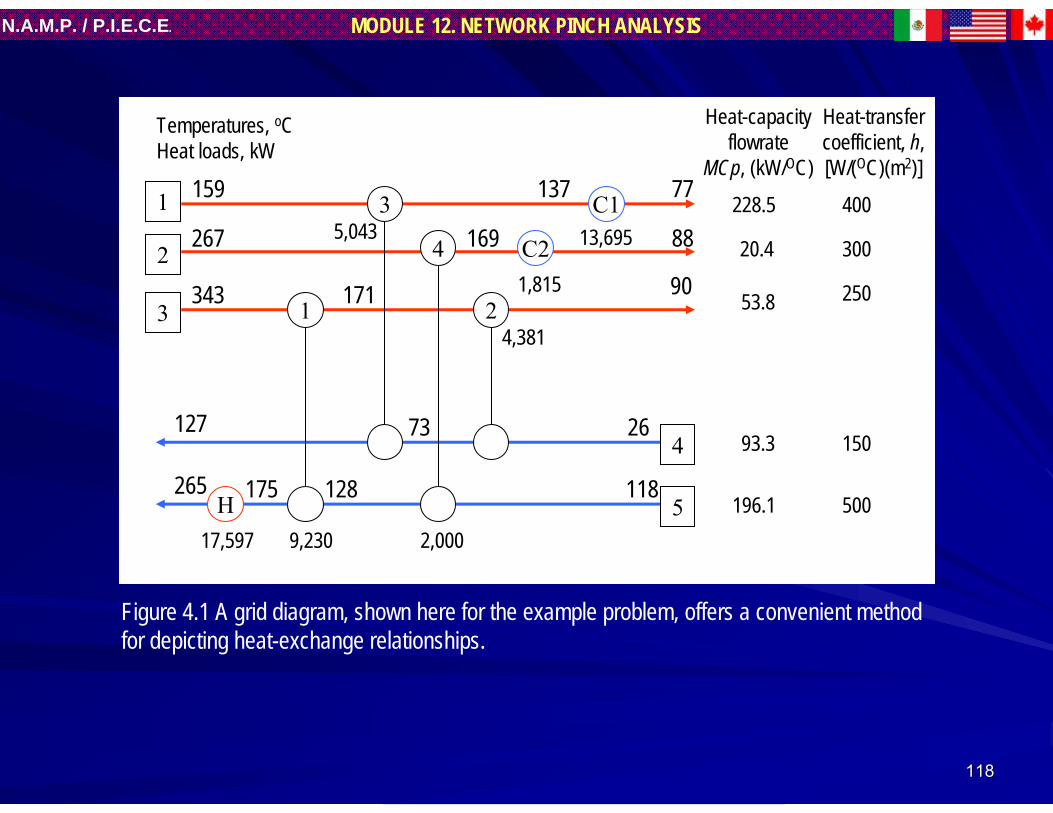
118118
MODULE 12. NETWORK PINCH ANALYSISN.A.M.P. / P.I.E.C.E.
1
2
3
4
5
1
3
4
2
C2
C1
H
Temperatures, oCHeat loads, kW
159 137 77
267 169 88
343 171 90
2673127
118128175265
9,23017,597
5,043
2,000
4,381
1,815
13,695228.5
20.4
53.8
93.3
196.1
400
300
250
150
500
Heat-capacityflowrate
MCp, (kW/OC)
Heat-transfercoefficient, h,[W/(OC)(m2)]
Figure 4.1 A grid diagram, shown here for the example problem, offers a convenient method for depicting heat-exchange relationships.

119119
MODULE 12. NETWORK PINCH ANALYSISN.A.M.P. / P.I.E.C.E.
1
2
3
4
5
3
2
C1
H
Temperatures, oCHeat loads, kW
159 137 77
267 141 88
343 171 90
2673127
118128187265
9,23015,262
5,042
2,570
4,381
1,815
11,930
11
4 C2
129
140 1271,765
Figure 4.2 Retrofit by inspection prompts the addition of a new exchanger and revised duties.

120120
MODULE 12. NETWORK PINCH ANALYSISN.A.M.P. / P.I.E.C.E.
But why should we choose this level of energy savings? By installing more exchanger area (I.e., investing more capital) we could have saved more energy. By installing less exchanger area, we could save on capital. Although we would save less energy.
An economic analysis for various energy-recovery level is shown in Table 1. A simple calculation shows that the “set point” chosen in Fig. 2 saves significant energy (about 13%) at a good payback (2 years).
But how good is this result? There many be a doubt remaining. Could there be a better solution?
Setpoint Investment,£ million
Savings,£ million/yr
Payback,yr
1 0.184 0.111 1.72 0.293 0.148 2.03 0.484 0.192 2.54 0.670 0.213 3.1
Table 4.1 Project economics of retrofit by inspection: higher savings, longer payback.

121121
MODULE 12. NETWORK PINCH ANALYSISN.A.M.P. / P.I.E.C.E.
4 RETROFIT OF 4 RETROFIT OF HENsHENs..
4.1 4.1 Introduction.Introduction.
4.2 Retrofit Targeting.4.2 Retrofit Targeting.

122122
MODULE 12. NETWORK PINCH ANALYSISN.A.M.P. / P.I.E.C.E.
RETROFIT TARGETINGRETROFIT TARGETING
SETTING RETROFIT TARGETINGSETTING RETROFIT TARGETING
Fig. 4.3 shows an energy/area plot, which relates the energy requirement with the heat-exchange area used in a given process.- Point A represents a case where the composite curves are close (low ΔTmin), with corresponding high energy recovery but high investment in area.- Point C relates to composite curves that are more widely spaced, yielding lower energy recovery but less investment. We have a continuos curve representing networks that are all on target for both energy and area.- Point B represents the optimum tradeoff with the lowest total cost.
The area below the curve is tinted and marked “infeasible”. It is not possible for a design to be better than target..
But where would a retrofit candidate be situated? In most cases, we would expect it to be above the line, say at Point X. A design at Point X does not take best advantage of its installed area or, to put it another way, it does not recover as much energy as it should.
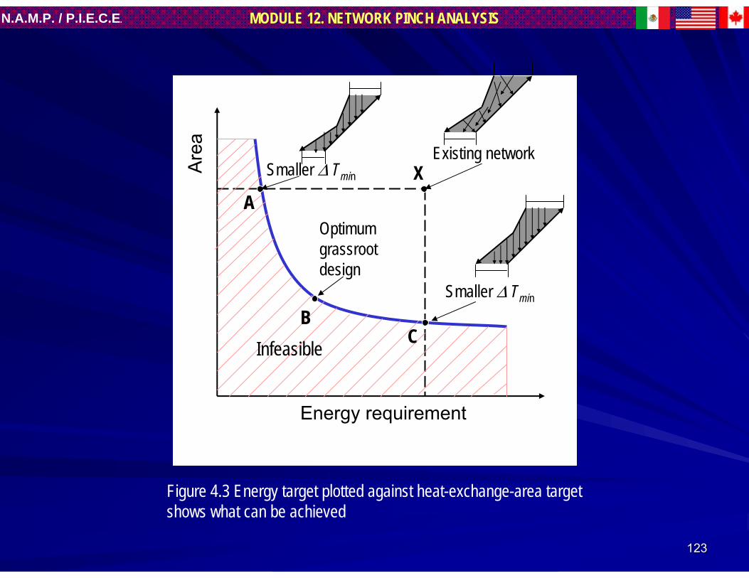
123123
MODULE 12. NETWORK PINCH ANALYSISN.A.M.P. / P.I.E.C.E.
A
CB
XSmaller Δ Tmin
Smaller Δ Tmin
Existing network
Optimumgrassrootdesign
Infeasible
Are
a
Energy requirement
Figure 4.3 Energy target plotted against heat-exchange-area target shows what can be achieved

124124
MODULE 12. NETWORK PINCH ANALYSISN.A.M.P. / P.I.E.C.E.
TARGETING PHILOSOPHY.TARGETING PHILOSOPHY.
It is often assumed that good retrofits should be conducted by aiming toward the optimum new design. We can now see that this does not make sense. Who is prepared to throw away area that has already been paid for, if an optimum new design calls for less area? Our first objective must be to use the existing area more effectively.
In others words, we should try to improve on the ineffective use of area due to criss-crossing, while shifting the composite curves closer to save energy.
The ideal point to aim for from Point X in Fig. 4.3 would therefore be Point A.
here we would save as much energy as possible using the existing area. However, in practice we usually have to invest some capital to make changes to an existing network, thus increasing area. This leads to a “path” similar to that shown in Fig. 4.4

125125
MODULE 12. NETWORK PINCH ANALYSISN.A.M.P. / P.I.E.C.E.
A
B
XSmaller Δ Tmin Existing network
Optimum grassrootdesign
Infeasible
Are
a
Energy requirement
Likely pathof retrofit
Areaalreadyinvested
Not Retrofit shouldnot discard existing area
Figure 4.4 A retrofit should try to reach Point A, not B, to take full advantage of the existing area

126126
MODULE 12. NETWORK PINCH ANALYSISN.A.M.P. / P.I.E.C.E.
Usually many options are available to the designer, so many paths will exist, as shown in Fig. 4.5. Clearly, the cost effectiveness of each of these curves will be different. The lower the curve, the lower the investment for a given savings.
Assume that the best cure is that shown in Fig. 4.5. The shape of this curve is typical. Its slope increases with increasing investment. This implies that the payback period increases with investment level.
By using given costs of area and energy, the “best curve” can readily be transformed into a savings/investment relationships, as shown in Fig. 4.6. This curve relates annual energy savings to investment and payback. The project scope is usually set by one of these three criteria:
- Savings- Investment or- Payback period.
For example, in Fig. 4.6, for an investment of a1, we achieve a savings of b1 at a 1-year payback. If we target a 2-years payback period, we can achieve a savings of b2. Now we have genuine retrofit targets!.
Unfortunately, the “best curve” is difficult to determine. It is a function of plant layout andprocess constraints.

127127
MODULE 12. NETWORK PINCH ANALYSISN.A.M.P. / P.I.E.C.E.
Are
a
Energy requirement
Best retrofitExisting design
Fig. 4.5 many paths are possible for retrofit, but bottom curve, whose shape is typical, is the best.

128128
MODULE 12. NETWORK PINCH ANALYSISN.A.M.P. / P.I.E.C.E.
Sav
ings
per
yea
r
Investmenta1 a2
b1
b2
1 year2 years
5 yearsBest retrofit
Payback period
Figure 4.6 Best curve for area/energy can be translated into a savings/investment plot

129129
MODULE 12. NETWORK PINCH ANALYSISN.A.M.P. / P.I.E.C.E.
AREA EFFICIENCYAREA EFFICIENCYA assumption would be that the network, after retrofit, will use at least as effectively as
before; if the project is good, then it is not likely to place new area in a manner that reduces the effectiveness of the area usage overall !!.
An “area efficiency”, α, is equal to the ratio of minimum area required (target) to that actually used for a specific energy recovery:
The value of α can be expected to be less than unity in practical designs. A value of the unity would indicate “no criss-crossing”. The lower the value of α, the poorer the use of area, and the more severe the criss-crossing.
If we assume that α is constant over the full energy span, we would obtain the curve shown in Fig. 4.7. This curve forms a boundary for design.
We can now distinguish four distinct regions in the energy/area plot (Fig. 4.8):- A region in which designs area infeasible (be they retrofit or new design).- Two regions in which economic retrofits are not expected, and- A fourth region within which good retrofits should fall.
We now have bounds within which we expected to find a good retrofit.
energyexisting
A
existing
target
A ⎟⎟⎠
⎞⎜⎜⎝
⎛=α (4.1)

130130
MODULE 12. NETWORK PINCH ANALYSISN.A.M.P. / P.I.E.C.E.
Are
a
Energy requirement
Existing design
Target Constant α
Ay
Ayt
Ax
Atx
Ey Ex
α==x
tx
y
ty
AA
AA
Fig.4.7 Assuming a constant area-efficiency yields a curve that serves as a boundary for design.
Y

131131
MODULE 12. NETWORK PINCH ANALYSISN.A.M.P. / P.I.E.C.E.
Are
a
Energy requirement
Infeasible
Goodprojects
Doubtful economics
Doubtfuleconomics
Target Constant α
Figure 4.8 The best retrofits appear In a distinct region on thearea/energy plot.

132132
MODULE 12. NETWORK PINCH ANALYSISN.A.M.P. / P.I.E.C.E.
From the constant-α curve, we can determine what savings can be made for different levels of investment curve, such as in Fig. 4.6, can then drawn.
This is shown in Fig. 4.9 for the simple heat exchanger network example. The conservative target curve has been constructed, based on the data given. The economic setpoints for retrofit by inspection (Table 4.1) have also been included.And a 2-year payback line is shown.
Figure 4.9 The economics of pinch-method retrofit markedlybetters that of retrofit by inspection.

133133
MODULE 12. NETWORK PINCH ANALYSISN.A.M.P. / P.I.E.C.E.
For an investment of £ 0.29 million, retrofit by inspection yielded an energy savings of £150,000/annum –an improvement of 28%!. This would correspond to a payback of 1.5 years, instead of 2 years. Alternatively, we would expect more than double the savings at 2-years’ payback (£ 320,000 as opposed to £ 148,000).

134134
MODULE 12. NETWORK PINCH ANALYSISN.A.M.P. / P.I.E.C.E.
RETROFIT DESIGNRETROFIT DESIGN
Having obtained targets, do not think that we can simply proceed to retrofit by inspection! What is needed is a design methodology that guarantees that the targets will be met.
Crucial design steps must be conducted correctly
A retrofit design method will be described. This method features a high degree of user interaction, rather than a mechanical “black box”.

135135
MODULE 12. NETWORK PINCH ANALYSISN.A.M.P. / P.I.E.C.E.
DESIGN PROCEDUREDESIGN PROCEDURE
The design procedure will be illustrated using the existing network shown in Fig. 4.1.1. Identify cross-pinch exchangers. Draw the existing network on the grid (using Δ Tmin
identified in the targeting stage) to find heat exchangers crossing the pinch. For the example, as seen in Fig. 4.10, exchangers 1, 2 and 4, and cooler C2 transfer heat across the pinch.
Figure 4.10 Network,initialized for retrofit, highlights exchangersworking across the pinch.
1
2
3
4
5
1
3
4
C1
H
159 OC137 77
267 169 80
343 171 90
2673127
118128175265
17,597 2,000
4,381
1,815
13,695C2
2
9,230
Δ Tmin = 19 oC
4,3815,042
140 oC
Pinch
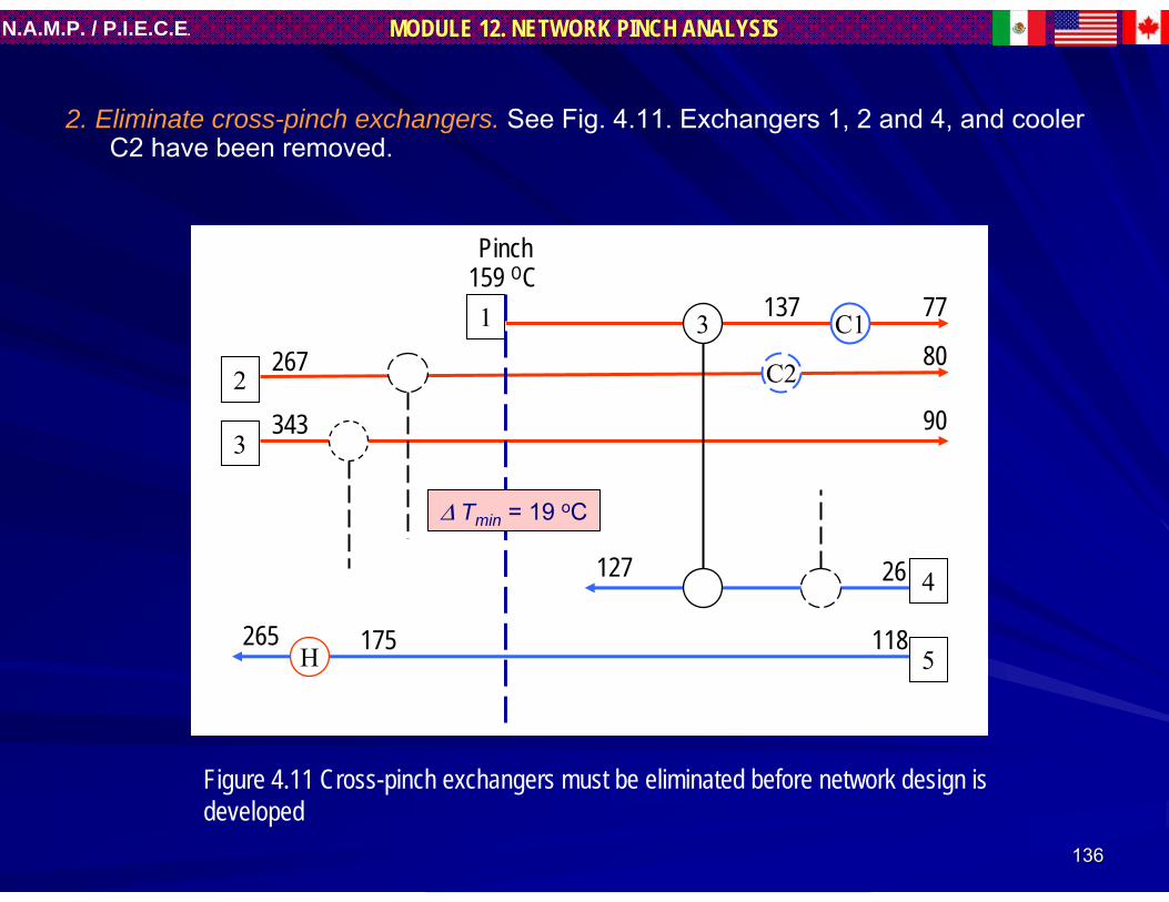
136136
MODULE 12. NETWORK PINCH ANALYSISN.A.M.P. / P.I.E.C.E.
2. Eliminate cross-pinch exchangers. See Fig. 4.11. Exchangers 1, 2 and 4, and cooler C2 have been removed.
1
2
3
4
5
3 C1
H
159 OC137 77
267 80
343 90
26127
118175265
C2
Δ Tmin = 19 oC
Pinch
Figure 4.11 Cross-pinch exchangers must be eliminated before network design is developed

137137
MODULE 12. NETWORK PINCH ANALYSISN.A.M.P. / P.I.E.C.E.
3. Complete the network. Position new exchange exchangers removed in Step 2. A possible network is shown in Fig. 4.12. Above the pinch, the heater and exchangers 1 and 4 are reused. Below the pinch, exchanger 2 is reused, but with reduced duty. The remaining enthalpy on stream 4 is taken by exchanger 3. Cooler C2 has a reduced duty. Exchanger A is new.
Figure 4.12 A preliminary design involves redeploying existing exchangers and adding new units
1
2
3
4
5
3 C1
159 OC115 77
267 80
343 90
26127
118128202265
12,411 4,314
1,612
8,712
9,899
Δ Tmin = 19 oC
3,712
5, 711
140 oC
Pinch
A 140
1 2
2,203
4 C2
H

138138
MODULE 12. NETWORK PINCH ANALYSISN.A.M.P. / P.I.E.C.E.
4. Evolve improvements. Improve compatibility with existing network via heat-load loops and paths. Reuse area of existing exchangers as much as possible.
A loop is a closed connection through streams and exchangers, i.e., it starts and end on the same point on the grid. Consider the corrected network shown in Fig. 4.13. An example loop is indicated by the long-dash line.
Use of loops introduces some flexibility into the design. Suppose the load of the new exchanger A is increased by X units. Then, by enthalpy balance over each, the load on exchanger 3 must be 5,711 – X, that on exchanger 2 will be 3,712 + X, and that on exchanger 1 will be 9,899 – X. This flexibility can be used to make old exchangers fit new duties.
A path also introduce flexibility. It is a connection through streams and exchangers between two utilities. In Fig. 4.13, a path can be traced from the heater through exchanger A to cooler C1 (shown as the short-dash line). Suppose we reduce the heat load on the heater by Y.
By shifting heat loads around loops and along paths, the final network as given in Fig. 4.14 is identified. In this design, the surface area of exchanger 3 is fully reused.
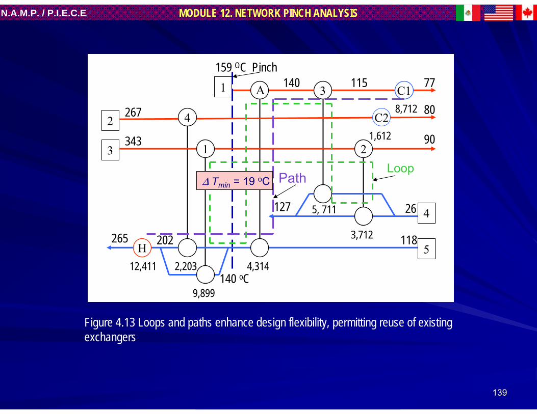
139139
MODULE 12. NETWORK PINCH ANALYSISN.A.M.P. / P.I.E.C.E.
Figure 4.13 Loops and paths enhance design flexibility, permitting reuse of existing exchangers
1
2
3
4
5
3 C1
159 OC115 77
267 80
343 90
26127
118202265
12,411 4,314
1,612
8,712
9,899
3,712
5, 711
140 oC
Pinch
A 140
1 2
2,203
4 C2
H
Δ Tmin = 19 oCLoop
Path
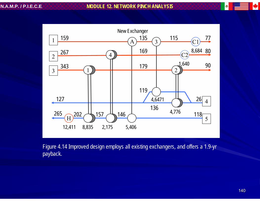
140140
MODULE 12. NETWORK PINCH ANALYSISN.A.M.P. / P.I.E.C.E.
1
2
3
4
5
3 C1115 77
267 80
343 90
26119
118146202265
12,411 5,406
1,640
8,684
8,835
4,776
4,6471
A 135
2,175
C2
H
1
4
22
159New Exchanger
169
179
127136
157
Figure 4.14 Improved design employs all existing exchangers, and offers a 1.9-yr payback.

141141
MODULE 12. NETWORK PINCH ANALYSISN.A.M.P. / P.I.E.C.E.
State-of-the-art retrofit methodology relies on a mixture of past experience with the process, a few technical developments, and some inspired guesses.
The results are retrofit projects that range from ones that pay for themselves within a few weeks, to others that are recognized, soon after installation, to be a hindrance to further improvement.
There always seems to be an element of surprise, much more so than for grassroots design. It seems generally agreed that there is no methodology for the objective prediction of what is possible in a retrofit.

142142
MODULE 12. NETWORK PINCH ANALYSISN.A.M.P. / P.I.E.C.E.
TIER I: FUNDAMENTALSTIER I: FUNDAMENTALS
11 HEAT RECOVERY NETWORKS (HEAT RECOVERY NETWORKS (HENsHENs).).
22 STEADY STATE SIMULATION of STEADY STATE SIMULATION of HENsHENs..
33 OPERABILITY ANALYSIS of OPERABILITY ANALYSIS of HENsHENs..
44 RETROFIT of RETROFIT of HENsHENs..
55 MASS EXCHANGE NETWORKS (MASS EXCHANGE NETWORKS (MENsMENs).).
66 OPERABILITY ANALYSIS of OPERABILITY ANALYSIS of MENsMENs..

143143
MODULE 12. NETWORK PINCH ANALYSISN.A.M.P. / P.I.E.C.E.
5 MASS EXCHANGE NETWORKS.5 MASS EXCHANGE NETWORKS.
5.1 5.1 Introduction.Introduction.
5.2 Synthesis of Mass Exchange Networks.5.2 Synthesis of Mass Exchange Networks.

144144
MODULE 12. NETWORK PINCH ANALYSISN.A.M.P. / P.I.E.C.E.
5.1 INTRODUCTION.5.1 INTRODUCTION.
5.1.1.5.1.1.What is Mass Integration?What is Mass Integration?
5.1.2.5.1.2.TargetingTargeting
5.1.3.5.1.3.Design of individual mass exchangerDesign of individual mass exchanger

145145
MODULE 12. NETWORK PINCH ANALYSISN.A.M.P. / P.I.E.C.E.
5.1.1. What is Mass Integration?5.1.1. What is Mass Integration?ROLE OF PROCESS ENGINEERS IN THE PROCESS INDUSTRIES.
Many process engineers would indicate that their responsibilities in the process industries is to design and operate industrial process and make them work: FASTER, BETTER, CHEAPER, SAFER AND GREENER. All this tasks lead to more competitive processes with desirable profit margins and market share.
KEY DRIVERS FOR PROCESS-ENGINEERING RESEARCH.
These responsibilities may be expressed through to the seven themes identified by Keller and Bryan1 as the key drivers for process-engineering research, development and changes in the primary chemical process industries. These themes are:
Reduction in raw-material cost.
Reduction in capital investment.
Reduction in energy use.
Increase in process flexibility and reduction in inventory.
Ever greater emphasize on process safety.
Better environmental performance.

146146
MODULE 12. NETWORK PINCH ANALYSISN.A.M.P. / P.I.E.C.E.
FACING A TYPICAL CHALLENGING PROCESS IMPROVEMENT PROBLEM.
The following observations may be made facing a typical challenging process improvement problem:
There are typically numerous alternatives that can solve the problem.
The optimum solution may not be intuitively obvious.
One should not focus on the symptoms of the process problem (resulting in solutions as: construct an expansion facility or ever install another one). Instead one should identify the root causes of the process deficiencies (resulting in make in plant process modifications as opposed to “end-of-pipe” solution).
It is necessary to understand and treat the process as an integrated system.
There is a critical need to systematically extract the optimum solution from among the numerous alternatives without enumeration.
CONVENTIONAL ENGINEERING APPROACHES.
Until recently, there were three primary conventional engineering approaches to addressing process development and improvement problems:
1 Brainstorming and solution through scenarios.
2 Adopting/Evolving earlier designs.
3 Heuristics

147147
MODULE 12. NETWORK PINCH ANALYSISN.A.M.P. / P.I.E.C.E.
CONVENTIONAL APPROACHES ENGINEERING HAVE SERIOUS LIMITATIONS.
Notwithstanding the usefulness of these approaches in providing solution that typically work, they have several serious limitations:
Cannot enumerate the infinite alternatives.
Is not guaranteed to come close to optimum solutions.
Time and money intensive.
Limited range of applicability.
Does not shed light on global insights and key characteristics of the process.
Severally limits groundbreaking and novel ideas.
These limitations can be eliminated if these two approaches are incorporated within a systematic and integrative framework
Recent advances in process design have led to the development of systematic, fundamental and generally applicable techniques can be learned and applied to overcome the aforementioned limitations and methodically address process-improvement problems. This is possible through PROCESS INTEGRATION.PROCESS INTEGRATION.

148148
MODULE 12. NETWORK PINCH ANALYSISN.A.M.P. / P.I.E.C.E.
PROCESS INTEGRATIONPROCESS INTEGRATION
Process Integration is a holistic approach to process design, reProcess Integration is a holistic approach to process design, retrofitting and trofitting and operation which emphasizes the unity of the processoperation which emphasizes the unity of the process22..
Process Integration involves the following activities:Process Integration involves the following activities:
1 TASK IDENTIFICATION.1 TASK IDENTIFICATION.
2 TARGETING2 TARGETING
3 GENERATION OF ALTERNATIVES.3 GENERATION OF ALTERNATIVES.
4 SELECTION OF ALTERNATIVES.4 SELECTION OF ALTERNATIVES.
5 ANALYSIS OF SELECTED ALTERNATIVES.5 ANALYSIS OF SELECTED ALTERNATIVES.
CLASIFICATION OF PROCESS INTEGRATIONCLASIFICATION OF PROCESS INTEGRATION..
From the perspective of resource integration, process integration may be classified into:
ENERGY INTEGRATION
MASS INTEGRATION

149149
MODULE 12. NETWORK PINCH ANALYSISN.A.M.P. / P.I.E.C.E.
FINALLY, WHAT IS MASS INTEGRATION?
Mass Integration is a systematic methodology that provides a fundamental understanding of the global flow of mass within the process and employs this understanding in identifying performance target and optimizing the generation and routing of species throughout the process.
Mass-allocation objectives such a pollution prevention are the heart of mass integration.
Mass integration is based on fundamental principles of chemical engineering combined with systematic analysis using graphical and optimization-based tools.
The first step in conducting mass integration is the development of a global mass allocation representation of the whole process from a species viewpoint (Fig. 5.1):
Targeted species: e.g. pollutant, valuable material.Sources: stream that carry the species (Rich streams)Sinks: units that can accept the species (Reactors, heaters, coolers,
bio-treatment facilities, and discharge media).Mass Separating Agents (MSAs): Solvents, adsorbents, etc.
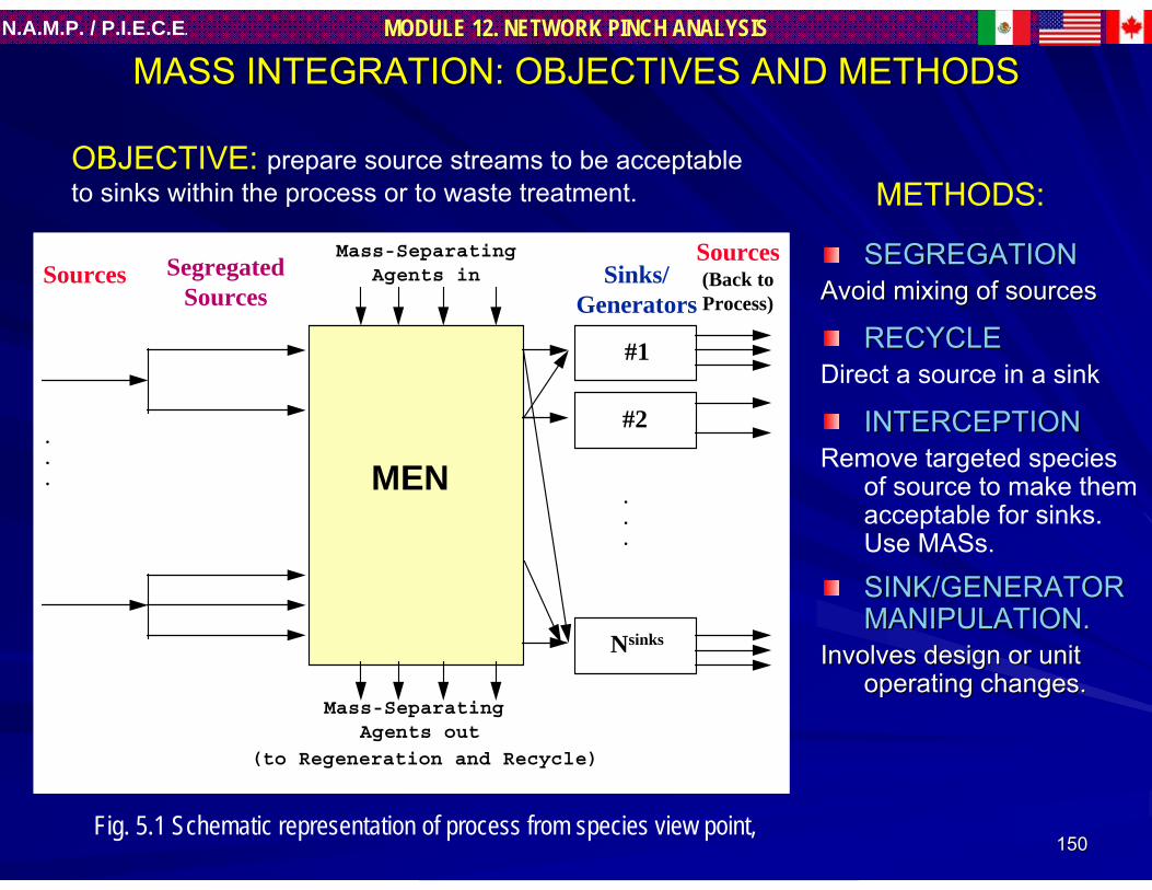
150150
MODULE 12. NETWORK PINCH ANALYSISN.A.M.P. / P.I.E.C.E.
Mass-Separating Agents in
Mass-Separating Agents out
(to Regeneration and Recycle)
.
.
.
#1
#2
Nsinks
.
.
.
Sources SegregatedSources
Sinks/Generators
Sources(Back toProcess)
MEN
MASS INTEGRATION: OBJECTIVES AND METHODSMASS INTEGRATION: OBJECTIVES AND METHODS
OBJECTIVE: prepare source streams to be acceptableto sinks within the process or to waste treatment. METHODS:
SEGREGATIONSEGREGATIONAvoid mixing of sourcesAvoid mixing of sources
RECYCLERECYCLEDirect a source in a sink
INTERCEPTIONINTERCEPTIONRemove targeted species
of source to make them acceptable for sinks. Use MASs.
SINK/GENERATOR SINK/GENERATOR MANIPULATION.MANIPULATION.
Involves design or unit Involves design or unit operating changes. operating changes.
Fig. 5.1 Schematic representation of process from species view point,
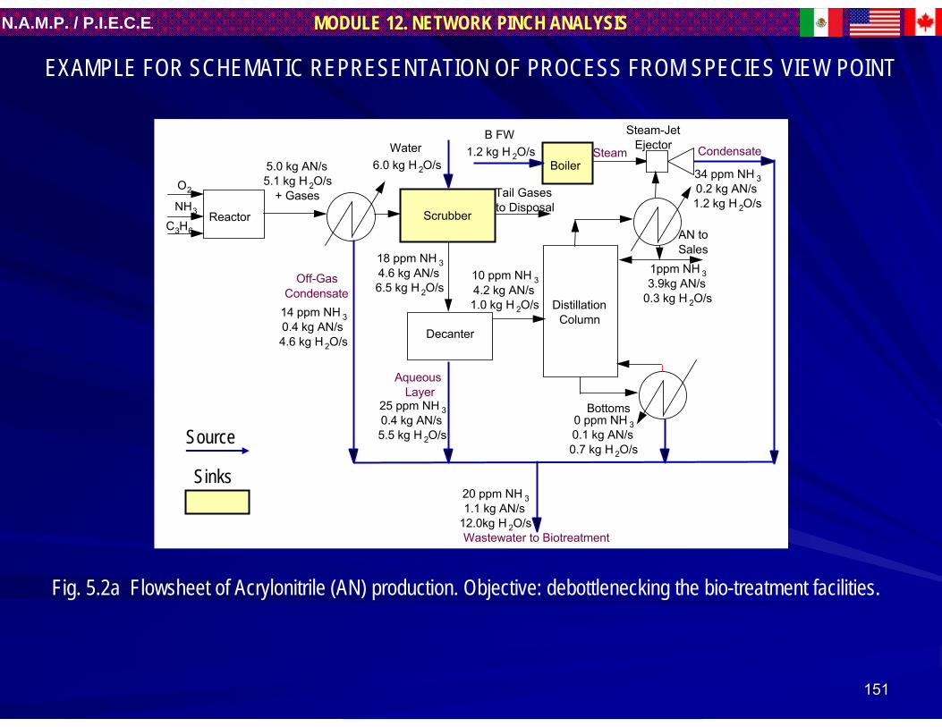
151151
MODULE 12. NETWORK PINCH ANALYSISN.A.M.P. / P.I.E.C.E.
O2
Decanter
DistillationColumn
Aqueous Layer
Reactor ScrubberNH3
C3H6
Steam-JetEjector
Steam
Wastewater to Biotreatment
Off-GasCondensate
Condensate
Bottoms
Water
AN toSales
6.0 kg H 2O/s
14 ppm NH 30.4 kg AN/s4.6 kg H 2O/s
25 ppm NH 30.4 kg AN/s5.5 kg H 2O/s
34 ppm NH 30.2 kg AN/s1.2 kg H 2O/s
18 ppm NH 34.6 kg AN/s6.5 kg H 2O/s
10 ppm NH 34.2 kg AN/s1.0 kg H 2O/s
5.0 kg AN/s5.1 kg H 2O/s
+ Gases
20 ppm NH 31.1 kg AN/s
12.0kg H 2O/s
Tail Gases to Disposal
B FW1.2 kg H 2O/s
Boiler
0 ppm NH 30.1 kg AN/s0.7 kg H 2O/s
1ppm NH 33.9kg AN/s
0.3 kg H 2O/s
Source
Sinks
EXAMPLE FOR SCHEMATIC REPRESENTATION OF PROCESS FROM SPECIES VIEW POINT
Fig. 5.2a Flowsheet of Acrylonitrile (AN) production. Objective: debottlenecking the bio-treatment facilities.
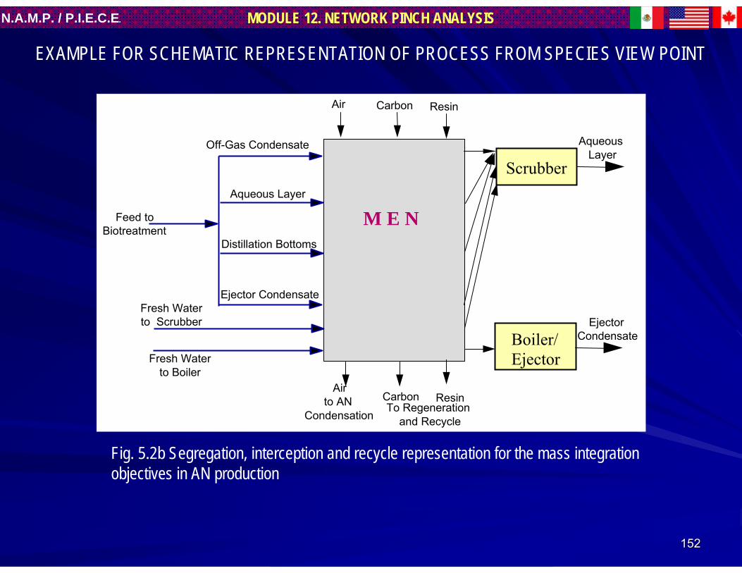
152152
MODULE 12. NETWORK PINCH ANALYSISN.A.M.P. / P.I.E.C.E.
M E N
Scrubber
Boiler/Ejector
Air Carbon Resin
Airto AN
Condensation
Carbon ResinTo Regeneration
and Recycle
Feed toBiotreatment
Off-Gas Condensate
Aqueous Layer
Distillation Bottoms
Ejector Condensate
Aqueous Layer
Ejector Condensate
Fresh Waterto Boiler
Fresh Waterto Scrubber
EXAMPLE FOR SCHEMATIC REPRESENTATION OF PROCESS FROM SPECIES VIEW POINT
Fig. 5.2b Segregation, interception and recycle representation for the mass integrationobjectives in AN production

153153
MODULE 12. NETWORK PINCH ANALYSISN.A.M.P. / P.I.E.C.E.
5.1 INTRODUCTION.5.1 INTRODUCTION.
5.1.1.5.1.1.What is Mass Integration?What is Mass Integration?
5.1.2.5.1.2.TargetingTargeting
5.1.3.5.1.3.Design of individual mass exchangerDesign of individual mass exchanger

154154
MODULE 12. NETWORK PINCH ANALYSISN.A.M.P. / P.I.E.C.E.
5.1.2. TARGETING5.1.2. TARGETING
OVERALL MASS TARGETING
In many cases, it is useful to determine the potential improvement in the performance of a whole process or sections of the process without actually developing the
details of the solution. In this context, the concept of targeting is very useful.
THE TARGETING APPROACH
Based on identification of performance targets ahead of design and without prior commitment to the final network
configuration.

155155
MODULE 12. NETWORK PINCH ANALYSISN.A.M.P. / P.I.E.C.E.
TARGETS FOR TARGETS FOR MENsMENs SYNTHESISSYNTHESIS..
1.- MINIMUM COST OF MSAsSince the cost of MSAs is typically the dominant operating expenses,this target is aimed at minimizing the operating cost of the MEN,Any design featuring the minimum cost of MSAs will be referred to as a minimum operating cost (MOC) solution.
2.2.-- MINIMUM NUMBER OFMASS EXCHANGER UNITS.MINIMUM NUMBER OFMASS EXCHANGER UNITS.This objective attempts to minimize indirectly the This objective attempts to minimize indirectly the fixed costfixed cost of the network. of the network. Minimizing the Minimizing the number of separatorsnumber of separators ((U) so as to reduce so as to reduce pipeworkpipework, foundations, , foundations, maintenance, and instrumentationmaintenance, and instrumentation..
U = NU = NRR + N+ NSS -- NNii
NNR R = Number of Rich streams,NNSS = Number of MSAs
In general, these two targets are incompatible. Systematic techniques will be presented to enable the identifying an MOC solution and the minimizing the number of exchangers satisfying the MOC.
Number of independent synthesis subproblems into which the original synthesis problem can be subdivided. Usually Ni = 1
(5.1)

156156
MODULE 12. NETWORK PINCH ANALYSISN.A.M.P. / P.I.E.C.E.
5.1 INTRODUCTION5.1 INTRODUCTION..
5.1.1.5.1.1.What is Mass Integration?What is Mass Integration?
5.1.2.5.1.2.TargetingTargeting
5.1.3.5.1.3.Design of individual mass exchangerDesign of individual mass exchanger
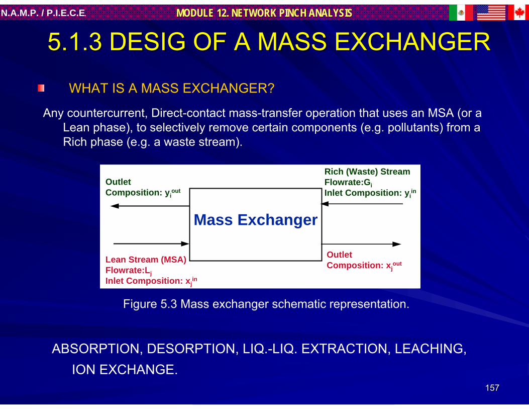
157157
MODULE 12. NETWORK PINCH ANALYSISN.A.M.P. / P.I.E.C.E.
Any countercurrent, Direct-contact mass-transfer operation that uses an MSA (or a Lean phase), to selectively remove certain components (e.g. pollutants) from a Rich phase (e.g. a waste stream).
ABSORPTION, DESORPTION, LIQ.-LIQ. EXTRACTION, LEACHING, ION EXCHANGE.
WHAT IS A MASS EXCHANGER?
5.1.3 DESIG OF A MASS EXCHANGER5.1.3 DESIG OF A MASS EXCHANGER
Mass Exchanger
Outlet Composition: yi
out
Lean Stream (MSA) Flowrate:Lj Inlet Composition: xj
in
Outlet Composition: xj
out
Rich (Waste) StreamFlowrate:Gi Inlet Composition: yi
in
Figure 5.3 Mass exchanger schematic representation.

158158
MODULE 12. NETWORK PINCH ANALYSISN.A.M.P. / P.I.E.C.E.
EQUILIBRIUMEQUILIBRIUM
Generalized description.Generalized description.The composition of the Rich stream (yi) is a function of the composition of the Lean stream (xj)
yi = f*(xj*)
Dilute SystemDilute SystemFor some applications the equilibrium function may be For some applications the equilibrium function may be linearizedlinearized over the operating over the operating range.range.
yyii = = mmjj··xx**jj + + bbjj
InterphaseInterphase Mass transferMass transferFor linear equilibrium the pollutant composition in the lean phase in equilibrium yi can be calculated by
For linear equilibrium the pollutant composition in the rich phase in equilibrium xj can be calculated by
* i jj
j
y bx
m−
=
*i j j jy m x b= ⋅ +
(5.2)
(5.3)
(5.4)
(5.5)

159159
MODULE 12. NETWORK PINCH ANALYSISN.A.M.P. / P.I.E.C.E.
Special casesSpecial cases–– RaoultRaoult’’ss Law for absorption:Law for absorption:
–– HenryHenry’’s Law for stripings Law for striping
– Distribution function used in solvent extraction
yi = Kj·x*j
EQUILIBRIUMEQUILIBRIUM
0*( )solute
i jTotal
p Ty xP
= ⋅
*i j jy H x= ⋅
solubility0 ( )
( )Total
j isolute
PH y Tp T
= ⋅
yi Mole fraction of solute in gas
Posolute Vapor pressure of solute at T
x*j Mole fraction of solute in liquid
PTotal Total pressure of gas
yi Mole fraction of solute in gas
x*j Mole fraction of solute in liquid
Hj Henry’s coefficient
yisolubility Liquid-phase solubility of
the pollutant at temperature T
Kj Distribution Coefficient
(5.6)
(5.7)
(5.8)
(5.9)

160160
MODULE 12. NETWORK PINCH ANALYSISN.A.M.P. / P.I.E.C.E.
MASS EXCHANGER MODELING: MASS EXCHANGER MODELING: MULTISTAGE CONTACTORSMULTISTAGE CONTACTORS
Light Phase Out
Heavy Phase In
Light Phase In
Heavy Phase Out
Shell
PerforatedPlate (Tray)
Weir
Downcomer
MSA out
Waste in MSA
in
Waste out
Fig. 5.4 A multistage tray column Fig. 5.5 A three-stage mixer-setter system
EXAMPLES OF MULTISTAGES CONTACTORSEXAMPLES OF MULTISTAGES CONTACTORS

161161
MODULE 12. NETWORK PINCH ANALYSISN.A.M.P. / P.I.E.C.E.
A GENERIC MASS EXCHANGER
SCHEMATIC OF A MULTISTAGE MASS EXCHANGER
MASS EXCHANGER MODELING: MASS EXCHANGER MODELING: MULTISTAGE CONTACTORSMULTISTAGE CONTACTORS
Mass Exchanger
Outlet Composition: yi
out
Lean Stream (MSA) Flowrate:Lj Inlet Composition: xj
in
Outlet Composition: xj
out
Rich (Waste) StreamFlowrate:Gi Inlet Composition: yi
in
1 2 n N-1 N
yi,1=yiout
xj,0=xjin xj,1
xj,2
yi,2 yi,3 yi,n
xj,n.1 xj,n
yi,n+1 yi,N-1 yi,N
xj,N-2 xj,N-1 xj,N=xjout
yi,N+1=yiin
Figure 5.3 Mass exchanger schematic representation.
Fig. 5.6 A schematic diagram of a multistage mass exchanger

162162
MODULE 12. NETWORK PINCH ANALYSISN.A.M.P. / P.I.E.C.E.
MASS EXCHANGER MODELING: MASS EXCHANGER MODELING: MULTISTAGE CONTACTORSMULTISTAGE CONTACTORS
OPERATING LINE (MATERIAL BALANCE)
THE THE McCABEMcCABE--THIELE DIAGRAMTHIELE DIAGRAM
yout xin
yin xout
L
G
yiin
y iout
x jin x j
out
x j
y i
O perating L ine
Equilibrium Line
L j/G i
)injxout
j(xjL)outiyin
i(yiG −=−
Figure 5.7 The McCabe Thiele diagram

163163
MODULE 12. NETWORK PINCH ANALYSISN.A.M.P. / P.I.E.C.E.
THE KREMSER EQUATION:THE KREMSER EQUATION:For the case of isothermal, dilute mass exchanger with linear equilibrium, the Number of Theoretical Plates (NTP)for a mass exchanger can be determined through the Kremser equation:
MASS EXCHANGER MODELING:MASS EXCHANGER MODELING: MULTISTAGE CONTACTORSMULTISTAGE CONTACTORS
ln 1
ln
in inj i i j j j j i
out inj i j j j j
j
j i
m G y m x b m GL y m x b L
NTPL
m G
⎡ ⎤⎛ ⎞⎛ ⎞− −− +⎢ ⎥⎜ ⎟⎜ ⎟⎜ ⎟⎜ ⎟− −⎢ ⎥⎝ ⎠⎝ ⎠⎣ ⎦=
⎛ ⎞⎜ ⎟⎜ ⎟⎝ ⎠
(5.10)

164164
MODULE 12. NETWORK PINCH ANALYSISN.A.M.P. / P.I.E.C.E.
OTHER FORM OF KREMSER EQUATION IS
also
where
,*
,*ln 1
ln
in outj i j i
out outj i j j j i
j i
j
L x x Lm G x x m G
NTPm G
L
⎡ ⎤⎛ ⎞⎛ ⎞−− +⎢ ⎥⎜ ⎟⎜ ⎟⎜ ⎟⎜ ⎟−⎢ ⎥⎝ ⎠⎝ ⎠⎣ ⎦=
⎛ ⎞⎜ ⎟⎜ ⎟⎝ ⎠
MASS EXCHANGER MODELING: MASS EXCHANGER MODELING: MULTISTAGE CONTACTORSMULTISTAGE CONTACTORS
,*ini jout
jj
y bx
m−
=
NTPin outi j j j jout ini j j j j i
y m x b Ly m x b m G
⎛ ⎞− −= ⎜ ⎟⎜ ⎟− − ⎝ ⎠
(5.11)
(5.12)
(5.13)

165165
MODULE 12. NETWORK PINCH ANALYSISN.A.M.P. / P.I.E.C.E.
NUMBER OF ACTUAL PLATES (NAP)NUMBER OF ACTUAL PLATES (NAP)The overall exchanger efficiency, η0 , can be used to relate NAP and NTP as follows
The Stage efficiency can be based on either the rich or the leanThe Stage efficiency can be based on either the rich or the lean phase. If based on phase. If based on the rich phase the the rich phase the KremserKremser equation can rewritten asequation can rewritten as
MASS EXCHANGER MODELING: MASS EXCHANGER MODELING: MULTISTAGE CONTACTORSMULTISTAGE CONTACTORS
o
NTPNAPη
=
ln 1
ln 1 1
in inj i i j j j j i
out inj i j j j j
j iy
j
m G y m x b m GL y m x b L
NTPm G
Lη
⎡ ⎤⎛ ⎞⎛ ⎞− −− +⎢ ⎥⎜ ⎟⎜ ⎟⎜ ⎟⎜ ⎟− −⎢ ⎥⎝ ⎠⎝ ⎠⎣ ⎦=
⎧ ⎫⎡ ⎤⎛ ⎞⎪ ⎪− + −⎢ ⎥⎜ ⎟⎨ ⎬⎜ ⎟⎢ ⎥⎪ ⎪⎝ ⎠⎣ ⎦⎩ ⎭
(5.14)
(5.15)

166166
MODULE 12. NETWORK PINCH ANALYSISN.A.M.P. / P.I.E.C.E.
MASS EXCHANGER MODELING:MASS EXCHANGER MODELING:DIFFERENTIAL (or CONTINUOS) CONTACTORSDIFFERENTIAL (or CONTINUOS) CONTACTORS
Light Phase in
Heavy Phase In
Packing Restrainer
Random Packing
Heavy-Phase Re-Distributor
Heavy Phase Out
Packing Support
Shell
Light Phase Out
Random Packing
Light Phase Out
Heavy Phase In
Light Phase In
Heavy Phase Out
Shell
Figure 5.8 Counter current packedcolumn
5.10 A spray column
Light Phase Out
Heavy Phase In
Light Phase In
Heavy Phase Out
Shell
Mixer
Figure 5.9 A mechanically-agitatedmass exchanger
EXAMPLES OF DIFFERENTIALS CONTACTORSEXAMPLES OF DIFFERENTIALS CONTACTORS

167167
MODULE 12. NETWORK PINCH ANALYSISN.A.M.P. / P.I.E.C.E.
HEIGH OF A DIFFERENTIAL CONTACTOR, HEIGH OF A DIFFERENTIAL CONTACTOR, HH..
where HTUy and HTUx are the overall height of transfer units based on the rich and the lean phases, respectively, while, NTUy and NTUx are the overall number of transfer units based on the rich and lean phases, respectively
MASS EXCHANGER MODELINGMASS EXCHANGER MODELINGDIFFERENTIAL (or CONTINUOS) CONTACTORSDIFFERENTIAL (or CONTINUOS) CONTACTORS
y yH HTU NTU=
x xH HTU NTU=
(5.14)
(5.15)

168168
MODULE 12. NETWORK PINCH ANALYSISN.A.M.P. / P.I.E.C.E.
EQUATION FOR EQUATION FOR NTUNTUyy
For the case of isothermal, dilute mass exchanger with linear eqFor the case of isothermal, dilute mass exchanger with linear equilibrium the uilibrium the NTUNTUyycan be theoretically estimated as followcan be theoretically estimated as follow
wherewhere
MASS EXCHANGER MODELINGMASS EXCHANGER MODELINGDIFFERENTIAL (or CONTINUOS) CONTACTORSDIFFERENTIAL (or CONTINUOS) CONTACTORS
*log( )
in outi i
yi i mean
y yNTUy y
−=−
( ) ( ) ( )*
log
ln
in out out ini j j j i j j j
i i in outmeani j j jout ini j j j
y m x b y m x by y
y m x by m x b
− − − − −− =
⎛ ⎞− −⎜ ⎟⎜ ⎟− −⎝ ⎠
(5.16)
(5.17)

169169
MODULE 12. NETWORK PINCH ANALYSISN.A.M.P. / P.I.E.C.E.
MASS EXCHANGER MODELINGMASS EXCHANGER MODELINGDIFFERENTIAL (or CONTINUOS) CONTACTORSDIFFERENTIAL (or CONTINUOS) CONTACTORS
EQUATION FOR EQUATION FOR NTUNTUxx
For the case of isothermal, dilute mass exchanger with linear eqFor the case of isothermal, dilute mass exchanger with linear equilibrium the uilibrium the NTUNTUxx can be theoretically estimated as followcan be theoretically estimated as follow
wherewhere meanjj
outj
inj
x xxxx
NTUlog
* )( −−
=
⎪⎪
⎭
⎪⎪
⎬
⎫
⎪⎪
⎩
⎪⎪
⎨
⎧
⎥⎥⎦
⎤
⎢⎢⎣
⎡⎟⎟⎠
⎞⎜⎜⎝
⎛ −−
⎥⎥⎦
⎤
⎢⎢⎣
⎡⎟⎟⎠
⎞⎜⎜⎝
⎛ −−
⎥⎥⎦
⎤
⎢⎢⎣
⎡⎟⎟⎠
⎞⎜⎜⎝
⎛ −−−
⎥⎥⎦
⎤
⎢⎢⎣
⎡⎟⎟⎠
⎞⎜⎜⎝
⎛ −−
=−
j
joutiin
j
j
jiniout
j
j
joutiin
jj
jiniout
j
meanjj
mby
x
mby
x
mby
xm
byx
xx
ln
)( log*
(5.18)
(5.19)

170170
MODULE 12. NETWORK PINCH ANALYSISN.A.M.P. / P.I.E.C.E.
COLUMN DIAMETER COLUMN DIAMETER
The column diameter is normally determined by selecting a superficial velocity for one (or both) of the phases. This velocity is intended to ensure proper mixing while avoiding hydrodynamic problems such as flooding, weeping, or entrainment.
Once a superficial velocity is determined, the cross-sectional area of the column is obtained by dividing the volumetric flowrate by the velocity.
MASS EXCHANGER MODELINGMASS EXCHANGER MODELING

171171
MODULE 12. NETWORK PINCH ANALYSISN.A.M.P. / P.I.E.C.E.
TOTAL ANUALIZED COST (TAC)TOTAL ANUALIZED COST (TAC)
WHICH CAR IS CHEAPER?WHICH CAR IS CHEAPER?
1978
Wait! Don’t answer yet.
2005

172172
MODULE 12. NETWORK PINCH ANALYSISN.A.M.P. / P.I.E.C.E.
FIXED COSTFIXED COSTThe car itself, i.e. body, engine, tires, etc.Old car: $ 500.00New car: $21,000.00
ANNUAL OPERATING COST (AOC)ANNUAL OPERATING COST (AOC)How much to run and maintain the car.Old car: $ 4,000.00/yearNew car: $ $ 700.00/year.
TOTAL ANUALIZED COST (TAC)TOTAL ANUALIZED COST (TAC)
We need to annualize the
Fixed Costof the car
Fixed Cost >>$vs
AOC >> $/year !!!!

173173
MODULE 12. NETWORK PINCH ANALYSISN.A.M.P. / P.I.E.C.E.
ANNUALIZED FIXED COST (AFC)ANNUALIZED FIXED COST (AFC)
TOTAL ANNUALIZED COST (TAC)TOTAL ANNUALIZED COST (TAC)
TOTAL ANUALIZED COST (TAC)TOTAL ANUALIZED COST (TAC)
Initial Fixed Cost Salvage or Resale ValueAFCUseful Life Period
−=
TAC Annualized Fixed Cost Annual Operating Cost= +
(5.20)
(5.21)

174174
MODULE 12. NETWORK PINCH ANALYSISN.A.M.P. / P.I.E.C.E.
Useful life: 2 yearsSalvage value: $ 200.00
AFC = ($ 500 - $ 200)/2 yr AFC = $ 150/yr
TOTAL ANUALIZED COST (TAC)TOTAL ANUALIZED COST (TAC)
Useful life: 20 yearsSalvage value: $ 1000
AFC = ( $ 21000 - $ 1000)/20 yrAFC = $ 1000/yr

175175
MODULE 12. NETWORK PINCH ANALYSISN.A.M.P. / P.I.E.C.E.
TAC = $ 4,000 + $ 250 TAC = $ 1,000 + $ 700
TOTAL ANUALIZED COST (TAC)TOTAL ANUALIZED COST (TAC)

176176
MODULE 12. NETWORK PINCH ANALYSISN.A.M.P. / P.I.E.C.E.
MINIMIZING COST OF MASS EXCHANGE SYSTEMSMINIMIZING COST OF MASS EXCHANGE SYSTEMS
TOTAL ANNUALIZED COSTTOTAL ANNUALIZED COST– Fixed Cost: Trays. Shell. Packing, etc.– Operating Cost: Solvent makeup, pumping, heating, cooling,etc.
DRIVING FORCEDRIVING FORCE– Minimum Allowed
Composition Difference (ε).– Must stay to left of
equilibrium line.
TAC AOC AFC= +
xj
EquilibriumLine
y
ε j
ε j
Practical Feasibility Region
Practical Feasibility Line
x*j = (y - bj )/mj
(5.22)
Figure 5.11 Establishing correspondingcomposition scales.
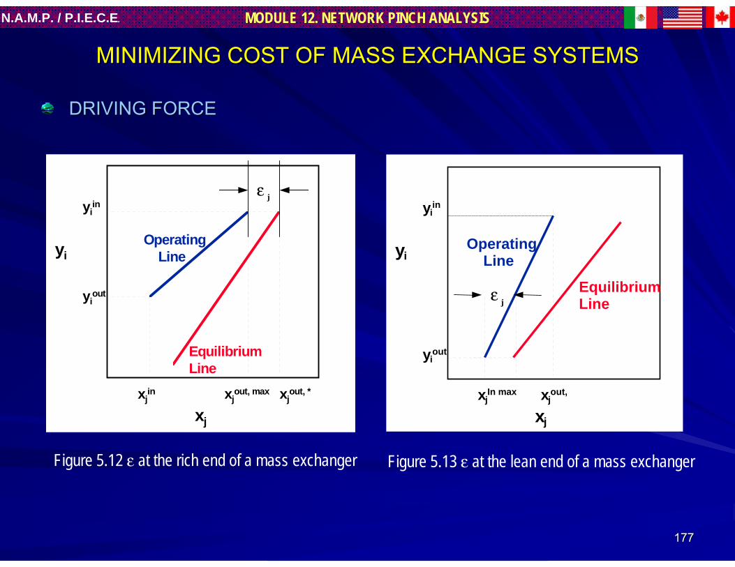
177177
MODULE 12. NETWORK PINCH ANALYSISN.A.M.P. / P.I.E.C.E.
DRIVING FORCEDRIVING FORCE
MINIMIZING COST OF MASS EXCHANGE SYSTEMSMINIMIZING COST OF MASS EXCHANGE SYSTEMS
xjout, max xj
out, *xjin
yiout
yiin
Operating Line
EquilibriumLine
xj
yi
ε j
Figure 5.12 ε at the rich end of a mass exchanger Figure 5.13 ε at the lean end of a mass exchanger
xjout, xj
In max
yiout
yiin
OperatingLine
EquilibriumLine
xj
yi
ε j

178178
MODULE 12. NETWORK PINCH ANALYSISN.A.M.P. / P.I.E.C.E.
MINIMIZING COST OF MASS EXCHANGE SYSTEMSMINIMIZING COST OF MASS EXCHANGE SYSTEMS
DRIVE FORCEε at the rich end of mass exchanger.
but
Combining Eqs. (5.23) and (5.24), one obtains
joutj
outj xx ε−= ,*max,
When the minimum allowable composition difference εj
increases, then the ratio of L/G increases.
AOC increases, due to higher MSA flow
AFC decreases, due to smaller equipment, e.g.
fewer stages
joutjj
ini bxmy += ,*
jj
jin
outj m
byx ε−
−=max,
(5.23)
(5.24)
(5.25)

179179
MODULE 12. NETWORK PINCH ANALYSISN.A.M.P. / P.I.E.C.E.
DRIVING FORCE OPTIMUMDRIVING FORCE OPTIMUM
MINIMIZING COST OF MASS EXCHANGE SYSTEMSMINIMIZING COST OF MASS EXCHANGE SYSTEMS
0.0020 0.0030 0.0040 0.0050
0
10,000
20,000
30,000
40,000
50,000
60,000
70,000
0.0000 0.0010
ε
$/ye
ar
TAC
Annual Operating Cost
Annualized Fixed Cost
Minimum Allowable Composition Difference,
Trade-off between reducing fixed cost and increasing
operating cost
Composition driving force, becomes a optimization variable
O P T I MU M
Figure 5.14 Using mass transfer force to trade off fixed cost versusoperating cost.

180180
MODULE 12. NETWORK PINCH ANALYSISN.A.M.P. / P.I.E.C.E.
5 MASS EXCHANGE NETWORKS.5 MASS EXCHANGE NETWORKS.
5.1 5.1 Introduction.Introduction.
5.2 Synthesis of Mass Exchange Networks.5.2 Synthesis of Mass Exchange Networks.

181181
MODULE 12. NETWORK PINCH ANALYSISN.A.M.P. / P.I.E.C.E.
5.2 SYNTHESIS of MASS EXCHANGER 5.2 SYNTHESIS of MASS EXCHANGER NETWORKSNETWORKS
5.2.1 Problem statement5.2.1 Problem statement..
5.2.2 Graphical approach: Mass Exchange 5.2.2 Graphical approach: Mass Exchange Diagram.Diagram.
5.2.3 Algebraic approach: Composition 5.2.3 Algebraic approach: Composition Interval Diagram.Interval Diagram.
5.2.4 Network Synthesis5.2.4 Network Synthesis

182182
MODULE 12. NETWORK PINCH ANALYSISN.A.M.P. / P.I.E.C.E.
SYNTHESIS OF MASS ECHANGE NETWORKS (SYNTHESIS OF MASS ECHANGE NETWORKS (MENsMENs))
WHAT MEAN WHAT MEAN ““MENsMENs”” SYNTHESIS?SYNTHESIS?
By By ““MENsMENs SynthesisSynthesis””, we mean the synthesis generation of , we mean the synthesis generation of
a costa cost--effective network of mass exchangers with the effective network of mass exchangers with the
purpose of preferentially transferring certain species from purpose of preferentially transferring certain species from
a set of rich stream to a set of lean streama set of rich stream to a set of lean stream..

183183
MODULE 12. NETWORK PINCH ANALYSISN.A.M.P. / P.I.E.C.E.
CHEMICAL
PETROLEUM
GAS
PETROCHEMICAL
PHARMACEUTICAL
FOOD
MICROELECTRONICS
METAL
TEXTILE
FORESTRY PRODUCTS
SYNTHESIS OF MASS ECHANGE NETWORKS SYNTHESIS OF MASS ECHANGE NETWORKS ((MENsMENs))
INDUSTRY CANDIDATES TO USE OF MENs

184184
MODULE 12. NETWORK PINCH ANALYSISN.A.M.P. / P.I.E.C.E.
5.1.1 PROLEM ESTATEMENT5.1.1 PROLEM ESTATEMENT
MassExchange Network
MSA’s (Lean Streams In)
RichStreamsIn
RichStreamsOut
MSA’s (Lean Streams Out)
Figure 5.15 Schematic representation of the MEN synthesis problem

185185
MODULE 12. NETWORK PINCH ANALYSISN.A.M.P. / P.I.E.C.E.
WHAT DO WE KNOW?WHAT DO WE KNOW?A Number of NR of waste (rich streams) sources.A Number of Mass Separation Agents (lean streams) NS = NSP + NSE:
• NSP Number of of process MSAs• NSE Number of of external MSAs
Flowrate of of each waste stream, Gi, its supply (inlet) composition, ysi and its
target (outlet) composition, yti, where i = 1, 2 ,…NR
The supply and target compositions, xsj , and, xt
j , for each MSA, where j = 1, 2, …., NS.
WHAT DONWHAT DON’’T WE KNOW?T WE KNOW?The flowrate of each MSA is unknown and is to be determined so as to minimize the network cost.

186186
MODULE 12. NETWORK PINCH ANALYSISN.A.M.P. / P.I.E.C.E.
CONSTRAINTS FOR EACH LEAN STREAM (CONSTRAINTS FOR EACH LEAN STREAM (MSAsMSAs).).
Target CompositionPHYSICAL e.g. maximum solubility of solute in solvent.
ECONOMIC to optimize the cost of any subsequent separation of the effluent lean stream.
TECHNICAL to avoid excessive corrosion, viscosity, or fouling.
ENVIRONMENTAL as imposed by some environmental protection regulation.
FlowrateThe lean process streams already exist at plant site and are bounded by availability in the plant. Can be used for pollutant removal for virtually free.
The mass flow rate of any external MSA is flexible and should be determined according to the economic considerations of the networks synthesis.
PROLEM ESTATEMENTPROLEM ESTATEMENT

187187
MODULE 12. NETWORK PINCH ANALYSISN.A.M.P. / P.I.E.C.E.
BASIC ASSUMPTIONS.
1 The flowrate of each stream remains essentially unchanged as it passes through network.
Gini = Gout
i
Linj = Lout
j
2 Within the MEN, stream recycling is not allowed.
3 In the range of composition involved, any equilibrium relation governing the distribution of a targeted species between the rich stream and the lean stream is linear and independent of the presence of othe soluble components in the rich stream.
yi = mj·x*j + bj
where both mj and bj are assumed to be constants.
PROLEM ESTATEMENTPROLEM ESTATEMENT
(5.26)
(5.27)
(5.28)

188188
MODULE 12. NETWORK PINCH ANALYSISN.A.M.P. / P.I.E.C.E.
MEN SYNTHESIS TASKMEN SYNTHESIS TASK..– Which mass-exchange operations should be used (e.g. absorption, adsorption)?
– Which MSAs should be selected (e.g. which solvents, adsorbents)?
– What is the optimal flowrate of each MSA?
– How should these MSAs be matched with the waste streams (I.e., stream pairings)?
–– What is the optimal system configuration (e.g., how should theseWhat is the optimal system configuration (e.g., how should these mass mass exchangers be arranged? Is there any stream splitting and mixingexchangers be arranged? Is there any stream splitting and mixing?)??)?
PROBLEM ESTATEMENTPROBLEM ESTATEMENT

189189
MODULE 12. NETWORK PINCH ANALYSISN.A.M.P. / P.I.E.C.E.
DESIGN TAGETSDESIGN TAGETSMinimum Cost of MSAsThis target aims at minimizing the operating cost of the network. In many industrial applications, this target has a profound impact on the economics of the separation system.
Minimum Number of Mass Exchamger Units.This objective attempts to minimize indirectly the fixed cost of the network since the cost of each mass exchanger is usually a cocave function of the unit size.
PROBLEM ESTATEMENTPROBLEM ESTATEMENT

190190
MODULE 12. NETWORK PINCH ANALYSISN.A.M.P. / P.I.E.C.E.
5.2 SYNTHESIS of MASS EXCHANGER 5.2 SYNTHESIS of MASS EXCHANGER NETWORKSNETWORKS
5.2.1. Problem statement.5.2.1. Problem statement.
5.2.2. Graphical approach: Mass Exchange Diagram.5.2.2. Graphical approach: Mass Exchange Diagram.5.2.3. Algebraic approach: Composition Interval 5.2.3. Algebraic approach: Composition Interval
Diagram.Diagram.5.2.4 Design for Minimum Number of Mass 5.2.4 Design for Minimum Number of Mass
Exchanger Units.Exchanger Units.

191191
MODULE 12. NETWORK PINCH ANALYSISN.A.M.P. / P.I.E.C.E.
5.2.2 GRAPHICAL APPROACH: MASS EXCHANGE 5.2.2 GRAPHICAL APPROACH: MASS EXCHANGE DIAGRAMDIAGRAM
THE CORRESPONDING COMPOSITION SCALES.
The concept of “corresponding composition scales” is a tool for incorporating constraints of mass exchange by establishing a one-to-one correspondence among the composition of all streams for which mass transfer is thermodynamically feasible.
This concept is based on a generalization of the notion of a “minimum allowable composition difference’, ε, presented before.

192192
MODULE 12. NETWORK PINCH ANALYSISN.A.M.P. / P.I.E.C.E.
The equilibrium relation governing the transfer of the pollutant from the waste stream, ,to the MSA, , is t given by the linear equation (5.28)
which indicates that for a waste stream composition of, , the maximum theoretically attainable composition of the MSA is .
*i j j jy m x b= ⋅ +
xj
EquilibriumLine
y
ε j
ε j
Practical Feasibility Region
Practical Feasibility Line
x*j = (y - bj )/mj
The mathematical expression relating and on the practical-feasibility line can be derived as follow
combining two equations
or
*j j jx x ε= +
( )i j j j jy m x bε= ⋅ + +
i jj j
j
y bx
mε
−= −
These equations can be used to establish a one-one correspondence among all composition scales for which mass exchange is feasible.
(5.29)
(5.30)
(5.31)

193193
MODULE 12. NETWORK PINCH ANALYSISN.A.M.P. / P.I.E.C.E.
THE PINCH DIAGRAMTHE PINCH DIAGRAM
In order to minimize the cost of MSAs, it is necessary to make maximum use of process MSAs before considering the application of external MSAs. In assessing the applicability of the process MSAs to remove the pollutant, one must consider the thermodynamic limitations mass exchange. Toward this end, one may use a graphical approach referred to as the “Pinch diagram”.

194194
MODULE 12. NETWORK PINCH ANALYSISN.A.M.P. / P.I.E.C.E.
Each rich stream is represented as as arrow whose tail corresponds to its supply composition and its head to its target composition.
The slope of each arrow is equal to the stream flowrate.
The vertical distance between the tail and the head of each arrow represents the mass of pollutant that is lost by that rich stream according toMRi = Gi(ys
i - yti) I = 1,2,…, NR
The vertical scale is only relative, any stream can be moved up or down.
THE PINCH DIAGRAMTHE PINCH DIAGRAM
INDIVIDUAL REPRESENTATION FOR RICH STREAMS
Figure 5.16 Representation of mass exchanged bytwo rich streams.
(5.32)
MR2
MR1
R2
R1
y1t y2
t y1s y2
s y
Mas
s Ex
chan
ged
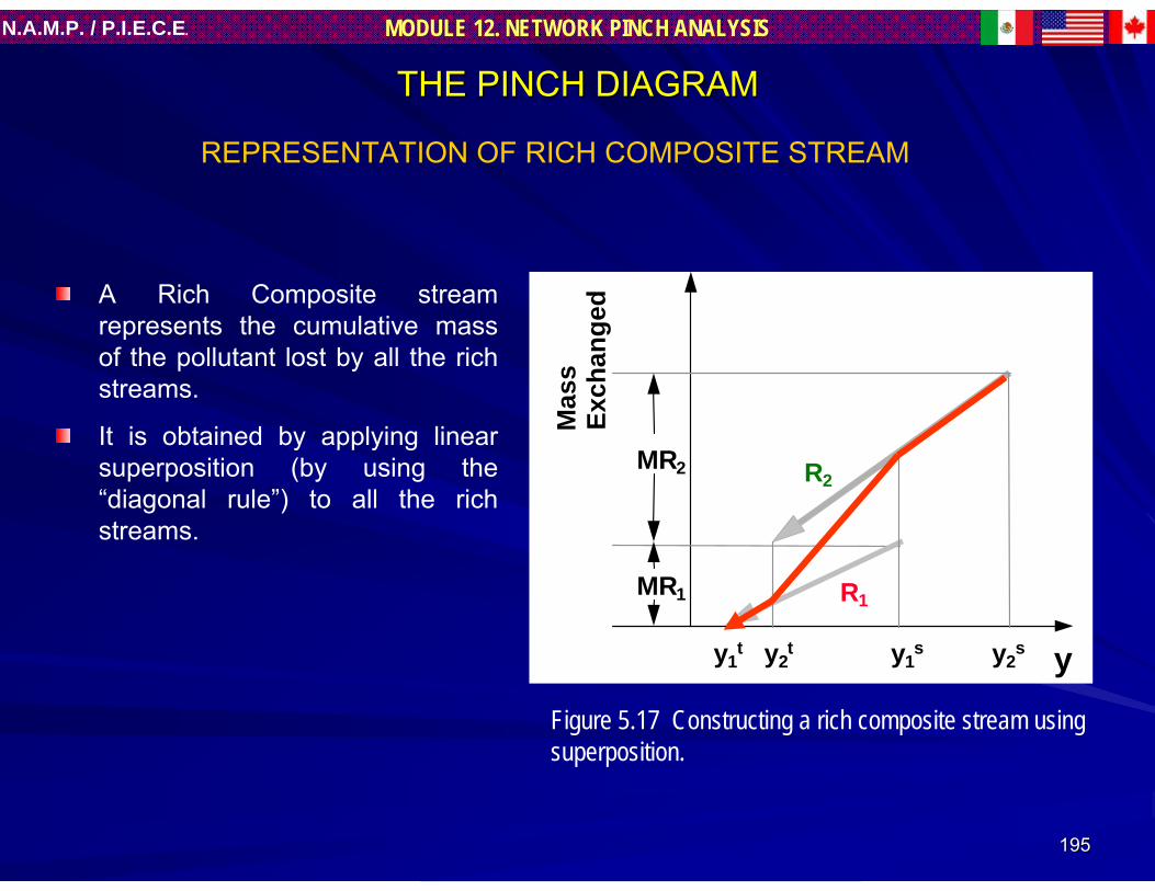
195195
MODULE 12. NETWORK PINCH ANALYSISN.A.M.P. / P.I.E.C.E.
A Rich Composite stream represents the cumulative mass of the pollutant lost by all the rich streams.
It is obtained by applying linear superposition (by using the “diagonal rule”) to all the rich streams.
THE PINCH DIAGRAMTHE PINCH DIAGRAM
REPRESENTATION OF RICH COMPOSITE STREAM
MR2
MR1 R1
R2
y1t y2
t y1s y2
s y
Mas
s Ex
chan
ged
Figure 5.17 Constructing a rich composite stream usingsuperposition.

196196
MODULE 12. NETWORK PINCH ANALYSISN.A.M.P. / P.I.E.C.E.
We establish NSP lean composition scales (one for each process MSA) that are in one-one correspondence with the rich scale.The mass of pollutant that can be gained by each process MSA is plotted vs the composition scale of that MSA.Each process MSA is represented as an arrow extending between supply and target composition.The Mass of pollutant that can be gained by the jth process MSA is
MSj = Lcj(xt
j -xsj) j = 1, 2, …, NSP
The vertical scale is only relative and any stream can be moved up or down on the diagram.
THE PINCH DIAGRAMTHE PINCH DIAGRAM
INDIVIDUAL REPRESENTATION FOR LEAN STREAMS
MS 2
MS 1
S2
S1
x1s
x2s
x1t
x2t
y
Mass Exchanged
xy b
m11
1
1=
−− ε
xy b
m22
2
2=
−− ε
Figure 5.18 Representation mass exchanged by two process MSAs.
(5.33)

197197
MODULE 12. NETWORK PINCH ANALYSISN.A.M.P. / P.I.E.C.E.
A convenient way of vertically placing each arrow is to stack the process MSAs on top of one another starting with the MSA having the lowest supply composition.
A lean composite stream representing the cumulative mass of the pollutant gained by all the MSAs is obtained by using the diagonal rule for superposition.
THE PINCH DIAGRAMTHE PINCH DIAGRAM
REPRESENTATION OF RICH COMPOSITE STREAM
MS 2
MS 1
S2
S1
x1s
x2s
x1t
x2t
y
Mass Exchanged
xy b
m11
1
1=
−− ε
xy b
m22
2
2=
−− ε
Figure 5.19 Constructing a lean composite stream usingsuperposition.

198198
MODULE 12. NETWORK PINCH ANALYSISN.A.M.P. / P.I.E.C.E.
Both composite streams are plotted on the same diagram.
The lean composite stream can be slid down until touches the waste composite stream
The point where the two composite streams touch is called the “mass-exchange pinch point”: hence the name “pinch diagram”.
THE PINCH DIAGRAMTHE PINCH DIAGRAM
CONSTRUCTING THE PINCH DIAGRAM
Lean CompositeStream
Rich CompositeStream
yx1
x2
Integratedmass Exchanged
Excess capacityof Process MSAs
Load to beRemoved byExternalMSAs
Mas
s E
xcha
nged
Mass ExchangePinch Point
Figure 5.20 The mass-exchange pinch diagram.

199199
MODULE 12. NETWORK PINCH ANALYSISN.A.M.P. / P.I.E.C.E.
INTEGRATED MASS EXCHANGE.INTEGRATED MASS EXCHANGE.The vertical overlap between the two composite streams representThe vertical overlap between the two composite streams represents the maximum s the maximum amount of the pollutant that can be transferred from the waste samount of the pollutant that can be transferred from the waste streams to the treams to the process process MSAsMSAs..
EXCESS CAPACITY OF PROCESS EXCESS CAPACITY OF PROCESS MSAsMSAs..It corresponds to the capacity of the process It corresponds to the capacity of the process MSAsMSAs to remove pollutants that cannot to remove pollutants that cannot be used because of thermodynamic unfeasibility.be used because of thermodynamic unfeasibility.According to the designerAccording to the designer’’s preference or to the specific circumstances of the s preference or to the specific circumstances of the process such excess can be eliminated from service by lowering tprocess such excess can be eliminated from service by lowering the he flowrateflowrate and/or and/or the outlet composition of one or more of the process the outlet composition of one or more of the process MSAsMSAs..
LOAD TO BE REMOVED BY EXTERNAL LOAD TO BE REMOVED BY EXTERNAL MSAsMSAs..It is the vertical distance of the waste composite stream which It is the vertical distance of the waste composite stream which lies below the lower lies below the lower end of the lean composite stream.end of the lean composite stream.
THE PINCH DIAGRAMTHE PINCH DIAGRAM
INTERPRETING THE PINCH DIAGRAM
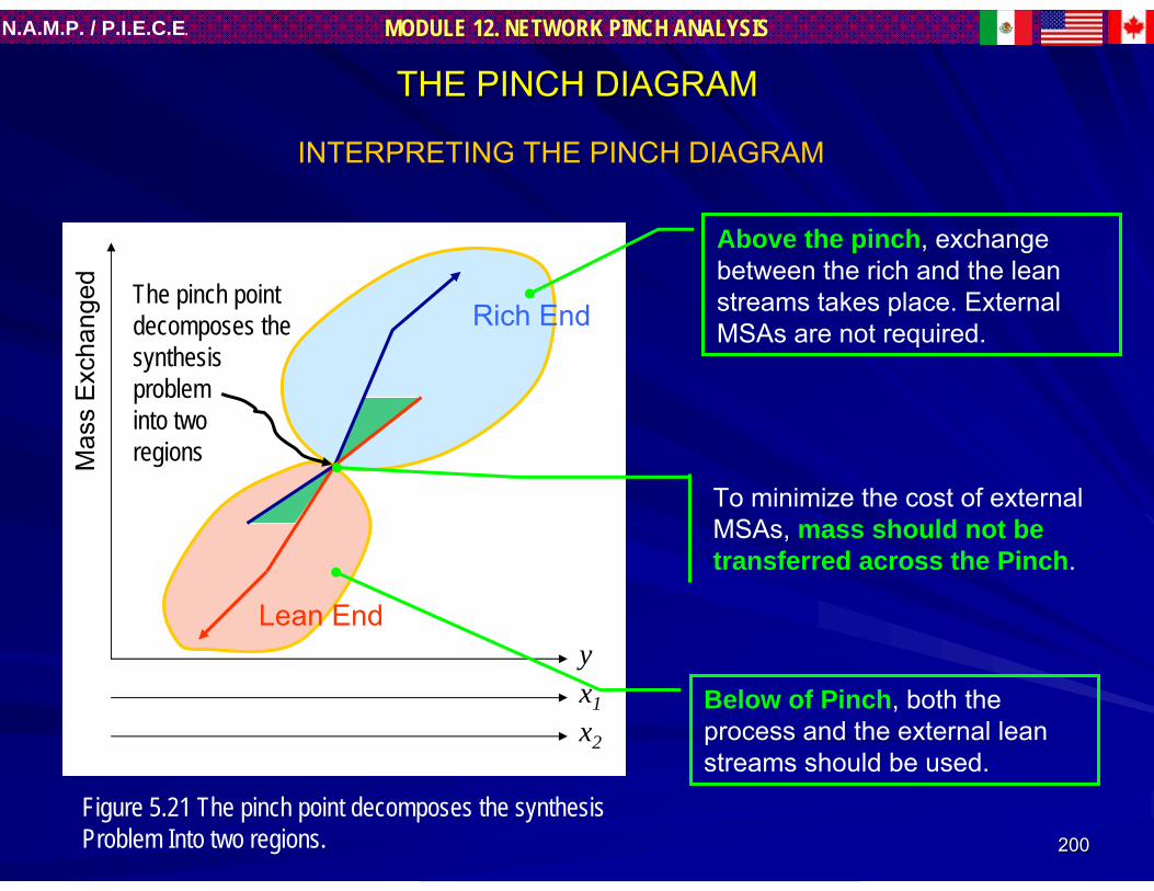
200200
MODULE 12. NETWORK PINCH ANALYSISN.A.M.P. / P.I.E.C.E.
THE PINCH DIAGRAMTHE PINCH DIAGRAM
INTERPRETING THE PINCH DIAGRAM
yx1
x2
Mas
s E
xcha
nged The pinch point
decomposes thesynthesisprobleminto tworegions.
Rich End
Lean End
Above the pinch, exchange between the rich and the lean streams takes place. External MSAs are not required.
Below of Pinch, both the process and the external lean streams should be used.
To minimize the cost of external MSAs, mass should not be transferred across the Pinch.
Figure 5.21 The pinch point decomposes the synthesisProblem Into two regions.

201201
MODULE 12. NETWORK PINCH ANALYSISN.A.M.P. / P.I.E.C.E.
5.2.2 GRAPHICAL APPROACH: MASS EXCHANGE 5.2.2 GRAPHICAL APPROACH: MASS EXCHANGE DIAGRAMDIAGRAM
EXAMPLE 1:EXAMPLE 1:
RECOVERY OF BENZENE FROM GASEOUS EMISSION OF A RECOVERY OF BENZENE FROM GASEOUS EMISSION OF A POLYMER PRODUCTION PROCESS.POLYMER PRODUCTION PROCESS.

202202
MODULE 12. NETWORK PINCH ANALYSISN.A.M.P. / P.I.E.C.E.
EXAMPLE 1:EXAMPLE 1:RECOVERY OF BENZENE FROM GASEOUS EMISSION OF A RECOVERY OF BENZENE FROM GASEOUS EMISSION OF A
POLYMER PRODUCTION PROCESSPOLYMER PRODUCTION PROCESS..
PROCESS DESCRIPTION.The copolymer is produced via two-stage reaction. The monomer are first dissolved in a
benzene-based solvent. The mixed-monomer mixture is fed to the first stage of reaction where a catalytic solution is added. Several additives (extending oil, inhibitors, and special additives) are mixed in a mechanically stirred column. The resulting solution is fed to the second-stage reactor, where the copolymer properties are adjusted. The stream leaving the second-stage reactor is passed to a separation system which produces four fraction: copolymer, unreacted monomers, benzene, and gaseous waste. The copolymer is fed to a coagulation and finishing section.
The unreacted monomers are recycled to the first-stage reactor, and the recovered benzene is returned to the monomer-mixing tank.
Figure 5.22 shows a simplified flowsheet of a copolymerization plant.
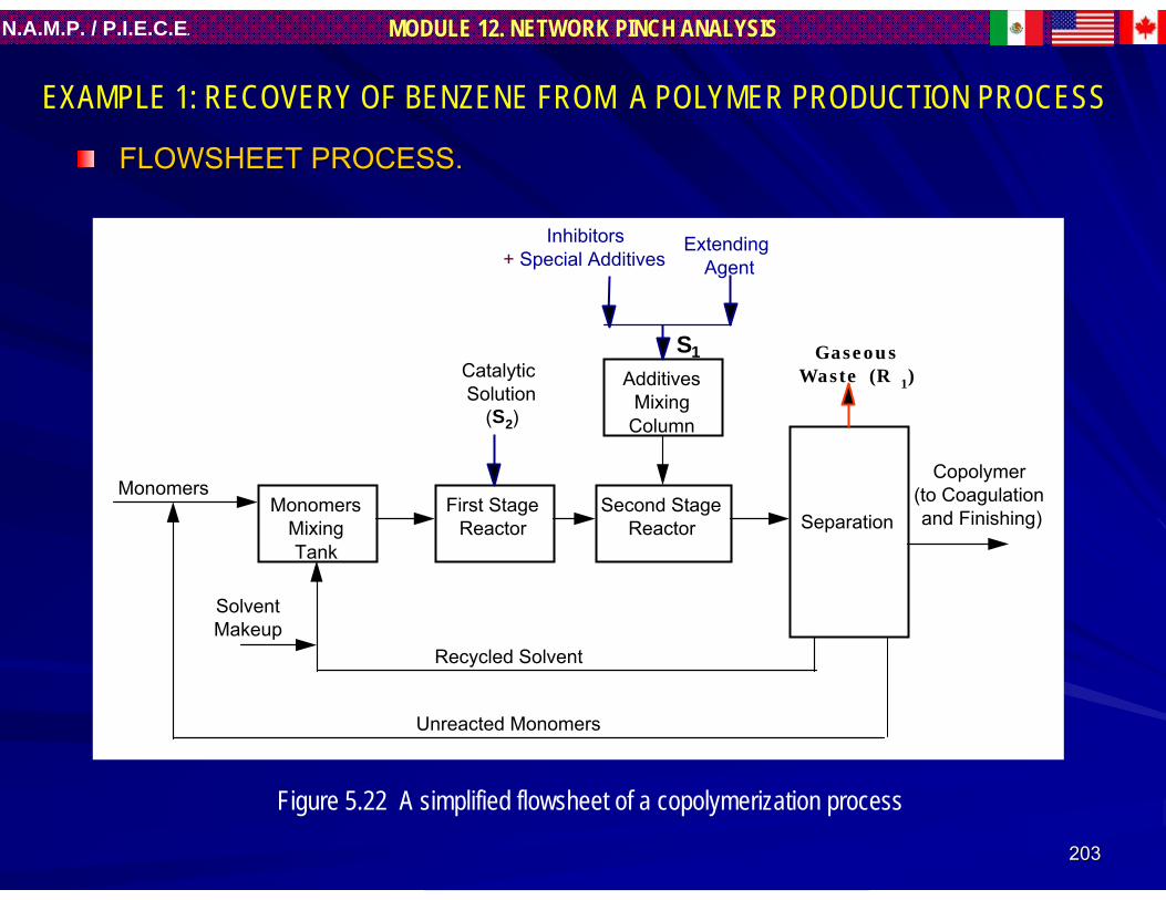
203203
MODULE 12. NETWORK PINCH ANALYSISN.A.M.P. / P.I.E.C.E.
Monomers
SolventMakeup
First StageReactor
Second StageReactor Separation
Copolymer (to Coagulation and Finishing)
Catalytic Solution
(S2)
Extending Agent
Recycled Solvent
Unreacted Monomers
GaseousWaste (R 1)
MonomersMixingTank
AdditivesMixing
Column
Inhibitors+ Special Additives
S1
Figure 5.22 A simplified flowsheet of a copolymerization process
FLOWSHEET PROCESS.FLOWSHEET PROCESS.
EXAMPLE 1: RECOVERY OF BENZENE FROM A POLYMER PRODUCTION PROCESS

204204
MODULE 12. NETWORK PINCH ANALYSISN.A.M.P. / P.I.E.C.E.
RICH STREAMRICH STREAMThe gaseous waste is the rich stream, R1, contains benzene as the primary pollutant
that should be recovered.
LEAN STREAMS. MASS SEPARATION AGENTS (MSA).LEAN STREAMS. MASS SEPARATION AGENTS (MSA).Process Process MSAsMSAs: : two process MSAs are considered for recovering benzene from the
gaseous waste. They are the additives, S1, and the liquid catalytic solution, S2. The use of these process MSAs offers several advantages:
– They can be used at virtually no operating cost.– Its positive environmental impact.– Economic incentive since it reduces the benzene makeup needed to
compensate for the processing losses.– The additives mixing column can be used as an absorption column by bubbling
the gaseous waste into the additives.
EXAMPLE 1: RECOVERY OF BENZENE FROM A POLYMER PRODUCTION PROCESS
Stream Description FlowrateGI, kgmol/s
Supply composition(mole fraction), ys
i
Target composition(mole fraction), yt
i
R1
Off-gas fromproduct
separation0.2 0.0020 0.0001
Table 5.1 Data waste stream for the benzene removal example.

205205
MODULE 12. NETWORK PINCH ANALYSISN.A.M.P. / P.I.E.C.E.
The equilibrium data for benzene in the two process MSAs are given by:
y = 0.25 x1 (5.34) and y = 0.50 x2 (5.35)where y, x1 and x2 are the mole fractions of benzene in the gaseous waste, S1 and S2
respectively.
The minimum allowable composition difference (ε) for S1 and S2 should not be less than 0.001.
EXAMPLE 1: RECOVERY OF BENZENE FROM A POLYMER PRODUCTION PROCESS
Stream DescriptionUpper boundon flowrateLC
j kg mol/s
Supply compositionof benzene
(mole fraction), xsj
Target compositionof benzene
(mole fraction), xtj
S1 Additives 0.08 0.003 0.006S2 Catalytic solution 0.05 0.002 0.004
Table 5.2 Data of process lean stream for the benzene removal example.
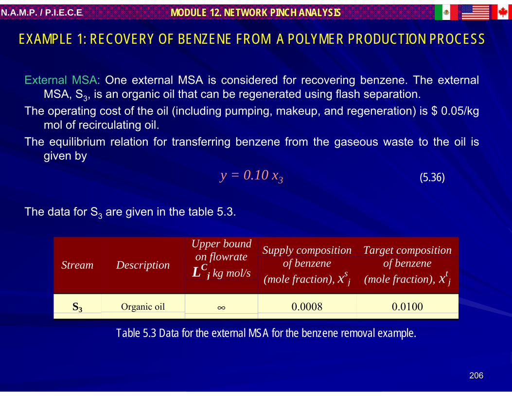
206206
MODULE 12. NETWORK PINCH ANALYSISN.A.M.P. / P.I.E.C.E.
External MSA: One external MSA is considered for recovering benzene. The external MSA, S3, is an organic oil that can be regenerated using flash separation.
The operating cost of the oil (including pumping, makeup, and regeneration) is $ 0.05/kg mol of recirculating oil.
The equilibrium relation for transferring benzene from the gaseous waste to the oil is given by
y = 0.10 x3
The data for S3 are given in the table 5.3.
EXAMPLE 1: RECOVERY OF BENZENE FROM A POLYMER PRODUCTION PROCESS
Stream Description
Upper boundon flowrateLC
j kg mol/s
Supply compositionof benzene
(mole fraction), xsj
Target compositionof benzene
(mole fraction), xtj
S3 Organic oil ∞ 0.0008 0.0100
(5.36)
Table 5.3 Data for the external MSA for the benzene removal example.

207207
MODULE 12. NETWORK PINCH ANALYSISN.A.M.P. / P.I.E.C.E.
DESIGN TASK.DESIGN TASK.Using the graphical pinch approach, synthesize a cost-effective Mass exchanger
Network that can be used to remove benzene from the gaseous waste, Fig. 5.22
EXAMPLE 1: RECOVERY OF BENZENE FROM A POLYMER PRODUCTION PROCESS
Monomers
SolventMakeup
First StageReactor
Second StageReactor Separation
Copolymer (to Coagulation and Finishing)
Catalytic Solution
Additives (Extending Agent, Inhibitors
and Special Additives)
Recycled Solvent
Unreacted Monomers
GaseousWaste
Mixing
OilS3
Regeneration
OilMakeup
Benzene Recovery MEN R1
S1S2
ToAtmos-phere
Benzene
Figure 5.22 The copolymerization process with a benzene recovery MEN.

208208
MODULE 12. NETWORK PINCH ANALYSISN.A.M.P. / P.I.E.C.E.
SOLUTION.SOLUTION. CONSTRUCTING THE PINCH DIAGRAMCONSTRUCTING THE PINCH DIAGRAM..Constructing the Rich Composite Stream.
EXAMPLE 1: RECOVERY OF BENZENE FROM A POLYMER PRODUCTION PROCESS
6.0
0.0001 0.0005 0.0010 0.0015 0.0020 0.0025 y0.0
2.0
1.0
3.0
4.0
5.0
Ma s
s Ex
c han
ged,
1 0-4
k mo l
eB
e nz e
n e/ s
Rich CompositeStream
0.0000
3.8
ys1
yt1
m = G1
Figure 5.23 Rich composite stream for the benzene recovery example.
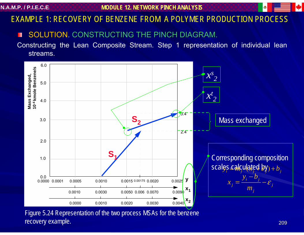
209209
MODULE 12. NETWORK PINCH ANALYSISN.A.M.P. / P.I.E.C.E.
SOLUTIONSOLUTION. . CONSTRUCTING THE PINCH DIAGRAM.CONSTRUCTING THE PINCH DIAGRAM.Constructing the Lean Composite Stream. Step 1 representation of individual lean
streams.
EXAMPLE 1: RECOVERY OF BENZENE FROM A POLYMER PRODUCTION PROCESS
0.0001 0.0005 0.0010 0.0015 0.0020 0.0025 y0.0
2.0
1.0
3.0
4.0
5.0
6.0
Mas
s Ex
chan
ged,
10-4
kmol
eB
enze
ne/s
0.0010 0.0030 0.0050 0.0070 0.0090x1
0.0000 0.0010 0.0020 0.0030 0.0040x2
0.0000
2.4
0.00175
0.006
3.4
S1
S2
xs2
xt2
Mass exchanged
Corresponding composition scales calculated by( )i j j j jy m x bε= ⋅ + +
i jj j
j
y bx
mε
−= −
Figure 5.24 Representation of the two process MSAs for the benzenerecovery example.
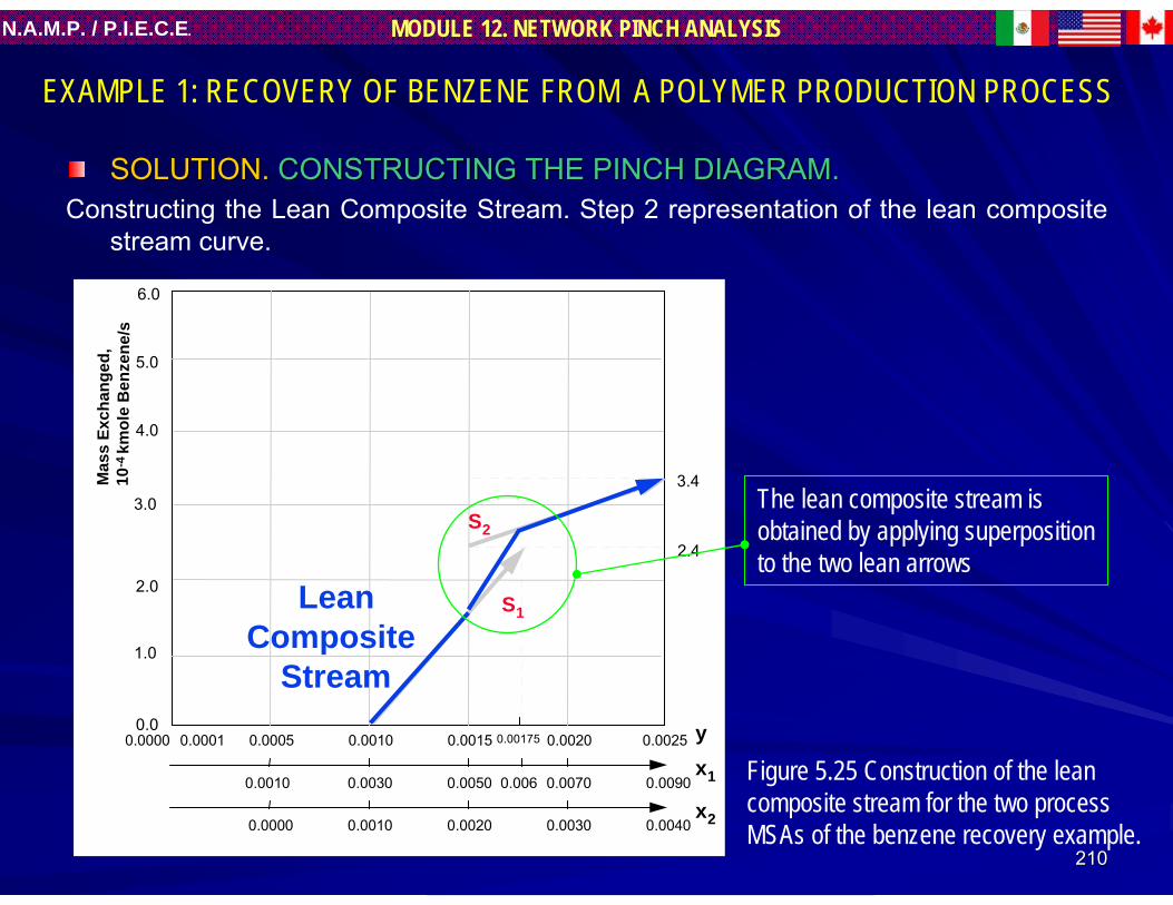
210210
MODULE 12. NETWORK PINCH ANALYSISN.A.M.P. / P.I.E.C.E.
SOLUTION.SOLUTION. CONSTRUCTING THE PINCH DIAGRAM.CONSTRUCTING THE PINCH DIAGRAM.Constructing the Lean Composite Stream. Step 2 representation of the lean composite
stream curve.
EXAMPLE 1: RECOVERY OF BENZENE FROM A POLYMER PRODUCTION PROCESS
0.0001 0.0005 0.0010 0.0015 0.0020 0.0025 y0.0
2.0
1.0
3.0
4.0
5.0
6.0
Ma s
s Ex
c han
g ed,
1 0-4
k mo l
eB
e nz e
n e/ s
0.0010 0.0030 0.0050 0.0070 0.0090x1
0.0000 0.0010 0.0020 0.0030 0.0040x2
0.0000
2.4
0.00175
0.006
3.4
S1
S2
LeanComposite
Stream
The lean composite stream isobtained by applying superpositionto the two lean arrows
Figure 5.25 Construction of the lean composite stream for the two process MSAs of the benzene recovery example.

211211
MODULE 12. NETWORK PINCH ANALYSISN.A.M.P. / P.I.E.C.E.
SOLUTION.SOLUTION. CONSTRUCTING THE PINCH DIAGRAMCONSTRUCTING THE PINCH DIAGRAM..The pinch diagram is constructed by combining the two composite curves. The lean composite curve stream is slid vertically until it is completely above the rich composite stream.
EXAMPLE 1: RECOVERY OF BENZENE FROM A POLYMER PRODUCTION PROCESS
Lean CompositeStream
0.0001 0.0005 0.0010 0.0015 0.0020 0.0025 y0.0
2.0
1.0
3.0
4.0
5.0
6.0
Mas
s Ex
chan
ged,
10-4
kmol
eB
enze
ne/s
0.0010 0.0030 0.0050 0.0070 0.0090x1
0.0000 0.0010 0.0020 0.0030 0.0040x2
Rich CompositeStream
0.0000
3.8
0.00175
0.006
1.8
4.2
5.2
PinchPoint
Figure 5.26 The pinch diagram for theBenzene Recovery example(εε11 = = εε22 =0.001).=0.001).

212212
MODULE 12. NETWORK PINCH ANALYSISN.A.M.P. / P.I.E.C.E.
SOLUTION.SOLUTION. INTERPRETING THE PINCH DIAGRAMINTERPRETING THE PINCH DIAGRAM..
EXAMPLE 1: RECOVERY OF BENZENE FROM A POLYMER PRODUCTION PROCESS
Lean CompositeStream
0.0001 0.0005 0.0010 0.0015 0.0020 0.0025 y0.0
2.0
1.0
3.0
4.0
5.0
6.0
Mas
s Ex
chan
ged,
10-4
kmol
eB
enze
ne/s
0.0010 0.0030 0.0050 0.0070 0.0090x1
0.0000 0.0010 0.0020 0.0030 0.0040x2
Rich CompositeStream
Excess Capacityof Process MSA’s
PinchPoint
0.0000
3.8
0.00175
0.006
1.8
4.2
5.2
Load to BeRemoved By
External MSA’s
IntegratedMass
ExchangePinch pint islocated at:(y, x1, x2) =(0.0010,0.0030,0.10010)
Excess capacityof process MSAsis 1.4x10⁻⁴ kg mol/s
1.8 x 10⁻⁴ kg mol/s
Figure 5.27 Interpreting the pinch diagram for the benzene recovery example.

213213
MODULE 12. NETWORK PINCH ANALYSISN.A.M.P. / P.I.E.C.E.
SOLUTION. INTERPRETING THE PINCH DIAGRAM..
REMOVING EXCESS CAPACITY. The excess capacity of the process MSAs is eliminated byavoiding the use of S2 and reducing the flowrate and/or outletcomposition of S1.
There are infinite combinations of L1 and x1out that can be
used to remove the excess capacity of S1 according to thefollowing material balance:
S1 = L1(x1out - x1
s)S1 is benzene load above the pinch to be removed.
2 x 10 -4 = L1 (x1out - 0.003)
Nonetheless, since the additives-mixing column will be used for absorption, the whole flowrate of S1 (0.08 kg/s) should be fed to the column. Hence according to Eq. (5.38), the outlet composition of S1 is 0.0055.
The same result can be obtained graphically as shown in Fig. 5.28.
EXAMPLE 1: RECOVERY OF BENZENE FROM A POLYMER PRODUCTION PROCESS
Excess capacity(5.37)
(5.38)
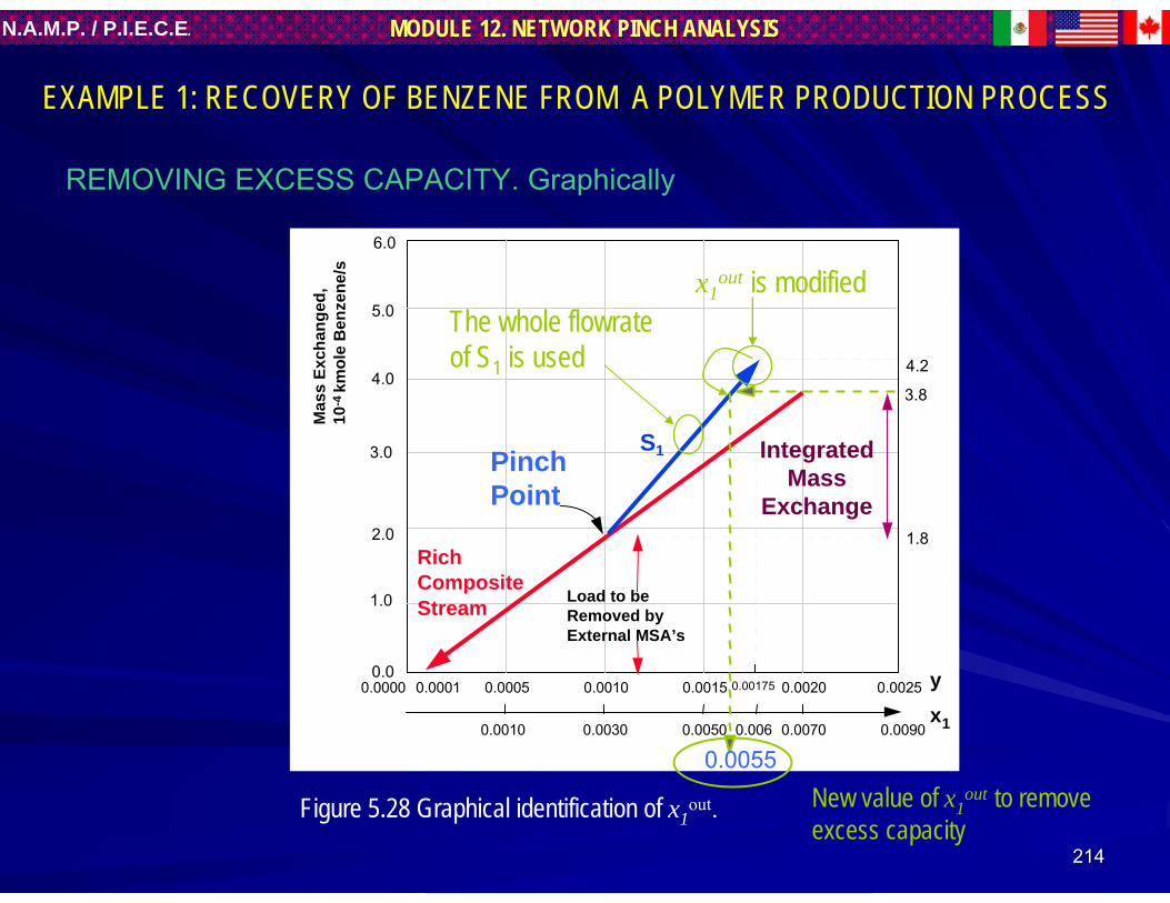
214214
MODULE 12. NETWORK PINCH ANALYSISN.A.M.P. / P.I.E.C.E.
EXAMPLE 1: RECOVERY OF BENZENE FROM A POLYMER PRODUCTION PROCESS
REMOVING EXCESS CAPACITY. Graphically
0.0001 0.0005 0.0010 0.0015 0.0020 0.0025 y0.0
2.0
1.0
3.0
4.0
5.0
6.0
Mas
s Ex
chan
ged,
10-4
kmol
eB
enze
ne/s
0.0010 0.0030 0.0050 0.0070 0.0090x1
Load to beRemoved byExternal MSA’s
Rich CompositeStream
PinchPoint
0.0000
3.8
0.00175
0.006
1.8
4.2
IntegratedMass
Exchange
0.0055
S1
The whole flowrateof S1 is used
x1out is modified
New value of x1out to remove
excess capacityFigure 5.28 Graphical identification of x1
out.

215215
MODULE 12. NETWORK PINCH ANALYSISN.A.M.P. / P.I.E.C.E.
SELECTION OF THE OPTIMAL VALUE OF SELECTION OF THE OPTIMAL VALUE OF εε..In this example it is desired to maximize the integrated mass exchanged above the
pinch. As can see on the pinch diagram when εε11 increases, the x1 axis moves to the right relative to the y axis and, consequently, the extend of integrated mass exchange decreased leading to a higher cost of external MSAs.
The increase of εε11 to 0.002 results in the following mass integration values:
Thus: the optimum εε11 in this example is the smallest permissible value given in the problem statement to be 0.001.
EXAMPLE 1: RECOVERY OF BENZENE FROM A POLYMER PRODUCTION PROCESS
ε1 = 0.001 ε1 = 0.002Load of benzene to be removedby external MSAs (kg mol/s) 1.8 x 10 -4 2.3 x 10 -4
Integrated mass exchanged 2.0 x 10 -4 1.5 x 10 -4
Excess capacity of processMSAs 1.4 x 10 -4 1.0 x 10 -4

216216
MODULE 12. NETWORK PINCH ANALYSISN.A.M.P. / P.I.E.C.E.
EXAMPLE 1: RECOVERY OF BENZENE FROM A POLYMER PRODUCTION PROCESSTHE PINCH DIAGRAM WHEN ε1 = 0.002
LeanComposite
Stream
0.0001 0.0005 0.0010 0.0015 0.0020 0.0025 y0.0
2.0
1.0
3.0
4.0
5.0
6.0
Ma s
s Ex
c han
ged,
1 0-4
k mo l
eB
e nz e
n e/ s
0.0000 0.0020 0.0040 0.0060 0.0080x1
0.0000 0.0010 0.0020 0.0030 0.0040x2
Rich CompositeStream
Excess Capacityof Process MSA’s
PinchPoint
0.0000
3.8
2.3
4.7
5.7
Load to BeRemoved By
External MSA’s
IntegratedMass
Exchange
0.0030
0.00125
Figure 5.29 The pinch diagram when ε1 is increased to 0.002.
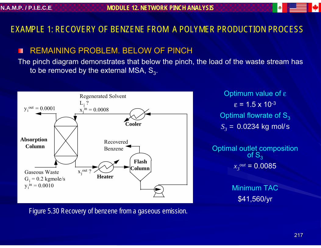
217217
MODULE 12. NETWORK PINCH ANALYSISN.A.M.P. / P.I.E.C.E.
EXAMPLE 1: RECOVERY OF BENZENE FROM A POLYMER PRODUCTION PROCESS
REMAINING PROBLEM. BELOW OF PINCHREMAINING PROBLEM. BELOW OF PINCHThe pinch diagram demonstrates that below the pinch, the load of the waste stream has
to be removed by the external MSA, S3.
RecoveredBenzene
FlashColumn
yiout = 0.0001
Gaseous WasteGi = 0.2 kgmole/syi
in = 0.0010
xjout ?
Heater
Cooler
Regenerated SolventLj ?xj
in = 0.0008
AbsorptionColumn
Optimum value of εε = 1.5 x 10⁻³
Optimal flowrate of S3
S3 = 0.0234 kg mol/s
Optimal outlet composition of S3
x3out = 0.0085
Minimum TAC$41,560/yr
Figure 5.30 Recovery of benzene from a gaseous emission.
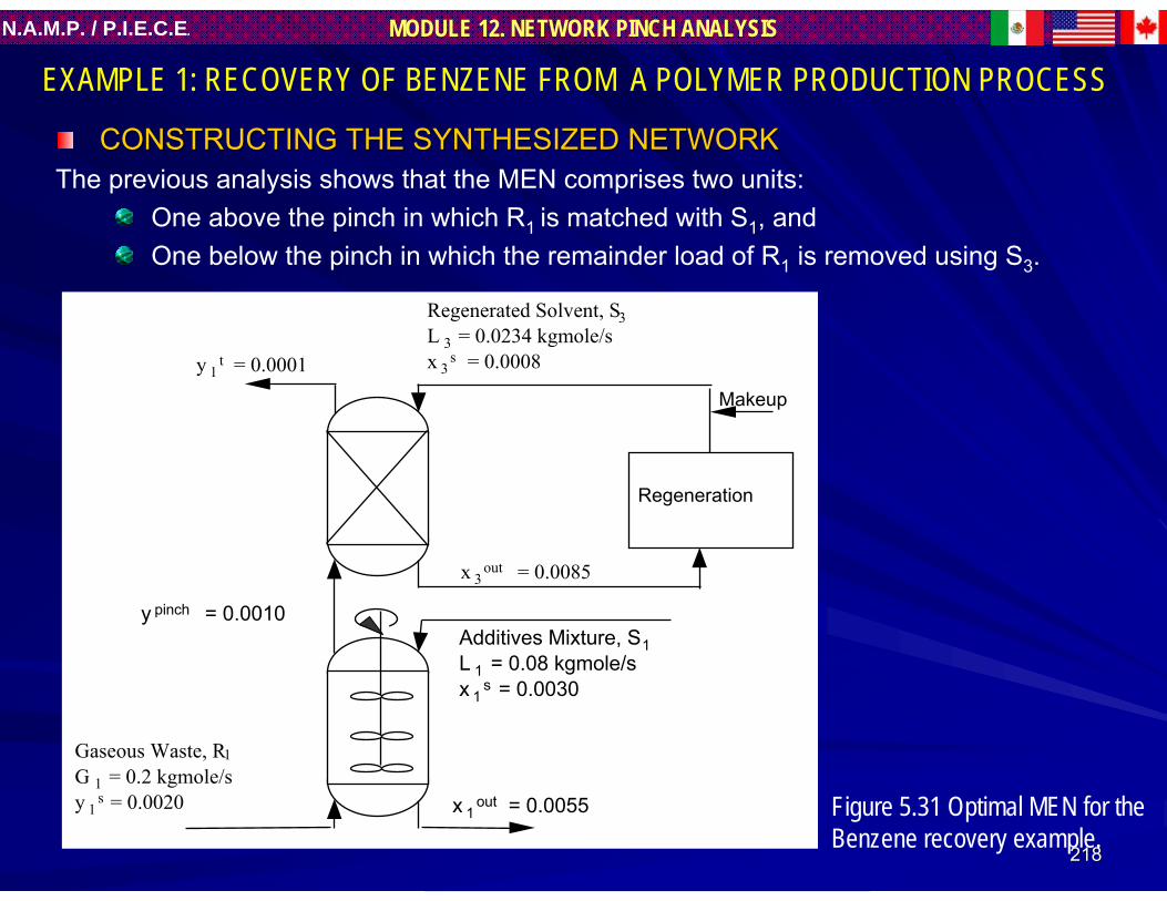
218218
MODULE 12. NETWORK PINCH ANALYSISN.A.M.P. / P.I.E.C.E.
EXAMPLE 1: RECOVERY OF BENZENE FROM A POLYMER PRODUCTION PROCESS
CONSTRUCTING THE SYNTHESIZED NETWORKCONSTRUCTING THE SYNTHESIZED NETWORKThe previous analysis shows that the MEN comprises two units:
One above the pinch in which R1 is matched with S1, andOne below the pinch in which the remainder load of R1 is removed using S3.
y 1t = 0.0001
Gaseous Waste, R1G 1 = 0.2 kgmole/sy 1
s = 0.0020
x 3out = 0.0085
Regenerated Solvent, S3L 3 = 0.0234 kgmole/sx 3
s = 0.0008
Regeneration
Makeup
y pinch = 0.0010Additives Mixture, S1L 1 = 0.08 kgmole/sx 1
s = 0.0030
x 1out = 0.0055 Figure 5.31 Optimal MEN for the
Benzene recovery example.

219219
MODULE 12. NETWORK PINCH ANALYSISN.A.M.P. / P.I.E.C.E.
5.2 SYNTHESIS of MASS EXCHANGE 5.2 SYNTHESIS of MASS EXCHANGE NETWORKSNETWORKS
5.2.1 Problem statement.5.2.1 Problem statement.
5.2.2 Graphical approach: Mass Exchange 5.2.2 Graphical approach: Mass Exchange Diagram.Diagram.
5.2.3 Algebraic approach: Composition 5.2.3 Algebraic approach: Composition Interval DiagramInterval Diagram..
5.2.4 Design for Minimum Number of Mass 5.2.4 Design for Minimum Number of Mass Exchanger Units.Exchanger Units.

220220
MODULE 12. NETWORK PINCH ANALYSISN.A.M.P. / P.I.E.C.E.
5.2.3 Algebraic Approach: Composition Interval 5.2.3 Algebraic Approach: Composition Interval DiagramDiagram
Notwithstanding the usefulness of the pinch diagram, it is subject to the
accuracy problems associated with any graphical approach. This is
particularly true when there is a wide range of operating compositions for
the waste and the lean streams. In such cases, an algebraic method is
recommended.
This section presents an algebraic procedure which yields results that are
equivalent to those provided by the graphical pinch analysis.
The algebraic method can be programmed and formulated as optimization
problems.
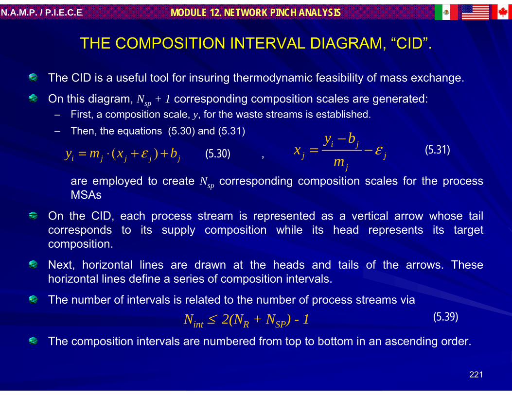
221221
MODULE 12. NETWORK PINCH ANALYSISN.A.M.P. / P.I.E.C.E.
THE COMPOSITION INTERVAL DIAGRAM, THE COMPOSITION INTERVAL DIAGRAM, ““CIDCID””..
The CID is a useful tool for insuring thermodynamic feasibility of mass exchange.
On this diagram, Nsp + 1 corresponding composition scales are generated:– First, a composition scale, y, for the waste streams is established.– Then, the equations (5.30) and (5.31)
are employed to create Nsp corresponding composition scales for the process MSAs
On the CID, each process stream is represented as a vertical arrow whose tail corresponds to its supply composition while its head represents its target composition.
Next, horizontal lines are drawn at the heads and tails of the arrows. These horizontal lines define a series of composition intervals.
The number of intervals is related to the number of process streams via
Nint ≤ 2(NR + NSP) - 1The composition intervals are numbered from top to bottom in an ascending order.
( )i j j j jy m x bε= ⋅ + +i j
j jj
y bx
mε
−= −,(5.30) (5.31)
(5.39)
222222
MODULE 12. NETWORK PINCH ANALYSISN.A.M.P. / P.I.E.C.E.
The index k will be used to designate an interval with k = 1 being the uppermost interval and k = Nint being the lowermost interval.
Figure 5.31 provides a schematic representation of the CID.
Within any interval. It is thermodynamically feasible to transfer mass from a waste stream in an interval k to any MSA which lies an interval k* below it (i.e., k* ≥ k).

223223
MODULE 12. NETWORK PINCH ANALYSISN.A.M.P. / P.I.E.C.E.
Interval
RichStreams
Process MSA’sx y b m1 1 1 1= − −( ) / ε x y b m2 2 2 2= − −( ) / ε x y b mNsp Nsp Nsp Nsp= − −( ) / ε
1
2
3
4
5
6
7
8
9
10
.
.
.Nint
y1s R1
y1t
y2s
yNRs
y2t
yNRt
R2
RNR
x1t
x1s
S1
S2
x2t
x2s
xNspt
xNsps
SNsp
Figure 5.31 The composition interval diagram “CID”.

224224
MODULE 12. NETWORK PINCH ANALYSISN.A.M.P. / P.I.E.C.E.
TABLE OF EXCHANGEABLE LOADS, TABLE OF EXCHANGEABLE LOADS, ““TELTEL””..
The objective of constructing a TEL is to determine the mass exchange loads of the process streams in each composition interval.
The exchangeable load of the ith waste stream which passes through the kthinterval is defined as
WRj,k = Gi(yk-1 - yk)
where yk-1 and yk are the waste-scale composition of the transferrable species which respectively correspond to the top and the bottom lines defining the kth interval.
The exchangeable load of the jth process MSA which passes through the kthinterval is computed through the following expression
WSj,k = LC
j (xj,k-1 - xj,k)
where xj,k-1 and xj,k are the composition on the jth lean composition scale which respectively correspond to the higher and lower horizontal lines bounding the kthinterval.
(5.40)
(5.41)

225225
MODULE 12. NETWORK PINCH ANALYSISN.A.M.P. / P.I.E.C.E.
Clearly, if a stream does not pass through an interval, its load within that interval is zero.
The collective load of the waste streams within the kth interval is calculated by summing up the individual loads of the waste streams that pass through that interval, I.e.
The collective load of the lean streams within the kth interval is evaluated as follow:
, passes through interval
R Rk i k
i kW W= ∑
, passes through interval
S Sk j k
j kW W= ∑
(5.42)
(5.43)

226226
MODULE 12. NETWORK PINCH ANALYSISN.A.M.P. / P.I.E.C.E.
MASS EXCHANGE CASCADE DIAGRAMMASS EXCHANGE CASCADE DIAGRAM
We are now in a position to incorporate material balance into the synthesis procedure with the objective of allocating the pinch point as well as evaluating excess capacity of process MSAs and load to be removed by external MSAs.These aspect are assessed through the mass-exchange cascade diagram.
For the kth composition interval, one can write the following component material balance for the key pollutant:
where δk-1 and δk are the residual masses of the key pollutant entering and leaving the kth interval.
Equation (5.44) indicates that the total mass input of the key component to the kthinterval is due to collective load of the waste stream in that interval as well as the residual mass of the key component leaving the interval above it, δk-1.
1R S
k k k kW Wδ δ−+ − = (5.44)

227227
MODULE 12. NETWORK PINCH ANALYSISN.A.M.P. / P.I.E.C.E.
A total mass, WSk, of the key pollutant is transferred to the MSAs in the kth interval.
Hence, a residual mass, δk, of the pollutant leaving the kth interval can be calculated via Eq.( ). This output residual also constitutes the influent residual to the subsequent interval.
Fig. 5.31 illustrates the component material balance for the key pollutant around the kth composition interval.
kWkR Wk
S
δ k-1
δ k
Mass Recoveredfrom Rich
Streams
Mass Transferredto MSA’s
Residual Mass fromPreceeding Interval
Residual Mass toSubsequent Interval
Figure 5.31 A pollutant material balance around a composition interval

228228
MODULE 12. NETWORK PINCH ANALYSISN.A.M.P. / P.I.E.C.E.
δ0 = 0, It is worth pointing out that δ0 is zero since no waste streams exist above the first interval.
δk > 0, When all the δk’s are nonnegative Thermodynamic feasibility is insured.
δk < 0, A negative δk indicates that the capacity of the process lean streams at thatlevel is greater than the load of the waste streams. The most negative δkcorresponds to the excess capacity of the process MSAs in removing the pollutant. Therefore, this excess capacity of process MSAs should be reduced by lowering the flowrate and/or the outlet composition of one or more of the MSAs.
After removing the excess capacity of MSAs, one can construct a revised TEL in which the flowrates and/or outlet compositions of the process MSAs have been adjusted.
On the revised cascade diagram the location at which the residual mass is zero corresponds to the mass-exchange pinch composition. As expected, this location is the same as that with the most negative residual on the original cascade diagram.
Since an overall material balance for the network must be realized, the residual mass leaving the lowest composition interval of the revised cascade diagram must be removed by external MSAs.

229229
MODULE 12. NETWORK PINCH ANALYSISN.A.M.P. / P.I.E.C.E.
Summarizing the Synthesis of Summarizing the Synthesis of MENsMENs: Algebraic : Algebraic ApproachApproach..
Statementproblem
Create theCID
Generate the TEL
Construct the Revised TEL
- The excess capacity of process MSAs is themost negative residual mass
- Adjust the excess capacity by reducing theflowrates and/or outlet compositions of the process MSAs.
- The mass-exchange pinch is located wherethe residual mass leaving is cero.
- The residual mass leaving the bottom intervalis the amount of pollutant to be removed by external MSAs.

230230
MODULE 12. NETWORK PINCH ANALYSISN.A.M.P. / P.I.E.C.E.
Synthesis of mass exchange networks: algebraic approach.Synthesis of mass exchange networks: algebraic approach.EXAMPLE ON DEPHENOLIZATION OF AQUEOUS WASTESEXAMPLE ON DEPHENOLIZATION OF AQUEOUS WASTES
PROCESS DESCRIPTIONPROCESS DESCRIPTIONIn this process, two types of waste oil are handle: gas oil and lube oil. The two streams
are first dashed and demetallized. Next, atmospheric distillation is used to obtain light gases, gas oil, and a heavy product. The heavy product is distilled under vacuum to yield lube oil. Both the gas oil and the lube oil should be further processed to attain desired properties. The gas oil is steam stripped to remove light and sulfur impurities, then hydro treated. The lube oil is dewaxed / deasphaltedusing solvent extraction followed by steam stripping.
The process has two main sources of waste water. These are the condensate streams from the steam stripper. The principal pollutant in both wastewater streams is phenol. Phenol is of concern primarily because of its toxicity, oxygen depletion, and turbidity. In addition, phenol can cause objectionable taste and odor in fish flesh and potable water.

231231
MODULE 12. NETWORK PINCH ANALYSISN.A.M.P. / P.I.E.C.E.
PROCESS FLOWSHEET.PROCESS FLOWSHEET.
Synthesis of mass exchange networks: algebraic approach.Synthesis of mass exchange networks: algebraic approach.EXAMPLE ON DEPHENOLIZATION OF AQUEOUS WASTESEXAMPLE ON DEPHENOLIZATION OF AQUEOUS WASTES
Deashing andDemetallization
Gas Oil
MassExchangeNetwork
To finalfinishing
S1 S2 S3 S4 S5
To regen-eration &recycle
To phenolcondens-ation
R1
R2
R1
R2
S1
Atmospheric
DistillationStripping
Gas Oil
Steam
Stripping
Steam
Deashing andDemetallization
VacuumDistillat-ion
Dewaxing andDeasph-alting
Lube Oil
Air S5
Ion Exchange Resin S4
ActivatedCarbon S3
Lube Oil S2
WasteLube Oil
WasteGas Oil
Light Gases
Figure 5.32 Schematic representation of an oil recycling plant.

232232
MODULE 12. NETWORK PINCH ANALYSISN.A.M.P. / P.I.E.C.E.
RICH STREAM DATA.RICH STREAM DATA.
CANDIDATE CANDIDATE MSAsMSAs..–– 2 Process 2 Process MSAsMSAs::
Solvent extraction using gas oil (SSolvent extraction using gas oil (S11))Solvent extraction using lube oil (SSolvent extraction using lube oil (S22).).
–– 3 external 3 external MSAsMSAs::Adsorption using activated carbon (SAdsorption using activated carbon (S33))Ion exchange using polymeric resin (SIon exchange using polymeric resin (S44))Stripping using air (SStripping using air (S55))
Synthesis of mass exchange networks: algebraic approach.Synthesis of mass exchange networks: algebraic approach.EXAMPLE ON DEPHENOLIZATION OF AQUEOUS WASTESEXAMPLE ON DEPHENOLIZATION OF AQUEOUS WASTES
Stream Description FlowrateGI, kg/s
Supplycomposition,
ysi
Targetcomposition,
yti
R1Condensate from
first stripper 2 0.050 0.010
R2Condensate fromsecond stripper 1 0.030 0.006
Table 5.4 Data of waste stream for the dephenolization example.

233233
MODULE 12. NETWORK PINCH ANALYSISN.A.M.P. / P.I.E.C.E.
Synthesis of mass exchange networks: algebraic approach.Synthesis of mass exchange networks: algebraic approach.EXAMPLE ON DEPHENOLIZATION OF AQUEOUS WASTESEXAMPLE ON DEPHENOLIZATION OF AQUEOUS WASTES
PROCESS MSAs DATA
EQUILIBRIUM DATAGeneral equation for transferring phenol to the jth lean stream.
m1 = 2.00, m2 = 1.53, m3 = 0.02, m4 = 0.09 and m5 = 0.04
Stream DescriptionUpper boundon flowrate
Lcj, kg/s
Supplycomposition,
xsj
Targetcomposition,
xtj
S1 Gas oil 5 0.005 0.015
S2 Lube oil 3 0.010 0.030
Table 5.5 Data of process MSAs for the Dephenolization example.
jj xmy ⋅= (5.45)

234234
MODULE 12. NETWORK PINCH ANALYSISN.A.M.P. / P.I.E.C.E.
Synthesis of mass exchange networks: algebraic approach.Synthesis of mass exchange networks: algebraic approach.EXAMPLE ON DEPHENOLIZATION OF AQUEOUS WASTESEXAMPLE ON DEPHENOLIZATION OF AQUEOUS WASTES
MINIMUM ALLOWABLE COMPOSITION DIFFERENCEMINIMUM ALLOWABLE COMPOSITION DIFFERENCE
kgMSAphenol kg001.0=jε j = 1, 2, 3, 4, 5 (5.46)

235235
MODULE 12. NETWORK PINCH ANALYSISN.A.M.P. / P.I.E.C.E.
11 COMPOSITION INTERVAL DIAGRAM (CID).COMPOSITION INTERVAL DIAGRAM (CID).
Synthesis of mass exchange networks: algebraic approach.Synthesis of mass exchange networks: algebraic approach.EXAMPLE ON DEPHENOLIZATION OF AQUEOUS WASTESEXAMPLE ON DEPHENOLIZATION OF AQUEOUS WASTES
S O L U T I O NS O L U T I O N
IntervalRich Streams Process MSA’s
R1
R2
S2
S1
1
2
3
4
5
6
7
0.0500
0.0474
0.0320
0.0300
0.0168
0.0120
0.0100
0.0060
y0.0240
0.0227
0.0150
0.0140
0.0074
0.0050
0.0040
0.0020
0.0317
0.0300
0.0199
0.0186
0.0100
0.0068
0.0055
0.0029
x1 x2
Figure 5.33 The CID for the dephenolization example.

236236
MODULE 12. NETWORK PINCH ANALYSISN.A.M.P. / P.I.E.C.E.
22 TABLE OF EXCHANGEABLE LOADS (TEL).TABLE OF EXCHANGEABLE LOADS (TEL).
Synthesis of mass exchange networks: algebraic approach.Synthesis of mass exchange networks: algebraic approach.EXAMPLE ON DEPHENOLIZATION OF AQUEOUS WASTESEXAMPLE ON DEPHENOLIZATION OF AQUEOUS WASTES
S O L U T I O NS O L U T I O N
IntervalLoad of Waste Streams
kg phenol/sLoad of Process MSA’s
kg phenol/s
R1R2 R1 + R2
S2S1 S1 + S2
1
2
3
4
5
6
7
0.0052 - 0.0052 - - -
0.0308 - 0.0308 - 0.0303 0.0303
0.0040 - 0.0040 0.0050 0.0039 0.0089
0.0264 0.0132 0.0396 0.0330 0.0258 0.0588
0.0096 0.0048 0.0144 0.0120 - 0.0120
0.0040 0.0020 0.0060 - - -
- 0.0040 0.0040 - - -
Table 5.6 The TEL for the dephenolization example.

237237
MODULE 12. NETWORK PINCH ANALYSISN.A.M.P. / P.I.E.C.E.
3 MASS3 MASS--EXCHANGE CASCADE DIAGRAMEXCHANGE CASCADE DIAGRAM
Synthesis of mass exchange networks: algebraic approach.Synthesis of mass exchange networks: algebraic approach.EXAMPLE ON DEPHENOLIZATION OF AQUEOUS WASTESEXAMPLE ON DEPHENOLIZATION OF AQUEOUS WASTES
S O L U T I O NS O L U T I O N
0.0000
0.00000.0052
0.0308 0.0303
0.0040 0.0089
0.0396 0.0588
- 0.01840.0144 0.0120
- 0.0160
0.0000
0.00000.0040
0.0060
- 0.0060
- 0.0100
1
2
3
4
5
6
7
0.0052
0.0057
0.0008
2
3
The most negative residual mass is -0.0184 kg/s and corresponds to the excess capacity of process MSAs.
If we decide to eliminate this excess by decreasing the flowrate of S2, the actual flowrate of S2 should be 2.08 kg/s calculated by
Using the adjusted flowrate of S2, the next step is construct the revised TEL.
new oldj j t s
j j
ExcessL Lx x
= −−
2 22 2
0.01843 2.08 kg/s0.03 0.01
new oldt s
ExcessL Lx x
= − = − =− −
(5.47)
Figure 5.34 The cascade diagram for theDehenolization example

238238
MODULE 12. NETWORK PINCH ANALYSISN.A.M.P. / P.I.E.C.E.
44 REVISED TABLE OF EXCHANGEABLE LOADS (TEL)REVISED TABLE OF EXCHANGEABLE LOADS (TEL)
Synthesis of mass exchange networks: algebraic approach.Synthesis of mass exchange networks: algebraic approach.EXAMPLE ON DEPHENOLIZATION OF AQUEOUS WASTESEXAMPLE ON DEPHENOLIZATION OF AQUEOUS WASTES
S O L U T I O NS O L U T I O N
IntervalLoad of Rich Streams
kg phenol/sLoad of Process MSA’s
kg phenol/s
R1R2 R1 + R2 S2S1 S1 + S2
1
2
3
4
5
6
7
0.0052 - 0.0052 - - -
0.0308 - 0.0303 - 0.0210 0.0210
0.0040 - 0.0040 0.0050 0.0027 0.0077
0.0264 0.0132 0.0396 0.0330 0.0179 0.0509
0.0096 0.0048 0.0144 0.0120 - 0.0120
0.0040 0.0020 0.0060 - - -
- 0.0040 0.0040 - - -
Table 5.7 The revised TEL for the dephenolization example.

239239
MODULE 12. NETWORK PINCH ANALYSISN.A.M.P. / P.I.E.C.E.
55 THE REVISED CASCADE DIAGRAMTHE REVISED CASCADE DIAGRAM
Synthesis of mass exchange networks: algebraic approach.Synthesis of mass exchange networks: algebraic approach.EXAMPLE ON DEPHENOLIZATION OF AQUEOUS WASTESEXAMPLE ON DEPHENOLIZATION OF AQUEOUS WASTES
S O L U T I O NS O L U T I O N
0.0000 (PINCH POINT)
1
2
3
4
5
6
7
0.0000
0.00000.0052
0.0052
0.0308 0.0210
0.0150
0.0040
0.0113
0.0077
0.0396 0.0588
0.0144 0.0120
0.0024
0.0000
0.00000.0040
0.0060
0.0124
0.0084
On this diagram, the residual mass leaving the fourth interval is zero. Therefore, the mass-exchangeable pinch is located on the line separating the fourth and the fifth intervals.
This location corresponds to a set of corresponding composition scales:
(y, x1, x2) = (0.0168, 0.0074, 0.0100).
The residual mass leaving the bottom interval being 0.0124 kg/s is the amount of pollutant to be removed by external MSA.
0.000 (Pinch point)
Figure 5.35 The revised cascade diagram forthe dephenolization example

240240
MODULE 12. NETWORK PINCH ANALYSISN.A.M.P. / P.I.E.C.E.
5.2 SYNTHESIS of MASS EXCHANGER 5.2 SYNTHESIS of MASS EXCHANGER NETWORKSNETWORKS
5.2.1. Problem statement.5.2.1. Problem statement.
5.2.2. Graphical approach: Mass Exchange 5.2.2. Graphical approach: Mass Exchange Diagram.Diagram.
5.2.3. Algebraic approach: Composition 5.2.3. Algebraic approach: Composition Interval Diagram.Interval Diagram.
5.2.4 Design for Minimum Number of Mass 5.2.4 Design for Minimum Number of Mass Exchanger Units.Exchanger Units.

241241
MODULE 12. NETWORK PINCH ANALYSISN.A.M.P. / P.I.E.C.E.
5.2.4 DESIGN TO MINIMUM NUMBER OF MASS 5.2.4 DESIGN TO MINIMUM NUMBER OF MASS ECHANGER UNITSECHANGER UNITS
The targeting approach adopted for synthesizing MENs attempts to first minimize the cost of MSAs by identifying the flowrates and outlet compositions of MSAs which yield minimum operating cost, “MOC”. This target has been tackled into two previous sections (5.2.2 and 5.2.3).
The second stage in the synthesis procedure is to minimize the number of exchangers which can realize the MOC solution.
The minimum number of units is given by the Eq. (5.1) section 5.1.2 (Targeting):
U = NU = NRR + N+ NSS -- NNii
where Ni is the number of indecent synthesis sub-problems into which the original synthesis problem can be subdivided. In most cases, there is only one indecent synthesis sub-problem.
(5.1)

242242
MODULE 12. NETWORK PINCH ANALYSISN.A.M.P. / P.I.E.C.E.
TWO REGIONS: ABOVE AND BELOW OF PINCHTWO REGIONS: ABOVE AND BELOW OF PINCH
The Pinch point decomposes the problem into two sub-problems: one above the pinch and one below the pinch.
The minimum number of mass exchangers compatible with a MOC solution, UMOC, can be obtained by applying Eq. (5.1) to each sub-problem separately, I.e.
UMOC = UMOC, above pinch + UMOC, below pinchwhere
UMOC, above pinch = NR, above pinch + NS, above pinch - Ni, above pinch
and
UMOC, below pinch = NR, below pinch + NS, below pinch - Ni, below pinch
Having determined UMOC, we should the proceed to math the pairs of waste and lean streams.
(5.48)
(5.49)
(5.50)

243243
MODULE 12. NETWORK PINCH ANALYSISN.A.M.P. / P.I.E.C.E.
FEASIBILITY CRITERIA AT THE PINCHFEASIBILITY CRITERIA AT THE PINCH
In order to guarantee the minimum cost of MSAs, no mass should be transferred across the pinch. The designer must start stream matching at the pinch.
At the pinch all matches feature a driving force (between operating and equilibrium lines) equal to the minimum allowable composition difference, ε. Hence, since the pinch represents the most thermodynamically-constrained region for design, the number of feasible matches in this region is severely limited.
The synthesis of a MEN should start at the pinch and proceed in two directions separately: the rich and the lean ends.
Feasibility criteria identify the essential matches or topology options at the pinch (“pinch matches” or “pinch exchangers”). They will also inform the designer whether or not stream splitting is required at the pinch.
The following two feasibility criteria will be applied to the stream data:(i) STREAM POPULATION(ii) OPERATING LINE VERSUS EQUILIBRIUM LINE.

244244
MODULE 12. NETWORK PINCH ANALYSISN.A.M.P. / P.I.E.C.E.
ABOVE THE PINCHABOVE THE PINCHIn a MOC design, any mass exchanger immediately above the pinch operate with at
the pinch side.
For each pinch match, at least one lean stream (or branch) has to exist per each waste stream. The following inequality must apply at the rich end of the pinch
Nra ≤ Nla
Nra = Number of waste (rich) streams or branches immediately above the pinch.Nla = Number of lean streams or branches immediately above the pinch.
If the above inequality does not hold for the stream data, one or more of the lean stream will have to be split.
FEASIBILITY CRITERIA AT THE PINCHFEASIBILITY CRITERIA AT THE PINCHStream population Criteria.Stream population Criteria.
(5. 51a)

245245
MODULE 12. NETWORK PINCH ANALYSISN.A.M.P. / P.I.E.C.E.
BELOW OF PINCHBELOW OF PINCH
Immediately below the pinch, each lean stream has to brought to its pinch composition. At this composition, any lean stream can only operate against a waste at its pinch composition or higher.
Each lean stream immediately below the pinch will require the existence of at least one waste stream (or branch) at the pinch composition.
Therefore, immediately below the pinch, the following criteria must be satisfied:Nlb ≤ Nrb
NNlblb = the number of lean streams or branches immediately below the = the number of lean streams or branches immediately below the pinchpinchNNrbrb = the number of waste (rich) streams or branches immediately below the pinch.
Again, splitting of one or more of the waste streams may be necessary to realize the above inequality.
(5.51b)
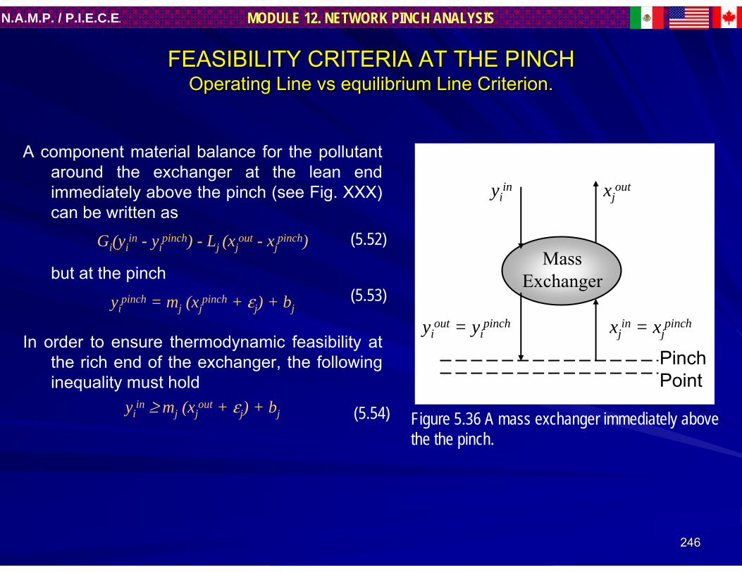
246246
MODULE 12. NETWORK PINCH ANALYSISN.A.M.P. / P.I.E.C.E.
A component material balance for the pollutant around the exchanger at the lean end immediately above the pinch (see Fig. XXX) can be written as
Gi(yiin - yi
pinch) - Lj (xjout - xj
pinch)
but at the pinch
yipinch = mj (xj
pinch + εj) + bj
In order to ensure thermodynamic feasibility at the rich end of the exchanger, the following inequality must hold
yiin ≥ mj (xj
out + εj) + bj
FEASIBILITY CRITERIA AT THE PINCHFEASIBILITY CRITERIA AT THE PINCHOperating Line Operating Line vsvs equilibrium Line Criterion.equilibrium Line Criterion.
yiin
yiout = yi
pinch
xjout
xjin = xj
pinch
PinchPoint
MassExchanger
(5.52)
(5.53)
(5.54) Figure 5.36 A mass exchanger immediately abovethe the pinch.

247247
MODULE 12. NETWORK PINCH ANALYSISN.A.M.P. / P.I.E.C.E.
Substituting from Eqs. (5.53) and (5.54) into Eq. (5.52), one getsGi[mj (xj
out + εj) + bj - mj(xjpinch + εj) - bj] ≤ Lj (xj
out - xjpinch)
and hence
ABOVE THE PINCH
(Lj / mj ) ≥ Gi
this is the feasibility criterion for matching a pair of streams (i, j) immediately above the pinch. That is, in order for a match immediately above the pinch to be feasible, the slope of the operating line should be greater than or equal to the slope of the equilibrium line.
BELOW OF PINCHOn the other hand, one can similarly show that the feasibility criterion for matching a pair
of streams (i, j) immediately below the pinch is given by
(Lj / mj ) ≤ Gi
Once again, stream splitting may be required to guarantee that criteria inequality is realized for each pinch match.
(5.55)
(5.56a)
(5.56b)

248248
MODULE 12. NETWORK PINCH ANALYSISN.A.M.P. / P.I.E.C.E.
The feasibility criteria (Eqs. 5.51 and 5.56) should be fulfilled only at the pinch. Once thepinch matches are identified, it generally becomes a simple task to complete the network design. Moreover, the designer always has the freedom to violate these feasibility criteria at the expense of increasing the cost of external MSAs beyond the MOC requirement.
SUMMARIZING
The feasibility criteria described by Eqs. (5.51) and (5.56) can be employed to synthesize a MEN which has the minimum number of
exchangers that satisfy the MOC solution.

249249
MODULE 12. NETWORK PINCH ANALYSISN.A.M.P. / P.I.E.C.E.
NETWORK SYNTHESISNETWORK SYNTHESIS
NETWORK REPRESENTATION
Waste streams are represented by vertical arrows running at the left of the diagram.
Compositions (expressed as weight ratios of the key component in each stream) are placed next to the corresponding arrow.
A match between two streams is indicated by placing a pair of circles on each of the streams and connecting them by a line.
Mass-transfer loads of the key component for each exchanger are noted in appropriate units (e.g. kg pollutant/s) inside the circles.
The pinch is represented by two horizontal dotted lines.

250250
MODULE 12. NETWORK PINCH ANALYSISN.A.M.P. / P.I.E.C.E.
ABOVE THE PINCHFirst criterion. Above the pinch, we have two waste streams and two MSAs. Hence,
minimum number of exchangers here can be calculated according to Eq. (5.49) as
UMOC, above the pinch = 2 + 2 - 1 = 3 exchangers
Immediately above the pinch, the number of rich streams is equal to the number of the MSAs, thus the feasibility criterion given by Eq. (5.51) is satisfied.
Second criterion. The second feasibility (Eq. 5.56a) criterion can be checked through Fig. 5.37. By comparing the values of Lj/mj with Gi for each potential pinch match, one can readily deduce that it is feasible to match S1 with either R1 or R2immediately above the pinch.Nonetheless, while it is possible to match S2 with R2, it is infeasible to pair S2 with R1immediately above the pinch.
Therefore, one can match S1 with R1 and S2 with R2 as rich end pinch exchangers.
NETWORK SYNTHESISNETWORK SYNTHESISFeasibility Criteria applied to Feasibility Criteria applied to DephenolizationDephenolization Case Study.Case Study.

251251
MODULE 12. NETWORK PINCH ANALYSISN.A.M.P. / P.I.E.C.E.
R1
R2S1
S2
PinchPoint
G1=2.00 kg/s G2=1.00 kg/s L1/m1=2.50 kg/s L2/m2=1.36 kg/s
Feasible
Feasible
Feasible
Infeasible!!
Matches above the pinch: criterion Lj/mj ≥ Gi
Figure 5.37 Feasibility criteria above the pinch for the dephenolization example.

252252
MODULE 12. NETWORK PINCH ANALYSISN.A.M.P. / P.I.E.C.E.
Mass-transfer loads between R1 and S1. When two streams are paired, the exchangeable mass is the lower of the two loads of the streams. For instance, the mass exchange loads of R1 and S1 are 0.0664 kg/s and 0.0380 kg/s, respectively. Hence, the mass exchangeable from R1 to S1 is 0.0380 kg/s.
Owing to this match, the capacity of S1 above the pinch has been completely exhausted and S1 may now be eliminated from any further consideration in the rich-end sub-problem.
Mass-transfer loads between R2 and S2. Similarly, 0.0132 kg/s of phenol will be transferred from R2 to S2 thereby fulfilling the required mass-exchange duty for R2above the pinch.
No mass must pass through the pinch. Both remaining loads of R1 and S2 above the pinch are equal (0.0284 kg/s). This is attributed to the fact that no mass is passed through the pinch.
Final design above the pinch. The two streams (R1 and S2) are, therefore, matched and the synthesis sub-problem above the pinch is completed. This rich-end design is shown in Fig. 5.38.

253253
MODULE 12. NETWORK PINCH ANALYSISN.A.M.P. / P.I.E.C.E.
0.0284
0.0380
0.0132 0.0132
0.0380
0.0284
R12.00 kg/s
R21.00 kg/s
0.0500
0.0358
0.0168
0.0300
0.0300
0.0164
0.0100PinchPoint
5.00 kg/sS1
2.08 kg/sS2
0.00740.0168
0.0150
Figure 5.38 The rich-end design for the dephenolization example.

254254
MODULE 12. NETWORK PINCH ANALYSISN.A.M.P. / P.I.E.C.E.
Intermediate composition. The intermediate compositions can be calculated through component material balance. For instance, the composition of S2 leaving its match with R2 and entering is match with R1, x2
intermediate, can be calculated via a material balance around the R2-S2 exchanger, I.e.,
or a material balance around the R1-S2 exchanger:
Having completed the design above the pinch, we can now move to the problem below the pinch.
0164.008.2
0132.00100.0teintermedia2 =+=x
0164.008.2
0284.00300.0teintermedia2 =−=x
(5.58)
(5.59)

255255
MODULE 12. NETWORK PINCH ANALYSISN.A.M.P. / P.I.E.C.E.
BELOW THE PINCHFirst criterion. Immediately below the pinch, only streams R1, R2 and S1 exist. Stream S3
does not reach the pinch point and, hence, will not be considered when the feasibility criteria of matching streams at the pinch are applied.Since, Nrb is 2 and Nlb is 1, inequality (Eq. 5.51b) is satisfied.
UMOC, below the pinch = 2 + 2 - 1 = 3 exchangers
Second criterion. As can see in Fig. Xxx Si cannot be matched with either R1 or R2 since L1/m1 is greater than G1and G2, Hence, S1 must be split into two branches: one to be matched with R1 and the other to be paired with R2.There are infinite number of ways through which L1 can be split so as to satisfy Eq(xxx) . Let us arbitrary split L1 in the same ratio of G1 to G2, I.e., to 3.33 and 1.67 kg/s. this split realizes the inequality (XXX) since 3.33/2 < 2 and 1.67/2 < 1.
NETWORK SYNTHESISNETWORK SYNTHESISFeasibility Criteria applied to Feasibility Criteria applied to DephenolizationDephenolization Case Study.Case Study.

256256
MODULE 12. NETWORK PINCH ANALYSISN.A.M.P. / P.I.E.C.E.
The remaining loads of R1 and R2 can now be eliminated by S3 (activated carbon).
Several configurations can be envisioned for S3:- A split design (Fig. 5.39)- A serial design in which S3 if first matched with R1 (Fig. 5.40)- A serial design in which S3 is first matched with R2 (Fig. 5.41).
It is worth pointing out that the number of exchangers below the pinch is four which is one more than UMOC, below the pinch . Once again, UMOC, below the pinch is just a lower bound on the number of exchangers and does not have to be exactly realized.

257257
MODULE 12. NETWORK PINCH ANALYSISN.A.M.P. / P.I.E.C.E.
0.0080 0.0080
0.0056
0.0040
0.0068
0.0040
0.0068 0.0056
R12.00 kg/s
R21.00 kg/s
5.00 kg/sS1
S3 = 0.1127 kg/s
0.0168
0.0128
0.0100
0.0168
0.0128
0.0060
0.0074 0.0074
0.00500.1100
0.0000
Figure 5.39 A lean-end design for the dephenolization example.

258258
MODULE 12. NETWORK PINCH ANALYSISN.A.M.P. / P.I.E.C.E.
0.0080 0.0080
0.0056
0.0040
0.0068
0.0040
0.0068
0.0056
R12.00 kg/s
R21.00 kg/s
5.00 kg/sS1
S3 = 0.1127 kg/s
0.0168
0.0128
0.0100
0.0168
0.0128
0.0060
0.0074 0.0074
0.0050
0.1100
0.0000
0.0497
Figure 5.40 A lean-end design for the dephenolization example.

259259
MODULE 12. NETWORK PINCH ANALYSISN.A.M.P. / P.I.E.C.E.
0.0080 0.0080
0.0040
0.0068
0.0040
0.0068
0.0056
R12.00 kg/s
R21.00 kg/s
5.00 kg/sS1
S3 = 0.1127 kg/s
0.0168
0.0128
0.0100
0.0168
0.0128
0.0060
0.0074 0.0074
0.0050
0.1100
0.0000
0.0497
0.0056
Figure 5.41 A lean-end design for the dephenolization example.

260260
MODULE 12. NETWORK PINCH ANALYSISN.A.M.P. / P.I.E.C.E.
Figure 5.42 A complete MOC network for the dephenolization example.
0.0380
0.0040
0.0080
0.0068 0.0056
0.0380
0.0284
0.0056
0.0080
0.0132
0.0068
0.0040
0.0132
0.0284
R1 = 2.00 kg/s
R2 = 1.00 kg/s
S1 = 5.00 kg/s
S3 = 0.1127 kg/s
S2 = 2.08 kg/s
Pinch Point
0.0500
0.0358
0.0168
0.0168
0.0128
0.0100
0.0300
0.0168
0.0168
0.0128
0.0060
0.0500
0.0074
0.0074
0.0150
0.0300
0.0164
0.0100
0.0000
0.1100

261261
MODULE 12. NETWORK PINCH ANALYSISN.A.M.P. / P.I.E.C.E.
IMPROVING THE PRELIMINAR NETWORK DESIGNSIMPROVING THE PRELIMINAR NETWORK DESIGNS
Based upon the basic principles of graphic theory, it can be shown that a minimum-utility pinched network will generally feature more than the target minimum number of exchanger units.
Any minimum-utility network will involve one unit more than the target minimum number of units. Hence, a cost-effective network design ought to include a tradeoff between the number of units (capital cost) and the external MSA’s (operating cost).
A procedure for the systematic reduction in the number of units involves the use of “mass-load loops” and “mass-loads paths”.

262262
MODULE 12. NETWORK PINCH ANALYSISN.A.M.P. / P.I.E.C.E.
Mass-load loops
A mass-load loop is a path connection which can be traced through a network by starting from an exchanger and returning back to the same exchanger. Generally, each extra unit will correspond to the existence of one independent loop. That is, by breaking a loop, one can eliminate one exchanger from the network.
Each loop is characterized with the possibility of shifting mass-exchange loads around the loop by subtracting a load from one exchanger and adding it back to another exchanger on the same stream, and so on around the loop.
As a design heuristic, it is recommended to break the loop by eliminating the exchanger with the smallest mass-exchange load. Nonetheless, it has to be noted that it may not be always possible to apply this heuristic because of thermodynamic considerations.

263263
MODULE 12. NETWORK PINCH ANALYSISN.A.M.P. / P.I.E.C.E.
Mass-load paths
A mass-load path is a continuous which strats with an external MSA and concludes with a process MSA. By shifting the loads along a path, one can add an excess amount of external MSA to replace an equivalent amount of process MSA.
Fig. 5.43 shows a example of reducing a network after using a mass-load path.
Figure 5.43 Network for the removal of hydrogen sulfide from COG. (a) Minimum-utility network (b) Reduced network after using a mass-load path to shift a load of 0.0050 kg/s from S1 to S2
1
2
3
4
R1
R2
S1
S2
Pinch7.00
5.10
3.10
0.10 0.03
0.10 0.01
0.06
0.35 0.07 0.020.0621
0.0050 0.0006 0.0001
1 3
4
R1
R2
S1
S2
7.00
5.10
3.10
0.10 0.03
0.01
0.06
0.12 0.11 0.020.0621
0.0006 0.0051
(a) (b)

264264
MODULE 12. NETWORK PINCH ANALYSISN.A.M.P. / P.I.E.C.E.
TIER I: FUNDAMENTALSTIER I: FUNDAMENTALS
11 HEAT RECOVERY NETWORKS (HEAT RECOVERY NETWORKS (HENsHENs).).
22 STEADY STATE SIMULATION of STEADY STATE SIMULATION of HENsHENs..
33 OPERABILITY ANALYSIS of OPERABILITY ANALYSIS of HENsHENs..
44 RETROFIT of RETROFIT of HENsHENs..
55 MASS EXCHANGE NETWORKS (MENs).4MASS EXCHANGE NETWORKS (MENs).4
66 OPERABILITY ANALYSIS of OPERABILITY ANALYSIS of MENsMENs..

265265
MODULE 12. NETWORK PINCH ANALYSISN.A.M.P. / P.I.E.C.E.
6 MASS EXCHANGE NETWORK OPERABILITY 6 MASS EXCHANGE NETWORK OPERABILITY ANALYSISANALYSIS
The synthesis of a MEN was originally only targeted on minimizing a total annualized cost. However, it is been recognized that operational aspects must be taken into in account during process design.
Notwithstanding the value of these MENs synthesis, they share a common limitation: all of them are based on designing the MEN for nominal operating conditions.
One of the most serious challenges for the design of waste-management systems is the potential variations in waste flowrate and others characteristics as inlet concentrations streams.
As it was mentioned in HENs operability analysis section, typical de-bottlenecking practices for HENs include modifications to surface area and heat transfer coefficients. Now, de-bottlenecking practices will be required for MENs when changes to normal operating conditions (as change in flowrate and/or compositions) resulting in operability problems.

266266
MODULE 12. NETWORK PINCH ANALYSISN.A.M.P. / P.I.E.C.E.
The operability analysis for Mass Exchanger Networks start from optimal design, the solution for Minimum Operational Cost (MOC).
Starting from thermal effectiveness-NTU model developed in previous sections 2 and 3 is posed in this section a similar model to operability analysis of MENs. A equivalent concept to thermal effectiveness will be used here for develop the MENs operability analysis Model. This concept is called “mass effectiveness”.
Key concepts about the similar model for MENs will be given in this section and the students have to develop the details in order to reach the operability analysis required in the Open-Ended section (Tier III)

267267
MODULE 12. NETWORK PINCH ANALYSISN.A.M.P. / P.I.E.C.E.
MASS EFFECTIVENESS MASS EFFECTIVENESS ‘‘ηη’’
Exchanger Mass Effectiveness represents the ratio of the actual mass load exchanged of rich stream to the maximum load that is thermodynamically possible.
From Fig. 6.1(b) the actual mass exchanged of rich stream is
MG = G(y1 - y2)and for lean stream
ML = FL (xjout - xj
in)but applying the corresponding compositions
scales the E. ( ) isML = L (y4
* - y3*)
where L = FL/mj
The maximum mass load thermodynamically possible corresponds to inlet concentrations exchanger in both streams (y1, y*
3).The Equation for Exchanger Mass effectiveness is
η = (y1 - y2)/(y1 - y*3)
Figure 6.1 Schematic representation of a mass exchanger
(6.1)
(6.2)
(6.3)
(6.4)
R1
S1
Giy1
y2Ljy*
3
y*4
MassExchanger
Gi, yiin Gi, yi
out
Lj , xjinLj , xj
out
(a)
(b)
R1

268268
MODULE 12. NETWORK PINCH ANALYSISN.A.M.P. / P.I.E.C.E.
When the value of mass effectiveness and inlet concentrations of each are given then the outlet concentration of rich stream can be known by Eq. (6.4) expressed as
y2 = y1 - η (y1 - y*3)
By other hand, combining the Eq. (6.5) with a mass total balance around the exchanger we can obtain an equation for outlet concentration of lean stream
y*4 = y*
3 + λ η (y1 - y*3)
where λ = G/LThe Equations (6.5) and (6.6) can be used to calculate the outlet concentrations of two
streams in the mass exchanger and they represent the basic equations to elaborate a mathematics model required for operability analysis of MENs.
EQUATIONS FOR A MASS EXCHANGEREQUATIONS FOR A MASS EXCHANGER
(6.5)
(6.6)

269269
MODULE 12. NETWORK PINCH ANALYSISN.A.M.P. / P.I.E.C.E.
For a system to be fully defined, the number of variables must be equal to the number of equations. In this case of an existing mass exchanger network, the equations that can be written are
NV = S +2Iwhere
NV = Number of variablesS = Number of streamsI = Number of mass exchangers
The exchanger in Fig. 6.1 has NV = 4 that mean four equations are required to system to be fully defined. One equation comes from mass effectiveness (Eq. 6.5) and other from total mass balance (Eq. 6.6). The other two equations are the corresponding inlet concentrations of each stream, which are known from initial data. The system equation can be represented by following matrix
TOTAL NUMBER OF VARIABLES IN A NETWORKTOTAL NUMBER OF VARIABLES IN A NETWORK

270270
MODULE 12. NETWORK PINCH ANALYSISN.A.M.P. / P.I.E.C.E.
Other equation required to operability analysis of MENs as Height of differential contactor (H) and overall number of transfer units (NTU), may be taken from section 5.1.3 “Design of individual mass exchange”.
OTHERS DESIGN EQUATIONS OF MASS EXCHANGERSOTHERS DESIGN EQUATIONS OF MASS EXCHANGERS

271271
MODULE 12. NETWORK PINCH ANALYSISN.A.M.P. / P.I.E.C.E.
End of Tier IEnd of Tier I
Congratulations, you have worked hard and completed the reading, this is the end of Tier I. Yes I know there was much information and may be looks confused. However, in the next Tier you will see the application of these fundamentals and your doubts will become clearer.

272272
MODULE 12. NETWORK PINCH ANALYSISN.A.M.P. / P.I.E.C.E.
STRUCTURE:STRUCTURE:
TIER I. FUNDAMENTALSTIER I. FUNDAMENTALS
TIER II. CASES STUDYTIER II. CASES STUDY
TIER III. OPEN ENDEN PROBLEMSTIER III. OPEN ENDEN PROBLEMS

TIER IITIER II

274274
MODULE 12. NETWORK PINCH ANALYSISN.A.M.P. / P.I.E.C.E.
Tier II: Statement of IntentTier II: Statement of IntentThe goal of this Tier is the presentation of the design experience to emphasize
the inter-relationship of the foundation principles given in Tier I. This is to apply concepts and rules about Pinch Network Analysis in order to analyze and achieve improvement of industry process in saving energy andminimize operating costs.
Cases studies will be developed mainly on two subjects:– Steady sate simulation and Operability of HENs.– Mass Exchange Networks Operability and design of MENs.
The purpose is to teach fundamentals in Pinch Analysis over an existing network without simulation.
At the end of Tier II the student should have the basic understanding of HENsand MENs behavior and its relation to the problem of plant operability and suggest solutions.

275275
MODULE 12. NETWORK PINCH ANALYSISN.A.M.P. / P.I.E.C.E.
2.1 Worked Example of Steady State Simulation 2.1 Worked Example of Steady State Simulation of of HENsHENs..
Problem description.Problem description.The worked example for the steady state response analysis has beThe worked example for the steady state response analysis has been extracted from an en extracted from an
aromatics plant. The existing heat recovery network is describedaromatics plant. The existing heat recovery network is described below:below:–– 4 hot streams4 hot streams–– 6 cold streams6 cold streams–– 3 coolers3 coolers–– 2 heaters2 heaters–– 9 heat exchangers9 heat exchangers
In the Grid Diagram C1, C2, and C3 represent coolers and H1 and In the Grid Diagram C1, C2, and C3 represent coolers and H1 and H2 represent H2 represent heaters.heaters.

276276
MODULE 12. NETWORK PINCH ANALYSISN.A.M.P. / P.I.E.C.E.
Simplified flow sheet of Aromatic Plant.Simplified flow sheet of Aromatic Plant.
E-1
E-1
E-1
Crude AromaticProduct
Feed
H1R1
H2 H3
E1
E2
E3E4
E5
E6
E7 E8
E9
C1
C2
C3
R2 R3
X
F1
F2
D1
D2
P1
Figure 2.1 Simplified flowsheet of Aromatic plant.

277277
MODULE 12. NETWORK PINCH ANALYSISN.A.M.P. / P.I.E.C.E.
Grid Diagram of Existing Heat Recovery NetworkGrid Diagram of Existing Heat Recovery Network
5
6
7
8
9
10
T14
T17
T19
T23
T25
T27
Fig. 2.2 Heat Exchanger Network for Case Base.
2T4
3T6
4T11
1T1
T5
T22
E3
T16
E1T3 T2
T18
E2
T7
T21
E4T8
T15
E5
T12
T20
E6T9
T24
E7T10
T28
E8
T13
T26
E9
C1
C2
C3
H1
H2

278278
MODULE 12. NETWORK PINCH ANALYSISN.A.M.P. / P.I.E.C.E.
New RequirementsNew RequirementsThe throughput of the plant is to be increased by 20%.The throughput of the plant is to be increased by 20%.
It is desired to deIt is desired to de--bottleneck the process to maintain feasible operation under new bottleneck the process to maintain feasible operation under new campaign.campaign.
It is also required that operation for the base case conditions It is also required that operation for the base case conditions must be feasible as an must be feasible as an alternative option.alternative option.
It is assumed that during the new campaign, the inlet temperaturIt is assumed that during the new campaign, the inlet temperature of stream 1 is set e of stream 1 is set to 365 to 365 ooCC..
Limitations on installed utility capacity dictate that the critiLimitations on installed utility capacity dictate that the critical target temperatures cal target temperatures under new conditions are:under new conditions are:
For TFor T33 ;; 42 42 ≤≤ TT33 < 51 < 51 ooCC. . For TFor T55 :: TT55 = 303 = 303 ooCC..For TFor T1010 ;; 85 85 ≤≤ TT1010 < 107 < 107 ooCC..For TFor T2626 ;; 145 145 ≤≤ TT2626 < 173 < 173 ooCC..For TFor T2828 ;; 82 82 ≤≤ TT2828 < 128 < 128 ooCC. .
During normal operation the conditions for Temperature targetDuring normal operation the conditions for Temperature target of stream 5 is of stream 5 is ≥≥ 256 256 ooCC

279279
MODULE 12. NETWORK PINCH ANALYSISN.A.M.P. / P.I.E.C.E.
5
6
7
8
9
10
T14
T17
T19
T23
T25
T27
2T4
3T6
4T11
1T1
T5
T22
E3
T16
E1T3 T2
T18
E2
T7
T21
E4T8
T15
E5
T12
T20
E6T9
T24
E7T10
T28
E8
T26
E9
C1
C2
C3
H1
H2
42 ≤ T3 < 51 oCT5 = 303 oC
85 ≤ T10 < 95 oC
68 ≤ T13 < 74 oC
T13 290 ≤ T16 < 300 pC
111 ≤ T16 < 127 pC
380 ≤ T22 < 468 pC87 ≤ T24 < 107 pC
145 ≤ T26 < 173 pC82 ≤ T28 < 128

280280
MODULE 12. NETWORK PINCH ANALYSISN.A.M.P. / P.I.E.C.E.
Base Case InformationBase Case Information
85598014035102222220495327T27T25T23T19T17T14T11T6T4T1Supply Temperature (oC)
45.927.734.389.531.248.533.353.86040.64Flow rate (kg/s)
10987654321Stream No.
Fouling factor(m2 oC/W)
Heat transfer Coefficient(W/m2 oC)
Cp(J/kg oC)
Fouling factor(m2 oC/W)
Heat transfer Coefficient(W/m2 oC)
Cp(J/kg oC)
Stream Stream
0.0001180.0001090.0001650.0002140.0000960.0003790.0004500.0003660.000495
852232940.000118852260091501.4E9906421730.000109906260010649.7E8610445530.00016561026008346.3E7934260070.00021493426004186.12E61046374430.000096104626005143.34E5998216770.000379998260031276.9E4774260020.00045077417067928.46E3812314110.000366812260061237.6E2608249050.000492608260011207.4E1
Shell sideTube sideArea(m2)
Exchanger
Table 2.1 Stream data for base case
Table 2.2 Heat exchanger data.

281281
MODULE 12. NETWORK PINCH ANALYSISN.A.M.P. / P.I.E.C.E.
Calculating the network temperatures for the base case.Calculating the network temperatures for the base case.
Variables and equationsVariables and equations..Applying Eq. (2.4) of Tier I to the network of Fig. 2.2, the number of variables we have is
(NV),
In this case: S = 10, E = 9 M = 0 and BP = 0. Therefore NV = 28 Variables.Now the knows equations are:
o All supply temperatures are known, there are 10 streams so 10 equations.o Two equations (effectiveness and heat balance) by each heat exchanger: 2x9 =
18. 18 equations.o Mass balance about each stream split: in this case there is not split stream and
we have zero equations here.o The j – 1 known flow fraction gives one equation: in this case we have zero
equations here.o Mass balance about each mixing point gives one equation: in this case we have
no mixing points and also we have zero equations here.Finally we have 28 equations.Our system of equations is contains 28 variables (10 known and 18 unknown) and 28
equations (10 equations from inlet temperatures known and 18 will be generated for each heat exchanger).
BPMESNV 22 +++= (2.4)

282282
MODULE 12. NETWORK PINCH ANALYSISN.A.M.P. / P.I.E.C.E.
E1: HEAT EXCHANGER 1.E1: HEAT EXCHANGER 1.From Effectiveness equation:From Effectiveness equation:T2 = (1 - ε)T1 + εT15
From heat balance about heat exchangerFrom heat balance about heat exchangerT16 = CεεTT11 + (1+ (1--C C εε)T)T1515
E4: HEAT EXCHANGER 4.E4: HEAT EXCHANGER 4.From Effectiveness equation:From Effectiveness equation:T7 = (1 - ε)T6 + εT20
From heat balance about heat exchangerFrom heat balance about heat exchangerT21 = CεεTT66 + (1+ (1--C C εε)T)T2020
1
5
T1T2
T15 T16
E1
3
7
T6T7
T20 T21
E4
Generation of equationsGeneration of equations..The equations are generated as described in the section 2.2 “Response Equations”. In
order to show the procedure, the equations of only four heat exchangers will be developed.

283283
MODULE 12. NETWORK PINCH ANALYSISN.A.M.P. / P.I.E.C.E.
E6: HEAT EXCHANGER 6.E6: HEAT EXCHANGER 6.From Effectiveness equation:From Effectiveness equation:T12 = (1 - ε)T11 + εT19
From heat balance about heat exchangerFrom heat balance about heat exchangerT20 = CεεTT1111 + (1+ (1--C C εε)T)T1919
E8: HEAT EXCHANGER 8E8: HEAT EXCHANGER 8..From Effectiveness equation:From Effectiveness equation:T10 = (1 - ε)T9 + εT27
From heat balance about heat exchangerFrom heat balance about heat exchangerT28 = CεεTT99 + (1+ (1--C C εε)T)T2727
4
7
T11T12
T19 T20
E6
3
10
T9T10
T27 T28
E8

284284
MODULE 12. NETWORK PINCH ANALYSISN.A.M.P. / P.I.E.C.E.
System of Equations.
11 TT11 = 327= 32722 TT22 = (1 = (1 -- εε)T)T11 + + εεTT1515
33 TT33 = (1 = (1 -- εε)T)T22 + + εεTT1717
44 TT44 = 495= 49555 TT55 = (1 = (1 -- εε)T)T44 + + εεTT2121
66 TT6 6 = 220= 22077 TT77 = (1 = (1 -- εε)T)T66 + + εεTT2020
88 TT88 = (1 = (1 -- εε)T)T77 + + εεTT1414
99 TT99 = (1 = (1 -- εε)T)T88 + + εεTT2323
1010 TT1010 = (1 = (1 -- εε)T)T99 + + εεTT2727
1111 TT1111 = 222= 2221212 TT1212 = (1 = (1 -- εε)T)T1111 + + εεTT1919
1313 TT1313 = (1 = (1 -- εε)T)T1212 + + εεTT2525
1414 TT1414 = 102= 102
1515 T15 = CεT7 + (1 - Cε)T14
16 T16 = CεT1 + (1 - Cε)T15
17 T17 = 3518 T18 = CεT2 + (1 - Cε)T17
19 T19 = 14020 T20 = CεT11 + (1 - Cε)T19
21 T21 = CεT6 + (1 - Cε)T20
22 T22 = CεT4 + (1 - Cε)T21
23 T23 = 8024 T24 = CεT8 + (1 - Cε)T23
25 T25 = 5926 T26 = CεT12 + (1 - Cε)T25
27 T27 = 8528 T28 = CεT9 + (1 - Cε)T27

285285
MODULE 12. NETWORK PINCH ANALYSISN.A.M.P. / P.I.E.C.E.
Solution of System of Equations.Solution of System of Equations.
The network temperatures for the base case which have been calculated solving the system of equations are shown in Table 2.3.
T1 = 327 T8 = 142 T15 = 117 T22 = 383
T2 = 167 T9 = 104 T16 = 257 T23 = 80
T3 = 45 T10 = 89 T17 = 35 T24 = 94
T4 = 495 T11 = 222 T18 = 113 T25 = 59
T5 = 303 T12 = 179 T19 = 140 T26 = 161
T6 = 220 T13 = 69 T20 = 156 T27 = 85
T7 = 166 T14 = 102 T21 = 195 T28 = 93
Table 2.3 Heat exchanger network temperatures for base case conditions.

286286
MODULE 12. NETWORK PINCH ANALYSISN.A.M.P. / P.I.E.C.E.
Network Response After ModificationsNetwork Response After ModificationsThe network response is simulated after modification of flow rates and the inlet
temperature of stream 1. With the flow rates modification, the effectiveness must be up date by the equation 2.3 Tier I and the results for network supply and target temperatures for new operating conditions are shown in Table 2.4
Stream No. Supply temperature
Target temperature
Temperature requirements
1 T1 = 365 T3 = 49 42 ≤ T3 < 51 2 T4 = 495 T5 = 308 T5 = 303 3 T6 = 220 T10 = 91 85 ≤ T10 < 95 4 T11 = 222 T13 = 71 68 ≤ T13 < 74 5 T14 = 102 T16 = 277 290 ≤ T16 < 300 6 T17 = 35 T18 = 118 111 ≤ T18 < 127 7 T19 = 140 T22 = 376 380 ≤ T22 < 468 8 T23 = 80 T24 = 94 87 ≤ T24 < 107 9 T25 = 59 T26 = 162 145 ≤ T26 < 173 10 T27 = 85 T28 = 95 82 ≤ T28 < 128
Table 2.4. Network supply and target temperatures for new operating conditions.

287287
MODULE 12. NETWORK PINCH ANALYSISN.A.M.P. / P.I.E.C.E.
Response Simulation AnalysisResponse Simulation Analysis
The temperature response analysis will show what temperatures values are within acceptable bounds. Figure 2.3 shows the streams that fall outside bounds. . Figure 2.3 shows the streams that fall outside bounds.
Fig. 2.3 Target temperatures on acceptable bounds review.
UpperBound
LowerBound
51
T(oC)
Stream No.
49
1
42 303
303
T5 = 308
85
95
91
2 3 4 5 6 7 8 9 10
68
74
71
T16 = 277
290
300
111
127
118
380
468
T22 = 37687
107
94
162
145
173
82
128
95
is 5 oC above Tt
T5
is 13 oC below Tt
T16
is 4 oC below Tt
T22
Acce
ptable
Boun
d
Tt outsideacceptable boundTt withinacceptable bound

288288
MODULE 12. NETWORK PINCH ANALYSISN.A.M.P. / P.I.E.C.E.
Taking actions. Option 1.Taking actions. Option 1.
Streams 2 and 7.Streams 2 and 7.Stream 2 matches with stream 7 by Exchanger 3 (E3). In each stream its target
temperatures is outside of acceptable bounds.
This is the case of a hot stream falling above the upper bound. The way to restore the target temperature of stream 2 is by increasing the heat exchanger area of E3.
This action also benefits stream 7. However, for the target temperature of stream 7 to be acceptable, more heat is needed. Exchanger E6 is chosen and more area added.
Stream 5.Stream 5.Stream 5 enters exchanger E5 first and E1 afterward. After E1 stream temperature (T16)
is 13 oC below the target temperature required by the process.
This is the case of a cold stream falling below the lower bound. The solution is to increase the heat exchanger area.
Increasing area on exchangers E1 and E5 restores the target temperature of stream 5.

289289
MODULE 12. NETWORK PINCH ANALYSISN.A.M.P. / P.I.E.C.E.
Network simulation after corrective actionsNetwork simulation after corrective actions
The solution results for additional surface area and network temperatures after the exchangers have been modified are presented in Tables 2.4 and 2.5 respectively.
Exchanger No. Additional area (m2)
E1 1534 E3 1002.6 E5 291.3 E6 239.6
Table 2.5 Heat transfer area requirementson exchangers E1, E3 and E6.

290290
MODULE 12. NETWORK PINCH ANALYSISN.A.M.P. / P.I.E.C.E.
Stream No. Supply temperature
Target temperature
Temperature requirements
1 T1 = 365 T3 = 48 42 ≤ T3 < 51 2 T4 = 495 T5 = 303.3 T5 = 303 3 T6 = 220 T10 = 89.4 85 ≤ T10 < 95 4 T11 = 222 T13 = 70.4 68 ≤ T13 < 74 5 T14 = 102 T16 = 290.9 290 ≤ T16 < 300 6 T17 = 35 T18 = 115 111 ≤ T18 < 127 7 T19 = 140 T22 = 381.7 380 ≤ T22 < 468 8 T23 = 80 T24 = 91.2 87 ≤ T24 < 107 9 T25 = 59 T26 = 156.6 145 ≤ T26 < 173 10 T27 = 85 T28 = 92.4 82 ≤ T28 < 128
Table 2.6 Stream supply and target temperatures for new operatingConditions and increasing area on exchangers E1, E3, E5 and E6.

291291
MODULE 12. NETWORK PINCH ANALYSISN.A.M.P. / P.I.E.C.E.
UpperBound
LowerBound
51T(oC)
Stream No.
48
1
42 303
303.3
85
95
89.4
2 3 4 5 6 7 8 9 10
68
74
70.4 290.9290
300
111
127
115
380
468
381.787
107
91.2156.6
145
173
82
128
92.2Acce
ptable
Boun
d
Tt within acceptable bound
303
Response Simulation Analysis after exchanger modificationsResponse Simulation Analysis after exchanger modifications
Solution results for additional surface are and network temperatures after the exchangers have been modified.

292292
MODULE 12. NETWORK PINCH ANALYSISN.A.M.P. / P.I.E.C.E.
Corrective actions. Option 2.Corrective actions. Option 2.
Stream 7.Stream 7.The restoration of target temperature of stream 7 can be accomplished by modification
of exchangers E3, E4 and E6.
Heat exchangers with a high thermal effectiveness require larger amount of additional surface area to achieve a certain response on outlet temperatures whereas low effectiveness exchangers achieve the same response with less additional area. In this case, the thermal effectiveness of exchangers E3, E4 and E6 for the base case are 0.64, 0.84 and 0.52 respectively. Therefore, the designer should start his analysis by considering the exchangers with the lower thermal effectiveness that in this case are E3 and E6.
Another element that needs to be considered in the solution of cases like this, is that the interaction between exchangers call for a strategic order of modifications. This is, if target temperature of stream 7 is to be restored, E6 must be analyzed first, followed by E4 and then E3.

293293
MODULE 12. NETWORK PINCH ANALYSISN.A.M.P. / P.I.E.C.E.
Simulation the revised network when operating conditions Simulation the revised network when operating conditions return to normal.return to normal.
From the results shown in Table 2.6, the only target temperature that is now out of specification is T5, the outlet temperature of stream 2.
Analyzing structure it is clear that the restoration of this controlled variable can be achieved by reducing the heat load of E3. So, a bypass must be implemented here. It is found that by allowing 10 % of the flow rate of stream 2 through the bypass, temperature T5 reaches the required condition.
The simulation results are shown in Table 2.7.
Fig. 2.5 Heat exchanger 3 with bypass.
T4T5
T21
BP = ByPass
r2.1 = 0.10
M
T22
r2.2 = 0.902
BPE3

294294
MODULE 12. NETWORK PINCH ANALYSISN.A.M.P. / P.I.E.C.E.
Stream No. Supply temperature
Target temperature
Temperature requirements
1 T1 = 327 T3 = 44.3 42 ≤ T3 < 51 2 T4 = 495 T5 = 303 T5 = 303 3 T6 = 220 T10 = 87.9 85 ≤ T10 < 95 4 T11 = 222 T13 = 68.5 68 ≤ T13 < 74 5 T14 = 102 T16 = 268.2 T16 ≥ 256 6 T17 = 35 T18 = 111.2 111 ≤ T18 < 127 7 T19 = 140 T22 = 391.1 380 ≤ T22 < 468 8 T23 = 80 T24 = 91.2 87 ≤ T24 < 107 9 T25 = 59 T26 = 155.3 145 ≤ T26 < 173 10 T27 = 85 T28 = 91.2 82 ≤ T28 < 128
Table 2.7 Stream supply and target temperatures with increased areaon E1, E3, E5 and E6 and restored original operating conditions.Bypass on exchanger E3.

295295
MODULE 12. NETWORK PINCH ANALYSISN.A.M.P. / P.I.E.C.E.
Response Analysis. Simulation after revised network.Response Analysis. Simulation after revised network.
The response analysis shows that all target temperatures are within acceptable bounds after corrective actions have been taken..
Fig. 2.4 Target temperatures are all within acceptable bounds after correctives actions.
UpperBound
LowerBound
51
T(oC)
Stream No.
48
1
42 303
303
303
85
95
89.4
2 3 4 5 6 7 8 9 10
68
74
70.4209.9
290
300
111
127
115
380
468
381.7
87
107
91.2156.6
145
173
82
128
92.2Acce
ptable
Boun
d
Tt within acceptable bound

296296
MODULE 12. NETWORK PINCH ANALYSISN.A.M.P. / P.I.E.C.E.
The model for the steady state simulation of a single phase heat recovery networks is based on the development of a system of steady state linear equations: these include the thermal effectiveness and the heat balance of every exchanger, the heat balance about the mixing points and the mass balance about stream split points present in the network.
In this case study it is shown how to retrofit an existing heat exchanger network to operate under conditions different from the original design and deliver target temperatures that meet the process requirements. The final network is said to be FLEXIBLE and OPERABLE. The retrofit of the existing network to achieved by the incorporation of additional surface area and the use of bypasses.
The method includes the assessment of the network response to modified (hA). This is done by updating the heat transfer coefficient to variations in stream flow rate.

297297
MODULE 12. NETWORK PINCH ANALYSISN.A.M.P. / P.I.E.C.E.
Design for operabilityDesign for operability..
All Tt streams are within acceptable bounds?
NETWORK SIMULATION RESTOREDORIGINAL OPERATING CONDITIONS
All Tt streams are within acceptable bounds?
HEAT RECOVERY NETWORK OPERABLE AND FLEXIBLE
TAKE CORRECTIVEACTIONS
TAKE CORRECTIVEACTIONS
Yes
Yes
No
No
RESPONSE
RESPONSE
ANALYSIS
ANALYSIS
SIMULATION
-- Increased Area-- Bypass
-- Increased Area-- Bypass
NEW REQUIREMENTS
T UNKNOWN CALCULATION
MODEL
EXISTING HEAT RECOVERY NETWORK -Problem description-Grid Diagram--Flow sheet-- Stream and heat exchanger dataset
System of Equations
Solution of equation system

298298
MODULE 12. NETWORK PINCH ANALYSISN.A.M.P. / P.I.E.C.E.
STRUCTURE:STRUCTURE:
TIER I. FUNDAMENTALSTIER I. FUNDAMENTALS
TIER II. CASES STUDYTIER II. CASES STUDY
TIER III. OPEN ENDEN PROBLEMSTIER III. OPEN ENDEN PROBLEMS

TIER IIITIER III
OPEN ENDED PROBLEM

300300
MODULE 12. NETWORK PINCH ANALYSISN.A.M.P. / P.I.E.C.E.
Tier III: Statement of IntentTier III: Statement of Intent
The goal of this Tier is for students to solve to exercise theirThe goal of this Tier is for students to solve to exercise their ability to integrate ability to integrate methods and technologies about operability analysis in existing methods and technologies about operability analysis in existing heat heat exchange networks and mass exchange networks that have been taugexchange networks and mass exchange networks that have been taught ht from Fundamentals (Tier I) and Study Cases (Tier II) sections infrom Fundamentals (Tier I) and Study Cases (Tier II) sections in this this Module.Module.
The solution of open ended problems involves to reaching severalThe solution of open ended problems involves to reaching several or many or many correct answers, and several ways to the correct correct answers, and several ways to the correct answer(sanswer(s) depending of ) depending of approach used. It is important not only to show final results, bapproach used. It is important not only to show final results, but also to ut also to explain how students got their answers or why they chose the metexplain how students got their answers or why they chose the method they hod they did.did.

301301
MODULE 12. NETWORK PINCH ANALYSISN.A.M.P. / P.I.E.C.E.
Tier III. ContentsTier III. Contents
Tier III is broken down into two sections.Tier III is broken down into two sections.11 Operability analysis for a Heat Exchange NetworkOperability analysis for a Heat Exchange Network
22 Operability analysis for a Mass Exchange NetworkOperability analysis for a Mass Exchange Network

302302
MODULE 12. NETWORK PINCH ANALYSISN.A.M.P. / P.I.E.C.E.
OPEN ENDED PROBLEMOPEN ENDED PROBLEM
Operability Analysis for a Heat Exchange Operability Analysis for a Heat Exchange Network.Network.

303303
MODULE 12. NETWORK PINCH ANALYSISN.A.M.P. / P.I.E.C.E.
Operability Analysis for a Heat Exchange Network.Operability Analysis for a Heat Exchange Network.
Problem statement.Problem statement.The open ended problem for the HEN operability analysis is about the same aromatics
plant worked in the Study Cases (Tier II) section. The existing heat recovery network requires to be retrofitted for 120 % throughput (relative to existing capacity) and reach new target temperatures in some streams. These new target temperatures are:
– Inlet temperature to exchanger X which must be kept at 307 oC (Stream 2)– Inlet temperature to Reactor R1 (Stream 5)– Feed to distillation column D1 whose minimum allowable bound is 164 oC (Stream 6)– Inlet temperature to Reactor R2 (stream 7)– Feed to distillation column D2 whose minimum allowable bound is 152 oC (Stream 9)
Another constraint that adds to the problem is that furnaces H1 and H2 have maximum firing capacities that must be observed. These are:
– H1, 8 300 kW– H2, 19 400 kW
In the Figures 3.1 and 3.2 are shown the flowsheet and grid diagram respectively of aromatic plant that will be worked for operability analysis.

304304
MODULE 12. NETWORK PINCH ANALYSISN.A.M.P. / P.I.E.C.E.
Simplified flow sheet of Aromatic Plant.Simplified flow sheet of Aromatic Plant.
Figure 3.1 Simplified flowsheet of Aromatic plant.
E-1
E-1
E-1
Crude AromaticProduct
TreatedNaphtaFeed
H1R1
H2 H3
E1
E2
E3E4
E5
E6
E7 E8
E9
C1
C2
C3
R2 R3
X
F1
F2
D1
D2
P1

305305
MODULE 12. NETWORK PINCH ANALYSISN.A.M.P. / P.I.E.C.E.
Grid Diagram of Existing Heat Recovery NetworkGrid Diagram of Existing Heat Recovery Network
Fig. 3.2 Grid representation of exchanger network of aromatic plant.
5
6
7
8
9
10
T14
T17 T19
T23 T25 T27
2
T4
3
T6
4
T11
1T1
T5
T22
E3
T16
E1T3 T2
T18
E2
T7
T21
E4T8
T15
E5T12
T20
E6
T9
T24
E7T10
T28
E8
T13
T26
E9
C1
C2
C3
Inlet to exchanger X
Outlet fromExchanger X
T29
T30 T31
T32 T33
H1
H2

306306
MODULE 12. NETWORK PINCH ANALYSISN.A.M.P. / P.I.E.C.E.
Task Design.Task Design.Solve operability problem for exposed process through finding critical exchangers within
network and apply the appropriate corrective actions (additional area or bypass) to ensure that all network temperatures are within acceptable bounds.
Develop different strategies to reach the required operability with new requirement and under normal operating conditions based on basics given into parts 2 and 3 of Tier I and methodology developed into Tier II.
Additional information about stream data for base case and heat exchanger data for solving this problem must be taken of the same process developed in Case Studies (Tier II)

307307
MODULE 12. NETWORK PINCH ANALYSISN.A.M.P. / P.I.E.C.E.
Steps for identify strategies to achieve the design taskSteps for identify strategies to achieve the design taskThe following steps may help you to the identification of strategies to achieve the
operability analysis task:– Specify all stream temperature bounds– Determine the steady state response of the network to imposed disturbances.– Produce the Heat Load Shift Table– Devise the strategy for the shifting of heat within the network. This is done in
conjunction with the actual network structure.– Determine order in which modifications should be undertaken– Apply corrective equations to calculate additional area (or, bypass) for the
various exchangers involved.

308308
MODULE 12. NETWORK PINCH ANALYSISN.A.M.P. / P.I.E.C.E.
OPEN ENDED PROBLEMOPEN ENDED PROBLEM
Operability Analysis for a Mass Exchange Operability Analysis for a Mass Exchange Network.Network.

309309
MODULE 12. NETWORK PINCH ANALYSISN.A.M.P. / P.I.E.C.E.
OPEN ENDED PROBLEM FOR THE DEPHENOLIZATION PROBLEM.OPEN ENDED PROBLEM FOR THE DEPHENOLIZATION PROBLEM.The open ended problem for MENs operability analysis is for a network resulting of
example problem worked in section 5.2.4 “Design to Minimum Number of Mass Exchanger units” of Tier I.
The network for operability analysis is shown in Fig. 3.3. It has two rich streams, one lean stream (external MSA), and two mass exchanger. New operating conditions are required to flowrate and stream composition. This disturbance will affect target composition.
Using fundamentals given in Tier I and methodology developed to study case in Tier II for HENs operability analysis develop in a similar way different solutions strategies to reach operability condition required for new operating condition in network given.

310310
MODULE 12. NETWORK PINCH ANALYSISN.A.M.P. / P.I.E.C.E.
0.0240 0.0800
R12.00 kg/s
R21.00 kg/s
S3 = 0.9455 kg/s
0.0500
0.0100
0.0300
0.0060
0.1100
0.0000
0.0240
0.0800
Figure 3.3 Network for the dephenolization open ended problem

311311
MODULE 12. NETWORK PINCH ANALYSISN.A.M.P. / P.I.E.C.E.
END OF TIER IIIEND OF TIER III
This is the end of Module 12. Please submit your report to your professor for grading.