programa de doctorado matemáticas phd dissertionat
TRANSCRIPT

Programa de doctorado �Matemáticas�
PhD Dissertation
CLASSIFICATION AND REGRESSION WITH
FUNCTIONAL DATA. A MATHEMATICAL
OPTIMIZATION APPROACH
Author
Ma Asunción Jiménez Cordero
Supervisors
Prof. Dr. Rafael Blanquero Bravo
Prof. Dr. Emilio Carrizosa Priego


some text to complete some text tocomplete
some text to completesome text to complete some text to
completesome text to complete some text to
completesome text to complete some text to
complete
A mis padres.
A mi hermana.


Agradecimientos
Me gustaría, en primer lugar, dar las gracias a todas las personas que han pasado por
mi vida, incluso a aquéllas que me han hecho pasar un mal rato. De una u otra forma,
habéis de�nido quién soy, y por todo eso esta tesis existe.
Para hacer una tesis no sólo hace falta tiza, pizarra, un ordenador y alguna que otra
idea. También es necesario, y mucho, personas a tu lado que te hagan más amenos
esos momentos en los que las cuentas no salen como a uno le gustaría. Por ello, quiero
dar las gracias a mis directores Rafa y Emilio, por la oportunidad que me han dado de
crecer no sólo como investigadora sino también como persona. He aprendido mucho con
vosotros. Rafa: gracias por esos ratos en tu despacho en los que, por n−ésima vez me
daba cuenta que si ponía los vectores por columnas en lugar de por �las, el código iba
más rápido, o por aquéllos momentos en los que nos planteábamos si hacíamos trampas
al solitario. Emilio: tú me descubriste como investigadora aquella tarde de hace ya más
de seis años en la que fui a pedirte un cambio de examen sin que ni siquiera fueras mi
profesor. Y miráme ahora, leyendo una tesis. Gracias.
Belén: te doy las gracias por enseñarme a ver las Matemáticas desde un punto
distinto al que estaba acostumbrada. Agradecer también a Richard y Sebastián su
dedicación y apoyo durante mi estancia. Richard: gracias por todo lo que aprendí en
esos tres meses. Sebastián: ya sabes que siempre ha sido un placer trabajar contigo.
Por supuesto dar las gracias a los compañeros del doctorado chileno, DSI. Weones, me
acogistéis como si me conocieráis de toda la vida, incluso antes de que llegara, y luego
allá, me enseñastéis que Chile es bacán y que tiene algo más que empanadas, terremotos
y pisco sour. Mil gracias.
Quiero dar las gracias al Departamento de Estadística e Investigación Operativa,
por permitirme dar clases en las que los alumnos no eran los únicos que aprendían.
En particular, gracias a Alicia, con quién compartir asignatura siempre fue un placer.
Muchas gracias también al equipo de soporte de supercomputación del CICA y del
CSIRC. Es admirable con la rapidez y e�cacia que contestásteis a todas las dudas que
me surgieron. Sin muchas de esas respuestas los experimentos computacionales de esta
tesis no se habrían llevado a cabo. Por todo ello, gracias.
Por supuesto no me puedo olvidar de agradecer esta tesis al equipo de Administración
IV

V
del IMUS. Hacéis un trabajo impecable, y cada vez estoy más convencida que sin vuestra
ayuda el IMUS se hundiría. En particular, mencionar a Adela, Clarines, Rafa, Teresa y
Víctor. Gracias por resolver, siempre con una sonrisa, los problemas (no matemáticos)
que os planteamos. Y hablando del IMUS, no me puedo olvidar de mencionar a mis
compis de doctorado, a los que están y a los que un día estuvieron. Sin vosotros, el día
a día sería muy distinto. Gracias por las risas de los cafés, por las cenas improvisadas, y
simplemente por estar ahí para celebrar los buenos ratos con dulces, y por compartir los
malos. Que no se os olvide: que lo que el IMUS ha unido, que no lo separen las post-docs.
En especial, dar las gracias a Alba por sus consejos de última hora, y a Cristina por ser la
alegría del doctorado. Gracias a Marina por sus risas, por ser la mejor compi de pasillo,
y la primera a la que le cuento todos los sinsentidos que me pasan. Gracias también
a Reme, quién más de una vez (y de dos) ha tenido que aguantar que me desahogue
con ella. Por supuesto, gracias a Tom. Although I am the worst you understand when
speaking, you are always there when I need it. Y gracias a ti Vanesa por ser mi guía
durante todo este tiempo. No te creas que esto se acaba aquí. Afortunadamente, aún
nos quedan muchos congresos (y otras cosas) por vivir juntas.
Me gustaría dar las gracias también a los Pijos, pan y habas. Israel, José, Marina:
los buenos momentos que pasamos en el Despacho 8 siempre se quedarán con nosotros.
Israel: eres único. Fuiste mi primer compi de despacho, y eres el mejor dejando que
los demás discutan, mientras tú y yo nos reímos. José: aunque seas un malaje, se te
coge cariño. Y mucho. Marina: ½qué suerte la mía cuando te cambiaste de grupo en el
primer año de carrera! Ha sido largo el camino que llevamos recorrido juntas, y aunque
a veces nos lo han puesto realmente difícil, hemos luchado codo con codo por nuestros
sueños (por ejemplo preinscribiendo a nuestras madres en el Máster de Matemáticas).
No puedo olvidarme de dar las gracias al resto de mis Fantásticas. Para nosotras el
in�nito siempre tendrá un signi�cado especial, aunque algunas lo llevemos con tinta
invisible. En particular, dar las gracias a Bea por ayudarme cuando más lo necesitaba,
y a Ana Happy por ser tan tú.
Dar las gracias a Gisela. Tus frases de buenos días y tu manera de ver la vida me
hacen ser más fuerte. Ana Mariam: nos conocimos en Sevilla, y al �nal hemos acabado
quedando en Madrid. Gracias por esos ratos en los que la una decía a la otra justo lo
que debía escuchar.
No hay su�cientes palabras con las que poder agradecerle a mi Pedro todo lo que ha
hecho por mí. Tú y yo sabemos que esta tesis es muchísimo más que unas cuantas de
páginas. Gracias por apoyarme en todo momento y por ayudarme, aunque no siempre
entendieras todo lo que pasaba. Gracias por enseñarme todo lo que sabías e incluso más.
Gracias por explicarme que en una libreta se pueden escribir mucho más que palabras.
Juntos hemos aprendido mucho, y seguiremos avanzando como el equipo que somos.
Aquí no se rinde nadie.

VI
Por último, dar las gracias a mi familia. Una vez me dijeron que tu familia, pase lo
que pase, siempre está. ½Qué gran verdad! Gracias a mis abuelos, a las que están cerca
y a los que me vigilan desde un poco más arriba. Vosotros me habéis mimado como
sólo los abuelos saben hacer. Gracias a mis padres, por enseñarme que con sacri�cio,
esfuerzo y trabajo todo, absolutamente todo, se consigue. Papá: gracias por tomarme
la lección de pequeña, por tu paciencia in�nita y por todas esas veces en las que tú
eras el que salías perdiendo. Mamá: somos iguales, y eso me enorgullece. Gracias por
enseñarme a no parar de luchar hasta que tu objetivo se haya cumplido. Gracias a mi
hermana. Andrea: eres lo más. Gracias por nuestras charlas y por tus consejos en los
que, a veces, no se sabía quién era la hermana mayor.
A todos, gracias.


Resumen
El objetivo de esta tesis doctoral es desarrollar nuevos métodos para la clasi�cación
y regresión supervisada en el Análisis de Datos Funcionales. En particular, las herra-
mientas de Optimización Matemática analizadas en esta tesis explotan la naturaleza
funcional de los datos, dando lugar a nuevas técnicas que pueden mejorar los métodos
clásicos y que conectan las matemáticas con las aplicaciones.
El Capítulo 1 presenta las ideas generales, los retos y la notación usada a lo largo
de la tesis.
El Capítulo 2 trata el problema de seleccionar el conjunto �nito de instantes de
tiempo que mejor clasi�ca datos funcionales multivariados en dos clases prede�nidas.
El uso, no sólo de la información proporcionada por la propia función, sino también por
sus derivadas será decisivo para mejorar la predicción, como se pondrá de mani�esto pos-
teriormente. Para ello se formula un problema de optimización binivel continuo. Dicho
problema combina la aplicación de la conocida técnica SVM (Support Vector Machine)
con la maximización de la correlación entre la etiqueta de la clase y la denominada
función score, vinculada a dicha técnica.
El Capítulo 3 también se centra en la clasi�cación binaria de datos funcionales
usando SVM. Sin embargo, en lugar de buscar los instantes de tiempo más relevantes,
aquí se de�ne un ancho de banda funcional para la denominada función kernel. De esta
forma, se puede mejorar el rendimiento del clasi�cador, a la vez que se identi�can los
diferentes intervalos del dominio de la función, de acuerdo a su capacidad predictiva,
mejorando además la interpretabilidad del modelo resultante. La obtención de tales
intervalos se lleva a cabo mediante la resolución de un problema de optimización binivel
por medio de un algoritmo alternante.
El Capítulo 4 se centra en la clasi�cación de los llamados datos funcionales híbridos,
es decir, datos que están formados por variables funcionales y estáticas (constantes a lo
largo del tiempo). El objetivo es seleccionar las variables, funcionales o estáticas, que
mejor clasi�quen. Para ello, se de�ne un kernel no isotrópico que asocia un parámetro
ancho de banda escalar a cada una de las variables. De forma análoga a como se ha
hecho en los capítulos anteriores, se propone un algoritmo alternante para resolver el
problema de optimización binivel, que permite resolver los parámetros del kernel.
VIII

IX
El problema de selección de variables presentado en el Capítulo 2 se generaliza al
campo de la regresión en el Capítulo 5. El método de resolución combina la técnica
denominada SVR (Support Vector Regression) con la minimización de la suma de los
cuadrados de los residuos entre la verdadera variable respuesta y la prevista.
Todos los algoritmos propuestos a lo largo de esta tesis han sido aplicados a bases
de datos sintéticas y reales, quedando probada su efectividad.

Summary
The goal of this PhD dissertation is to develop new approaches for supervised classi-
�cation and regression in Functional Data Analysis. Particularly, the Mathematical
Optimization tools analyzed in this thesis exploit the functional nature of the data,
leading to novel strategies which may outperform the standard methodologies and link
mathematics with real-life applications.
Chapter 1 presents the main ideas, challenges and the notation used in this thesis.
Chapter 2 addresses the problem of selecting a �nite set of time instants which best
classify multivariate functional data into two prede�ned classes. Using, not only the
information provided by the function itself but also its high-order derivatives will be
crucial to improve the accuracy. To do this, a continuous bilevel optimization problem
is solved. Such problem combines the resolution of the well-known technique SVM
(Support Vector Machine) with the maximization of the correlation between the class
label and the score.
Chapter 3 also focuses on the binary classi�cation problem using SVM. However,
instead of �nding the most important time instants, here we de�ne a functional band-
width in the so-called kernel function. In this way, accuracy may be improved and the
most relevant intervals of the domain of the function, according to their classi�cation
ability, are identi�ed, enhancing the interpretability. A bilevel optimization problem is
formulated and solved by means of an alternating procedure.
Chapter 4 is focused on classifying the so-called hybrid functional data, i.e., data
which are formed by functional and static (constant over time) covariates. The goal is
to select the features, functional or static, which best classify. An anisotropic kernel
which associates a scalar bandwidth to each feature is de�ned. As in previous chapters,
an alternating approach is proposed to solve a bilevel optimization problem.
Chapter 5 generalizes the variable selection problem presented in Chapter 2 to re-
gression. The solution approach combines the SVR (Support Vector Regression) problem
with the minimization of sum of the squared residuals between the actual and predicted
responses. An alternating heuristic is developed to handle such model.
All the methodologies presented along this dissertation are tested in synthetic and
real data sets, showing their applicability.
X


Contents
1 Introduction 1
1.1 Functional Data Analysis . . . . . . . . . . . . . . . . . . . . . . . . . . 4
1.2 Supervised Classi�cation and Regression . . . . . . . . . . . . . . . . . . 7
1.2.1 Supervised Learning . . . . . . . . . . . . . . . . . . . . . . . . . 8
1.2.2 Support Vector Machine (SVM) and Support Vector Regression
(SVR) . . . . . . . . . . . . . . . . . . . . . . . . . . . . . . . . . 10
1.2.3 Kernels De�nition . . . . . . . . . . . . . . . . . . . . . . . . . . 13
1.2.4 Performance Estimation . . . . . . . . . . . . . . . . . . . . . . . 15
1.3 Feature Selection . . . . . . . . . . . . . . . . . . . . . . . . . . . . . . . 16
1.4 Contributions of this Thesis . . . . . . . . . . . . . . . . . . . . . . . . . 18
2 Variable Selection in Functional Data Classi�cation with SVM 21
2.1 Introduction . . . . . . . . . . . . . . . . . . . . . . . . . . . . . . . . . . 23
2.2 A Global Optimization Approach to the Variable Selection Problem . . . 24
2.2.1 Variable Selection with Functional SVM . . . . . . . . . . . . . . 24
2.2.2 The Bilevel Optimization Problem . . . . . . . . . . . . . . . . . 25
2.2.3 A Nested Heuristic . . . . . . . . . . . . . . . . . . . . . . . . . . 28
2.2.4 Choice of the Number of Variables, H . . . . . . . . . . . . . . . 29
2.3 Numerical Experiments . . . . . . . . . . . . . . . . . . . . . . . . . . . 30
2.3.1 Description of the Experiments . . . . . . . . . . . . . . . . . . . 30
2.3.2 Description of the Data Sets . . . . . . . . . . . . . . . . . . . . . 30
2.3.3 Results . . . . . . . . . . . . . . . . . . . . . . . . . . . . . . . . 34
2.4 Conclusions and Extensions . . . . . . . . . . . . . . . . . . . . . . . . . 39
3 Bandwidth Selection in SVM with Functional Data 45
3.1 Introduction . . . . . . . . . . . . . . . . . . . . . . . . . . . . . . . . . . 47
3.2 Functional Bandwidth . . . . . . . . . . . . . . . . . . . . . . . . . . . . 47
3.3 Optimal Selection of the Functional Bandwidth . . . . . . . . . . . . . . 51
3.4 Numerical Experiments . . . . . . . . . . . . . . . . . . . . . . . . . . . 53
3.4.1 Description of the Experiments . . . . . . . . . . . . . . . . . . . 53
XII
Contents XIII
3.4.2 Description of the Data Sets . . . . . . . . . . . . . . . . . . . . . 55
3.4.3 Results . . . . . . . . . . . . . . . . . . . . . . . . . . . . . . . . 57
3.5 Conclusions and Extensions . . . . . . . . . . . . . . . . . . . . . . . . . 59
4 SVM-Classi�cation of Hybrid Functional Data 67
4.1 Introduction . . . . . . . . . . . . . . . . . . . . . . . . . . . . . . . . . . 69
4.2 The Mathematical Model . . . . . . . . . . . . . . . . . . . . . . . . . . 69
4.3 Numerical Experiments . . . . . . . . . . . . . . . . . . . . . . . . . . . 71
4.3.1 Description of the Experiments . . . . . . . . . . . . . . . . . . . 72
4.3.2 Description of the Data Sets . . . . . . . . . . . . . . . . . . . . . 72
4.3.3 Comparative Algorithms . . . . . . . . . . . . . . . . . . . . . . . 76
4.3.4 Sensitivity Analysis . . . . . . . . . . . . . . . . . . . . . . . . . . 78
4.3.5 Results . . . . . . . . . . . . . . . . . . . . . . . . . . . . . . . . 79
4.4 Conclusions and Extensions . . . . . . . . . . . . . . . . . . . . . . . . . 89
5 SVR with Functional Data 91
5.1 Introduction . . . . . . . . . . . . . . . . . . . . . . . . . . . . . . . . . . 93
5.2 The Variable Selection Problem . . . . . . . . . . . . . . . . . . . . . . . 94
5.2.1 Preliminaries . . . . . . . . . . . . . . . . . . . . . . . . . . . . . 94
5.2.2 Problem Formulation . . . . . . . . . . . . . . . . . . . . . . . . . 94
5.3 Numerical Experiments . . . . . . . . . . . . . . . . . . . . . . . . . . . 97
5.3.1 Description of the Experiments . . . . . . . . . . . . . . . . . . . 97
5.3.2 Description of the Data Sets . . . . . . . . . . . . . . . . . . . . . 98
5.3.3 Results . . . . . . . . . . . . . . . . . . . . . . . . . . . . . . . . 101
5.4 Conclusions and Extensions . . . . . . . . . . . . . . . . . . . . . . . . . 104
References 119

Chapter 1
Introduction
1


3
Functional Data Analysis (FDA), [Ferraty and Vieu, 2006; Ramsay and Silverman,
2002, 2005], is concerned with the analysis of in�nite-dimensional data, instead of the
usual �nite-dimensional vectors. A common example of functional data in a real-life
application is given by the growth curves. More precisely, Figure 1.1(a) depicts the
93 observations of the Berkeley growth study data set [Tuddenham and Snyder, 1954]
which consists of the height in centimeters of 39 boys (solid blue line) and 54 girls
(dashed red line) recorded along the time interval ranging from 1 to 18 years. Another
popular example is the tecator data set, [Borggaard and Thodberg, 1992], where the
absorbance spectra of a sample of 215 �nely chopped meat have been recorded in the
wavelength range 850− 1050 nanometers (Figure 1.1(b)).
5 10 15
8010
012
014
016
018
020
0
Age (Years)
Hei
ght (
cm)
BoysGirls
(a) growth
850 900 950 1000 1050
−0.
004
−0.
002
0.00
00.
002
0.00
4
Wavelength
Abs
orba
nce
(b) tecator
Figure 1.1: Two examples of functional data in real-life applications
Since the dimension of the functional data is in�nite, FDA can be rightfully situated
within the Big Data revolution area, [Al-Jarrah et al., 2015; Baesens, 2014; Chen et al.,
2014; Chen and Zhang, 2014; Sangalli, 2018; Singh and Reddy, 2014; Torrecilla and
Romo, 2018]. Indeed, several works in the literature link FDA and Big Data, e.g.,
[Chen et al., 2011, 2017; Giraldo et al., 2018; Vieu, 2018]. The proper treatment of such
data is crucial to extract meaningful information and enhance decision making.
Two main challenges in FDA are classi�cation and regression. The works of [Biau
et al., 2005; Cuevas et al., 2007; Preda et al., 2007; Rossi and Villa, 2006, 2008] should
be highlighted in the former case, whereas for references on the latter, the reader is
referred to [Ferraty and Vieu, 2004; Hernández et al., 2007; James et al., 2009; Kneip
et al., 2016]. Section 1.2 is devoted to present the main concepts of these two topics.
The aim of this thesis is to develop new strategies for classi�cation and regression
in Functional Data Analysis. The use of Mathematical Optimization strategies will
de�ne new algorithms which improve the benchmark methodologies, as our numerical
experience shows.
4 Chapter 1. Introduction
1.1 Functional Data Analysis
FDA studies in�nite-dimensional data. [Ramsay and Silverman, 2005] (�rst edition in
1997) coined the term functional data. Thanks to the technological advances witnessed
in recent years, functional data have increasingly arisen in many real-world applications,
e.g., speech recognition, [Rossi and Villa, 2008], spectrometry, [Martín-Barragán et al.,
2014], meteorology, [Besse et al., 2000], client segmentation, [Laukaitis and Ra£kauskas,
2005], temporal gene expression data, [Leng and Müller, 2006], physical, [Muñoz and
González, 2010; Tuddenham and Snyder, 1954], and chemical processes, [Blanquero et
al., 2016a,b].
Regarding the techniques used in FDA, it must be mentioned that, theoretically,
functional data are assumed to be in�nite-dimensional. However, in practice processes
cannot be monitored continuously and instead, measurements on a grid are given. In
other words, data are usually presented as high-dimensional (but �nite-dimensional)
data. Therefore, methodologies managing high-dimensional data can be applied, as
done for instance in [Hastie et al., 1995], where a penalized linear discriminant analysis
method is described to handle problems with many highly correlated predictors, such
as those obtained by discretizing a function. In general, the direct use of standard
multivariate analysis techniques for functional data may have dramatic consequences.
It yields ill-posed problems since the strong relationship between the measurements in
two consecutive time instants is not taken into account, and serious drawbacks, such
as the curse of dimensionality, may appear, see Section 2 of [Vieu, 2018]. The work of
[Horváth and Kokoszka, 2012] includes some examples in the literature, showing that
functional data problems need to be handled with di�erent tools from those used in
multivariate analysis, in order to take advantage of the functional nature of the data. For
instance, [Borggaard and Thodberg, 1992] claims that functional regression yields better
predictions than multivariate linear regression because of the high-dimensionality of the
data. The spectra analyzed in [Kirkpatrick and Heckman, 1989], as well as the growth
curves in [Griswold et al., 2008] are better represented within a functional framework.
The work of [Febrero et al., 2007] analyzes curves of nitrogen oxide pollutants. It is
observed that the critical pollution peaks are situated in the early morning hours as
well as in the evening, which coincides with the time points at which people usually
go to work and come back home. Hence, the shape of the functions plays here a very
important role. If such functional data were studied from a multivariate perspective,
it would be hard to obtain such a suitable interpretation. Finally, with respect to the
dimensionality reduction, benchmark methods such as Principal Component Analysis
(PCA) do not take into account some intrinsic characteristics of the functional data, e.g.,
continuity or smoothness. Multivariate PCA and the functional counterpart (FPCA)
are thus di�erent, [Ramsay and Silverman, 2005].

1.1. Functional Data Analysis 5
Although a full review of all the FDA techniques exceeds the aim of this dissertation,
some references on this topic are highlighted. The monograph [Ramsay and Silverman,
2005] outlines the �rst de�nitions and problems related to functional data. The appli-
cation of such ideas to real-world problems is treated in [Ramsay and Silverman, 2002].
From a non-parametric point of view, the books of [Ferraty and Vieu, 2006] and [Bosq
and Blanke, 2007] address classi�cation and forecasting problems, making emphasis on
both theoretical and practical aspects. The paper of [Cuevas, 2014] provides a partial
survey of the main concepts of the FDA theory from a statistical perspective. Recent
advances can be found on the Special Issue introduced in [Goia and Vieu, 2016]. For fur-
ther information on FDA, the reader is referred to the works of [Horváth and Kokoszka,
2012; Hsing and Eubank, 2015; González-Manteiga and Vieu, 2007; Müller, 2016; Wang
et al., 2016].
Computational aspects of FDA are extensively discussed in the literature; the work
of [Ramsay et al., 2009] presents a comprehensive study of the application of functional
data in R, [Core Team, 2017], and Matlab, [Matlab, 2018] languages. Some of the main
packages used in R are fda, [Ramsay et al., 2018], for classic functional data analysis,
fda.usc, [Febrero-Bande and Oviedo de la Fuente, 2012] for non-parametric functional
data strategies and advanced tools in the standard FDA, and rainbow, [Hyndman and
Shang, 2010], for functional data representation. An extensive list of the available R
packages can be found in [Scheipl, 2018]. The Matlab package PACE, [Yao et al., 2015]
provides several implementations of FDA for Functional Principal Component Analysis
(FPCA), and BFDA, [Yang and Ren, 2017], follows a Bayesian point of view.
Most of the above-mentioned FDA references focus on the univariate case, i.e., each
observation is represented by just one single function. Two examples of univariate func-
tional data are shown in Figure 1.1. Unfortunately, multivariate functional data have
received less attention in the literature. Some applications of multivariate functional
data in PCA and clustering can be found in [Berrendero et al., 2011; Chiou et al., 2014;
Happ and Greven, 2017] and [Jacques and Preda, 2014; Kayano et al., 2010; Tokushige
et al., 2007], respectively. Roughly speaking, a multivariate functional datum can be
de�ned as a �nite-dimensional vector where each component is a function. In other
words, each individual is represented by a �nite set of functions. More speci�cally,
given a sample s of individuals, a functional datum Xi ∈ X = Fp, i ∈ s is formed by a
set of p functional features, i.e.,
Xi(t) = (Xi1(t), . . . , Xip(t)), (1.1)
where Xiv : [0, T ] → R, v = 1, . . . , p are functions taking values on the time interval
[0, T ] and belonging to the functional space F , whose choice will depend on the problem
treated, and will be conveniently detailed along this thesis when needed. As an illus-

6 Chapter 1. Introduction
trative example, Figure 1.2 shows a sample of a synthetic 3−variate functional data setfrom Section 4.1 of [Wang and Yao, 2015]. The �gure collects three chemical variables
that have been recorded along a batch-type process.
0.0 0.4 0.8
01
23
4
Time
Fea
ture
1
0.0 0.2 0.4 0.6 0.8 1.00
12
34
Time
Fea
ture
2
0.0 0.2 0.4 0.6 0.8 1.0
05
1015
Time
Fea
ture
3
Figure 1.2: An example of multivariate functional data
The univariate functional data corresponds with the case, p = 1, whereas p > 1
yields multivariate functional data. It may occur that some of the p functions in Xi
take a constant value along the interval [0, T ]. For instance, in handwriting analysis, one
can collect pure functional information, such as the x and y trajectories recorded while
writing characters, or static values (i.e., constant over time), such as the force at which
the characters are written. More information about this data set can be found in the
Character Trajectories Dataset from the UCI Machine Learning repository [Dheeru and
Karra Taniskidou, 2017]. Figure 1.3 depicts samples of curves of the in�nite-dimensional
data and a boxplot of the static variable. Despite its obvious application in many real-
world contexts, this type of data has not been studied deeply in the literature. A few
references are [Febrero-Bande et al., 2017] where the most informative variables in terms
of prediction are selected, and Chapter 10 of [Ramsay and Silverman, 2005]. In these
situations, the p−dimensional vector (1.1) can be divided into two parts, where the �rst

1.2. Supervised Classi�cation and Regression 7
0 50 100 150 200
−3
−1
12
3
Time
x tr
ajec
tory
0 50 100 150 200
−4
−2
01
23
Time
y tr
ayec
tory
−1.
00.
01.
0
forc
e
Figure 1.3: An example of hybrid functional data
p1 components are non-constant functions, and the remaining p2 covariates are static
values, with p = p1+p2 and X = Fp1×Rp2 . Such particular functional data are referred
along this dissertation as hybrid functional data, and can be represented as
Xi(t) = (Xi1(t), . . . , Xi p1(t), Xi p1+1, . . . , Xi p1+p2) (1.2)
1.2 Supervised Classi�cation and Regression
In this section we introduce two of the most challenging problems in Supervised Learn-
ing, namely supervised classi�cation and regression. Section 1.2.1 collects the main
de�nitions and concepts regarding these topics. Section 1.2.2 describes a benchmark
strategy for classi�cation and regression, namely Support Vector Machine (SVM), for
classi�cation and its extension to regression, Support Vector Regression (SVR), respec-
tively. Section 1.2.3 introduces the so-called kernel function used to map the data onto
a higher-dimensional space, yielding better predictions. Finally, Section 1.2.4 outlines
8 Chapter 1. Introduction
the methods used in this dissertation to estimate accuracies.
1.2.1 Supervised Learning
Supervised Learning is grounded in statistical learning theory, [Vapnik, 1995, 1998] and
essentially, identi�es properties of learning machines in order to generalize well to the
forthcoming unobserved data. The set of observations used to learn is known as training
sample. A simple example of Supervised Learning can be found in the medical �eld.
Let us assume given an explanatory variable, X, e.g., medical results, and a response
variable, Y , e.g., ill/healthy, or hemoglobin levels in the blood. The goal is to learn the
main properties of the observed patients, in order to predict the response variable Y of
new individuals, just using the information provided by the X variable.
Although some surveys develop Supervised Learning from a general perspective,
[Schölkopf et al., 1999; Schölkopf and Smola, 2001], most of the recent monographs are
particularly devoted to classi�cation and regression problems. More details about the
study of both topics are given in the next paragraphs.
A plethora of examples of supervised classi�cation can be found in real-life appli-
cations, e.g., medicine, [Guyon et al., 2002; Furey et al., 2000], chemistry, [Ivanciuc,
2007] or fraud detection, [Fawcett and Provost, 1997], just to cite a few references. See
also [Carrizosa et al., 2011; Carrizosa and Romero Morales, 2013; García-Borroto et al.,
2014; Kotsiantis et al., 2007; Lemaire et al., 2014; Provost and Fawcett, 2013] for some
surveys and monographs.
Supervised classi�cation aims to �nd a classi�cation rule, which assigns a class
label Y belonging to a �nite set of classes, just using the information provided by the
covariate X in the training sample. In this dissertation, we will restrict ourselves to the
case of binary classi�cation, and thus the response variable Y will belong to the label
set {−1,+1}. The multiclass counterpart can be easily reduced to the binary case, for
instance, by comparing one class versus the rest. In order to get the classi�cation rule,
some classi�ers involve the use of a score function Y (X), and the classi�cation is carried
out then by comparing its value with a threshold.
The simplest classi�ers are obtained when the score functions are linear, i.e., Y (X)
is a linear combination of the variables X. The pioneering work of [Fisher, 1936] has
been generalized by the Linear Discriminant Analysis (LDA), [Friedman et al., 2001b].
The logistic regression [Friedman et al., 2001b] is another popular classi�er which builds
maximum likelihood estimates by solving nonlinear optimization problems. One of the
benchmark techniques in (linear) supervised classi�cation is Support Vector Machine
(SVM) [Carrizosa and Romero Morales, 2013; Cortes and Vapnik, 1995; Cristianini and
Shawe-Taylor, 2000; Vapnik, 1995, 1998], described in detail in Section 1.2.2.
Other supervised methods are quite popular and powerful. Nearest-neighbor is based
on a dissimilarity measure and the classi�cation rule groups together those elements

1.2. Supervised Classi�cation and Regression 9
which may share the same class label. The basic method is known as the k−nearestneighbor, [Cover and Hart, 1967; Dasarathy, 1991] and associates to a given X, the label
which is most frequent among the closest k objects. The classi�cation trees, [Breiman
et al., 1984], are tree-based classi�ers based on if-then rules. They are very appealing
because of their easy interpretability. For other benchmark techniques in supervised
classi�cation, such as random forest or neural networks, the reader is referred to [Biau
and Scornet, 2016; Breiman, 2001; Genuer et al., 2017; Gurney, 2014; Schmidhuber,
2015].
Broadly speaking, these classi�cation methods can be applied to both multivariate
data and functional data classi�cation. Some di�erences should be, however, pointed
out. First, the covariance operator is non-invertible when in�nite-dimensional or highly
autocorrelated data appear. For this reason, any technique requiring such inversion,
e.g., LDA, cannot be directly applied in FDA. To overcome this issue di�erent strate-
gies which take into account the functional nature of the data, such as [James and
Hastie, 2001], have been applied. Regardless of the classi�cation rules, some di�erences
occur between the �nite and in�nite-dimensional �eld. Particularly, [Delaigle and Hall,
2012a] shows that the near perfect classi�cation phenomenon holds in the functional set-
ting. Indeed there exist non-trivial FDA problems where no error in the classi�cation is
obtained. This fact cannot happen in the �nite-dimensional �eld, except when degen-
erated problems are treated. A survey of di�erent classi�cation methods in functional
data can be found in [Baíllo et al., 2011].
The idea of the standard multivariate (supervised) regression is to predict, through
a score function Y (X), a real-valued response variable, by making use of the explana-
tory variables in X. The linear regression, i.e., the case in which the score is a linear
combination of the covariates, is one of the most popular strategies in the literature,
enhanced with some approaches, such as Lasso, [Tibshirani, 1996], ridge regression,
[Drapper and Smith, 1998; Miller, 2002], Least Angle Regression, [Efron et al., 2004]
or Elastic Net, [Zou and Hastie, 2005]. Section 1.2.2 is devoted to a deep analysis of a
benchmark nonlinear method, namely, Support Vector Regression (SVR), [Smola and
Schölkopf, 2004].
The use of functional regression is growing more and more since the former mono-
graph (�rst edition in 1997) of [Ramsay and Silverman, 2002]. Some applications can be
found in [Müller and Stadtmüller, 2005], and the reader is referred to [Morris, 2015] for
a recent survey. Under the umbrella of functional regression, one �nds methods involv-
ing either functional predictors, functional responses or both functional predictors and
responses. Along this dissertation, we will just focus on functional predictor regression.
Some references to study the remaining cases are [Fan and Zhang, 2000; Faraway, 1997;
Lin and Ying, 2001; Reiss and Ogden, 2010; Staicu et al., 2010; Yao et al., 2005; Zhou
et al., 2010]. Functional predictor regression involves the regression of a scalar response

10 Chapter 1. Introduction
Y by means of a set of functional predictor variables X. The linear version was �rst
introduced by [Ramsay and Dalzell, 1991], and [Ramsay and Silverman, 2005] discussed
the results obtained with this model where di�erent basis functions have been intro-
duced. The interpretability is addressed in some cases through Lasso approaches [Zhu
and Cox, 2009], or just allowing sparsity in the model, [James et al., 2009]. Nonlinear
models have also been studied in the literature. Particularly, [Yao and Müller, 2010]
proposed a quadratic model and a functional generalized additive model for noise-free
functions is considered in [McLean et al., 2012]. [Ferraty and Vieu, 2004, 2006] applied
nonparametric models and [Hernández et al., 2007; Hernández et al., 2009] adapted the
SVR method to the functional context.
1.2.2 Support Vector Machine (SVM) and Support Vector Regression
(SVR)
Support Vector Machine (SVM) and Support Vector Regression are powerful tools for
classi�cation and regression, respectively. The aim of this section is to describe both of
them.
With respect to classi�cation, assume given a sample s of individuals, where each
instance i ∈ s is associated to the pair (Xi, Yi). The datum Xi ∈ X is the predictor
variable, whilst Yi ∈ {−1,+1} denotes the class label. Moreover, the space X could be
either multivariate or functional, depending on the framework considered. When the
instances in the training sample are linearly separable, SVM [Cortes and Vapnik, 1995]
provides an optimal hyperplane 〈w, Xi〉+b, separating both classes, wherew ∈ X , b ∈ Rand 〈·, ·〉 denotes the inner product in the space X . Such hyperplane is obtained by
maximizing the so-called margin, i.e., the distance to the closest positive and negative
training data, [Vapnik, 1995, 1998]. The maximal margin is provided by the element w
with minimum norm such that Yi (〈w, Xi〉+ b) ≥ 1, ∀i ∈ s. The so-called hard-margin
problem is formulated as the following convex quadratic problem with linear constraints: minw,b
〈w,w〉
s.t. Yi (〈w, Xi〉+ b) ≥ 1, i ∈ s(1.3)
Since perfect classi�cation of the training sample is quite unusual, some classi�cation
errors are allowed via the arti�cial variables ξi introduced for all i ∈ s. In that case, the
optimal solution of the linear SVM is obtained by solving the following optimization
problem, called soft-margin:minw,b,ξ
〈w,w〉+ C∑i∈s
ξi
s.t. Yi (〈w, Xi〉+ b) ≥ 1− ξi, i ∈ s,ξi ≥ 0, i ∈ s
(1.4)
1.2. Supervised Classi�cation and Regression 11
The parameter C is a regularization parameter to be tuned, that penalizes the existence
of misclassi�ed observations in the training sample [Hastie et al., 2004; Vapnik, 1998].
Larger values of C yield smaller-margin hyperplanes, whilst smaller values of C result
in larger-margin hyperplanes, even if they misclassify more data in the training sample.
The procedures above de�ne a linear classi�cation rule: given w, optimal solution
of (1.3) or (1.4), a score Y (X) given in (1.5) is associated to each data X, and thus X
is classi�ed in class +1 if and only if Y (X) > β, where β is a pre�xed threshold value.
Y (X) = 〈w, X〉 (1.5)
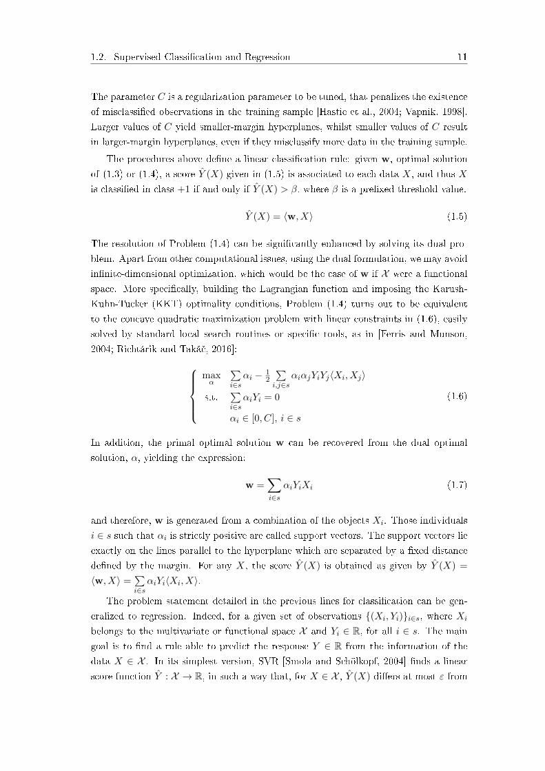
The resolution of Problem (1.4) can be signi�cantly enhanced by solving its dual pro-
blem. Apart from other computational issues, using the dual formulation, we may avoid
in�nite-dimensional optimization, which would be the case of w if X were a functional
space. More speci�cally, building the Lagrangian function and imposing the Karush-
Kuhn-Tucker (KKT) optimality conditions, Problem (1.4) turns out to be equivalent
to the concave quadratic maximization problem with linear constraints in (1.6), easily
solved by standard local search routines or speci�c tools, as in [Ferris and Munson,
2004; Richtárik and Taká£, 2016]:maxα
∑i∈s
αi − 12
∑i,j∈s
αiαjYiYj〈Xi, Xj〉
s.t.∑i∈s
αiYi = 0
αi ∈ [0, C], i ∈ s
(1.6)
In addition, the primal optimal solution w can be recovered from the dual optimal
solution, α, yielding the expression:
w =∑i∈s
αiYiXi (1.7)
and therefore, w is generated from a combination of the objects Xi. Those individuals
i ∈ s such that αi is strictly positive are called support vectors. The support vectors lie
exactly on the lines parallel to the hyperplane which are separated by a �xed distance
de�ned by the margin. For any X, the score Y (X) is obtained as given by Y (X) =
〈w, X〉 =∑i∈s
αiYi〈Xi, X〉.
The problem statement detailed in the previous lines for classi�cation can be gen-
eralized to regression. Indeed, for a given set of observations {(Xi, Yi)}i∈s, where Xi
belongs to the multivariate or functional space X and Yi ∈ R, for all i ∈ s. The main
goal is to �nd a rule able to predict the response Y ∈ R from the information of the
data X ∈ X . In its simplest version, SVR [Smola and Schölkopf, 2004] �nds a linear
score function Y : X → R, in such a way that, for X ∈ X , Y (X) di�ers at most ε from
12 Chapter 1. Introduction
the obtained response Y ∈ R. The score function Y can be expressed as
Y (X) = 〈w, X〉+ b, (1.8)
where b ∈ R, and w ∈ X are the optimal solution of the hard-margin problem in (1.9):minw,b
〈w,w〉
s.t. Yi − 〈w, Xi〉 − b ≤ ε, i ∈ s,〈w, Xi〉+ b− Yi ≤ ε, i ∈ s
(1.9)
Problem (1.9) implicitly assumes that all the pairs (Xi, Yi) are well predicted with ε
precision. This is not always the case, and some errors may be allowed. As done in
the classi�cation problem, we introduce arti�cial variables ξi, ξ∗i , yielding, for a �xed
regularization parameter C, the soft-margin problem in (1.10):min
w,b,ξ,ξ∗〈w,w〉+ C
∑i∈s
(ξi + ξ∗i )
s.t. Yi − 〈w, Xi〉 − b ≤ ε+ ξi, i ∈ s,〈w, Xi〉+ b− Yi ≤ ε+ ξ∗i , i ∈ sξi, ξ
∗i ≥ 0
(1.10)
Problem (1.10) is usually more easily solved in its dual formulation. Thanks to the
Lagrangian function and the KKT conditions, Problem (1.10) can be rewritten as a
concave maximization problem with linear contraints:maxα,α∗
−12
∑i,j∈s
(αi − α∗i )(αj − α∗j )〈Xi, Xj〉 − ε∑i∈s
(αi + α∗i ) +∑i∈s
Yi(αi − α∗i )
s.t.∑i∈s
(αi − α∗i ) = 0
αi, α∗i ∈ [0, C], i ∈ s
(1.11)
and therefore the primal variables w can be written as a linear combination of the
training objects, Xi:
w =∑i∈s
(αi − α∗i )Xi (1.12)
Along this dissertation, we consider in (1.13) an equivalent SVR dual problem, by
making the change of variables νi = αi/C and ν∗i = α∗i /C, i ∈ s:maxν,ν∗
−12
∑i,j∈s
(νi − ν∗i )(νj − ν∗j )C〈Xi, Xj〉 − ε∑i∈s
(νi + ν∗i ) +∑i∈s
Yi(νi − ν∗i )
s.t.∑i∈s
(νi − ν∗i ) = 0
νi, ν∗i ∈ [0, 1], i ∈ s
(1.13)

1.2. Supervised Classi�cation and Regression 13
1.2.3 Kernels De�nition
Section 1.2.2 was devoted to linear SVM and SVR problems. In this section, a nonlinear
extension obtained by means of the so-called kernel trick, is discussed.
Nonlinear Support Vector based problems are obtained by means of a feature map
φ : X → X which embeds the original data X in a higher-dimensional space X , con-taining an inner-product. The aim of this nonlinear map φ is to translate the original
data Xi to a space in which data are linearly separable, and therefore all the procedures
explained in Section 1.2.2 can be applied. In this way, the inner product 〈Xi, Xj〉 thatappears in the objective functions of the optimization problems (1.6) and (1.13), and also
in their corresponding score functions (1.5) and (1.8), turns out to be 〈φ(Xi), φ(Xj)〉.The explicit expressions of the higher-dimensional space X and φ are not needed, since
all the calculations are done through the inner product 〈φ(Xi), φ(Xj)〉. Hence, one canjust provide the so-called kernel function K : X×X → R, [Cristianini and Shawe-Taylor,2000; Hofmann et al., 2008; Schölkopf and Smola, 2001], de�ned by:
K(Xi, Xj) = 〈φ(Xi), φ(Xj)〉 (1.14)
and therefore, the classi�cation problem (1.6) is reformulated as follows:maxα
∑i∈s
αi − 12
∑i,j∈s
αiαjYiYjK(Xi, Xj)
s.t.∑i∈s
αiYi = 0
αi ∈ [0, C], i ∈ s,
(1.15)
yielding a nonlinear classi�cation rule: given α, optimal solution of (1.15), a score Y (X)
in (1.16) is associated with each functional data X,
Y (X) =∑i∈s
αiYiK(X,Xi), X ∈ X , (1.16)
and thus X is classi�ed in class +1 if and only Y (X) > β.
In an analogous manner, the regression problem (1.13) is rewritten in the following
way:maxν,ν∗
−12
∑i,j∈s
(νi − ν∗i )(νj − ν∗j )CK(Xi, Xj)− ε∑i∈s
(νi + ν∗i ) +∑i∈s
Yi(νi − ν∗i )
s.t.∑i∈s
(νi − ν∗i ) = 0
νi, ν∗i ∈ [0, 1], i ∈ s,
(1.17)

14 Chapter 1. Introduction
transforming the score function in (1.8) into:
Y (X) =∑i∈s
(αi − α∗i )K(Xi, X) + b, X ∈ X , (1.18)
A function must satisfy some conditions to be a kernel. More precisely, a kernel K is a
positive de�nite function with satis�es the conditions provided by the Mercer's theorem
[Mercer, 1909]. [Smola and Schölkopf, 2004] clari�es that such result just means that a
kernel function can always be written as an inner product in some feature space, and
consequently, some closure properties are derived. They include the integrals of kernels
and the positive linear combinations of kernels, applied for Multiple Kernel Learning
in [Carrizosa et al., 2014] and the references therein. Moreover, the product property
holds, i.e., if K1 and K2 are two kernels, then the function de�ned in (1.19)
K(Xi, Xj) = K1(Xi, Xj)K2(Xi, Xj) (1.19)
is also a kernel.
More closure properties and details of the proof of these results can be found in
[Shawe-Taylor et al., 2004; Smola and Schölkopf, 2004].
A wide variety of kernels, mostly in �nite-dimensional spaces, are proposed in the li-
terature. We can mention for instance the linear kernel, [Carrizosa and Romero Morales,
2013; Cristianini and Shawe-Taylor, 2000; Hofmann et al., 2008], in (1.20),
K(Xi, Xj) = 〈Xi, Xj〉 (1.20)
which will lead the simplest Support Vector problems (1.6) and (1.13).
As stated in [Vapnik, 1995], polynomial functions of type (1.21)
K(Xi, Xj) = (1 + 〈Xi, Xj〉)D (1.21)
are kernels too.
The Gaussian (RBF) kernel, de�ned with a bandwidth parameter ω in (1.22), is
the most popular kernel, mainly due to its excellent empirical behavior, [Carrizosa
et al., 2014; Cristianini and Shawe-Taylor, 2000; Keerthi and Lin, 2003]. Along this
dissertation, we will just focus on the RBF kernel, even though the applications proposed
in this thesis can be easily extended to other kernels.
K(Xi, Xj) = exp(−ω〈Xi −Xj , Xi −Xj〉) (1.22)
So far, the reasonings made through Sections 1.2.2 and 1.2.3 are valid either for �nite
or in�nite-dimensional spaces. By contrast, in the following lines, we restrict ourselves

1.2. Supervised Classi�cation and Regression 15
to the case in which the data are functional with the aim of clearly de�ne the di�erent
kernels which will be analyzed in the next chapters of the dissertation.
Formally speaking, let Xi, Xj : [0, T ]→ R belonging to the Hilbert functional space
X = F . The simplest way to deduce the functional version of the �nite-dimensional
Gaussian kernel, is just to de�ne the inner product as:
〈Xi, Xj〉 =
∫ T
0Xi(t)Xj(t)dt, Xi, Xj ∈ F (1.23)
which combined with (1.22), for a given bandwidth ω, yields:
K(Xi, Xj , ω) = exp
(−ω
∫ T
0(Xi(t)−Xj(t))
2dt
), Xi, Xj ∈ F (1.24)
When data are multivariate, i.e., X = Fp, the product property de�ned in (1.19)
will be used. Particularly, the following Gaussian kernel with a �xed bandwidth
ω = (ω1, . . . , ωp), is produced:
K(Xi, Xj ,ω) = exp
(−
p∑v=1
ωv
∫ T
0(Xiv(t)−Xjv(t))
2dt
), Xi, Xj ∈ Fp (1.25)
For hybrid functional data as in (1.2), the last p2 integral terms in (1.25) can be sub-
stituted by ordinary squared sums as follows:
K(Xi, Xj ,ω) = exp
− p1∑v=1
ωv
∫ T
0(Xiv(t)−Xjv(t))
2dt−p2∑
v=p1+1
ωv(Xiv −Xjv)2
, Xi, Xj ∈ Fp1×Rp2
(1.26)
Finally, since in practice, functional data are only measured in a �nite grid of points,
let say t = (t1, . . . , tH), the integrals of Equation (1.25) can be approximated by sums,
in which the evaluation of the functional data in the vector t is performed, yielding:
K(Xi, Xj ,ω, t) = exp
(−
p∑v=1
H∑h=1
ωv(Xiv(th)−Xjv(th))2dt
), Xi, Xj ∈ Fp (1.27)
The expressions of the kernels given by (1.24), (1.26) and (1.27) will be studied in detail
along this dissertation.
1.2.4 Performance Estimation
If the whole data set is used to train the supervised model, over�tting may appear.
See Chapter 7 of [Friedman et al., 2001b] for more details. The performance measures
may then be overoptimistic. To avoid this issue, the usual methodology is to divide the
whole data set into three independent parts, namely training, validation, and testing.

16 Chapter 1. Introduction
Particularly, the training sample is used to build a model for a �xed combination of
parameters, the validation sample is utilized to tune such parameters, and �nally, the
e�ciency of the model is estimated in the testing sample. For instance, when building
a classi�er with the SVM problem (1.6), the optimization problem is run in the same
training sample for di�erent values of C. Then, the parameter C associated to the
largest classi�cation accuracy, measured on the validation sample, is kept. Finally, the
chosen classi�er is used to estimate the accuracy on the testing sample.
Since the results obtained with the above-mentioned tool may highly depend on the
division made, it is useful to apply the so-called k-fold cross-validation method, [Kohavi,
1995]. To be more precise, k-fold cross-validation splits the whole data set into k folds.
Then, the model is trained and validated on k−1 parts, and the remaining one is used to
test the assessment. In this way, a series of k accuracy measures on the testing samples
is given. As a �nal result, the averaged accuracy on the k testing samples is proposed
as an estimate of the goodness of �t.
The number of folds k frequently depends on the cardinality of the databases. If
insu�cient data are available, then the so-called leave-one-out is applied, i.e., k coincides
with the number of observations. Therefore, the model is run each time with all the
individuals except one, which will be used to test the results.
1.3 Feature Selection
The analysis of (high-dimensional) data entails some di�culties associated with the high
computational costs, and the introduction of redundancy and noise from measurement
errors, which are usually associated with lower performance measures. Hence, to avoid
these issues, it is useful to apply feature selection strategies.
Feature selection is a key preprocessing step in data mining due to several reasons.
First, interpretability may be enhanced and monitoring costs may be reduced if just
a few number of features capable of making good predictions is considered instead of
the original and usually large set of features. Second, to select the most important
features makes sense in real-world problems, since as shown in e.g., the gene expression
work [Golub et al., 1999], the relevant information may be summarized in just some
points. Last but not least, the redundant information introduced by the original data
can be surmounted by means of feature selection tools, yielding equivalent or even better
performance values.
A plethora of works have been published on feature selection. [Blum and Langley,
1997] was one of the �rst papers published on this topic. Here feature selection was per-
formed on data sets containing approximately 40 features. The survey of [Guyon and
Elissee�, 2003] goes further and introduces several feature selection approaches with
hundreds or even thousands of variables. The overview [Fan and Lv, 2010] summa-

1.3. Feature Selection 17
rizes the most important methods from a statistical point of view, and [Chandrashekar
and Sahin, 2014] makes a survey, focusing on the di�erences of the well-known �lter,
wrapper, and embedded methods.
In classi�cation and regression for multivariate data, we should emphasize the works
[Benítez-Peña et al., 2018; Bertolazzi et al., 2016; Carrizosa et al., 2011; Maldonado and
Weber, 2009; Maldonado et al., 2011; Rakotomamonjy, 2003] in the former case, and
[Andersen and Bro, 2010; Mehmood et al., 2012; Mitchell and Beauchamp, 1988; Smith
and Kohn, 1996; Yang and Ong, 2011; Zhang, 2009] in the latter.
For functional data, di�erent perspectives have been addressed to deal with the
feature selection problem. Dimensionality reduction, for instance, is based on the pro-
jection of the functional data on lower-dimensional spaces. These include, among others,
FPCA [Górecki and Krzy±ko, 2012; Hall et al., 2001; Li et al., 2013; Lin et al., 2015;
Locantore et al., 1999], Partial Least Squares (PLS) [Aguilera et al., 2016; Delaigle
and Hall, 2012b; Preda et al., 2007; Wang and Huang, 2016], and B-splines functions
[James and Hastie, 2002; Wang et al., 2007]. For other dimensionality reduction tech-
niques in functional data, see [Ferraty and Vieu, 2002; Hsing and Ren, 2009; Li and
Hsing, 2010; Zhang et al., 2013]. It is also very common to use sparsity techniques to
handle situations in which feature selection is involved. [James et al., 2009] seeks the
non-zero ranges of the coe�cient function for a functional linear regression model, by
using a regularized least-squared method. In a non-supervised classi�cation context,
papers such as [Chamroukhi, 2016; Chamroukhi and Nguyen, 2018; Hébrail et al., 2010;
Samé et al., 2011] work with functional data with regime changes, i.e., they assume that
the functions are formed by successive shifting domains, where some of them may be
zero-weighted. A di�erent feature selection methodology in FDA is known as variable
selection. Variable selection aims to �nd a subset of relevant time instants which rep-
resent well the function, and yield acceptable performance values, as well. Regarding
functional regression, some references such as [Kneip et al., 2016; McKeague and Sen,
2010] should be highlighted. In [Kneip et al., 2016] a method is proposed to detect the
most important points of impact among a prede�ned set of time instants in which the
functional data are measured, i.e., it is assumed that the impact points only belong to
the set of timestamps where the functions are monitored, which is not always the case.
Moreover, [Kneip et al., 2016] is a generalization of the model proposed in [McKeague
and Sen, 2010] where the identi�ability and estimation of just one time instant is sought.
The work of [Aneiros and Vieu, 2014] directly applies standard multivariate procedures
to discretized functional data. Thus, the functional nature of the data is disregarded
and not exploited. The optimal selection of the time instants in functional nonparame-
tric regression models has been studied too. For example, on the works of [Aneiros and
Vieu, 2016; Ferraty et al., 2010], the most in�uential design points are sought among
a given (large) set, usually hard to obtain, while the methodologies of [Berrendero et

18 Chapter 1. Introduction
al., 2018; Ferraty et al., 2010] based on a greedy approach, in which the time instants
are sequentially located. On functional classi�cation, we should highlight for example,
[Lindquist and McKeague, 2009], where one single time instant is sought, and, as ad-
mitted in the paper, it is not possible to generalize their methodology to search for a
set of more time instants. We also emphasize the recent works of [Berrendero et al.,
2016a,b, 2017; Torrecilla and Suárez, 2016; Torrecilla Noguerales, 2015], where greedy
approaches, yielding local optima, are used. These papers follow a combinatorial ap-
proach: such time instants are assumed to belong to the �nite set of instants at which
actual measurements exist.
Unfortunately, the vast literature mentioned above is restricted on univariate func-
tional data. Feature selection methods on multivariate (hybrid) functional data have
been rarely studied. Indeed we can only make reference to some PCA-based approaches,
e.g., [Berrendero et al., 2011; Jacques and Preda, 2014] where the dimension is reduced.
1.4 Contributions of this Thesis
The goal of this thesis is to solve new Supervised Learning problems in Functional
Data by means of Mathematical Optimization tools. The functional nature of the
data is taking into account in all these models, which successfully improve the current
benchmark prediction results. This section brie�y describes the problems addressed, as
well as the challenges involved regarding the Supervised Learning �eld.
Chapter 2 is based on the work [Blanquero et al., 2017]. We address the problem of
selecting the most informative time instants in binary classi�cation with multivariate
functional data. Selecting a �nite set of time instants may lead to an improvement in the
predictive ability of the estimated model, in addition to reducing the model complexity.
Our proposal is not restricted to multivariate functional data. Indeed, our approach
allows one to classify univariate functional data in the very same way by using high-order
information of the data, e.g., monotonicity or convexity through the derivatives. The
aforementioned optimization problem is a Global Optimization problem in continuous
variables: the time instants are to be selected to maximize the correlation between the
class label and the SVM score used for classi�cation. A nested heuristic is de�ned to
enhance the algorithmic performance in which the suboptimal solution obtained in the
simplest cases is considered as the initial solution in the more di�cult models. The
e�ectiveness of the proposal is shown in univariate and multivariate data sets from the
literature.
Chapter 3 is based on the work [Blanquero et al., 2018a]. A new functional band-
width kernel is proposed to solve the SVM problem for functional data, which improves
the accuracy obtained with the usual scalar bandwidth parameter. Our approach is
able to optimally select di�erent ranges in the domain of the function according to

1.4. Contributions of this Thesis 19
their classi�cation ability. Both the kernel and the SVM parameters are tuned with
a surrogate of the accuracy, namely, the correlation between the actual class and the
SVM score. Such parameter tuning yields a continuous optimization problem, allowing
us to use gradient methods, known to be more e�cient than the optimization meth-
ods available for piecewise constant performance measures, such as the misclassi�cation
rate. Moreover, the proposed method is enhanced by de�ning a hierarchy of kernel
bandwidths models of increasing complexity, inspired by the nested model previously
proposed for Multiple Kernel Learning. By using this hierarchy will provide wide �e-
xibility since complex parameterizations of the functional bandwidth can be e�ciently
optimized from more simple ones. Our experiments with benchmark data sets show the
advantages of using functional parameters and the e�ectiveness of our approach.
Chapter 4 is based on the work [Jiménez-Cordero and Maldonado, 2018], where a
feature selection problem for hybrid functional data is treated. Our aim is to select the
most important covariates, either functional or static, in order to achieve good classi-
�cation predictions. In this chapter, an embedded feature selection approach for SVM
classi�cation is proposed, where the isotropic Gaussian kernel is modi�ed by associating
a bandwidth to each feature, which automatically weighs the importance of the di�erent
variables (functional or static). The bandwidths are jointly optimized with the SVM
parameters, yielding an alternating optimization approach. The drastic improvements
in the classi�cation rates, as well as the robustness of our methodology, were tested on
benchmark data sets.
The results provided in Chapter 2 can be extended to regression. In fact, Chapter 5,
based on [Blanquero et al., 2018b], outlines the problem of selecting a small set of time
instants able to capture the information needed to predict a scalar response variable
from multivariate functional data. More precisely, selecting from the full monitoring
interval a few time instants without damaging prediction accuracy would de�nitely lead
to a much better understanding of the data, enhancing quicker predictions and easing
decision making. Replacing the whole interval by a low-dimensional vector of time
instants can be seen as a variable selection procedure from an in�nite set of features.
The regression tool used in this chapter is SVR, and a continuous optimization algorithm
is proposed to �t the parameters and select the time instants as well. We illustrate the
usefulness of our proposal in some benchmark data sets.


Chapter 2
Variable Selection in Functional
Data Classi�cation with SVM
21

2.1. Introduction 23
2.1 Introduction
Functional data classi�cation entails some di�culties associated with the high compu-
tational costs, and the introduction of redundancy and noise from measurement errors,
which may deteriorate the correct classi�cation performance. Since functional data
are intrinsically in�nite-dimensional data, it is thus useful to select the time instants
providing the most relevant information of the data, i.e., to perform variable selection.
In this chapter, we address the problem of classifying multivariate functional data
into two pre�xed classes by using the information provided by a training sample. More
precisely, our goal is to select the most informative time instants in order to obtain good
classi�cation rates. Classi�ers will be based on the benchmark supervised classi�cation
tool SVM, detailed in Section 1.2.2.
Variable selection for multivariate functional data has been scarcely analyzed in
the literature yet, as Section 1.3 outlines. Therefore, the main contribution of this
chapter is to provide a new strategy able to �nd the most informative time instants
to achieve good classi�cation rates in multivariate functional data. Contrary to the
usual trend in the literature, [Berrendero et al., 2016a,b, 2017; Torrecilla and Suárez,
2016; Torrecilla Noguerales, 2015], we consider the time as a continuous variable, and
we search for an optimal SVM-classi�er using a surrogate of the rate of misclassi�ed
data, namely the correlation between the SVM score and the actual class. Finding such
optimal time instants amounts to solving a continuous smooth optimization problem.
Moreover, our algorithmic strategy is improved thanks to the de�nition of nested models
of increasing complexity, following the idea in [Carrizosa et al., 2014].
Finally, our framework can accommodate from one to several functions, allowing
one to address in the very same way univariate and multivariate functional data. In
particular, one can easily include in the model higher-order information (monotonicity,
convexity, ...) by replacing each univariate functional datum by a multivariate one, cor-
responding to the functional datum itself and its derivatives. The information provided
by the derivatives has been utilized in the clustering context, [Ieva et al., 2013; Meng
et al., 2018], with outstanding results.
The remainder of this chapter is structured as follows. In Section 2.2 we present the
variable selection problem, including the management of the functional data derivatives.
In addition, the problem formulation, as well as the solving strategy are detailed. Section
2.3 is focused on the numerical experiments, and �nally Section 2.4 presents some
conclusions and extensions.
24 Chapter 2. Variable Selection in Functional Data Classi�cation with SVM
2.2 A Global Optimization Approach to the Variable Se-
lection Problem
In this section, the mathematical formulation of the variable selection problem in SVM
classi�cation with functional data is outlined. Section 2.2.1 brie�y presents the variable
selection problem and details how the higher-order information can be included in the
multivariate data structure. Section 2.2.2 is devoted to the problem formulation and
the solving strategy, whereas a nested heuristic is proposed in Section 2.2.3, in which
we take advantage of the fact that the di�erent time instants t = (t1, . . . , tH) can be
easily embedded in a nested structure of models. Section 2.2.4 addresses the problem
of determining the number H of time instants.
2.2.1 Variable Selection with Functional SVM
We assume given a sample s of individuals, where each instance i ∈ s is associated
with the pair (Xi, Yi). The datum Xi ∈ X = Fp is composed by p functional features,
i.e., Xi = (Xi1(t), . . . , Xip(t)), as sketched in (1.1). The functional space F represents
the class of d−times continuously di�erentiable functions on the time interval [0, T ].
Furthermore, Yi ∈ {−1,+1} denotes the class label of the observation i ∈ s. Our aim
is to �nd a classi�cation rule which allows us to infer the class Y of a new functional
observation X ∈ X . To do this, an SVM-classi�er, obtained from the resolution of
Problem (1.15) will be used. Since our objective is to select the �nite set of H time
instants that provide the most relevant information for discriminating between two
groups, the functional kernel given in (1.27) was chosen. Hence, two types of parameters
need to be tuned: the vector of time instants, t = (t1, . . . , tH), such that
0 ≤ t1 ≤ . . . ≤ tH ≤ T (2.1)
and the parameters associated with the SVM problem (1.15), i.e., the regularization
parameter C and the bandwidth ω of the kernel (1.27). Extra constraints over the
parameters can be easily incorporated into the optimization problem, such as imposing
a �xed separation between the time instants. Details about the resulting optimization
problem and the solving strategy are given in Section 2.2.2.
It is worth mentioning that our methodology is not only restricted to pure multi-
variate functional data. Indeed, the approach here proposed can be directly applied to
univariate functional data, X(t) ∈ F . More speci�cally, apart from the straightforward
case in which one just considers p = 1, a preprocessing stage can be carried out in
order to transform the univariate data into multivariate ones by taking advantage of
the higher-order information throughout the usage of the derivatives of X. This process

2.2. A Global Optimization Approach to the Variable Selection Problem 25
yields data of the form:
(X(t), X ′(t), . . . , Xd)(t)), (2.2)
where Xd)(t) denotes the d−th derivative of X(t). Moreover, the information provided
by the derivatives can also be added to the pure multivariate functional case, yielding
(X1(t), . . . , Xp(t), X′1(t), . . . , X ′p(t), . . . , X
d)1 (t), . . . , Xd)
p (t)). (2.3)
The numerical experience in Section 2.3 shows that the higher-order information will
be crucial in the classi�er performance.
We also recall that, in practice, the original functional data Xi may be only available
throughout a grid of time instants. Therefore, interpolation techniques, such as cubic
splines, [De Boor, 1978; Friedman et al., 2001b], should be used as a preprocessing step
so that the functional data can be properly rebuilt. It is important to remark that the
interpolation step recovers the smoothness of the data with respect to t.
Furthermore, if we want to take advantage of the higher-order information of the
data, it is necessary to get, as preprocessing, the derivatives from the data X(t). One
possible choice would be to compute the derivatives of the smoothed data. Nevertheless,
in order to avoid the propagation of numerical errors from the interpolation, we suggest
using the �nite-increments as an approximation of the derivatives. For instance, the
�rst derivative of X(t) in a point th admits the following approximation:
X ′(th) =X(th)−X(th−1)
th − th−1(2.4)
Note that in (2.4), th, ∀h, indicate the time instants where the functional data are
discretized. The formula in (2.4) should be reproduced for all the time points of the
discretization, and extended to any derivative's order. After obtaining the discretized
derivatives, they should be smoothed with an interpolation technique, as explained
before.
2.2.2 The Bilevel Optimization Problem
As previously mentioned, two di�erent types of decision variables are involved in the
variable selection problem for classi�cation of functional data with SVM. First, the H
time instants t = (t1, . . . , tH) satisfying (2.1), and second, the parameters C and ω
involved in the SVM problem (1.15), and in the Gaussian kernel (1.27), respectively.
Di�erent strategies are proposed here to �nd the optimal values of C,ω and t. C is
obtained by using a standard grid search, while a bilevel optimization problem is de�ned
to tune the parameters ω and t. In such bilevel problem we propose to maximize the
Pearson correlation coe�cient between the class label Yi of the observation i ∈ s, andthe score Y (Xi(t),ω, α) in (1.16). Other references in the literature, such as [Székely et

26 Chapter 2. Variable Selection in Functional Data Classi�cation with SVM
al., 2007; Torrecilla Noguerales, 2015], have previously used similar performance mea-
sures, with excellent results. Despite the fact that, when using the Pearson correlation
coe�cient as a surrogate of accuracy, a linear relationship between the binary label,
Y ∈ {−1,+1}, and the real-valued score, Y ∈ R, is implicitly assumed, such coe�cient
is very fast to compute and even more important, it yields a smooth optimization pro-
blem, in which gradient information can be used to speed up the convergence. This last
issue means a signi�cant advantage over the use of other performance measures, such as
those based on the confusion matrix, which usually lead to mixed-integer optimization
problems hard to solve for realistic data sizes.
In this chapter, the parameters and time instants sought, as well as the performance
estimates of the classi�er, are obtained as follows: the database is split into k folds, as
detailed in Section 1.2.4. Then, k − 1 folds are chosen to be again divided into three
parts, yielding the samples s1, s2 and s3. Finally, the remaining fold constitutes the
fourth independent sample s4. Samples s1 and s2 act as training samples, while s3 and
s4 are the validation and testing samples, respectively. This division process is repeated
one time per fold.
Regarding the role of each sample in the optimization strategy, sample s1 is used to
obtain the SVM dual variables, α, solving Problem (1.15) for �xed ω, t and C. Sample
s2 is employed to compute R((Yi, Y (Xi(t,ω, α)))i∈s2), i.e., the correlation coe�cient
between the class labels and the scores de�ned in (1.16). Sample s3 is used to tune
the regularization parameter C, by evaluating the accuracy for all the values of C in a
grid, and keeping the one with the largest value. Finally, the accuracy obtained with
the optimal parameters is estimated on the independent sample s4.
To sum up, for a �xed C, the resulting bilevel optimization problem is given in (2.5)
maxα,ω, t
R((Yi, Y (Xi(t),ω, α))i∈s2)
s.t. α solves (1.15) in s1,
ωv ≥ 0, v = 1, . . . , p
0 ≤ t1 ≤ . . . ≤ tH ≤ T
(2.5)
Note also that we have emphasized the dependence of the score Y on the time
instants in t, on the bandwidth ω, and on the classi�cation coe�cients α in the notation.
When such values are clear, they will be omitted in the notation for the sake of simplicity.
Problem (2.5) is a nonlinear problem which can be solved with the techniques des-
cribed in e.g., [Colson et al., 2007]. For instance, we may mention branch-and-bound
schemes in which the problem is reformulated under some convexity assumptions using
the KKT conditions. Even with these reductions, the so-obtained problem is di�cult
to solve due to the nonconvexities in the complementary and Lagrangian constraints.
Penalty function methods can also be used to solve bilevel problems, but convergence

2.2. A Global Optimization Approach to the Variable Selection Problem 27
is to stationary points.
Instead of the above-mentioned resolution methods, we propose to address the bilevel
problem (2.5) for each C by a procedure consisting in two alternating steps: the SVM
step, in which for ω and t �xed, we solve Problem (1.15) to obtain the optimal SVM
variables α; and the max-corr step, where for α �xed, one maximizes the Pearson
correlation coe�cient R in (2.6) to obtain the optimal bandwidth ω and the time
instants t. This correlation maximization problem can be expressed as:maxω,t
R((Yi, Y (Xi(t),ω))i∈s2)
s.t. ωv ≥ 0, v = 1, . . . , p
0 ≤ t1 ≤ . . . ≤ tH ≤ T
(2.6)
Di�erent strategies are used to solve Problems (1.15) and (2.6). The standard local
search routines, speci�ed in Section 1.2.2, can be applied for the SVM Problem (1.15).
On the other hand, Problem (2.6) is a continuous optimization problem, where classic
local searches are combined with a multi-start approach to avoid getting stuck at local
optima. The initial values of ω and t in the �rst iteration of the alternating approach
are randomly selected in their corresponding domains of de�nition.
The alternating procedure is run until some stopping criteria, such as the number of
evaluations or the maximum time allowed is reached, yielding certain values of ω, t and
α, for a �xed C. The value of C is chosen by applying a grid search, i.e., for each value
of C in a grid, the accuracy obtained with the classi�cation rule obtained after solving
Problem (2.5), is measured in sample s3. The parameter C with the best accuracy will
be kept. Finally, we test our approach by measuring the accuracy in a fourth sample,
s4.
Calculating the gradient of the objective function in (2.6) will reduce the compu-
tational e�ort, since numerical di�erentiation is avoided. Just applying the chain rule
and taking into account (2.7), i.e., the derivative of the kernel function in (1.27) with
respect to the parameters in ω and t, we can easily obtain an explicit expression for
the gradient of the objective function in (2.6):
∂K(Xi, Xj ,ω, t)
∂ωv= K(Xi, Xj ,ω, t)
− H∑h=1
(Xiv(th)−Xjv(th))2
v = 1, . . . , p
∂K(Xi, Xj ,ω, t)
∂th= −2K(Xi, Xj ,ω, t)
p∑v=1
(ωv(Xiv(th)−Xjv(th)))×
×(∂Xiv(t)
∂t
∣∣∣t=th− ∂Xjv(t)
∂t
∣∣∣t=th
), h = 1, . . . ,H (2.7)
The pseudocode of our approach is outlined in Algorithm 1, and an extension of it

28 Chapter 2. Variable Selection in Functional Data Classi�cation with SVM
based on a nested heuristic is detailed in Section 2.2.3.
Algorithm 1 Heuristic for variable selection
Input: H• Randomly split the sample s into s1, s2, s3 and s4.• Compute the derivatives of the functional data.• Smooth the data with some interpolation technique.for C in the grid do
Alternating Procedurerepeat
1. Fixed ω, t, calculate the parameters α of the SVM clasi�er bysolving Problem (1.15) using s1.
2. Fixed α, compute ω, t by solving Problem (2.6) over s2.until stopping criteria• Evaluate the accuracy using the sample s3 for the C �xed in the grid.
end for• The optimal value of C is the one with best accuracy in s3, and the optimal valuesof α, ω and t are the parameters associated to the optimal C.Output: Optimal parameters ω, t, C, α, and the accuracy estimated from s4.
2.2.3 A Nested Heuristic
In this section we enhance the basic heuristic detailed in Algorithm 1. Adopting the idea
of [Carrizosa et al., 2014], we propose to de�ne a series of nested models of increasing
complexity, where the optimal solution of the elementary case is used as a starting
solution in the following more complex model.
The idea is that, in order to �nd the vector th+1 of h+1 time instants, one can use as
starting solution a perturbation of th, the solution obtained when only h time instants
are sought. Therefore, if we want to �nd the H time instants which best discriminate
between two groups, we apply successively the Alternating Procedure of Algorithm 1
for h = 1 to H, but considering the easy-to-tune structure of the simple models as
a simpli�cation of the complex cases, in such a way that the (suboptimal) solution
K(Xi, Xj ,ωh, th) is used as an initial solution for kernel K(Xi, Xj ,ω
h+1, th+1). More
precisely, in order to build the initial solution for the h+1 time instants in th+1, we �rst
select a random value τ ∈ [0, T ], and then we include it in the appropriate position of
the optimal solution of the level h, thopt, in such a way that th+1 satis�es the conditions
in (2.1), i.e., th+1 := σ(τ, thopt), where σ is the function that sorts in increasing order
the time instants thopt and τ .
One of the advantages of our nested heuristic is that it allows us to obtain a trajec-
tory of the accuracy in terms of the number of time instants chosen. This is a crucial
issue, since, in practice, the numberH of time instants to consider may not be �xed, and
thus a list of classi�ers, with di�erent complexity (H) and accuracy, can be provided.

2.2. A Global Optimization Approach to the Variable Selection Problem 29
Note that the solution of the level h will be used just as a starting point of level h+1,
in order to speed up the algorithm, but still allows the algorithm to yield a solution
that is very di�erent from the level h solution. In this way, our proposal clearly di�ers
from [Torrecilla Noguerales, 2015], where greedy schemes are proposed.
The pseudocode of the nested heuristic is shown in Algorithm 2.
Algorithm 2 Nested heuristic for variable selection
Input: H, nested kernels K(Xi, Xj ,ω1, t1) ≺ . . . ≺ KH(Xi, Xj ,ω
H , tH).• Randomly split the sample s into s1, s2, s3 and s4.• Compute the derivatives of the functional data.• Smooth the data with some interpolation technique.for C in the grid do
Initialization:• h := 1.• Randomly select an initial solution ω1 ∈ [0,+∞)p and t1 := t1 ∈ [0, T ].• Set (ω, t) := (ω1, t1).while h ≤ H do
1. Run the Alternating Procedure of Algorithm 1 forK(Xi, Xj ,ω
h, th), starting from (ω, t) and yielding (ωhopt, thopt) as
solution, using samples s1 and s2.2. Randomly generate τ ∈ [0, T ].3. Set ωh+1 := ωhopt, t
h+1 := σ(τ, thopt), (ω, t) := (ωh+1, th+1) andh := h+ 1.
4. Evaluate the accuracy over the sample s3 with C �xed.end while
end for• For h �xed, the optimal value of C is the one with the best accuracy in s3. Theoptimal values of α, ω and t are the parameters associated to the optimal C.Output: Optimal parameters ωhopt, t
hopt, ∀h, the associated coe�cients C,α, and the
accuracy estimated from s4.
2.2.4 Choice of the Number of Variables, H
The choice of the optimal number of time instants, H, is a critical issue. The larger is
H, the better is the classi�cation accuracy expected to be obtained, although the risk of
over�tting increases. However, the smaller the value of H, the easier the interpretation
of the results obtained.
In this chapter, we propose to follow the common strategy carried out in the litera-
ture, [Berrendero et al., 2016a,b, 2017; Torrecilla and Suárez, 2016; Torrecilla Noguerales,
2015], and choose the value of H by estimating the accuracy on the validation sample
s3 with k−fold cross-validation. The value of H with the largest accuracy will be kept.

30 Chapter 2. Variable Selection in Functional Data Classi�cation with SVM
2.3 Numerical Experiments
This section details the computational results of our approach, in which we provide the
accuracy obtained when only some selected time instants, instead of the whole functional
interval [0, T ], are considered. Section 2.3.1 describes the settings of the computational
experience, and in Section 2.3.2 the description of the data sets is given. The results
obtained for the di�erent databases are presented in Section 2.3.3.
2.3.1 Description of the Experiments
Our proposal has been applied to both univariate and multivariate functional data. On
top of comparing the performance of the SVM based on the full time interval against
the SVM classi�er for data measured at just H time instants, we have also analyzed the
improvements in performance obtained when, instead of the functional data alone, up
to d derivatives of the functional data are also included in the input. For this reason,
we have also run Algorithm 2 for three di�erent values of d, namely d = 0, 1, 2, which
correspond respectively to the cases in which just the information of the functional data,
or also its monotonicity, or both monotonicity and convexity, are considered.
In order to obtain stable results, k−fold cross-validation is performed. The number
of folds, k, will be 10 in the databases with more than 100 individuals, or it will
coincide with the number of individuals of the database in the remaining data sets.
The cardinality of each database is shown in Table 2.1. Algorithm 2 is run k times,
one per fold. Each time, the data set is divided into four samples s1 − s4 as explained
in Section 2.2.2. To test our results we provide the average of the accuracy across the
folds, measured on s4. The number of iterations of the multi-start is �ve, the number
of iterations of the Alternating Procedure in Algorithm 1 is ten, and the (maximum)
number of time instants to be selected, i.e., the number of nested kernels, is H = 19.
Finally, the parameter C takes values in the set {2−10, . . . , 210} in logarithmic scale.
Apart from the experiments explained above, we have also tuned the optimal number
of time instants, H by performing cross-validation on sample s3, as explained in Section
2.2.4.
The whole computational experience is executed on a cluster with 2 terabytes of
RAM memory at 6.2 TFlops, running CentOS Linux 7.3, and it is coded in R, [Core
Team, 2017].
2.3.2 Description of the Data Sets
Three univariate (growth, phoneme_large and tecator) and three multivariate (batch,
batch_noise and trigonometric) functional databases have been considered to check the
performance of our approach. Samples of ten individuals of each data set are plotted
in Figure 2.1 (univariate data) and 2.2 (multivariate data). The records in class −1

2.3. Numerical Experiments 31
are depicted with a solid blue line, whereas the records in class +1 are plotted in red
dashed line.
Table 2.1 shows the number of records of each database, the number of time instants
in which the records are measured, the number of records of each class and the number
of components of the functional data vector. A detailed description of each database
follows.
#records #time instants #records label -1 #records label +1 #components
growth 93 31 54 39 1phoneme_large 1717 256 1022 695 1
tecator 215 100 77 138 1batch 100 101 50 50 3
batch_noise 100 101 50 50 3trigonometric 400 1001 200 200 2
Table 2.1: Data description summary
Growth Data Set
This data set was �rst introduced in [Tuddenham and Snyder, 1954], and has been
studied in several works, e.g., [Cuevas et al., 2007; Muñoz and González, 2010; Tor-
recilla Noguerales, 2015]. It is available in the fda library of R. The data set contains
the height in centimeters of an amount of 93 individuals ranging from the age of 1 to 18
years measured on 31 non-equally spaced time instants. More speci�cally, the heights
of 39 boys and 54 girls are given. The aim is to determine if a new individual is a boy
or a girl, just with the information provided by the height curve.
Phoneme_large Data Set
This database was originally presented in [Hastie et al., 1995] and can be obtained from
[Friedman et al., 2001a]. The original data set contains 4509 functions with the log-
periodograms, monitored at 256 equally spaced points, of individuals pronouncing the
following �ve phonemes: �sh� as in �she�, �dcl� as in �dark�, �iy� as the vowel in �she�, �aa�
as the vowel in �dark�, and �ao� as the �rst vowel in �water�. The �ve-class classi�cation
problem has been adapted to our binary classi�cation framework as done in [Delaigle
and Hall, 2012a; Torrecilla Noguerales, 2015], yielding a total of 1717 observations, 1022
from the phoneme �ao� and 695 from �aa�. Therefore, the goal is to build a classi�cation
rule, which di�erentiates both phonemes. Apart from the papers just cited, this data
set has also been applied in [Berrendero et al., 2016c; Friedman et al., 2001b] among
others.

32 Chapter 2. Variable Selection in Functional Data Classi�cation with SVM
Tecator Data Set
This data set deals with the near-infrared absorbance spectra of 215 samples of �nely
chopped pork, recorded at 100 equally spaced points from 850 to 1050 nanometers. It
has associated the values of the fat content, and according to [Ferraty and Vieu, 2006],
the database can be divided into two classes depending if the fat content is smaller or
larger than 20%. Moreover, the curves of tecator are usually smoothed, e.g.: [Ferraty
and Vieu, 2006; Porro et al., 2009; Torrecilla Noguerales, 2015], in order to work with
the second derivatives instead of the raw data. This reduction is also made in this
dissertation. The data can be obtained from the fda.usc library of R, and have been
analyzed in works such as [Martín-Barragán et al., 2014; Rossi and Villa, 2006].
Batch Data Set
This is a synthetic data set. The three covariates of this �rst multivariate data set,
batch, come from Section 4.1 of [Wang and Yao, 2015]. In this data set, each instance is
described by three functions Xv, v = 1, 2, 3 with very di�erent shapes: linear, quadratic
and sinusoidal, respectively. Although Wang and Yao consider that the upper bound for
the time interval in which the functions are measured follows an uniform distribution
on [0.9, 1.1], we assume, for the sake of simplicity, that Xv : [0, 1] → R, v = 1, 2, 3.
Formally:
Xi1(t) = ai · t+ γi(t)
Xi2(t) = ai · t2 + γi(t)
Xi3(t) = bi (4 sin(t) + 0.5 sin(ν0 · t)) (2.8)
for t ∈ [0, 1], where each (ai, bi) follows a bivariate Gaussian distribution with mean
vector (2.5, 2.5) and covariance matrix diag(2.5, 2.5).
For each t ∈ [0, 1], the measurements errors γi(t) are i.i.d. Gaussian noise with mean
0 and standard deviation 0.2. The individuals Xi with label Yi = +1 have ν0 = 10,
whereas those with Yi = −1 are associated with ν0 = 11.
Batch_noise Data Set
This multivariate synthetic data set comes from Section 4.2 of [Wang and Yao, 2015]
and the three covariates have the same structure as in (2.8). In this case, the coe�-
cients (ai, bi) still follows a bivariate Gaussian distribution with mean vector (2.5, 2.5)
and covariance matrix diag(2.5, 2.5). Nevertheless, the parameter ν0 = 10 for all the
individuals, and the standard deviation of the Gaussian noise γi(t) is equal to 0.2 in the
individuals with label Yi = +1, and equal to 0.3 in the observations with Yi = −1.

2.3. Numerical Experiments 33
5 10 15
8010
012
014
016
018
0
Age
Hei
ght
BoysGirls
(a) growth
0 50 100 150 200 250
−5
05
1015
2025
Time
Log−
perio
dogr
ams
aoaa
(b) phoneme
850 900 950 1000 1050−0.
003
−0.
001
0.00
00.
001
0.00
20.
003
Wavelength
Abs
orba
nce
Spe
ctra
≤ 20% fat> 20% fat
(c) tecator
Figure 2.1: Sample of functional data in the univariate data sets analyzed
Trigonometric Data Set
The trigonometric database is a synthetic data set formed by two functional features.
Functional components Xiv : [1, 21] −→ R, v = 1, 2 are based on the data generated in
34 Chapter 2. Variable Selection in Functional Data Classi�cation with SVM
Section 5.2.2 of [Jacques and Preda, 2014] and have the form:
Xi1(t) = −21
2+ t+ ν0U1 cos
(ν0
t
10
)+ ν0U1 sin
(ν0 +
t
10
)+ γi(t)
Xi2(t) = −21
2+ t+ ν0U1 sin
(ν0
t
10
)+ ν0U2 cos
(ν0 +
t
10
)+ ν0U3
((t
10
)2
+t
10+ 1
)+ γi(t)
(2.9)
where t ∈ [1, 21], U1, U2, U3 ∼ N (1, 1) are independent Gaussian variables and γi(t)
is a white noise of unit variance. The value of ν0 is dependent on the class label.
More speci�cally, the individuals with label Yi = 1 have ν0 = 1, while the observations
corresponding to Yi = −1 have ν0 = 2.
Note that the trigonometric data set is used in [Jacques and Preda, 2014] for clus-
tering purposes with three and �ve groups. Nevertheless, in this chapter, since binary
classi�cation is studied, we only consider two groups.
2.3.3 Results
In this section, we detail the computational results obtained on the univariate and mul-
tivariate functional data described in Section 2.3.2. Moreover, we present the numerical
experience for the optimal choice of the number of time instants to be considered, H.
Results on Univariate Functional Data
Table 2.2 reports the average accuracy on the testing sample of the data sets growth,
phoneme_large and tecator provided by Algorithm 2 with the information given by the
raw data (d = 0), the �rst derivative (d = 1), and the �rst two derivatives (d = 2).
Leave-one-out is performed on the growth data set, whereas 10−fold cross-validation is
done in phoneme_large and tecator. Our results are compared with acc max and acc
min, respectively the best and worst accuracy results obtained with the state-of-the-art
methods, as reported in Tables 2 and 3 of [Berrendero et al., 2016c].
Information shown in Table 2.2 is also depicted in Figure 2.3. Particularly, the
solid red-circled, blue-triangled and green-crossed lines indicates the average accuracy
obtained with d = 0, 1, 2, respectively. The horizontal black solid line and pink dashed
lines give the values of acc max and acc min, respectively.
Two main conclusions are obtained from our analysis. First, our results are compet-
itive against the state-of-the-art. Moreover, the use of higher-order information deeply
a�ects the classi�cation performance. This fact is extremely noticeable in the tecator
data set. Furthermore, in such database we are very close to the value acc max with
just H = 2 time instants and d = 2. If we focus on the growth data set, we realize that
with H = 3, 5, 10, 13, 14, and d = 2 we achieve the same accuracy as the value acc max.
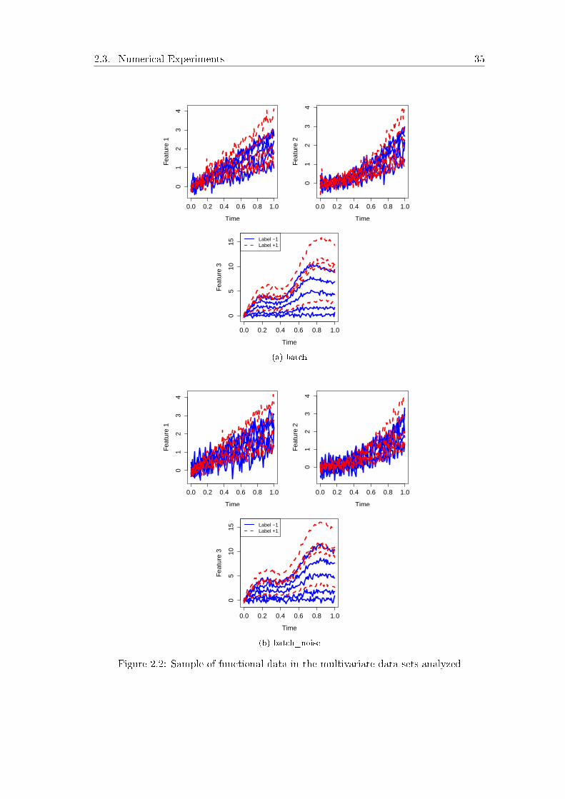
2.3. Numerical Experiments 35
0.0 0.2 0.4 0.6 0.8 1.0
01
23
4
Time
Fea
ture
1
0.0 0.2 0.4 0.6 0.8 1.0
01
23
4
Time
Fea
ture
2
0.0 0.2 0.4 0.6 0.8 1.0
05
1015
Time
Fea
ture
3
Label −1Label +1
(a) batch
0.0 0.2 0.4 0.6 0.8 1.0
01
23
4
Time
Fea
ture
1
0.0 0.2 0.4 0.6 0.8 1.0
01
23
4
Time
Fea
ture
2
0.0 0.2 0.4 0.6 0.8 1.0
05
1015
Time
Fea
ture
3
Label −1Label +1
(b) batch_noise
Figure 2.2: Sample of functional data in the multivariate data sets analyzed
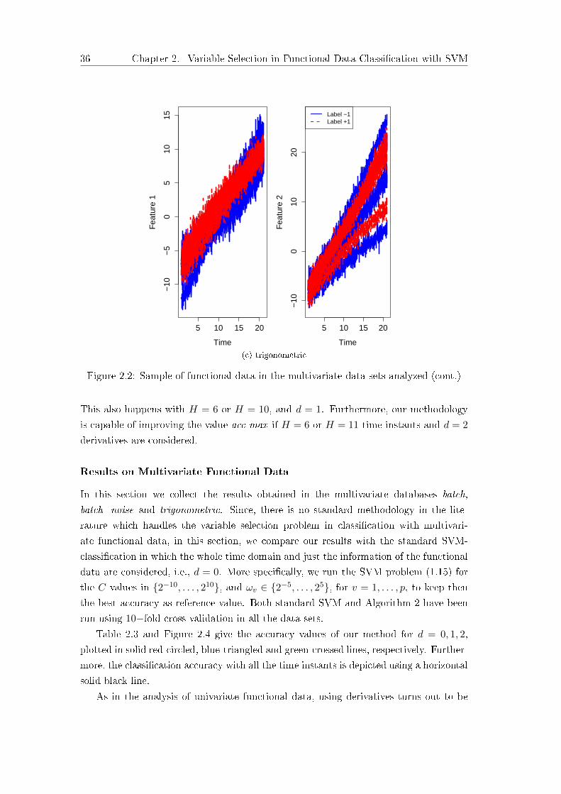
36 Chapter 2. Variable Selection in Functional Data Classi�cation with SVM
5 10 15 20
−10
−5
05
1015
Time
Fea
ture
1
5 10 15 20
−10
010
20
Time
Fea
ture
2
Label −1Label +1
(c) trigonometric
Figure 2.2: Sample of functional data in the multivariate data sets analyzed (cont.)
This also happens with H = 6 or H = 10, and d = 1. Furthermore, our methodology
is capable of improving the value acc max if H = 6 or H = 11 time instants and d = 2
derivatives are considered.
Results on Multivariate Functional Data
In this section we collect the results obtained in the multivariate databases batch,
batch_noise and trigonometric. Since, there is no standard methodology in the lite-
rature which handles the variable selection problem in classi�cation with multivari-
ate functional data, in this section, we compare our results with the standard SVM-
classi�cation in which the whole time domain and just the information of the functional
data are considered, i.e., d = 0. More speci�cally, we run the SVM problem (1.15) for
the C values in {2−10, . . . , 210}, and ωv ∈ {2−5, . . . , 25}, for v = 1, . . . , p, to keep then
the best accuracy as reference value. Both standard SVM and Algorithm 2 have been
run using 10−fold cross-validation in all the data sets.
Table 2.3 and Figure 2.4 give the accuracy values of our method for d = 0, 1, 2,
plotted in solid red-circled, blue-triangled and green-crossed lines, respectively. Further-
more, the classi�cation accuracy with all the time instants is depicted using a horizontal
solid black line.
As in the analysis of univariate functional data, using derivatives turns out to be
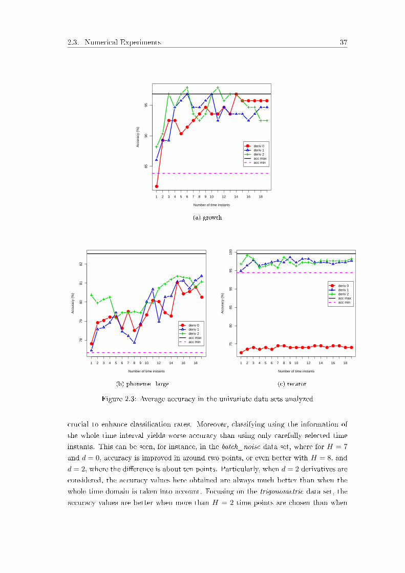
2.3. Numerical Experiments 37
●
●
● ●
●
●
●
●
●
● ●
●
●
●
● ● ● ● ●
8590
95
Number of time instants
Acc
urac
y (%
)
1 2 3 4 5 6 7 8 9 10 12 14 16 18
● deriv 0deriv 1deriv 2acc max acc min
(a) growth
●
●●
● ●
●
●
●
●
●
●●
●
●
●
●●
●
●
7879
8081
82
Number of time instants
Acc
urac
y (%
)
1 2 3 4 5 6 7 8 9 10 12 14 16 18
● deriv 0deriv 1deriv 2acc max acc min
(b) phoneme_large
●
●●
●●
●
● ●● ● ● ●
● ●●
● ●● ●
7580
8590
9510
0
Number of time instants
Acc
urac
y (%
)
1 2 3 4 5 6 7 8 9 10 12 14 16 18
● deriv 0deriv 1deriv 2acc max acc min
(c) tecator
Figure 2.3: Average accuracy in the univariate data sets analyzed
crucial to enhance classi�cation rates. Moreover, classifying using the information of
the whole time interval yields worse accuracy than using only carefully selected time
instants. This can be seen, for instance, in the batch_noise data set, where for H = 7
and d = 0, accuracy is improved in around two points, or even better with H = 8, and
d = 2, where the di�erence is about ten points. Particularly, when d = 2 derivatives are
considered, the accuracy values here obtained are always much better than when the
whole time domain is taken into account. Focusing on the trigonometric data set, the
accuracy values are better when more than H = 2 time points are chosen than when

38 Chapter 2. Variable Selection in Functional Data Classi�cation with SVM
the whole time interval is considered.
●
●
●
●
●
●
●
●
●
●
●
●
●
●
●
●
● ●
●
5 10 15
6570
7580
8590
Number of time instants
Acc
urac
y (%
)
1 2 3 4 5 6 7 8 9 10 12 14 16 18
● deriv 0deriv 1deriv 2whole time domain
(a) batch
●
●
●
●
●
●
●
●
●
●
●
●
● ●
●
●
●
●
●
5 10 15
6065
7075
80
Number of time instants
Acc
urac
y (%
)
1 2 3 4 5 6 7 8 9 10 12 14 16 18
● deriv 0deriv 1deriv 2whole time domain
(b) batch_noise
●
● ●
●
●
●
●
●
●
●
● ● ●
●
●
●
●
●
●
5 10 15
9294
9698
Number of time instants
Acc
urac
y (%
)
1 2 3 4 5 6 7 8 9 10 12 14 16 18
● deriv 0deriv 1deriv 2whole time domain
(c) trigonometric
Figure 2.4: Average accuracy in the multivariate data sets analyzed
Results on the optimal choice of the time instants, H
In order to obtain the best number of time instants, H, we performed cross-validation
on the validation sample s3, as detailed in Section 2.2.4. Table 2.4 shows the average
optimal number of time instants over all the folds in the univariate and multivariate
databases when H is varied. Moreover, in Figures 2.5 and 2.6 the resulting boxplots
2.4. Conclusions and Extensions 39
are depicted. In the x−axis, the maximum number of time instants considered when
running our heuristic is given, whereas the y−axis indicates the optimal number of time
instants obtained across the di�erent runs. Boxplots in red, blue and green show the
results when the information of the derivative d = 0, d = 1 or d = 2 is used, respectively.
We can observe that, although the experiments are run until H = 19, the optimal
number of time instants to be selected is lower in almost all databases. Indeed, most of
the data sets need between 1 and 8 time instants. It implies that data information is
summarized on a small �nite set of time points, which may improve the interpretability
of the results.
2.4 Conclusions and Extensions
We have proposed in this chapter a new approach to optimally select the most infor-
mative time instants in multivariate functional data classi�cation. Furthermore, our
methodology, by its nature, allows the easy usage of high-order information, e.g., mono-
tonicity, or convexity by means of the derivatives. The numerical experience reported
has shown that the information provided by the derivatives has valuable consequences in
the classi�cation performance, yielding competitive results when are compared against
the state-of-the-art in the literature. We have worked under the assumption that time
is a continuous parameter, and continuous optimization tools are then used to achieve
an optimal choice of the parameters.
The nested structure of the problem is exploited to enhance running times by using
the optimal solutions obtained in simpler models as starting solutions in more complex
models.
In our analysis, for the sake of simplicity, we have considered the Pearson cor-
relation coe�cient as the performance measure to be optimized. Nevertheless, other
measurements such as the Mutual Information Criterion [Cover and Thomas, 2006;
Gómez-Verdejo et al., 2009], the Fisher-Correlation Criteria, [Ding and Peng, 2005], the
distance covariance [Berrendero et al., 2016b; Székely et al., 2007; Torrecilla Noguerales,
2015], or the distance correlation in [Torrecilla Noguerales, 2015] can be used.
We have restricted ourselves to the pure multivariate functional data case. The pro-
blem of time instants selection in multivariate hybrid functional data [Jiménez-Cordero
and Maldonado, 2018] is also worth being analyzed. Here, we have just employed the
information provided by the �rst and second derivatives. Thanks to kernel de�nition, it
is very easy to extend our proposal, in order to include the derivatives of higher order.

40 Chapter 2. Variable Selection in Functional Data Classi�cation with SVM
●
●
●
●
●●
●
●
●
●
●
●
●
●●
●
●
●
●
●
●
●
●●
●
●
●
●
●
●
●
●●
●
●
●
●
●
●
●
●●
●
●
●
●
●
●
●
●●
●
●
●
●
●
●
●
●●
●
●
●
●
●
●
●
●●
●
●
●
●
●
●
●
●●
●
●
●
●
●
●
●
●●
●
●
●
●●●●●●●● ●
●
●●●
●
●
●●
●
●●●●●●●
●
●●●
●
●●
●
●
●●●●
●●●
●
●
●
●●●●●●●●●● ●
●●
●
●●●
●●●
●●●●
●●●● ●
●●●
●●
●●
●
●●
● ●●●
●
●
●
●
●●
●
●
●
1
2
3
4
5
6
7
8
9
10
11
12
13
14
15
16
17
18
19
1 2 3 4 5 6 7 8 9 10 11 12 13 14 15 16 17 18 19
Maximum number of time instants
Opt
imal
num
ber
of ti
me
inst
ants
Derivatives
0
1
2
(a) growth
●●
●
●
●
●●
●
●●
●
●●
●
●●
●● ● ● ● ●
●● ●●
1
2
3
4
5
6
7
8
9
10
11
12
13
14
15
16
17
18
19
1 2 3 4 5 6 7 8 9 10 11 12 13 14 15 16 17 18 19
Maximum number of time instants
Opt
imal
num
ber
of ti
me
inst
ants
Derivatives
0
1
2
(b) phoneme_large
●
●
●
●
●
●
●
●
●
●
●
●
●
●
●
●
●
●
●
●
●
●● ●●
●●
●●
●
●●
●
●●
●
●●
●
●
●
1
2
3
4
5
6
7
8
9
10
11
12
13
14
15
16
17
18
19
1 2 3 4 5 6 7 8 9 10 11 12 13 14 15 16 17 18 19
Maximum number of time instants
Opt
imal
num
ber
of ti
me
inst
ants
Derivatives
0
1
2
(c) tecator
Figure 2.5: Boxplots of the optimal number of time instants in the univariate data sets

2.4. Conclusions and Extensions 41
growth
H
acc
min
acc
max
d1
23
45
67
89
10
11
12
13
14
15
16
17
18
19
83.87
96.77
0 1 2
81.72
86.02
88.17
89.24
89.24
90.32
92.47
89.24
96.77
92.47
94.62
94.62
90.32
95.69
96.77
91.39
96.77
97.84
96.52
94.62
93.54
93.54
94.62
92.47
96.76
95.69
93.54
93.54
96.77
96.77
93.54
92.47
97.84
94.62
94.62
95.69
93.54
93.54
96.77
96.77
93.54
96.77
95.69
93.54
95.69
95.69
92.47
94.62
95.69
93.54
94.62
95.69
94.62
92.47
95.69
94.62
92.47
phonem
e_large
H
acc
min
acc
max
d1
23
45
67
89
10
11
12
13
14
15
16
17
18
19
77.34
82.53
0 1 2
77.81
77.45
80.37
78.91
78.56
79.96
79.03
78.68
80.13
79.20
78.92
80.25
79.20
79.44
79.14
78.97
78.45
79.44
79.03
78.21
79.44
78.50
77.87
79.49
78.80
78.86
79.44
79.32
80.02
79.96
80.08
80.66
79.96
80.02
78.97
80.72
79.44
80.25
80.95
79.26
80.31
81.18
81.01
81.07
81.36
80.43
81.12
81.30
80.54
80.72
81.24
80.77
81.13
80.78
80.25
81.36
81.07
tecator
H
acc
min
acc
max
d1
23
45
67
89
10
11
12
13
14
15
16
17
18
19
94.42
99.53
0 1 2
72.64
94.89
96.79
73.59
96.34
99.09
74.04
97.72
98.16
73.57
96.32
95.82
74.04
96.75
96.29
73.57
97.22
96.73
73.57
97.68
95.82
74.52
97.20
98.61
74.04
98.61
97.22
74.04
97.18
96.27
74.04
98.16
97.22
74.04
98.16
97.22
74.52
97.22
96.77
74.52
97.22
97.68
74.06
97.22
97.68
74.52
96.75
97.66
74.52
97.20
97.66
74.06
97.20
97.66
74.06
97.66
98.13
Table2.2:
Accuracyresultson
univariate
data
sets

42 Chapter 2. Variable Selection in Functional Data Classi�cation with SVM
batch
H
wholetim
edomain
d1
23
45
67
89
10
11
12
13
14
15
16
17
18
19
83.87
012
62.00
77.00
79.00
70.00
78.00
87.00
74.00
81.00
86.00
71.00
80.00
86.00
80.00
82.00
85.00
79.00
84.00
84.00
78.00
81.00
84.00
81.00
80.00
85.00
76.00
81.00
84.00
78.00
80.00
87.00
77.00
82.00
86.00
75.00
87.00
85.00
76.00
83.00
87.00
75.00
82.00
85.00
76.00
86.00
87.00
82.00
86.00
84.00
78.00
83.00
85.00
78.00
84.00
86.00
74.00
80.00
86.00
batch
_noise
H
wholetim
edomain
d1
23
45
67
89
10
11
12
13
14
15
16
17
18
19
71.00
012
68.00
69.00
80.00
64.00
74.00
80.00
66.00
69.00
76.00
62.00
68.00
75.00
65.00
69.00
76.00
62.00
70.00
74.00
73.00
79.00
77.00
62.00
75.00
81.00
69.00
68.00
72.00
66.00
74.00
76.00
68.00
70.00
75.00
71.00
73.00
74.00
66.00
76.00
71.00
66.00
74.00
73.00
65.00
71.00
71.00
60.00
71.00
76.00
59.00
70.00
75.00
64.00
74.00
77.00
63.00
72.00
75.00
trigonometric
H
wholetim
edomain
d1
23
45
67
89
10
11
12
13
14
15
16
17
18
19
96.00
012
90.75
91.25
91.75
97.00
97.25
96.75
97.00
96.5
98.25
97.25
96.75
98.00
96.00
97.50
97.50
96.75
97.75
97.00
97.25
97.75
98.00
97.00
97.50
98.00
96.75
98.00
97.75
97.00
97.50
98.50
98.25
97.50
98.00
98.25
97.50
98.50
98.25
97.25
98.25
97.50
97.25
98.25
98.50
97.25
98.00
97.50
97.25
97.75
98.25
97.25
97.50
98.00
97.00
97.75
97.75
97.25
97.75
Table
2.3:Accuracy
resultson
multivariate
datasets

2.4. Conclusions and Extensions 43
batch
Hd
12
34
56
78
910
11
12
13
14
15
16
17
18
19
0 1 2
1.00
1.00
1.00
1.80
1.90
1.90
2.40
2.30
2.20
2.60
2.80
2.40
2.70
2.80
2.70
3.00
3.00
2.70
3.00
3.00
2.70
3.70
4.00
2.70
4.90
4.10
3.40
4.90
4.10
3.40
4.90
5.70
5.00
6.50
5.70
5.00
7.60
5.70
5.00
7.70
5.70
5.00
7.70
5.70
5.00
7.70
5.70
5.00
8.50
5.70
5.00
8.50
5.70
5.00
8.50
5.70
5.00
batch_noise
Hd
12
34
56
78
910
11
12
13
14
15
16
17
18
19
0 1 2
1.00
1.00
1.00
1.20
1.40
1.50
1.60
1.60
1.50
2.00
1.90
1.70
2.10
1.90
2.10
2.20
2.80
2.40
2.20
3.30
2.40
2.20
3.30
2.40
2.20
4.00
2.40
3.10
4.00
2.40
3.10
4.50
2.40
3.10
4.50
2.40
4.30
4.50
2.40
4.30
4.50
2.40
5.70
5.40
4.30
5.70
5.40
4.30
5.70
5.40
5.80
7.40
5.40
5.80
7.40
5.40
5.80
growth
Hd
12
34
56
78
910
11
12
13
14
15
16
17
18
19
0 1 2
1.00
1.00
1.00
1.91
1.64
1.70
2.43
2.17
2.06
2.70
2.40
2.23
2.97
2.53
2.43
3.27
2.74
2.56
3.44
2.89
2.68
3.48
2.89
2.89
3.54
2.94
3.12
3.54
2.94
3.12
3.54
2.94
3.12
3.54
2.94
3.12
3.54
2.94
3.12
3.54
2.94
3.12
3.54
2.94
3.12
3.54
2.94
3.12
3.54
2.94
3.12
3.54
2.94
3.12
3.54
2.94
3.12
phonem
e_large
Hd
12
34
56
78
910
11
12
13
14
15
16
17
18
19
0 1 2
1.00
1.00
1.00
1.80
1.60
1.50
2.30
1.80
2.30
3.30
2.60
2.70
3.40
3.10
3.00
3.40
3.30
3.00
3.40
3.30
3.00
4.50
4.10
4.80
4.50
4.80
5.20
4.50
6.30
5.20
7.00
7.40
6.50
7.90
9.10
7.10
8.40
9.60
8.30
8.80
11.20
9.40
12.80
12.50
10.50
13.10
12.50
11.80
13.10
12.50
11.80
13.10
12.50
11.80
13.10
12.50
11.80
tecator
Hd
12
34
56
78
910
11
12
13
14
15
16
17
18
19
0 1 2
1.00
1.00
1.00
1.10
1.40
1.50
1.50
1.60
1.70
1.50
1.90
2.00
1.50
2.60
2.00
1.50
2.60
2.40
1.50
3.20
2.40
1.50
3.20
2.90
2.20
3.20
2.90
2.20
3.20
2.90
2.20
3.20
2.90
2.20
3.20
2.90
2.20
3.20
2.90
2.20
3.20
2.90
2.20
3.20
2.90
2.20
3.20
2.90
2.20
3.20
2.90
2.20
3.20
2.90
2.20
3.20
2.90
trigonometric
Hd
12
34
56
78
910
11
12
13
14
15
16
17
18
19
0 1 2
1.00
1.00
1.00
2.00
2.00
2.00
2.40
2.30
2.20
2.50
2.40
2.40
2.50
2.60
2.40
2.50
2.60
2.40
3.00
2.90
2.40
4.10
3.50
3.00
4.10
3.50
3.00
4.10
3.50
3.80
4.10
3.50
4.70
4.90
3.50
4.70
4.90
4.10
4.70
4.90
4.10
4.70
4.90
4.10
4.70
4.90
4.10
4.70
4.90
4.10
4.70
5.50
4.10
4.70
5.50
4.10
4.70
Table2.4:
Average
resultsof
theoptimal
number
oftimeinstants
onun
ivariate
andmultivariatedatabases

44 Chapter 2. Variable Selection in Functional Data Classi�cation with SVM
●
●●●●
●●
●
● ● ● ● ●
●
1
2
3
4
5
6
7
8
9
10
11
12
13
14
15
16
17
18
19
1 2 3 4 5 6 7 8 9 10 11 12 13 14 15 16 17 18 19
Maximum number of time instants
Opt
imal
num
ber
of ti
me
inst
ants
Derivatives
0
1
2
(a) batch
●
●●
●
●●
●
●
●
●
●
●
●
●
●
●
●
●
●
●●
●● ●
●
●
● ●● ● ●● ● ●● ● ●●
1
2
3
4
5
6
7
8
9
10
11
12
13
14
15
16
17
18
19
1 2 3 4 5 6 7 8 9 10 11 12 13 14 15 16 17 18 19
Maximum number of time instants
Opt
imal
num
ber
of ti
me
inst
ants
Derivatives
0
1
2
(b) batch_noise
●
●
● ● ● ● ●
●
●
●
●
●●
●●
●
●●
●
●●
●
●
●
●
● ●
1
2
3
4
5
6
7
8
9
10
11
12
13
14
15
16
17
18
19
1 2 3 4 5 6 7 8 9 10 11 12 13 14 15 16 17 18 19
Maximum number of time instants
Opt
imal
num
ber
of ti
me
inst
ants
Derivatives
0
1
2
(c) trigonometric
Figure 2.6: Boxplots of the optimal number of time instants in the multivariate datasets

Chapter 3
Bandwidth Selection in SVM with
Functional Data
45


3.1. Introduction 47
3.1 Introduction
In this chapter, we address, as in Chapter 2, binary classi�cation using SVM for func-
tional data. While Chapter 2 was focused on �nding the most relevant time instants,
here we address the problem of using a functional bandwidth parameter. In this way,
accuracy may be improved and relevant time intervals are identi�ed.
To the best of our knowledge, no strategy has been presented in the literature in
which di�erent ranges in the domain of the functions are optimally selected by means
of a functional weight in the kernel used in an SVM algorithm. Therefore, the main
contribution of this chapter is to de�ne a new functional kernel, that optimally identi�es
time subintervals. Similar ideas have been used in references such as [Bugeau and Pérez,
2007; Chen et al., 2000; Duong et al., 2008; Sain, 2002] for kernel density estimation
purposes, and in [Cai et al., 2000; Wu et al., 1998] for functional regression.
Instead of using a performance measure based on the confusion matrix, as usual,
both the kernel and the SVM parameters are sought by optimizing a surrogate of the
classi�cation rate or the margin, namely, the correlation between the actual obser-
vation label and the SVM score. See [Berrendero et al., 2016c; Székely et al., 2007;
Torrecilla Noguerales, 2015] for more details on surrogate measures for the accuracy.
Tuning such parameters leads to solve an optimization problem, where continuous op-
timization techniques are applied.
The remainder of the chapter is structured as follows. In Section 3.2 we present
the SVM classi�cation model for functional data and motivate the use of a functional
bandwidth kernel. Section 3.3 describes the optimization method used to tune the
bandwidth parameters. Section 3.4 is devoted to present the numerical experiments,
showing that our approach outperforms benchmark methods in the literature. Finally,
some conclusions and extensions are described in Section 3.5.
3.2 Functional Bandwidth
We follow the notation of the preceding chapters. We have a sample s of observations;
each observation i ∈ s has associated a pair (Xi, Yi), where each Xi : [0, T ] → Rbelongs to the set X = F of Riemann integrable functions in the time interval [0, T ],
and Yi ∈ {−1,+1} denotes the class label for the observation i, i ∈ s. The goal is to
build an SVM classi�cation rule which allows us to infer the class Y of a new functional
observation X ∈ X .The usual choice for the kernel function in the functional SVM setup is the Gaussian
kernel in (1.24), as done, for instance, in [Kadri et al., 2010; Wang and Yao, 2015].
Nevertheless, in these papers, the associated bandwidth is considered to be a scalar
value. In our proposal we extend the �xed scalar bandwidth parameter ω in an RBF

48 Chapter 3. Bandwidth Selection in SVM with Functional Data
kernel to a functional bandwidth, ω(t), that varies along the range of the functional
data:
K(Xi, Xj) = exp
(−∫ T
0(Xi(t)−Xj(t))
2ω(t)dt
)(3.1)
Throughout this chapter, we assume that ω in (3.1) is a non-negative Riemann integrable
function in [0, T ], and thus K is well-de�ned.
Considering ω(t) as a constant function yields the traditional kernel. However, we
consider such bandwidth as a function which adapts to the structure and shape of the
data and may lead to better insight and classi�cation rates. More speci�cally, making
ω dependent on t allows us to identify those subintervals in [0, T ] which are critical for
classi�cation, namely, those for which ω(t) takes highest values.
Example 3.2.1. As an illustration, let us study the regions data set e.g., [Martín-
Barragán et al., 2014], in which the daily temperature has been measured along a year
in 35 Canadian weather stations. Two groups can be distinguished: Atlantic climate
(label -1), with 15 records, versus the rest of climates (label +1), with 20 records. Figure
3.1 depicts the 15 curves in the interval [1, 365] corresponding to the Atlantic climate,
in solid blue line, and the 20 curves corresponding to the rest of climates, in dashed red
line, with the data measured every single day. Using SVM with a constant ω(t) as in
(3.2)
ω(t) = ω, ∀t ∈ [0, T ] with T = 365, (3.2)
leads to a classi�er with the out-of-sample confusion matrix shown in Table 3.1.
Now, let us consider the very same RBF model with a functional bandwidth ω(t) of
the form
ω(t) =
{ω1, if 0 ≤ t ≤ τ1
ω2, if τ1 < t ≤ 365,(3.3)
where ω1, ω2, τ1 are parameters to be tuned using the techniques described in this chapter.
In other words, with the bandwidth in (3.3) we split into two pieces the interval [0, T ] into
two pieces, giving di�erent weights to each time interval. The SVM classi�er obtained
this way leads to the out-of-sample confusion matrix in Table 3.2. Comparing Tables
Label -1 Label 1
Label -1 51.42% 5.71%Label 1 11.42% 31.42%
Table 3.1: Confusion matrix with ωas in (3.2)
Label -1 Label 1
Label -1 54.28% 2.85%Label 1 8.57% 34.28%
Table 3.2: Confusion matrix with ωas in (3.3)
3.1 and 3.2 we can see that the traditional SVM yields an accuracy of 82.84%. On the

3.2. Functional Bandwidth 49
−30
−20
−10
010
20
Months
Tem
pera
ture
J F M A M J J A S O N D
AtlanticRest
Figure 3.1: regions data set
other hand, our SVM with the very same RBF kernel but using a functional parameter
of the form (3.3) yields an accuracy of 88.56% instead.
Regarding the interpretability of the results, Figures 3.2 and 3.3 show the boxplots
of the values of the bandwidth ω as in (3.2), and the values of ω1, ω2 and τ1, as in
(3.3). The single-bandwidth approach gives the same importance to all the months of
the year with the majority of the bandwidth values between 50 and 150. In contrast, our
functional bandwidth methodology with two di�erent pieces proposed to divide the whole
year into two parts, before and after summer (months of June and July), see Figure
3.3. Moreover, according to the values of ω1 and ω2, in order to get good classi�cation
predictions, we should focus on the second half-year and give more importance to the
second part, i.e., the autumn and �rst months of winter, which coincide to the time
instants when the temperature begins to decrease.
The previous illustrative example demonstrates that even a simple functional band-
width such as (3.3) may yield important improvements in accuracy. Such improvement
is a consequence of the adequate choice of the parameters τ1, ω1 and ω2 allowing us
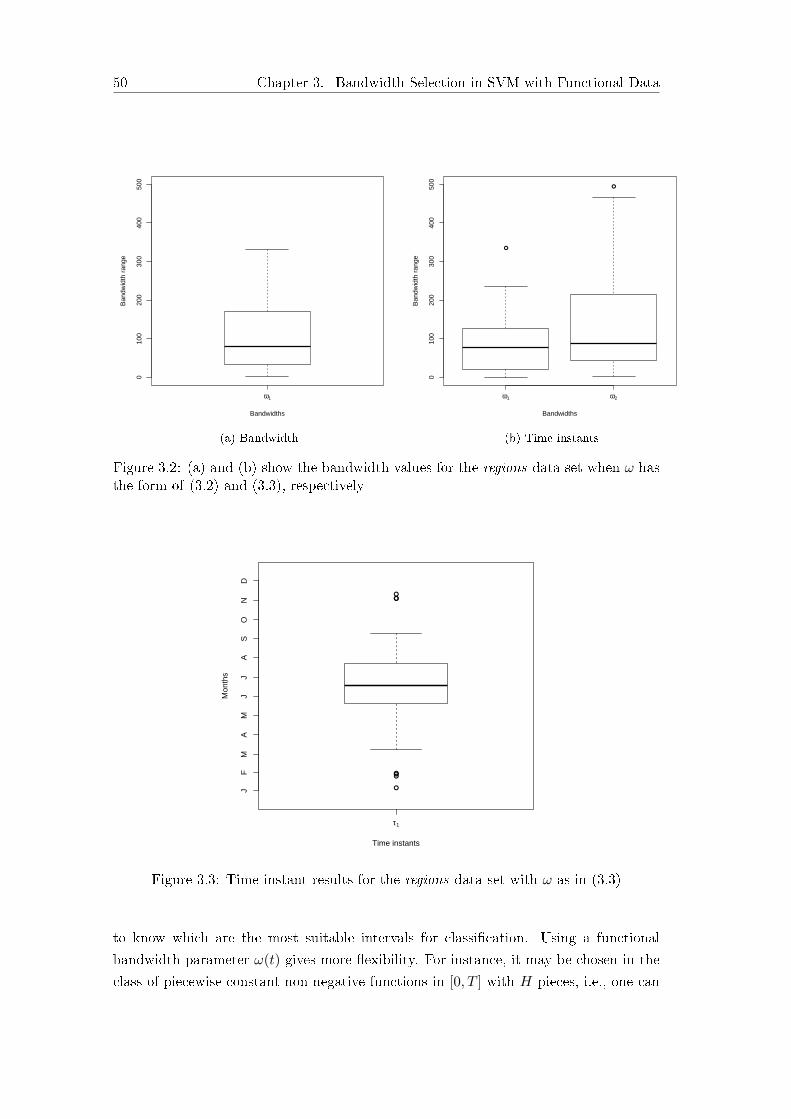
50 Chapter 3. Bandwidth Selection in SVM with Functional Data
ω1
010
020
030
040
050
0
Bandwidths
Ban
dwid
th r
ange
(a) Bandwidth
●
●
ω1 ω2
010
020
030
040
050
0
BandwidthsB
andw
idth
ran
ge
(b) Time instants
Figure 3.2: (a) and (b) show the bandwidth values for the regions data set when ω hasthe form of (3.2) and (3.3), respectively
●
●
●
●
●●
●
τ1
Time instants
Mon
ths
JF
MA
MJ
JA
SO
ND
Figure 3.3: Time instant results for the regions data set with ω as in (3.3)
to know which are the most suitable intervals for classi�cation. Using a functional
bandwidth parameter ω(t) gives more �exibility. For instance, it may be chosen in the
class of piecewise constant non-negative functions in [0, T ] with H pieces, i.e., one can

3.3. Optimal Selection of the Functional Bandwidth 51
naturally assume that ω(t) has the form (3.4)
ω(t) =
ω1, if 0 ≤ t ≤ τ1ω2, if τ1 < t ≤ τ2· · ·ωh, if τh−1 < t ≤ τh· · ·ωH , if τH−1 < t ≤ T
(3.4)
where ω1, . . . , ωH ≥ 0 and 0 ≤ τ1 ≤ . . . ≤ τH−1 ≤ T are parameters to be tuned.
Instead of piecewise constant functions, one could consider ω(t) belonging to the class
of polynomials of degree H which are non-negative in [0, T ], the class of piecewise
polynomial functions non-negative in [0, T ], or the non-negative splines, [De Boor, 1978;
Friedman et al., 2001b].
The use of functional parameters in the kernel may lead to signi�cant improvements
in the accuracy, as demonstrated in our numerical experiments. The price to pay for
obtaining such gains in the accuracy is the fact that tuning the functional parameters
requires the use of using more sophisticated optimization procedures. In Section 3.3 we
detail how the underlying optimization problem for tuning ω(t) is solved.
3.3 Optimal Selection of the Functional Bandwidth
Parameter tuning in the classi�cation of functional data with SVM implies the optimal
choice of two very di�erent elements: the scalar regularization parameter C in (1.15),
and the kernel K in (3.1) through ω(t). The problem of �nding the best function ω(t)
in (3.1) is not tractable as a rule in its full generality. Hence, we restrict our attention
to certain classes of functions parameterized by a vector θ belonging to a certain set Θ,
i.e., ω is expressed as ω(t, θ), and the choice of the function ω is equivalent to choosing
the parameters θ.
Example 3.3.1. For the bandwidth given in (3.4), one would have that
θ = (ω1, . . . , ωH , τ1, . . . , τH−1), and Θ = {(ω1, . . . , ωH , τ1, . . . , τH−1) :
ωh ≥ 0, ∀h, τh ∈ [0, T ], h = 1, . . . ,H − 1, τ1 ≤ . . . ≤ τH−1}. For convenience, we
consider τ0 = 0 and τH = T .
In this chapter, parameter tuning is done following the approach proposed in Chapter
2. First, the data set is divided into k folds. Second, k − 1 folds are again split into
three samples named s1, s2, and s3, while the remaining fold is denoted by s4. Samples
s1 and s2 play the role of training samples, whereas s3 and s4 formed the validation
and testing sets, respectively.
The �rst independent sample s1 is employed for the resolution of Problem (1.15),
that is the classic SVM formulation, to obtain a classi�cation rule by means of α,
for �xed parameters θ and C. The second independent sample s2 is used to measure

52 Chapter 3. Bandwidth Selection in SVM with Functional Data
the quality of parameters θ, i.e., it is used to calculate R((Yi, Y (Xi, θ, α))i∈s2), the
correlation between the class labels and the scores. To �nd the regularization parameter
C, we measure the accuracy in the sample s3 for all the di�erent possible values of C
in the grid, and we keep the C providing the largest accuracy. Finally, the accuracy is
measured in the independent sample s4 is reported.
After all these considerations, for �xed C, we formulate bilevel optimization problem,
that can be expressed as: maxθ,α
R((Yi, Y (Xi, θ, α))i∈s2)
s.t. α solves (1.15) in s1
θ ∈ Θ
(3.5)
We next propose an alternating approach for which only a few iterations will be carried
out. Firstly, in the �rst step of our alternating approach, for �xed parameters θ and
C, a classi�cation rule is obtained solving Problem (1.15), that is, the classic SVM.
Problem (1.15) is a concave quadratic maximization problem, which can be solved by
standard local search optimizers, as speci�ed in Section 1.2.2. Secondly, in the second
step, for �xed α and C, θ is chosen by solving:
maxθ∈Θ
R((Yi, Y (Xi, θ))i∈s2) (3.6)
Problem (3.6) is a continuous optimization problem which is solved by using standard
local search techniques with multi-start. The alternating procedure will alternate these
two steps until some stopping criterion is met. Suitable values for θ and α will be
obtained by this procedure for a speci�c value of the regularization parameter C.
The value of C will be chosen by a grid search, as commonly done in standard SVM.
This means that, for every value of C in a given grid, we measure the accuracy in s3
of the classi�cation rule obtained with the best θ and α found as solutions of Problem
(3.6). The C with the largest accuracy in s3 will be chosen. Finally, we estimate the
correct classi�cation rate using the fourth independent sample, s4.
The pseudocode of the heuristic that have just been presented is outlined in Algo-
rithm 3.
As in Chapter 2, the above-explained methodology is embedded in a nested heuristic.
More precisely, given a family of kernel functions, we construct a series of nested kernel
models with their associated parameters, or equivalently, a series of H nested functional
bandwidths ω(1)(t, θ(1)) ≺ . . . ≺ ω(H)(t, θ(H)). By ω(h)(t, θ(h)) ≺ ω(h+1)(t, θ(h+1)) we
denote that the bandwidth ω(h)(t, θ(h)) has parameters which are part of the parameters
of the bandwidth ω(h+1)(t, θ(h+1)). When solving Problem (3.5) for ω(H)(t, θ(H)) we
will use a sequential approach where the (suboptimal) solution obtained when using
ω(h)(t, θ(h)), will be used as an initial solution of Problem (3.5) with ω(h+1)(t, θ(h+1)).

3.4. Numerical Experiments 53
Algorithm 3 Heuristic for parameter tuning
Input: H• Randomly split the sample s into s1, s2, s3 and s4.for C in the grid do
Alternating Procedurerepeat
1. Fixed θ, compute the parameters α of the SVM classi�er by solvingProblem (1.15) in s1.
2. Fixed α, calculate θ by solving Problem (3.6) in s2.until stopping criteria• Evaluate the accuracy in the sample s3 with C �xed.
end for• The optimal value of C is the one with the best accuracy in s3. The optimal valuesof α and θ are the ones associated with the optimal parameter C.Output: optimal parameters C and θ, optimal classi�cation coe�cients α, and thecorresponding accuracy estimated from s4.
Example 3.3.2. Consider in (3.4) the family of piecewise constant functions with 3
pieces. We have that ω(1)(t, θ(1)) = ω1, with θ(1) = ω1, ω(2)(t, θ(2)) = ω1I[0,τ1] +ω2I(τ1,T ],
with θ(2) = (ω1, ω2, τ1), and �nally ω(3)(t, θ(3)) = ω1I[0,τ1] + ω2I(τ1,τ2] + ω3I(τ2,T ], with
θ(3) = (ω1, ω2, ω3, τ1, τ2). Here I[r,r′] denotes the indicator function, i.e., the function
which is equal to 1 in the interval [r, r′] and 0 otherwise.
Once we have obtained the (suboptimal) solution of ω(h)(t, θ(h)) by
θopt(h) = (ωopt1 , . . . , ωopth , τ opt1 , . . . , τ opth−1), then, we randomly select an interval [τ`−1, τ`) and
split it into two pieces by its midpoint, assigning the same bandwidth value to such two
new pieces. In other words, the initial point of the parameters in the level h + 1 turns
out to be
θ(h+1) =
(ωopt1 , . . . , ωopt`−1, ω
opt` , ωopt` , ωopt`+1, . . . , ω
opth , τ opt1 , . . . , τ opt`−1,
τopt` +τopt`−1
2 , τ opt` , . . . , τ opth
).
The pseudocode of the nested algorithm is shown in Algorithm 4.
3.4 Numerical Experiments
This section details the experiments performed (Section 3.4.1) and the main characte-
ristics of the databases here considered (Section 3.4.2). Finally, Section 3.4.3 presents
the computational results obtained.
3.4.1 Description of the Experiments
In this section, a detailed description of the experiments carried out to test our metho-
dology is made. To obtain stable estimates, k−fold cross-validation has been used to
evaluate the performance of the algorithm on di�erent data sets, as detailed in Section

54 Chapter 3. Bandwidth Selection in SVM with Functional Data
Algorithm 4 Nested heuristic for parameter tuningInput: H, nested functional bandwidths ω(1)(t, θ(1)) ≺ . . . ≺ ω(H)(t, θ(H)).• Randomly split the sample s into s1, s2, s3 and s4.for C in the grid do
Initialization:• h := 1.• Randomly select an initial solution θ(h) ∈ Θ(h).• Set θ := θ(h)
while h ≤ H do1. Using samples s1 and s2, run the Alternating Procedure of Algorithm 3
for ω(t, θ(h)), starting from θ and yielding
θopt(h) =(ωopt1 , . . . , ωopth , τ opt1 , . . . , τ opth−1
)as solution.
2. Randomly select ` ∈ {1, 2, . . . , h}.3. Setθ :=
(ωopt1 , . . . , ωopt`−1, ω
opt` , ωopt` , ωopt`+1, . . . , ω
opth , τopt1 , . . . , τopt`−1,
τopt` +τopt
`−1
2 , τopt` , . . . , τopth−1
)and h := h+ 1.
4. Evaluate the accuracy in the sample s3 with C �xed.end while
end for• For h �xed, the optimal value of C is the one with the best accuracy in s3. Theoptimal values of α and θ(h) are the ones associated to the optimal parameter C.Output: optimal parameters C, θopt(h), ∀h, the associated classi�cation coe�cients α,and the accuracy estimated from s4.
1.2.4. As in the previous chapter, the number k of folds varies depending on the size
of the database. For small databases, k is equal to the number of observations, i.e.,
we performed leave-one-out, whilst for large databases, we take k = 10. A database is
considered small here if and only if it has less than 100 observations. See Table 3.3 for
details.
Algorithm 4 is run k times, one per fold, as done in Chapter 2. Each time, the
division into four independent samples s1, s2, s3, and s4 is done as explained in Section
3.3. The number of runs of the multi-start local search optimization method is set
to �ve. The algorithm is run until the maximum number of iterations reaches ten,
or when the di�erence between the objective values in two consecutive iterations is
less than 10−5. The functional bandwidth ω(t, θ) is the piecewise constant function in
(3.4) with H = 8. The regularization parameter C varies in the set {2−10, . . . , 210}.The parameters θ(h) are in the set Θ(h) = {(ω1, . . . , ωh, τ1, . . . , τh−1) : ω` ≥ 2−4, ` =
1, . . . , h, 0 ≤ τ1 ≤ . . . ≤ τh−1 ≤ T}, ∀h = 1, . . . , 8.
For comparison purposes, apart from the standard SVM, i.e., our approach with
H = 1, we have run three supervised classi�cation methods for functional data, available
at the fda.usc library of R, [Febrero-Bande and Oviedo de la Fuente, 2012], namely
classif.depth, classif.kernel, classif.knn with the default parameters. In order to obtain
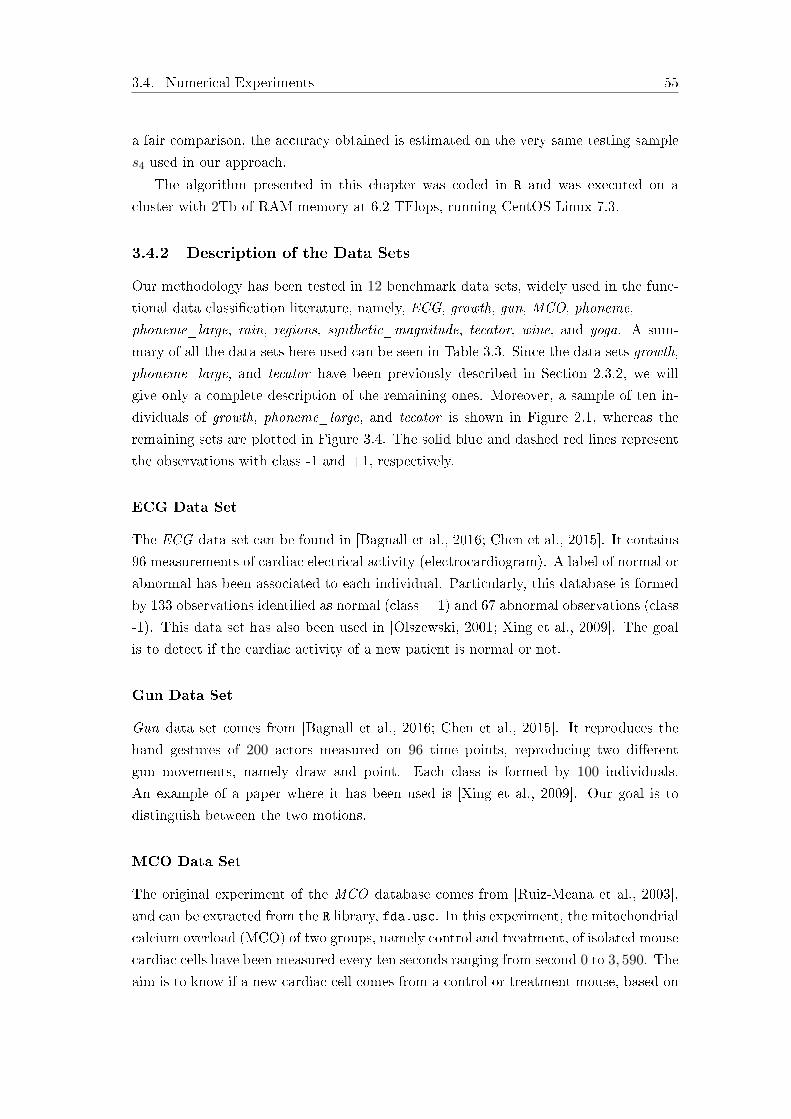
3.4. Numerical Experiments 55
a fair comparison, the accuracy obtained is estimated on the very same testing sample
s4 used in our approach.
The algorithm presented in this chapter was coded in R and was executed on a
cluster with 2Tb of RAM memory at 6.2 TFlops, running CentOS Linux 7.3.
3.4.2 Description of the Data Sets
Our methodology has been tested in 12 benchmark data sets, widely used in the func-
tional data classi�cation literature, namely, ECG, growth, gun, MCO, phoneme,
phoneme_large, rain, regions, synthetic_magnitude, tecator, wine, and yoga. A sum-
mary of all the data sets here used can be seen in Table 3.3. Since the data sets growth,
phoneme_large, and tecator have been previously described in Section 2.3.2, we will
give only a complete description of the remaining ones. Moreover, a sample of ten in-
dividuals of growth, phoneme_large, and tecator is shown in Figure 2.1, whereas the
remaining sets are plotted in Figure 3.4. The solid blue and dashed red lines represent
the observations with class -1 and +1, respectively.
ECG Data Set
The ECG data set can be found in [Bagnall et al., 2016; Chen et al., 2015]. It contains
96 measurements of cardiac electrical activity (electrocardiogram). A label of normal or
abnormal has been associated to each individual. Particularly, this database is formed
by 133 observations identi�ed as normal (class + 1) and 67 abnormal observations (class
-1). This data set has also been used in [Olszewski, 2001; Xing et al., 2009]. The goal
is to detect if the cardiac activity of a new patient is normal or not.
Gun Data Set
Gun data set comes from [Bagnall et al., 2016; Chen et al., 2015]. It reproduces the
hand gestures of 200 actors measured on 96 time points, reproducing two di�erent
gun movements, namely draw and point. Each class is formed by 100 individuals.
An example of a paper where it has been used is [Xing et al., 2009]. Our goal is to
distinguish between the two motions.
MCO Data Set
The original experiment of the MCO database comes from [Ruiz-Meana et al., 2003],
and can be extracted from the R library, fda.usc. In this experiment, the mitochondrial
calcium overload (MCO) of two groups, namely control and treatment, of isolated mouse
cardiac cells have been measured every ten seconds ranging from second 0 to 3, 590. The
aim is to know if a new cardiac cell comes from a control or treatment mouse, based on

56 Chapter 3. Bandwidth Selection in SVM with Functional Data
the MCO levels.This data set has been used in [Baíllo et al., 2011; Cuevas et al., 2006]
and Online companion of [Carrizosa et al., 2014].
Phoneme Data Set
As the phoneme_large data set from Section 2.3.2, the phoneme database was �rst
used in [Hastie et al., 1995]. Here, in the phoneme data set, we use 200 functions, 100
of each class, corresponding to the phonemes �aa� and �ao� as appear in the R library
fda.usc, measured in 150 time points. The objective is to discriminate between the
two phonemes. Some references where this data set has been studied are [Ferraty and
Vieu, 2006; Muñoz and González, 2010; Rossi and Villa, 2006; Torrecilla Noguerales,
2015].
Rain Data Set
The rain data set can be found e.g., in [Martín-Barragán et al., 2014] and contains the
daily temperature measured along a year in 35 Canadian weather stations. Two classes
are distinguished, namely rainy and dry stations, depending if the yearly total amount
of precipitations are below or above 600. The aim is to know if a Canadian station is
dry or not.
Regions Data Set
The regions data set can also be found in e.g., [Martín-Barragán et al., 2014] and
has been already brie�y explained in Example 3.2.1. The objective is to discriminate
between the Atlantic and the rest of climates.
Synthetic_magnitude Data Set
The synthetic_magnitude data set has been simulated from the information detailed
in the Model 3 of [López-Pintado and Romo, 2009]. Particularly, the data have been
recorded on 100 equally-spaced points on the interval [0, 1]. The individuals belonging
to the class +1 have the form:
Xi(t) = 4t+ γi(t), (3.7)
where γi(t) is a stochastic Gaussian process with zero mean and covariance function
c(s, t) = exp (−|t− s|). On the other hand, the observations with label −1 are de�ned
as follows:
Xi(t) =
{4t+ aibiν, if t ≥ Ti4t, if t < Ti
(3.8)
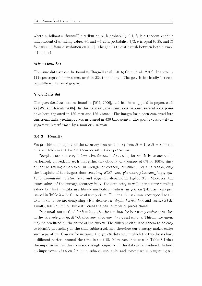
3.4. Numerical Experiments 57
where ai follows a Bernoulli distribution with probability 0.1, bi is a random variable
independent of ai taking values +1 and −1 with probability 1/2, ν is equal to 25, and Tifollows a uniform distribution on [0, 1]. The goal is to distinguish between both classes,
−1 and +1.
Wine Data Set
The wine data set can be found in [Bagnall et al., 2016; Chen et al., 2015]. It contains
111 spectrograph curves measured in 234 time points. The goal is to classify between
two di�erent types of grapes.
Yoga Data Set
The yoga database can be found in [Wei, 2006], and has been applied in papers such
as [Wei and Keogh, 2006]. In this data set, the transitions between several yoga poses
have been captured in 150 men and 156 women. The images have been converted into
functional data, yielding curves measured in 426 time points. The goal is to know if the
yoga pose is performed by a man or a woman.
3.4.3 Results
We provide the boxplots of the accuracy measured on s4 from H = 1 to H = 8 for the
di�erent folds in the k−fold accuracy estimation procedure.
Boxplots are not very informative for small data sets, for which leave-one-out is
performed. Indeed, for each fold either one obtains an accuracy of 0% or 100%, since
either the testing observation is wrongly or correctly classi�ed. For this reason, only
the boxplots of the largest data sets, i.e., ECG, gun, phoneme, phoneme_large, syn-
hetic_magnitude, tecator, wine and yoga, are depicted in Figure 3.6. Moreover, the
exact values of the average accuracy in all the data sets, as well as the corresponding
values for the three fda.usc library methods considered in Section 3.4.1, are also pre-
sented in Table 3.4 for the sake of comparison. The �rst four columns correspond to the
four methods we are comparing with, denoted as depth, kernel, knn and classic SVM.
Finally, last column of Table 3.4 gives the best number of pieces chosen.
In general, our method for h = 2, . . . , 8 is better than the four comparative aproaches
in the data sets growth,MCO, phoneme, phoneme_large, and regions. This improvement
may be produced by the shape of the curves. The di�erent class labels seem to be easy
to identify depending on the time subinterval, and therefore our strategy makes easier
such separation. Observe for instance, the growth data set, in which the two classes have
a di�erent pattern around the time instant 15. Moreover, it is seen in Table 3.4 that
the improvement in the accuracy strongly depends on the data set considered. Indeed,
no improvement is seen for the databases gun, rain, and tecator when comparing our

58 Chapter 3. Bandwidth Selection in SVM with Functional Data
methodology with H = 1 and H ≥ 2. However, for some of the values H ≥ 2 the
accuracy obtained in gun is better than that provided by depth. The results of our
approach in the database rain are always better than the ones provided of the three
fda.usc methods. In contrast, such three methods should be applied if the tecator data
set is studied. In the databases ECG, growth, phoneme_large and yoga there is a minor
improvement (about a 0.5 points) when comparing the classic SVM with our approach
for H ≥ 2. Such improvement also holds in the ECG data set when comparing with
the depth method. The accuracy value obtained in phoneme_large with our approach
when H = 4 pieces are chosen is better than all the three fda.usc methods. Analogous
conclusions are obtained in the yoga data set. A considerably larger accuracy is obtained
in databases MCO, phoneme, regions, synthetic_magnitude, and wine when solving the
problem with H ≥ 2 than when solving with H = 1, i.e., the classic SVM. In some
cases such improvement yields around a ten percentage points of di�erence in accuracy.
Such a large accuracy also occurs when comparing our approach with the three fda.usc
methods in the databasesMCO, regions and wine. The improvement is not so evident in
the phoneme data set. In the data set synthetic_magnitude, our results are comparable
to those provided by depth and knn, but much better than the ones in kernel.
Apart from the improvements in the accuracy, our approach enables us to identify
subintervals of special interest. This fact would be impossible if the standard scalar
bandwidth, which treats equally all time instants, were considered. We highlight, for
instance, the case of the wine data set, whose curves are almost identical except around
the time instants at which peaks occur. Figure 3.5 shows the boxplots of the values of
ω1, ω2, ω3, τ1 and τ2 obtained when a functional bandwidth with H = 3 pieces is sought.
We observe that the time instants which distinguish one piece from another are around
50 and 125, which coincides with the points of some of the peaks. Furthermore, the
associated weight is greater in the third part, where the biggest peak is located.
Regarding the trajectory of the accuracy versus the number of pieces, we observe
that there is not a clear pattern. For instance, in the MCO data set, we have worse
results with H = 2 pieces than with the classic SVM (H = 1). However, a di�erence of
six points is obtained when comparing H = 6 with H = 1.
In contrast, in the regions data set, the accuracies with H ≥ 2 are signi�cantly
better than with H = 1, reaching the maximum value with H = 6. Similar conclusions
can be drawn in the remaining data sets.
This fact shows that a good choice of the value of H is necessary. Since the value of
the parameter H depends on the division of the data set, we show in the last column
of Table 3.4 the average value of the best H parameter estimated on sample s3.

3.5. Conclusions and Extensions 59
#records #points measurements #records label -1 #records label +1
ECG 200 96 67 133growth 93 31 54 39gun 200 96 100 100MCO 89 360 44 45
phoneme 200 150 100 100phoneme_large 1717 256 1022 695
rain 35 365 15 20regions 35 365 20 15
synthetic_magnitude 150 100 75 75tecator 215 100 77 138wine 111 234 54 57yoga 306 426 150 156
Table 3.3: Data description summary
3.5 Conclusions and Extensions
In this chapter, we have shown how SVM for functional data can be improved if a
functional bandwidth, to be tuned via a nested heuristic, is used. By using very simple
functional parameters, together with our tuning procedure, we obtained better accuracy
in the test sets than with the traditional scalar parameter model. The methodology here
proposed is able to identify the critical points in which a change in the behavior of the
functions is produced, yielding the most relevant intervals in terms of the classi�cation
rate.
The di�culties associated to the tuning of more complex structures are mitigated by
the use of a heuristic that exploits the nested structure of the functional parameter, by
using the (suboptimal) solution of one level as an initial solution for the next level. Our
tuning procedure takes advantage of the functional nature of the data by expressing the
tuning problem as a bilevel optimization problem in continuous variables. In contrast to
the usual approach, where the misclassi�cation rate is minimized, here the correlation
between labels and scores are optimized, allowing us to use gradient-based local search
algorithms.
In our approach, the number of pieces of the functional bandwidth, H, is �xed from
the beginning, and the trajectory of the classi�cation rates for the di�erent number of
pieces is shown. However, since the results depend on H, we also choose the value of
H yielding the best accuracy, estimated on the validation sample.
The analysis performed here, using piecewise constant functions as bandwidths, can
be easily extended to other expressions such as polynomials, or piecewise polynomials,
including splines [De Boor, 1978; Friedman et al., 2001b]. Apart from the Pearson
correlation coe�cient, di�erent types of association measures can be applied, [Székely
et al., 2007; Torrecilla Noguerales, 2015].

60 Chapter 3. Bandwidth Selection in SVM with Functional Data
The functional data here considered are univariate functions. The case of multi-
variate (hybrid) functional data, [Jiménez-Cordero and Maldonado, 2018] can also be
addressed with our proposal, after the convenient modi�cation of the kernel function.
The standard hinge loss function has been used in the SVM formulation of this
chapter. Our approach might also be adapted to other loss functions, such as the
so-called ramp loss, [Brooks, 2011], by replacing (1.15) with the corresponding SVM
problem. The same happens if the SVM in (1.15) is replaced by other related methods
such as the least-squares SVM, e.g., [Cruz-Cano et al., 2010].
Our approach is limited here to classi�cation problems. If instead, functional regres-
sion is pursued, [Sood et al., 2009], our methodology can be adapted to this context,
replacing SVM by Support Vector Regression (SVR).

3.5. Conclusions and Extensions 61
0 20 40 60 80
−20
−10
010
2030
Time
Ele
ctro
card
iogr
am s
igna
ls
NormalAbnormal
(a) ECG
0 50 100 150
−20
−10
010
20
Time
Gun
Tra
yect
ory
DrawPoint
(b) gun
0 500 1000 1500 2000 2500 3000 3500
050
010
0015
0020
0025
00
Seconds
Leve
l of M
itoch
ondr
ial C
alci
um Io
n
ControlTreatment
(c) MCO
0 50 100 150
510
1520
25
Time
Log−
perio
dogr
ams
aoaa
(d) phoneme
−30
−20
−10
010
20
Months
Tem
pera
ture
J F M A M J J A S O N D
RainyDry
(e) rain
−30
−20
−10
010
20
Months
Tem
pera
ture
J F M A M J J A S O N D
AtlanticRest
(f) regions
Figure 3.4: Sample of functional data in the data sets analyzed

62 Chapter 3. Bandwidth Selection in SVM with Functional Data
0.0 0.2 0.4 0.6 0.8 1.0
−25
−20
−15
−10
−5
05
Time
Dat
a
Label −1Label 1
(g) synthetic_magnitude
0 50 100 150 200
−2
−1
01
23
Time
Spe
ctra
Grape aGrape b
(h) wine
0 100 200 300 400
−2
−1
01
2
Time
Yoga
Pos
es P
rofil
e
MaleFemale
(i) yoga
Figure 3.4: Sample of functional data in the real data sets analyzed (cont.)
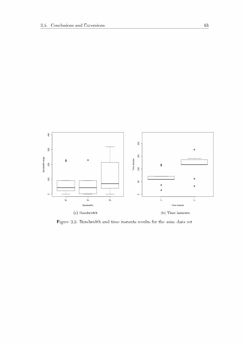
3.5. Conclusions and Extensions 63
●● ●
ω1 ω2 ω3
010
020
030
040
0
Bandwidths
Ban
dwid
th r
ange
(a) Bandwidth
●●
●
●
●
●
●
τ1 τ2
050
100
150
200
Time instants
Tim
e do
mai
n
(b) Time instants
Figure 3.5: Bandwidth and time instants results for the wine data set

64 Chapter 3. Bandwidth Selection in SVM with Functional Data
●●●
●●●●●
●●●
●
●
●
●●●●●
●●
40
60
80
100
ECG gun
phoneme
phoneme_large
synthetic_magnitude
tecatorwine
yoga
Databases
Acc
urac
y (%
)
#pieces, H
1
2
3
4
5
6
7
8
Figure 3.6: Accuracy boxplots in the analyzed larger data sets depending on the numberof pieces, H. Since the boxplots are rather informative for the small data sets, i.e.,growth, MCO, rain and regions, only the accuracy values of the remaining databasesare depicted

3.5. Conclusions and Extensions 65
depth
kernel
knn
HBestH
1(classicSV
M)
23
45
67
8ECG
67.51
74.41
83.92
67.51
67.5167.5168.0168.0168.0168.0168.01
1.70
growth
78.49
94.62
92.47
94.62
94.6294.6294.6293.5495.6994.6294.62
1.30
gun
52.50
73.50
78.00
69.50
68.0069.5069.5067.5067.0069.0069.50
3.00
MCO
67.41
78.65
79.77
80.89
78.6583.1482.0283.1486.5183.1483.14
4.15
phonem
e76.00
80.00
73.50
80.50
81.5081.0081.5082.0081.0080.5080.50
4.00
phonem
e_large
71.69
65.46
78.91
81.24
81.4781.2482.0081.6581.5981.8381.65
2.10
rain
82.85
80.00
77.14
82.85
80.0080.0082.8580.0080.0077.1477.14
1.91
regions
77.14
85.71
77.14
82.84
88.5688.5788.5785.7191.4291.4288.57
1.77
synthetic_magnitude
99.37
55.97
96.54
90.40
91.1190.4092.5492.5492.5492.5492.54
1.90
tecator
94.87
98.13
98.11
74.04
74.0474.0474.0474.0474.0473.5974.04
1.80
wine
61.87
91.93
92.03
71.27
75.7777.5977.5975.6876.6876.6876.68
2.60
yoga
84.13
96.08
96.73
95.11
95.4595.7696.4495.7896.0996.0996.09
3.60
Table
3.4:
Average
oftheaccuracy
estimated
onsamples 4
forallthedata
sets
afterrunn
ingthethreemethods
availableat
fda.usc
(depth,kernel
andknn)andrunn
ingourapproach
from
H=
1toH
=8.
Lastcolumnpresents
theaveragevalueof
thebestparameter
H


Chapter 4
SVM-Classi�cation of Hybrid
Functional Data
67


4.1. Introduction 69
4.1 Introduction
In this chapter, we are interested in classifying hybrid functional data, i.e., data with
functional and static (constant over time) covariates, into two prede�ned classes, using
SVM. Feature selection plays a very important role in data mining. Hence, it is crucial
to design a methodology that selects the most important features yielding good classi-
�cation performance. Some references of feature selection and particularly, on feature
selection in univariate functional data are given in Section 1.3. Nevertheless, regard-
ing feature selection in multivariate functional data and, more speci�cally, in hybrid
functional data, the literature is very scarce.
In this chapter, we demonstrate that hybrid data sets cannot be learned properly
with the current methodologies for SVM classi�cation. We propose a modi�cation of the
standard SVM classi�cation to handle functional hybrid data sets, and as a byproduct,
to select the most informative features. The di�erent components of the data, functional
or static, are weighted by di�erent scaling factors of a modi�ed Gaussian kernel. The
idea of considering di�erent weights for di�erent types of features is not new. Indeed,
it has been applied in [Bugeau and Pérez, 2007; Chen et al., 2000; Duong et al., 2008;
Sain, 2002] for kernel density estimation purposes and in [Maldonado et al., 2015] for
clustering problems, among others.
The remainder of this chapter is structured as follows: in Section 4.2 we formally
introduce the concepts used in our methodology and detail our approach. Section
4.3 is devoted to the computational experience, including a sensitivity analysis of the
parameters involved in the model. Finally, some conclusions and possible future lines
of research are described in Section 4.4.
4.2 The Mathematical Model
This section details the problem formulation of feature selection in SVM classi�cation
with hybrid functional data, as well as the solving strategy.
Following the notation of previous chapters, let s be a sample of individuals with an
associated pair (Xi, Yi) for each individual i ∈ s. A hybrid functional datum Xi ∈ X ,with X = Fp1 × Rp2 , is de�ned as a vector of p1 functional features and p2 static
features, as in Equation (1.2), for a Hilbert space F . Moreover, Yi ∈ {−1,+1} denotesthe class label of the observation i ∈ s.
In this chapter we design a model which obtains, via SVM, good classi�cation rates
in order to determine the class Y of a new observation X ∈ X , and at the same time it
yields the most informative set of features V ⊂ {1, . . . , p1 + p2}.To do this, we use the kernel function given in (1.26) in which a scalar bandwidth is
associated to each feature, instead of the usual isotropic Gaussian kernel with a unique
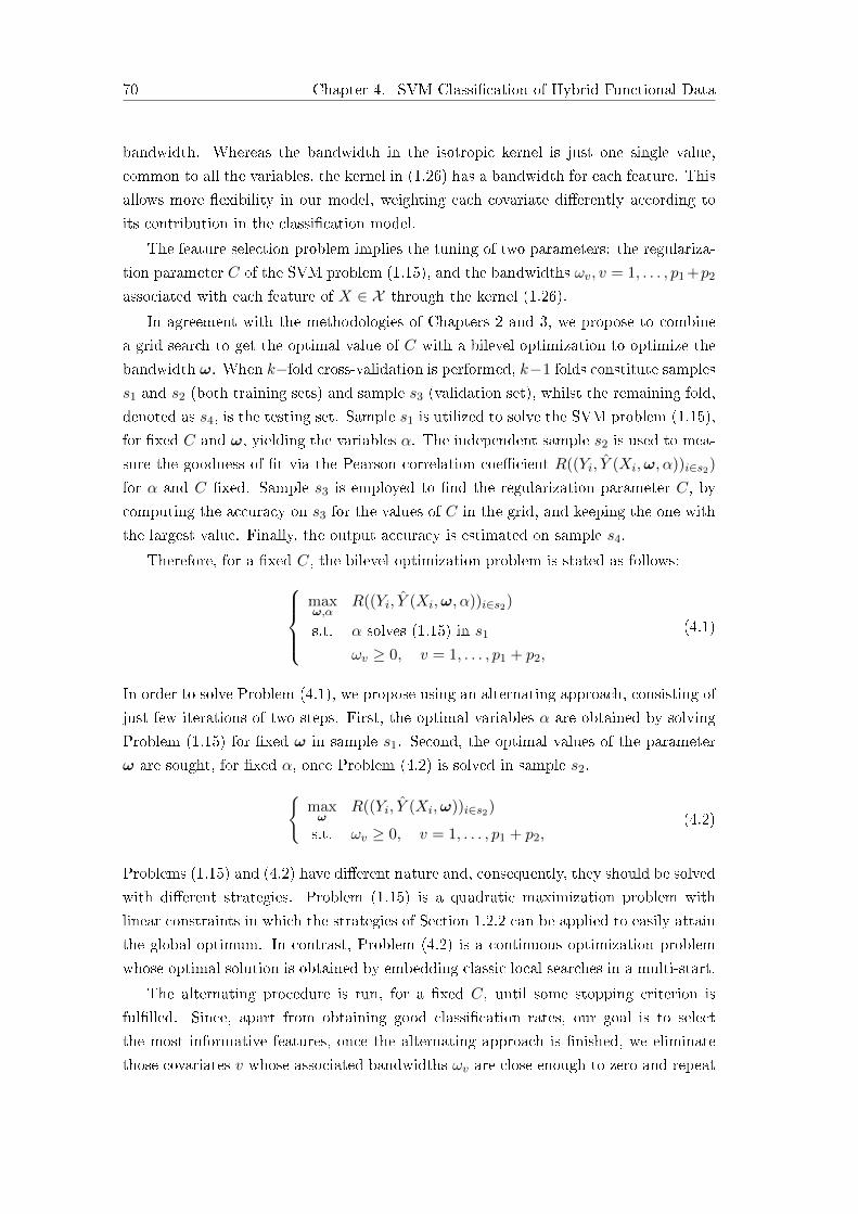
70 Chapter 4. SVM-Classi�cation of Hybrid Functional Data
bandwidth. Whereas the bandwidth in the isotropic kernel is just one single value,
common to all the variables, the kernel in (1.26) has a bandwidth for each feature. This
allows more �exibility in our model, weighting each covariate di�erently according to
its contribution in the classi�cation model.
The feature selection problem implies the tuning of two parameters: the regulariza-
tion parameter C of the SVM problem (1.15), and the bandwidths ωv, v = 1, . . . , p1 +p2
associated with each feature of X ∈ X through the kernel (1.26).
In agreement with the methodologies of Chapters 2 and 3, we propose to combine
a grid search to get the optimal value of C with a bilevel optimization to optimize the
bandwidth ω. When k−fold cross-validation is performed, k−1 folds constitute samples
s1 and s2 (both training sets) and sample s3 (validation set), whilst the remaining fold,
denoted as s4, is the testing set. Sample s1 is utilized to solve the SVM problem (1.15),
for �xed C and ω, yielding the variables α. The independent sample s2 is used to mea-
sure the goodness of �t via the Pearson correlation coe�cient R((Yi, Y (Xi,ω, α))i∈s2)
for α and C �xed. Sample s3 is employed to �nd the regularization parameter C, by
computing the accuracy on s3 for the values of C in the grid, and keeping the one with
the largest value. Finally, the output accuracy is estimated on sample s4.
Therefore, for a �xed C, the bilevel optimization problem is stated as follows:maxω,α
R((Yi, Y (Xi,ω, α))i∈s2)
s.t. α solves (1.15) in s1
ωv ≥ 0, v = 1, . . . , p1 + p2,
(4.1)
In order to solve Problem (4.1), we propose using an alternating approach, consisting of
just few iterations of two steps. First, the optimal variables α are obtained by solving
Problem (1.15) for �xed ω in sample s1. Second, the optimal values of the parameter
ω are sought, for �xed α, once Problem (4.2) is solved in sample s2.{maxω
R((Yi, Y (Xi,ω))i∈s2)
s.t. ωv ≥ 0, v = 1, . . . , p1 + p2,(4.2)
Problems (1.15) and (4.2) have di�erent nature and, consequently, they should be solved
with di�erent strategies. Problem (1.15) is a quadratic maximization problem with
linear constraints in which the strategies of Section 1.2.2 can be applied to easily attain
the global optimum. In contrast, Problem (4.2) is a continuous optimization problem
whose optimal solution is obtained by embedding classic local searches in a multi-start.
The alternating procedure is run, for a �xed C, until some stopping criterion is
ful�lled. Since, apart from obtaining good classi�cation rates, our goal is to select
the most informative features, once the alternating approach is �nished, we eliminate
those covariates v whose associated bandwidths ωv are close enough to zero and repeat

4.3. Numerical Experiments 71
the alternating algorithm with the remaining features. In other words, we keep those
features satisfying ωv > δ, where δ > 0 is a threshold value. This process is repeated
until the selected features do not change in two consecutive iterations of the procedure
that has just been described.
Once the alternating approach has provided good values for α, ω, and therefore, the
set V of selected features, the value of C is chosen by computing the accuracy on s3 for
all C values in the grid, and the one that leads to the largest accuracy is kept.
Finally, the e�ectiveness of our methodology is tested on an independent sample s4,
in which the classi�cation accuracy is computed.
The pseudocode of our approach is given in Algorithm 5.
Algorithm 5 Heuristic for parameter tuning and feature selection
• Randomly split the sample s into s1, s2, s3 and s4.for C in the grid do
Initialization: V = {1, . . . , p1 + p2}repeat
Alternating Procedurerepeat
1. For ω �xed, obtain the variables α of the SVM classi�er by solvingProblem (1.15) in s1.
2. For a �xed α, calculate ω by solving Problem (4.2) in s2.until stopping criteria• Delete the features, v, such that ωv ≤ δ, i.e., V = {v : ωv > δ}
until no new features are deleted• Evaluate the accuracy in the sample s3 with C �xed.
end for• Keep the value of C with the maximum accuracy in s3, and the associated valuesof α, ω, and the set V.Output: optimal parameters C and ω, optimal classi�cation coe�cients α, the se-lected features in V, and the corresponding accuracy estimated from s4.
4.3 Numerical Experiments
This section is devoted to the computational experience on the algorithm proposed in
this chapter for classi�cation and feature selection of hybrid functional data. Section
4.3.1 is devoted to the description of the experiments performed. In Section 4.3.2,
the di�erent databases are described. Section 4.3.3 presents several algorithms used to
compare our proposed methodology. Finally, Section 4.3.4 outlines the details of the
sensitivity analysis, and Section 4.3.5 gives the results of our proposal.

72 Chapter 4. SVM-Classi�cation of Hybrid Functional Data
4.3.1 Description of the Experiments
This section explains the details of the computational experiments carried out to show
the e�ciency of our approach. Algorithm 5 has been run on the databases described
in Section 4.3.2. Each data set is split into four parts, s1 − s4, as explained in Section
4.2. Since the features of the hybrid functional data may have di�erent scales, we have
normalized them before applying our approach, as explained in e.g., [Wang and Yao,
2015].
When selecting the most informative covariates, we remove those features with
ωv ≤ 10−5, i.e., δ = 10−5. The stopping criterion is ful�lled when the number of itera-
tions is equal to �ve. The parameter C ranges in the set {2−7, . . . , 27} on a logarithmic
scale.
In order to have stable results, Algorithm 5 was run �ve times, and the boxplot of
the accuracy computed on s4 is reported. To compare our methodology with others, we
consider the approaches detailed in Section 4.3.3.
Furthermore, we executed a sensitivity analysis of the parameters involved in the
algorithm. The details of this analysis are shown in Section 4.3.4.
All the experiments were coded in R, [Core Team, 2017], and carried out in a cluster
with 2 terabytes of RAM memory at 6.2 TFlops, running CentOS Linux 7.3.
4.3.2 Description of the Data Sets
Two simulated examples, namely batch and trigonometric, and two real databases, de-
noted here as pen and retail, were considered. A summarized description of the data
sets, including the number of individuals in the sample, the number of elements of each
class, and the number of static and functional covariates, is given in Table 4.1.
#individuals #functional #static #records #recordscovariates covariates label -1 label +1
batch 1000 3 2 500 500trigonometric 1000 2 2 500 500pen 296 2 1 171 125retail 3602 5 1 1776 1826
Table 4.1: Data description summary
The functional covariates of batch and trigonometric data sets have already been
explained in Section 2.3.2, more speci�cally on Equations (2.8) and (2.9), respectively.
Therefore, in this section we will only provide the details of their static covariates. By
contrast, a complete description of the databases pen and retail is given. Figures 4.1-4.4
show respectively a subset of ten functions of the four data sets. The functional features

4.3. Numerical Experiments 73
are depicted in a standard x−y plot, where the solid blue lines and the dashed red lines
indicate respectively the individuals with class −1 and +1. On the other hand, for the
sake of visualization, static covariates are shown in boxplots (or barplots in the case of
categorical features), with the individuals with classes −1 and +1 colored in blue and
red respectively.
0.0 0.4 0.8
01
23
45
6
Time
Fea
ture
1
0.0 0.4 0.8
01
23
45
6
Time
Fea
ture
2
0.0 0.4 0.8
05
1015
Time
Fea
ture
3
Label −1Label +1
●
●
−1 +1
38.5
39.5
40.5
41.5
Fea
ture
4
●
−1 +1
01
23
4
Fea
ture
5
Figure 4.1: Sample of batch data set
Batch data set
The three functional covariates of the �rst data set, batch, are given in Equation (2.8).
Note that the class label Yi just depends on the value ν0 in the de�nition of X3. There-
fore, the third covariate is the only relevant feature for classi�cation, if just the functional
components of the hybrid functional data is taken into account.
To complete the data set, we added two real variables, X4 and X5, in agreement
with (4.3) and (4.4) for all i = 1, . . . , 1000:
Xi4 ∼
N (µ = 39, σ2 = 1), if Yi = +1
N (µ = 40, σ2 = 1), if Yi = −1
(4.3)

74 Chapter 4. SVM-Classi�cation of Hybrid Functional Data
5 10 15 20
−10
−5
05
10
Time
Fea
ture
1
5 10 15 20
−10
1030
50
Time
Fea
ture
2
Label −1 Label +1
●
−1 +1
1020
3040
50
Fea
ture
3
●
●
●
−1 +1
−2
−1
01
2
Fea
ture
4
Figure 4.2: Sample of trigonometric data set
Xi5 ∼
N (µ = 2, σ2 = 1), if Yi = +1
N (µ = 3, σ2 = 1), if Yi = −1
(4.4)
where N (µ, σ2) indicates a normal distribution of mean µ and variance σ2.
Trigonometric data set
The trigonometric database consists two functional features and two scalar covariates.
Functional components are shown in Equation (2.9).
The remaining static variables X3 and X4 have been created according to (4.5) and
(4.6)
Xi3 ∼
N (µ = 0, σ2 = 225), if Yi = +1
N (µ = 20, σ2 = 400), if Yi = −1
(4.5)
Xi4 ∼ N (µ = 0, σ2 = 1), ∀i (4.6)
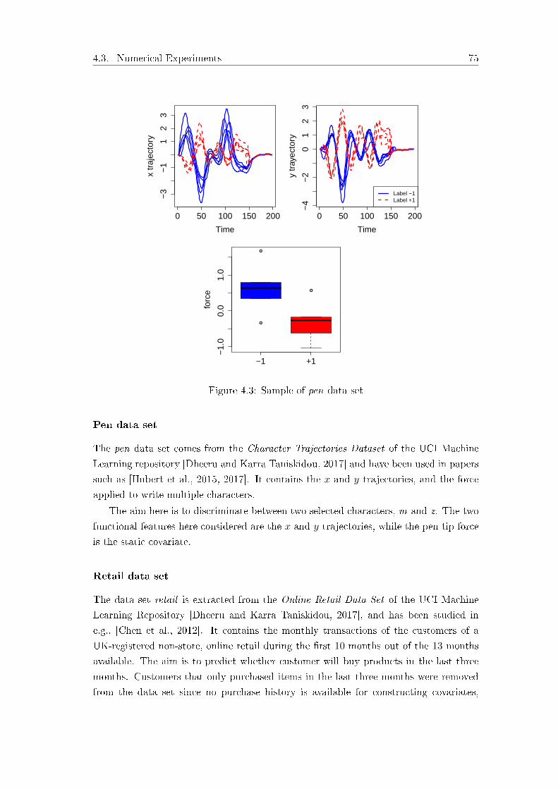
4.3. Numerical Experiments 75
0 50 100 150 200
−3
−1
12
3
Time
x tr
ajec
tory
0 50 100 150 200
−4
−2
01
23
Time
y tr
ayec
tory
Label −1Label +1
●
●
●
−1 +1
−1.
00.
01.
0
forc
e
Figure 4.3: Sample of pen data set
Pen data set
The pen data set comes from the Character Trajectories Dataset of the UCI Machine
Learning repository [Dheeru and Karra Taniskidou, 2017] and have been used in papers
such as [Hubert et al., 2015, 2017]. It contains the x and y trajectories, and the force
applied to write multiple characters.
The aim here is to discriminate between two selected characters, m and z. The two
functional features here considered are the x and y trajectories, while the pen tip force
is the static covariate.
Retail data set
The data set retail is extracted from the Online Retail Data Set of the UCI Machine
Learning Repository [Dheeru and Karra Taniskidou, 2017], and has been studied in
e.g., [Chen et al., 2012]. It contains the monthly transactions of the customers of a
UK-registered non-store, online retail during the �rst 10 months out of the 13 months
available. The aim is to predict whether customer will buy products in the last three
months. Customers that only purchased items in the last three months were removed
from the data set since no purchase history is available for constructing covariates,

76 Chapter 4. SVM-Classi�cation of Hybrid Functional Data
2 4 6 8 10
040
080
0
Months
Am
ount
2 4 6 8 10
010
025
0
Months
Qua
ntity
2 4 6 8 10
02
46
8
Months
Rec
ency
2 4 6 8 10
01
23
45
6Months
Fre
quen
cy
2 4 6 8 10
040
080
0
Months
Mon
etar
y
Label −1Label +1
Yes No
UK
cus
tom
er?
02
46
810
Figure 4.4: Sample of retail data set
yielding an amount of 3,602 individuals instead of the original number of 3,630. The
�rst functional feature is the amount of money spent by the customers. The second
functional variable denotes the quantity of products bought. The last three functional
covariates are the variables Recency, Frequency, and Monetary, described in [Chen et
al., 2012]. Finally, the scalar variable is a binary feature which indicates whether the
customers come from the UK, or not.
4.3.3 Comparative Algorithms
Since, to the best of our knowledge, no methodology has been reported in the literature
of classi�cation to deal with feature selection in hybrid functional data, we suggest some
techniques with which to compare our proposal, described in what follows.
Functional SVM (FSVM)
The �rst alternative method corresponds to the SVM algorithm for functional data. In
this case, the di�erent types of features, i.e., functional or static, are not taken into
account, and no variable selection is made.
A grid search is performed to obtain the scalar parameters C and ω based on the

4.3. Numerical Experiments 77
following set of values: {2−7, . . . , 27} on a logarithmic scale. The SVM problem (1.15)
is solved with an isotropic Gaussian kernel in (4.7):
K(Xi, Xj , ω) = exp
−ω p1∑v=1
∫ T
0(Xiv(t)−Xjv(t))
2 dt+
p2∑v=p1+1
(Xiv −Xjv)2
(4.7)
for Xi, Xj ∈ X . The scalar parameters C and ω yielding the best accuracy in the
validation sample are kept. Finally, the accuracy for the selected parameters C and ω
is computed as a measure of performance.
Static SVM (SSVM)
The second alternative corresponds to the SVM problem when the functions of the
hybrid functional data are summarized in scalar values.
We solved the SVM problem (1.15) on the training set, for each of the values of C
and ω belonging to the set {2−7, . . . , 27} in logarithmic scale. The best values of C and
ω are chosen by measuring the accuracy on the validation sample, and then, the �nal
results are estimated with the optimal values for C and ω on the testing sample.
In this case, the kernel function used in Problem (1.15) is the isotropic kernel in
(1.22) for multivariate data, K(Zi, Zj), in which a transformation of Xi, namely Zi,
is used. Two di�erent transformations Zi are here suggested. In the �rst one, each
functional component Xiv(t), v = 1, . . . , p1 is summarized in a 4−dimensional vector
which includes the mean value, the standard deviation, the minimum and the maximum
values. Moreover, we add the values of the static covariates Xiv, v = p1 +1, . . . , p1 +p2.
Such transformation Zi is given in (4.8):
Zi =(mean(Xi1(t)), sd(Xi1(t)), min(Xi1(t)), max(Xi1(t)), . . . ,
mean(Xip(t)), sd(Xip(t)), min(Xip(t)), max(Xip(t)),
Xi p1+1, . . . , Xi p1+p2
)(4.8)
The second transformation proposed consists of substituting each functional covariate
by its value at the H discretization points, t1, . . . , tH , where it has been recorded. We
also add the values of the static covariates. In other words, the transformation Zi turns
out to be as in (4.9):
Zi =(Xi1(t1), . . . , Xi1(tH), . . . , Xip1(t1), . . . , Xip1(tH), Xi p1+1, . . . , Xi p1+p2
)(4.9)
LiblineaR
The last comparative algorithm comes from the R library LiblineaR. Such library com-
bines di�erent types of loss functions and regularization schemes, yielding eight versions
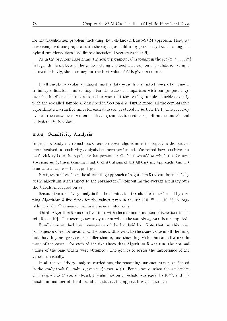
78 Chapter 4. SVM-Classi�cation of Hybrid Functional Data
for the classi�cation problem, including the well-known Lasso-SVM approach. Here, we
have compared our proposal with the eight possibilities by previously transforming the
hybrid functional data into �nite-dimensional vectors as in (4.9).
As in the previous algorithms, the scalar parameter C is sought in the set {2−7, . . . , 27}in logarithmic scale, and the value yielding the best accuracy on the validation sample
is saved. Finally, the accuracy for the best value of C is given as result.
In all the above-explained algorithms the data set is divided into three parts, namely,
training, validation, and testing. For the sake of comparison with our proposed ap-
proach, the division is made in such a way that the testing sample coincides exactly
with the so-called sample s4 described in Section 4.2. Furthermore, all the comparative
algorithms were run �ve times for each data set, as stated in Section 4.3.1. The accuracy
over all the runs, measured on the testing sample, is used as a performance metric and
is depicted in boxplots.
4.3.4 Sensitivity Analysis
In order to study the robustness of our proposed algorithm with respect to the param-
eters involved, a sensitivity analysis has been performed. We tested how sensitive our
methodology is to the regularization parameter C, the threshold at which the features
are removed δ, the maximum number of iterations of the alternating approach, and the
bandwidths ωv, v = 1, . . . , p1 + p2.
First, we ran �ve times the alternating approach of Algorithm 5 to test the sensitivity
of the algorithm with respect to the parameter C, computing the average accuracy over
the k folds, measured on s3.
Second, the sensitivity analysis for the elimination threshold δ is performed by run-
ning Algorithm 5 �ve times for the values given in the set {10−10, . . . , 10−5} in loga-
rithmic scale. The average accuracy is estimated on s3.
Third, Algorithm 5 was run �ve times with the maximum number of iterations in the
set {5, . . . , 10}. The average accuracy measured on the sample s3 was then computed.
Finally, we studied the convergence of the bandwidths. Note that, in this case,
convergence does not mean that the bandwidths tend to the same value in all the runs,
but that they are greater or smaller than δ, and thus they yield the same features in
most of the cases. For each of the �ve times that Algorithm 5 was run, the optimal
values of the bandwidths were obtained. The goal is to assess the importance of the
variables visually.
In all the sensitivity analyses carried out, the remaining parameters not considered
in the study took the values given in Section 4.3.1. For instance, when the sensitivity
with respect to C was analyzed, the elimination threshold was equal to 10−5, and the
maximum number of iterations of the alternating approach was set to �ve.

4.3. Numerical Experiments 79
● ● ● ● ● ●
●●
● ● ●
●
● ● ●
5060
7080
9010
0
C
Acc
urac
y (%
)
2−7 2−6 2−5 2−4 2−3 2−2 2−1 20 21 22 23 24 25 26 27
(a) Sensitivity analysis (C)
● ● ● ● ● ●
5060
7080
9010
0
δ
Acc
urac
y (%
)
10−10 10−9 10−8 10−7 10−6 10−5
(b) Sensitivity analysis (δ)
● ● ● ● ● ●
5060
7080
9010
0
iterations
Acc
urac
y (%
)
5 6 7 8 9 10
(c) Sensitivity analysis (number iterations)
Figure 4.5: Results of the sensitivity analysis for the batch data set
4.3.5 Results
Algorithm 5 and all the comparative methods of Section 4.3.3 have been run �ve times.
Boxplots of the accuracy on the testing sample are given to test the e�ciency of our
proposal. Particularly, in the boxplots, our approach is denoted by alt, and the FSVM
strategy of Section 4.3.3 is marked as f, the SSVMmethod for the �nite-dimensional data
in (4.8) and (4.9) are denoted by st and disc, respectively, �nally, the accuracy results
of the eight classi�cation methodologies of LiblineaR in Section 4.3.3 are indicated by
r0, r1, . . . , r7, since the parameter in the R function that states which out of the eight
methods is used, goes from 0 to 7.
Plots of the results of sensitivity analysis explained in Section 4.3.4, are also depicted

80 Chapter 4. SVM-Classi�cation of Hybrid Functional Data
050
100
150
200
Iterations of feature deletion
Ban
dwid
th
●● ●
●
Feature 1Feature 2Feature 3Feature 4Feature 5
Initialization 1 2
(a) Run 10
5010
015
020
0
Iterations of feature deletion
Ban
dwid
th
● ● ●
●
Feature 1Feature 2Feature 3Feature 4Feature 5
Initialization 1 2
(b) Run 2
050
100
150
200
Iterations of feature deletion
Ban
dwid
th
●
● ●
●
Feature 1Feature 2Feature 3Feature 4Feature 5
Initialization 1 2
(c) Run 3
050
100
150
200
Iterations of feature deletion
Ban
dwid
th
●
● ● ●
●
Feature 1Feature 2Feature 3Feature 4Feature 5
Initialization 1 2 3
(d) Run 4
050
100
150
200
Iterations of feature deletion
Ban
dwid
th
●
● ●
●
Feature 1Feature 2Feature 3Feature 4Feature 5
Initialization 1 2
(e) Run 5
Figure 4.6: Convergence of the bandwidths for the batch data set

4.3. Numerical Experiments 81
● ●●
●
●
●
● ●● ● ● ●
●
● ●
5060
7080
9010
0
C
Acc
urac
y (%
)
2−7 2−6 2−5 2−4 2−3 2−2 2−1 20 21 22 23 24 25 26 27
(a) Sensitivity analysis (C)
● ● ● ● ● ●
5060
7080
9010
0
δ
Acc
urac
y (%
)
10−10 10−9 10−8 10−7 10−6 10−5
(b) Sensitivity analysis (δ)
● ● ● ● ● ●
5060
7080
9010
0
iterations
Acc
urac
y (%
)
5 6 7 8 9 10
(c) Sensitivity analysis (number iterations)
Figure 4.7: Results of the sensitivity analysis for the trigonometric data set
in Figures 4.5 - 4.12.
More details about the classi�cation performance on the tested data sets are given
in the following lines.
Batch data set
Figure 4.13 shows the boxplots of the accuracy when comparing our proposal and the
remaining methods. It is quite apparent that the proposed methodology yields better
accuracy and we are able to identify the most informative features as a byproduct. In
fact, the third variable was selected to be important by our algorithm in all the �ve
runs. Remember that this feature is the only functional covariate which is correlated
with the target variable. In the third run, for instance, we obtain the following optimal

82 Chapter 4. SVM-Classi�cation of Hybrid Functional Data
020
4060
8010
0
Iterations of feature deletion
Ban
dwid
th
●
●
●
●
Feature 1Feature 2Feature 3Feature 4
Initialization 1 2
(a) Run 10
2040
6080
100
Iterations of feature deletion
Ban
dwid
th
●
●
●
Feature 1Feature 2Feature 3Feature 4
Initialization 1
(b) Run 2
020
4060
8010
0
Iterations of feature deletion
Ban
dwid
th
●
● ●
●
Feature 1Feature 2Feature 3Feature 4
Initialization 1 2
(c) Run 3
020
4060
8010
0
Iterations of feature deletion
Ban
dwid
th
●
● ●
●
Feature 1Feature 2Feature 3Feature 4
Initialization 1 2
(d) Run 4
020
4060
8010
0
Iterations of feature deletion
Ban
dwid
th
●
● ● ●
●
Feature 1Feature 2Feature 3Feature 4
Initialization 1 2 3
(e) Run 5
Figure 4.8: Convergence of the bandwidths for the trigonometric data set

4.3. Numerical Experiments 83
● ●
●
● ● ● ● ● ● ● ● ● ● ● ●
5060
7080
9010
0
C
Acc
urac
y (%
)
2−7 2−6 2−5 2−4 2−3 2−2 2−1 20 21 22 23 24 25 26 27
(a) Sensitivity analysis (C)
● ● ● ● ● ●
5060
7080
9010
0
δ
Acc
urac
y (%
)
10−10 10−9 10−8 10−7 10−6 10−5
(b) Sensitivity analysis (δ)
● ● ● ● ● ●
5060
7080
9010
0
iterations
Acc
urac
y (%
)
5 6 7 8 9 10
(c) Sensitivity analysis (number iterations)
Figure 4.9: Results of the sensitivity analysis for the pen data set
bandwidth: ω = (0, 0, 165.9076, 0.0703, 0), i.e., the third and the fourth variables are
identi�ed as relevant. Notice that our methodology is not in�uenced by the static or
functional nature of the covariates. In fact, in this example, one variable of each type
is selected. Regarding the sensitivity analysis of the parameters, we observe that the
value of C should be carefully chosen since, as can be seen in Figure 4.5(a), the resulting
accuracy depends on the value of C. By contrast, our proposal is robust with respect
to the elimination threshold δ and the number of iterations of the alternating approach,
as shown by the stable behavior in Figures 4.5(b) and 4.5(c), respectively.
Finally, in Figure 4.6 we can see how the optimal values of the bandwidths evolve
in the �ve runs. We observe that, independently of the initial bandwidths selected, the
bandwidth associated with the third variable tends toward a value greater than zero.
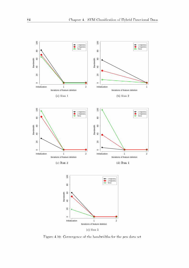
84 Chapter 4. SVM-Classi�cation of Hybrid Functional Data
020
4060
8010
0
Iterations of feature deletion
Ban
dwid
th
●
● ●
●
x trajectoryy trajectoryforce
Initialization 1 2
(a) Run 10
2040
6080
100
Iterations of feature deletion
Ban
dwid
th
●
●
●
x trajectoryy trajectoryforce
Initialization 1
(b) Run 2
020
4060
8010
0
Iterations of feature deletion
Ban
dwid
th
●
● ●
●
x trajectoryy trajectoryforce
Initialization 1 2
(c) Run 3
020
4060
8010
0
Iterations of feature deletion
Ban
dwid
th
●
● ●
●
x trajectoryy trajectoryforce
Initialization 1 2
(d) Run 4
020
4060
8010
0
Iterations of feature deletion
Ban
dwid
th
●
● ●
●
x trajectoryy trajectoryforce
Initialization 1 2
(e) Run 5
Figure 4.10: Convergence of the bandwidths for the pen data set

4.3. Numerical Experiments 85
●
●
● ● ● ●● ● ●
●●
●
●●
●
5060
7080
9010
0
C
Acc
urac
y (%
)
2−7 2−6 2−5 2−4 2−3 2−2 2−1 20 21 22 23 24 25 26 27
(a) Sensitivity analysis (C)
● ● ● ● ● ●
5060
7080
9010
0
δ
Acc
urac
y (%
)
10−10 10−9 10−8 10−7 10−6 10−5
(b) Sensitivity analysis (δ)
● ● ● ● ● ●
5060
7080
9010
0
iterations
Acc
urac
y (%
)
5 6 7 8 9 10
(c) Sensitivity analysis (number iterations)
Figure 4.11: Results of the sensitivity analysis for the retail data set
Trigonometric data set
Figure 4.14 shows that our proposal improves the performance of the comparative al-
gorithms.
With respect to the feature selection output, features one and three are selected
in the �ve runs, and variable two in three out of �ve. Indeed, the fourth run gives
ω = (0.3758, 0.1281, 0.0929, 0) as optimal solution.
Focusing on the sensitivity analysis with respect to δ and the number of iterations,
stability in the results is obtained. Nevertheless, the value of C has an important role
in the accuracy values, as seen in Figure 4.7.
The evolution of the values of the bandwidths in all the �ve runs is depicted in

86 Chapter 4. SVM-Classi�cation of Hybrid Functional Data
020
4060
8010
0
Iterations of feature deletion
Ban
dwid
th
●
● ●
●
AmountQuantityRecencyFrequencyMonetaryUK customer?
Initialization 1 2
(a) Run 10
2040
6080
100
Iterations of feature deletion
Ban
dwid
th
●● ●
●
AmountQuantityRecencyFrequencyMonetaryUK customer?
Initialization 1 2
(b) Run 2
020
4060
8010
0
Iterations of feature deletion
Ban
dwid
th
●
● ●
●
AmountQuantityRecencyFrequencyMonetaryUK customer?
Initialization 1 2
(c) Run 3
020
4060
8010
0
Iterations of feature deletion
Ban
dwid
th
●
● ●
●
AmountQuantityRecencyFrequencyMonetaryUK customer?
Initialization 1 2
(d) Run 4
020
4060
8010
0
Iterations of feature deletion
Ban
dwid
th
●
● ●
●
AmountQuantityRecencyFrequencyMonetaryUK customer?
Initialization 1 2
(e) Run 5
Figure 4.12: Convergence of the bandwidths for the retail data set

4.3. Numerical Experiments 87
●
●
● ●●
●
●●
alt f st dis r0 r1 r2 r3 r4 r5 r6 r7
5060
7080
9010
0
Acc
urac
y (%
)
Figure 4.13: Accuracy of batch data set in all the algorithms performed
Figure 4.8.
Pen data set
We conclude from Figure 4.15 that our methodology is comparable with the remaining
strategies. Moreover, we select just one variable out of three in two of the �ve runs.
The evolution of the bandwidths values can be seen in Figure 4.10.
In this example, the value of C is critical, as can be observed in Figure 4.9(a), since
the di�erence between the best and the worst case is around 40 points. However, our
method is robust with respect to δ and the number of iterations, as shown in Figures
4.9(b) and 4.9(c).
Retail data set
Figure 4.16 presents the accuracy boxplots of all the algorithms tested. We observe that
our proposal yields comparable results with the remaining methodologies. Moreover,

88 Chapter 4. SVM-Classi�cation of Hybrid Functional Data
●
●
●
●
alt f st dis r0 r1 r2 r3 r4 r5 r6 r7
5060
7080
9010
0
Acc
urac
y (%
)
Figure 4.14: Accuracy of trigonometric data set in all the algorithms performed
the selected variables are the third and sixth in four of �ve runs. As an illustration, the
optimal bandwidth in one of these runs is ω = (0, 0, 1.5887, 0, 0, 45.5919). Feature 3 and
Feature 6 correspond to Recency (number of months since the last purchase) computed
for each of the 10 months, and UK Customer (a binary variable that indicates whether
the customer comes from the UK). Since our objective is to predict whether a customer
will buy products or not in the last three months, it seems that it is important to know
the elapsed number of months since the last purchase. In addition, we observe that the
customer origin plays an important role; customers in the UK tend to buy less than
foreign customers.
Similar conclusions to the ones shown in the rest of the examples can be stated with
respect to the sensitivity analysis.
In this example, it is even more clear that the choice of the parameter C is a crucial
issue for obtaining good accuracy, as seen in Figure 4.11(a).
Figures 4.11(b) and 4.11(c) show again that the elimination threshold δ and the
number of iterations do not a�ect the e�ectiveness of our approach.

4.4. Conclusions and Extensions 89
●
alt f st dis r0 r1 r2 r3 r4 r5 r6 r7
5060
7080
9010
0
Acc
urac
y (%
)
Figure 4.15: Accuracy of pen data set in all the algorithms performed
In Figure 4.12 we can observe the evolution of the values of the di�erent bandwidths,
converging in a small number of iterations.
4.4 Conclusions and Extensions
In this chapter, we have shown how a feature selection strategy can be embedded in the
well-known SVM technique to get the most informative covariates of hybrid functional
data.
To do this, we have modi�ed the standard Gaussian kernel by associating a band-
width to each variable. Such bandwidths and the rest of the SVM parameters are
sought via a bilevel optimization problem solved with an alternating approach. Instead
of minimizing the misclassi�cation rate, we propose to maximize the Pearson correlation
coe�cient between the class label and the score. Other measures such as the correlation
in [Torrecilla Noguerales, 2015] can also be applied.
A sensitivity analysis of the setting parameters involved in our approach was made
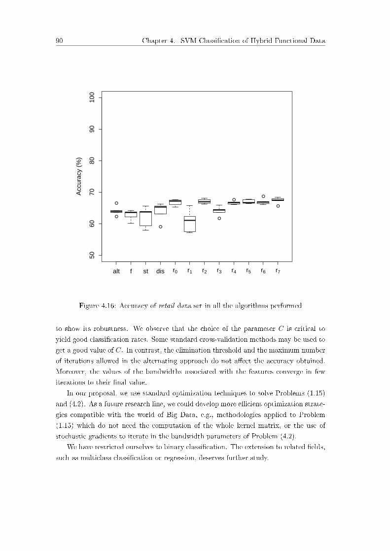
90 Chapter 4. SVM-Classi�cation of Hybrid Functional Data
●
●
●
●
●●
●
alt f st dis r0 r1 r2 r3 r4 r5 r6 r7
5060
7080
9010
0
Acc
urac
y (%
)
Figure 4.16: Accuracy of retail data set in all the algorithms performed
to show its robustness. We observe that the choice of the parameter C is critical to
yield good classi�cation rates. Some standard cross-validation methods may be used to
get a good value of C. In contrast, the elimination threshold and the maximum number
of iterations allowed in the alternating approach do not a�ect the accuracy obtained.
Moreover, the values of the bandwidths associated with the features converge in few
iterations to their �nal value.
In our proposal, we use standard optimization techniques to solve Problems (1.15)
and (4.2). As a future research line, we could develop more e�cient optimization strate-
gies compatible with the world of Big Data, e.g., methodologies applied to Problem
(1.15) which do not need the computation of the whole kernel matrix, or the use of
stochastic gradients to iterate in the bandwidth parameters of Problem (4.2).
We have restricted ourselves to binary classi�cation. The extension to related �elds,
such as multiclass classi�cation or regression, deserves further study.

Chapter 5
SVR with Functional Data
91


5.1. Introduction 93
5.1 Introduction
In contrast to what is analyzed in previous chapters, in this chapter we focus on func-
tional regression, [Ferraty et al., 2010; Hernández et al., 2007; James et al., 2009; Kneip
et al., 2016; Müller and Stadtmüller, 2005], one of the most challenging problems in
FDA. Particularly, we are interested in the prediction of a scalar response, based on the
information provided by multivariate functional data.
Predictor-response relationships are harder to be found and interpret as the di-
mension of the data becomes larger, or even in�nite, as in our case. Selecting from
the whole time interval a �nite and small set of time instants can be understood as
a variable selection strategy from an in�nite set of features, which may lead to better
predictions.
Several works in the literature have addressed the problem of variable selection in
univariate functional data, as is outlined in Section 1.3. However, with respect to the
variable selection in multivariate regression with functional data, scarce methodologies
has been reported in the literature. We can just highlight the work in [Blanquero et al.,
2017] for classi�cation problems, based on Chapter 2 of this dissertation.
Hence, the problem of optimal selection of time instants in (multivariate) functional
regression, as addressed in this chapter, is new in the literature. More precisely, we focus
on SVR, a renowned methodology for regression problems, that allows us to capture
nonlinearities. We stress the importance of developing a methodology able to handle
multivariate functional data; �rst of all, on top of making the approach applicable to
many more contexts, one can always associate with each functional data the function
itself, as well as the functional data of its derivatives, allowing to use information on the
data values as well as information related to monotonicity or convexity, for instance, as
done in Chapter 2. Taking advantage of the functional behavior of the data, the selected
features act as continuous decision variables in the optimization model. Therefore, the
so-obtained optimization problem may be solved by means of continuous optimization
techniques. If instead, the data were treated as multivariate �nite-dimensional data,
combinatorial problems, very hard to solve due to the exponential number of candidate
solutions, would have been obtained. Furthermore, following the scheme of Chapter 2,
our proposal handles in the very same way univariate and multivariate functions.
The remainder of this chapter is structured as follows. In Section 5.2, we detail the
formulation and the solution approach, as well as the way to choose the best number
of time points. Section 5.3 describes the numerical results obtained with our approach
and we �nish in Section 5.4 with some conclusions.
94 Chapter 5. SVR with Functional Data
5.2 The Variable Selection Problem
Section 5.2.1 is devoted to introduce the main concepts and notation used in the time
instant selection problem. In Section 5.2.2 the problem of variable selection in SVR
with functional data is formulated, and a resolution strategy is proposed.
5.2.1 Preliminaries
As denoted along this dissertation, let s be a sample of individuals {(Xi, Yi)}i∈s, whereYi ∈ R and Xi ∈ X = Fp is formed by p functional components, as in Equation (1.1)
with Xiv : [0, T ] → R belonging to the class F of d-times continuously di�erentiable
functions on the time interval [0, T ]. The goal is to �nd a rule able to predict the
response Y ∈ R from the information provided by the multivariate functional data
X ∈ X .Our proposal can be applied to pure multivariate functional data, but also on uni-
variate functional data, X(t) ∈ F . The simplest way to do that would be just to
consider p = 1. However, a more sophisticated form is applied, in which univariate data
can be converted to multivariate by means of their derivatives, as done in Equation
(2.2). Using the very same strategy, the high-order information provided by the deriva-
tives can be also included in the pure multivariate functional data, X(t) ∈ Fp, yieldingdata of the form (2.3).
In many real-life applications, the original functional data Xi are only known in
some time instants. Hence, smoothing techniques, e.g., [De Boor, 1978; Friedman et al.,
2001b], should be applied as a preprocessing step in those cases, so that an approxima-
tion to the original function Xi can be obtained from the observed time instants.
Moreover, if the higher-order information is taken into account, one can �rst compute
the �nite increments, and then smooth the sequence of increments. An example of the
�rst derivative of X(t) in the discretization point th is given in (2.4). This process
should be repeated for all the instants th in the discretized function and for any higher-
order derivative. Such discretized derivatives will be then smoothed with some of the
previously mentioned interpolation techniques.
5.2.2 Problem Formulation
The aim of this chapter is to �nd time instants t1, . . . , tH in such a way that the
relationship between the functional predictor X and the scalar response Y , obtained
via the SVR problem in (1.17), is as good as possible, in some sense to be speci�ed.
Two very di�erent types of parameters can be found in the variable selection pro-
blem. First, the H time instants t = (t1, . . . , tH) satisfying that 0 ≤ t1 ≤ . . . ≤ tH ≤ T ,and second, the parameters ε, C, ω involved in the SVR problem (1.17), and in the
Gaussian kernel (1.27), respectively.

5.2. The Variable Selection Problem 95
Following the strategy of Chapters 2, 3 and 4, we propose to �nd the optimal param-
eters ε, C, ω, t, by combining a grid search for the parameter ε, and the resolution of
a bilevel optimization problem for the remaining parameters. This bilevel optimization
problem aims at minimizing the performance measure given by the sum of the squared
residuals (SSR) between the real response value Yi and the score Y (Xi(t), C,ω, ν, ν∗)
in (1.18).
In order to obtain more stable results and avoid over�tting, we proceed as in previous
chapters, and we divide the sample s into four independent samples, s1, s2, s3 and s4 as
follows. We �rst divide the sample into k folds. Then, k−1 folds are randomly selected
and divided into three parts, yielding samples s1, s2 and s3. The remaining fold forms
sample s4. Samples s1 and s2 play the role of training samples, whilst s3 and s4 are
the validation and testing samples, respectively. Particularly, the independent sample
s1 is used to obtain the optimal values of ν and ν∗ by solving Problem (1.17) for �xed
C, ω, t and ε. Sample s2 is employed to compute the residuals between the response
Yi and the score Y (Xi(t), C,ω, ν, ν∗). Sample s3 is utilized to tune the parameter ε by
evaluating the performance measure SSR for all the values in the grid, and keeping the
parameter yielding the smallest residual. Finally, sample s4 is used to estimate the SSR
and test the �nal results.
Hence, for a given ε, the bilevel optimization problem is stated as follows:
minC,ω,t,ν,ν∗
∑i∈s2
(Yi − Y (Xi(t), C,ω, ν, ν∗))2
s.t. ν, ν∗ solves (1.17) in s1,
C ≥ 0,
ωv ≥ 0, v = 1, . . . , p
0 ≤ t1 ≤ . . . ≤ tH ≤ T
(5.1)
Problem (5.1) can be handled with an alternating algorithm, as also done in Chapters
2, 3 and 4. In the �rst step of our alternating procedure, Problem (1.17) is solved in
sample s1 for given C,ω and t, obtaining the optimal SVR variables ν and ν∗. Problem
(1.17) is a quadratic concave maximization problem with linear constraints. Hence,
classic local search routines may be applied to �nd the global optimum. In the second
step, for ν and ν∗ �xed, we get the optimal C,ω and t solving Problem (5.2) in sample
s2. Problem (5.2) is a continuous optimization problem which is solved by combining
standard local searches with a multi-start strategy to avoid getting stuck at bad local
optima.

96 Chapter 5. SVR with Functional Data
minC,ω,t
∑i∈s2
(Yi − Y (Xi(t), C,ω))2
s.t. C ≥ 0,
ωv ≥ 0, v = 1, . . . , p
0 ≤ t1 ≤ . . . ≤ tH ≤ T
(5.2)
The alternating approach is run, for a �xed ε, until some stopping criteria is met,
yielding good values of C,ω, t, ν and ν∗. The value of ε is obtained with a grid search,
i.e., computing, for each ε in the grid, the performance measure SSR on the sample s3,
and keeping the one with the smallest value.
Finally, to test the e�ciency of our approach, we calculate the SSR in a fourth
independent sample s4.
The pseudocode of our proposal can be seen in Algorithm 6.
Algorithm 6 Heuristic for variable selection
Input: H.• Randomly split the sample s into s1, s2, s3 and s4.• Compute the derivatives of the functional data.• Smooth the data with some interpolation technique.for ε in the grid do
Alternating Procedurerepeat
1. For C,ω, t �xed, calculate the parameters ν, ν∗ of the SVR problem (1.17)using the sample s1.
2. Fixed ν and ν∗ �xed, compute C,ω, t by solving Problem (5.2)sample s2.
until stopping criteria• Evaluate the performance measure SSR using the sample s3 for the ε �xed inthe grid.
end for• The optimal value of ε is the one with minimum performance measure SSR in s3,and the optimal values of ν, ν∗, C, ω and t are the parameters associated to theoptimal ε.Output: Optimal parameters ε, C,ω, t, ν, ν∗, and the performance measure SSRestimated on s4.
In order to enhance the performance of the heuristic, we propose to de�ne, as in
Chapters 2 and 3, a series of nested models of increasing complexity, in which the
optimal solution of a simple model is employed as initial solution in a more complex
case. In other words, when seeking the h + 1 time instants in th+1, one considers as
initial solution a perturbation of th, i.e., the optimal solution obtained when only h
time instants are sought. Therefore, if we want to �nd the H time instants that best
predict, we consider the easy-to-tune structure of the simple cases as a simpli�cation
of the complex models, in such a way that the (suboptimal) solution K(Xi, Xj ,ωh, th)

5.3. Numerical Experiments 97
is used as initial solution for kernel K(Xi, Xj ,ωh+1, th+1). More speci�cally, the initial
solution of the parameters C and ω in the level h + 1 are set as the optimal values
of such parameters in the level h, ωhopt and Chopt, respectively. Moreover, the choice of
the initial solution of the h + 1 time instants in th+1 is made by selecting a random
value τ ∈ [0, T ], and including it in the appropriate position of the optimal solution of
the level h, thopt. In other words, th+1opt = σ(τ, thopt), where σ is a function that sorts in
increasing order the time instants thopt and τ .
The pseudocode of the nested heuristic is outlined in Algorithm 7.
Observe that our proposed heuristic di�ers from a greedy approach [Berrendero et
al., 2018; Ferraty et al., 2010], since our proposal utilizes the optimal solution of level
h just as starting solution of the level h+ 1, allowing a very di�erent solution for level
h+ 1 than the one obtained in the previous level, h. Consequently, our approach gives
more �exibility to the model.
Moreover, when the exact number of selected time instants, H, is unknown, our
algorithm has the advantage of allowing us to build a trajectory of the performance
measure SSR in terms of the number of time instants. It may be very useful when a
list of models with di�erent complexity is needed.
5.3 Numerical Experiments
This section is devoted to the computational experience on the proposed models. In
Section 5.3.1 we describe the experiments performed. Section 5.3.2 details the data sets
used to test our methodology, and Section 5.3.3 analyses the numerical results.
5.3.1 Description of the Experiments
Algorithm 7 is run to show the usefulness of our approach, i.e., to test whether the
predictions obtained when H time instants are carefully chosen are comparable, or even
better, to the residuals achieved when the full time interval is considered.
To get stable results, k−fold cross-validation is accomplished. The number k of
folds is dependent on the data set. More precisely, if a database is big, then k = 10 is
chosen. By contrast, in the small data sets leave-one-out is performed, i.e., k coincides
with the number of observations. Here, we consider that a database is big if it has more
than 100 observations. More details about the cardinality of the databases can be seen
in Table 5.1. Algorithm 7 is run k times, one per fold. In each run, the data set is split
into four parts, s1−s4, as described in Section 5.2.2. As the output of our methodology,
we provide the average SSR estimated on the test sample s4 over all the folds.
The number of runs in the multi-start is �ve. The Alternating Procedure is stopped
either when ten iterations are executed or when the di�erence between the objec-
tive values of two consecutive iterations is lower than 10−5. The maximum num-

98 Chapter 5. SVR with Functional Data
Algorithm 7 Nested heuristic for variable selection
Input: H, nested kernels K(Xi, Xj ,ω1, t1) ≺ . . . ≺ K(Xi, Xj ,ω
H , tH).• Randomly split the sample s into s1, s2, s3 and s4.• Compute the derivatives of the functional data.• Smooth the data with some interpolation technique.for ε in the grid do
Initialization:• h := 1.• Randomly select an initial solution C1 ∈ [0,+∞), ω1 ∈ [0,+∞)p andt1 := t1 ∈ [0, T ].• Set (C,ω, t) := (C1, ω1, t1).while h ≤ H do
1. Run the Alternating Procedure of Algorithm 6 for K(Xi, Xj ,ωh, th),
starting from (C,ω, t) and yielding (Chopt,ωhopt, t
hopt) as solution, using
samples s1 and s2.2. Randomly generate τ ∈ [0, T ].3. Set Ch+1 := Chopt, ω
h+1 := ωhopt, th+1 := σ(τ, thopt),
(C,ω, t) := (Ch+1,ωh+1, th+1) and h := h+ 1.4. Evaluate the performance measure SSR over the sample s3 with ε �xed.
end whileend for• For each h, the optimal value of ε is the one with the minimum performance measureSSR in s3. The optimal values of ν, ν∗, C, ω and t are the parameters associated tothe optimal ε.Output: Optimal parameters Chopt, ω
hopt, t
hopt, ∀h, the associated coe�cients ε, ν, ν∗,
and the performance measure SSR estimated from s4.
ber of time instants to be sought is H = 20, and the parameter ε moves in the set
{10−4, 10−3, 10−2, 10−1}.All the experiments were carried out on a cluster with 2 Tb of RAM memory at 6.2
TFlops, running CentOS Linux 7.3, and it is coded in R, [Core Team, 2017].
5.3.2 Description of the Data Sets
We have tested our proposal on six univariate and two multivariate databases, widely
used in the literature on functional regression. The univariate databases are denoted
as canadian, [Goldsmith and Scheipl, 2014; James et al., 2009], cookie, [Goldsmith and
Scheipl, 2014], DTI, [Goldsmith and Scheipl, 2014], simulated, [Ferraty et al., 2010],
sugar, [Aneiros and Vieu, 2014], and tecator, [Ferraty et al., 2010; Goldsmith and
Scheipl, 2014; Picheny et al., 2018]. Multivariate databases are named as synthetic_1
and synthetic_2 and come from [Matsui and Konishi, 2011]; both of them have the
same independent variables and only di�er in the response variable. A sample of ten
individuals of all the univariate databases is given in Figure 5.1. A sample of the obser-
vations of the dataset synthetic_1 (and synthetic_2 ) is depicted in Figure 5.2. Table

5.3. Numerical Experiments 99
5.1 gives a summarized description of the data sets, including the number of records,
the number of time instants where data are discretized, and the number of covariates.
#records #time instants #componentscanadian 35 365 1cookie 72 700 1DTI 334 93 1
simulated 1500 100 1sugar 268 571 1
synthetic_1 300 101 3synthetic_2 300 101 3
tecator 215 100 1
Table 5.1: Data description summary
Details about each data set are presented in the following lines.
Canadian Data Set
The canadian data set have been studied in e.g., [Goldsmith and Scheipl, 2014; James
et al., 2009]. The explanatory variables are formed by the daily temperature along one
year measured on 35 Canadian weather stations, as in the rain and regions data set of
Section 2.3.2. However, in this chapter the goal is to predict the logarithm of the total
annual rainfall.
Cookie Data Set
This database can be found in [Goldsmith and Scheipl, 2014] and measures the 72
spectra of cookie dough samples every two nanometers (nm) from 1,100 to 2,498 nm
with the aim of predict the percentage of sucrose content.
DTI Data Set
The DTI data set, [Goldsmith and Scheipl, 2014], consists of 334 observations that
measure in 93 points the white matter in the corpus callosum to predict the cognitive
performance in order to study multiple sclerosis lesions.
Simulated Data Set
According to the example of Section 3.2 of [Ferraty et al., 2010] we have generated
1,500 curves discretized in 100 equispaced points in the interval [0, 2π] following this

100 Chapter 5. SVR with Functional Data
structure:
Xi(t) =
3∑`=1
Ui` cos{(3 + `)t}+
3∑`=1
Vi` sin{(4 + `)t}+Wi(t− π)2, i = 1, . . . , 1, 500
where Ui`, Vi`, Wi, ` = 1, 2, ∀i are uniformly distributed in [0, 1], whereas Ui3 and
Vi3 follow a normal distribution N (0, 0.25), where the second parameter denotes its
variance.
For i = 1, . . . , 1, 500, the values of the response variable are obtained from the model
Yi = r(Xi) + γi, based on the time instants t ∈{
48π99 ,
58π99 ,
128π99
}with
r(Xi) = Xi
(48π
99
)+ 2Xi
(58π
99
)Xi
(128π
99
), (5.3)
and γi independent and identically distributed as N (0, σ2γ), with σ2
γ = 5% var{r(Xi)}.
Sugar Data Set
The goal of this data set from [Aneiros and Vieu, 2014] is to predict the percentage of
ash content from the �uorescence spectra, measured on 571 points of 268 samples of
sugar.
Tecator Data Set
This data set deals with the near-infrared absorbance spectra of 215 samples of �nely
chopped pork, measured at 100 equally spaced points from 850 to 1,050 nanometers. It
has been previously used in Sections 2.3.2 and 3.4.2. Nevertheless, in this chapter, the
response variable represents the fat content. More details can be found in [Ferraty et
al., 2010; Goldsmith and Scheipl, 2014; Picheny et al., 2018].
Synthetic_1 and Synthetic_2 Data Sets
In this section we have dealt with 300 observations of two data sets, namely synthetic_1
and synthetic_2, generated as in [Matsui and Konishi, 2011]. The three predictor
variables are built as follows, for t ∈ [−1, 1]:
Xv(t) = Uv(t) + γv, v = 1, 2, 3, (5.4)

5.3. Numerical Experiments 101
where γv ∼ N (0, 0.025 · (rv)2) and rv = maxt
(Uv(t))−mint
(Uv(t)). Furthermore,
U1(t) = cos(2π(t− a1)) + a2t; a1 ∼ N (−5, 32); a2 ∼ N (7, 1)
U2(t) = b1 sin(2t) + b2; b1 ∼ U(3, 7); b2 ∼ N (0, 1)
U3(t) = c1t3 + c2t
2 + c3t+ c4; c1 ∼ N (−3, 1.22); c2 ∼ N (2, 0.52); c3 ∼ N (−2, 1); c4 ∼ N (2, 1.52)
The response variable Y is given by:
Y = g(U) + ν0 (5.5)
with
g(U) =
3∑v=1
∫ 1−1 Uv(t)ϕv(t)dt; ν0 ∼ N (0, (c · s)2); s = max(g(U))−min(g(U))
ϕ1(t) = sin(2πt); ϕ2(t) = sin(πt); ϕ3(t) = 0
(5.6)
The value c of the parameter ν0 in (5.6) depends on the multivariate data set. More
precisely, c = 0.05 in the database synthetic_1 and c = 0.1 in synthetic_2.
5.3.3 Results
Figure 5.3 shows the trajectory of the SSR obtained when H time instants are sought,
ranging from H = 1 to H = 20. We depict in dotted-red, triangled-blue and crossed-
green solid lines the results when d = 0, 1, 2 derivatives are considered, respectively.
To test the performance of our methodology, we use the maximum and minimum
SSR values from a set of benchmark procedures in the literature. We indicate the
reference SSR values in the cases where they are available, i.e., in data sets simulated,
sugar and tecator by depicting them in solid black line (maximum residual), and dashed
pink line (minimum residual). More precisely, the benchmark values come from [Ferraty
et al., 2010] in simulated and tecator ; and from [Aneiros and Vieu, 2014] in sugar.
Moreover, in the cases where such reference values are not available, we compare our
proposal with the SSR obtained when the full time domain is taking into account.
Indeed, we have run Algorithm 7 with the same settings of Section 5.3.1, i.e., number
of iterations, stopping criterion, and values of the parameter ε, to get the variables
ν, ν∗, C and ω of Problem (5.1) together with the average of performance measure SSR
across folds on exactly the same testing sample s4, where variable selection is performed.
The results of Algorithm 7 when no variable selection is performed, i.e., the full (time)
domain is taken into account, are plotted on dotted red, blue or green line depending
if the degree of the derivatives is d = 0, 1 or 2, respectively. In addition, some parts of
the output �gures of the databases simulated, synthetic_1 and tecator are zoomed in
order to improve the visualization.

102 Chapter 5. SVR with Functional Data
On top of that, we will show that high-order information is crucial to achieving good
residual values. Hence, Algorithm 7 is run for three di�erent values of the derivatives
d = 0, 1, 2, which include, respectively, the situations where just the information of the
raw functional data, or their monotonicity, or both their monotonicity and convexity
are considered. The exact values of all the SSR are given in Tables 5.2 and 5.3 for
comparison purposes.
In addition to the variable selection experiments, we also provide the best number
H of time instants, applying the same strategy as in Chapters 2 and 3.
As a general conclusion, looking at Figure 5.3 and Tables 5.2 and 5.3, we state
that the high-order information provided by the derivatives is crucial to get good pre-
dictions since most of the SSR obtained when monotonicity or both monotonicity and
convexity are taken into account are better than the values obtained just using the in-
formation of the functional data alone. Moreover, when we compare our approach with
the benchmarks in the literature, we conclude that SSR are improved with our method.
With respect to the best number of time instants, H, Figure 5.4 shows the boxplots
of the best time instants chosen when the number of time instants to be selected ranges
from H = 1 to H = 20.
On top of the overall conclusions given so far, more precise information on each data
set is given in the following lines.
Canadian Data Set
Figure 5.3(a) and Table 5.2 show the results obtained forn this data set applying our
methodology. Although there is not a clear pattern, possibly due to the small size of
the data set, we observe that, the larger the number of time instants used, the lower
the SSR, yielding in some cases better values when choosing appropriate time points
than when using the full domain information, e.g., d = 1 and H = 5.
Regarding the interpretability of the results, [James et al., 2009] a�rms that the
temperatures in the spring and fall months do have a noticeable e�ect when predicting
the annual rainfall. More speci�cally, Figure 4 of [James et al., 2009] shows that such
an e�ect is produced around the months of April and November. Figure 5.5 shows the
density histogram of the time instant values when H = 7 time points are sought using
our methodology. We clearly observe that the majority of values are located around
the months of April and November independently of the value given to the parameter
d ∈ {0, 1, 2} exactly as is stated in [James et al., 2009]. Similar results are obtained
when H 6= 7, and therefore no more histogram �gures are plotted.

5.3. Numerical Experiments 103
Cookie Data Set
It is clear from Figure 5.3(b) and Table 5.2 that the derivative information plays a very
important role when seeking the most informative time instants, since the highest SSR
are obtained when only the raw data, and not the derivatives are used, i.e., when d = 0.
Furthermore, using only a few time instants yields better residuals than using the full
time interval, as can be seen, for instance for d = 1 and H = 4.
DTI Data Set
If we observe Figure 5.3(c) and Table 5.2, similar results were achieved with d = 0 and
H = 6 than when comparing with the full time domain and d = 0.
Simulated Data Set
Since the median of the SSR values is given as reference in [Ferraty et al., 2010], in this
example we give as output the median values instead of the mean, as the y−axis labelof Figure 5.3(d) indicates. Table 5.2 also shows the median values for this database.
On top of that, the response variable is constructed using the evaluation of the
predictor variable in three �xed time instants, namely 48π99 ,
58π99 and 128π
99 , as expressed
in (5.3). Because of this, we have also run Algorithm 7 with the settings given in
Section 5.3.1, and �xing such three time instants. The results are depicted in red, blue
and green dashed-dotted line for the d = 0, 1, 2 degrees derivatives, respectively.
In the zoomed plot of Figure 5.3(d), it is observed that similar results are obtained
with our methodology than with the minimum reference residual (pink dashed line) or
even better if the values with d = 0 are inspected.
Sugar Data Set
Figure 5.3(e) and Table 5.2 show that noticeable improvements in terms of SSR are
obtained with our approach, either compared with the SSR values reported in the
literature or with the model in which the full time interval is considered and no feature
selection is made. See the example of d = 2 and H = 3, for instance.
Tecator Data Set
Figure 5.3(h) and Table 5.2 show that our approach is able to improve the literature
reference values in [Ferraty et al., 2010], and is comparable to the results given when
the full interval is used and no feature selection is performed, especially if we compare
with d = 2.
104 Chapter 5. SVR with Functional Data
Synthetic_1 and Synthetic_2 Data Sets
We see in Figure 5.3(f), 5.3(g), and Table 5.3 that similar results in terms of prediction
ability have been obtained with and without feature selection. An example of this fact
is observed in the set synthetic_2 when d = 2, and H = 2.
5.4 Conclusions and Extensions
In this chapter, we have proposed an approach based on continuous optimization to
select time instants in regression problems with (multivariate) functional data.
The heuristic here proposed is enhanced with the de�nition of a nested structure
which takes advantage of the optimal solutions in the simple models to reach better pre-
dictions. Furthermore, our proposal allows, in the very same manner, to take advantage
of higher-order information provided by the derivatives of the (multivariate) functional
data. Such information is crucial, as has been shown in the numerical experience.
Some extensions of the present work are possible. Here we have just considered
pure (multivariate) functional data. Our proposal can be easily extended to the hybrid
multivariate case with a simple modi�cation of the kernel function, as in Chapter 4.
In this chapter, we have restricted ourselves to the time instant selection problem.
A possible extension would be to optimally select H time intervals, instead of H time
instants. Figure 5.6 shows the histograms of the extreme points when H = 2 time
intervals are sought in the canadian data set. We observe again that the most important
domains are around the months of April and November.
Another challenging extension of our approach consists of working with spatio-
temporal data, in which one seeks the most relevant time instants and locations, or
to extend our proposal to other Data Science problems, such as clustering.
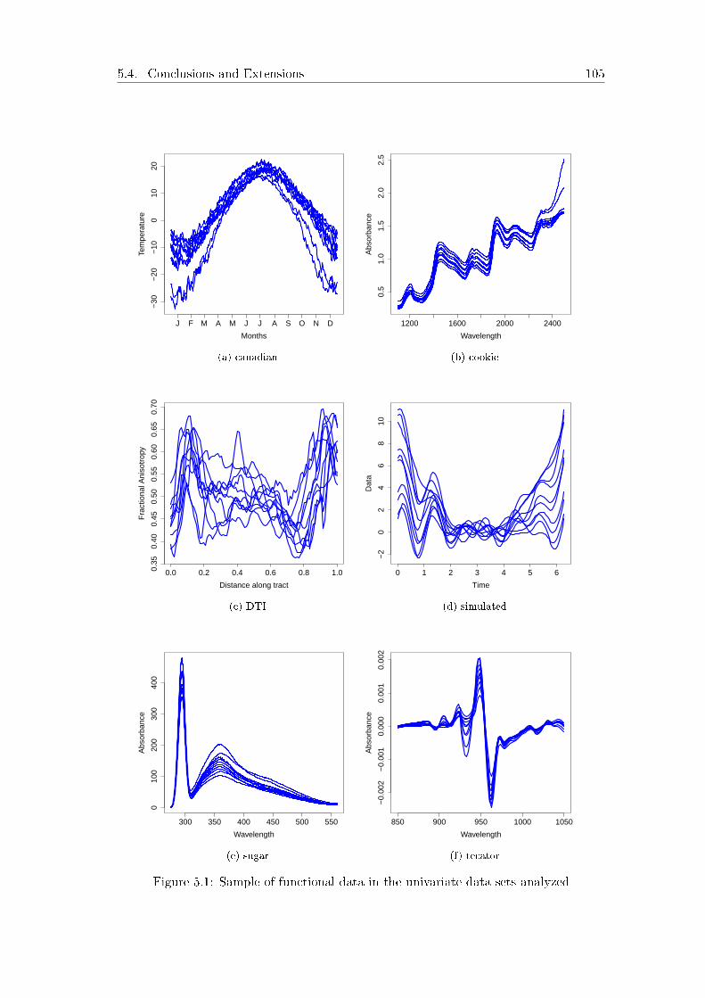
5.4. Conclusions and Extensions 105
−30
−20
−10
010
20
Months
Tem
pera
ture
J F M A M J J A S O N D
(a) canadian
1200 1600 2000 2400
0.5
1.0
1.5
2.0
2.5
Wavelength
Abs
orba
nce
(b) cookie
0.0 0.2 0.4 0.6 0.8 1.00.35
0.40
0.45
0.50
0.55
0.60
0.65
0.70
Distance along tract
Fra
ctio
nal A
niso
trop
y
(c) DTI
0 1 2 3 4 5 6
−2
02
46
810
Time
Dat
a
(d) simulated
300 350 400 450 500 550
010
020
030
040
0
Wavelength
Abs
orba
nce
(e) sugar
850 900 950 1000 1050
−0.
002
−0.
001
0.00
00.
001
0.00
2
Wavelength
Abs
orba
nce
(f) tecator
Figure 5.1: Sample of functional data in the univariate data sets analyzed
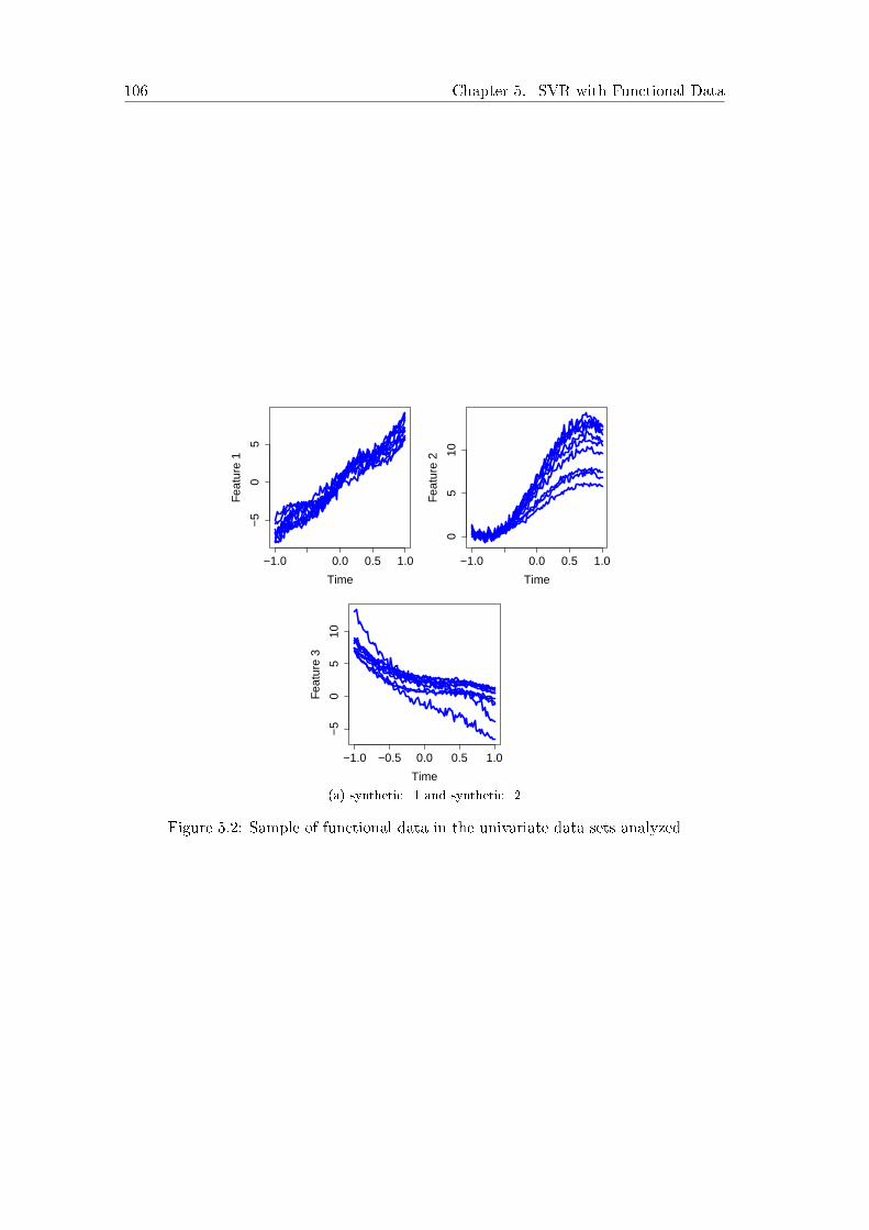
106 Chapter 5. SVR with Functional Data
−1.0 0.0 0.5 1.0
−5
05
Time
Fea
ture
1
−1.0 0.0 0.5 1.0
05
10
Time
Fea
ture
2
−1.0 −0.5 0.0 0.5 1.0
−5
05
10
Time
Fea
ture
3
(a) synthetic_1 and synthetic_2
Figure 5.2: Sample of functional data in the univariate data sets analyzed

5.4. Conclusions and Extensions 107
canadian
dfulldomain
H1
23
45
67
89
10
11
12
13
14
15
16
17
18
19
20
00.22
0.36
0.32
0.35
0.28
0.24
0.25
0.23
0.28
0.24
0.30
0.16
0.15
0.15
0.21
0.19
0.17
0.17
0.19
0.20
0.20
10.24
0.35
0.24
0.40
0.33
0.20
0.25
0.18
0.22
0.20
0.23
0.26
0.28
0.26
0.22
0.28
0.31
0.31
0.26
0.21
0.28
20.23
0.41
0.34
0.30
0.37
0.22
0.25
0.18
0.27
0.21
0.21
0.23
0.22
0.25
0.22
0.21
0.21
0.22
0.21
0.24
0.23
cookie
dfulldomain
H1
23
45
67
89
10
11
12
13
14
15
16
17
18
19
20
00.15
0.36
0.36
0.39
0.38
0.27
0.24
0.24
0.27
0.24
0.27
0.26
0.22
0.26
0.28
0.26
0.26
0.26
0.26
0.25
0.24
10.08
0.18
0.08
0.07
0.06
0.08
0.10
0.07
0.05
0.06
0.07
0.06
0.08
0.06
0.08
0.06
0.06
0.06
0.07
0.08
0.07
20.07
0.13
0.11
0.13
0.08
0.08
0.11
0.10
0.07
0.07
0.09
0.05
0.07
0.07
0.07
0.07
0.06
0.07
0.07
0.06
0.06
DTI
dfulldomain
H1
23
45
67
89
10
11
12
13
14
15
16
17
18
19
20
05.92
6.05
6.42
6.05
6.14
5.98
5.91
5.99
6.00
5.98
6.10
5.97
6.00
6.06
5.97
5.98
6.03
6.01
6.04
6.07
6.12
15.57
7.00
7.01
6.30
6.37
6.50
6.46
6.31
6.23
6.18
6.23
6.16
6.11
6.22
6.17
6.13
6.18
6.18
6.07
6.12
6.09
25.52
6.88
6.62
6.53
6.62
6.53
6.35
6.35
6.31
6.34
6.45
6.56
6.61
6.61
6.48
6.49
6.51
6.55
6.66
6.69
6.45
simulated
resmin
resmaxd
fulldomain
�xed
timeinstants
H1
23
45
67
89
10
11
12
13
14
15
16
17
18
19
20
0.16
0.82
00.12
0.07
9.40
4.73
1.10
0.91
0.29
0.20
0.15
0.11
0.11
0.12
0.12
0.12
0.12
0.12
0.12
0.12
0.12
0.11
0.11
0.11
10.18
0.09
10.23
6.26
0.62
0.20
0.18
0.20
0.22
0.20
0.20
0.21
0.22
0.21
0.21
0.21
0.20
0.21
0.21
0.20
0.20
0.19
20.25
0.19
10.97
0.98
0.33
0.24
0.23
0.25
0.25
0.25
0.26
0.27
0.26
0.25
0.26
0.26
0.25
0.24
0.25
0.26
0.26
0.26
sugar
resmin
resmaxd
fulldomain
H1
23
45
67
89
10
11
12
13
14
15
16
17
18
19
20
2.32
2.68
01.61
2.57
2.13
1.99
1.79
1.85
1.65
1.51
1.43
1.56
1.87
1.69
1.71
1.72
1.57
1.55
1.54
1.56
1.47
1.46
1.49
11.62
2.31
2.17
2.05
1.95
2.02
2.05
1.94
1.75
2.06
1.92
1.62
1.75
1.74
1.71
1.74
1.76
1.78
1.77
1.77
1.76
21.79
2.12
2.00
1.61
1.86
1.73
1.85
1.82
1.89
1.77
1.90
1.88
1.79
1.86
1.83
1.84
1.83
1.83
1.82
1.81
1.81
tecator
resmin
resmaxd
fulldomain
H1
23
45
67
89
10
11
12
13
14
15
16
17
18
19
20
0.7
8.8
00.03
0.80
0.19
0.16
0.14
0.10
0.12
0.09
0.11
0.09
0.09
0.08
0.09
0.06
0.05
0.05
0.03
0.04
0.05
0.05
0.05
10.02
0.51
0.23
0.12
0.10
0.07
0.05
0.05
0.06
0.05
0.06
0.05
0.05
0.04
0.04
0.03
0.04
0.04
0.04
0.04
0.04
20.04
0.54
0.16
0.13
0.07
0.05
0.04
0.05
0.06
0.06
0.06
0.06
0.04
0.04
0.05
0.03
0.03
0.04
0.05
0.06
0.05
Table5.2:
Perform
ance
resultson
univariate
data
sets
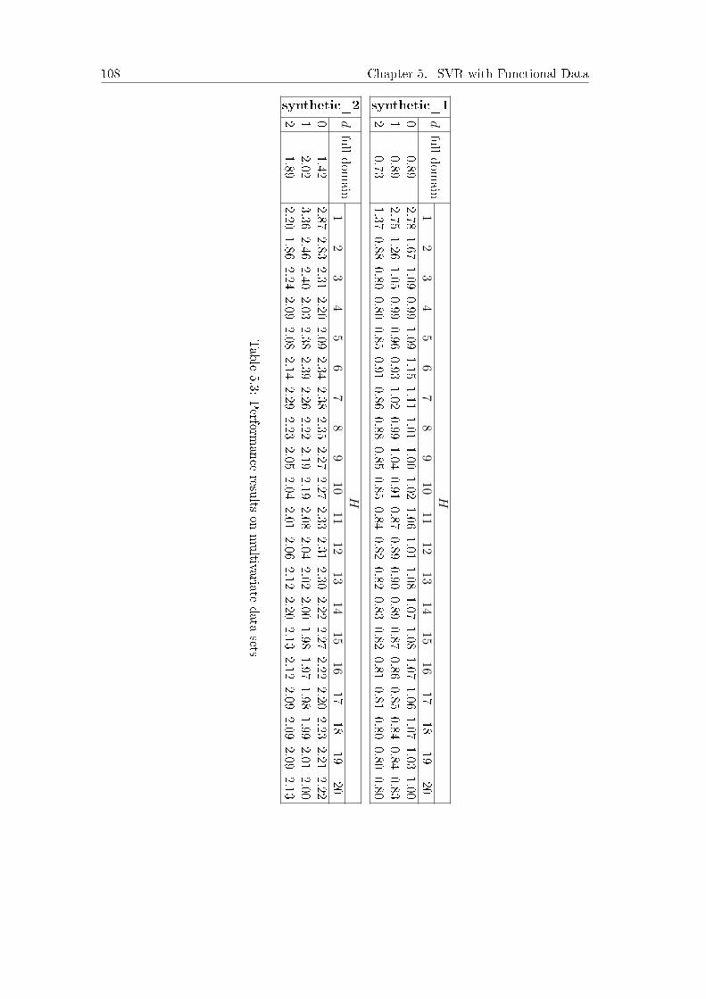
108 Chapter 5. SVR with Functional Data
synthetic_1
dfull
domain
H1
23
45
67
89
1011
1213
1415
1617
1819
200
0.892.78
1.671.09
0.991.09
1.151.11
1.011.00
1.021.06
1.011.08
1.071.08
1.071.06
1.071.03
1.001
0.892.75
1.261.05
0.990.96
0.931.02
0.991.04
0.910.87
0.890.90
0.890.87
0.860.85
0.840.84
0.832
0.731.37
0.880.80
0.800.85
0.910.86
0.880.85
0.850.84
0.820.82
0.830.82
0.810.81
0.800.80
0.80
synthetic_2
dfull
domain
H1
23
45
67
89
1011
1213
1415
1617
1819
200
1.422.87
2.832.31
2.202.09
2.342.38
2.352.27
2.272.33
2.312.30
2.222.27
2.222.20
2.232.21
2.221
2.023.36
2.462.40
2.032.38
2.392.26
2.222.19
2.192.08
2.042.02
2.001.98
1.971.98
1.992.01
2.002
1.892.20
1.862.24
2.092.08
2.142.29
2.232.05
2.042.01
2.062.12
2.202.13
2.122.09
2.092.09
2.13
Table
5.3:Perform
anceresults
onmultivariate
datasets

5.4. Conclusions and Extensions 109
●
●
●
●
●
●
●
●
●
●
●●
●
●
●
●●
●
●●
0.15
0.20
0.25
0.30
0.35
0.40
Number of time instants
Mea
n re
sidu
als
1 2 3 4 5 6 7 8 9 10 12 14 16 18 20
● d 0d 1d 2fd d 0fd d 1fd d 2
(a) canadian
● ●
●
●
●
●●
●
●
●
●
●
●
●
● ● ●●
●●
0.05
0.10
0.15
0.20
0.25
0.30
0.35
0.40
Number of time instants
Mea
n re
sidu
als
1 2 3 4 5 6 7 8 9 10 12 14 16 18 20
● d 0d 1d 2fd d 0fd d 1fd d 2
(b) cookie
●
●
●
●
●
●
● ● ●
●
●●
●
● ●
● ●●
●
●
5.5
6.0
6.5
7.0
Number of time instants
Mea
n re
sidu
als
1 2 3 4 5 6 7 8 9 10 12 14 16 18 20
● d 0d 1d 2fd d 0fd d 1fd d 2
(c) DTI
●
●
●●
● ● ● ● ● ● ● ● ● ● ● ● ● ● ● ●02
46
810
Number of time instants
Med
ian
resi
dual
s
1 2 3 4 5 6 7 8 9 10 12 14 16 18 20
● d 0d 1d 2res max res minfd d 0fd d 1fd d 2fti d 0fti d 1fti d 2
●
●
●
● ●● ●
● ● ● ● ● ● ● ● ●
0.05
0.15
0.25
0.35
3 5 7 9 11 14 17 20
(d) simulated
Figure 5.3: Variable selection results on databases canadian, cookie, DTI and simulated

110 Chapter 5. SVR with Functional Data
●
●
●
●
●
●
●
●
●
●
●● ●
●● ●
●
● ●●
1.4
1.6
1.8
2.0
2.2
2.4
2.6
Number of time instants
Mea
n re
sidu
als
1 2 3 4 5 6 7 8 9 10 12 14 16 18 20
● d 0d 1d 2res max res minfd d 0fd d 1fd d 2
(e) sugar
●
●
●
●
●
●●
● ●●
●●
● ● ● ● ● ●●
●1.
01.
52.
02.
5
Number of time instants
Mea
n re
sidu
als
1 2 3 4 5 6 7 8 9 10 12 14 16 18 20
● d 0d 1d 2fd d 0fd d 1fd d 2
0.89
00.
896
3 4
(f) synthetic_1
●●
●
●
●
●●
●
● ●
● ● ●
● ● ● ●● ● ●
1.5
2.0
2.5
3.0
Number of time instants
Mea
n re
sidu
als
1 2 3 4 5 6 7 8 9 10 12 14 16 18 20
● d 0d 1d 2fd d 0fd d 1fd d 2
(g) synthetic_2
●
● ● ● ● ● ● ● ● ● ● ● ● ● ● ● ● ● ● ●02
46
8
Number of time instants
Mea
n re
sidu
als
1 2 3 4 5 6 7 8 9 10 12 14 16 18 20
● d 0d 1d 2res max res minfd d 0fd d 1fd d 2
●
●
●
●
●
●
●
● ● ●●
●● ●
●●
● ● ●
0.00
0.05
0.10
0.15
0.20
0.25
2 4 6 8 10 12 14 16 18 20
(h) tecator
Figure 5.3: Variable selection results on databases sugar, synthetic_1, synthetic_2 andtecator (cont.)

5.4. Conclusions and Extensions 111
●
● ●
●
1
2
3
4
5
6
7
8
9
10
11
12
13
14
15
16
17
18
19
20
1 2 3 4 5 6 7 8 9 10 11 12 13 14 15 16 17 18 19 20
Maximum number of time instants
Opt
imal
num
ber
of ti
me
inst
ants
Derivatives
0
1
2
(a) canadian
●●●●●●●●●●● ●●●●●●
●●
●●●
●●●
1
2
3
4
5
6
7
8
9
10
11
12
13
14
15
16
17
18
19
20
1 2 3 4 5 6 7 8 9 10 11 12 13 14 15 16 17 18 19 20
Maximum number of time instants
Opt
imal
num
ber
of ti
me
inst
ants
Derivatives
0
1
2
(b) cookie
● ● ● ● ●
●
●
●
●
●
●
●
●
●●
●● ● ●
1
2
3
4
5
6
7
8
9
10
11
12
13
14
15
16
17
18
19
20
1 2 3 4 5 6 7 8 9 10 11 12 13 14 15 16 17 18 19 20
Maximum number of time instants
Opt
imal
num
ber
of ti
me
inst
ants
Derivatives
0
1
2
(c) DTI
● ● ●
●
●
●
●
●
●
●
●
●
●
●
●
●
●
●
●
●
●
●
●
●
●
●
●
●
●
●
●
●
●
●●
●
● ●
●
● ●
1
2
3
4
5
6
7
8
9
10
11
12
13
14
15
16
17
18
19
20
1 2 3 4 5 6 7 8 9 10 11 12 13 14 15 16 17 18 19 20
Maximum number of time instants
Opt
imal
num
ber
of ti
me
inst
ants
Derivatives
0
1
2
(d) simulated
Figure 5.4: Best choice of H on databases canadian, cookie, DTI and simulated

112 Chapter 5. SVR with Functional Data
●
●
● ●
●●●●
●●
●
● ●
1
2
3
4
5
6
7
8
9
10
11
12
13
14
15
16
17
18
19
20
1 2 3 4 5 6 7 8 9 10 11 12 13 14 15 16 17 18 19 20
Maximum number of time instants
Opt
imal
num
ber
of ti
me
inst
ants
Derivatives
0
1
2
(e) sugar
●●
●●
●●●
1
2
3
4
5
6
7
8
9
10
11
12
13
14
15
16
17
18
19
20
1 2 3 4 5 6 7 8 9 10 11 12 13 14 15 16 17 18 19 20
Maximum number of time instants
Opt
imal
num
ber
of ti
me
inst
ants
Derivatives
0
1
2
(f) synthetic_1
●
●
●
●
●
●
● ●
●●●●
●●●●
●
●
●●
●
●
●●
● ●●● ●●
●
● ●
●
●
●
●
●
●
1
2
3
4
5
6
7
8
9
10
11
12
13
14
15
16
17
18
19
20
1 2 3 4 5 6 7 8 9 10 11 12 13 14 15 16 17 18 19 20
Maximum number of time instants
Opt
imal
num
ber
of ti
me
inst
ants
Derivatives
0
1
2
(g) synthetic_2
●
● ●
●
● ● ●
●
●
●
●
●● ●
●
●
●●
●
1
2
3
4
5
6
7
8
9
10
11
12
13
14
15
16
17
18
19
20
1 2 3 4 5 6 7 8 9 10 11 12 13 14 15 16 17 18 19 20
Maximum number of time instants
Opt
imal
num
ber
of ti
me
inst
ants
Derivatives
0
1
2
(h) tecator
Figure 5.4: Best choice of H on databases sugar, synthetic_1, synthetic_2 and tecator(cont.)
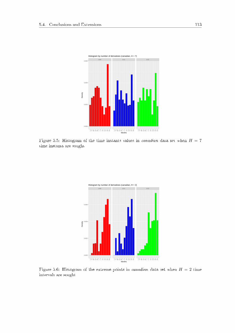
5.4. Conclusions and Extensions 113
d 0 d 1 d 2
J F M A M J J A S O N D J F M A M J J A S O N D J F M A M J J A S O N D
0.000
0.002
0.004
0.006
Months
Den
sity
Histogram by number of derivatives (canadian, H = 7)
Figure 5.5: Histogram of the time instants values in canadian data set when H = 7time instants are sought
d 0 d 1 d 2
J F M A M J J A S O N D J F M A M J J A S O N D J F M A M J J A S O N D
0.000
0.002
0.004
0.006
Months
Den
sity
Histogram by number of derivatives (canadian, H = 2)
Figure 5.6: Histogram of the extreme points in canadian data set when H = 2 timeintervals are sought


List of Figures
1.1 Two examples of functional data in real-life applications . . . . . . . . . 3
1.2 An example of multivariate functional data . . . . . . . . . . . . . . . . 6
1.3 An example of hybrid functional data . . . . . . . . . . . . . . . . . . . 7
2.1 Sample of functional data in the univariate data sets analyzed . . . . . . 33
2.2 Sample of functional data in the multivariate data sets analyzed . . . . . 35
2.3 Average accuracy in the univariate data sets analyzed . . . . . . . . . . . 37
2.4 Average accuracy in the multivariate data sets analyzed . . . . . . . . . 38
2.5 Boxplots of the optimal number of time instants in the univariate data sets 40
2.6 Boxplots of the optimal number of time instants in the multivariate data
sets . . . . . . . . . . . . . . . . . . . . . . . . . . . . . . . . . . . . . . . 44
3.1 regions data set . . . . . . . . . . . . . . . . . . . . . . . . . . . . . . . . 49
3.2 (a) and (b) show the bandwidth values for the regions data set when ω
has the form of (3.2) and (3.3), respectively . . . . . . . . . . . . . . . . 50
3.3 Time instant results for the regions data set with ω as in (3.3) . . . . . . 50
3.4 Sample of functional data in the data sets analyzed . . . . . . . . . . . . 61
3.5 Bandwidth and time instants results for the wine data set . . . . . . . . 63
3.6 Accuracy boxplots in the analyzed larger data sets depending on the
number of pieces, H. Since the boxplots are rather informative for the
small data sets, i.e., growth, MCO, rain and regions, only the accuracy
values of the remaining databases are depicted . . . . . . . . . . . . . . 64
4.1 Sample of batch data set . . . . . . . . . . . . . . . . . . . . . . . . . . . 73
4.2 Sample of trigonometric data set . . . . . . . . . . . . . . . . . . . . . . 74
4.3 Sample of pen data set . . . . . . . . . . . . . . . . . . . . . . . . . . . . 75
4.4 Sample of retail data set . . . . . . . . . . . . . . . . . . . . . . . . . . . 76
4.5 Results of the sensitivity analysis for the batch data set . . . . . . . . . . 79
4.6 Convergence of the bandwidths for the batch data set . . . . . . . . . . . 80
4.7 Results of the sensitivity analysis for the trigonometric data set . . . . . 81
4.8 Convergence of the bandwidths for the trigonometric data set . . . . . . 82
115
116 List of Figures
4.9 Results of the sensitivity analysis for the pen data set . . . . . . . . . . 83
4.10 Convergence of the bandwidths for the pen data set . . . . . . . . . . . . 84
4.11 Results of the sensitivity analysis for the retail data set . . . . . . . . . 85
4.12 Convergence of the bandwidths for the retail data set . . . . . . . . . . . 86
4.13 Accuracy of batch data set in all the algorithms performed . . . . . . . . 87
4.14 Accuracy of trigonometric data set in all the algorithms performed . . . 88
4.15 Accuracy of pen data set in all the algorithms performed . . . . . . . . . 89
4.16 Accuracy of retail data set in all the algorithms performed . . . . . . . . 90
5.1 Sample of functional data in the univariate data sets analyzed . . . . . . 105
5.2 Sample of functional data in the univariate data sets analyzed . . . . . . 106
5.3 Variable selection results on databases canadian, cookie, DTI and simulated 109
5.3 Variable selection results on databases sugar, synthetic_1, synthetic_2
and tecator (cont.) . . . . . . . . . . . . . . . . . . . . . . . . . . . . . . 110
5.4 Best choice of H on databases canadian, cookie, DTI and simulated . . . 111
5.4 Best choice of H on databases sugar, synthetic_1, synthetic_2 and teca-
tor (cont.) . . . . . . . . . . . . . . . . . . . . . . . . . . . . . . . . . . . 112
5.5 Histogram of the time instants values in canadian data set when H = 7
time instants are sought . . . . . . . . . . . . . . . . . . . . . . . . . . . 113
5.6 Histogram of the extreme points in canadian data set when H = 2 time
intervals are sought . . . . . . . . . . . . . . . . . . . . . . . . . . . . . . 113

List of Tables
2.1 Data description summary . . . . . . . . . . . . . . . . . . . . . . . . . . 31
2.2 Accuracy results on univariate data sets . . . . . . . . . . . . . . . . . . 41
2.3 Accuracy results on multivariate data sets . . . . . . . . . . . . . . . . . 42
2.4 Average results of the optimal number of time instants on univariate and
multivariate databases . . . . . . . . . . . . . . . . . . . . . . . . . . . . 43
3.1 Confusion matrix with ω as in (3.2) . . . . . . . . . . . . . . . . . . . . . 48
3.2 Confusion matrix with ω as in (3.3) . . . . . . . . . . . . . . . . . . . . . 48
3.3 Data description summary . . . . . . . . . . . . . . . . . . . . . . . . . . 59
3.4 Average of the accuracy estimated on sample s4 for all the data sets after
running the three methods available at fda.usc (depth, kernel and knn)
and running our approach from H = 1 to H = 8. Last column presents
the average value of the best parameter H . . . . . . . . . . . . . . . . . 65
4.1 Data description summary . . . . . . . . . . . . . . . . . . . . . . . . . . 72
5.1 Data description summary . . . . . . . . . . . . . . . . . . . . . . . . . . 99
5.2 Performance results on univariate data sets . . . . . . . . . . . . . . . . 107
5.3 Performance results on multivariate data sets . . . . . . . . . . . . . . . 108
117


References
Aguilera, A., Aguilera-Morillo, M., and Preda, C. (2016). Penalized versions of func-
tional PLS regression. Chemometrics and Intelligent Laboratory Systems, 154:80 �
92.
Al-Jarrah, O. Y., Yoo, P. D., Muhaidat, S., Karagiannidis, G. K., and Taha, K. (2015).
E�cient machine learning for big data: A review. Big Data Research, 2(3):87 � 93.
Andersen, C. M. and Bro, R. (2010). Variable selection in regression�a tutorial. Journal
of Chemometrics, 24(11-12):728�737.
Aneiros, G. and Vieu, P. (2014). Variable selection in in�nite-dimensional problems.
Statistics & Probability Letters, 94:12�20.
Aneiros, G. and Vieu, P. (2016). Sparse nonparametric model for regression with func-
tional covariate. Journal of Nonparametric Statistics, 28(4):839�859.
Baesens, B. (2014). Analytics in a Big Data World. John Wiley and Sons.
Bagnall, A., Lines, J., Bostrom, A., Large, J., and Keogh, E. (2016). The great
time series classi�cation bake o�: a review and experimental evaluation of re-
cent algorithmic advances. Data Mining and Knowledge Discovery, Online First.
http://timeseriesclassification.com/index.php.
Baíllo, A., Cuevas, A., and Cuesta-Albertos, J. A. (2011). Supervised classi�cation for
a family of gaussian functional models. Scandinavian Journal of Statistics, 38(3):480�
498.
Baíllo, A., Cuevas, A., and Fraiman, R. (2011). Classi�cation methods for functional
data. The Oxford Handbook of Functional Data Analysis, pages 259�297.
Benítez-Peña, S., Blanquero, R., Carrizosa, E., and Ramírez-Cobo, P. (2018). Cost-
sensitive feature selection for support vector machines. Computers & Operations
Research, doi:10.1016/j.cor.2018.03.005.
119

120 References
Berrendero, J., Cuevas, A., and Torrecilla, J. (2016a). The mRMR variable selection
method: a comparative study for functional data. Journal of Statistical Computation
and Simulation, 86(5):891�907.
Berrendero, J., Justel, A., and Svarc, M. (2011). Principal components for multivariate
functional data. Computational Statistics & Data Analysis, 55(9):2619�2634.
Berrendero, J. R., Bueno-Larraz, B., and Cuevas, A. (2018). An RKHS model for
variable selection in functional linear regression. Journal of Multivariate Analysis,
doi:https://doi.org/10.1016/j.jmva.2018.04.008. In press.
Berrendero, J. R., Cuevas, A., and Torrecilla, J. L. (2016b). Variable selection in func-
tional data classi�cation: A maxima-hunting proposal. Statistica Sinica, 26(2):619�
638.
Berrendero, J. R., Cuevas, A., and Torrecilla, J. L. (2016c). Variable selection in
functional data classi�cation: a maxima-hunting proposal. Statistica Sinica, 26:619�
638.
Berrendero, J. R., Cuevas, A., and Torrecilla, J. L. (2017). On the use of reproducing
kernel hilbert spaces in functional classi�cation. Journal of the American Statistical
Association, doi:10.1080/01621459.2017.1320287.
Bertolazzi, P., Felici, G., Festa, P., Fiscon, G., and Weitschek, E. (2016). Integer
programming models for feature selection: New extensions and a randomized solution
algorithm. European Journal of Operational Research, 250(2):389�399.
Besse, P. C., Cardot, H., and Stephenson, D. B. (2000). Autoregressive forecasting of
some functional climatic variations. Scandinavian Journal of Statistics, 27(4):673�
687.
Biau, G., Bunea, F., and Wegkamp, M. H. (2005). Functional classi�cation in Hilbert
spaces. IEEE Transactions on Information Theory, 51(6):2163�2172.
Biau, G. and Scornet, E. (2016). A random forest guided tour. TEST, 25(2):197�227.
Blanquero, R., Carrizosa, E., Chis, O., Esteban, N., Jiménez-Cordero, A., Rodríguez,
J. F., and Sillero-Denamiel, M. R. (2016a). On extreme concentrations in chemical re-
action networks with incomplete measurements. Industrial & Engineering Chemistry
Research, 55:11417�11430.
Blanquero, R., Carrizosa, E., Jiménez-Cordero, A., and Martín-Barragán,
B. (2017). Variable selection in classi�cation for multivariate functional
data. Technical report, University of Edinburgh - Universidad de Sevilla.
References 121
Available at https://www.researchgate.net/publication/321400055_Variable_
Selection_in_Classification_for_Multivariate_Functional_Data.
Blanquero, R., Carrizosa, E., Jiménez-Cordero, A., and Martín-Barragán, B. (2018a).
Functional-bandwidth kernel for support vector machine with functional data: an
alternating optimization algorithm. European Journal of Operational Research. (To
appear).
Blanquero, R., Carrizosa, E., Jiménez-Cordero, A., and Martín-Barragán, B. (2018b).
Variable selection with support vector regression for multivariate functional data.
Technical report, University of Edinburgh - Universidad de Sevilla. Available at
https://www.researchgate.net/publication/327552293_Variable_Selection_
with_Support_Vector_Regression_for_Multivariate_Functional_Data.
Blanquero, R., Carrizosa, E., Jiménez-Cordero, A., and Rodríguez, J. F. (2016b). A
global optimization method for model selection in chemical reactions networks. Com-
puters & Chemical Engineering, 93:52�62.
Blum, A. L. and Langley, P. (1997). Selection of relevant features and examples in
machine learning. Arti�cial Intelligence, 97(1):245�271.
Borggaard, C. and Thodberg, H. H. (1992). Optimal minimal neural interpretation of
spectra. Analytical Chemistry, 64(5):545�551.
Bosq, D. and Blanke, D. (2007). Inference and prediction in large dimensions, volume
754 of Wiley Series in Probability and Statistics. John Wiley & Sons.
Breiman, L. (2001). Random forests. Machine Learning, 45(1):5�32.
Breiman, L., Friedman, J. H., Olshen, R. A., and Stone, C. J. (1984). Classi�cation
and regression trees. Wadsworth International Group.
Brooks, J. P. (2011). Support vector machines with the ramp loss and the hard margin
loss. Operations Research, 59(2):467�479.
Bugeau, A. and Pérez, P. (2007). Bandwidth selection for kernel estimation in mixed
multi-dimensional spaces. http://arxiv.org/abs/0709.1920.
Cai, Z., Fan, J., and Yao, Q. (2000). Functional-coe�cient regression models for non-
linear time series. Journal of the American Statistical Association, 95(451):941�956.
Carrizosa, E., Martín-Barragán, B., and Romero Morales, D. (2011). Detecting rel-
evant variables and interactions in supervised classi�cation. European Journal of
Operational Research, 213(1):260�269.

122 References
Carrizosa, E., Martín-Barragán, B., and Romero Morales, D. (2014). A nested heuristic
for parameter tuning in support vector machines. Computers & Operations Research,
43:328�334.
Carrizosa, E. and Romero Morales, D. (2013). Supervised classi�cation and mathemat-
ical optimization. Computers & Operations Research, 40(1):150�165.
Chamroukhi, F. (2016). Piecewise regression mixture for simultaneous functional data
clustering and optimal segmentation. Journal of Classi�cation, 33(3):374�411.
Chamroukhi, F. and Nguyen, H. D. (2018). Model-based clustering and classi�cation
of functional data. arXiv preprint arXiv:1803.00276.
Chandrashekar, G. and Sahin, F. (2014). A survey on feature selection methods. Com-
puters & Electrical Engineering, 40(1):16�28.
Chen, C. P. and Zhang, C.-Y. (2014). Data-intensive applications, challenges, techniques
and technologies: A survey on big data. Information Sciences, 275:314�347.
Chen, D., Sain, S. L., and Guo, K. (2012). Data mining for the online retail industry: A
case study of RFM model-based customer segmentation using data mining. Journal
of Database Marketing & Customer Strategy Management, 19(3):197�208.
Chen, K., Chen, K., Müller, H.-G., and Wang, J.-L. (2011). Stringing high-dimensional
data for functional analysis. Journal of the American Statistical Association,
106(493):275�284.
Chen, K., Zhang, X., Petersen, A., and Müller, H.-G. (2017). Quantifying in�nite-
dimensional data: Functional data analysis in action. Statistics in Biosciences,
9(2):582�604.
Chen, M., Mao, S., and Liu, Y. (2014). Big data: A survey. Mobile Networks and
Applications, 19(2):171�209.
Chen, Q., Wynne, R., Goulding, P., and Sandoz, D. (2000). The application of principal
component analysis and kernel density estimation to enhance process monitoring.
Control Engineering Practice, 8(5):531 � 543.
Chen, Y., Keogh, E., Hu, B., Begum, N., Bagnall, A., Mueen, A., and Batista, G.
(2015). The UCR time series classi�cation archive. www.cs.ucr.edu/~eamonn/time_
series_data/.
Chiou, J.-M., Chen, Y.-T., and Yang, Y.-F. (2014). Multivariate functional principal
component analysis: a normalization approach. Statistica Sinica, 24(4):1571�1596.
References 123
Colson, B., Marcotte, P., and Savard, G. (2007). An overview of bilevel optimization.
Annals of Operations Research, 153(1):235�256.
Core Team, R. (2017). R: A Language and Environment for Statistical Computing. R
Foundation for Statistical Computing, Vienna, Austria. https://www.R-project.
org/.
Cortes, C. and Vapnik, V. (1995). Support-vector networks. Machine learning,
20(3):273�297.
Cover, T. and Hart, P. (1967). Nearest neighbor pattern classi�cation. IEEE Transac-
tions on Information Theory, 13(1):21�27.
Cover, T. M. and Thomas, J. A. (2006). Elements of Information Theory 2nd Edi-
tion. Wiley Series in Telecommunications and Signal Processing. Wiley-Interscience,
2 edition.
Cristianini, N. and Shawe-Taylor, J. (2000). An introduction to support vector machines
and other kernel-based learning methods. Cambridge University Press.
Cruz-Cano, R., Chew, D. S., Choi, K.-P., and Leung, M.-Y. (2010). Least-squares
support vector machine approach to viral replication origin prediction. INFORMS
Journal on Computing, 22(3):457�470.
Cuevas, A. (2014). A partial overview of the theory of statistics with functional data.
Journal of Statistical Planning and Inference, 147:1�23.
Cuevas, A., Febrero, M., and Fraiman, R. (2006). On the use of the bootstrap for
estimating functions with functional data. Computational statistics & data analysis,
51(2):1063�1074.
Cuevas, A., Febrero, M., and Fraiman, R. (2007). Robust estimation and classi�cation
for functional data via projection-based depth notions. Computational Statistics,
22(3):481�496.
Dasarathy, B. V. (1991). Nearest Neighbor (NN) Norms: NN Pattern Classi�cation
Techniques. IEEE Computer Society Press.
De Boor, C. (1978). A practical guide to splines, volume 27 of Applied Mathematical
Sciences. Springer-Verlag New York.
Delaigle, A. and Hall, P. (2012a). Achieving near perfect classi�cation for functional
data. Journal of the Royal Statistical Society: Series B (Statistical Methodology),
74(2):267�286.

124 References
Delaigle, A. and Hall, P. (2012b). Methodology and theory for partial least squares
applied to functional data. The Annals of Statistics, 40(1):322�352.
Dheeru, D. and Karra Taniskidou, E. (2017). UCI machine learning repository. http:
//archive.ics.uci.edu/ml, University of California, Irvine, School of Information
and Computer Sciences.
Ding, C. and Peng, H. (2005). Minimum redundancy feature selection from microarray
gene expression data. Journal of Bioinformatics and Computational Biology, 3:185�
205.
Drapper, N. R. and Smith, H. (1998). Applied regression analysis. John Wiley & Sons.
Duong, T., Cowling, A., Koch, I., and Wand, M. (2008). Feature signi�cance for
multivariate kernel density estimation. Computational Statistics & Data Analysis,
52(9):4225�4242.
Efron, B., Hastie, T., Johnstone, I., and Tibshirani, R. (2004). Least angle regression.
The Annals of Statistics, 32(2):407�499.
Fan, J. and Lv, J. (2010). A selective overview of variable selection in high dimensional
feature space. Statistica Sinica, 20(1):101�148.
Fan, J. and Zhang, J.-T. (2000). Two-step estimation of functional linear models with
applications to longitudinal data. Journal of the Royal Statistical Society: Series B
(Statistical Methodology), 62(2):303�322.
Faraway, J. J. (1997). Regression analysis for a functional response. Technometrics,
39(3):254�261.
Fawcett, T. and Provost, F. (1997). Adaptive fraud detection. Data Mining and Knowl-
edge Discovery, 1(3):291�316.
Febrero, M., Galeano, P., and González-Manteiga, W. (2007). A functional analysis
of nox levels: location and scale estimation and outlier detection. Computational
Statistics, 22(3):411�427.
Febrero-Bande, M., González-Manteiga, W., and de la Fuente, M. O. (2017). Variable
selection in functional additive regression models. In Aneiros, G., G. Bongiorno, E.,
Cao, R., and Vieu, P., eds., Functional Statistics and Related Fields, pages 113�122,
Cham. Springer International Publishing.
Febrero-Bande, M. and Oviedo de la Fuente, M. (2012). Statistical computing in func-
tional data analysis: the r package fda.usc. Journal of Statistical Software, 51(4):1�28.

References 125
Ferraty, F., Hall, P., and Vieu, P. (2010). Most-predictive design points for functional
data predictors. Biometrika, 97(4):807�824.
Ferraty, F. and Vieu, P. (2002). The functional nonparametric model and application
to spectrometric data. Computational Statistics, 17(4):545�564.
Ferraty, F. and Vieu, P. (2004). Nonparametric models for functional data, with appli-
cation in regression, time series prediction and curve discrimination. Nonparametric
Statistics, 16(1-2):111�125.
Ferraty, F. and Vieu, P. (2006). Nonparametric functional data analysis: theory and
practice. Springer Science & Business Media.
Ferris, M. C. and Munson, T. S. (2004). Semismooth support vector machines. Mathe-
matical Programming, 101(1):185�204.
Fisher, R. A. (1936). The use of multiple measurements in taxonomic problems. Annals
of Eugenics, 7(2):179�188.
Friedman, J., Hastie, T., and Tibshirani, R. (2001a). Datasets for The Elements of Sta-
tistical Learning. https://web.stanford.edu/~hastie/ElemStatLearn/data.html.
Friedman, J., Hastie, T., and Tibshirani, R. (2001b). The elements of statistical learning,
volume 1 of Springer Series in Statistics. Springer, Berlin.
Furey, T. S., Cristianini, N., Du�y, N., Bednarski, D. W., Schummer, M., and Haus-
sler, D. (2000). Support vector machine classi�cation and validation of cancer tissue
samples using microarray expression data. Bioinformatics, 16(10):906�914.
García-Borroto, M., Martínez-Trinidad, J. F., and Carrasco-Ochoa, J. A. (2014). A sur-
vey of emerging patterns for supervised classi�cation. Arti�cial Intelligence Review,
42(4):705�721.
Genuer, R., Poggi, J.-M., Tuleau-Malot, C., and Villa-Vialaneix, N. (2017). Random
forests for big data. Big Data Research, 9:28�46.
Giraldo, R., Dabo-Niang, S., and Martínez, S. (2018). Statistical modeling of spatial
big data: An approach from a functional data analysis perspective. Statistics &
Probability Letters, 136:126�129. Special Issue on �The role of Statistics in the era of
big data�.
Goia, A. and Vieu, P. (2016). An introduction to recent advances in high/in�nite
dimensional statistics. Journal of Multivariate Analysis, 146:1�6. Special Issue on
�Statistical Models and Methods for High or In�nite Dimensional Spaces�.

126 References
Goldsmith, J. and Scheipl, F. (2014). Estimator selection and combination in scalar-
on-function regression. Computational Statistics & Data Analysis, 70:362�372.
Golub, T. R., Slonim, D. K., Tamayo, P., Huard, C., Gaasenbeek, M., Mesirov, J. P.,
Coller, H., Loh, M. L., Downing, J. R., Caligiuri, M. A., Bloom�eld, C. D., and
Lander, E. S. (1999). Molecular classi�cation of cancer: Class discovery and class
prediction by gene expression monitoring. Science, 286(5439):531�537.
Gómez-Verdejo, V., Verleysen, M., and Fleury, J. (2009). Information-theoretic fea-
ture selection for functional data classi�cation. Neurocomputing, 72(16):3580�3589.
Financial Engineering Computational and Ambient Intelligence (IWANN 2007).
González-Manteiga, W. and Vieu, P. (2007). Statistics for functional data. Computa-
tional Statistics & Data Analysis, 51(10):4788�4792.
Górecki, T. and Krzy±ko, M. (2012). Functional principal components analysis. In
Pociecha, J. and Decker, R., eds., Data Analysis Methods and its Applications, pages
71�87.
Griswold, C. K., Gomulkiewicz, R., and Heckman, N. (2008). Hypothesis testing in com-
parative and experimental studies of function-valued traits. Evolution, 62(5):1229�
1242.
Gurney, K. (2014). An introduction to neural networks. CRC press.
Guyon, I. and Elissee�, A. (2003). An introduction to variable and feature selection.
Journal of Machine Learning Research, 3:1157�1182.
Guyon, I., Weston, J., Barnhill, S., and Vapnik, V. (2002). Gene selection for cancer
classi�cation using support vector machines. Machine Learning, 46(1-3):389�422.
Hall, P., Poskitt, D. S., and Presnell, B. (2001). A functional data analytic approach
to signal discrimination. Technometrics, 43(1):1�9.
Happ, C. and Greven, S. (2017). Multivariate functional principal component analy-
sis for data observed on di�erent (dimensional) domains. Journal of the American
Statistical Association, doi:10.1080/01621459.2016.1273115.
Hastie, T., Buja, A., and Tibshirani, R. (1995). Penalized discriminant analysis. The
Annals of Statistics, 23(1):73�102.
Hastie, T., Rosset, S., Tibshirani, R., and Zhu, J. (2004). The entire regularization path
for the support vector machine. Journal of Machine Learning Research, 5(Oct):1391�
1415.

References 127
Hébrail, G., Hugueney, B., Lechevallier, Y., and Rossi, F. (2010). Exploratory analysis
of functional data via clustering and optimal segmentation. Neurocomputing, 73:1125�
1141. Advances in Computational Intelligence and Learning.
Hernández, N., Biscay, R. J., and Talavera, I. (2007). Support vector regression meth-
ods for functional data. In Rueda, L., Mery, D., and Kittler, J., eds., Progress in
Pattern Recognition, Image Analysis and Applications. CIARP 2007. Lecture Notes
in Computer Science, volume 4756, pages 564�573. Springer Berlin Heidelberg.
Hernández, N., Talavera, I., Biscay, R. J., Porro, D., and Ferreira, M. M. (2009). Support
vector regression for functional data in multivariate calibration problems. Analytica
Chimica Acta, 642(1):110�116.
Hofmann, T., Schölkopf, B., and Smola, A. J. (2008). Kernel methods in machine
learning. The Annals of Statistics, 36(3):1171�1220.
Horváth, L. and Kokoszka, P. (2012). Inference for functional data with applications,
volume 200. Springer, New York.
Hsing, T. and Eubank, R. (2015). Theoretical foundations of functional data analysis,
with an introduction to linear operators. John Wiley & Sons, United Kingdom.
Hsing, T. and Ren, H. (2009). An rkhs formulation of the inverse regression dimension-
reduction problem. The Annals of Statistics, 37(2):726�755.
Hubert, M., Rousseeuw, P., and Segaert, P. (2017). Multivariate and functional classi-
�cation using depth and distance. Advances in Data Analysis and Classi�cation,
11(3):445�466.
Hubert, M., Rousseeuw, P. J., and Segaert, P. (2015). Multivariate functional outlier
detection. Statistical Methods & Applications, 24(2):177�202.
Hyndman, R. J. and Shang, H. L. (2010). Rainbow plots, bagplots, and boxplots for
functional data. Journal of Computational and Graphical Statistics, 19(1):29�45.
Ieva, F., Paganoni, A. M., Pigoli, D., and Vitelli, V. (2013). Multivariate functional
clustering for the morphological analysis of electrocardiograph curves. Journal of the
Royal Statistical Society: Series C (Applied Statistics), 62(3):401�418.
Ivanciuc, O. (2007). Applications of support vector machines in chemistry. In Lipkowitz,
K. B. and Cundari, T. R., eds., Reviews in Computational Chemistry, volume 23,
pages 291�400. Wiley-Blackwell, Weinheim.
Jacques, J. and Preda, C. (2014). Model-based clustering for multivariate functional
data. Computational Statistics & Data Analysis, 71:92�106.
128 References
James, G. M. and Hastie, T. J. (2001). Functional linear discriminant analysis for irreg-
ularly sampled curves. Journal of the Royal Statistical Society: Series B (Statistical
Methodology), 63(3):533�550.
James, G. M. and Hastie, T. J. (2002). Functional linear discriminant analysis for irreg-
ularly sampled curves. Journal of the Royal Statistical Society: Series B (Statistical
Methodology), 63(3):533�550.
James, G. M., Wang, J., and Zhu, J. (2009). Functional linear regression that's inter-
pretable. The Annals of Statistics, 37:2083�2108.
Jiménez-Cordero, A. and Maldonado, S. (2018). Automatic feature scaling and
selection for support vector machine classi�cation with functional data. Tech-
nical report, Universidad de los Andes - Universidad de Sevilla. Available at
https://www.researchgate.net/publication/323428879_Automatic_Feature_
Scaling_and_Selection_for_Support_Vector_Machine_Classification_with_
Functional_Data.
Kadri, H., Du�os, E., Preux, P., Canu, S., and Davy, M. (2010). Nonlinear functional
regression: a functional RKHS approach. In International Conference on Arti�cial
Intelligence and Statistics, pages 374�380.
Kayano, M., Dozono, K., and Konishi, S. (2010). Functional cluster analysis via or-
thonormalized gaussian basis expansions and its application. Journal of Classi�ca-
tion, 27(2):211�230.
Keerthi, S. S. and Lin, C.-J. (2003). Asymptotic behaviors of support vector machines
with gaussian kernel. Neural computation, 15(7):1667�1689.
Kirkpatrick, M. and Heckman, N. (1989). A quantitative genetic model for growth,
shape, reaction norms, and other in�nite-dimensional characters. Journal of Mathe-
matical Biology, 27(4):429�450.
Kneip, A., Poÿ, D., Sarda, P., et al. (2016). Functional linear regression with points of
impact. The Annals of Statistics, 44(1):1�30.
Kohavi, R. (1995). A study of cross-validation and bootstrap for accuracy estimation
and model selection. In 14th International Joint Conference on Arti�cial Intelligence,
pages 1137�1145. Morgan Kaufmann.
Kotsiantis, S. B., Zaharakis, I., and Pintelas, P. (2007). Supervised machine learning:
A review of classi�cation techniques. Emerging arti�cial intelligence applications in
computer engineering, 160:3�24.
References 129
Laukaitis, A. and Ra£kauskas, A. (2005). Functional data analysis for clients segmen-
tation tasks. European Journal of Operational Research, 163(1):210�216.
Lemaire, V., Salperwyck, C., and Bondu, A. (2014). A survey on supervised classi-
�cation on data streams. In European Business Intelligence Summer School, pages
88�125. Springer.
Leng, X. and Müller, H.-G. (2006). Time ordering of gene coexpression. Biostatistics,
7(4):569�584.
Li, Y. and Hsing, T. (2010). Deciding the dimension of e�ective dimension reduction
space for functional and high-dimensional data. The Annals of Statistics, 38(5):3028�
3062.
Li, Y., Wang, N., and Carroll, R. J. (2013). Selecting the number of principal
components in functional data. Journal of the American Statistical Association,
108(504):1284�1294.
Lin, D. Y. and Ying, Z. (2001). Semiparametric and nonparametric regression analysis of
longitudinal data. Journal of the American Statistical Association, 96(453):103�126.
Lin, Z., Wang, L., and Cao, J. (2015). Interpretable functional principal component
analysis. Biometrics, 72(3):846�854.
Lindquist, M. A. and McKeague, I. W. (2009). Logistic regression with brownian-like
predictors. Journal of the American Statistical Association, 104(488):1575�1585.
Locantore, N., Marron, J. S., Simpson, D. G., Tripoli, N., Zhang, J. T., Cohen, K. L.,
Boente, G., Fraiman, R., Brumback, B., Croux, C., Fan, J., Kneip, A., Marden, J. I.,
Peña, D., Prieto, J., Ramsay, J. O., Valderrama, M. J., and Aguilera, A. M. (1999).
Robust principal component analysis for functional data. Test, 8(1):1�73.
López-Pintado, S. and Romo, J. (2009). On the concept of depth for functional data.
Journal of the American Statistical Association, 104(486):718�734.
Maldonado, S., Carrizosa, E., and Weber, R. (2015). Kernel penalized k-means: A
feature selection method based on kernel k-means. Information Sciences, 322:150�
160.
Maldonado, S. and Weber, R. (2009). A wrapper method for feature selection using
support vector machines. Information Sciences, 179(13):2208�2217.
Maldonado, S., Weber, R., and Basak, J. (2011). Simultaneous feature selection and
classi�cation using kernel-penalized support vector machines. Information Sciences,
181(1):115�128.

130 References
Martín-Barragán, B., Lillo, R., and Romo, J. (2014). Interpretable support vector
machines for functional data. European Journal of Operational Research, 232(1):146�
155.
Matlab (2018). version 9.4 (R2018a). The MathWorks Inc., Natick, Massachusetts.
https://mathworks.com/products/matlab.html.
Matsui, H. and Konishi, S. (2011). Variable selection for functional regression models via
the L1 regularization. Computational Statistics & Data Analysis, 55(12):3304�3310.
McKeague, I. W. and Sen, B. (2010). Fractals with point impact in functional linear
regression. Annals of Statistics, 38(4):2559�2586.
McLean, M. W., Hooker, G., Staicu, A.-M., Scheipl, F., and Ruppert, D. (2012). Func-
tional generalized additive models. Journal of Computational and Graphical Statistics,
23(1):249�269.
Mehmood, T., Liland, K. H., Snipen, L., and Sæbø, S. (2012). A review of variable
selection methods in partial least squares regression. Chemometrics and Intelligent
Laboratory Systems, 118:62�69.
Meng, Y., Liang, J., Cao, F., and He, Y. (2018). A new distance with derivative
information for functional k−means clustering algorithm. Information Sciences, 463-
464:166�185.
Mercer, J. (1909). Functions of positive and negative type, and their connection the the-
ory of integral equations. Philosophical Transactions of the Royal Society of London
A: Mathematical, Physical and Engineering Sciences, 209(441-458):415�446.
Miller, A. (2002). Subset selection in regression. Chapman and Hall.
Mitchell, T. J. and Beauchamp, J. J. (1988). Bayesian variable selection in linear
regression. Journal of the American Statistical Association, 83(404):1023�1032.
Morris, J. S. (2015). Functional regression. Annual Review of Statistics and Its Appli-
cation, 2(1):321�359.
Müller, H.-G. (2016). Peter Hall, functional data analysis and random objects. The
Annals of Statistics, 44(5):1867�1887.
Müller, H.-G. and Stadtmüller, U. (2005). Generalized functional linear models. Annals
of Statistics, 33(2):774�805.
Muñoz, A. and González, J. (2010). Representing functional data using support vector
machines. Pattern Recognition Letters, 31(6):511�516.
References 131
Olszewski, R. T. (2001). Generalized Feature Extraction for Structural Pattern Recogni-
tion in Time-series Data. Unpublished doctoral dissertation, Pittsburgh, PA, USA.
AAI3040489.
Picheny, V., Servien, R., and Villa-Vialaneix, N. (2018). Interpretable sparse SIR for
functional data. Statistics and Computing, pages 1�13.
Porro, D., Duin, R. W., Talavera, I., and Hdez, N. (2009). The representation of
chemical spectral data for classi�cation. In Bayro-Corrochano, E. and Eklundh, J.-
O., eds., Progress in Pattern Recognition, Image Analysis, Computer Vision, and
Applications, pages 513�520, Berlin, Heidelberg. Springer Berlin Heidelberg.
Preda, C., Saporta, G., and Lévéder, C. (2007). PLS classi�cation of functional data.
Computational Statistics, 22(2):223�235.
Provost, F. and Fawcett, T. (2013). Data Science for Business: What you need to know
about data mining and data-analytic thinking. O'Reilly Media, Inc, Sebastopol.
Rakotomamonjy, A. (2003). Variable selection using SVM-based criteria. Journal of
machine learning research, 3(Mar):1357�1370.
Ramsay, J., Hooker, G., and Graves, S. (2009). Functional data analysis with R and
MATLAB. Springer.
Ramsay, J., Hooker, G., and Graves, S. (2018). fda: Functional Data Analysis. R
package version 2.4.8. https://CRAN.R-project.org/package=fda.
Ramsay, J. O. and Dalzell, C. J. (1991). Some tools for functional data analysis. Journal
of the Royal Statistical Society. Series B (Methodological), 53(3):539�572.
Ramsay, J. O. and Silverman, B. W. (2002). Applied functional data analysis: methods
and case studies, volume 77 of Springer Series in Statistics. Springer-Verlag.
Ramsay, J. O. and Silverman, B. W. (2005). Functional data analysis. Springer Series
in Statistics. Springer-Verlag, 2 edition.
Reiss, P. T. and Ogden, R. T. (2010). Functional generalized linear models with images
as predictors. Biometrics, 66(1):61�69.
Richtárik, P. and Taká£, M. (2016). Parallel coordinate descent methods for big data
optimization. Mathematical Programming, 156(1-2):433�484.
Rossi, F. and Villa, N. (2006). Support vector machine for functional data classi�cation.
Neurocomputing, 69(7):730�742.
132 References
Rossi, F. and Villa, N. (2008). Recent advances in the use of SVM for functional data
classi�cation. In Functional and Operatorial Statistics, pages 273�280, Heidelberg.
Physica-Verlag HD.
Ruiz-Meana, M., Garcia-Dorado, D., Pina, P., Inserte, J., Agulló, L., and Soler-Soler, J.
(2003). Cariporide preserves mitochondrial proton gradient and delays atp depletion
in cardiomyocytes during ischemic conditions. American Journal of Physiology-Heart
and Circulatory Physiology, 285(3):H999�H1006.
Sain, S. R. (2002). Multivariate locally adaptive density estimation. Computational
Statistics & Data Analysis, 39(2):165�186.
Samé, A., Chamroukhi, F., Govaert, G., and Aknin, P. (2011). Model-based clustering
and segmentation of time series with changes in regime. Advances in Data Analysis
and Classi�cation, 5(4):301�321.
Sangalli, L. M. (2018). The role of statistics in the era of big data. Statistics & Probability
Letters, 136:1�3. Special Issue on �The role of Statistics in the era of big data�.
Scheipl, F. (2018). CRAN Task View: Functional Data Analysis. https://CRAN.
R-project.org/view=FunctionalData.
Schmidhuber, J. (2015). Deep learning in neural networks: An overview. Neural Net-
works, 61:85�117.
Schölkopf, B., Burges, C. J. C., and Smola, A. J., eds. (1999). Advances in Kernel
Methods: Support Vector Learning. MIT Press, Cambridge, MA, USA.
Schölkopf, B. and Smola, A. J. (2001). Learning with Kernels: Support Vector Machines,
Regularization, Optimization, and Beyond. MIT Press, Cambridge, MA, USA.
Shawe-Taylor, J., Cristianini, N., et al. (2004). Kernel methods for pattern analysis.
Cambridge University Press.
Singh, D. and Reddy, C. K. (2014). A survey on platforms for big data analytics.
Journal of Big Data, 2:8.
Smith, M. and Kohn, R. (1996). Nonparametric regression using bayesian variable
selection. Journal of Econometrics, 75(2):317�343.
Smola, A. J. and Schölkopf, B. (2004). A tutorial on support vector regression. Statistics
and computing, 14(3):199�222.
Sood, A., James, G. M., and Tellis, G. J. (2009). Functional regression: A new model
for predicting market penetration of new products. Marketing Science, 28(1):36�51.

References 133
Staicu, A.-M., Crainiceanu, C. M., and Carroll, R. J. (2010). Fast methods for spatially
correlated multilevel functional data. Biostatistics, 11(2):177�194.
Székely, G. J., Rizzo, M. L., Bakirov, N. K., et al. (2007). Measuring and testing
dependence by correlation of distances. The Annals of Statistics, 35(6):2769�2794.
Tibshirani, R. (1996). Regression shrinkage and selection via the lasso. Journal of the
Royal Statistical Society. Series B (Methodological), 58(1):267�288.
Tokushige, S., Yadohisa, H., and Inada, K. (2007). Crisp and fuzzy k-means clustering
algorithms for multivariate functional data. Computational Statistics, 22(1):1�16.
Torrecilla, J. L. and Romo, J. (2018). Data learning from big data. Statistics & Prob-
ability Letters, 136:15 � 19. Special Issue on �The role of Statistics in the era of big
data�.
Torrecilla, J. L. and Suárez, A. (2016). Feature selection in functional data classi�cation
with recursive maxima hunting. In Lee, D. D., Sugiyama, M., Luxburg, U. V., Guyon,
I., and Garnett, R., eds., Advances in Neural Information Processing Systems 29,
pages 4835�4843. Curran Associates, Inc.
Torrecilla Noguerales, J. L. (2015). On the Theory and Practice of Variable Selection
for Functional Data. Unpublished doctoral dissertation, Universidad Autónoma de
Madrid.
Tuddenham, R. D. and Snyder, M. M. (1954). Physical growth of california boys and
girls from birth to eighteen years. Publications in child development. University of
California, Berkeley, 1(2):183�364.
Vapnik, V. (1995). The nature of statistical learning theory. Springer, New York.
Vapnik, V. (1998). Statistical Learning Theory. John Wiley and Sons.
Vieu, P. (2018). On dimension reduction models for functional data. Statistics &
Probability Letters, 136:134�138. Special Issue on �The role of Statistics in the era of
big data�.
Wang, H. and Huang, L. (2016). Functional linear regression analysis based on partial
least squares and its application. In Abdi, H., Esposito Vinzi, V., Russolillo, G.,
Saporta, G., and Trinchera, L., eds., The Multiple Facets of Partial Least Squares
and Related Methods, pages 201�211, Cham. Springer International Publishing.
Wang, H. and Yao, M. (2015). Fault detection of batch processes based on multivari-
ate functional kernel principal component analysis. Chemometrics and Intelligent
Laboratory Systems, 149:78�89.

134 References
Wang, J.-L., Chiou, J.-M., and Müller, H.-G. (2016). Functional data analysis. Annual
Review of Statistics and Its Application, 3(1):257�295.
Wang, X., Ray, S., and Mallick, B. K. (2007). Bayesian curve classi�cation using
wavelets. Journal of the American Statistical Association, 102(479):962�973.
Wei, L. (2006). http://alumni.cs.ucr.edu/~wli/selfTraining/.
Wei, L. and Keogh, E. (2006). Semi-supervised time series classi�cation. In Proceedings
of the 12th ACM SIGKDD International Conference on Knowledge Discovery and
Data Mining, KDD '06, pages 748�753. ACM.
Wu, C. O., Chiang, C.-T., and Hoover, D. R. (1998). Asymptotic con�dence regions
for kernel smoothing of a varying-coe�cient model with longitudinal data. Journal
of the American Statistical Association, 93(444):1388�1402.
Xing, Z., Pei, J., and Philip, S. Y. (2009). Early prediction on time series: A nearest
neighbor approach. In IJCAI, pages 1297�1302.
Yang, J. and Ren, P. (2017). BFDA: A matlab toolbox for bayesian functional data
analysis. https://arxiv.org/abs/1604.05224.
Yang, J.-B. and Ong, C.-J. (2011). Feature selection using probabilistic prediction of
support vector regression. IEEE transactions on neural networks, 22(6):954�962.
Yao, F., Müller, H.-G., and Wang, J.-L. (2005). Functional linear regression analysis
for longitudinal data. The Annals of Statistics, 33(6):2873�2903.
Yao, F. and Müller, H.-G. (2010). Functional quadratic regression. Biometrika,
97(1):49�64.
Yao, F., Müller, H.-G., and Wang, J.-L. (2015). PACE package for Functional Data
Analysis and Empirical Dynamics. http://www.stat.ucdavis.edu/PACE/.
Zhang, T. (2009). On the consistency of feature selection using greedy least squares
regression. Journal of Machine Learning Research, 10:555�568.
Zhang, X., Park, B. U., and Wang, J.-L. (2013). Time-varying additive models for
longitudinal data. Journal of the American Statistical Association, 108(503):983�998.
Zhou, L., Huang, J. Z., Martinez, J. G., Maity, A., Baladandayuthapani, V., and Carroll,
R. J. (2010). Reduced rank mixed e�ects models for spatially correlated hierarchical
functional data. Journal of the American Statistical Association, 105(489):390�400.
Zhu, H. and Cox, D. D. (2009). A functional generalized linear model with curve
selection in cervical pre-cancer diagnosis using �uorescence spectroscopy. Lecture
Notes-Monograph Series, 57:173�189.

References 135
Zou, H. and Hastie, T. (2005). Regularization and variable selection via the elastic
net. Journal of the Royal Statistical Society: Series B (Statistical Methodology),
67(2):301�320.