project of control software and antennas for an indoor uwb
TRANSCRIPT
Project of control software and antennas for an indoorUWB localization system
Duarte Nuno Rodrigues Varandas Gouveia
Thesis to obtain the Master of Science degree in
Electrical and Computer Engineering
Supervisor Prof Antoacutenio Manuel Restani Graccedila Alves Moreira
Examination Committee
Chairperson Prof Joseacute Eduardo Charters Ribeiro da Cunha SanguinoSupervisor Prof Antoacutenio Manuel Restani Graccedila Alves Moreira
Member of the Committee Prof Antoacutenio Joseacute Castelo Branco Rodrigues
May 2016
ii
Dedicated to my Family and Friends
iii
iv
Acknowledgments
To begin with I would like to express my gratitude towards Prof Antonio Moreira for his support on
my thesis supervision as well as his patience and willingness
I would also like to thank Eng Antonio Almeida for helping me with laboratory set-up for practical tests
of the developed localization system and antenna measurements It helped me begin my development
and acquaintance in an Antenna Laboratory as well as become aware of some measurement practices
Additionally I express my gratitude towards Eng Carlos Brito who manufactured my antenna proto-
type and thoroughly explained and demystified the development of printed circuits bringing me along in
the entire process
Also I am thankful to Instituto de Telecomunicacoes specially to Prof Carlos Fernandes for providing
and letting me handle the hardware ranging modules that compose the main building blocks of the
localization system developed in this work
Thank you to my parents and closest family members for supporting me on my educational journey
Also a sincere thank you to my brother Luıs Miguel who was there for me all these years
v
vi
Resumo
O interesse pelos sistemas de localizacao em tempo real (RTLS) tem sido cada vez mais pertinente
na ultima decada A necessidade para uma solucao de tracking em ambientes indoor e importante e
garantir que o sistema tem agilidade boa performance resiliencia e alta capacidade de adaptacao sao
os principais objectivos para o desenvolvimento de sistemas de localizacao
Este trabalho consiste no desenvolvimento de um software de controlo adaptavel e stand-alone
para uma solucao comercial existente de modulos que estimam a distancia entre si usando impulsos
Ultra Wide Band (UWB) Para isso foram analisados varios algoritmos de localizacao baseados no
metodo dos mınimos quadrados nao linear aproximacao por serie de Taylor e ainda outros metodos
nao iterativos Tambem foi desenvolvido para este sistema um modelo de estados para um filtro de
Kalman de forma a mitigar os efeitos do ruıdo nas medicoes
Apos uma analise dos resultados concluiu-se que a aproximacao por serie de Taylor e o algoritmo
que gera um melhor compromisso entre tempo de execucao e resultados em termos de erro medio
e accuracy Conjuntamente com o desenvolvimento da aplicacao sugere-se uma antena UWB dimen-
sionada para a frequencia de funcionamento dos modulos Apos um teste da sua aplicacao concluiu-se
que o uso da antena proposta causa uma diminuicao da variancia das medicoes de distancia face ao
monopolo usado como referencia mas e no aumento do Indicador de Sinal Recebido (RSSI) que mais
se destaca Estes resultados incentivam a sua utilizacao em sistemas de ranging como e o caso
Palavras-chave Sistemas de localizacao indoor sistemas de localizacao em tempo real
antena Ultra Wide Band (UWB) tracking UDP ranging
vii
viii
Abstract
In the last decade the Real-time Localization Systems (RTLS) have been increasingly relevant
Simple and efficient solutions for indoor tracking are important for several real-world applications
The objective of this work is to provide a fully functional UWB indoor localization system making use
of four Time Domain PulsOn P400 ranging modules for which a corresponding controlling software and
antenna were developed The software implements techniques based on Non-Linear Least Squares
Taylor Series approximation and other linear methods that were reviewed Also to improve the software
tracking abilities a Kalman filter state model for the system was proposed After a careful analysis to
the gathered results it has been concluded that the Taylor Series Approximation algorithm establishes a
fair compromise between Tracking Algorithm iteration time and consistent results in terms of mean error
relative to the true target position and accuracy
Alongside the development of the application a UWB reflector antenna is also proposed This an-
tenna presents a high directivity and has been designed to operate in the frequency band of the modules
It competes directly with the existent omni-directional antennas used by the modules After evaluating
the antenna performance in a real ranging scenario it has been observed that the variance of the
measurements has decreased compared to the reference omni-directional monopole Moreover the
observed increase in Received Signal Strength Indicator (RSSI) readings suggests the application of
this antenna in ranging systems
Keywords Indoor localization systems Real-time Localization Systems (RTLS) Ultra Wide
Band (UWB) Antenna tracking UDP ranging
ix
x
Contents
Acknowledgments v
Resumo vii
Abstract ix
List of Tables xv
List of Figures xix
List of Acronyms xxii
1 Introduction 1
11 Motivation and objectives 1
12 Contents 2
2 Outline of localization systems 5
21 Introduction 5
22 Technical aspects of location systems 6
221 Network topology 6
222 Accuracy and precision 7
223 Location techniques 7
Received Signal Strength Indicator (RSSI) 7
Time of Arrival (ToA) 9
Time Difference of Arrival (TDoA) 11
Round-trip Time of Flight (RToF) 13
Angle or Direction of Arrival (AoA or DoA) 13
Proximity 14
23 Overview of deployed wireless location systems 14
231 Contact-based systems 15
232 Contact-less systems 15
3 Antennas for indoor location 19
31 Introduction 19
32 Technical overview 19
321 Antenna requirements 19
322 Antenna types 20
xi
33 Antennas for RSSI based systems 21
34 Antennas for ToA or TDoA based systems 24
35 Antennas for AoA based systems 28
4 Development of a reflector UWB Antenna 31
41 Introduction 31
42 Antenna Design 32
421 Base model 32
422 Parameter analysis 34
43 Performance Analysis 37
431 Measurement of reflection coefficient 38
432 Performance measurement in a ranging system 39
44 Summary 41
5 Location techniques and solvers 43
51 Linear Approaches 44
511 Simple Geometric Pinpoint 44
512 Linearized Least Squares Approximation 45
52 Non-Linear Approaches 48
521 Non-linear least squares 48
522 Taylor-Series Approximation 49
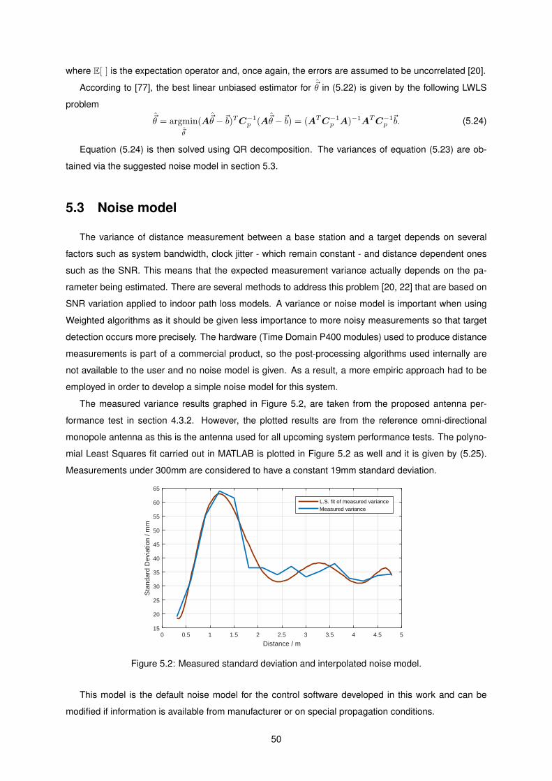
53 Noise model 50
54 Real-Time Tracking and path smoothing 51
55 The Tracking Algorithm 54
56 Performance Analysis 54
561 Static target 55
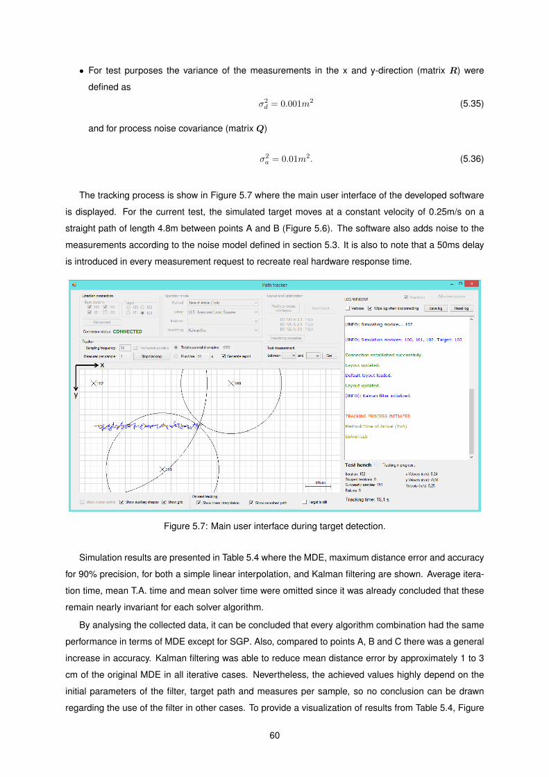
562 Target moving on a straight path 59
57 Summary 61
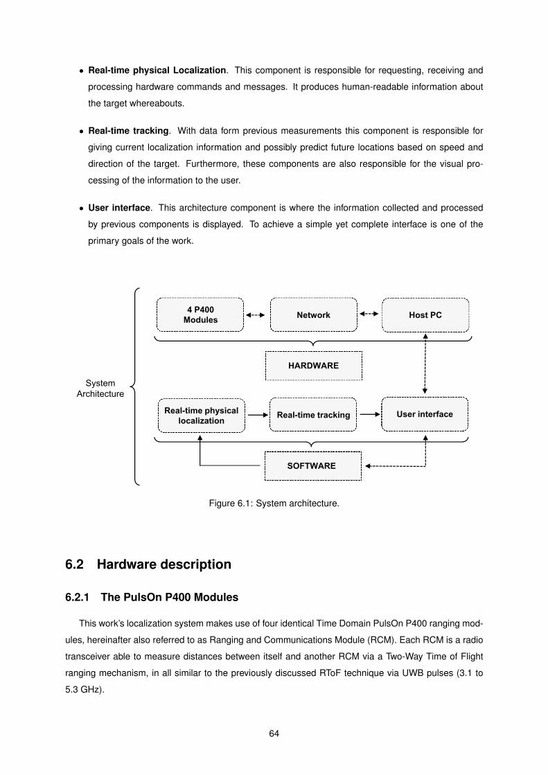
6 System architecture 63
61 Introduction 63
62 Hardware description 64
621 The PulsOn P400 Modules 64
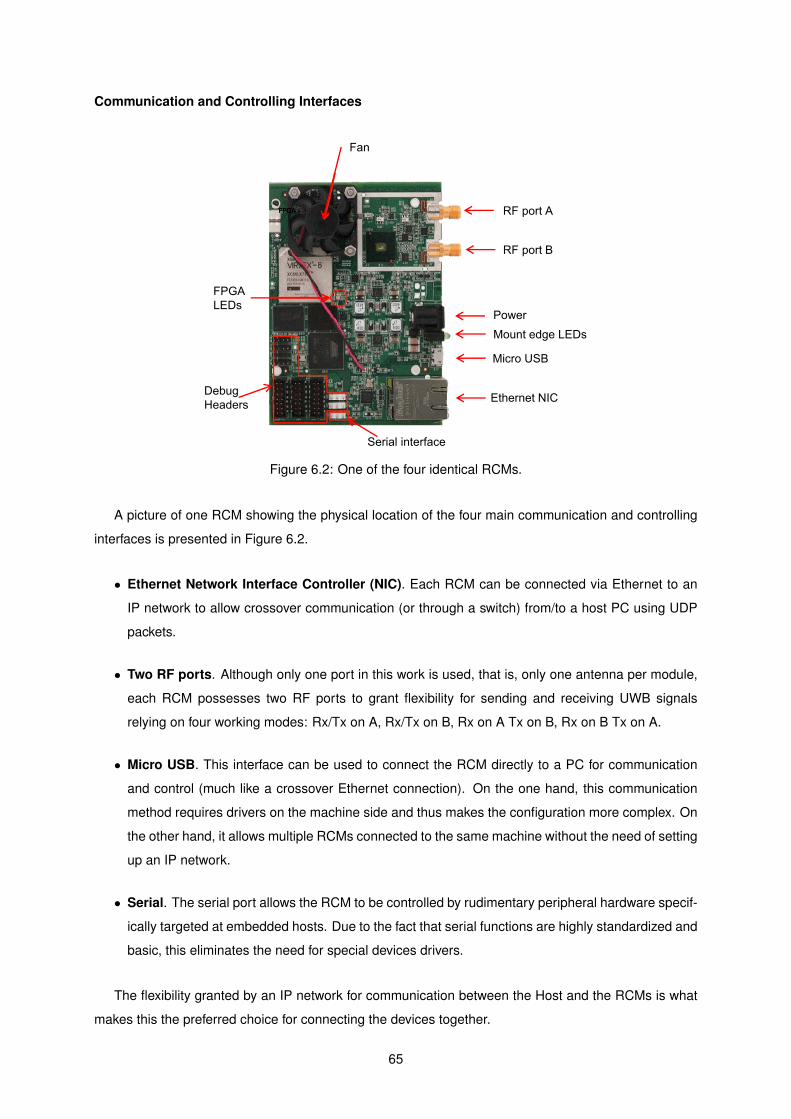
Communication and Controlling Interfaces 65
Round-trip Time of Flight Ranging 66
622 Network environment and communication 66
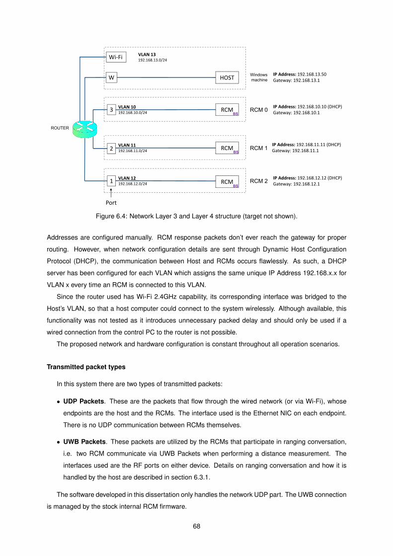
Network Layout 66
Transmitted packet types 68
63 Software description 70
631 Application structure 71
xii
Tracker class 71
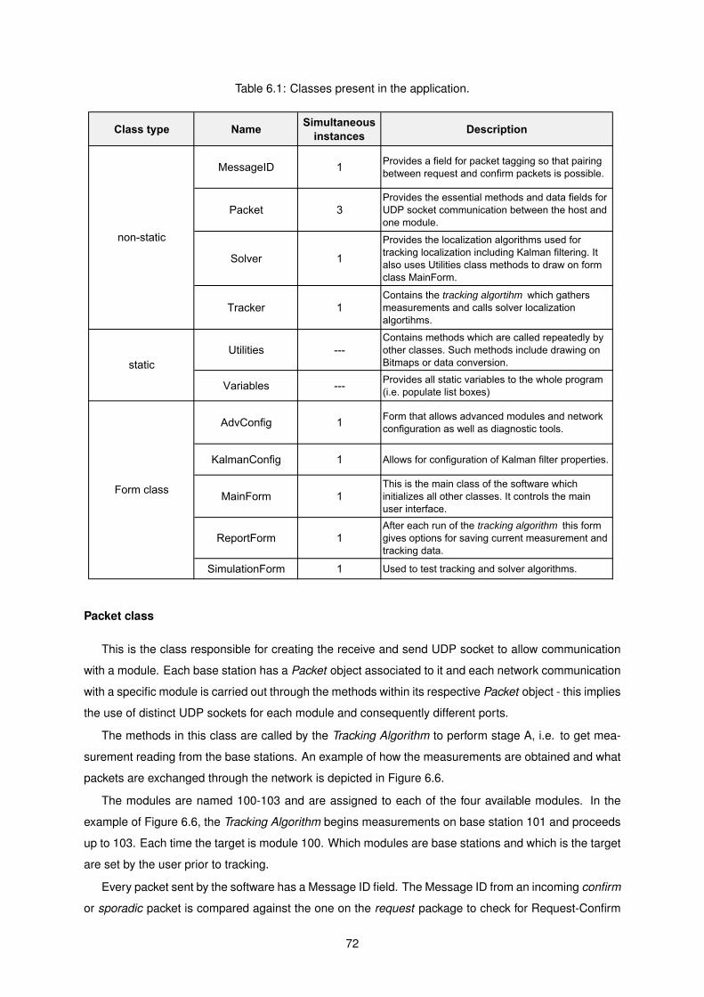
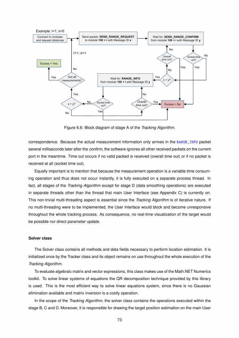
Packet class 72
Solver class 73
64 Summary 74
7 Conclusion and future work 77
71 Future Work 78
References 81
A Connector model 87
B Radiation patterns of UWB antenna 89
C Software User Interface 91
C1 Main User Interface 91
C2 Advanced Options 92
C3 New base station layout 93
C4 Smoothing options 93
C5 Simulation console 93
C6 Tracking report 94
D Example of layout input file 97
xiii
xiv
List of Tables
21 Overview of presented technologies 17
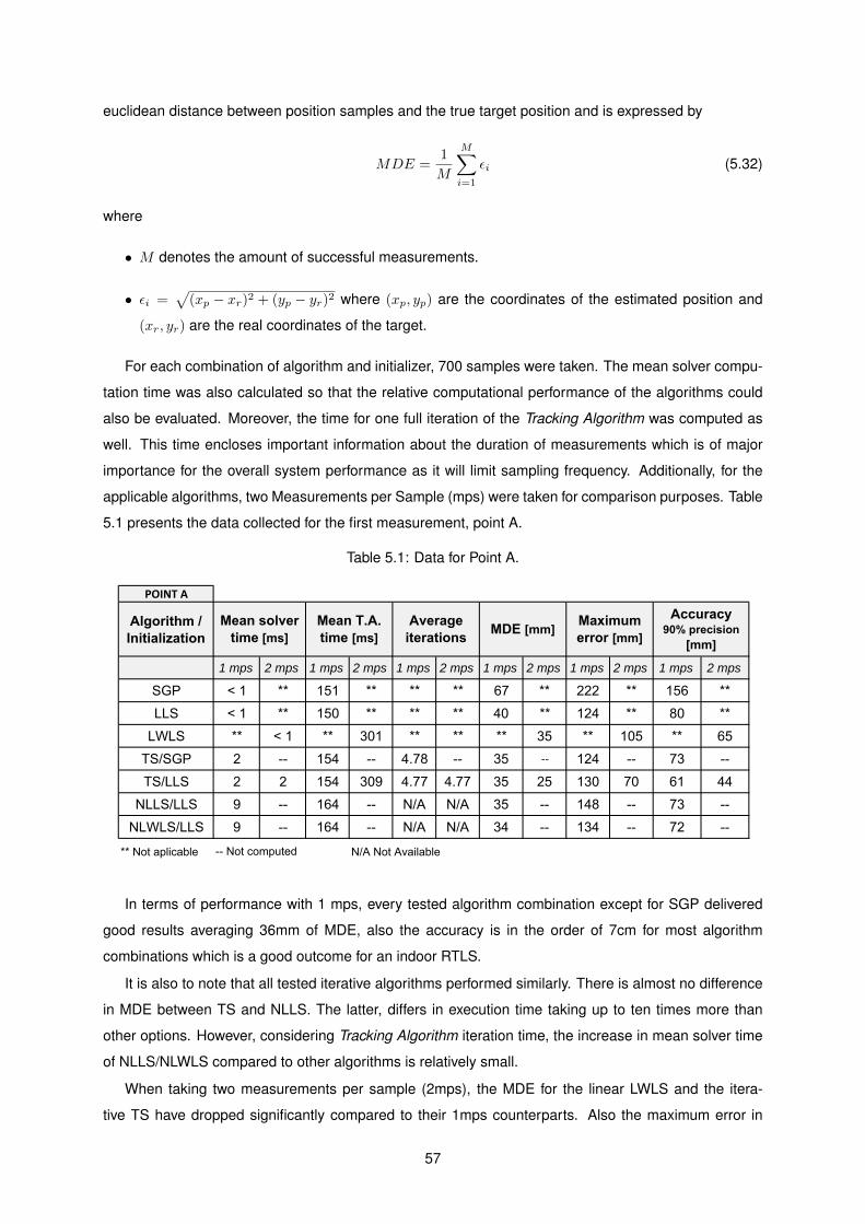
51 Data for Point A 57
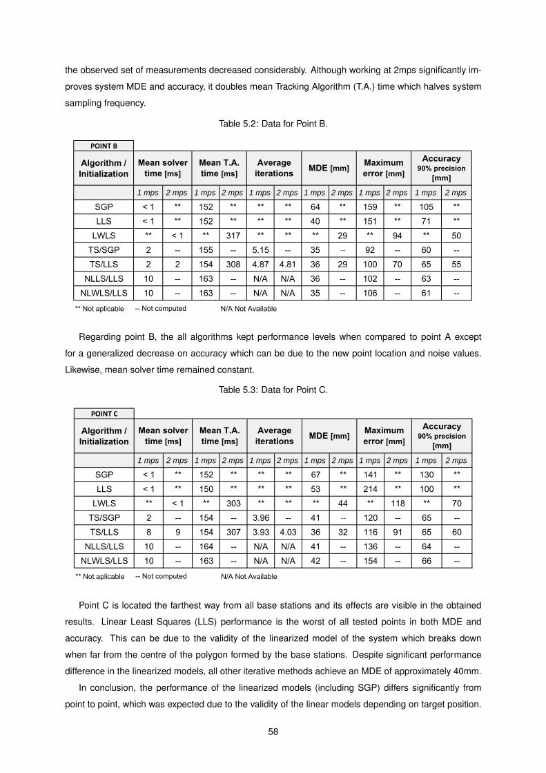
52 Data for Point B 58
53 Data for Point C 58
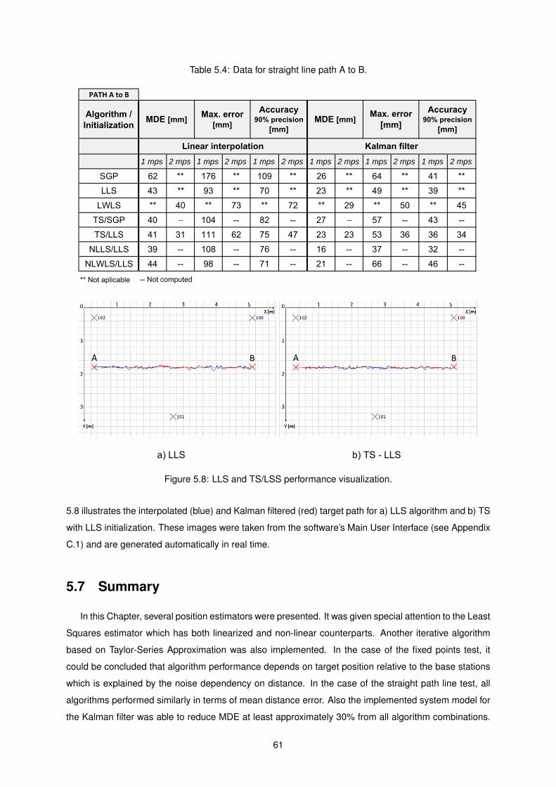
54 Data for straight line path A to B 61
61 Classes present in the application 72
C1 Fields of tracking log file 95
xv
xvi
List of Figures
11 Illustration of a simple localization system 2
21 Illustration of network operating modes 7
22 Fingerprinting Unknown nodersquos location P is estimated according to off-line RSSI mea-
surements 8
23 Positioning based on RSSI and ToA measurements 11
24 Positioning using the time difference of arrival of an RF and an ultrasound signal 11
25 TDoA positioning (only the relevant branch of the hyperbola is shown for each measure-
ment) 12
26 AoA positioning 14
27 Examples of devices used in two presented location systems 16
31 Antenna types for indoor location 21
32 Examples of Inverted F and Meander antennas 23
33 Meander antenna for RFID Tag 23
34 Microstrip rectangular and circular patch Antenna excitation from underneath via probe
feed 24
35 Illustration of received power in a multipath environment 25
36 Typical UWB monopoles design 27
37 Illustration of two UWB circularly polarized antennas 28
38 Depiction of the dielectric loading sandwich technique 28
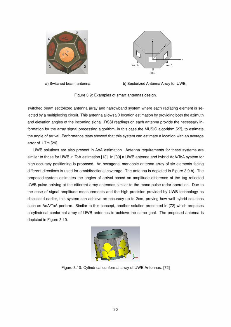
39 Examples of smart antennas design 30
310 Cylindrical conformal array of UWB Antennas 30
41 Stock UWB monopole variation 32
42 Base model for the proposed UWB antenna design - reflector plane and SMA connector
not shown (dimentions in mm) 33
43 Perspective and side view of the antenna model with reflector plane and SMA connector
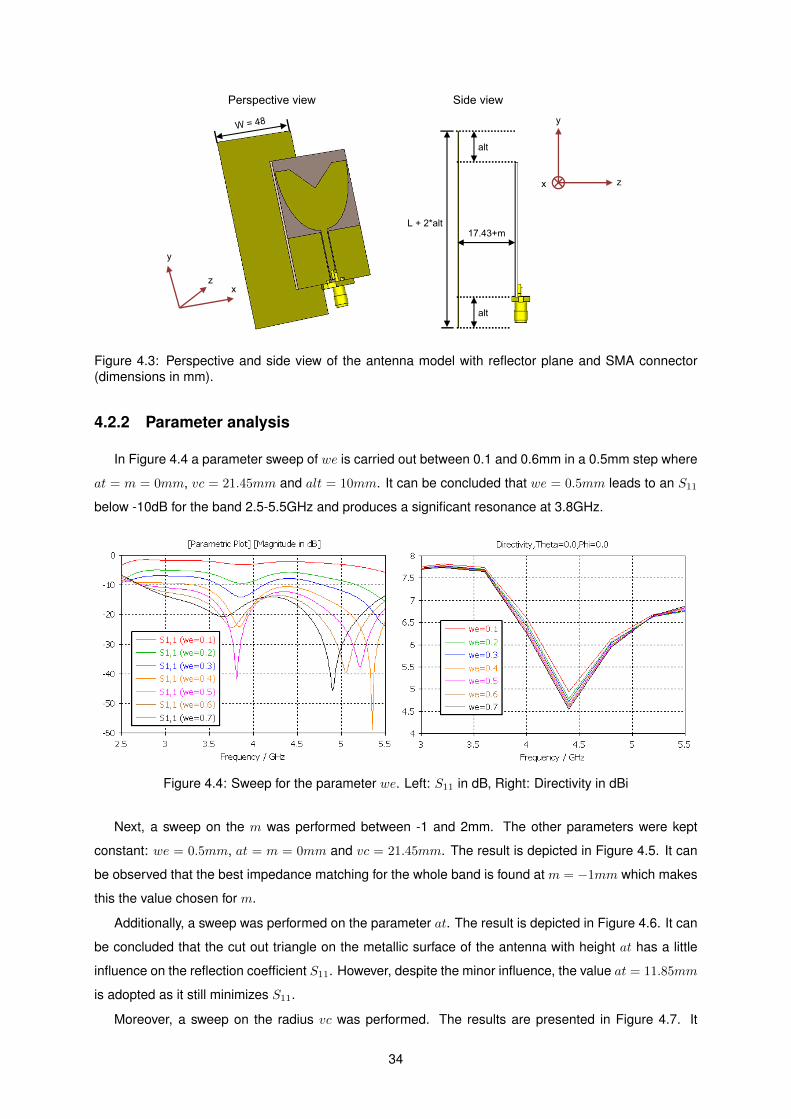
(dimensions in mm) 34
44 Sweep for the parameter we Left S11 in dB Right Directivity in dBi 34
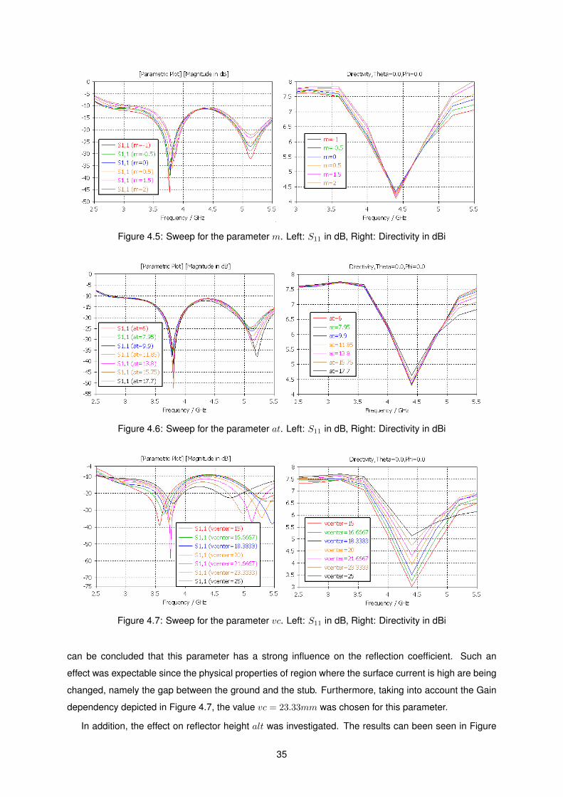
45 Sweep for the parameter m Left S11 in dB Right Directivity in dBi 35
46 Sweep for the parameter at Left S11 in dB Right Directivity in dBi 35
xvii
47 Sweep for the parameter vc Left S11 in dB Right Directivity in dBi 35
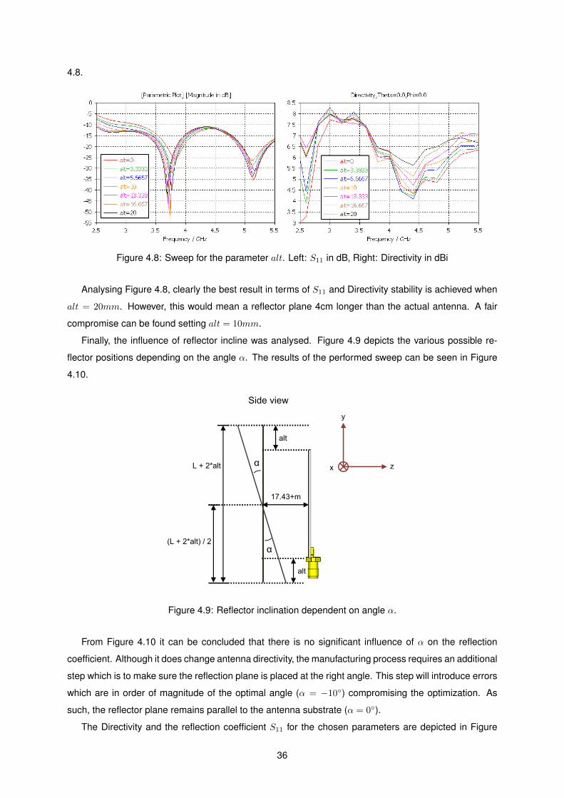
48 Sweep for the parameter alt Left S11 in dB Right Directivity in dBi 36
49 Reflector inclination dependent on angle α 36
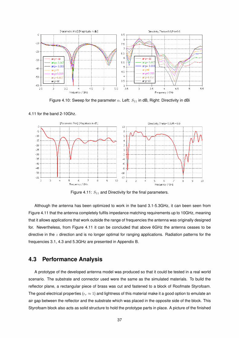
410 Sweep for the parameter α Left S11 in dB Right Directivity in dBi 37
411 S11 and Directivity for the final parameters 37
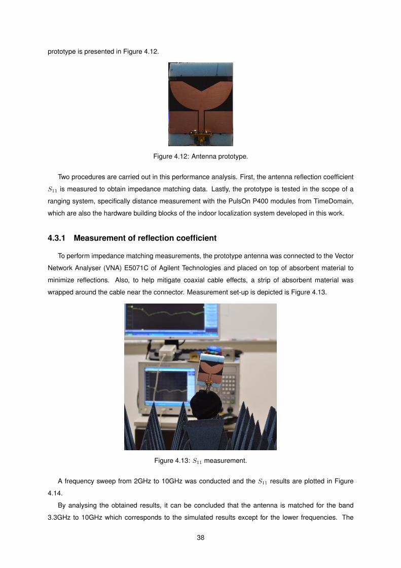
412 Antenna prototype 38
413 S11 measurement 38
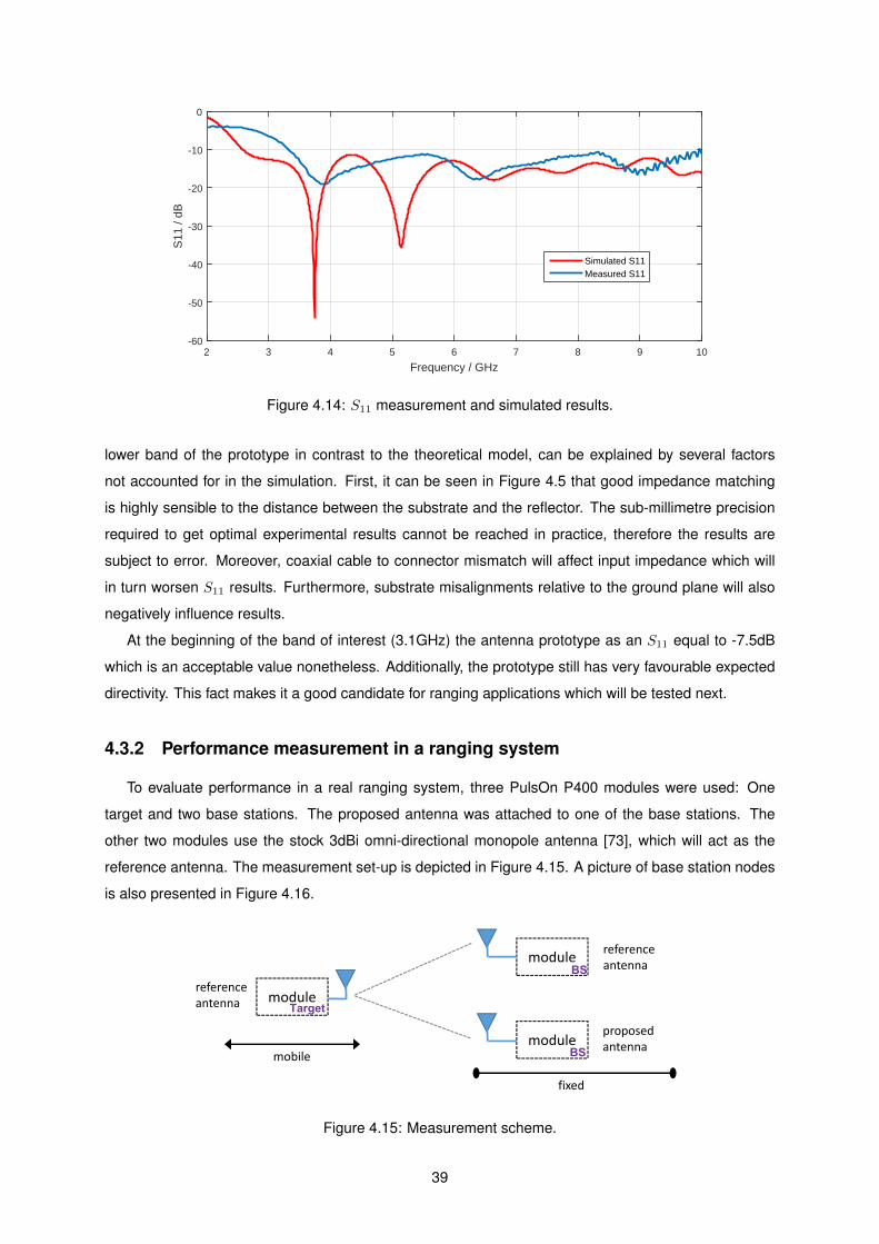
414 S11 measurement and simulated results 39
415 Measurement scheme 39
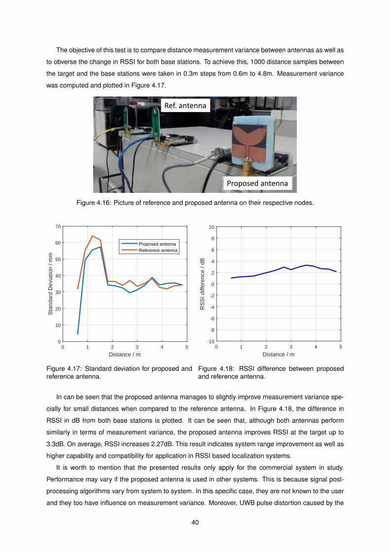
416 Picture of reference and proposed antenna on their respective nodes 40
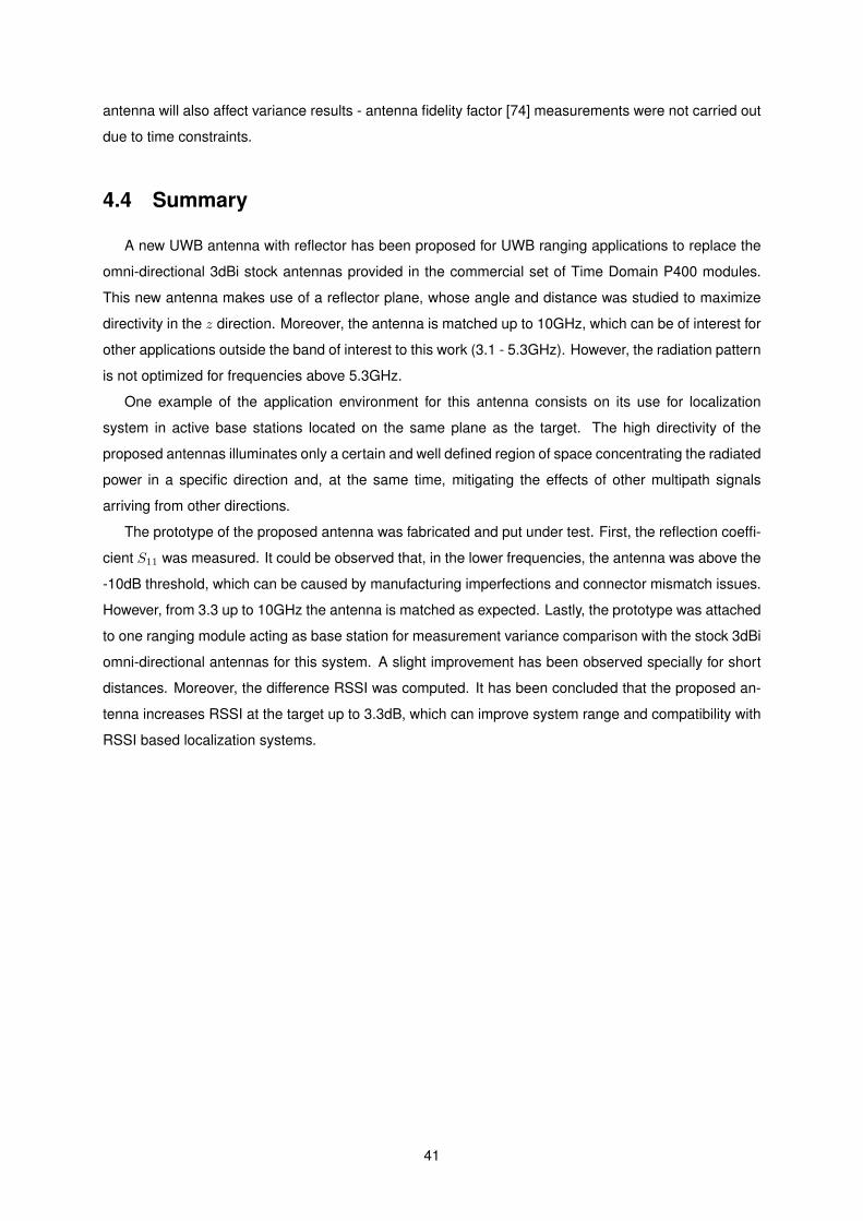
417 Standard deviation for proposed and reference antenna 40
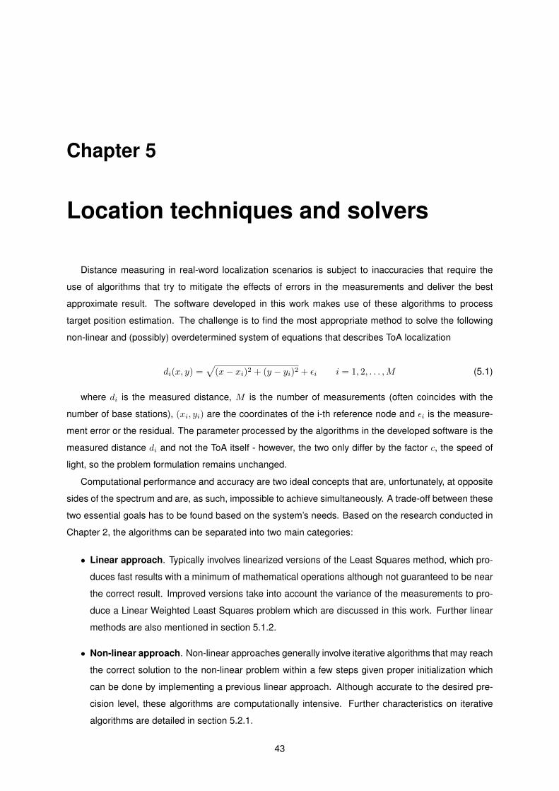
418 RSSI difference between proposed and reference antenna 40
51 Cluster of ToA estimation 44
52 Measured standard deviation and interpolated noise model 50
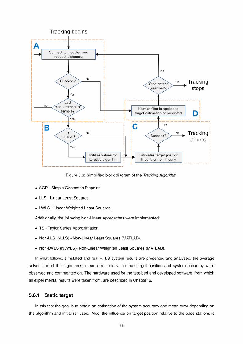
53 Simplified block diagram of the Tracking Algorithm 55
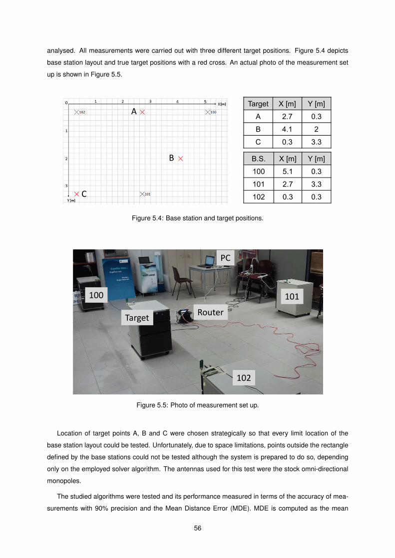
54 Base station and target positions 56
55 Photo of measurement set up 56
56 Straight line path to be tested 59
57 Main user interface during target detection 60
58 LLS and TSLSS performance visualization 61
61 System architecture 64
62 One of the four identical RCMs 65
63 Network of RCMs 67
64 Network Layer 3 and Layer 4 structure (target not shown) 68
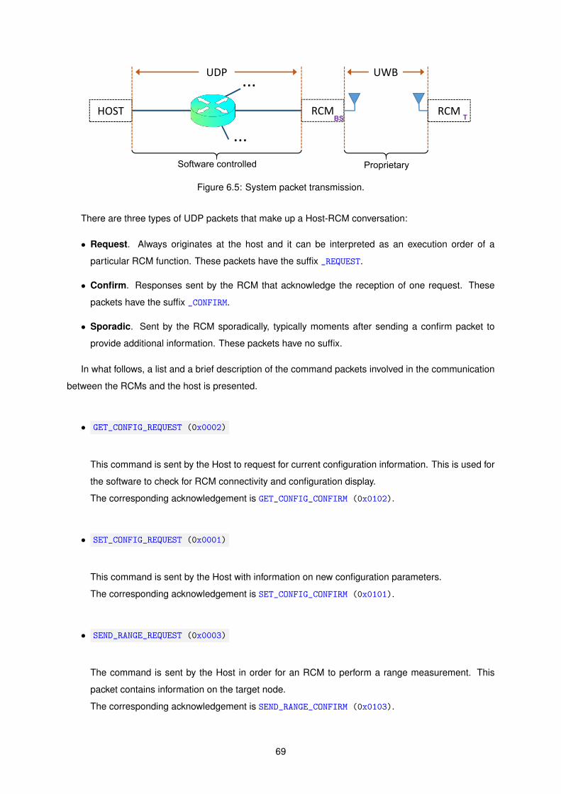
65 System packet transmission 69
66 Block diagram of stage A of the Tracking Algorithm 73
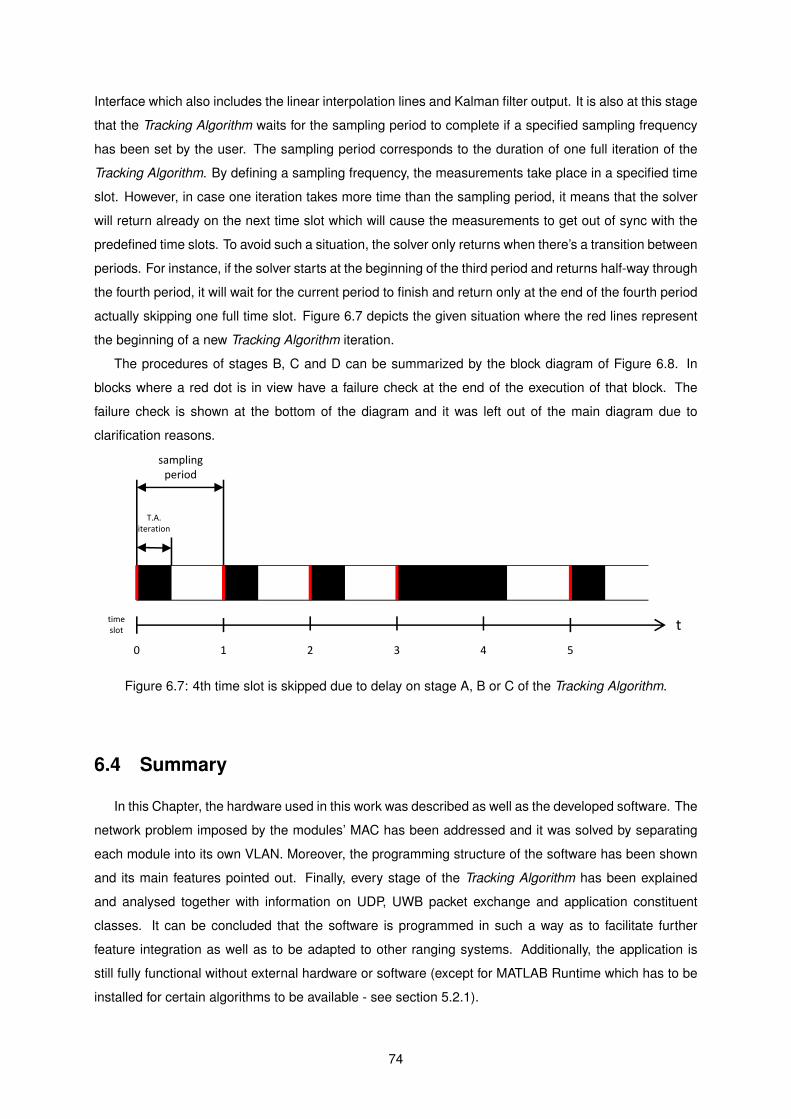
67 4th time slot is skipped due to delay on stage A B or C of the Tracking Algorithm 74
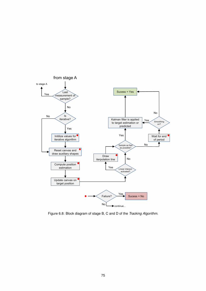
68 Block diagram of stage B C and D of the Tracking Algorithm 75
A1 SMA connector 87
A2 CST model of SMA connector 87
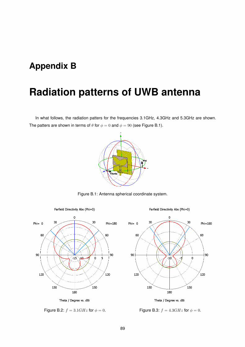
B1 Antenna spherical coordinate system 89
B2 f = 31GHz for φ = 0 89
B3 f = 43GHz for φ = 0 89
B4 f = 53GHz for φ = 0 90
B5 f = 31GHz for φ = 90 90
B6 f = 43GHz for φ = 90 90
B7 f = 53GHz for φ = 90 90
xviii
C1 Main User Interface 91
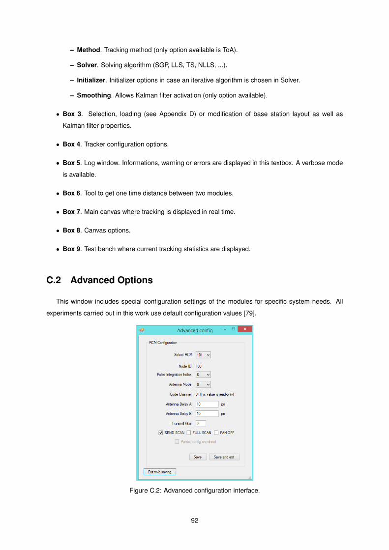
C2 Advanced configuration interface 92
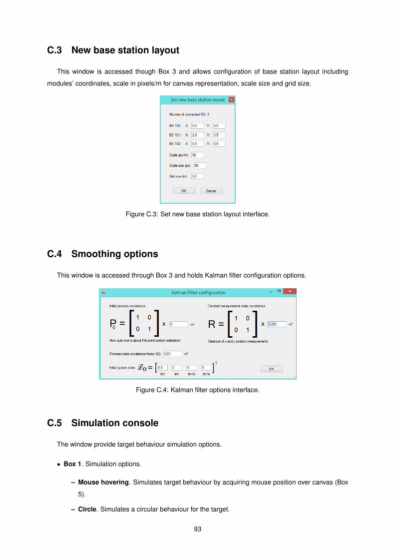
C3 Set new base station layout interface 93
C4 Kalman filter options interface 93
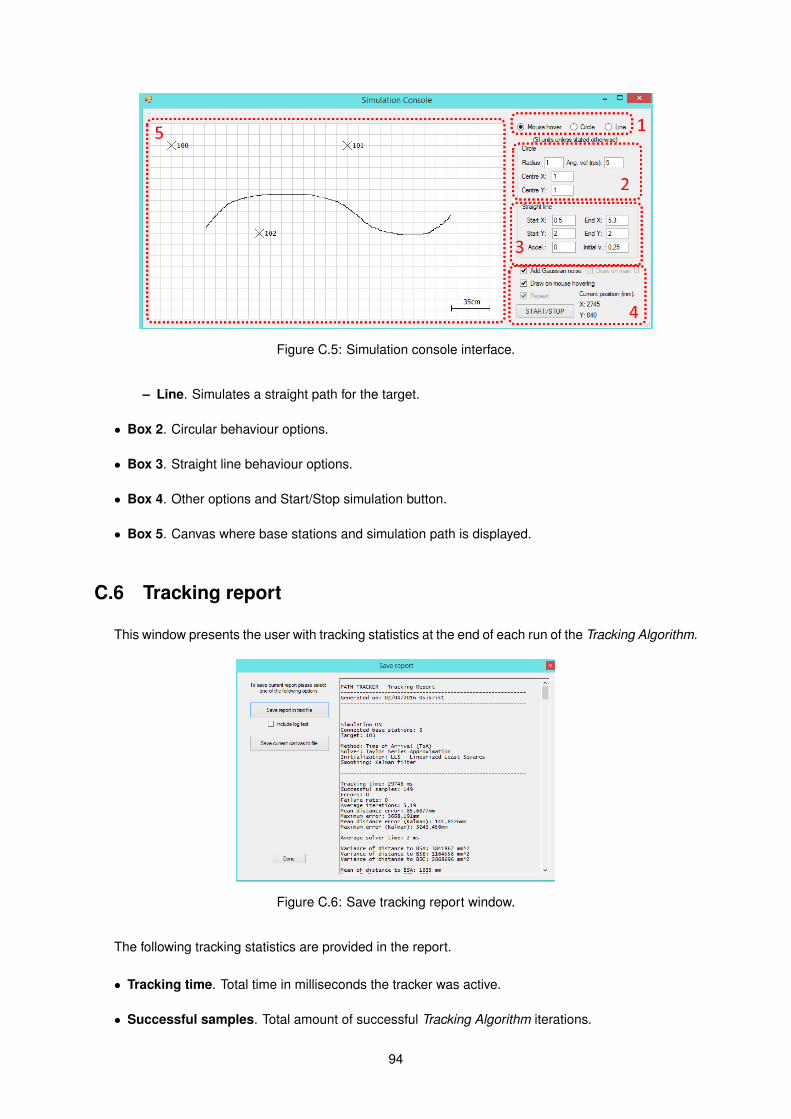
C5 Simulation console interface 94
C6 Save tracking report window 94
xix
xx
List of Acronyms
AoA Angle of Arrival
AP Access Point
API Application Programming Interface
BIA Burned-In Address
BS Base Station
CDMA Code-Division Multiple Access
Cell-ID Cell Identification
CLWLS Constrained Linear Weighted Least Squares
CPW Coplanar Waveguide
CRLB Cramer-Rao Lower Bound
DHCP Dynamic Host Configuration Protocol
DoA Direction of Arrival
DSSS Direct Sequence Spread Spectrum
GNSS Global Navigation Satellite System
GPS Global Positioning System
GUI Graphical User Interface
LLS Linear Least Squares
LoS Line of Sight
LS Least Squares
LWLS Linear Weighted Least Squares
MAC Media Access Control
MDE Mean Distance Error
ML Maximum Likelihood
mps Measurements per Sample
MSE Mean Squared Error
NIC Network Interface Controller
NLLS Non-Linear Least Squares
NLoS Non Line of Sight
NLWLS Non-Linear Weighted Least Squares
OSI Open Systems Interconnection
xxi
PCB Printed Circuit Board
PIFA Planar Inverted-F Antenna
RCM Ranging and Communications Module
RF Radio Frequency
RFID Radio Frequency Identification
RSSI Received Signal Strength Indicator
RTLS Real-Time Localization System
RToF Round-trip Time of Flight
SAA Sectorized Antenna Array
SGP Simple Geometric Pinpoint
SNR Signal-to-Noise ratio
TA Tracking Algorithm
TDoA Time Difference of Arrival
ToA Time of Arrival
TS Taylor Series Approximation
UDP User Datagram Protocol
UHF Ultra-High Frequency
UWB Ultra Wide Band
VLAN Virtual Local Area Network
VNA Vector Network Analyser
Wi-Fi Wireless Fidelity
xxii
Chapter 1
Introduction
11 Motivation and objectives
Since the inception of wireless propagation but specially in the last 10 to 15 years there has been
a non-stop development in the area of location techniques The capacity growth of devices that help
locate someone or something on a given site has been tremendous More and more the utilities and
capabilities of wireless propagation techniques have become increasingly relevant in this scientific field
Antennas are one of the most important components in a localization system They are the entrance
and exit points for information when itrsquos transmitted wirelessly Improvements in the area are almost
limitless and there is still a lot of research to be done Today with modern simulation techniques one
can almost develop a full working model on the computer by means of advanced simulation software
However the testing phase cannot be left aside The usefulness of the fine tuning ensuing the testing
phase is indubitably as relevant The potential of these methods and their ability to adapt to new scientific
challenges is one of the reasons why this subject is so interesting and promising
Alongside the development of a localization system therersquos the need for developing software that
analyses processes and presents the user with human readable and useful information The variety of
possibilities in regards to programming language platforms and environments allow for a very versatile
and complete solution
The purpose of localization systems is vast and concerns many scientific fields and services such
as medical and healthcare monitoring inventory location global positioning or even personal tracking
These fields have developed a need for the so-called Location Awareness The constant improvement of
such systems is imperative as they must keep up with constant new challenges and necessities Overall
the goal is to reduce complexity increase resilience and maintain operation capacity throughout usage
time despite external factors such as interference user interaction or physical damage
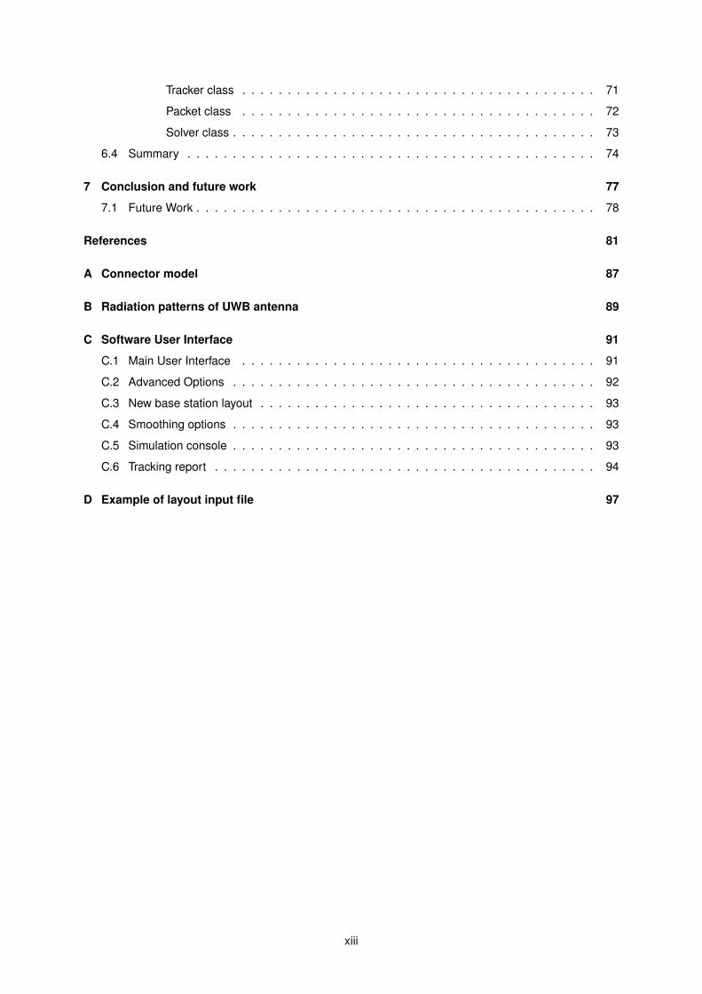
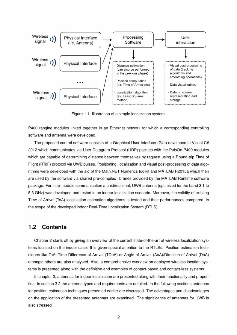
Figure 11 illustrates de concept of a complete localization network or system and its central func-
tions First the network wireless signals enter the physical interface They are then processed according
to the systemrsquos needs and finally presented to the user The objective of this work is to provide a fully
functional Ultra Wide Band (UWB) indoor localization system making use of four Time Domain PulsOn
1
Physical Interface(ie Antenna)
Wireless signal
Physical Interface
Physical Interface
Processing Software
Wireless signal
Wireless signal
Userinteraction
- Distance estimation (can also be performed in the previous phase)
- Position computation (ex Time of Arrival etc)
- Localization algorithm (ex Least Squares method)
- Visual post-processing of data (tracking algorithms and smoothing operations)
- Data visualization
- Data on screen representation and storage
Figure 11 Illustration of a simple localization system
P400 ranging modules linked together in an Ethernet network for which a corresponding controlling
software and antenna were developed
The proposed control software consists of a Graphical User Interface (GUI) developed in Visual C
2012 which communicates via User Datagram Protocol (UDP) packets with the PulsOn P400 modules
which are capable of determining distance between themselves by request using a Round-trip Time of
Flight (RToF) protocol via UWB pulses Positioning localization and visual post-processing of data algo-
rithms were developed with the aid of the MathNET Numerics toolkit and MATLAB R2015a which then
are used by the software via shared pre-compiled libraries provided by the MATLAB Runtime software
package For intra-module communication a unidirectional UWB antenna (optimized for the band 31 to
53 GHz) was developed and tested in an indoor localization scenario Moreover the validity of existing
Time of Arrival (ToA) localization estimation algorithms is tested and their performances compared in
the scope of the developed indoor Real-Time Localization System (RTLS)
12 Contents
Chapter 2 starts off by giving an overview of the current state-of-the-art of wireless localization sys-
tems focused on the indoor case It is given special attention to the RTLSs Position estimation tech-
niques like ToA Time Difference of Arrival (TDoA) or Angle of Arrival (AoA)Direction of Arrival (DoA)
amongst others are also analysed Also a comprehensive overview on deployed wireless location sys-
tems is presented along with the definition and examples of contact-based and contact-less systems
In chapter 3 antennas for indoor localization are presented along with their functionality and proper-
ties In section 32 the antenna types and requirements are detailed In the following sections antennas
for position estimation techniques presented earlier are discussed The advantages and disadvantages
on the application of the presented antennas are examined The significance of antennas for UWB is
also stressed
2
In chapter 4 an UWB antenna for ranging communication is proposed The idea behind a new design
lies on the use of a metallic reflector plane which concentrates power on a given direction Optimization
details and performance are also evaluated
In chapter 5 the localization and tracking algorithms used by this system are introduced Various
proposals are made to be used in the RTLS In addition by using the developed control software the
algorithms are tested and its performance commented on
In chapter 6 the system architecture is presented Not only the hardware and network parts are
explained but also the software development and its usefulness are demonstrated
In chapter 7 the final conclusions about the work are drawn Also future work topics are suggested
3
4
Chapter 2
Outline of localization systems
In this chapter the definition and application of a general localization system as well as an overview
of the underlying localization estimation techniques are introduced The concept of a Real Time Local-
ization System is also presented Furthermore the current knowledge in this field recent developments
that have occurred and some already developed location systems are exposed
21 Introduction
A location or localization system is a set of operational devices which possess specific hardware
and software to compute and locate the position of a moving or stationary object in a given site These
systems are made of nodes that can represent devices to be located (unknown nodes dark nodes or
target nodes) or reference points whose location is known (reference nodes or base stations) The goal
of such systems is to provide a more-or-less precise and accurate location of the object depending on
its characteristics and function A system that does this in real-time is called an RTLS One application
of the RTLSs is the already mentioned medical services for example More in-depth location estimation
within hospitals or outdoor ambulance tracking helps the medical emergency service to function more
efficiently Another application of RTLS is the very classic navigation An RTLS such as the Global
Positioning System (GPS) [1] can be used to simply find directions or in a more complex scenario to
aid traffic management
Moreover tracking services also employ RTLSs These can include people vehicle personnel or
product tracking [2] As an example a study presented in [3] reveals that through user localization in
indoor construction environments immediate and opportune access to project relevant information can
be useful for time efficiency and cost reduction Other social services where mostly outdoor RTLS can
be implemented include information marketing and billing [2]
A location system can be differentiated by specific characteristics or properties As expected despite
the physical properties of the system and its applications the required estimation accuracy and preci-
sion varies significantly depending on the goal the system is trying to achieve and the hardware used
Moreover the working environment whether it is indoor or outdoor is also an important characteristic
5
Similarly the system can be either contact of contact-less based Finally the used location techniques
are also an important aspect
In what follows the mentioned characteristics will be analysed in detail Along with the analysis
examples of currently deployed systems will be presented and referenced in the scope of each property
A special emphasis will be given to the location techniques since itrsquos one of the main subjects of this
dissertation
22 Technical aspects of location systems
In this section several technical aspects are presented These include the concept of operation
mode accuracy and precision as well as basic location techniques
The estimation of localization can be divided into three categories or steps Distanceangle estima-
tion position computation and visual post-processing Information gathered by the sensors or devices
will travel these 3 steps in order In section 223 it will be given special attention to distanceangle es-
timation which is the component responsible for computing the distance or angle between two nodes
In the same section position computation techniques like Fingerprinting Tri- and Multilateration will be
introduced Additionally some position estimation algorithms which will compute the nodes location
with respect to existing reference nodes or points will be mentioned Visual processing is part of the
developed software which will be briefly mentioned in posterior Chapters
221 Network topology
Location systems are based on an underlying network regardless of the technology used According
to [4] one can distinguish between three major types of fundamental topologies or operation modes
Infrastruture mode The devices used in such an operation mode are part of an infrastructure of
previously placed reference nodes which the devices are connected to There is no direct communication
between devices This allows for a flexible connectiondisconnection of nodes to or from the network
because they do not depend on each other However this added complexity requires more equipment
and configuration necessities In Wireless Fidelity (Wi-Fi) networks for example the reference nodes
are Access Points (AP) to which Wi-Fi enabled devices connect to An example of network operating in
an infrastructure mode is presented in Figure 21 a)
Ad-hoc mode In this operation topology the devices or sensors do not depend on a previously
existing network to communicate or on any central administration The communication is done in a peer-
to-peer fashion Because each device acts as its own router network management and fault detection
is a difficult task to accomplish [5] The ZigBee standard [6] supports this operation mode and is an
example of recent application Figure 21 b) depicts an ad-hoc network composed of mobile devices
Deduced or dead reckoning This is an operation mode where the system estimates an objectrsquos
current position by inferring it from the last previous known location together with speed and trajectory
information The device estimates its own location by itself without external communication Inertial
6
AP1
AP3
AP2
AP3Switch
a) Infrastructure mode b) Ad-hoc mode
Figure 21 Illustration of network operating modes
Navigation [7] is a currently used form of dead reckoning
222 Accuracy and precision
The rigour of a location estimation system is a characteristic of great importance In the literature by
introducing the concept of Accuracy and Precision it can be classified how well the location estimation
system behaves [8]
Accuracy or granularity denotes how close an estimation is to the real value In the case of location
systems a higher accuracy (finer granularity) means a lower spatial error margin relative to the true
location It is expressed in units of length and it usually arises in the form of a range of values Preci-
sion denotes how likely it is for the estimated value to lie within a certain accuracy interval or above a
threshold
Accuracy of location systems vary within orders of magnitude It typically ranges from centimetres up
to kilometres depending on propagation environment (indoor or outdoor) as well as on their application
goal and available technology Table 21 summarizes the expected accuracy and precision for some of
the briefly presented location systems in section 232
223 Location techniques
In what follows special attention will be given to basic techniques for location determination in which
methods like Received Signal Strength Indicator (RSSI) ToA TDoA AoADoA and RToF are included
Along with the analysis the most used estimation algorithms are briefly mentioned
Received Signal Strength Indicator (RSSI)
The RSSI can be used to estimate a distance between two nodes using only the measured signal
strength (or a value proportional to it) received from one of the nodes A common model to relate the
average received power with the distance travelled by the signal is given by [9]
P (d) = P0 minus 10ntimes log10(dd0) (21)
7
where P0 is the power in dB received at the reference distance d0 and n is called the path loss exponent
Despite this modelrsquos simplicity the instantaneous power received is subject to multipath effects such
as reflection scattering and diffraction which foment a rapid received power variation over short time
intervals or distances This effect can be mitigated by computing the mean of the power received over
a certain period of time T However there can be no Line of Sight (LoS) and so the signal suffers
from shadowing and a slower power variation still occurs around its mean [9] Signal power variation
in linear units caused by this fading can be modelled by a log-normal distribution with a certain mean
and variance σ2 Propagation conditions depend on a constant scenario variation when the node to be
located constantly moves This makes it difficult to properly define an accurate path loss exponent n and
variance σ2 The type of antenna and node orientation must also be taken into account These effects
corrupt the measured quantity therefore the distance estimation is mostly inaccurate using solely this
method
Most available receivers are able to measure the RSSI without any special additional hardware [10]
This means that systems based in RSSI can have a reduced cost This brings a problem however
although a RSSI based location can be a inexpensive solution low-cost modules commonly possess
poorly calibrated components This not only affects RSSI readings but also the transmitted power As
an example an experiment in [11] obtained estimation accuracies in the order of a few metres using
WINS Sensor nodes [12] placed at ground level The same experiment shows that RSSI can be very
unpredictable and highly dependable on distance between reference nodes
xP
A
B
C
1 2 3 4
5 6 7 8
A B C
1 RSSI RSSI RSSI
2 RSSI RSSI RSSI
3 RSSI RSSI RSSI
hellip hellip hellip hellip
Off‐line calibration point
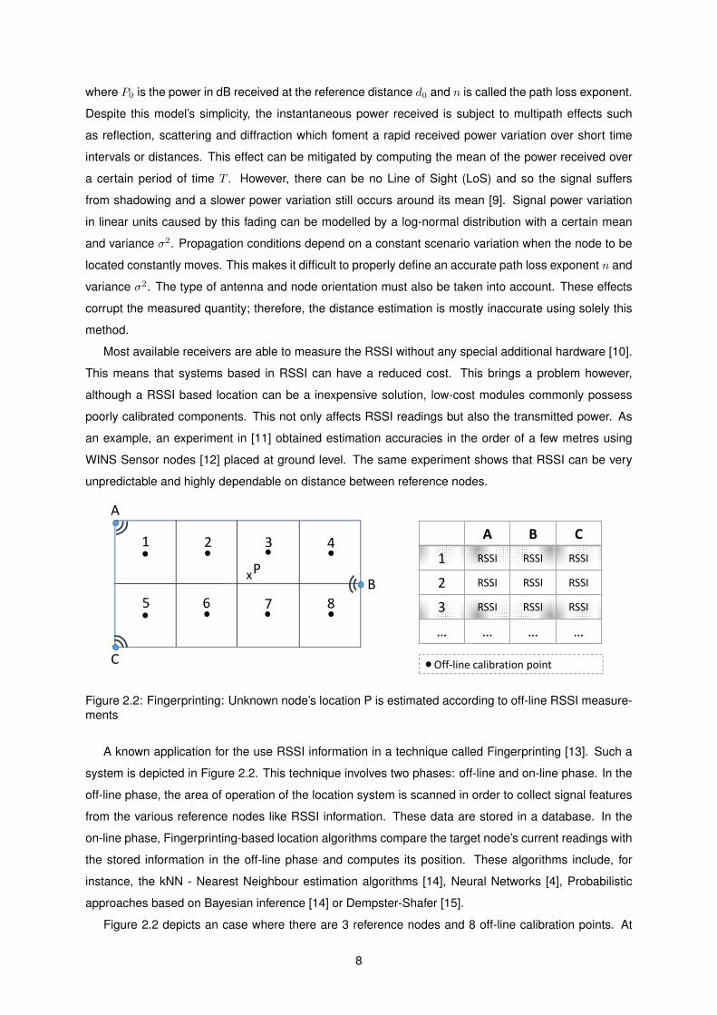
Figure 22 Fingerprinting Unknown nodersquos location P is estimated according to off-line RSSI measure-ments
A known application for the use RSSI information in a technique called Fingerprinting [13] Such a
system is depicted in Figure 22 This technique involves two phases off-line and on-line phase In the
off-line phase the area of operation of the location system is scanned in order to collect signal features
from the various reference nodes like RSSI information These data are stored in a database In the
on-line phase Fingerprinting-based location algorithms compare the target nodersquos current readings with
the stored information in the off-line phase and computes its position These algorithms include for
instance the kNN - Nearest Neighbour estimation algorithms [14] Neural Networks [4] Probabilistic
approaches based on Bayesian inference [14] or Dempster-Shafer [15]
Figure 22 depicts an case where there are 3 reference nodes and 8 off-line calibration points At
8
each point RSSI information from reference nodes A to C has been gathered and stored in the table
The main advantage of Fingerprinting is that RSSI reading errors caused by the application environment
have already been taken into account in the off-line phase It is this a priori calibration that makes this
technique suitable for indoor environments Nevertheless the need for a central system for database
storage off-line calibration which needs to be updated in case of environment changes and algorithms
complexity render the solution complex and time-consuming
Time of Arrival (ToA)
The distance between two nodes can also be measured in terms of the time it takes for the signal
to travel between them Supposing v is the propagation speed of the signal then d = v times (t2 minus t1)
where d is the distance between the nodes and t1 and t2 are the times at which the signal was sent and
received respectively This technique can provide highly accurate results [10] However the calculation
of d requires the times t1 and t2 to be measured by different nodes in the network This implies time
stamp information transfer between devices as well as prior clock synchronization of the network These
aspects will rise hardware complexity and system cost
Assuming that all transmitters emit a pure sinusoidal wave the ToA can be measured by identifying
the phase of arrival of the carrier signal Some type of synchronism must be present for example emis-
sion with a known phase offset Nevertheless this method is highly susceptible to multipath fading which
is a common occurrence in indoor environments For this reason narrowband signals are inadequate
to be used in this method More complex techniques like Direct Sequence Spread Spectrum (DSSS) or
UWB contribute to reduce the effects of multipath due to their short duration in the time domain There-
fore these signals are more suitable for a ToA based location estimation [16 17] The use of UWB for
ToA applications is analysed in detail in section 34
Conventional ToA estimation involves the use of correlators or matched filter receivers [9] The
former correlates the received signal with a template signal for various time delays The time delay that
produces the correlation peak is the estimated ToA The latter works by using a filter matched to the
transmitted signal which outputs its largest value at the instant of signal reception Both methods are
subject to errors due to electromagnetic and hardware noise In the absence of LoS first-path detection
algorithms like in [18] or [19] must be applied in order to detect the first arriving signal rather than
possibly stronger multipath originating copies which would impose false correlator and filter outputs [9]
ToA measurements merely infer the time it takes for a signal to arrive at a node so that a distance
can be computed However the direction of signal arrival is still unknown Trilateration is a technique
for locating an unknown point based on distances to other points whose location is known Trilateration
makes use of at least three distance measurements (in 2D) to three reference nodes The distance
estimates are obtained through ToA or RSSI measurements for example In an ideal case (absence of
noise in the measured value and no multipath effects) a circumference around each reference node is
created where the target node might be located
9
The estimated distance di between the target node and the i-th reference node is given by
cti = di = fi(xi yi) + εi i = 1 2 M (22)
where ti is the actual ToA measurement c is the speed of light εi denotes the measurement error or
noise and
fi(xi yi) =radic
(xminus xi)2 + (y minus yi)2 i = 1 2 M
Equation 22 is actually a system of equations where (xi yi) are coordinates of the i-th reference
node M the number of reference nodes and (x y) the coordinates of the target node For εi = 0 when
three of these circumferences intersect a fixed location is obtained This procedure is depicted in Figure
23 a) The location is obtained by solving the system for (x y)
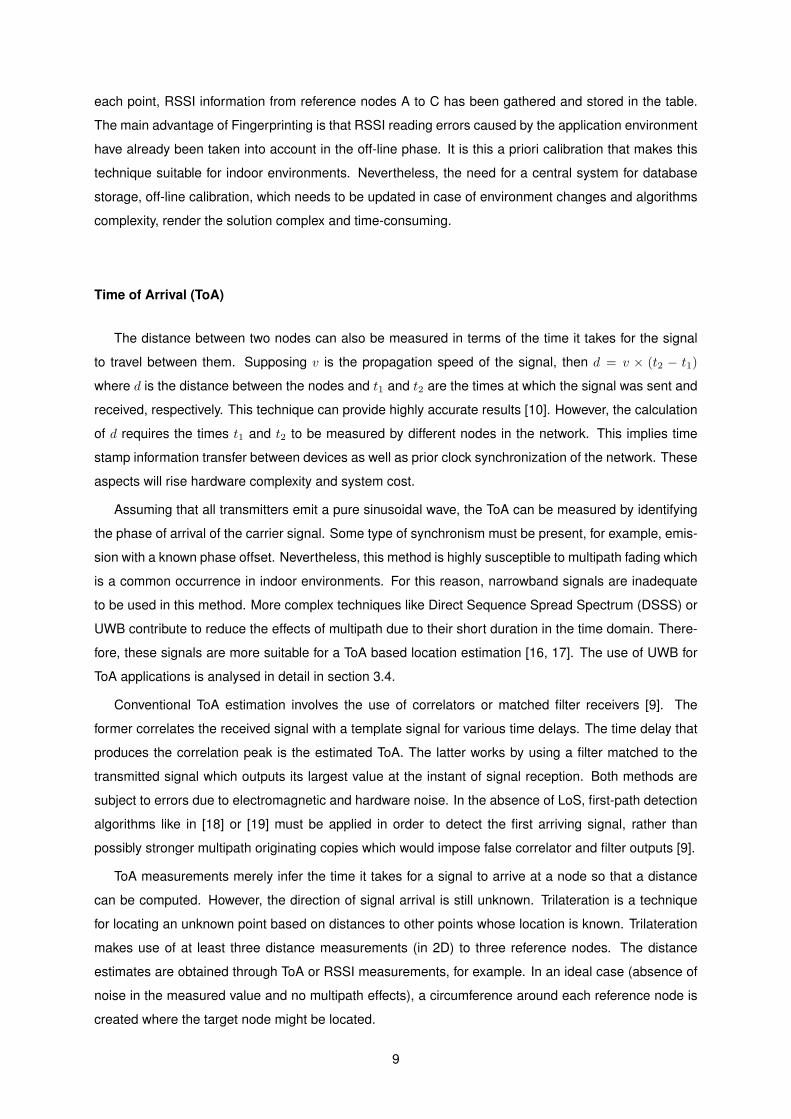
However in a real system reference node position and distance estimation inaccuracies occur
These are modelled by the noise variable εi This variable introduces the probabilistic characteristic
of this problem and so a new approach has to be applied ie the position (x y) has to be estimated
The circumferences which denote a possible position for the target node will intersect at different points
forming an area of uncertainty where the true location lies on - Figure 23 b) Moreover the system 22
is overdetermined and non-linear
To solve this statistics problem the Maximum Likelihood (ML) method can be applied [20] Under
the assumption that the noise εi is normally distributed has zero mean variance σ2i the estimator
θML = [x y]T asymptotically achieves the Cramer-Rao Lower Bound (CRLB) 1 [21] In a real system
M will be finite so in general the ML estimator will be biased and have a non-optimal variance greater
than the CRLB The final expression for θML = [x y]T corresponds to the following Non-Linear Weighted
Least Squares (NLWLS) problem [20]
θML = [x y]T = argminxy
Msumi=1
(di minus fi(x y))2
σ2i
(23)
It is noteworthy that the variance of the noises εi (ie σ2i ) are dependent on i For each of i mea-
surement there is a different variance because a different channel is used However σ2i is also distance
dependent ie the noises are heteroeskedastic [22] To improve performance a basic variance model
based on real distance measurements is developed for the location system developed in this work
The absence of a closed form solution to the NLWLS problem in (23) implies the use of iterative and
computationally intensive algorithms such as the method of Gauss-Newton or Leverberg-Marqvardt
Although providing accurate results these approaches require good parameter initialization to avoid
diverging or converging to local minima and minimize iterative steps Initialization parameters for these
algorithms can be obtained via Simple Geometric Pinpoint (SGP) or via linearization techniques The
latter can also be used to obtain an approximate closed form solution to the NLWLS problem Both SGP
and linearization are introduced and discussed in detail in Chapter 5
1The CRLB expresses a lower bound to the variance of an unbiased estimator It states that this variance is at least as high asthe inverse of the Fisher Information matrix
10
A
C
A
B
C
P
B
a) ɛ 0 b) ɛ 0
P
Figure 23 Positioning based on RSSI and ToA measurements
Time Difference of Arrival (TDoA)
This method can essentially be divided in two
bull A The difference in multiple different signal arrival times from one node at another node
bull B The difference in signal arrival times from two or more nodes at a single node
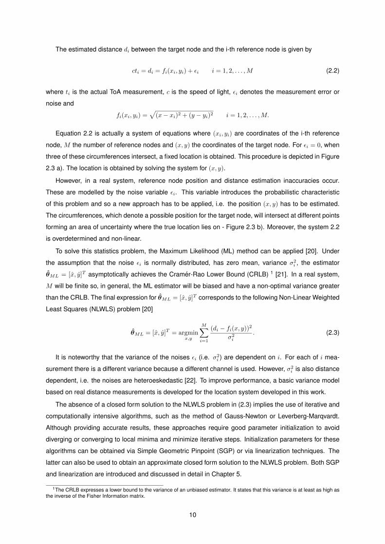
A The first method consists of sending two signals simultaneously with different and known prop-
agation speeds v1 and v2 For example a system may use Radio Frequency (RF) and ultrasound
simultaneously [23] The first one usually contains the information packet and the last one being a con-
trol signal only [9] Using basic geometry the distance between the sending and receiving node is given
by d = (v1 minus v2)(t1 minus t2) This concept is depicted in Figure 24
Transmitternode
Receivernode
Figure 24 Positioning using the time difference of arrival of an RF and an ultrasound signal
This solution does not require synchronization of the network because the distance estimate does
not depend on the absolute time the signal was sent only on the arrival difference However it requires
an additional cost in hardware due to the necessity on being able to transmit and receive two types of
signals
11
An application of this method using RFUltrasound was able to reach an accuracy of 2 centimetres
with a node distance of 3 metres [11] This solution provides high accuracy and is well suited for wireless
sensor networks [10]
B In the second type of TDoA the target node can listen to signals from nearby transmitters or
reference nodes compute their ToA and calculate the time difference of arrival for each different pair of
signalling transmitters For example with three transmitters A B and C one would have the TDoA of
A-B A-C and B-C On that note a TDoA measurement is in its essence just the composition of two
ToA measurements Considering equation (22) for ToA a TDoA measurement can be expressed as
c(ti minus tk) = di minus dk =radic
(xminus xi)2 + (y minus yi)2 minusradic
(xminus xk)2 + (y minus yk)2 + εik (24)
where i and k denote reference units and εik the error or noise in the measured distance differences
di minus dk These can be obtained by multiplying the measured time differences ti minus tk by c the speed of
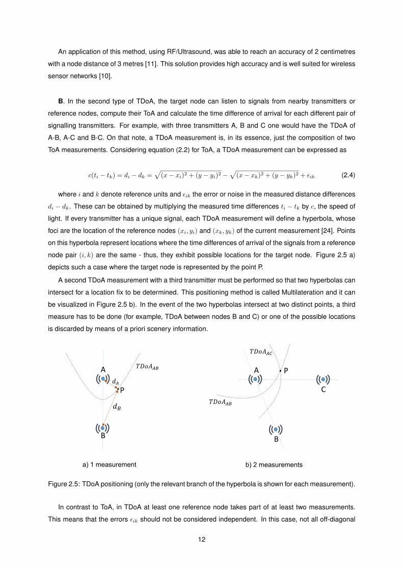
light If every transmitter has a unique signal each TDoA measurement will define a hyperbola whose
foci are the location of the reference nodes (xi yi) and (xk yk) of the current measurement [24] Points
on this hyperbola represent locations where the time differences of arrival of the signals from a reference
node pair (i k) are the same - thus they exhibit possible locations for the target node Figure 25 a)
depicts such a case where the target node is represented by the point P
A second TDoA measurement with a third transmitter must be performed so that two hyperbolas can
intersect for a location fix to be determined This positioning method is called Multilateration and it can
be visualized in Figure 25 b) In the event of the two hyperbolas intersect at two distinct points a third
measure has to be done (for example TDoA between nodes B and C) or one of the possible locations
is discarded by means of a priori scenery information
P
A
B
C
PA
B
a) 1 measurement b) 2 measurements
Figure 25 TDoA positioning (only the relevant branch of the hyperbola is shown for each measurement)
In contrast to ToA in TDoA at least one reference node takes part of at least two measurements
This means that the errors εik should not be considered independent In this case not all off-diagonal
12
elements of the covariance matrix for εik are null and the ML estimator degenerates in a Non-Linear
General Least-Squares problem [20]
The method described is a self-positioning system This means that it is the target node who listens
and processes signals The inverse is also possible where the system collects the ToA of a signal sent
from the target node to nearby receiving units This is called a remote positioning system Based on
these results the system can determine the various TDoA and perform the same method as before An
important requirement for a TDoA system regardless of self-positioning operation or remote positioning
is that there must be a precise time synchronization of the reference nodes in order to avoid estimation
bias errors
Round-trip Time of Flight (RToF)
Another ToA based technique is the RToF which resembles the classical radar The measuring unit
(for example a reference node) measures the total time a sent signal takes to travel to the target node
and travel back The signal can be subject to processing before being sent back [13] Deviations in
processing time causes a delay that can be significant when compared to travel time of the signal For
small indoor networks precise processing time must be taken into account to achieve high accuracy
Moreover distance estimation in RToF is performed the same way as in ToA as a result of RToF being
essentially only two ToA measures between two nodes In contrast to previous cases this solution does
not need a tight synchronization of the entire network Two-Way Ranging Protocols [25] can provide the
necessary synchronism by for instance sharing clock information prior to measurement This concept is
used to measure distances between two PulsOn P400 ranging modules employed in the development of
the localization system of this work Further discussion on details of this system is presented in section
62
Angle or Direction of Arrival (AoA or DoA)
Using Angle or Direction of Arrival one can estimate the target node location by intersecting straight
lines from the signal path from the target node to the reference nodes These lines compose a certain
angle against a known direction either using an electronic compass or a second signal from another
node The angle can be measured using for instance directional antennas or antenna arrays with help of
beamforming techniques [10 26] and implementation of array signal processing algorithms like MUSIC
[27] and ESPRIT [28] Estimation by AoA in a 2D scenario only requires two reference nodes - this is an
advantage towards TDoA On the other hand the complex hardware requirements rise the cost of these
systems Moreover accuracy heavily depends on multipath effects on the propagation in Non Line of
Sight (NLoS) conditions and on the distance between reference nodes and target nodes [14]
Figure 26 a) depicts a case of position estimation from a signal received from the target node P at
the two reference units which measure the AoA
It is also possible for a target node to receive signals form the reference nodes and compute its
13
AB
P
P
P
A
B
C
a) Distributed estimation b) Local estimation
Figure 26 AoA positioning
position locally this is the case of Figure 26 b) In this case however a minimum of three reference
nodes are needed In any case using simple trigonometric relationships the measured angles can be
used to calculate the distances between all the nodes and compute the target nodersquos position - this
technique is called Triangulation
Hybrid possibilities such as combination of AoAT(D)oA and AoARSSI are also possible [29 30]
The primary advantage of such systems is the improved accuracy and the possibility of using only a
single reference node (also called single-anchor) This solution reduces system cost and complexity
significantly
Proximity
Proximity based location is a primitive localization technique which involves simply associating the
position of a node with the location of the reference node to which it is connected An example is the
so-called Cell Identification (Cell-ID) location system which simply locates the mobiles devices by the
cell theyrsquore connected to This method greatly simplifies the location mechanism By detecting several
cells at its range the target node can connect itself for example to the one which has the higher RSSI
[13] However despite high precision the maximum accuracy is the range of the cell In an indoor
environment due to multipath and shadowing the range of a cell is difficult to determine which can
worsen cell range overlap and cause unexpected RSSI readings
23 Overview of deployed wireless location systems
In this section an overview of currently deployed wireless location systems is presented At first
the contact-based systems and some of their basic properties and uses are introduced Moreover it is
given special emphasis to contact-less systems specially those created for an indoor environment The
advantages and disadvantages are also evaluated This section is meant to provide a state-of-the-art
approach to solutions based on the previously described techniques
14
231 Contact-based systems
These location methodologies require the object whose estimation is to be located to have physical
contact with the sensor It is clear that these location methods present a major drawback which is they
need an extensive amount of sensors to achieve a fine granularity ie to achieve high accuracy The
complexity and cost rise by consequence However this aspect can be seen as an advantage since the
amount of sensors is proportional to the desired accuracy - such approach for granularity improvement
cannot be applied to wireless systems since they are always subject to propagation effects
The Smart Floor [31] developed at the Georgia Institute of Technology is a tracking method which
consists of floor tiles equipped with a sensor that measures the Ground Reaction Force This force
along the tile forms a unique footstep profile composed by the measurements of the force exerted by
the heel once the foot touches the floor until the tip of the toes leave the floor In a scenario where
replicas of these sensors are spread across the floor a system is obtained that not only estimates onersquos
location but also identifies each individual Since each profile is unique this solution can also be applied
to biometrics
232 Contact-less systems
Contact-less systems are based either on image processing techniques or wireless sensoring Image
processing based methods rely on advanced image scanning and identification algorithms to estimate
an objectrsquos or personrsquos location One example of a system based on this technique is the EasyLiving
[32] This project developed by Microsoft accomplishes a solution which uses stereo colour cameras
to achieve person-tracking within a room with refresh rates of about a few Hertz Although being able
to do much more than just locating (eg surveillance) the ability for the system to recognize peoplersquos
faces or gestures or even certain objects is a major challenge because it requires real-time assessment
of the surrounding scenario needing a high performance processing By consequence the cost and the
complexity rises substantially
Wireless sensoring involves all systems that estimate position based on electromagnetic waves
Besides radio also optical or acoustic are wireless possibilities and therefore fall in this category In
this chapter special attention to radio based solutions is given This section is virtually almost only
dedicated to these technologies A thorough analysis of indoor localization is made followed by examples
of currently deployed systems as well as a brief historical overview
In contrast to outdoor localization indoor localization has several important differences This envi-
ronment is much more restrictive in terms of spatial operation range and it is designed to work within
a building or a small venue like stadiums [33] or campuses which include buildings and other struc-
tures where the use of Global Navigation Satellite System (GNSS) or another aforementioned outdoor
technique is either unavailable or too inaccurate [13]
The first indoor localization systems used an infra-red sensor network to estimate an objectrsquos current
position [2] The Active Badge [34] system developed by ATampT Cambridge used infra-red beacons
mounted on the wall or ceiling listening to periodic identification transmissions from a so-called badge
15
worn by a person The system could then approximate their current position based on the beacon they
were receiving the signal on The use of infra-red is obviously very limited since every non-transparent
object can easily block the signal This solution is also only limited to a couple of metres impractical for
large open room areas The Active Bat a subsequent solution used ultrasound to compute the location
of the object based on ToA [8 33]
The Radio Frequency Identification (RFID) technology has had a significant importance in the last
decade as well These systems consist of a transponder (colloquially called and RFID-Tag) a reader
and a controlling application Depending on the desired performance the RFID-Tag can be active or
passive Active tags possess their own power source which give them more range than passive ones
which rely on energy sent off by the readers [35] These tags usually transmit an identification or serial
number which is received by the reader and subsequently its location is estimated associating the tagrsquos
position to the reader Ranges differ from approximately 1 meter for passive tags and 100 metres for
active tags [36]
Bluetooth (IEEE 802151) technology is also an option when considering indoor location Specially
designed for data transfer under short distances that is up to 100 meters depending on the class of the
used devices [37] Bluetooth is an ubiquitous technology in recent mobile devices This fact makes this
technology very interesting for cheap location systems such as for instance ZONITH [38] This solution
only requires a mobile device with Bluetooth feature turned on The system uses a grid of Bluetooth
beacons (Figure 27 b)) which detect the presence of a nearby device and estimates its location by
proximity techniques or Cell-ID analogous to the outdoor solution
Furthermore the ZigBee standard (IEEE 802154) has also played a role in the field of wireless
positioning in recent years The underlying protocol is designed to build an ad-hoc based mesh-oriented
network which is not found in every standardized wireless solution [6] This makes it ideal for sensor
networks Combined with low-power consumption high endurance of the modules robustness and
scalability of the mesh-network one can achieve a solution that makes it possible for it to be used in
position estimation that does not require very high precision [4]
a) Ubisense tag b) ZONITH Bluetooth beacon
58 cm
Figure 27 Examples of devices used in two presented location systems
More recently localization systems have become more and more complex An example for this is the
recent Ubisense solution developed by the University of Cambridge known for its elevated precision
16
It consists of base stations equipped with UWB receivers and the so-called Ubitags (Figure 27 a))
The latter are small active devices meant to be worn by people The tags send wireless pulses to
be detected by the pre-installed base stations The Ubisense allows for a full-duplex communication
between the base station and the tags which is not a common feature in location networks Tags can also
be equipped with multiple user relevant functions such as built-in Wi-Fi capability All these functions
make this system highly desirable However the relative high cost of UWB receivers and complexity of
the underlying infrastructure are very limiting factors [4 39]
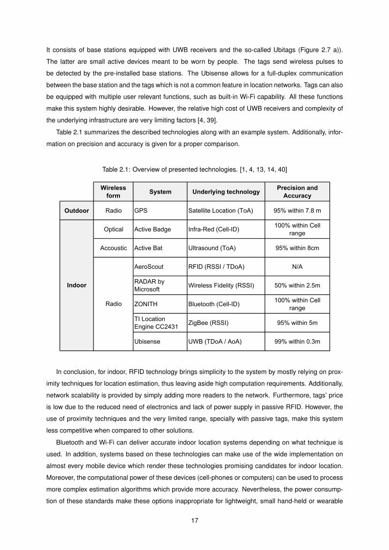
Table 21 summarizes the described technologies along with an example system Additionally infor-
mation on precision and accuracy is given for a proper comparison
Table 21 Overview of presented technologies [1 4 13 14 40]
Wireless form
System Underlying technologyPrecision and
Accuracy
Outdoor Radio GPS Satellite Location (ToA) 95 within 78 m
Optical Active Badge Infra-Red (Cell-ID)100 within Cell
range
Accoustic Active Bat Ultrasound (ToA) 95 within 8cm
AeroScout RFID (RSSI TDoA) NA
RADAR by Microsoft
Wireless Fidelity (RSSI) 50 within 25m
ZONITH Bluetooth (Cell-ID)100 within Cell
range
TI Location Engine CC2431
ZigBee (RSSI) 95 within 5m
Ubisense UWB (TDoA AoA) 99 within 03m
Indoor
Radio
In conclusion for indoor RFID technology brings simplicity to the system by mostly relying on prox-
imity techniques for location estimation thus leaving aside high computation requirements Additionally
network scalability is provided by simply adding more readers to the network Furthermore tagsrsquo price
is low due to the reduced need of electronics and lack of power supply in passive RFID However the
use of proximity techniques and the very limited range specially with passive tags make this system
less competitive when compared to other solutions
Bluetooth and Wi-Fi can deliver accurate indoor location systems depending on what technique is
used In addition systems based on these technologies can make use of the wide implementation on
almost every mobile device which render these technologies promising candidates for indoor location
Moreover the computational power of these devices (cell-phones or computers) can be used to process
more complex estimation algorithms which provide more accuracy Nevertheless the power consump-
tion of these standards make these options inappropriate for lightweight small hand-held or wearable
17
sensors
The ZigBee standard is designed for low-rate data intermittent communication which is a factor that
contributes to ultra-low power consumption of available modules In addition the mesh topology pro-
vided by the underlying protocol aids the data communication between nodes directly UWB technology
also provides a low-power solution when applied to sensor networks The use of wideband signals due
short duty-cycle pulses of UWB are able to better handle multipath effects and coupled with a low data-
rate requirements of a location system one is able to achieve a trade-off between spectral efficiency
and energy consumption [41] These solutions when compared to Bluetooth or Wi-Fi are low-power
oriented which affect the ability for a high range estimation
18
Chapter 3
Antennas for indoor location
31 Introduction
In the previous chapter the properties of location systems such as application environment location
techniques positioning algorithms underlying protocols and technologies were discussed The overall
performance of these systems also strongly depends on the properties of the antennas used as it
is the hardware element responsible for the signal emission and reception which is one of the core
components of radio-based location estimation
In this chapter the antennas designed and used for indoor location systems will be presented Im-
portant characteristics such as gain directivity radiation pattern bandwidth and polarization will be
discussed Furthermore some applications and recent developments will be exposed as well
Location techniques discussed earlier will be addressed again in this chapter First a brief techni-
cal overview of relevant properties of antennas and details will be presented Section 33 will address
antennas designed and specialized for RSSI techniques such as the dipolemonopole and printed an-
tennas In section 34 antennas for ToATDoA techniques will be discussed The details of UWB will be
analysed as it is the major technology used with this technique Finally in section 35 antennas for AoA
techniques will be explored Several examples of Smart Antennas will be presented and their properties
analysed
32 Technical overview
321 Antenna requirements
When modelling a location system special attention is required to several important details of an-
tennas that will influence their design project and final goal Antenna parameters must be chosen
adequately to satisfy location technique requirements to maximize accuracy precision and overall per-
formance These parameters can be classified as follows [42]
bull Frequency selection and bandwidth Location systems may work on different frequencies or
19
bands Antennas have to be properly adapted to the potential use of several channels as well
as impedance matched over the whole bandwidth Antenna efficiency has also to be taken into
consideration
bull Coverage Depending on the environment the system will be located in coverage requirements
are a major factor on the estimation rigour Radiation patters to study gain and directivity (ne-
cessity of ground plane or reflector for example) have to be carefully adjusted to the goals of the
application
bull Mobility User mobility has to be taken into account specially when designing antennas for mobile
unknown nodes In contrast to reference nodes mobile nodes constantly move change positions
and are much more likely to suffer damage Resilient construction materials and good protection
are required
bull Antenna position and orientation Partially also due to user mobility antennasrsquo possible working
position may constantly change This is specially relevant for mobile nodes or wearable sensors
Proper polarization mode must be chosen to minimize mismatches in the communication between
node antennas
bull Size Antenna dimensions have to be kept in view particularly for mobile nodes or even wearable
antennas whose goal is to be as small and as discrete as possible The choice for the type of
antenna should be evaluated accordingly
bull Power requirements Adaptable to the propagation environments power usage should be ad-
justed not to interfere with other systems or surpass legal requirements
bull Cost Ideally an appropriate performance-price trade-off should be found when taking into consid-
eration all of the aforementioned parameters on the design of the antennas in order to minimize
cost and maximize profitability
322 Antenna types
Antenna design diversity is introduced to enhance location system performance and robustness
These can essentially be categorized in four main groups [13] The last two groups apply only for
antennas for reference nodes
bull Omnidirectional antennas These type of antennas are primarily suited for Tri-Multilateration
techniques or Fingerprinting The lack of directivity makes these antennas independent of user
or node orientation and therefore are immune to environment changes and user mobility given a
proper polarization The coverage capability is also one of the main advantages specially due to
the reduced need of nodes
bull Directive antennas Primarily used in the scope of RFID systems for tag identification these
antennas are well suited for proximity techniques due to their narrow beam and operating range
avoiding interference with other readers
20
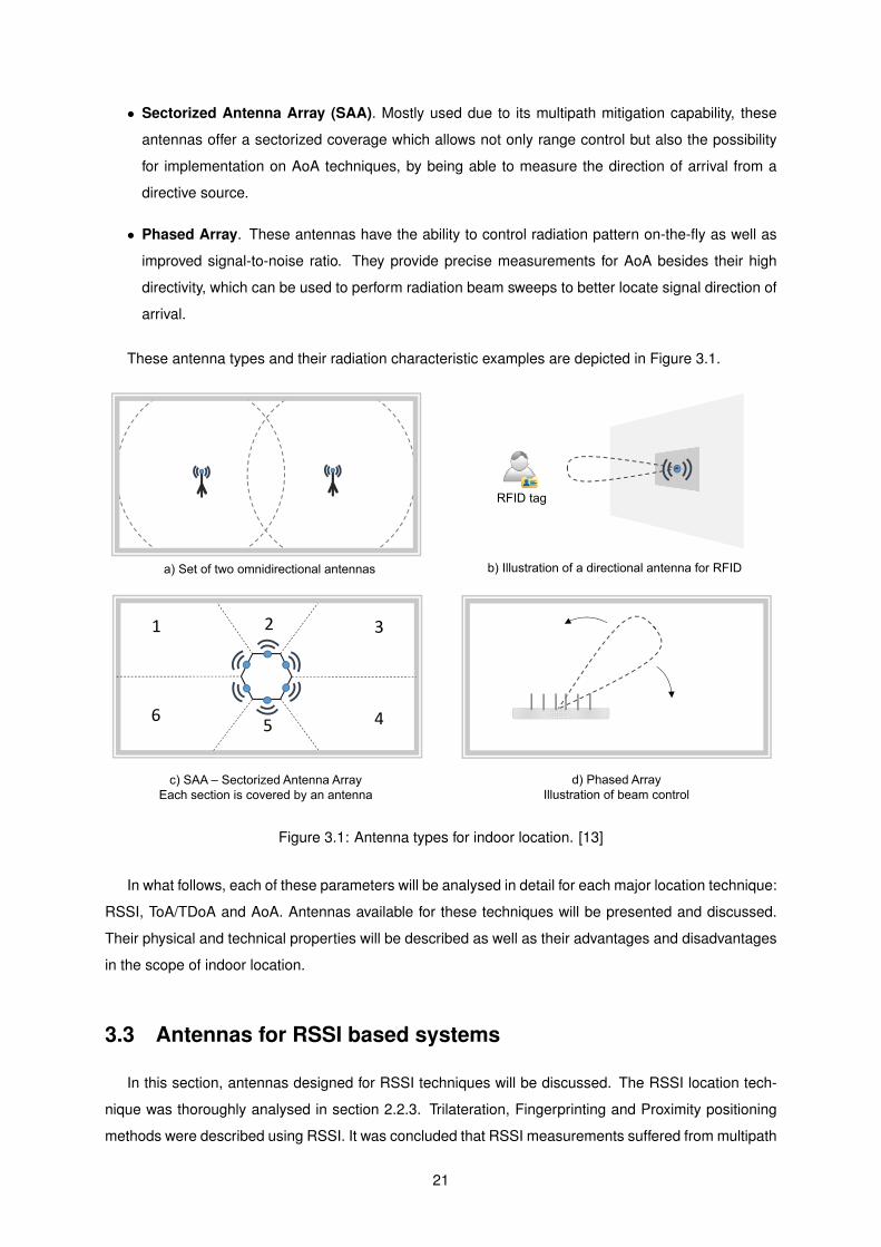
bull Sectorized Antenna Array (SAA) Mostly used due to its multipath mitigation capability these
antennas offer a sectorized coverage which allows not only range control but also the possibility
for implementation on AoA techniques by being able to measure the direction of arrival from a
directive source
bull Phased Array These antennas have the ability to control radiation pattern on-the-fly as well as
improved signal-to-noise ratio They provide precise measurements for AoA besides their high
directivity which can be used to perform radiation beam sweeps to better locate signal direction of
arrival
These antenna types and their radiation characteristic examples are depicted in Figure 31
1 2 3
456
a) Set of two omnidirectional antennas b) Illustration of a directional antenna for RFID
c) SAA ndash Sectorized Antenna ArrayEach section is covered by an antenna
d) Phased ArrayIllustration of beam control
RFID tag
Figure 31 Antenna types for indoor location [13]
In what follows each of these parameters will be analysed in detail for each major location technique
RSSI ToATDoA and AoA Antennas available for these techniques will be presented and discussed
Their physical and technical properties will be described as well as their advantages and disadvantages
in the scope of indoor location
33 Antennas for RSSI based systems
In this section antennas designed for RSSI techniques will be discussed The RSSI location tech-
nique was thoroughly analysed in section 223 Trilateration Fingerprinting and Proximity positioning
methods were described using RSSI It was concluded that RSSI measurements suffered from multipath
21
effects specially in the case of NLoS Measurement inaccuracies due to low-quality receivers and inter-
ference also influence RSSI readings As such antennas designed for this case must take into account
and try to minimize these factors
Inherent to all location systems antennas in mobile nodes are subject to continuous movement due
to user mobility Antenna placement on someonersquos body must be carefully taken into consideration This
is specially relevant for RSSI techniques that use Trilateration or Fingerprinting methods although the
latter should ideally not depend on antenna configuration given that the same antennas are used in
both on-line and off-line phases [13]
According to [13] to overcome the user mobility problem an isotropic radiative element could ideally
be implemented Thereby no orientation would be preferred against another In a real scenario however
the closest simplest element that approximates an isotropic radiator are dipoles or monolopoles Most
used solutions include the classical half-wavelength dipole or quarter-wavelength monopole due to their
omnidirectional radiation characteristic
If the bodyrsquos vertical position of a user carrying along a mobile unit is assured then relative low
motion in the elevation plane is expected This makes linear vertically polarized antennas for either
mobile nodes and reference nodes the simplest and the least expensive solution Location applications
based on RSSI primarily apply these type of antennas [13] Other solutions like collinear arrays of
half-wavelength dipoles for higher gain and directivity in the azimuthal plane are also possible
Cases where userrsquos body vertical position is not assured the use of circular polarization on the
reference nodersquos side provides robustness to the system as itrsquos taking into account possible unexpected
body movements For example in the case of antennas placed on a wrist the constant up and down
movement of the arm could compromise co-polarization between the mobile and reference node
The use of external half-wavelength dipoles commonly seen in Wi-Fi or ZigBee applications spe-
cially on the side of access points or reference nodes provides good performance and low-cost [13]
However the size of these antennas is a limiting factor for mobile applications
A more compact solution is achieved by the use of Printed Circuit Board (PCB) technology These
solutions contemplate for example the Planar Inverted-F Antenna (PIFA) or a variation of these the
Meander antennas These designs are the results of printed monopole variations Two examples from
[43] and [44] can be seen in Figure 32 a) and b) respectively
The PIFA can be seen as a monopole that was tilted towards the ground plane The proximity to the
ground plane reduces efficiency and input resistance A stub along the width of the monopole is used
to minimize this effect and so the F shape takes form This antenna is used extensively primarily due
to its simpleness good efficiency omnidirectional pattern and high gain in both vertical and horizontal
polarization modes which make this antenna appropriate for RSSI based location methods [45] The
PIFA is resonant at a quarter-wavelength and combined with its low-profile characteristic it allows for
small scale device integration which makes it a good candidate for location technologies
Another PCB antenna option is the meander antenna In this antenna the wire is folded back and
forth ie it is meandered and it can be built in a half-wavelength or quarter-wavelength monopole
format Example of the latter is depicted in Figure 32 b) By doing so the resonance frequency is
22
b) TI CC2511 USB-dongle for Wi-Fi ISM 24GHz Meander antenna
a) TI CC2430 ISM 24GHz Inverted F antenna
Figure 32 Examples of Inverted F and Meander antennas
achieved in a much more compact structure [45] The downfall towards the classical inverted F antenna
include bandwidth efficiency and input resistance drop but preserves its fairly omnidirectional radiation
pattern [46]
As discussed in section 223 proximity-based systems fix a userrsquos location by being in range of
a certain reference node or reader This is an example application for RFID technology The mobile
RFID unit or tag once itrsquos in the readerrsquos range of operation it will become associated with the location
of that reader Primarily used for authentication or stock tracking proximity based on RFID must rely on
small sized tags meaning small sized antennas and if possible planar Reduced production cost high
efficiency and reliability are also priorities Composition of RFID passive tags in its very basic contain an
RFID integrated circuit and an antenna as power source as well as for receiving and transmitting the RF
signal Due to its simplicity and low-cost dipole or dual dipole antennas are present in most Ultra-High
Frequency (UHF) RFID (300MHz to 3GHz) systems [47] In the latter case two dipoles form a cross
shape and are fed at the middle mitigating tagrsquos orientation dependency Other solution feasible for UHF
RFID Tags is the use of the already mentioned meander antennas as depicted in Figure 33
Radio Frequency Identification Fundamentals and Applications Design Methods and Solutions
98
example trimming the meander trace by ⦆x=5mm moves the resonant frequency up by 20 MHz as shown in Fig 7 The gain is not significantly affected by trimming as shown in Fig8
Fig 6 Meandered line antenna
Fig 7 Impedance of the loaded meander tag antenna (Ra Xa ) as a function of meander trace length trimming ⦆x
Fig 8 Gain of the loaded meander tag antenna in yz-plane at 900 MHz as a function of meander trace length trimming ⦆x
wwwintechopencom
Figure 33 Meander antenna for RFID Tag The additional bar and furthered meandered left sectionimproved impedance matching to the RFID chip [48]
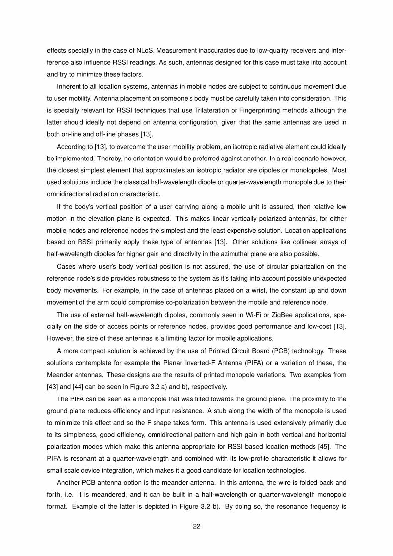
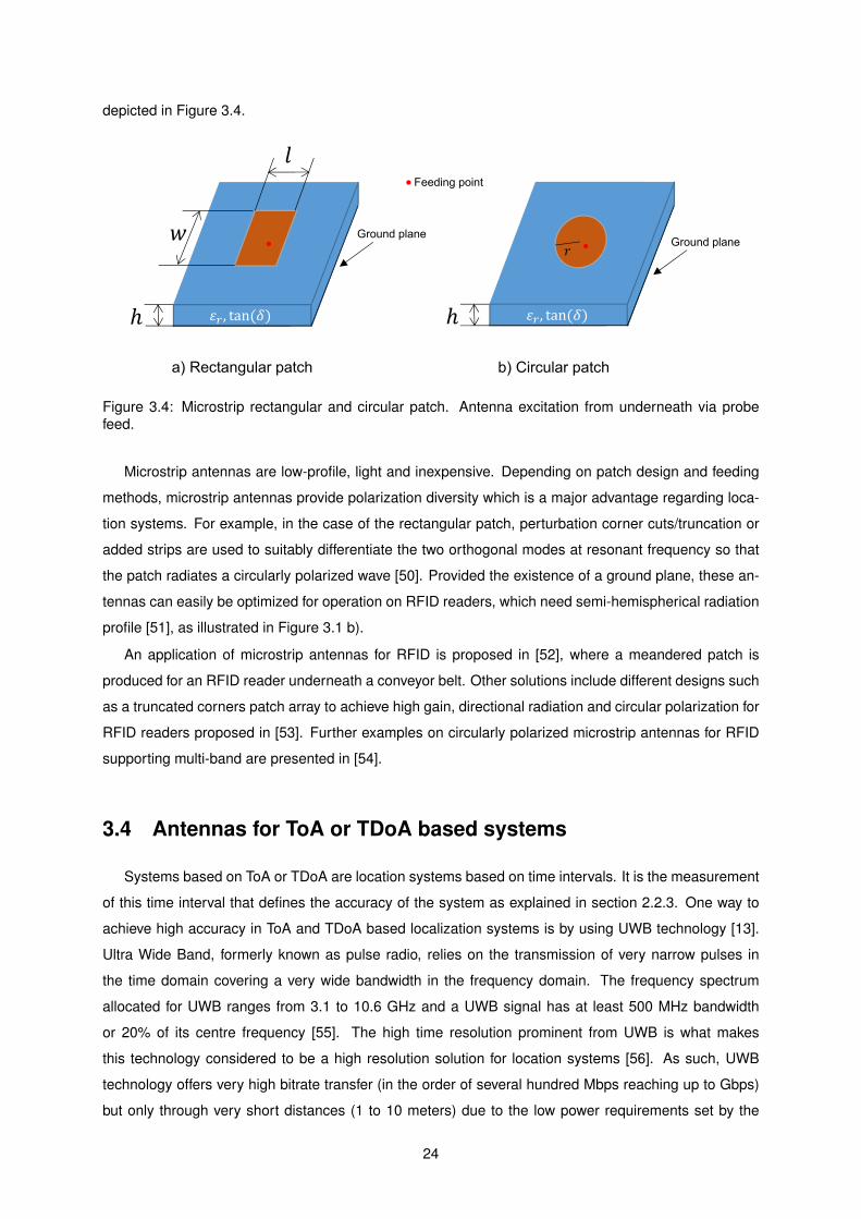
An alternative solution to the size constraint present in location systems involves the microstrip an-
tennas In its most simple form a microstrip antenna consists in a radiating element on one side of a
dielectric (relative permittivity εr and loss tangent tan(δ)) which has a ground plane on the other side
[49] The radiating elements can assume the form of rectangular circular or ring patches among oth-
ers depending on required radiation characteristics An example of a rectangular and circular patch is
23
depicted in Figure 34
tan tan
a) Rectangular patch b) Circular patch
Ground planeGround plane
Feeding point
Figure 34 Microstrip rectangular and circular patch Antenna excitation from underneath via probefeed
Microstrip antennas are low-profile light and inexpensive Depending on patch design and feeding
methods microstrip antennas provide polarization diversity which is a major advantage regarding loca-
tion systems For example in the case of the rectangular patch perturbation corner cutstruncation or
added strips are used to suitably differentiate the two orthogonal modes at resonant frequency so that
the patch radiates a circularly polarized wave [50] Provided the existence of a ground plane these an-
tennas can easily be optimized for operation on RFID readers which need semi-hemispherical radiation
profile [51] as illustrated in Figure 31 b)
An application of microstrip antennas for RFID is proposed in [52] where a meandered patch is
produced for an RFID reader underneath a conveyor belt Other solutions include different designs such
as a truncated corners patch array to achieve high gain directional radiation and circular polarization for
RFID readers proposed in [53] Further examples on circularly polarized microstrip antennas for RFID
supporting multi-band are presented in [54]
34 Antennas for ToA or TDoA based systems
Systems based on ToA or TDoA are location systems based on time intervals It is the measurement
of this time interval that defines the accuracy of the system as explained in section 223 One way to
achieve high accuracy in ToA and TDoA based localization systems is by using UWB technology [13]
Ultra Wide Band formerly known as pulse radio relies on the transmission of very narrow pulses in
the time domain covering a very wide bandwidth in the frequency domain The frequency spectrum
allocated for UWB ranges from 31 to 106 GHz and a UWB signal has at least 500 MHz bandwidth
or 20 of its centre frequency [55] The high time resolution prominent from UWB is what makes
this technology considered to be a high resolution solution for location systems [56] As such UWB
technology offers very high bitrate transfer (in the order of several hundred Mbps reaching up to Gbps)
but only through very short distances (1 to 10 meters) due to the low power requirements set by the
24
Federal Communications Commission and the European Telecommunications Standards Institute as
not to cause unwanted interference to devices operating on the same band Moreover UWB signals
present relative immunity to multipath effects due to reduced signal overlap at the receiver and grant an
extremely fine time and range solution even through opaque media [55]
Overall ToA estimation with or without UWB is influenced by the following common error sources
[71]
bull Multipath effects Indoor environments are specially susceptible to multipath effects due to the
high obstacle density between transmitter and receiver A transmitted pulse in a narrowband sys-
tem overlaps with other multipath originating copies at the receiver In the case of correlator
receiver this effect causes a shift in the correlation peak and introduces a large estimation error
High computational effort has to be employed to mitigate these effects with the help of super-
resolution techniques [57] The short duration of UWB pulses avoids the need for such computa-
tional requirements as the pulse duration is much shorter than the interval of arrival of the multipath
components
bull Interference Interference in a multiuser environment (or in a multinode environment in the case
of a location system) can impose severe limitations Multiple access techniques like time slot
attribution or frequency band allocation can help mitigate interference
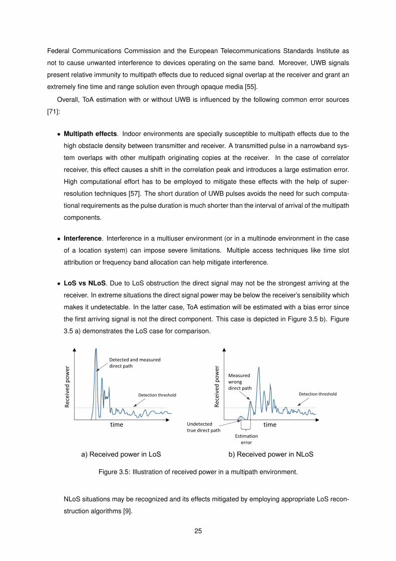
bull LoS vs NLoS Due to LoS obstruction the direct signal may not be the strongest arriving at the
receiver In extreme situations the direct signal power may be below the receiverrsquos sensibility which
makes it undetectable In the latter case ToA estimation will be estimated with a bias error since
the first arriving signal is not the direct component This case is depicted in Figure 35 b) Figure
35 a) demonstrates the LoS case for comparison
time
Received
power
timeUndetectedtrue direct path
Detection thresholdDetection threshold
Detected and measureddirect path
Measuredwrongdirect path
Received
power
Estimationerror
a) Received power in LoS b) Received power in NLoS
Figure 35 Illustration of received power in a multipath environment
NLoS situations may be recognized and its effects mitigated by employing appropriate LoS recon-
struction algorithms [9]
25
bull High-time resolution of UWB signals Due to the short UWB pulse duration nodersquos clock syn-
chronization jitter plays a role in ToA estimation errors Also a low sampling rate is required to
achieve a low power design [25]
Besides the requirements mentioned in section 321 the design of UWB antennas must consider
the following aspects according to [13]
bull Bandwidth For conventional UWB antennas must present a minimum 500 MHz operational
bandwidth For robustness the antennas should ideally cover the entire UWB band
bull Radiation patten Similar to antennas for RSSI based location UWB antennas should possess a
high omnidirectional radiation pattern
bull Operation uniformity The antennas should operate uniformly throughout the entire operational
bandwidth A stable phase centre at all operation frequencies is required as not to deform the
shape of UWB pulses [58]
bull Dimensions and cost UWB antennas should be planar and have low-profile characteristics to
allow small device integration and the lowest cost
bull Radiation efficiency Due to the low power nature of UWB technology antennas must present
high efficiency Typically greater than 70 [13]
bull Linear phase Coupled with operation uniformity over the total bandwidth phase response of
antennas for UWB should be a linear function of the frequency as not to distort the shape of UWB
pulses
Antennas for ToA or TDoA with UWB technology share many of the required characteristics with
antennas for RSSI As such there are many proposed designs for UWB antennas fulfilling these re-
quirements [59ndash66] In the past horn structures crossed or rolled antennas were developed for UWB
applications However these structures did not meet the low-profile requirements for small scale integra-
tion despite their high bandwidth and omnidirectional radiation pattern required for ToA or TDoA based
localization systems [60] To overcome this problem PCB solutions are implemented A typical design
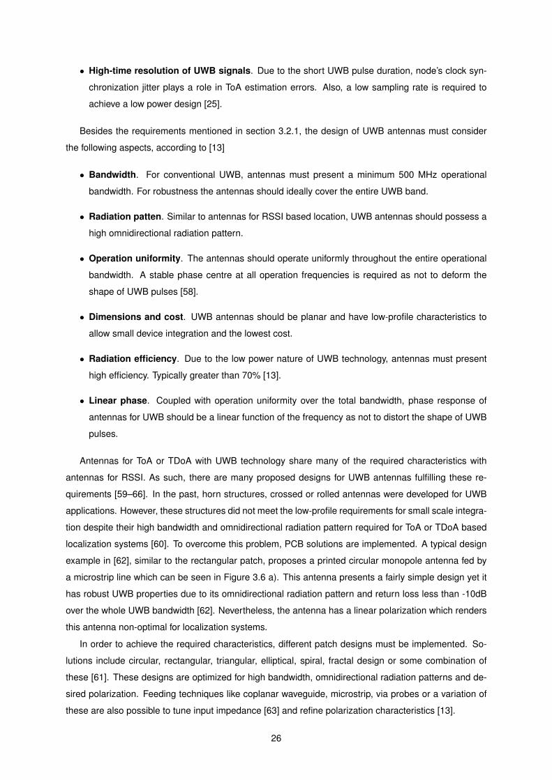
example in [62] similar to the rectangular patch proposes a printed circular monopole antenna fed by
a microstrip line which can be seen in Figure 36 a) This antenna presents a fairly simple design yet it
has robust UWB properties due to its omnidirectional radiation pattern and return loss less than -10dB
over the whole UWB bandwidth [62] Nevertheless the antenna has a linear polarization which renders
this antenna non-optimal for localization systems
In order to achieve the required characteristics different patch designs must be implemented So-
lutions include circular rectangular triangular elliptical spiral fractal design or some combination of
these [61] These designs are optimized for high bandwidth omnidirectional radiation patterns and de-
sired polarization Feeding techniques like coplanar waveguide microstrip via probes or a variation of
these are also possible to tune input impedance [63] and refine polarization characteristics [13]
26
Ground plane Ground plane
Microstrip feeding line Microstrip feeding line
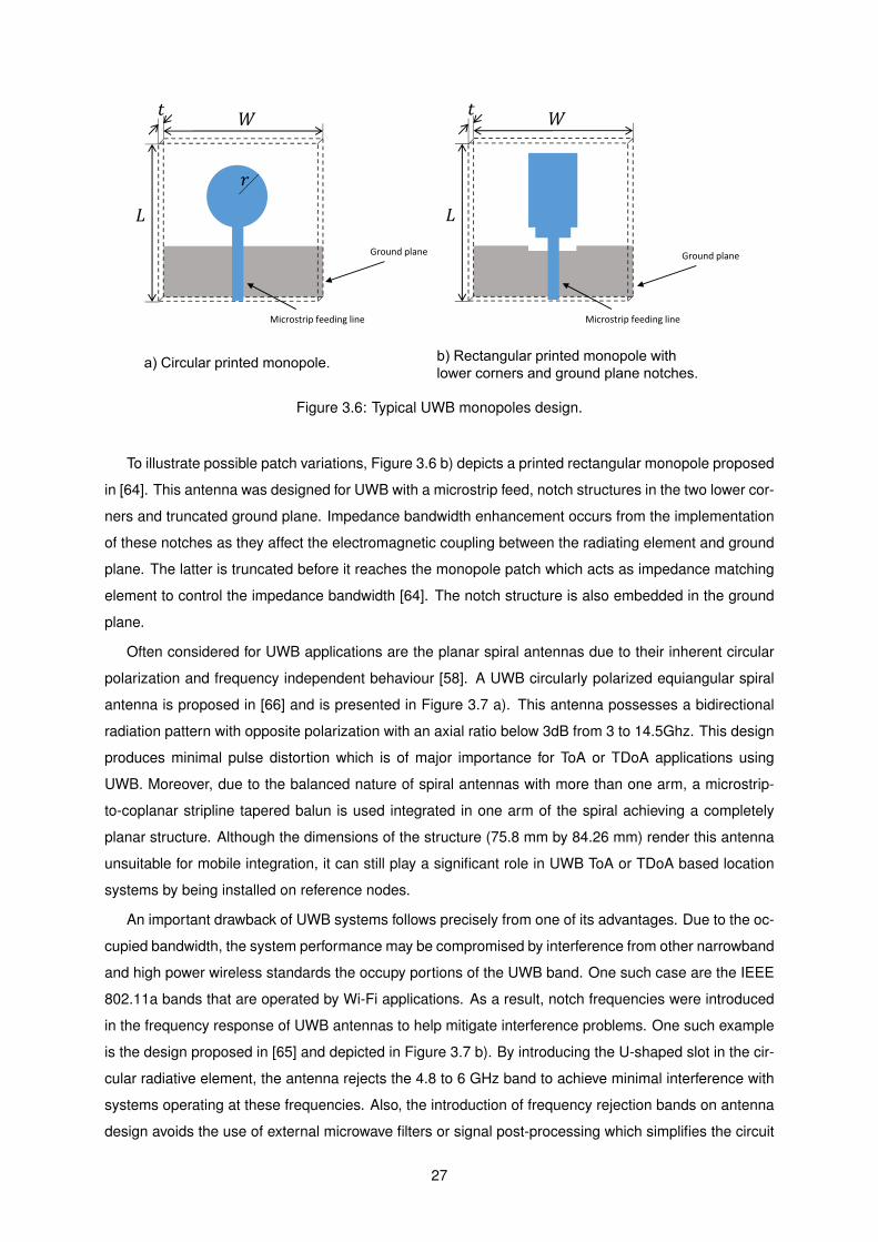
a) Circular printed monopole b) Rectangular printed monopole withlower corners and ground plane notches
Figure 36 Typical UWB monopoles design
To illustrate possible patch variations Figure 36 b) depicts a printed rectangular monopole proposed
in [64] This antenna was designed for UWB with a microstrip feed notch structures in the two lower cor-
ners and truncated ground plane Impedance bandwidth enhancement occurs from the implementation
of these notches as they affect the electromagnetic coupling between the radiating element and ground
plane The latter is truncated before it reaches the monopole patch which acts as impedance matching
element to control the impedance bandwidth [64] The notch structure is also embedded in the ground
plane
Often considered for UWB applications are the planar spiral antennas due to their inherent circular
polarization and frequency independent behaviour [58] A UWB circularly polarized equiangular spiral
antenna is proposed in [66] and is presented in Figure 37 a) This antenna possesses a bidirectional
radiation pattern with opposite polarization with an axial ratio below 3dB from 3 to 145Ghz This design
produces minimal pulse distortion which is of major importance for ToA or TDoA applications using
UWB Moreover due to the balanced nature of spiral antennas with more than one arm a microstrip-
to-coplanar stripline tapered balun is used integrated in one arm of the spiral achieving a completely
planar structure Although the dimensions of the structure (758 mm by 8426 mm) render this antenna
unsuitable for mobile integration it can still play a significant role in UWB ToA or TDoA based location
systems by being installed on reference nodes
An important drawback of UWB systems follows precisely from one of its advantages Due to the oc-
cupied bandwidth the system performance may be compromised by interference from other narrowband
and high power wireless standards the occupy portions of the UWB band One such case are the IEEE
80211a bands that are operated by Wi-Fi applications As a result notch frequencies were introduced
in the frequency response of UWB antennas to help mitigate interference problems One such example
is the design proposed in [65] and depicted in Figure 37 b) By introducing the U-shaped slot in the cir-
cular radiative element the antenna rejects the 48 to 6 GHz band to achieve minimal interference with
systems operating at these frequencies Also the introduction of frequency rejection bands on antenna
design avoids the use of external microwave filters or signal post-processing which simplifies the circuit
27
a) Circularly polarized printed monopole b) Circularly polarized spiral antenna
Figure 37 Illustration of two UWB circularly polarized antennas
and allows substantial size and cost reduction of the overall module [61]
Another solution to reduce the effect of interference sources and to be able to control the rejection
bands more easily relies on the so-called dielectric loading sandwich technique [67] A padding patch
printed on a substrate layer is glued on top of the radiative element of the UWB antenna This procedure
is depicted in Figure 38
Figure 38 Depiction of the dielectric loading sandwich technique [67]
The upper and lower semicircles resonate at one distinct frequency respectively The existent
padding patch causes destructive interference at these two frequencies and so two separate notches
occur in the frequency response of the antenna Additionally the notch bandwidth can be controlled by
varying the substrate thickness of the padding patch
35 Antennas for AoA based systems
In systems based on AoA measurements the angle or direction of arrival of a signal transmitter
from an unknown node is estimated These estimations are performed by implementing antenna ar-
rays or directional antennas Their configuration will allow the system to achieve the desired accuracy
28
connectivity and spectral efficiency [13]
Measuring the angle of arrival of a signal on a reference node is far more complex than the previous
location estimation options Antennas developed for this purpose occupy more space when compared
to other techniques due to the need of arrays or more than one antenna to cover certain regions in a
3D space Additionally a fixed space reference for accurate location estimation is needed As such
antennas developed for AoA systems are placed in base station or reference nodes where user mobility
is not required
The Smart Antennas have been an emerging technology to cover AoA estimation necessities [29]
These antennas provide the possibility to control some of its properties like polarization and radiation
pattern in real time Included in this group are the SAA [29 30 68] and Phased Arrays [69ndash71] The
former consists of a set of directional antennas oriented in such a way for each to cover a certain solid
angle achieving a distributed coverage of the space The latter consists in a antenna array where the
phase of the signals is controlled in such a way as to re-enforce the radiated energy in a desired direction
and to cancel in others Phased arrays also allow other forms of beam control which will be discussed
later on
With this is mind the development of antennas for AoA estimation the following aspects must be
taken into consideration [29]
bull Position An unobtrusive position to the users is desired to minimize visual and spatial impact
The antenna should be placed preferably in the centre of the covered room in order to achieve
maximum coverage and reduce dark spots
bull Interference In dense networks where several systems may be working on the same frequency
bands spatial selectivity is advised for interference reduction
bull Spatial arrangement The spatial arrangement of the antennas constituting the array should
maximize 3D space coverage preferably equally and enable spatial re-usability In the case of
SAA antenna coupling should be reduced as not to deform the radiation pattern
bull Radiation pattern Depending on the antenna type and coupled with spatial arrangement anten-
nas for AoA should be able to receive and send signals almost isotropically
bull Polarization AoA estimation is heavily affected by multipath effects It has been referred to in the
literature that circular polarization for these antennas can help mitigate these effects [29]
bull Cost Antenna design should take into account the network topology and operation environment
To achieve low-cost production PCB antennas should be preferred
A Smart Antenna and system for location-aware applications is proposed in [29] The structure of
the antenna can be seen in Figure 39 a)
This antenna is composed of six equal circularly polarized printed antennas placed on the surfaces
of a half dodecahedron intended to be mounted on the ceiling to provide 3D space coverage This is a
29
a) Switched beam antenna b) Sectorized Antenna Array for UWB
Figure 39 Examples of smart antennas design
switched beam sectorized antenna array and narrowband system where each radiating element is se-
lected by a multiplexing circuit This antenna allows 2D location estimation by providing both the azimuth
and elevation angles of the incoming signal RSSI readings on each antenna provide the necessary in-
formation for the array signal processing algorithm in this case the MUSIC algorithm [27] to estimate
the angle of arrival Performance tests showed that this system can estimate a location with an average
error of 17m [29]
UWB solutions are also present in AoA estimation Antenna requirements for these systems are
similar to those for UWB in ToA estimation [13] In [30] a UWB antenna and hybrid AoAToA system for
high accuracy positioning is proposed An hexagonal monopole antenna array of six elements facing
different directions is used for omnidirectional coverage The antenna is depicted in Figure 39 b) The
proposed system estimates the angles of arrival based on amplitude difference of the tag reflected
UWB pulse arriving at the different array antennas similar to the mono-pulse radar operation Due to
the ease of signal amplitude measurements and the high precision provided by UWB technology as
discussed earlier this system can achieve an accuracy up to 2cm proving how well hybrid solutions
such as AoAToA perform Similar to this concept another solution presented in [72] which proposes
a cylindrical conformal array of UWB antennas to achieve the same goal The proposed antenna is
depicted in Figure 310
Figure 310 Cylindrical conformal array of UWB Antennas [72]
30
Chapter 4
Development of a reflector UWB
Antenna
In this chapter a UWB antenna to be used in the developed localization system is proposed First
basic concepts like antenna type and its relevance are introduced In section 42 the antenna design
is described along with parameter optimization Then in section 43 the test results of the antenna
prototype are presented At last in section 44 some conclusions are drawn related to the design and
antenna testing phase
41 Introduction
As previously discussed in Chapter 3 printed UWB antennas have been of major importance lately
due to their wideband characteristic low cost and reduced dimensions In this chapter a UWB antenna is
proposed taking advantage of its properties for implementation on an RTLS system The RTLS system
for which the antenna is designed consists of four identical hardware PulsOn P400 active modules from
Time Domain which perform ranging measurements With four available modules the RTLS system is
composed of three static base stations and one free target
The original stock antennas (Figure 41) for each module are variations of a UWB monopole which
offers a nominal 3dBi gain in all directions perpendicular to the antenna This omnidirectional radiation
characteristic is optimal when orientation of the target is not known or when signals are expected to
arrive from any direction which is the case However for static base station antennas their spacial
orientation can be set and remain unchanged throughout the operation of the system Consequently
a UWB monopole may not be the optimal antenna for a static base station if the target remains in a
confined area To improve Signal-to-Noise ratio (SNR) and possibly decrease measurement variance
a more directional and high gain antenna is developed and tested Additionally the more directivity the
less multipath effects on received and sent signals
The main idea behind the development of the proposed high gain directive UWB antenna relies on
the use of a reflector metallic plane placed near the antenna so that the radiated power can be narrowed
31
Figure 41 Stock UWB monopole variation
down to a specific direction Different reflector plane distances to the antenna will be tested to achieve
best impedance matching and maximize directivity particularly for the 31 to 53GHz band which is the
P400 module working frequency
42 Antenna Design
421 Base model
There are many printed antenna designs for UWB applications Several examples were discussed in
section 35 some of which include spiral monopole or slot antennas The choice for the antenna design
relies on its desired radiation characteristics which are formalized below for the RTLS system developed
in this work
bull Directivity and Gain Antenna application requires high directivity to maximize radiated power in
the spatial direction of interest In this case the antenna is designed to achieve maximum possible
directivity in the z direction (see Figure 42)
bull Polarization The developed RTLS system is designed to perform on a 2D plane which includes
base stations and target antennas Therefore circular polarization is not a requirement Besides
the target antenna is linearly polarized As such to avoid polarization mismatches the proposed
antenna is designed to be linearly polarized as well
bull Impedance matching A common impedance matching criterion is
PrPi le 01 (41)
where Pr is the reflected power and Pi is the incident power The last equation can be described
in terms of the antenna reflection coefficient which can be expressed by the scattering parameter
S11
|S11| le minus10dB (42)
The proposed antenna is designed to have the S11 parameter below the threshold in the frequency
band of interest (31 to 53 GHz)
32
The printed antenna design is inspired by the monopole design depicted in Figure 36 However
to better control geometrical dimensions of the antenna without making it too large as well as to keep
metallic surface as small as possible to minimize losses the upper half of the circumference was left
out The start design point is depicted in Figure 42 Also an inverted triangle was cut out on the top of
the stub to compensate for surface current path on lower frequencies Its effect will be parametrized and
analysed to find the optimal dimensions in order to achieve the best impedance matching
W = 48
L = 43
Vc
dtat
s=4
we
u = 085
P = 17
dg = 08
y
xz
Figure 42 Base model for the proposed UWB antenna design - reflector plane and SMA connector notshown (dimentions in mm)
As it is shown in Figure 42 the antenna is fed by a Coplanar Waveguide (CPW) In this feeding
technique the ground conductors and the feed line are on the same plane The substrate used is the
Rogers 5880 laminate with 0787mm thickness and dielectric constant εr = 22 All metallic parts and
surfaces (conductors connector and reflector plane) are modelled by lossy copper with conductivity
58times107 Sm The software tool used to simulate antenna behaviour is the CST Microwave Studio 2015
and the model produced in this software is depicted in Figure 43 The connector model is shown in
Appendix A
The distance from the reflector plane to the antenna is λc4 where λc if the wavelength correspondent
to the centre frequency (fc = 43Ghz) of the band of interest
λc4 =c
4fc=
2998times 108
4times 43times 109mm = 1743mm (43)
The parameter m is added to the distance λc4 and is initially assumed to be zero In order to observe
the influence on the scattering parameter S11 of the distance from the antenna to the reflector plane
a sweep on this parameter will be carried out together with the parameters at we and vc - all other
parameters remain constant
33
y
zx
y
zx
L + 2alt
alt
1743+m
alt
Perspective view Side view
Figure 43 Perspective and side view of the antenna model with reflector plane and SMA connector(dimensions in mm)
422 Parameter analysis
In Figure 44 a parameter sweep of we is carried out between 01 and 06mm in a 05mm step where
at = m = 0mm vc = 2145mm and alt = 10mm It can be concluded that we = 05mm leads to an S11
below -10dB for the band 25-55GHz and produces a significant resonance at 38GHz
Figure 44 Sweep for the parameter we Left S11 in dB Right Directivity in dBi
Next a sweep on the m was performed between -1 and 2mm The other parameters were kept
constant we = 05mm at = m = 0mm and vc = 2145mm The result is depicted in Figure 45 It can
be observed that the best impedance matching for the whole band is found at m = minus1mm which makes
this the value chosen for m
Additionally a sweep was performed on the parameter at The result is depicted in Figure 46 It can
be concluded that the cut out triangle on the metallic surface of the antenna with height at has a little
influence on the reflection coefficient S11 However despite the minor influence the value at = 1185mm
is adopted as it still minimizes S11
Moreover a sweep on the radius vc was performed The results are presented in Figure 47 It
34
Figure 45 Sweep for the parameter m Left S11 in dB Right Directivity in dBi
Figure 46 Sweep for the parameter at Left S11 in dB Right Directivity in dBi
Figure 47 Sweep for the parameter vc Left S11 in dB Right Directivity in dBi
can be concluded that this parameter has a strong influence on the reflection coefficient Such an
effect was expectable since the physical properties of region where the surface current is high are being
changed namely the gap between the ground and the stub Furthermore taking into account the Gain
dependency depicted in Figure 47 the value vc = 2333mm was chosen for this parameter
In addition the effect on reflector height alt was investigated The results can been seen in Figure
35
48
Figure 48 Sweep for the parameter alt Left S11 in dB Right Directivity in dBi
Analysing Figure 48 clearly the best result in terms of S11 and Directivity stability is achieved when
alt = 20mm However this would mean a reflector plane 4cm longer than the actual antenna A fair
compromise can be found setting alt = 10mm
Finally the influence of reflector incline was analysed Figure 49 depicts the various possible re-
flector positions depending on the angle α The results of the performed sweep can be seen in Figure
410
y
zxL + 2alt
alt
1743+m
alt
Side view
α
α(L + 2alt) 2
Figure 49 Reflector inclination dependent on angle α
From Figure 410 it can be concluded that there is no significant influence of α on the reflection
coefficient Although it does change antenna directivity the manufacturing process requires an additional
step which is to make sure the reflection plane is placed at the right angle This step will introduce errors
which are in order of magnitude of the optimal angle (α = minus10) compromising the optimization As
such the reflector plane remains parallel to the antenna substrate (α = 0)
The Directivity and the reflection coefficient S11 for the chosen parameters are depicted in Figure
36
Figure 410 Sweep for the parameter α Left S11 in dB Right Directivity in dBi
411 for the band 2-10Ghz
Figure 411 S11 and Directivity for the final parameters
Although the antenna has been optimized to work in the band 31-53GHz it can been seen from
Figure 411 that the antenna completely fulfils impedance matching requirements up to 10GHz meaning
that it allows applications that work outside the range of frequencies the antenna was originally designed
for Nevertheless from Figure 411 it can be concluded that above 6GHz the antenna ceases to be
directive in the z direction and is no longer optimal for ranging applications Radiation patterns for the
frequencies 31 43 and 53GHz are presented in Appendix B
43 Performance Analysis
A prototype of the developed antenna model was produced so that it could be tested in a real world
scenario The substrate and connector used were the same as the simulated materials To build the
reflector plane a rectangular piece of brass was cut and fastened to a block of Roofmate Styrofoam
The good electrical properties (εr asymp 1) and lightness of this material make it a good option to emulate an
air gap between the reflector and the substrate which was placed in the opposite side of the block This
Styrofoam block also acts as solid structure to hold the prototype parts in place A picture of the finished
37
prototype is presented in Figure 412
Figure 412 Antenna prototype
Two procedures are carried out in this performance analysis First the antenna reflection coefficient
S11 is measured to obtain impedance matching data Lastly the prototype is tested in the scope of a
ranging system specifically distance measurement with the PulsOn P400 modules from TimeDomain
which are also the hardware building blocks of the indoor localization system developed in this work
431 Measurement of reflection coefficient
To perform impedance matching measurements the prototype antenna was connected to the Vector
Network Analyser (VNA) E5071C of Agilent Technologies and placed on top of absorbent material to
minimize reflections Also to help mitigate coaxial cable effects a strip of absorbent material was
wrapped around the cable near the connector Measurement set-up is depicted is Figure 413
Figure 413 S11 measurement
A frequency sweep from 2GHz to 10GHz was conducted and the S11 results are plotted in Figure
414
By analysing the obtained results it can be concluded that the antenna is matched for the band
33GHz to 10GHz which corresponds to the simulated results except for the lower frequencies The
38
Frequency GHz2 3 4 5 6 7 8 9 10
S11
dB
-60
-50
-40
-30
-20
-10
0
Simulated S11Measured S11
Figure 414 S11 measurement and simulated results
lower band of the prototype in contrast to the theoretical model can be explained by several factors
not accounted for in the simulation First it can be seen in Figure 45 that good impedance matching
is highly sensible to the distance between the substrate and the reflector The sub-millimetre precision
required to get optimal experimental results cannot be reached in practice therefore the results are
subject to error Moreover coaxial cable to connector mismatch will affect input impedance which will
in turn worsen S11 results Furthermore substrate misalignments relative to the ground plane will also
negatively influence results
At the beginning of the band of interest (31GHz) the antenna prototype as an S11 equal to -75dB
which is an acceptable value nonetheless Additionally the prototype still has very favourable expected
directivity This fact makes it a good candidate for ranging applications which will be tested next
432 Performance measurement in a ranging system
To evaluate performance in a real ranging system three PulsOn P400 modules were used One
target and two base stations The proposed antenna was attached to one of the base stations The
other two modules use the stock 3dBi omni-directional monopole antenna [73] which will act as the
reference antenna The measurement set-up is depicted in Figure 415 A picture of base station nodes
is also presented in Figure 416
moduleBS
moduleBS
reference antenna
proposedantenna
moduleTarget
reference antenna
mobile
fixed
Figure 415 Measurement scheme
39
The objective of this test is to compare distance measurement variance between antennas as well as
to obverse the change in RSSI for both base stations To achieve this 1000 distance samples between
the target and the base stations were taken in 03m steps from 06m to 48m Measurement variance
was computed and plotted in Figure 417
Ref antenna
Proposed antenna
Figure 416 Picture of reference and proposed antenna on their respective nodes
Distance m0 1 2 3 4 5
Sta
ndar
d D
evia
tion
mm
0
10
20
30
40
50
60
70
Proposed antennaReference antenna
Figure 417 Standard deviation for proposed andreference antenna
Distance m0 1 2 3 4 5
RS
SI d
iffer
ence
dB
-10
-8
-6
-4
-2
0
2
4
6
8
10
Figure 418 RSSI difference between proposedand reference antenna
In can be seen that the proposed antenna manages to slightly improve measurement variance spe-
cially for small distances when compared to the reference antenna In Figure 418 the difference in
RSSI in dB from both base stations is plotted It can be seen that although both antennas perform
similarly in terms of measurement variance the proposed antenna improves RSSI at the target up to
33dB On average RSSI increases 227dB This result indicates system range improvement as well as
higher capability and compatibility for application in RSSI based localization systems
It is worth to mention that the presented results only apply for the commercial system in study
Performance may vary if the proposed antenna is used in other systems This is because signal post-
processing algorithms vary from system to system In this specific case they are not known to the user
and they too have influence on measurement variance Moreover UWB pulse distortion caused by the
40
antenna will also affect variance results - antenna fidelity factor [74] measurements were not carried out
due to time constraints
44 Summary
A new UWB antenna with reflector has been proposed for UWB ranging applications to replace the
omni-directional 3dBi stock antennas provided in the commercial set of Time Domain P400 modules
This new antenna makes use of a reflector plane whose angle and distance was studied to maximize
directivity in the z direction Moreover the antenna is matched up to 10GHz which can be of interest for
other applications outside the band of interest to this work (31 - 53GHz) However the radiation pattern
is not optimized for frequencies above 53GHz
One example of the application environment for this antenna consists on its use for localization
system in active base stations located on the same plane as the target The high directivity of the
proposed antennas illuminates only a certain and well defined region of space concentrating the radiated
power in a specific direction and at the same time mitigating the effects of other multipath signals
arriving from other directions
The prototype of the proposed antenna was fabricated and put under test First the reflection coeffi-
cient S11 was measured It could be observed that in the lower frequencies the antenna was above the
-10dB threshold which can be caused by manufacturing imperfections and connector mismatch issues
However from 33 up to 10GHz the antenna is matched as expected Lastly the prototype was attached
to one ranging module acting as base station for measurement variance comparison with the stock 3dBi
omni-directional antennas for this system A slight improvement has been observed specially for short
distances Moreover the difference RSSI was computed It has been concluded that the proposed an-
tenna increases RSSI at the target up to 33dB which can improve system range and compatibility with
RSSI based localization systems
41
42
Chapter 5
Location techniques and solvers
Distance measuring in real-word localization scenarios is subject to inaccuracies that require the
use of algorithms that try to mitigate the effects of errors in the measurements and deliver the best
approximate result The software developed in this work makes use of these algorithms to process
target position estimation The challenge is to find the most appropriate method to solve the following
non-linear and (possibly) overdetermined system of equations that describes ToA localization
di(x y) =radic
(xminus xi)2 + (y minus yi)2 + εi i = 1 2 M (51)
where di is the measured distance M is the number of measurements (often coincides with the
number of base stations) (xi yi) are the coordinates of the i-th reference node and εi is the measure-
ment error or the residual The parameter processed by the algorithms in the developed software is the
measured distance di and not the ToA itself - however the two only differ by the factor c the speed of
light so the problem formulation remains unchanged
Computational performance and accuracy are two ideal concepts that are unfortunately at opposite
sides of the spectrum and are as such impossible to achieve simultaneously A trade-off between these
two essential goals has to be found based on the systemrsquos needs Based on the research conducted in
Chapter 2 the algorithms can be separated into two main categories
bull Linear approach Typically involves linearized versions of the Least Squares method which pro-
duces fast results with a minimum of mathematical operations although not guaranteed to be near
the correct result Improved versions take into account the variance of the measurements to pro-
duce a Linear Weighted Least Squares problem which are discussed in this work Further linear
methods are also mentioned in section 512
bull Non-linear approach Non-linear approaches generally involve iterative algorithms that may reach
the correct solution to the non-linear problem within a few steps given proper initialization which
can be done by implementing a previous linear approach Although accurate to the desired pre-
cision level these algorithms are computationally intensive Further characteristics on iterative
algorithms are detailed in section 521
43
The software developed in scope of this work makes use of the aforementioned Linear and Non-
Linear approaches to estimate target position In this section the mathematical models for the methods
used to estimate target localization are presented along with the proper modifications for implementation
on an indoor Real-Time Localization System
51 Linear Approaches
511 Simple Geometric Pinpoint
The SGP is a simple and direct positioning method For three base stations the case of interest the
SGP consists in finding the target position based on the centroid of the triangular shape formed by the
three most closed points known as cluster points corresponding to the intersection of the range circles
provident from a ToA based range estimation Figure 51 depicts the location of the target node (black
cross) cluster points (red) and ToA circles for two intersection scenarios
a) Evey ToA circle intersects one another
b) At least one pair doesnrsquot intersect one another
Figure 51 Cluster of ToA estimation
The intersection points of two ToA circles are obtained by solving the following system of equations
r21 = (xminus x1)2 + (y minus y1)2
r22 = (xminus x2)2 + (y minus y2)2
Where (x1 y1) and (x2 y2) are base station coordinates and r1 and r2 are distance estimates to
target The solution set (xc1 yc1) (xc2 yc2) exists when both circles intersect and both points are candi-
dates to cluster points Figure 51 a) To determine which of the two intersections belongs to the cluster
the distance differences from the two intersection points to the circle defined by the measurement of
the third base station are computed The point whose distance difference is the smallest belongs to the
cluster In case the ToA circles only intersect at one point there is only one solution to the system of
equations and the corresponding point (xc yc) is automatically a cluster point The third case Figure
51 b) occurs when two ToA circles donrsquot intersect at all In this case the cluster point is a point where
the distance to either circles is minimized
The centroid of the triangle formed by the cluster points can be found by averaging the x and y
coordinates of the cluster points Let xc1 xc2 xc3 and yc1 yc2 yc3 be the x and y coordinates of the
44
cluster points respectively Then the centroid denoting target final position (xT yT ) is
xT =xc1 + xc2 + xc3
3yT =
yc1 + yc2 + yc33
The SGP can be applied to any system where the Base Station (BS) number is larger than 1 and
is useful for course localization measurements that donrsquot require much accuracy The fact that it has
a closed form solution makes this a low resource method which is favourable for computation time
The points provided through SGP may serve as initialization points for more advanced and computer
intensive statistical approaches like Least Squares (LS) Still it is not guaranteed that SGP points will
be close to the optimal LS solution which can increase computational requirements compared to other
initialization techniques This issue is addressed in the next section where linear and non-linear least
squares approximations are presented
512 Linearized Least Squares Approximation
Linear solutions consist on modifying the involved equations so that they depend linearly on the
parameters to be estimated in this case x and y the coordinates of the target position To begin with
ToA is employed so the non-linear equation system is as follows
cti = di = fi(x y) + εi i = 1 2 M (52)
where di is the estimated distance between the target node and the i-th reference node ti is the actual
ToA measurement c is the speed of light εi denotes the measurement error residual or noise and
fi(x y) =radic
(xminus xi)2 + (y minus yi)2 i = 1 2 M
Following the linearization proposed in [75] squaring both sides of (52) gives
xxi + yyi minus1
2R2 =
1
2(x2i + y2
i minus f2i ) i = 1 2 M (53)
with R =radicx2 + y2
Writing the system of equations in (53) in the matricial form A~γ = ~b
A =
x1 y1 minus 1
2
x2 y2 minus 12
xM yM minus 12
~γ =
x
y
R2
~b =1
2
x2
1 + y21 minus f2
1
x22 + y2
2 minus f22
x2M + y2
M minus f2M
The system
A~γ = ~b (54)
45
can be solved recurring to the known standard least squares estimation
~γ = argmin~γ
(A~γ minus~b)T (A~γ minus~b) = (ATA)minus1AT~b (55)
In case there are only three measurements (one from each base station ie M = 3) the system in
(54) is determined and has a trivial solution which is given by
~γ = Aminus1~b (56)
Although simple the method in (55) still has two problems First the restriction R =radicx2 + y2 is
not accounted for and secondly in case M gt 3 the variance of the errors σ2i is also ignored The latter
means that independent of variance all measurements will have the same weight on determining the
final LS solution Also the value of fi is unknown and will have to be replaced by di for implementation
To improve the estimator the variances of the errors can be taken into account Given (52)
f2i = (di minus εi)2 (57)
and for sufficiently small σ2i
(di minus εi)2 asymp d2i minus 2diεi (58)
Defining ~p = [minusd1ε1minusd2ε2minusd3ε3]T and updating vector ~b to take into account this approximation
one gets
~b =1
2
x2
1 + y21 minus d2
1
x22 + y2
2 minus d22
x2M + y2
M minus d2M
and also the system in (54) becomes
A~γ + ~p = ~b (59)
Vector ~p is a random vector and according to [76] its covariance matrix is a diagonal matrix given by
Cp = diag(f2i σ
2i f
2Mσ
2M ) asymp diag(d2
iσ2i d
2Mσ
2M ) (510)
since the errors are assumed to be uncorrelated This assumption is generally accepted for ToA
estimation [20] and is here tested for indoor scenarios
The adopted Linear Weighted Least Squares (LWLS) estimator for ~γ in (59) is [76]
~γ = argmin~γ
(A~γ minus~b)TW (A~γ minus~b) = (ATWA)minus1ATW~b (511)
46
with W = Cpminus1
Still the restriction R =radicx2 + y2 is not accounted for in (511) and also fi is approximated by
di which makes this solution generally suboptimal [21] A more complete but more computationally
intensive Constrained Linear Weighted Least Squares (CLWLS) solution that takes into account the
restriction R =radicx2 + y2 and still has a negligible bias is proposed in [75] but itrsquos not applied in this
work In contrast the presented LWLS is less computationally intensive and its solution can be applied
to initialize subsequent iterative algorithms Other Linear Least Squares solutions involving equation
subtraction and averaging are presented in [21]
In addition it is worth to mention that in practice the entries of the covariance matrixCp are not known
and have to be estimated in particular the variances σ2i Applying these weights to LS estimation only
makes sense if one makes sure the propagation characteristics of the channel i remain approximately
constant so that they can be correctly modelled by σ2i during detection If the target moves σi changes
unpredictably and so the system model will have to be corrected Therefore to obtain the values of σ2i a
noise model has been developed for this system which is presented in section 53
Both systems (511) and (56) can be solved using the iterative Gaussian elimination algorithm to
avoid computing the matrix inverses However a new system has to be solved each time a position has
to be estimated This means that Gaussian elimination or other solving techniques have to be performed
each of those times This is the case of LWLS estimator since the matrix ATWA depends on di
However for the non-weighted case in (56) the matrixA only depends on the positions of the reference
nodes which remain constant throughout the whole positioning process To minimize computation time
the use of iterative algorithms can be avoided by decomposingA into the multiplication of an orthogonal
(Q) and an upper triangular matrix (R) known as QR decomposition
The equation
A~γ = ~b (512)
becomes
QR~γ = ~b (513)
which can be rewritten as
QTQR~γ = QT~b (514)
and since Q is orthogonal QQT = 1 This means
R~γ = QT~b (515)
Since R is upper triangular the system can be solved each time without Gaussian elimination and
contribute to the algorithmrsquos computational efficiency
47
52 Non-Linear Approaches
521 Non-linear least squares
As discussed in section 223 for ToA the optimal solution to the target position (x y) in the problem
(51) can be estimated through the Method of Maximum Likelihood which degenerates into a Non-Linear
Least Squares (NLLS) problem given by
S =1
2
Msumi=1
Wiiε2i (516)
where
bull M is the number of measurements
bull Wii is a weighting diagonal matrix equal to 1σ2i Is it important to note that the errors are assumed
to be uncorrelated which is generally accepted for ToA estimation [20]
bull εi is the residual error and εi = di minus fi(x y) where di is the measured distance and fi(x y) =radic(xminus xi)2 + (y minus yi)2 where (xi yi) are the position of the base stations to which the i-th mea-
surement was taken
The goal of the Least Squares method is to find the values of (x y) that minimize the sum of the
squares of the residuals ie minimize the quantity S Defining ~γ = (x y)T and computing the derivative
of S with respect to γj where j = 1 2 and setting it to zero gives
partS
partγj=
Msumi=1
WiiεiJij = 0 (517)
where Jij = partεipartγj is the Jacobian matrix
In contrast to the trivial linear least squares the matrix J actually depends on the parameters to be
estimated so there is no closed form solution to (517) Evaluating J gives
Jij(x y) =
minusxminusx1
h1minusyminusy1h1
minusxminusxM
hMminusyminusyMhM
(518)
where hi =radic
(xminus xi)2 + (y minus yi)2
As opposed to the linear approaches and the Taylor-Series approximation described next the soft-
ware developed in this work makes use of the already programmed and optimized iterative non-linear
least squares solver available in the Optimization Toolkit which can be accessed via the MATLAB Run-
time package to solve equation (517) - this is the only employed localization method which needs
external software The command for the used solver is the known MATLAB command lsqnonlin with
the default iterative algorithm Trust-Region Reflective since there are no constraints on the parameters
48
(x y) and the system is overdetermined To reduce the amount of function evaluations within the exe-
cution of the command each time the solver is called the Jacobian (518) is computed beforehand and
provided to MATLAB Runtime engine each time a location estimation is carried out
522 Taylor-Series Approximation
The Taylor Series Approximation (TS) for ToA is an iterative method that locally linearizes the function
fi(x y) =radic
(xminus xi)2 + (y minus yi)2 i = 1 2 M (519)
in the neighbourhood of an initial target position estimate (xe ye) which can be obtained through SGP
or other Linear Least Squares approach Approximating (519) by a first order Taylor series expansion
gives
fi(x y) asymp fi(xe ye) + θxpartfi(x y)
partx(xe ye) + θy
partfi(x y)
party(xe ye) (520)
where θx = xminus xe and θy = y minus ye and where
partfi(x y)
partx(xe ye) =
xe minus xihei
partfi(x y)
party(xe ye) =
ye minus yihei
with hei =radic
(xe minus xi)2 + (ye minus yi)2 equation (519) can be expressed as
A~θ = ~b (521)
where
A =
xeminusx1
he1
yeminusy1he1
xeminusxM
heM
yeminusyMheM
~θ =
θxθy
~b =
f1(x y)minus f1(xe ye)
fM (x y)minus fM (xe ye)
According to (52) and since the value of fi(x y) is unknown it is replaced by di minus εi Updating ~b
and defining ~p = [ε1 εM ]T gives
~b =
d1 minus f1(xe ye)
dM minus fM (xe ye)
also the system in (521) becomes
A~θ + ~p = ~b (522)
The minimum amount of measurements is M = 3 since there are three base stations which means
the system in (522) is always overdetermined Moreover ~p is a random vector whose covariance matrix
is given by
Cp = E[ ~p ~pT ] = diag(σ21 σ
2M ) (523)
49
where E[ ] is the expectation operator and once again the errors are assumed to be uncorrelated [20]
According to [77] the best linear unbiased estimator for ~θ in (522) is given by the following LWLS
problem~θ = argmin
~θ
(A~θ minus~b)TCminus1p (A~θ minus~b) = (ATCminus1
p A)minus1ATCminus1p~b (524)
Equation (524) is then solved using QR decomposition The variances of equation (523) are ob-
tained via the suggested noise model in section 53
53 Noise model
The variance of distance measurement between a base station and a target depends on several
factors such as system bandwidth clock jitter - which remain constant - and distance dependent ones
such as the SNR This means that the expected measurement variance actually depends on the pa-
rameter being estimated There are several methods to address this problem [20 22] that are based on
SNR variation applied to indoor path loss models A variance or noise model is important when using
Weighted algorithms as it should be given less importance to more noisy measurements so that target
detection occurs more precisely The hardware (Time Domain P400 modules) used to produce distance
measurements is part of a commercial product so the post-processing algorithms used internally are
not available to the user and no noise model is given As a result a more empiric approach had to be
employed in order to develop a simple noise model for this system
The measured variance results graphed in Figure 52 are taken from the proposed antenna per-
formance test in section 432 However the plotted results are from the reference omni-directional
monopole antenna as this is the antenna used for all upcoming system performance tests The polyno-
mial Least Squares fit carried out in MATLAB is plotted in Figure 52 as well and it is given by (525)
Measurements under 300mm are considered to have a constant 19mm standard deviation
Distance m0 05 1 15 2 25 3 35 4 45 5
Sta
ndar
d D
evia
tion
mm
15
20
25
30
35
40
45
50
55
60
65
LS fit of measured varianceMeasured variance
Figure 52 Measured standard deviation and interpolated noise model
This model is the default noise model for the control software developed in this work and can be
modified if information is available from manufacturer or on special propagation conditions
50
σ(d) =
19 if d le 03m
(minus001d7 + 02d6 minus 15d5 + 55d4 minus 115d3 + 111d2 minus 44d+ 08)times 102 if d gt 03m
(525)
54 Real-Time Tracking and path smoothing
Target detection consists on the first phase of a localization system The next phase consists in
employing a data processing technique that can deal with the following four central problems that follow
bull Smoothing Target detection is subject to errors that corrupt the estimates ie introduce noise
in the measurements These errors have a certain probability distribution generally unknown
According to a given system model this noise can be filtered to produce a smoothed path
bull Failures in measurements A localization system can work at a specific pace (for example
one measurement per second or more generally one measurement per one arbitrary time step)
However such pace is subject to abnormalities inherent to the hardware used to retrieve the mea-
surements which is not guaranteed to work for every request Post-processing algorithms must be
capable of dealing with time steps where there is a lack of a measurement in a robust manner
somehow predicting how the system would behave based on a given model
bull Unmeasurable variables The only variable the developed localization system retrieves is the
2D position of the target corrupted with noise It is important to estimate other relevant system
parameters such as the velocity or acceleration Post-processing of the data should be able to
estimate these parameters as simply and as accurate as possible
bull Computational efficiency It has to be taken into account the fact that the developed localization
system is real-time This means that all of the aforementioned criteria for a post-processing algo-
rithm have to be fulfilled and must produce tangible results within an a priori user-given interval
In order to achieve the stated requirements for signal post-processing a Kalman Filter was chosen
The Kalman Filter is a linear optimal1-state estimation technique which minimises the mean squared
error of the estimated parameters It is used for instance to keep track of objects by GPS in processed
images or radar It also has applications in Economics and other Data Fusion processes The Kalman
Filter is an iterative process that estimates the state of a linear system based on corrupt measurements
affected by noise Only the last state is needed to estimate a new state which makes this a computational
efficient algorithm when compared to other batch techniques which require data from all previous time
steps It produces an estimated state output which is a weighted average between the prediction based
on the given linear model for system behaviour and the noisy measurement Moreover in the absence
of measurements the filter can continue to produce results based only on the given system model Such
a feature enables the user not to lose track of the target even when a measurement fails Allied to the
1Given that all errors are normally distributed
51
fact that this technique attempts to minimize the Mean Squared Error (MSE) of the estimated system
state it produces a continuous - even when measurements of certain time steps fail - and smoothed -
in the sense that attempts to filter out the noise - state estimation In the case of the current localization
system a rdquosystem staterdquo is represented by the following state vector
~x =
x
y
x
y
in which x and y are position coordinates and x and y are the velocities in the x and y direction respec-
tively The Kalman linear state transition equation is given by [78]
~xk = A~x(kminus1) +B~u(kminus1) + ~w(kminus1) (526)
where A and B are the state transition and control input matrices respectively ~xkminus1 and ~ukminus1 are the
state and control input vectors at time step k minus 1 respectively and ~wkminus1 is the noise vector at time step
k minus 1 According to Newtonrsquos Laws of Motion and assuming constant acceleration between time step
k minus 1 and k the position in the x direction at time step k is given by
xk =1
2[x(kminus1) + xk]∆t+ x(kminus1) (527)
where ∆t is the time step period The velocity xk is given by
xk = x(kminus1) + ∆ttimes a(kminus1)x (528)
where a(kminus1)x is the acceleration in the x direction at time step k minus 1 Substituting (528) in (527) gives
xk = x(kminus1) + ∆ttimes x(kminus1) +∆t2
2times a(kminus1)x (529)
Equations (528) and (529) define the model of the system for the coordinate x Calculations for the y
coordinate are analogous Writing the system of equations formed by (528) and (529) in matrix format
gives
~xk =
1 0 ∆t 0
0 1 0 ∆t
0 0 1 1
0 0 0 1
x(kminus1)
y(kminus1)
x(kminus1)
y(kminus1)
+
∆t2
2 a(kminus1)x
∆t2
2 a(kminus1)x
a(kminus1)y∆t
a(kminus1)y∆t
= A~x(kminus1) + ~w(kminus1) (530)
The target is assumed to be moved by random forces in the x and y direction which produce a
random constant acceleration ax and ay from time step to time step These are considered to be
normally distributed with zero mean and variance σa As a result the vector on the second term of
52
(530) can be interpreted as the random noise vector ~w(kminus1) of the Kalman filter state transition equation
with covariance Q given by
Q = E[ ~w(kminus1) ~wT(kminus1) ] =
∆t4
4 0 ∆t3
2 0
0 ∆t4
4 0 ∆t3
2
∆t3
2 0 ∆t2 0
0 ∆t3
2 0 ∆t2
σ2a
and B = ~u(kminus1) = 0
The next step is to define the filter measurement equation which is given by
~zk = H~xk + ~vk (531)
where ~zk is the measurement vector of the true state ~xk corrupted by the noise vector ~vk Matrix H is
the observation model and given that the only measured values are the x and y position coordinates H
is given by
H =
1 0 0 0
0 1 0 0
The covariance matrix of the noise vector ~vk R is
R = E[~vk ~vTk ] =
σ2d 0
0 σ2d
where σ2
d is measurement error variance in both the x and y direction which for this simple Kalman filter
application are assumed to be independent and identical independently of the chosen solver
The Kalman filter algorithm has two stages the predict and update stage which are given by the
following set of equations
bull Prediction
Predict system state ~xk = A~x(kminus1)
Predict process noise covariance P P k = AP (kminus1)AT +Q
bull Update
Calculate the Kalman gain K Kk = P kHT (HP kH
T +R)minus1
Update system state prediction with current measurement ~xk = ~xk +Kk(~zk minusH~xk)
Update process noise covariance P k = (I minusKkH)P k
The Kalman filter parameters such as the initial values for system state ~x0 and process covariance
P 0 as well as the time invariant R and Q can be defined manually in the user interface of the software
as they are dependent on target movement behaviour and have to be adjusted accordingly During
system performance analysis in section 56 several values for these parameters are tested
53
55 The Tracking Algorithm
The Tracking Algorithm is the aggregation of four stages the software performs each time a new
target location estimation is carried out The four stages A B C and D can be described as follows
bull A - Get distances in sequence At this stage the software requests each base station sequentially
for a measurement to the target After receiving packets from all base stations the algorithm
proceeds If this stage fails the next two stages are skipped
bull B - Initialization If an iterative algorithm is selected an initialization has to be performed This
can be achieved executing one linear approach The stage is skipped if a linear approach is used
as solver
bull C - Solving The solving stage is where the solving algorithm is executed to produce a target
location estimation This stage (as well as the initialization stage) is executed once the Tracking
Algorithm has gathered all measurements for the current sample2 It is otherwise skipped
bull D - Smoothing At this stage the target estimate coordinates or sample from the solver are fed to
the Kalman filter This stage is executed when the solver terminates successfully or when there is
a measurement failure in the first stage If the latter occurs the filter outputs a location estimation
based solely on the prediction generated from the given system model
The Tracking Algorithm repeats itself subject to a user specified sampling frequency until it is can-
celled by user interaction the solver fails or one of the following previously set stop criteria is met
bull Time limit The tracking takes place for a certain time interval independently of samples taken
bull Successful samples limit The tracking takes place up to the point where a certain amount of
samples have been gathered successfully (no errors in the measurement process or processing
steps) independently of the total time taken
The Tracking Algorithm stages can be described in the block diagram in Figure 53 It is noteworthy
that this is a simplified algorithm description Error verification such as failure on thread creation (stage
A and B) consecutive measurement request failure (stage A) errors due to invalid input parameters
(stages B C and D) other general system failures and algorithm stop criteria that are also accounted
for in the software are not represented in this description for simplification reasons A more technical
in-depth explanation of a complete iteration of the target algorithm is presented in section 631
56 Performance Analysis
In this section the performance of the system employing the localization algorithms in section 51 and
52 is measured Taking into account what was discussed in these two sections the following Linear
Approaches were implemented2A sample is the output of the localization algorithm executed by the solver The inputs are (apart from initialization samples)
the distances to the base stations (refered to as rsquomeasurementsrsquo) and are always multiples of the total amount of connected basestations
54
Connect to modules and request distances
Tracking begins
Initilize values for iterative algorithm
Success
Isiterative
Estimates target position linearly or non-linearly
Last measurement of
sample
Success
Kalman filter is applied to target estimation or predicted
Stop criteria reached
Tracking stops
Tracking aborts
Yes
No No
Yes
Yes
No
Yes
Yes
No
No
A
B CD
Figure 53 Simplified block diagram of the Tracking Algorithm
bull SGP - Simple Geometric Pinpoint
bull LLS - Linear Least Squares
bull LWLS - Linear Weighted Least Squares
Additionally the following Non-Linear Approaches were implemented
bull TS - Taylor Series Approximation
bull Non-LLS (NLLS) - Non-Linear Least Squares (MATLAB)
bull Non-LWLS (NLWLS)- Non-Linear Weighted Least Squares (MATLAB)
In what follows simulated and real RTLS system results are presented and analysed the average
solver time of the algorithms mean error relative to true target position and system accuracy were
observed and commented on The hardware used for the test-bed and developed software from which
all experimental results were taken from are described in Chapter 6
561 Static target
In this test the goal is to obtain an estimation of the system accuracy and mean error depending on
the algorithm and initializer used Also the influence on target position relative to the base stations is
55
analysed All measurements were carried out with three different target positions Figure 54 depicts
base station layout and true target positions with a red cross An actual photo of the measurement set
up is shown in Figure 55
Target X [m] Y [m]
A 27 03
B 41 2
C 03 33
A
B
C
BS X [m] Y [m]
100 51 03
101 27 33
102 03 03
Figure 54 Base station and target positions
101
102
100
Target Router
PC
Figure 55 Photo of measurement set up
Location of target points A B and C were chosen strategically so that every limit location of the
base station layout could be tested Unfortunately due to space limitations points outside the rectangle
defined by the base stations could not be tested although the system is prepared to do so depending
only on the employed solver algorithm The antennas used for this test were the stock omni-directional
monopoles
The studied algorithms were tested and its performance measured in terms of the accuracy of mea-
surements with 90 precision and the Mean Distance Error (MDE) MDE is computed as the mean
56
euclidean distance between position samples and the true target position and is expressed by
MDE =1
M
Msumi=1
εi (532)
where
bull M denotes the amount of successful measurements
bull εi =radic
(xp minus xr)2 + (yp minus yr)2 where (xp yp) are the coordinates of the estimated position and
(xr yr) are the real coordinates of the target
For each combination of algorithm and initializer 700 samples were taken The mean solver compu-
tation time was also calculated so that the relative computational performance of the algorithms could
also be evaluated Moreover the time for one full iteration of the Tracking Algorithm was computed as
well This time encloses important information about the duration of measurements which is of major
importance for the overall system performance as it will limit sampling frequency Additionally for the
applicable algorithms two Measurements per Sample (mps) were taken for comparison purposes Table
51 presents the data collected for the first measurement point A
Table 51 Data for Point A
POINT A
Algorithm Initialization
1 mps 2 mps 1 mps 2 mps 1 mps 2 mps 1 mps 2 mps 1 mps 2 mps 1 mps 2 mps
SGP lt 1 151 67 222 156 LLS lt 1 150 40 124 80
LWLS lt 1 301 35 105 65TSSGP 2 -- 154 -- 478 -- 35 ‐‐ 124 -- 73 --TSLLS 2 2 154 309 477 477 35 25 130 70 61 44
NLLSLLS 9 -- 164 -- NA NA 35 -- 148 -- 73 --NLWLSLLS 9 -- 164 -- NA NA 34 -- 134 -- 72 --
Not aplicable NA Not Available
Accuracy 90 precision
[mm]MDE [mm] Maximum
error [mm]Average
iterations
-- Not computed
Mean solver time [ms]
Mean TA time [ms]
In terms of performance with 1 mps every tested algorithm combination except for SGP delivered
good results averaging 36mm of MDE also the accuracy is in the order of 7cm for most algorithm
combinations which is a good outcome for an indoor RTLS
It is also to note that all tested iterative algorithms performed similarly There is almost no difference
in MDE between TS and NLLS The latter differs in execution time taking up to ten times more than
other options However considering Tracking Algorithm iteration time the increase in mean solver time
of NLLSNLWLS compared to other algorithms is relatively small
When taking two measurements per sample (2mps) the MDE for the linear LWLS and the itera-
tive TS have dropped significantly compared to their 1mps counterparts Also the maximum error in
57
the observed set of measurements decreased considerably Although working at 2mps significantly im-
proves system MDE and accuracy it doubles mean Tracking Algorithm (TA) time which halves system
sampling frequency
Table 52 Data for Point B
POINT B
Algorithm Initialization
1 mps 2 mps 1 mps 2 mps 1 mps 2 mps 1 mps 2 mps 1 mps 2 mps 1 mps 2 mps
SGP lt 1 152 64 159 105 LLS lt 1 152 40 151 71
LWLS lt 1 317 29 94 50TSSGP 2 -- 155 -- 515 -- 35 ‐‐ 92 -- 60 --TSLLS 2 2 154 308 487 481 36 29 100 70 65 55
NLLSLLS 10 -- 163 -- NA NA 36 -- 102 -- 63 --NLWLSLLS 10 -- 163 -- NA NA 35 -- 106 -- 61 --
Not aplicable NA Not Available-- Not computed
Mean solver time [ms]
Mean TA time [ms]
Average iterations MDE [mm] Maximum
error [mm]
Accuracy 90 precision
[mm]
Regarding point B the all algorithms kept performance levels when compared to point A except
for a generalized decrease on accuracy which can be due to the new point location and noise values
Likewise mean solver time remained constant
Table 53 Data for Point C
POINT C
Algorithm Initialization
1 mps 2 mps 1 mps 2 mps 1 mps 2 mps 1 mps 2 mps 1 mps 2 mps 1 mps 2 mps
SGP lt 1 152 67 141 130 LLS lt 1 150 53 214 100
LWLS lt 1 303 44 118 70TSSGP 2 -- 154 -- 396 -- 41 ‐‐ 120 -- 65 --TSLLS 8 9 154 307 393 403 36 32 116 91 65 60
NLLSLLS 10 -- 164 -- NA NA 41 -- 136 -- 64 --NLWLSLLS 10 -- 163 -- NA NA 42 -- 154 -- 66 --
Not aplicable NA Not Available
Accuracy 90 precision
[mm]
Maximum error [mm]
Mean solver time [ms]
Mean TA time [ms]
Average iterations MDE [mm]
-- Not computed
Point C is located the farthest way from all base stations and its effects are visible in the obtained
results Linear Least Squares (LLS) performance is the worst of all tested points in both MDE and
accuracy This can be due to the validity of the linearized model of the system which breaks down
when far from the centre of the polygon formed by the base stations Despite significant performance
difference in the linearized models all other iterative methods achieve an MDE of approximately 40mm
In conclusion the performance of the linearized models (including SGP) differs significantly from
point to point which was expected due to the validity of the linear models depending on target position
58
Also there was no significant difference on iterative Weighted vs Non-weighted algorithms The LWLS
although it is a Weighted algorithm performed better than LLS due to the fact that it needs 2mps It
is noteworthy though that system noise will depend on channel propagation conditions and can differ
substantially in indoor scenarios so Weighted algorithms could make a difference if the system were
to be tested in other conditions other base station configuration and employing other noise models
Another important point to be noted is that system sampling frequency is limited almost solely by the
mean TA time - the mean solver time being much smaller - which includes 3 (at 1mps) and 6 (at 2mps)
sequential measurement requests to the base stations each one taking around 50ms This time is
hardware inherent and cannot be overcome by the developed software - also TA mean time remained
relatively constant on all three tested points for each evaluated algorithm
562 Target moving on a straight path
Due to the difficulty on moving an object physically with a constant velocity in a precise manner only
simulations were carried out for this test For all algorithm combinations the tracker was configured to
take 1 measurement per sample as fast as possible This means that no particular sampling frequency
was set and that the Tracking Algorithm will begin a new iteration without waiting for the end of a sampling
period or skipping periods (see 631) The path of the target is shown in Figure 56
End points
X [m] Y [m]
A 03 18
B 51 18
BS X [m] Y [m]
100 51 03
101 27 33
102 03 03
Figure 56 Straight line path to be tested
The simulation details were set in the softwarersquos Simulation Console (see Appendix C5)
Since the target is moving the Kalman filter was also activated under the following initial conditions
bull Since the initial point is known initial process covariance matrix is given by
P0 =
0 0
0 0
(533)
The initial system vector state can be defined as
~x0 = [02 51 0 0]T (534)
59
bull For test purposes the variance of the measurements in the x and y-direction (matrix R) were
defined as
σ2d = 0001m2 (535)
and for process noise covariance (matrix Q)
σ2a = 001m2 (536)
The tracking process is show in Figure 57 where the main user interface of the developed software
is displayed For the current test the simulated target moves at a constant velocity of 025ms on a
straight path of length 48m between points A and B (Figure 56) The software also adds noise to the
measurements according to the noise model defined in section 53 It is also to note that a 50ms delay
is introduced in every measurement request to recreate real hardware response time
Figure 57 Main user interface during target detection
Simulation results are presented in Table 54 where the MDE maximum distance error and accuracy
for 90 precision for both a simple linear interpolation and Kalman filtering are shown Average itera-
tion time mean TA time and mean solver time were omitted since it was already concluded that these
remain nearly invariant for each solver algorithm
By analysing the collected data it can be concluded that every algorithm combination had the same
performance in terms of MDE except for SGP Also compared to points A B and C there was a general
increase in accuracy Kalman filtering was able to reduce mean distance error by approximately 1 to 3
cm of the original MDE in all iterative cases Nevertheless the achieved values highly depend on the
initial parameters of the filter target path and measures per sample so no conclusion can be drawn
regarding the use of the filter in other cases To provide a visualization of results from Table 54 Figure
60
Table 54 Data for straight line path A to B
PATH A to B
Algorithm Initialization
1 mps 2 mps 1 mps 2 mps 1 mps 2 mps 1 mps 2 mps 1 mps 2 mps 1 mps 2 mps
SGP 62 176 109 26 64 41 LLS 43 93 70 23 49 39
LWLS 40 73 72 29 50 45TSSGP 40 ‐‐ 104 -- 82 -- 27 ‐‐ 57 -- 43 --TSLLS 41 31 111 62 75 47 23 23 53 36 36 34
NLLSLLS 39 -- 108 -- 76 -- 16 -- 37 -- 32 --NLWLSLLS 44 -- 98 -- 71 -- 21 -- 66 -- 46 --
Not aplicable
Max error [mm]
-- Not computed
Kalman filterLinear interpolation
Accuracy 90 precision
[mm]
Max error [mm]
Accuracy 90 precision
[mm]MDE [mm] MDE [mm]
a) LLS b) TS - LLS
Figure 58 LLS and TSLSS performance visualization
58 illustrates the interpolated (blue) and Kalman filtered (red) target path for a) LLS algorithm and b) TS
with LLS initialization These images were taken from the softwarersquos Main User Interface (see Appendix
C1) and are generated automatically in real time
57 Summary
In this Chapter several position estimators were presented It was given special attention to the Least
Squares estimator which has both linearized and non-linear counterparts Another iterative algorithm
based on Taylor-Series Approximation was also implemented In the case of the fixed points test it
could be concluded that algorithm performance depends on target position relative to the base stations
which is explained by the noise dependency on distance In the case of the straight path line test all
algorithms performed similarly in terms of mean distance error Also the implemented system model for
the Kalman filter was able to reduce MDE at least approximately 30 from all algorithm combinations
61
It is possible to increase this value by initializing and setting the filter parameters according to predicted
target behaviour For both tests the TS solver is the algorithm that minimizes Tracking Algorithm iteration
time and to provide the best and most consistent results in terms of MDE and accuracy
Moreover the developed software was tested in both simulation and real measurements scenarios
It is able to provide tools for controlling various simulation aspects such as predefine a path noise
Kalman filter configuration algorithm predefinition and initialization techniques visual representation
of real-time target position as well as sample interpolation and visualization of path smoothing The
presented numerical results in sections 561 and 562 were produced automatically at the end of each
tracking sequence by the report feature of the software System architecture network conception as
well as details on Tracking Algorithm functioning are described in Chapter 6
62
Chapter 6
System architecture
In this chapter after introducing some basic concepts a detailed hardware description of the system
is presented Moreover a comprehensive explanation is given on the network configuration techniques
for inferring the target localization Finally software programming challenges and details are described
along with a thoroughly explanation of the Tracking Algorithm
61 Introduction
As concluded in previous chapters Real-Time Localization Systems are becoming increasingly im-
portant nowadays To be able to build one such system as with any sufficiently complex system soft-
ware and hardware are needed How these two work together and their base structures is called the
system architecure Although this work focuses more on the software (which controls the hardware)
it will be given special attention on the mechanics and Application Programming Interface (API) of the
modules as this is one of the decisive elements of the system The adopted system architecture is
represented in Figure 61 where the arrows represent communication and information flow
The Hardware component of the architecture can be further scrutinised and broken down in three
parts
bull 4 P400 Modules These components are the modules itself that include the board firmware
and the two most important interfaces Ethernet Network Interface Controller (NIC) and RF Port
(Antenna)
bull Network This component is responsible for the communication between host and the hardware
modules It includes all the physical hardware and configuration up to the fourth layer (Transport
layer) of the Open Systems Interconnection (OSI) model
bull Host PC Windows machine that aggregates all information manages module communication and
runs the controlling software
The Software component responsible for information processing has also three dominant compo-
nents
63
bull Real-time physical Localization This component is responsible for requesting receiving and
processing hardware commands and messages It produces human-readable information about
the target whereabouts
bull Real-time tracking With data form previous measurements this component is responsible for
giving current localization information and possibly predict future locations based on speed and
direction of the target Furthermore these components are also responsible for the visual pro-
cessing of the information to the user
bull User interface This architecture component is where the information collected and processed
by previous components is displayed To achieve a simple yet complete interface is one of the
primary goals of the work
Real-time physical localization Real-time tracking User interface
HARDWARE
SystemArchitecture
SOFTWARE
4 P400Modules Network Host PC
Figure 61 System architecture
62 Hardware description
621 The PulsOn P400 Modules
This workrsquos localization system makes use of four identical Time Domain PulsOn P400 ranging mod-
ules hereinafter also referred to as Ranging and Communications Module (RCM) Each RCM is a radio
transceiver able to measure distances between itself and another RCM via a Two-Way Time of Flight
ranging mechanism in all similar to the previously discussed RToF technique via UWB pulses (31 to
53 GHz)
64
Communication and Controlling Interfaces
FPGA LEDs
Serial interface
DebugHeaders Ethernet NIC
Micro USB
Mount edge LEDsPower
RF port A
RF port B
Fan
Figure 62 One of the four identical RCMs
A picture of one RCM showing the physical location of the four main communication and controlling
interfaces is presented in Figure 62
bull Ethernet Network Interface Controller (NIC) Each RCM can be connected via Ethernet to an
IP network to allow crossover communication (or through a switch) fromto a host PC using UDP
packets
bull Two RF ports Although only one port in this work is used that is only one antenna per module
each RCM possesses two RF ports to grant flexibility for sending and receiving UWB signals
relying on four working modes RxTx on A RxTx on B Rx on A Tx on B Rx on B Tx on A
bull Micro USB This interface can be used to connect the RCM directly to a PC for communication
and control (much like a crossover Ethernet connection) On the one hand this communication
method requires drivers on the machine side and thus makes the configuration more complex On
the other hand it allows multiple RCMs connected to the same machine without the need of setting
up an IP network
bull Serial The serial port allows the RCM to be controlled by rudimentary peripheral hardware specif-
ically targeted at embedded hosts Due to the fact that serial functions are highly standardized and
basic this eliminates the need for special devices drivers
The flexibility granted by an IP network for communication between the Host and the RCMs is what
makes this the preferred choice for connecting the devices together
65
Round-trip Time of Flight Ranging
Once requested by the host an RCM will perform a range measurement This is a built-in feature
of these modules and consists in sending a UWB packet (ie train of UWB pulses) transmitted at a
rate and phase determined by Pseudo-Random Code node to both requester and target RCM in a way
resembling a Code-Division Multiple Access (CDMA) technique The target RCM identifies the leading
edge of the received pulse stream which is the point in time when the first edge of the direct path
pulse emerges from the background noise on the receiver Clocks on both RCMs are synchronized
as this is a coherent system The target RCM sends the information on the leading-edge information
back to the requester With this information the requester RCM computes the Round-trip Time of Flight
by subtracting the sum of both leading-edges (from the request packet received by the target and the
response packet received by the requester) from the time difference between the request and response
packet The distance is estimated dividing this time by 2 and multiplying by the speed of light
As expected this system is subject to errors in distance measurement These are due to three main
factors
bull Clock jitter Although precise up to picoseconds to allow distance resolution up to millimetres the
clock jitter of the devices may cause synchronism errors between the requester and target node
bull Finite bandwidth The impulse finite bandwidth limits the slope of the leading-edge which in-
fluences the output of leading-edge offset detection algorithms Moreover frequency selective
channels also contribute to overall inaccuracy by distorting the UWB impulse shape
bull Noise The presence of noise can distort the leading-edge slope contributing to inaccuracies in its
measurement
The objective of the mathematical tools employed in this work is to limit the effects of these error
inducing factors and provide a localization system as accurate as possible
622 Network environment and communication
Network Layout
Each RCM has an IP address assigned and has a service listening on the 21210 port in order to
receive UDP packets from the host which is running the developed control software Figure 63 gives a
graphical overview of a possible RCM network In this example RCM 1 and 2 are wired to the switch
and are acting as Base Stations A third RCM is acting as target as it will respond to RF range requests
from 1 and 2 originated at the host
The exchange of information between the network of RCMs and the host works in an imperative
fashion The host sends a request packet and the RCM responds with a confirm packet The kind of
response packet is always a confirm packet followed by other packet types depending on the request
In the previous example in an attempt to get the distance between RCMs 1 and 3 the host would send
a request packet to 1 with the information to measure distance to 2 RCM 1 would respond with an
66
HOST
RCM 1
RCM 2
RCM 3
SWITCH
BS
BS
TARGET
Figure 63 Network of RCMs
confirm packet to acknowledge the request reception A few moments later RCM 2 responds with a data
packet with the distance information - the conversation ends here Sporadic packets sent by the RCM to
the host may happen in some circumstances but only if configured to do so otherwise a conversation is
always initiated by the host
The described network diagram in Figure 63 is the trivial and most simple solution for connecting the
devices in a network However the particular set of RCMs used in this dissertation came with the same
Media Access Control (MAC) Addresses This detail prevents the well functioning of these devices in
a network environment where only simple switches are used because packet delivery on single ports
depends on the switch MAC Table entries that are overwritten once a packet originating from a RCM
arrives at the switch Since itrsquos not possible to modify the MAC Burned-In Address (BIA) of the RCMs
the obvious solution was to broadcast a range request all over the network and discard responses at the
host from unwanted devices This way since the MAC Address destination is the broadcast address it is
guaranteed that every RCM will receive the packet whether it was intentional or not independent of the
current switch MAC Table A software and hardware problem arise First although not substantial there
would be an additional overhead on the host side that overcomplicates the code on packet processing
Additionally a target RCM is only able to respond to one range request at a time This is a problem
because the RCM requesters would receive the broadcast request almost simultaneously and only one
will get a valid response from the target - the others time out The firmware does not allow a modification
of the time out which makes this solution infeasible
In order the minimize extra hardware in the network the RCMs have to be separated in their own
broadcast domains so that for each one a separate MAC Table on the switch exists Simply put each
RCM had to be in its own Virtual Local Area Network (VLAN) in a separate IP subnet This kind of Layer
2 functionality is native of managed switches Moreover a router would also be necessary to allow the
VLANs to communicate with each other To achieve all this in a single device an Asus RT-N12 D1 router
a relatively cheap device with a custom firmware was used The final network diagram is depicted in
Figure 64
A different VLAN with its own IP subnet was assigned to each router port with a 24 address space
Traffic between all of the VLANs is allowed in the router firewall by default Additionally presumably
a bug in the RCM firmware prevents outbound communication from their respective subnet when IP
67
Windows machine
RCM 0
RCM 1
RCM 2
ROUTER
VLAN 1319216813024
IP Address 1921681350Gateway 192168131
IP Address 1921681010 (DHCP)Gateway 192168101
IP Address 1921681111 (DHCP)Gateway 192168111
IP Address 1921681212 (DHCP)Gateway 192168121
BS
W
3
2
1
Port
VLAN 1019216810024
VLAN 1119216811024
VLAN 1219216812024
HOST
RCM
RCM
RCM
BS
BS
Wi‐Fi
Figure 64 Network Layer 3 and Layer 4 structure (target not shown)
Addresses are configured manually RCM response packets donrsquot ever reach the gateway for proper
routing However when network configuration details are sent through Dynamic Host Configuration
Protocol (DHCP) the communication between Host and RCMs occurs flawlessly As such a DHCP
server has been configured for each VLAN which assigns the same unique IP Address 192168xx for
VLAN x every time an RCM is connected to this VLAN
Since the router used has Wi-Fi 24GHz capability its corresponding interface was bridged to the
Hostrsquos VLAN so that a host computer could connect to the system wirelessly Although available this
functionality was not tested as it introduces unnecessary packed delay and should only be used if a
wired connection from the control PC to the router is not possible
The proposed network and hardware configuration is constant throughout all operation scenarios
Transmitted packet types
In this system there are two types of transmitted packets
bull UDP Packets These are the packets that flow through the wired network (or via Wi-Fi) whose
endpoints are the host and the RCMs The interface used is the Ethernet NIC on each endpoint
There is no UDP communication between RCMs themselves
bull UWB Packets These packets are utilized by the RCMs that participate in ranging conversation
ie two RCM communicate via UWB Packets when performing a distance measurement The
interfaces used are the RF ports on either device Details on ranging conversation and how it is
handled by the host are described in section 631
The software developed in this dissertation only handles the network UDP part The UWB connection
is managed by the stock internal RCM firmware
68
HOST RCM
BS
UDP UWB
RCM T
Software controlled Proprietary
Figure 65 System packet transmission
There are three types of UDP packets that make up a Host-RCM conversation
bull Request Always originates at the host and it can be interpreted as an execution order of a
particular RCM function These packets have the suffix _REQUEST
bull Confirm Responses sent by the RCM that acknowledge the reception of one request These
packets have the suffix _CONFIRM
bull Sporadic Sent by the RCM sporadically typically moments after sending a confirm packet to
provide additional information These packets have no suffix
In what follows a list and a brief description of the command packets involved in the communication
between the RCMs and the host is presented
bull GET_CONFIG_REQUEST (0x0002)
This command is sent by the Host to request for current configuration information This is used for
the software to check for RCM connectivity and configuration display
The corresponding acknowledgement is GET_CONFIG_CONFIRM (0x0102)
bull SET_CONFIG_REQUEST (0x0001)
This command is sent by the Host with information on new configuration parameters
The corresponding acknowledgement is SET_CONFIG_CONFIRM (0x0101)
bull SEND_RANGE_REQUEST (0x0003)
The command is sent by the Host in order for an RCM to perform a range measurement This
packet contains information on the target node
The corresponding acknowledgement is SEND_RANGE_CONFIRM (0x0103)
69
bull RANGE_INFO (0x0201)
This is a sporadic packet sent by the RCM after performing a ranging operation with details on the
measurement It is expected at the Host just after a SEND_RANGE_CONFIRM (0x0103)
This packet provides the following relevant data fields
ndash Channel Quality Qualitative measure of channel quality based on the rise time of the leading
edge [79]
ndash RSSI Receive Signal Strength Indicator
ndash Range Value Estimated distance in mm between the requested RCM and target node
bull SCAN_INFO (0x0203)
This is a sporadic packet sent by the RCM to the Host whenever it receives a UWB packet Useful
information regarding channel quality and RSSI is available within this packet The difference
to RANGE_INFO is that this packet arrives without direct request and lacks range estimation It
can be used by hypothetical RSSI Fingerprinting methods to update data maps without explicitly
requesting information
A detailed list of available data fields within all used UDP packet types in this system is available in
[79]
63 Software description
To control UDP traffic flow and use the information provided by the modules for target localization
a software was developed that manages the request confirm and sporadic packets The application
includes an extensive User Interface designed to interact with the system and it was developed in Visual
C 2012
The choice of the C language relies on vast and complete native libraries included in NET Frame-
work that facilitate interaction with Windows API Moreover due to the need of a complete and easy to
assemble GUI the tools provided by Visual Studio 2012 Integrated Development Environment support
the choice of C Furthermore C is an object-oriented language which provide the unique ability to
divide the code in building-blocks known as classes provides a better understanding on how the ap-
plication is organized code-wise and promotes further foreign code integration which simplifies future
expansion of the software
In addition this application makes use of two foreign distinct pre-compiled assemblies developed for
the NET Framework platform that aid the mathematical operations carried out by the solving algorithms
70
bull MathNET Numerics1 which includes also MathNET Symbolics is a foreign NET pre-compiled
library with pre-coded mathematical tools such as matrix multiplication matrix decomposition or
runtime algebraic expressions evaluation It is used by the solver to perform the mathematical op-
erations required by the localization algorithms in an already optimized manner without recurring
to the very basic native mathematical NET Math class It also provides a probability distribution
toolkit that is used by the simulation tool of the software (see Appendix C5) to generate random
samples normally distributed The DLL files needed to load this library are deployed with the
application package
bull MATLAB Runtime is a set of pre-shared libraries compiled for a specific platform (in this case the
NET Framework) that allow MATLAB programmed functions to run on computers that donrsquot have
MATLAB installed However the free MATLAB Runtime software package has to be installed The
application only requires these libraries for the execution of the Non-Linear Least Squares solver
This means the application is fully functional without MATLAB Runtime installed except for this
specific solver The availability of the libraries is checked at runtime
631 Application structure
The application is structured into 12 classes all members of the same namespace Path Tracker which
also shares its name with the application Classes are divided in types as shown in Table 61
The core classes of the software are the Packet Solver and Tracker classes The content of this
classes are used by the Tracking Algorithm to perform measurements localize the target and imple-
ment smoothing operations (see section 55) In what follows these will be looked into in-depth while
analysing the different stages of the Tracking Algorithm Additionally the main challenges faced on the
development of the software will be also pointed out
Tracker class
As described in section 55 the Tracking Algorithm is the iterative algorithm employed in the software
that measures the distance between base stations and the target (stage A) initializes coordinates values
for the solver in case an iterative algorithm was chosen (stage B) estimates target localization (stage
C) and perform data smoothing operations (stage D) The stages A to D form a complete iteration and a
general block diagram of the main operations of the algorithm is presented in Figure 53
A new tracker class is instantiated each time a new tracking operation is initiated by the user The
methods and fields in this class are used in order to complete a tracking operation which involves a
consistency validation upon user-entered algorithm preferences entered base station layout and the
execution of the Tracking Algorithm itself
1Lincesed under MITX11 httpsopensourceorglicensesMIT
71
Table 61 Classes present in the application
Class type NameSimultaneous
instancesDescription
MessageID 1Provides a field for packet tagging so that pairing between request and confirm packets is possible
Packet 3Provides the essential methods and data fields for UDP socket communication between the host and one module
Solver 1
Provides the localization algorithms used for tracking localization including Kalman filtering It also uses Utilities class methods to draw on form class MainForm
Tracker 1Contains the tracking algortihm which gathers measurements and calls solver localization algortihms
Utilities ---Contains methods which are called repeatedly by other classes Such methods include drawing on Bitmaps or data conversion
Variables ---Provides all static variables to the whole program (ie populate list boxes)
AdvConfig 1Form that allows advanced modules and network configuration as well as diagnostic tools
KalmanConfig 1 Allows for configuration of Kalman filter properties
MainForm 1This is the main class of the software which initializes all other classes It controls the main user interface
ReportForm 1After each run of the tracking algorithm this form gives options for saving current measurement and tracking data
SimulationForm 1 Used to test tracking and solver algorithms
non-static
static
Form class
Packet class
This is the class responsible for creating the receive and send UDP socket to allow communication
with a module Each base station has a Packet object associated to it and each network communication
with a specific module is carried out through the methods within its respective Packet object - this implies
the use of distinct UDP sockets for each module and consequently different ports
The methods in this class are called by the Tracking Algorithm to perform stage A ie to get mea-
surement reading from the base stations An example of how the measurements are obtained and what
packets are exchanged through the network is depicted in Figure 66
The modules are named 100-103 and are assigned to each of the four available modules In the
example of Figure 66 the Tracking Algorithm begins measurements on base station 101 and proceeds
up to 103 Each time the target is module 100 Which modules are base stations and which is the target
are set by the user prior to tracking
Every packet sent by the software has a Message ID field The Message ID from an incoming confirm
or sporadic packet is compared against the one on the request package to check for Request-Confirm
72
Connect to modules and request distances
Send packet SEND_RANGE_REQUESTto module 100 + i with Message ID x
Wait for SEND_RANGE_CONFIRMfrom module 100 + i with Message ID y
Socket time out
Sucess = No
i++ x++
x = y
Yes
Wait for RANGE_INFOfrom module 100 + i with Message ID y
x = y
No
Got allmeasurements
No
Overalltime out
NoYes
Overalltime out
Yes
Yes
No
No
Sucess = Yes
Yes
No
Example i=1 x=0
Yes
Socket time out
No Yes
Figure 66 Block diagram of stage A of the Tracking Algorithm
correspondence Because the actual measurement information only arrives in the RANGE_INFO packet
several milliseconds later after the confirm the software ignores all other received packets on the current
port in the meantime Time out occurs if no valid packed is received (overall time out) or if no packet is
received at all (socket time out)
Equally important is to mention that because the measurement operation is a variable time consum-
ing operation and thus does not occur instantly it is fully executed on a separate process thread In
fact all stages of the Tracking Algorithm except for stage D (data smoothing operations) are executed
in separate threads other than the thread that main User Interface (see Appendix C) is currently on
This non-trivial multi-threading aspect is essential since the Tracking Algorithm is of iterative nature If
no multi-threading were to be implemented the User Interface would block and become unresponsive
throughout the whole tracking process As consequence no real-time visualization of the target would
be possible nor direct parameter update
Solver class
The Solver class contains all methods and data fields necessary to perform location estimation It is
initialized once by the Tracker class and its object remains on use throughout the whole execution of the
Tracking Algorithm
To evaluate algebraic matrix and vector expressions this class makes use of the MathNET Numerics
toolkit To solve linear systems of equations the QR decomposition technique provided by this library
is used This is the most efficient way to solve linear equations system since there is no Gaussian
elimination available and matrix inversion is a costly operation
In the scope of the Tracking Algorithm the solver class contains the operations executed within the
stage B C and D Moreover it is responsible for drawing the target position estimation on the main User
73
Interface which also includes the linear interpolation lines and Kalman filter output It is also at this stage
that the Tracking Algorithm waits for the sampling period to complete if a specified sampling frequency
has been set by the user The sampling period corresponds to the duration of one full iteration of the
Tracking Algorithm By defining a sampling frequency the measurements take place in a specified time
slot However in case one iteration takes more time than the sampling period it means that the solver
will return already on the next time slot which will cause the measurements to get out of sync with the
predefined time slots To avoid such a situation the solver only returns when therersquos a transition between
periods For instance if the solver starts at the beginning of the third period and returns half-way through
the fourth period it will wait for the current period to finish and return only at the end of the fourth period
actually skipping one full time slot Figure 67 depicts the given situation where the red lines represent
the beginning of a new Tracking Algorithm iteration
The procedures of stages B C and D can be summarized by the block diagram of Figure 68 In
blocks where a red dot is in view have a failure check at the end of the execution of that block The
failure check is shown at the bottom of the diagram and it was left out of the main diagram due to
clarification reasons
sampling period
time slot
1 2 3 4 5
TAiteration
0
t
Figure 67 4th time slot is skipped due to delay on stage A B or C of the Tracking Algorithm
64 Summary
In this Chapter the hardware used in this work was described as well as the developed software The
network problem imposed by the modulesrsquo MAC has been addressed and it was solved by separating
each module into its own VLAN Moreover the programming structure of the software has been shown
and its main features pointed out Finally every stage of the Tracking Algorithm has been explained
and analysed together with information on UDP UWB packet exchange and application constituent
classes It can be concluded that the software is programmed in such a way as to facilitate further
feature integration as well as to be adapted to other ranging systems Additionally the application is
still fully functional without external hardware or software (except for MATLAB Runtime which has to be
installed for certain algorithms to be available - see section 521)
74
Sucess = No
from stage A
Last measurement of
sample
to stage A
Is iterative
Initilize values for iterative algorithm
Reset canvas and draw auxiliary shapes
Compute position estimation
Update canvas on target position
Linear interpolactivated
Draw iterpolation line
Wait for end of period
Sample as fastas possible
Smoothing on
Kalman filter is appliedto target estimation or
predicted
Sucess = Yes
Failure
continue
Yes
No
Yes
No
No
No
No
No
Yes
Yes
Yes
Yes
Figure 68 Block diagram of stage B C and D of the Tracking Algorithm
75
76
Chapter 7
Conclusion and future work
The main objective of this work was to provide a software control interface for a UWB indoor localiza-
tion system based on commercially available wireless modules (TimeDomain P400) capable of distance
measuring via an RToF protocol A UWB antenna reflector antenna to be used with this system is also
proposed At the end a fully functional RTLS is conceived without the use of any external hardware
besides the modules and network material
To achieve the stated goals this dissertation is composed of three main parts First in Chapter 2
and 3 a thorough review on current localization systems and antennas was presented This helped
understanding the current state of art on the matter of wireless localization systems as well as their
correspondent antenna requirements The main challenges and details for antenna dimension were
described and their correspondence to actual localization system was also presented
The second part of this work is composed of Chapter 4 where a printed CPW UWB antenna was
developed The main goal of the proposed antenna was to investigate if a high gain and directional
antenna has influence on ranging measurements variance of a UWB ranging system Due to its radiative
properties the proposed antenna is also less susceptible to interference as well as multipath effects
To achieve high gain and a directive radiation pattern with main lobe oriented perpendicularly to the
antenna a reflector plane was placed behind the substrate Distance and reflector inclination relative
to the substrate were analysed in CST Microwave Studio The Parameter Sweep tool available in CST
helped to visualize the influence of the sweeped parameters in order to choose the best combination
and achieve the stated goals The accomplished antenna model is matched in the frequency band
26GHz up to 10GHz In the band of interest (31 - 53GHz) the developed antenna also achieves a
theoretical maximum directivity of 81dBi The model was then prototyped and tested in a real scenario
There was a slight discrepancy between the measured and theoretical S11 in the lower frequencies of
the band which can be explained by poor coaxial connector matching properties as well as prototype
manufacturing imperfections Additionally the antenna was tested in a real ranging system scenario and
its performance compared to 3dBi stock UWB omni-directional monopole antennas After evaluating the
antenna performance it has been observed that the variance of the measurements is on average 9mm
lower when compared to the reference omni-directional monopole up to a distance of 38m However
77
the most improvement is in Received Signal Strength Indicator (RSSI) readings which reached up to
33dB
The third part of this work consists of Chapters 5 and 6 were the controlling software was devel-
oped The goal of the proposed software is to provide a user interface and network controlling of UDP
packets used by the Time Domain P400 ranging modules effectively transforming simple distance mea-
surements in a fully functional ToA based localization system Furthermore the developed software
is stand alone which means that functionality is assured without any third-party software At first to
process distance information several localization algorithms were tested It was given special attention
to the Non-Linear Least Squares formulation as it corresponds to the Maximum Likelihood solution To
solve this non-linear localization problem a linearization was presented (LLS and LWLS) alongside with
an iterative Taylor-Series approximation In addition to solve the non-linear problem directly and com-
pare results the MATLAB Runtime external library was used to implement the non-linear least squares
solver Trust Region Reflective Additionally a solution based on finding the centroid of a triangle formed
by the intersection points of circumferences was proposed (SGP) The software was tested in a real and
simulated scenario where the accuracy (for 90 precision) and Mean Distance Error (MDE) were mea-
sured for various algorithm combinations For both tests it has been concluded that the Taylor Series
Approximation algorithm establishes a fair compromise between Tracking Algorithm iteration time and
consistent results in terms of MDE and accuracy Further a Kalman filter state model was proposed
for this RTLS For the straight path test (simulated scenario) the filter was able to increase accuracy
by approximately 40 for all algorithm combinations However filter results depend on base station
configuration propagation conditions and may vary substantially when tested in other scenarios Also
proper initial filter parameter configuration has to be carried out depending on target behaviour
The developed software is able to provide an intuitive user interface that controls the modules via
UDP packets processes distance information applies verified and tested localization algorithms and
performs target tracking employing a Kalman filter approach - all in a stand alone application Fur-
thermore the software provides a Simulation Console where algorithm performance can be tested in
different base station configurations and target behaviour without actually setting up a laboratory mea-
surement Moreover the software provides a real time target location visualization as well as linear
position interpolation At the end of each tracking sequence a report containing the gathered data and
tracking statistics is presented to the user
71 Future Work
The challenges regarding antennas and UWB indoor localization systems still have much potential
for further investigation In what follows four main future work topics are suggested
bull At least two more prototypes of the proposed UWB reflector antenna for base stations should
be manufactured so that its true influence on the variance of the measurements can be tested
Also the antennas should be tested under a different UWB localization system with different signal
processing algorithms so that a benchmark can be developed Moreover the measurement of the
78
fidelity factor can also contribute to a more comprehensive comparison and understanding of UWB
antenna design for indoor UWB localization
bull As mentioned in Chapter 5 a base station to target distance measurement of this RTLS takes
approximately 50ms Because measurements have to be taken sequentially due to inherent hard-
ware limitations a position sample takes at least approximately 150ms which limits the system
sampling frequency Such a problem can be circumvented by using the available and implemented
Kalman filter more actively Requests to base stations could be replaced by filter predictions ef-
fectively improving sampling frequency and reducing amount of requests Moreover the current
system state model assumes constant measurement noise covariance (R) and constant process
noise covariance (Q) By modelling target behaviour correctly and predicting the noise values de-
pending on target position these parameters can be dynamically modified during tracking process
to further improve Accuracy and MDE
bull The used Time Domain P400 modules have the capability of measuring Received Signal Strength
This information could be used to implement RSSI Fingerprinting It has been shown that RSSI
measurements are in general less accurate when compared to ToA However the performance of
a hybrid solution RSSIToA could be investigated with the present RTLS and developed without
the need for extra hardware
bull The software presented in this work was developed in such a way that adding or modifying current
features is easy even for someone who had not been in contact with the code As described in
Chapter 6 the main application functions are divided in classes and encapsulated from other code
parts making the application modular Therefore the software can be adjusted dynamically to the
necessities of the RTLS user by adding removing or modifying features as needed As such the
software can be used as new form of algorithm benchmarking and performance evaluation of other
tracking procedures
79
80
References
[1] United States of America - Department of Defense ldquoGlobal positioning system standard positioning
service performance standardrdquo 4th edition September 2008
[2] G M Giaglis A Pateli K Fouskas P Kourouthanassis and A Tsamakos ldquoOn the Potential
Use of Mobile Positioning Technologies in Indoor Environmentsrdquo 15th Bled Electronic Commerce
Conference pp 413ndash429 Bled Slovenia June 17-19 2002
[3] H M Khoury and V R Kamat ldquoEvaluation of position tracking technologies for user localization in
indoor construction environmentsrdquo Automation in Construction vol 18 no 4 pp 444ndash457 2009
[4] L Bras ldquoDesenvolvimento de um sistema de localizacao de baixo consumordquo 2009 MS Thesis
Universidade de Aveiro
[5] G Jeyakumar and G Gopinath ldquoAd Hoc Mobile Wireless Networks Routing Protocols ndash A Reviewrdquo
in Journal of Computer Science 3 (8) pp 574ndash582 2007
[6] O Hernandez V Jain S Chakravarty and P Bhargava ldquoPosition Location Monitoring Using IEEE
802154ZigBee technologyrdquo httphttpswwwfreescalecomfilesmicrocontrollers
docbrochurePositionLocationMonitoringpdf [Accessed April 2015]
[7] A KING ldquoInertial Navigation ndash Forty Years of Evolutionrdquo General Electric Company Review vol 13
no 3 1998
[8] J Hightower and G Borriello ldquoLocation systems for ubiquitous computingrdquo Computer vol 34 no 8
pp 57ndash66 2001
[9] S Gezici and H Poor ldquoPosition estimation via Ultra-Wide-Band signalsrdquo Proc IEEE vol 97 no 2
pp 386ndash403 2009
[10] A Boukerche H ABF Oliveira E F Nakamura and A AF Loureiro ldquoLocalization Systems For
Wireless Sensor Networksrdquo IEEE Wireless Communications 2007
[11] A Savvides C-C Han and M B Strivastava ldquoDynamic fine-grained localization in ad-hoc net-
works of sensorsrdquo in Proceedings of the 7th annual international conference on Mobile computing
and networking pp 166ndash179 ACM 2001
81
[12] G Pottie and W Kaiser ldquoWireless integrated network systemsrdquo in Communications of the ACM
vol 43 pp 51ndash58 May 2000
[13] L Bras N B Carvalho P Pinho L Kulas and K Nyka ldquoA Review of Antennas for Indoor Position-
ing Systemsrdquo International Journal of Antennas and Propagation vol 2012 pp 1ndash14 2012
[14] H Liu H Darabi P Banerjee and J Liu ldquoSurvey of Wireless Indoor Positioning Techniques and
Systemsrdquo IEEE Trans Syst Man Cybern C vol 37 no 6 pp 1067ndash1080 2007
[15] P Kasebzadeh G-S Granados and E Lohan ldquoIndoor localization via WLAN path-loss models
and Dempster-Shafer combiningrdquo in Localization and GNSS (ICL-GNSS) 2014 International Con-
ference on pp 1ndash6 June 2014
[16] Y Fu H Liu J Qin and T Xing ldquoThe Localization of Wireless Sensor Network Nodes Based on
DSSSrdquo in Electroinformation Technology 2006 IEEE International Conference on pp 465ndash469
May 2006
[17] K Pahlavan X Li and J Makela ldquoIndoor geolocation science and technologyrdquo IEEE Communica-
tions Magazine vol 40 no 2 pp 112ndash118 2002
[18] L Yang and G Giannakis ldquoTiming Ultra-Wideband signals with dirty templatesrdquo IEEE Trans Com-
mun vol 53 no 11 pp 1952ndash1963 2005
[19] J Yang X Wang S I Park and H M Kim ldquoA Novel First Arriving Path Detection Algorithm Using
Multipath Interference Cancellation in Indoor Environmentsrdquo in Vehicular Technology Conference
Fall (VTC 2010-Fall) 2010 IEEE 72nd pp 1ndash5 Sept 2010
[20] S Gezici ldquoA Survey on Wireless Position Estimationrdquo Wireless Personal Communications vol 44
no 3 pp 263ndash282 2008
[21] S Gezici I Guvenc and Z Sahinoglu ldquoOn the Performance of Linear Least-Squares Estimation in
Wireless Positioning Systemsrdquo in Communications 2008 ICC rsquo08 IEEE International Conference
on pp 4203ndash4208 May 2008
[22] B Huang L Xie and Z Yang ldquoAnalysis of TOA localization with heteroscedastic noisesrdquo in Control
Conference (CCC) 2014 33rd Chinese pp 327ndash332 July 2014
[23] N B Priyantha A K Miu H Balakrishnan and S Teller ldquoThe Cricket Compass for Context-
aware Mobile Applicationsrdquo in Proceedings of the 7th Annual International Conference on Mobile
Computing and Networking MobiCom rsquo01 (New York NY USA) pp 1ndash14 ACM 2001
[24] B Fang ldquoSimple solutions for hyperbolic and related position fixesrdquo IEEE Trans Aerosp Electron
Syst vol 26 no 5 pp 748ndash753 1990
[25] S Gezici Z Sahinoglu H Kabayashi and H V Poor Ultra Wideband Wireless Communication
ch 3 pp 43ndash71 Wiley 2010
82
[26] B Van Veen and K Buckley ldquoBeamforming a versatile approach to spatial filteringrdquo IEEE ASSP
Magazine vol 5 no 2 pp 4ndash24 1988
[27] M Cheney ldquoThe linear sampling method and the MUSIC algorithmrdquo Inverse Problems vol 17
no 4 pp 591ndash595 2001
[28] A Tsz Yin Lok Z Aliyazicioglu and H Hwang ldquoMultiple Signal Detection using the ESPRIT Algo-
rithmrdquo World Congress on Engineering vol II 2010
[29] A Cidronali S Maddio G Giorgetti and G Manes ldquoAnalysis and Performance of a Smart An-
tenna for 245-GHz Single-Anchor indoor positioningrdquo IEEE Transactions on Microwave Theory
and Techniques vol 58 no 1 pp 21ndash31 2010
[30] X Sun Y Ma J Xu J Zhang and J Wang ldquoA high accuracy mono-station UWB positioning
systemrdquo in Ultra-Wideband 2008 ICUWB 2008 IEEE International Conference on vol 1 pp 201ndash
204 Sept 2008
[31] R J Orr and G D Abowd ldquoThe Smart Floor A mechanism for natural user identification and
trackingrdquo in Proc Conf Human Factors in Computing Systems (CHI 2000) pp 1ndash6 IEEE 2000
[32] J Krumm S Harris B Meyers B Brumitt M Hale and S Shafer ldquoMulti-camera multi-person
tracking for EasyLivingrdquo in Visual Surveillance 2000 Proceedings Third IEEE International Work-
shop on pp 3ndash10 2000
[33] Y-C Tseng S-L Wu W-H Liao and C-M Chao ldquoLocation awareness in ad hoc wireless mobile
networksrdquo Computer vol 34 pp 46ndash52 Jun 2001
[34] R Want A Hopper V Falcao and J Gibbons ldquoThe active badge location systemrdquo TOIS vol 10
no 1 pp 91ndash102 1992
[35] M Kaur M Sandhu N Mohan and P S Sandhu ldquoRFID Technology Principles Advantages
Limitations and its Applicationsrdquo IJCEE pp 151ndash157 2011
[36] K Curran E Furey T Lunney J Santos D Woods and A McCaughey ldquoAn evaluation of indoor
location determination technologiesrdquo Journal of Location Based Services vol 5 no 2 pp 61ndash78
2011
[37] A Bekkelien ldquoBluetooth Indoor Positioningrdquo 2012 MS Thesis University of Geneva
[38] Zonith AS ldquoZONITH Indoor Postitioning Modulerdquo httpmediateldiocompdfsTeldio_
Indoor20Positioning20White20Paper_v21apdf 2006 [Accessed April 2015]
[39] Ubiquity Networks ldquoUbisense Hardware Datasheetrdquo httpmpgndlabnetwp-content
uploads200911mocap_ubisense_hardwarepdf 2006 [Accessed April 2015]
[40] STANLEY Healthcare ldquoAeroScout Location Engine 45rdquo httpwwwzencontechcndocuments
datasheet1434_Location20engine2045pdf [Accessed April 2015]
83
[41] P Mercier D Daly M Bhardwaj D Wentzloff F Lee and A Chandrakasan ldquoUltra-low-power UWB
for sensor network applicationsrdquo in Circuits and Systems 2008 ISCAS 2008 IEEE International
Symposium on pp 2562ndash2565 May 2008
[42] L Bras ldquoA survey of indoor location systems antennasrdquo Electronica e Telecomunicacoes vol 5
no 2 pp 243ndash250 2013
[43] A Andersen ldquo24GHz Inverted F Antennardquo Texas Instruments - Design Note DN0007
[44] A Andersen ldquoSmall Size 24GHz PCB Antennardquo Texas Instruments - Application Note AN043
[45] Freescale Semiconductor Inc ldquoCompact Integrated Antennasrdquo httpcachefreescalecom
filesrf_ifdocapp_noteAN2731pdf [Accessed April 2015]
[46] M Ma and K Deng ldquoThe Study and Implementation of Meander-line Antenna for an Integrated
Transciever Designrdquo 2010 MS Thesis University of Gavle
[47] M Shamim Shahriar Hossain and N Karmakar ldquoAn Overview on RFID Frequency Regulations and
Antennasrdquo in Electrical and Computer Engineering 2006 ICECE rsquo06 International Conference on
pp 424ndash427 Dec 2006
[48] A M Salama Radio Frequency Identification Fundamentals and Applications Design Methods and
Solutions ch 6 pp 93ndash110 InTech 2010
[49] B Chauhan S Vijay and S Gupta ldquoComparative Analysis of Microstrip Patch Antenna using dif-
ferent substrates and observe effect of chaging parameter at 54 GHzrdquo in Conference on Advances
in Communication and Control Systems 2013 2013
[50] Nasimuddin X Qing and Z N Chen ldquoCompact circularly polarized microstrip antenna for
RFID handheld reader applicationsrdquo in Microwave Conference 2009 APMC 2009 Asia Pacific
pp 1950ndash1953 Dec 2009
[51] R Ibrahim M Yagoub and R Habash ldquoMicrostrip patch antenna for RFID applicationsrdquo in Elec-
trical and Computer Engineering 2009 CCECE rsquo09 Canadian Conference on pp 940ndash943 May
2009
[52] C Medeiros J Costa and C Fernandes ldquoUHF RFID smart conveyor belt with confined detection
rangerdquo in Antennas and Propagation Society International Symposium 2009 APSURSI rsquo09 IEEE
pp 1ndash4 June 2009
[53] M Abu N Masrom E Hussin A Othman N Yatim F Johar and R Munawar ldquo245 GHz
RFID reader array antenna with hexagonal geometry arrangementrdquo in Applied Electromagnetics
(APACE) 2012 IEEE Asia-Pacific Conference on pp 338ndash341 Dec 2012
[54] H M El Misilmani M Al-Husseini K Y Kabalan and A El-Hajj ldquoCompact circularly polarized
multiband antennas for RFID applicationsrdquo International Journal of Antennas and Propagation
vol 2014 pp 1ndash10 2014
84
[55] Y Rahayu T Rahman R Ngah and P Hall ldquoUltra wideband technology and its applicationsrdquo in
Wireless and Optical Communications Networks 2008 WOCN rsquo08 5th IFIP International Confer-
ence on pp 1ndash5 May 2008
[56] E Karapistoli F-N Pavlidou I Gragopoulos and I Tsetsinas ldquoAn overview of the IEEE 802154a
Standardrdquo Communications Magazine IEEE vol 48 pp 47ndash53 January 2010
[57] X Li and K Pahlavan ldquoSuper-resolution TOA estimation with diversity for indoor geolocationrdquo IEEE
Transactions on Wireless Communications vol 3 no 1 pp 224ndash234 2004
[58] V Matos ldquoAntennas and test-bed for new generation UWB localization systemsrdquo 2012 MS Thesis
Instituto Superior Tecnico - Universidade de Lisboa
[59] S M Abbas I Saleem B Ahmed and H Khurshid ldquoUWB antenna with parasitic patch and asym-
metric feedrdquo Information Sciences Letters vol 2 no 1 pp 27ndash33 2013
[60] M Peyrot-Solis G Galvan-Tejada and H Jardon-Aguilar ldquoState of the art in Wltra-Wideband an-
tennasrdquo in Electrical and Electronics Engineering 2005 2nd International Conference on pp 101ndash
105 Sept 2005
[61] E G Lim Z Wang C-U Lei Y Wang and K Man ldquoUltra Wideband AntennasndashPast and Presentrdquo
IAENG International journal of computer science vol 37 no 3 pp 304ndash314 2010
[62] J Liang C Chiau X Chen and C Parini ldquoStudy of a printed circular disc monopole antenna for
UWB systemsrdquo IEEE Transactions on Antennas and Propagation vol 53 no 11 pp 3500ndash3504
2005
[63] H Zhang G Li J Wang and X Yin ldquoA novel coplanar CPW-fed square printed monopole antenna
for UWB applicationsrdquo in Microwave and Millimeter Wave Technology (ICMMT) 2010 International
Conference on pp 352ndash354 May 2010
[64] J Jung W Choi and J Choi ldquoA Small Wideband Microstrip-fed Monopole Antennardquo IEEE Mi-
crowave and Wireless components letters vol 15 no 10 pp 703ndash705 2005
[65] H-N Lin C-M Shao and J-L Chen ldquoDesign of ultra-wideband monopole antenna with band-
notched and GPS circular polarization characteristicsrdquo in PIERS Proceedings pp 151ndash156 2008
[66] S-G Mao J-C Yeh and S-L Chen ldquoUltrawideband circularly polarized spiral antenna using
integrated balun with application to Time-Domain target detectionrdquo IEEE Transactions on Antennas
and Propagation vol 57 no 7 pp 1914ndash1920 2009
[67] M Koohestani N Pires A Skrivervik and A Moreira ldquoBand-reject ultra-wideband monopole an-
tenna using patch loadingrdquo Electronic Letters vol 48 no 16 2012
[68] L Bras M Oliveira N Carvalho and P Pinho ldquoImproved sectorised antenna for indoor localization
systemsrdquo in Microwave Conference (EuMC) 2011 41st European pp 1003ndash1006 Oct 2011
85
[69] H Kawakami and T Ohira ldquoElectrically steerable passive array radiator (ESPAR) antennasrdquo IEEE
Antennas Propag Mag vol 47 no 2 pp 43ndash50 2005
[70] C Sun A Hirata T Ohira and N Karmakar ldquoFast beamforming of electronically steerable parasitic
array radiator antennas Theory and Experimentrdquo IEEE Transactions on Antennas and Propaga-
tion vol 52 no 7 pp 1819ndash1832 2004
[71] K Iigusa K Sato and M Fujise ldquoA Slim Electronically Steerable Parasitic Array Radiator Antennardquo
in ITS Telecommunications Proceedings 2006 6th International Conference on pp 386ndash389 June
2006
[72] R Lourenco ldquoProjecto de Agregado Conforme a uma Superfıcie Cilındricardquo 2015 MS Thesis
Instituto Superior Tecnico Universidade de Lisboa
[73] Time Domain ldquoP400 Documentation mdash Broadspec UWB Antennardquo httpwwwtimedomaincom
datasheetsTD_Broadspec_Antennapdf [Accessed February 2015]
[74] G Quintero J F Zurcher and A K Skrivervik ldquoSystem fidelity factor A new method for comparing
uwb antennasrdquo IEEE Transactions on Antennas and Propagation vol 59 pp 2502ndash2512 July
2011
[75] K Cheung H So W-K Ma and Y Chan ldquoLeast squares algorithms for time-of-arrival-based
mobile locationrdquo Signal Processing IEEE Transactions on vol 52 pp 1121ndash1130 April 2004
[76] F K Chan H So J Zheng and K W Lui ldquoBest Linear Unbiased Estimator Approach for Time-of-
Arrival Based Localisationrdquo IET Signal Processing vol 2 pp 156ndash163 June 2009
[77] S Kay Fundamentals of Statistical Signal Processing Estimation Theory NJ Prentice-Hall 1993
[78] N Han and J-Y Pyun ldquoImproved target detection for moving object in IR-UWB radarrdquo in Proceed-
ings of the International Conference on Green and Human Information Technology (ICGHIT rsquo13)
pp 69ndash73 vol1 February 2015
[79] Time Domain ldquoP400 Documentation mdash RCM Application Programing Interfacerdquo http
wwwtimedomaincomdatasheets320-0282F20RCM20API20Specificationpdf [Accessed
September 2015]
86
Appendix A
Connector model
Figure A1 SMA connector Figure A2 CST model of SMA connector
87
88
Appendix B
Radiation patterns of UWB antenna
In what follows the radiation patters for the frequencies 31GHz 43GHz and 53GHz are shown
The patters are shown in terms of θ for φ = 0 and φ = 90 (see Figure B1)
Figure B1 Antenna spherical coordinate system
Figure B2 f = 31GHz for φ = 0 Figure B3 f = 43GHz for φ = 0
89
Figure B4 f = 53GHz for φ = 0 Figure B5 f = 31GHz for φ = 90
Figure B6 f = 43GHz for φ = 90 Figure B7 f = 53GHz for φ = 90
90
Appendix C
Software User Interface
The developed software is composed of several interfaces to provide user control and configuration
options In this section the implemented interfaces or windows are presented along with their function-
ality and purpose
C1 Main User Interface
The main User Interface is depicted in Figure C1 This is the initial window of the application and
contains most the programrsquos features
Figure C1 Main User Interface
bull Box 1 Assignment of base stations and target modules
bull Box 2 Selection of
91
ndash Method Tracking method (only option available is ToA)
ndash Solver Solving algorithm (SGP LLS TS NLLS )
ndash Initializer Initializer options in case an iterative algorithm is chosen in Solver
ndash Smoothing Allows Kalman filter activation (only option available)
bull Box 3 Selection loading (see Appendix D) or modification of base station layout as well as
Kalman filter properties
bull Box 4 Tracker configuration options
bull Box 5 Log window Informations warning or errors are displayed in this textbox A verbose mode
is available
bull Box 6 Tool to get one time distance between two modules
bull Box 7 Main canvas where tracking is displayed in real time
bull Box 8 Canvas options
bull Box 9 Test bench where current tracking statistics are displayed
C2 Advanced Options
This window includes special configuration settings of the modules for specific system needs All
experiments carried out in this work use default configuration values [79]
Figure C2 Advanced configuration interface
92
C3 New base station layout
This window is accessed though Box 3 and allows configuration of base station layout including
modulesrsquo coordinates scale in pixelsm for canvas representation scale size and grid size
Figure C3 Set new base station layout interface
C4 Smoothing options
This window is accessed through Box 3 and holds Kalman filter configuration options
Figure C4 Kalman filter options interface
C5 Simulation console
The window provide target behaviour simulation options
bull Box 1 Simulation options
ndash Mouse hovering Simulates target behaviour by acquiring mouse position over canvas (Box
5)
ndash Circle Simulates a circular behaviour for the target
93
Figure C5 Simulation console interface
ndash Line Simulates a straight path for the target
bull Box 2 Circular behaviour options
bull Box 3 Straight line behaviour options
bull Box 4 Other options and StartStop simulation button
bull Box 5 Canvas where base stations and simulation path is displayed
C6 Tracking report
This window presents the user with tracking statistics at the end of each run of the Tracking Algorithm
Figure C6 Save tracking report window
The following tracking statistics are provided in the report
bull Tracking time Total time in milliseconds the tracker was active
bull Successful samples Total amount of successful Tracking Algorithm iterations
94
bull Errors Total amount of unsuccessful Tracking Algorithm iterations
bull Failure rate Percentage of errors relative to every taken sample (successful or not)
bull Average iterations Only displayed if an iterative solver is chosen
bull Mean distance error Mean error in millimetres to true target location (only computed if simulat-
ing)
bull Maximum error Maximum error in millimetres to true target position (only computed if simulating)
bull Mean distance error (Kalman) Mean error in millimetres to true target location from Kalman
filtered position points (only computed if smoothing is activated)
bull Maximum error (Kalman) Maximum error in millimetres to true target location from Kalman
filtered position points (only computed if smoothing is activated)
bull Average solver time Average time in milliseconds of stage C of the Tracking Algorithm
Additionally the tracking report contains a tracking log file which is composed of statistics for each
Tracking Algorithm iteration Each iteration corresponds to a line which contain the information in Table
C1 separated by a semi-colon
Table C1 Fields of tracking log file
Position Field Position Field
1 Elapsed tracker time [ms] 15 RSSI from 1st BS (ID order)
2Distance to 1st BS (ID order)
[mm] 16 RSSI from 2st BS (ID order)
3Distance to 2nd BS (ID order)
[mm] 17 RSSI from 3st BS (ID order)
4Distance to 3rd BS (ID order)
[mm] 18Channel Quality from 1st BS
(ID order)
5Time to get measurement from
1st BS (ID order) [mm] 19Channel Quality from 2st BS
(ID order)
6Time to get measurement from
2st BS (ID order) [mm] 20Channel Quality from 3st BS
(ID order)
7Time to get measurement from
3st BS (ID order) [mm] 21 (not used)
8Tracking Algorithm current
iteration 22 (not used)
9 1 = Error 0 = successful sample 23 (not used)
10X-coordinate of target position
[m] 24Number of iterations if solver is
iterative 0 if not
11Y-coordinate of target position
[m] 25X-coord of true target position
[m]
12X-coordinate of target position
after Kalman filtering [m] 26Y-coord of true target position
[m]
13Y-coordinate of target position
after Kalman filtering [m] 27X-coord of true target position
after Kalman filtering [m]
14 Solver running time [ms] 28Y-coord of true target position
after Kalman filtering [m]
Provided by the internal firmware of the modules
95
96
Appendix D
Example of layout input file
In order to load predefined settings to the software without setting up manually for every application
instance it is possible to load a text file with multiple configuration commands This feature is accessible
through the button rsquoLoad Layoutrsquo in Box 3 of the main User Interface (Figure 57) The following code is
an example of the expected configuration file
1 NBS3
2 X53Y05
3 X29Y35
4 X05Y05
5 scale 90
6 2ScaleSize 80
7 GridSize 02
bull Line 1 Number of connected base stations For the current software version this a constant
number (3)
bull Line 2 X and Y coordinate of first base station (ID order)
bull Line 3 X and Y coordinate of second base station (ID order)
bull Line 4 X and Y coordinate of third base station (ID order)
bull Line 5 Scale in pixels per metre of canvas to real scenario
bull Line 6 Size in pixels of scale drawn on canvas
bull Line 7 Size in metres of grid squares drawn on canvas
In this context canvas refers to Box 7 of the main User Interface (Figure 57) Also coordinate origin
lies on the top left corner of canvas
Any type of comments are not allowed and will render the file invalid
97
98
- Acknowledgments
- Resumo
- Abstract
- List of Tables
- List of Figures
- List of Acronyms
- 1 Introduction
-
- 11 Motivation and objectives
- 12 Contents
-
- 2 Outline of localization systems
-
- 21 Introduction
- 22 Technical aspects of location systems
-
- 221 Network topology
- 222 Accuracy and precision
- 223 Location techniques
-
- Received Signal Strength Indicator (RSSI)
- Time of Arrival (ToA)
- Time Difference of Arrival (TDoA)
- Round-trip Time of Flight (RToF)
- Angle or Direction of Arrival (AoA or DoA)
- Proximity
-
- 23 Overview of deployed wireless location systems
-
- 231 Contact-based systems
- 232 Contact-less systems
-
- 3 Antennas for indoor location
-
- 31 Introduction
- 32 Technical overview
-
- 321 Antenna requirements
- 322 Antenna types
-
- 33 Antennas for RSSI based systems
- 34 Antennas for ToA or TDoA based systems
- 35 Antennas for AoA based systems
-
- 4 Development of a reflector UWB Antenna
-
- 41 Introduction
- 42 Antenna Design
-
- 421 Base model
- 422 Parameter analysis
-
- 43 Performance Analysis
-
- 431 Measurement of reflection coefficient
- 432 Performance measurement in a ranging system
-
- 44 Summary
-
- 5 Location techniques and solvers
-
- 51 Linear Approaches
-
- 511 Simple Geometric Pinpoint
- 512 Linearized Least Squares Approximation
-
- 52 Non-Linear Approaches
-
- 521 Non-linear least squares
- 522 Taylor-Series Approximation
-
- 53 Noise model
- 54 Real-Time Tracking and path smoothing
- 55 The Tracking Algorithm
- 56 Performance Analysis
-
- 561 Static target
- 562 Target moving on a straight path
-
- 57 Summary
-
- 6 System architecture
-
- 61 Introduction
- 62 Hardware description
-
- 621 The PulsOn P400 Modules
-
- Communication and Controlling Interfaces
- Round-trip Time of Flight Ranging
-
- 622 Network environment and communication
-
- Network Layout
- Transmitted packet types
-
- 63 Software description
-
- 631 Application structure
-
- Tracker class
- Packet class
- Solver class
-
- 64 Summary
-
- 7 Conclusion and future work
-
- 71 Future Work
-
- References
- A Connector model
- B Radiation patterns of UWB antenna
- C Software User Interface
-
- C1 Main User Interface
- C2 Advanced Options
- C3 New base station layout
- C4 Smoothing options
- C5 Simulation console
- C6 Tracking report
-
- D Example of layout input file
-

ii
Dedicated to my Family and Friends
iii
iv
Acknowledgments
To begin with I would like to express my gratitude towards Prof Antonio Moreira for his support on
my thesis supervision as well as his patience and willingness
I would also like to thank Eng Antonio Almeida for helping me with laboratory set-up for practical tests
of the developed localization system and antenna measurements It helped me begin my development
and acquaintance in an Antenna Laboratory as well as become aware of some measurement practices
Additionally I express my gratitude towards Eng Carlos Brito who manufactured my antenna proto-
type and thoroughly explained and demystified the development of printed circuits bringing me along in
the entire process
Also I am thankful to Instituto de Telecomunicacoes specially to Prof Carlos Fernandes for providing
and letting me handle the hardware ranging modules that compose the main building blocks of the
localization system developed in this work
Thank you to my parents and closest family members for supporting me on my educational journey
Also a sincere thank you to my brother Luıs Miguel who was there for me all these years
v
vi
Resumo
O interesse pelos sistemas de localizacao em tempo real (RTLS) tem sido cada vez mais pertinente
na ultima decada A necessidade para uma solucao de tracking em ambientes indoor e importante e
garantir que o sistema tem agilidade boa performance resiliencia e alta capacidade de adaptacao sao
os principais objectivos para o desenvolvimento de sistemas de localizacao
Este trabalho consiste no desenvolvimento de um software de controlo adaptavel e stand-alone
para uma solucao comercial existente de modulos que estimam a distancia entre si usando impulsos
Ultra Wide Band (UWB) Para isso foram analisados varios algoritmos de localizacao baseados no
metodo dos mınimos quadrados nao linear aproximacao por serie de Taylor e ainda outros metodos
nao iterativos Tambem foi desenvolvido para este sistema um modelo de estados para um filtro de
Kalman de forma a mitigar os efeitos do ruıdo nas medicoes
Apos uma analise dos resultados concluiu-se que a aproximacao por serie de Taylor e o algoritmo
que gera um melhor compromisso entre tempo de execucao e resultados em termos de erro medio
e accuracy Conjuntamente com o desenvolvimento da aplicacao sugere-se uma antena UWB dimen-
sionada para a frequencia de funcionamento dos modulos Apos um teste da sua aplicacao concluiu-se
que o uso da antena proposta causa uma diminuicao da variancia das medicoes de distancia face ao
monopolo usado como referencia mas e no aumento do Indicador de Sinal Recebido (RSSI) que mais
se destaca Estes resultados incentivam a sua utilizacao em sistemas de ranging como e o caso
Palavras-chave Sistemas de localizacao indoor sistemas de localizacao em tempo real
antena Ultra Wide Band (UWB) tracking UDP ranging
vii
viii
Abstract
In the last decade the Real-time Localization Systems (RTLS) have been increasingly relevant
Simple and efficient solutions for indoor tracking are important for several real-world applications
The objective of this work is to provide a fully functional UWB indoor localization system making use
of four Time Domain PulsOn P400 ranging modules for which a corresponding controlling software and
antenna were developed The software implements techniques based on Non-Linear Least Squares
Taylor Series approximation and other linear methods that were reviewed Also to improve the software
tracking abilities a Kalman filter state model for the system was proposed After a careful analysis to
the gathered results it has been concluded that the Taylor Series Approximation algorithm establishes a
fair compromise between Tracking Algorithm iteration time and consistent results in terms of mean error
relative to the true target position and accuracy
Alongside the development of the application a UWB reflector antenna is also proposed This an-
tenna presents a high directivity and has been designed to operate in the frequency band of the modules
It competes directly with the existent omni-directional antennas used by the modules After evaluating
the antenna performance in a real ranging scenario it has been observed that the variance of the
measurements has decreased compared to the reference omni-directional monopole Moreover the
observed increase in Received Signal Strength Indicator (RSSI) readings suggests the application of
this antenna in ranging systems
Keywords Indoor localization systems Real-time Localization Systems (RTLS) Ultra Wide
Band (UWB) Antenna tracking UDP ranging
ix
x
Contents
Acknowledgments v
Resumo vii
Abstract ix
List of Tables xv
List of Figures xix
List of Acronyms xxii
1 Introduction 1
11 Motivation and objectives 1
12 Contents 2
2 Outline of localization systems 5
21 Introduction 5
22 Technical aspects of location systems 6
221 Network topology 6
222 Accuracy and precision 7
223 Location techniques 7
Received Signal Strength Indicator (RSSI) 7
Time of Arrival (ToA) 9
Time Difference of Arrival (TDoA) 11
Round-trip Time of Flight (RToF) 13
Angle or Direction of Arrival (AoA or DoA) 13
Proximity 14
23 Overview of deployed wireless location systems 14
231 Contact-based systems 15
232 Contact-less systems 15
3 Antennas for indoor location 19
31 Introduction 19
32 Technical overview 19
321 Antenna requirements 19
322 Antenna types 20
xi
33 Antennas for RSSI based systems 21
34 Antennas for ToA or TDoA based systems 24
35 Antennas for AoA based systems 28
4 Development of a reflector UWB Antenna 31
41 Introduction 31
42 Antenna Design 32
421 Base model 32
422 Parameter analysis 34
43 Performance Analysis 37
431 Measurement of reflection coefficient 38
432 Performance measurement in a ranging system 39
44 Summary 41
5 Location techniques and solvers 43
51 Linear Approaches 44
511 Simple Geometric Pinpoint 44
512 Linearized Least Squares Approximation 45
52 Non-Linear Approaches 48
521 Non-linear least squares 48
522 Taylor-Series Approximation 49
53 Noise model 50
54 Real-Time Tracking and path smoothing 51
55 The Tracking Algorithm 54
56 Performance Analysis 54
561 Static target 55
562 Target moving on a straight path 59
57 Summary 61
6 System architecture 63
61 Introduction 63
62 Hardware description 64
621 The PulsOn P400 Modules 64
Communication and Controlling Interfaces 65
Round-trip Time of Flight Ranging 66
622 Network environment and communication 66
Network Layout 66
Transmitted packet types 68
63 Software description 70
631 Application structure 71
xii
Tracker class 71
Packet class 72
Solver class 73
64 Summary 74
7 Conclusion and future work 77
71 Future Work 78
References 81
A Connector model 87
B Radiation patterns of UWB antenna 89
C Software User Interface 91
C1 Main User Interface 91
C2 Advanced Options 92
C3 New base station layout 93
C4 Smoothing options 93
C5 Simulation console 93
C6 Tracking report 94
D Example of layout input file 97
xiii
xiv
List of Tables
21 Overview of presented technologies 17
51 Data for Point A 57
52 Data for Point B 58
53 Data for Point C 58
54 Data for straight line path A to B 61
61 Classes present in the application 72
C1 Fields of tracking log file 95
xv
xvi
List of Figures
11 Illustration of a simple localization system 2
21 Illustration of network operating modes 7
22 Fingerprinting Unknown nodersquos location P is estimated according to off-line RSSI mea-
surements 8
23 Positioning based on RSSI and ToA measurements 11
24 Positioning using the time difference of arrival of an RF and an ultrasound signal 11
25 TDoA positioning (only the relevant branch of the hyperbola is shown for each measure-
ment) 12
26 AoA positioning 14
27 Examples of devices used in two presented location systems 16
31 Antenna types for indoor location 21
32 Examples of Inverted F and Meander antennas 23
33 Meander antenna for RFID Tag 23
34 Microstrip rectangular and circular patch Antenna excitation from underneath via probe
feed 24
35 Illustration of received power in a multipath environment 25
36 Typical UWB monopoles design 27
37 Illustration of two UWB circularly polarized antennas 28
38 Depiction of the dielectric loading sandwich technique 28
39 Examples of smart antennas design 30
310 Cylindrical conformal array of UWB Antennas 30
41 Stock UWB monopole variation 32
42 Base model for the proposed UWB antenna design - reflector plane and SMA connector
not shown (dimentions in mm) 33
43 Perspective and side view of the antenna model with reflector plane and SMA connector
(dimensions in mm) 34
44 Sweep for the parameter we Left S11 in dB Right Directivity in dBi 34
45 Sweep for the parameter m Left S11 in dB Right Directivity in dBi 35
46 Sweep for the parameter at Left S11 in dB Right Directivity in dBi 35
xvii
47 Sweep for the parameter vc Left S11 in dB Right Directivity in dBi 35
48 Sweep for the parameter alt Left S11 in dB Right Directivity in dBi 36
49 Reflector inclination dependent on angle α 36
410 Sweep for the parameter α Left S11 in dB Right Directivity in dBi 37
411 S11 and Directivity for the final parameters 37
412 Antenna prototype 38
413 S11 measurement 38
414 S11 measurement and simulated results 39
415 Measurement scheme 39
416 Picture of reference and proposed antenna on their respective nodes 40
417 Standard deviation for proposed and reference antenna 40
418 RSSI difference between proposed and reference antenna 40
51 Cluster of ToA estimation 44
52 Measured standard deviation and interpolated noise model 50
53 Simplified block diagram of the Tracking Algorithm 55
54 Base station and target positions 56
55 Photo of measurement set up 56
56 Straight line path to be tested 59
57 Main user interface during target detection 60
58 LLS and TSLSS performance visualization 61
61 System architecture 64
62 One of the four identical RCMs 65
63 Network of RCMs 67
64 Network Layer 3 and Layer 4 structure (target not shown) 68
65 System packet transmission 69
66 Block diagram of stage A of the Tracking Algorithm 73
67 4th time slot is skipped due to delay on stage A B or C of the Tracking Algorithm 74
68 Block diagram of stage B C and D of the Tracking Algorithm 75
A1 SMA connector 87
A2 CST model of SMA connector 87
B1 Antenna spherical coordinate system 89
B2 f = 31GHz for φ = 0 89
B3 f = 43GHz for φ = 0 89
B4 f = 53GHz for φ = 0 90
B5 f = 31GHz for φ = 90 90
B6 f = 43GHz for φ = 90 90
B7 f = 53GHz for φ = 90 90
xviii
C1 Main User Interface 91
C2 Advanced configuration interface 92
C3 Set new base station layout interface 93
C4 Kalman filter options interface 93
C5 Simulation console interface 94
C6 Save tracking report window 94
xix
xx
List of Acronyms
AoA Angle of Arrival
AP Access Point
API Application Programming Interface
BIA Burned-In Address
BS Base Station
CDMA Code-Division Multiple Access
Cell-ID Cell Identification
CLWLS Constrained Linear Weighted Least Squares
CPW Coplanar Waveguide
CRLB Cramer-Rao Lower Bound
DHCP Dynamic Host Configuration Protocol
DoA Direction of Arrival
DSSS Direct Sequence Spread Spectrum
GNSS Global Navigation Satellite System
GPS Global Positioning System
GUI Graphical User Interface
LLS Linear Least Squares
LoS Line of Sight
LS Least Squares
LWLS Linear Weighted Least Squares
MAC Media Access Control
MDE Mean Distance Error
ML Maximum Likelihood
mps Measurements per Sample
MSE Mean Squared Error
NIC Network Interface Controller
NLLS Non-Linear Least Squares
NLoS Non Line of Sight
NLWLS Non-Linear Weighted Least Squares
OSI Open Systems Interconnection
xxi
PCB Printed Circuit Board
PIFA Planar Inverted-F Antenna
RCM Ranging and Communications Module
RF Radio Frequency
RFID Radio Frequency Identification
RSSI Received Signal Strength Indicator
RTLS Real-Time Localization System
RToF Round-trip Time of Flight
SAA Sectorized Antenna Array
SGP Simple Geometric Pinpoint
SNR Signal-to-Noise ratio
TA Tracking Algorithm
TDoA Time Difference of Arrival
ToA Time of Arrival
TS Taylor Series Approximation
UDP User Datagram Protocol
UHF Ultra-High Frequency
UWB Ultra Wide Band
VLAN Virtual Local Area Network
VNA Vector Network Analyser
Wi-Fi Wireless Fidelity
xxii
Chapter 1
Introduction
11 Motivation and objectives
Since the inception of wireless propagation but specially in the last 10 to 15 years there has been
a non-stop development in the area of location techniques The capacity growth of devices that help
locate someone or something on a given site has been tremendous More and more the utilities and
capabilities of wireless propagation techniques have become increasingly relevant in this scientific field
Antennas are one of the most important components in a localization system They are the entrance
and exit points for information when itrsquos transmitted wirelessly Improvements in the area are almost
limitless and there is still a lot of research to be done Today with modern simulation techniques one
can almost develop a full working model on the computer by means of advanced simulation software
However the testing phase cannot be left aside The usefulness of the fine tuning ensuing the testing
phase is indubitably as relevant The potential of these methods and their ability to adapt to new scientific
challenges is one of the reasons why this subject is so interesting and promising
Alongside the development of a localization system therersquos the need for developing software that
analyses processes and presents the user with human readable and useful information The variety of
possibilities in regards to programming language platforms and environments allow for a very versatile
and complete solution
The purpose of localization systems is vast and concerns many scientific fields and services such
as medical and healthcare monitoring inventory location global positioning or even personal tracking
These fields have developed a need for the so-called Location Awareness The constant improvement of
such systems is imperative as they must keep up with constant new challenges and necessities Overall
the goal is to reduce complexity increase resilience and maintain operation capacity throughout usage
time despite external factors such as interference user interaction or physical damage
Figure 11 illustrates de concept of a complete localization network or system and its central func-
tions First the network wireless signals enter the physical interface They are then processed according
to the systemrsquos needs and finally presented to the user The objective of this work is to provide a fully
functional Ultra Wide Band (UWB) indoor localization system making use of four Time Domain PulsOn
1
Physical Interface(ie Antenna)
Wireless signal
Physical Interface
Physical Interface
Processing Software
Wireless signal
Wireless signal
Userinteraction
- Distance estimation (can also be performed in the previous phase)
- Position computation (ex Time of Arrival etc)
- Localization algorithm (ex Least Squares method)
- Visual post-processing of data (tracking algorithms and smoothing operations)
- Data visualization
- Data on screen representation and storage
Figure 11 Illustration of a simple localization system
P400 ranging modules linked together in an Ethernet network for which a corresponding controlling
software and antenna were developed
The proposed control software consists of a Graphical User Interface (GUI) developed in Visual C
2012 which communicates via User Datagram Protocol (UDP) packets with the PulsOn P400 modules
which are capable of determining distance between themselves by request using a Round-trip Time of
Flight (RToF) protocol via UWB pulses Positioning localization and visual post-processing of data algo-
rithms were developed with the aid of the MathNET Numerics toolkit and MATLAB R2015a which then
are used by the software via shared pre-compiled libraries provided by the MATLAB Runtime software
package For intra-module communication a unidirectional UWB antenna (optimized for the band 31 to
53 GHz) was developed and tested in an indoor localization scenario Moreover the validity of existing
Time of Arrival (ToA) localization estimation algorithms is tested and their performances compared in
the scope of the developed indoor Real-Time Localization System (RTLS)
12 Contents
Chapter 2 starts off by giving an overview of the current state-of-the-art of wireless localization sys-
tems focused on the indoor case It is given special attention to the RTLSs Position estimation tech-
niques like ToA Time Difference of Arrival (TDoA) or Angle of Arrival (AoA)Direction of Arrival (DoA)
amongst others are also analysed Also a comprehensive overview on deployed wireless location sys-
tems is presented along with the definition and examples of contact-based and contact-less systems
In chapter 3 antennas for indoor localization are presented along with their functionality and proper-
ties In section 32 the antenna types and requirements are detailed In the following sections antennas
for position estimation techniques presented earlier are discussed The advantages and disadvantages
on the application of the presented antennas are examined The significance of antennas for UWB is
also stressed
2
In chapter 4 an UWB antenna for ranging communication is proposed The idea behind a new design
lies on the use of a metallic reflector plane which concentrates power on a given direction Optimization
details and performance are also evaluated
In chapter 5 the localization and tracking algorithms used by this system are introduced Various
proposals are made to be used in the RTLS In addition by using the developed control software the
algorithms are tested and its performance commented on
In chapter 6 the system architecture is presented Not only the hardware and network parts are
explained but also the software development and its usefulness are demonstrated
In chapter 7 the final conclusions about the work are drawn Also future work topics are suggested
3
4
Chapter 2
Outline of localization systems
In this chapter the definition and application of a general localization system as well as an overview
of the underlying localization estimation techniques are introduced The concept of a Real Time Local-
ization System is also presented Furthermore the current knowledge in this field recent developments
that have occurred and some already developed location systems are exposed
21 Introduction
A location or localization system is a set of operational devices which possess specific hardware
and software to compute and locate the position of a moving or stationary object in a given site These
systems are made of nodes that can represent devices to be located (unknown nodes dark nodes or
target nodes) or reference points whose location is known (reference nodes or base stations) The goal
of such systems is to provide a more-or-less precise and accurate location of the object depending on
its characteristics and function A system that does this in real-time is called an RTLS One application
of the RTLSs is the already mentioned medical services for example More in-depth location estimation
within hospitals or outdoor ambulance tracking helps the medical emergency service to function more
efficiently Another application of RTLS is the very classic navigation An RTLS such as the Global
Positioning System (GPS) [1] can be used to simply find directions or in a more complex scenario to
aid traffic management
Moreover tracking services also employ RTLSs These can include people vehicle personnel or
product tracking [2] As an example a study presented in [3] reveals that through user localization in
indoor construction environments immediate and opportune access to project relevant information can
be useful for time efficiency and cost reduction Other social services where mostly outdoor RTLS can
be implemented include information marketing and billing [2]
A location system can be differentiated by specific characteristics or properties As expected despite
the physical properties of the system and its applications the required estimation accuracy and preci-
sion varies significantly depending on the goal the system is trying to achieve and the hardware used
Moreover the working environment whether it is indoor or outdoor is also an important characteristic
5
Similarly the system can be either contact of contact-less based Finally the used location techniques
are also an important aspect
In what follows the mentioned characteristics will be analysed in detail Along with the analysis
examples of currently deployed systems will be presented and referenced in the scope of each property
A special emphasis will be given to the location techniques since itrsquos one of the main subjects of this
dissertation
22 Technical aspects of location systems
In this section several technical aspects are presented These include the concept of operation
mode accuracy and precision as well as basic location techniques
The estimation of localization can be divided into three categories or steps Distanceangle estima-
tion position computation and visual post-processing Information gathered by the sensors or devices
will travel these 3 steps in order In section 223 it will be given special attention to distanceangle es-
timation which is the component responsible for computing the distance or angle between two nodes
In the same section position computation techniques like Fingerprinting Tri- and Multilateration will be
introduced Additionally some position estimation algorithms which will compute the nodes location
with respect to existing reference nodes or points will be mentioned Visual processing is part of the
developed software which will be briefly mentioned in posterior Chapters
221 Network topology
Location systems are based on an underlying network regardless of the technology used According
to [4] one can distinguish between three major types of fundamental topologies or operation modes
Infrastruture mode The devices used in such an operation mode are part of an infrastructure of
previously placed reference nodes which the devices are connected to There is no direct communication
between devices This allows for a flexible connectiondisconnection of nodes to or from the network
because they do not depend on each other However this added complexity requires more equipment
and configuration necessities In Wireless Fidelity (Wi-Fi) networks for example the reference nodes
are Access Points (AP) to which Wi-Fi enabled devices connect to An example of network operating in
an infrastructure mode is presented in Figure 21 a)
Ad-hoc mode In this operation topology the devices or sensors do not depend on a previously
existing network to communicate or on any central administration The communication is done in a peer-
to-peer fashion Because each device acts as its own router network management and fault detection
is a difficult task to accomplish [5] The ZigBee standard [6] supports this operation mode and is an
example of recent application Figure 21 b) depicts an ad-hoc network composed of mobile devices
Deduced or dead reckoning This is an operation mode where the system estimates an objectrsquos
current position by inferring it from the last previous known location together with speed and trajectory
information The device estimates its own location by itself without external communication Inertial
6
AP1
AP3
AP2
AP3Switch
a) Infrastructure mode b) Ad-hoc mode
Figure 21 Illustration of network operating modes
Navigation [7] is a currently used form of dead reckoning
222 Accuracy and precision
The rigour of a location estimation system is a characteristic of great importance In the literature by
introducing the concept of Accuracy and Precision it can be classified how well the location estimation
system behaves [8]
Accuracy or granularity denotes how close an estimation is to the real value In the case of location
systems a higher accuracy (finer granularity) means a lower spatial error margin relative to the true
location It is expressed in units of length and it usually arises in the form of a range of values Preci-
sion denotes how likely it is for the estimated value to lie within a certain accuracy interval or above a
threshold
Accuracy of location systems vary within orders of magnitude It typically ranges from centimetres up
to kilometres depending on propagation environment (indoor or outdoor) as well as on their application
goal and available technology Table 21 summarizes the expected accuracy and precision for some of
the briefly presented location systems in section 232
223 Location techniques
In what follows special attention will be given to basic techniques for location determination in which
methods like Received Signal Strength Indicator (RSSI) ToA TDoA AoADoA and RToF are included
Along with the analysis the most used estimation algorithms are briefly mentioned
Received Signal Strength Indicator (RSSI)
The RSSI can be used to estimate a distance between two nodes using only the measured signal
strength (or a value proportional to it) received from one of the nodes A common model to relate the
average received power with the distance travelled by the signal is given by [9]
P (d) = P0 minus 10ntimes log10(dd0) (21)
7
where P0 is the power in dB received at the reference distance d0 and n is called the path loss exponent
Despite this modelrsquos simplicity the instantaneous power received is subject to multipath effects such
as reflection scattering and diffraction which foment a rapid received power variation over short time
intervals or distances This effect can be mitigated by computing the mean of the power received over
a certain period of time T However there can be no Line of Sight (LoS) and so the signal suffers
from shadowing and a slower power variation still occurs around its mean [9] Signal power variation
in linear units caused by this fading can be modelled by a log-normal distribution with a certain mean
and variance σ2 Propagation conditions depend on a constant scenario variation when the node to be
located constantly moves This makes it difficult to properly define an accurate path loss exponent n and
variance σ2 The type of antenna and node orientation must also be taken into account These effects
corrupt the measured quantity therefore the distance estimation is mostly inaccurate using solely this
method
Most available receivers are able to measure the RSSI without any special additional hardware [10]
This means that systems based in RSSI can have a reduced cost This brings a problem however
although a RSSI based location can be a inexpensive solution low-cost modules commonly possess
poorly calibrated components This not only affects RSSI readings but also the transmitted power As
an example an experiment in [11] obtained estimation accuracies in the order of a few metres using
WINS Sensor nodes [12] placed at ground level The same experiment shows that RSSI can be very
unpredictable and highly dependable on distance between reference nodes
xP
A
B
C
1 2 3 4
5 6 7 8
A B C
1 RSSI RSSI RSSI
2 RSSI RSSI RSSI
3 RSSI RSSI RSSI
hellip hellip hellip hellip
Off‐line calibration point
Figure 22 Fingerprinting Unknown nodersquos location P is estimated according to off-line RSSI measure-ments
A known application for the use RSSI information in a technique called Fingerprinting [13] Such a
system is depicted in Figure 22 This technique involves two phases off-line and on-line phase In the
off-line phase the area of operation of the location system is scanned in order to collect signal features
from the various reference nodes like RSSI information These data are stored in a database In the
on-line phase Fingerprinting-based location algorithms compare the target nodersquos current readings with
the stored information in the off-line phase and computes its position These algorithms include for
instance the kNN - Nearest Neighbour estimation algorithms [14] Neural Networks [4] Probabilistic
approaches based on Bayesian inference [14] or Dempster-Shafer [15]
Figure 22 depicts an case where there are 3 reference nodes and 8 off-line calibration points At
8
each point RSSI information from reference nodes A to C has been gathered and stored in the table
The main advantage of Fingerprinting is that RSSI reading errors caused by the application environment
have already been taken into account in the off-line phase It is this a priori calibration that makes this
technique suitable for indoor environments Nevertheless the need for a central system for database
storage off-line calibration which needs to be updated in case of environment changes and algorithms
complexity render the solution complex and time-consuming
Time of Arrival (ToA)
The distance between two nodes can also be measured in terms of the time it takes for the signal
to travel between them Supposing v is the propagation speed of the signal then d = v times (t2 minus t1)
where d is the distance between the nodes and t1 and t2 are the times at which the signal was sent and
received respectively This technique can provide highly accurate results [10] However the calculation
of d requires the times t1 and t2 to be measured by different nodes in the network This implies time
stamp information transfer between devices as well as prior clock synchronization of the network These
aspects will rise hardware complexity and system cost
Assuming that all transmitters emit a pure sinusoidal wave the ToA can be measured by identifying
the phase of arrival of the carrier signal Some type of synchronism must be present for example emis-
sion with a known phase offset Nevertheless this method is highly susceptible to multipath fading which
is a common occurrence in indoor environments For this reason narrowband signals are inadequate
to be used in this method More complex techniques like Direct Sequence Spread Spectrum (DSSS) or
UWB contribute to reduce the effects of multipath due to their short duration in the time domain There-
fore these signals are more suitable for a ToA based location estimation [16 17] The use of UWB for
ToA applications is analysed in detail in section 34
Conventional ToA estimation involves the use of correlators or matched filter receivers [9] The
former correlates the received signal with a template signal for various time delays The time delay that
produces the correlation peak is the estimated ToA The latter works by using a filter matched to the
transmitted signal which outputs its largest value at the instant of signal reception Both methods are
subject to errors due to electromagnetic and hardware noise In the absence of LoS first-path detection
algorithms like in [18] or [19] must be applied in order to detect the first arriving signal rather than
possibly stronger multipath originating copies which would impose false correlator and filter outputs [9]
ToA measurements merely infer the time it takes for a signal to arrive at a node so that a distance
can be computed However the direction of signal arrival is still unknown Trilateration is a technique
for locating an unknown point based on distances to other points whose location is known Trilateration
makes use of at least three distance measurements (in 2D) to three reference nodes The distance
estimates are obtained through ToA or RSSI measurements for example In an ideal case (absence of
noise in the measured value and no multipath effects) a circumference around each reference node is
created where the target node might be located
9
The estimated distance di between the target node and the i-th reference node is given by
cti = di = fi(xi yi) + εi i = 1 2 M (22)
where ti is the actual ToA measurement c is the speed of light εi denotes the measurement error or
noise and
fi(xi yi) =radic
(xminus xi)2 + (y minus yi)2 i = 1 2 M
Equation 22 is actually a system of equations where (xi yi) are coordinates of the i-th reference
node M the number of reference nodes and (x y) the coordinates of the target node For εi = 0 when
three of these circumferences intersect a fixed location is obtained This procedure is depicted in Figure
23 a) The location is obtained by solving the system for (x y)
However in a real system reference node position and distance estimation inaccuracies occur
These are modelled by the noise variable εi This variable introduces the probabilistic characteristic
of this problem and so a new approach has to be applied ie the position (x y) has to be estimated
The circumferences which denote a possible position for the target node will intersect at different points
forming an area of uncertainty where the true location lies on - Figure 23 b) Moreover the system 22
is overdetermined and non-linear
To solve this statistics problem the Maximum Likelihood (ML) method can be applied [20] Under
the assumption that the noise εi is normally distributed has zero mean variance σ2i the estimator
θML = [x y]T asymptotically achieves the Cramer-Rao Lower Bound (CRLB) 1 [21] In a real system
M will be finite so in general the ML estimator will be biased and have a non-optimal variance greater
than the CRLB The final expression for θML = [x y]T corresponds to the following Non-Linear Weighted
Least Squares (NLWLS) problem [20]
θML = [x y]T = argminxy
Msumi=1
(di minus fi(x y))2
σ2i
(23)
It is noteworthy that the variance of the noises εi (ie σ2i ) are dependent on i For each of i mea-
surement there is a different variance because a different channel is used However σ2i is also distance
dependent ie the noises are heteroeskedastic [22] To improve performance a basic variance model
based on real distance measurements is developed for the location system developed in this work
The absence of a closed form solution to the NLWLS problem in (23) implies the use of iterative and
computationally intensive algorithms such as the method of Gauss-Newton or Leverberg-Marqvardt
Although providing accurate results these approaches require good parameter initialization to avoid
diverging or converging to local minima and minimize iterative steps Initialization parameters for these
algorithms can be obtained via Simple Geometric Pinpoint (SGP) or via linearization techniques The
latter can also be used to obtain an approximate closed form solution to the NLWLS problem Both SGP
and linearization are introduced and discussed in detail in Chapter 5
1The CRLB expresses a lower bound to the variance of an unbiased estimator It states that this variance is at least as high asthe inverse of the Fisher Information matrix
10
A
C
A
B
C
P
B
a) ɛ 0 b) ɛ 0
P
Figure 23 Positioning based on RSSI and ToA measurements
Time Difference of Arrival (TDoA)
This method can essentially be divided in two
bull A The difference in multiple different signal arrival times from one node at another node
bull B The difference in signal arrival times from two or more nodes at a single node
A The first method consists of sending two signals simultaneously with different and known prop-
agation speeds v1 and v2 For example a system may use Radio Frequency (RF) and ultrasound
simultaneously [23] The first one usually contains the information packet and the last one being a con-
trol signal only [9] Using basic geometry the distance between the sending and receiving node is given
by d = (v1 minus v2)(t1 minus t2) This concept is depicted in Figure 24
Transmitternode
Receivernode
Figure 24 Positioning using the time difference of arrival of an RF and an ultrasound signal
This solution does not require synchronization of the network because the distance estimate does
not depend on the absolute time the signal was sent only on the arrival difference However it requires
an additional cost in hardware due to the necessity on being able to transmit and receive two types of
signals
11
An application of this method using RFUltrasound was able to reach an accuracy of 2 centimetres
with a node distance of 3 metres [11] This solution provides high accuracy and is well suited for wireless
sensor networks [10]
B In the second type of TDoA the target node can listen to signals from nearby transmitters or
reference nodes compute their ToA and calculate the time difference of arrival for each different pair of
signalling transmitters For example with three transmitters A B and C one would have the TDoA of
A-B A-C and B-C On that note a TDoA measurement is in its essence just the composition of two
ToA measurements Considering equation (22) for ToA a TDoA measurement can be expressed as
c(ti minus tk) = di minus dk =radic
(xminus xi)2 + (y minus yi)2 minusradic
(xminus xk)2 + (y minus yk)2 + εik (24)
where i and k denote reference units and εik the error or noise in the measured distance differences
di minus dk These can be obtained by multiplying the measured time differences ti minus tk by c the speed of
light If every transmitter has a unique signal each TDoA measurement will define a hyperbola whose
foci are the location of the reference nodes (xi yi) and (xk yk) of the current measurement [24] Points
on this hyperbola represent locations where the time differences of arrival of the signals from a reference
node pair (i k) are the same - thus they exhibit possible locations for the target node Figure 25 a)
depicts such a case where the target node is represented by the point P
A second TDoA measurement with a third transmitter must be performed so that two hyperbolas can
intersect for a location fix to be determined This positioning method is called Multilateration and it can
be visualized in Figure 25 b) In the event of the two hyperbolas intersect at two distinct points a third
measure has to be done (for example TDoA between nodes B and C) or one of the possible locations
is discarded by means of a priori scenery information
P
A
B
C
PA
B
a) 1 measurement b) 2 measurements
Figure 25 TDoA positioning (only the relevant branch of the hyperbola is shown for each measurement)
In contrast to ToA in TDoA at least one reference node takes part of at least two measurements
This means that the errors εik should not be considered independent In this case not all off-diagonal
12
elements of the covariance matrix for εik are null and the ML estimator degenerates in a Non-Linear
General Least-Squares problem [20]
The method described is a self-positioning system This means that it is the target node who listens
and processes signals The inverse is also possible where the system collects the ToA of a signal sent
from the target node to nearby receiving units This is called a remote positioning system Based on
these results the system can determine the various TDoA and perform the same method as before An
important requirement for a TDoA system regardless of self-positioning operation or remote positioning
is that there must be a precise time synchronization of the reference nodes in order to avoid estimation
bias errors
Round-trip Time of Flight (RToF)
Another ToA based technique is the RToF which resembles the classical radar The measuring unit
(for example a reference node) measures the total time a sent signal takes to travel to the target node
and travel back The signal can be subject to processing before being sent back [13] Deviations in
processing time causes a delay that can be significant when compared to travel time of the signal For
small indoor networks precise processing time must be taken into account to achieve high accuracy
Moreover distance estimation in RToF is performed the same way as in ToA as a result of RToF being
essentially only two ToA measures between two nodes In contrast to previous cases this solution does
not need a tight synchronization of the entire network Two-Way Ranging Protocols [25] can provide the
necessary synchronism by for instance sharing clock information prior to measurement This concept is
used to measure distances between two PulsOn P400 ranging modules employed in the development of
the localization system of this work Further discussion on details of this system is presented in section
62
Angle or Direction of Arrival (AoA or DoA)
Using Angle or Direction of Arrival one can estimate the target node location by intersecting straight
lines from the signal path from the target node to the reference nodes These lines compose a certain
angle against a known direction either using an electronic compass or a second signal from another
node The angle can be measured using for instance directional antennas or antenna arrays with help of
beamforming techniques [10 26] and implementation of array signal processing algorithms like MUSIC
[27] and ESPRIT [28] Estimation by AoA in a 2D scenario only requires two reference nodes - this is an
advantage towards TDoA On the other hand the complex hardware requirements rise the cost of these
systems Moreover accuracy heavily depends on multipath effects on the propagation in Non Line of
Sight (NLoS) conditions and on the distance between reference nodes and target nodes [14]
Figure 26 a) depicts a case of position estimation from a signal received from the target node P at
the two reference units which measure the AoA
It is also possible for a target node to receive signals form the reference nodes and compute its
13
AB
P
P
P
A
B
C
a) Distributed estimation b) Local estimation
Figure 26 AoA positioning
position locally this is the case of Figure 26 b) In this case however a minimum of three reference
nodes are needed In any case using simple trigonometric relationships the measured angles can be
used to calculate the distances between all the nodes and compute the target nodersquos position - this
technique is called Triangulation
Hybrid possibilities such as combination of AoAT(D)oA and AoARSSI are also possible [29 30]
The primary advantage of such systems is the improved accuracy and the possibility of using only a
single reference node (also called single-anchor) This solution reduces system cost and complexity
significantly
Proximity
Proximity based location is a primitive localization technique which involves simply associating the
position of a node with the location of the reference node to which it is connected An example is the
so-called Cell Identification (Cell-ID) location system which simply locates the mobiles devices by the
cell theyrsquore connected to This method greatly simplifies the location mechanism By detecting several
cells at its range the target node can connect itself for example to the one which has the higher RSSI
[13] However despite high precision the maximum accuracy is the range of the cell In an indoor
environment due to multipath and shadowing the range of a cell is difficult to determine which can
worsen cell range overlap and cause unexpected RSSI readings
23 Overview of deployed wireless location systems
In this section an overview of currently deployed wireless location systems is presented At first
the contact-based systems and some of their basic properties and uses are introduced Moreover it is
given special emphasis to contact-less systems specially those created for an indoor environment The
advantages and disadvantages are also evaluated This section is meant to provide a state-of-the-art
approach to solutions based on the previously described techniques
14
231 Contact-based systems
These location methodologies require the object whose estimation is to be located to have physical
contact with the sensor It is clear that these location methods present a major drawback which is they
need an extensive amount of sensors to achieve a fine granularity ie to achieve high accuracy The
complexity and cost rise by consequence However this aspect can be seen as an advantage since the
amount of sensors is proportional to the desired accuracy - such approach for granularity improvement
cannot be applied to wireless systems since they are always subject to propagation effects
The Smart Floor [31] developed at the Georgia Institute of Technology is a tracking method which
consists of floor tiles equipped with a sensor that measures the Ground Reaction Force This force
along the tile forms a unique footstep profile composed by the measurements of the force exerted by
the heel once the foot touches the floor until the tip of the toes leave the floor In a scenario where
replicas of these sensors are spread across the floor a system is obtained that not only estimates onersquos
location but also identifies each individual Since each profile is unique this solution can also be applied
to biometrics
232 Contact-less systems
Contact-less systems are based either on image processing techniques or wireless sensoring Image
processing based methods rely on advanced image scanning and identification algorithms to estimate
an objectrsquos or personrsquos location One example of a system based on this technique is the EasyLiving
[32] This project developed by Microsoft accomplishes a solution which uses stereo colour cameras
to achieve person-tracking within a room with refresh rates of about a few Hertz Although being able
to do much more than just locating (eg surveillance) the ability for the system to recognize peoplersquos
faces or gestures or even certain objects is a major challenge because it requires real-time assessment
of the surrounding scenario needing a high performance processing By consequence the cost and the
complexity rises substantially
Wireless sensoring involves all systems that estimate position based on electromagnetic waves
Besides radio also optical or acoustic are wireless possibilities and therefore fall in this category In
this chapter special attention to radio based solutions is given This section is virtually almost only
dedicated to these technologies A thorough analysis of indoor localization is made followed by examples
of currently deployed systems as well as a brief historical overview
In contrast to outdoor localization indoor localization has several important differences This envi-
ronment is much more restrictive in terms of spatial operation range and it is designed to work within
a building or a small venue like stadiums [33] or campuses which include buildings and other struc-
tures where the use of Global Navigation Satellite System (GNSS) or another aforementioned outdoor
technique is either unavailable or too inaccurate [13]
The first indoor localization systems used an infra-red sensor network to estimate an objectrsquos current
position [2] The Active Badge [34] system developed by ATampT Cambridge used infra-red beacons
mounted on the wall or ceiling listening to periodic identification transmissions from a so-called badge
15
worn by a person The system could then approximate their current position based on the beacon they
were receiving the signal on The use of infra-red is obviously very limited since every non-transparent
object can easily block the signal This solution is also only limited to a couple of metres impractical for
large open room areas The Active Bat a subsequent solution used ultrasound to compute the location
of the object based on ToA [8 33]
The Radio Frequency Identification (RFID) technology has had a significant importance in the last
decade as well These systems consist of a transponder (colloquially called and RFID-Tag) a reader
and a controlling application Depending on the desired performance the RFID-Tag can be active or
passive Active tags possess their own power source which give them more range than passive ones
which rely on energy sent off by the readers [35] These tags usually transmit an identification or serial
number which is received by the reader and subsequently its location is estimated associating the tagrsquos
position to the reader Ranges differ from approximately 1 meter for passive tags and 100 metres for
active tags [36]
Bluetooth (IEEE 802151) technology is also an option when considering indoor location Specially
designed for data transfer under short distances that is up to 100 meters depending on the class of the
used devices [37] Bluetooth is an ubiquitous technology in recent mobile devices This fact makes this
technology very interesting for cheap location systems such as for instance ZONITH [38] This solution
only requires a mobile device with Bluetooth feature turned on The system uses a grid of Bluetooth
beacons (Figure 27 b)) which detect the presence of a nearby device and estimates its location by
proximity techniques or Cell-ID analogous to the outdoor solution
Furthermore the ZigBee standard (IEEE 802154) has also played a role in the field of wireless
positioning in recent years The underlying protocol is designed to build an ad-hoc based mesh-oriented
network which is not found in every standardized wireless solution [6] This makes it ideal for sensor
networks Combined with low-power consumption high endurance of the modules robustness and
scalability of the mesh-network one can achieve a solution that makes it possible for it to be used in
position estimation that does not require very high precision [4]
a) Ubisense tag b) ZONITH Bluetooth beacon
58 cm
Figure 27 Examples of devices used in two presented location systems
More recently localization systems have become more and more complex An example for this is the
recent Ubisense solution developed by the University of Cambridge known for its elevated precision
16
It consists of base stations equipped with UWB receivers and the so-called Ubitags (Figure 27 a))
The latter are small active devices meant to be worn by people The tags send wireless pulses to
be detected by the pre-installed base stations The Ubisense allows for a full-duplex communication
between the base station and the tags which is not a common feature in location networks Tags can also
be equipped with multiple user relevant functions such as built-in Wi-Fi capability All these functions
make this system highly desirable However the relative high cost of UWB receivers and complexity of
the underlying infrastructure are very limiting factors [4 39]
Table 21 summarizes the described technologies along with an example system Additionally infor-
mation on precision and accuracy is given for a proper comparison
Table 21 Overview of presented technologies [1 4 13 14 40]
Wireless form
System Underlying technologyPrecision and
Accuracy
Outdoor Radio GPS Satellite Location (ToA) 95 within 78 m
Optical Active Badge Infra-Red (Cell-ID)100 within Cell
range
Accoustic Active Bat Ultrasound (ToA) 95 within 8cm
AeroScout RFID (RSSI TDoA) NA
RADAR by Microsoft
Wireless Fidelity (RSSI) 50 within 25m
ZONITH Bluetooth (Cell-ID)100 within Cell
range
TI Location Engine CC2431
ZigBee (RSSI) 95 within 5m
Ubisense UWB (TDoA AoA) 99 within 03m
Indoor
Radio
In conclusion for indoor RFID technology brings simplicity to the system by mostly relying on prox-
imity techniques for location estimation thus leaving aside high computation requirements Additionally
network scalability is provided by simply adding more readers to the network Furthermore tagsrsquo price
is low due to the reduced need of electronics and lack of power supply in passive RFID However the
use of proximity techniques and the very limited range specially with passive tags make this system
less competitive when compared to other solutions
Bluetooth and Wi-Fi can deliver accurate indoor location systems depending on what technique is
used In addition systems based on these technologies can make use of the wide implementation on
almost every mobile device which render these technologies promising candidates for indoor location
Moreover the computational power of these devices (cell-phones or computers) can be used to process
more complex estimation algorithms which provide more accuracy Nevertheless the power consump-
tion of these standards make these options inappropriate for lightweight small hand-held or wearable
17
sensors
The ZigBee standard is designed for low-rate data intermittent communication which is a factor that
contributes to ultra-low power consumption of available modules In addition the mesh topology pro-
vided by the underlying protocol aids the data communication between nodes directly UWB technology
also provides a low-power solution when applied to sensor networks The use of wideband signals due
short duty-cycle pulses of UWB are able to better handle multipath effects and coupled with a low data-
rate requirements of a location system one is able to achieve a trade-off between spectral efficiency
and energy consumption [41] These solutions when compared to Bluetooth or Wi-Fi are low-power
oriented which affect the ability for a high range estimation
18
Chapter 3
Antennas for indoor location
31 Introduction
In the previous chapter the properties of location systems such as application environment location
techniques positioning algorithms underlying protocols and technologies were discussed The overall
performance of these systems also strongly depends on the properties of the antennas used as it
is the hardware element responsible for the signal emission and reception which is one of the core
components of radio-based location estimation
In this chapter the antennas designed and used for indoor location systems will be presented Im-
portant characteristics such as gain directivity radiation pattern bandwidth and polarization will be
discussed Furthermore some applications and recent developments will be exposed as well
Location techniques discussed earlier will be addressed again in this chapter First a brief techni-
cal overview of relevant properties of antennas and details will be presented Section 33 will address
antennas designed and specialized for RSSI techniques such as the dipolemonopole and printed an-
tennas In section 34 antennas for ToATDoA techniques will be discussed The details of UWB will be
analysed as it is the major technology used with this technique Finally in section 35 antennas for AoA
techniques will be explored Several examples of Smart Antennas will be presented and their properties
analysed
32 Technical overview
321 Antenna requirements
When modelling a location system special attention is required to several important details of an-
tennas that will influence their design project and final goal Antenna parameters must be chosen
adequately to satisfy location technique requirements to maximize accuracy precision and overall per-
formance These parameters can be classified as follows [42]
bull Frequency selection and bandwidth Location systems may work on different frequencies or
19
bands Antennas have to be properly adapted to the potential use of several channels as well
as impedance matched over the whole bandwidth Antenna efficiency has also to be taken into
consideration
bull Coverage Depending on the environment the system will be located in coverage requirements
are a major factor on the estimation rigour Radiation patters to study gain and directivity (ne-
cessity of ground plane or reflector for example) have to be carefully adjusted to the goals of the
application
bull Mobility User mobility has to be taken into account specially when designing antennas for mobile
unknown nodes In contrast to reference nodes mobile nodes constantly move change positions
and are much more likely to suffer damage Resilient construction materials and good protection
are required
bull Antenna position and orientation Partially also due to user mobility antennasrsquo possible working
position may constantly change This is specially relevant for mobile nodes or wearable sensors
Proper polarization mode must be chosen to minimize mismatches in the communication between
node antennas
bull Size Antenna dimensions have to be kept in view particularly for mobile nodes or even wearable
antennas whose goal is to be as small and as discrete as possible The choice for the type of
antenna should be evaluated accordingly
bull Power requirements Adaptable to the propagation environments power usage should be ad-
justed not to interfere with other systems or surpass legal requirements
bull Cost Ideally an appropriate performance-price trade-off should be found when taking into consid-
eration all of the aforementioned parameters on the design of the antennas in order to minimize
cost and maximize profitability
322 Antenna types
Antenna design diversity is introduced to enhance location system performance and robustness
These can essentially be categorized in four main groups [13] The last two groups apply only for
antennas for reference nodes
bull Omnidirectional antennas These type of antennas are primarily suited for Tri-Multilateration
techniques or Fingerprinting The lack of directivity makes these antennas independent of user
or node orientation and therefore are immune to environment changes and user mobility given a
proper polarization The coverage capability is also one of the main advantages specially due to
the reduced need of nodes
bull Directive antennas Primarily used in the scope of RFID systems for tag identification these
antennas are well suited for proximity techniques due to their narrow beam and operating range
avoiding interference with other readers
20
bull Sectorized Antenna Array (SAA) Mostly used due to its multipath mitigation capability these
antennas offer a sectorized coverage which allows not only range control but also the possibility
for implementation on AoA techniques by being able to measure the direction of arrival from a
directive source
bull Phased Array These antennas have the ability to control radiation pattern on-the-fly as well as
improved signal-to-noise ratio They provide precise measurements for AoA besides their high
directivity which can be used to perform radiation beam sweeps to better locate signal direction of
arrival
These antenna types and their radiation characteristic examples are depicted in Figure 31
1 2 3
456
a) Set of two omnidirectional antennas b) Illustration of a directional antenna for RFID
c) SAA ndash Sectorized Antenna ArrayEach section is covered by an antenna
d) Phased ArrayIllustration of beam control
RFID tag
Figure 31 Antenna types for indoor location [13]
In what follows each of these parameters will be analysed in detail for each major location technique
RSSI ToATDoA and AoA Antennas available for these techniques will be presented and discussed
Their physical and technical properties will be described as well as their advantages and disadvantages
in the scope of indoor location
33 Antennas for RSSI based systems
In this section antennas designed for RSSI techniques will be discussed The RSSI location tech-
nique was thoroughly analysed in section 223 Trilateration Fingerprinting and Proximity positioning
methods were described using RSSI It was concluded that RSSI measurements suffered from multipath
21
effects specially in the case of NLoS Measurement inaccuracies due to low-quality receivers and inter-
ference also influence RSSI readings As such antennas designed for this case must take into account
and try to minimize these factors
Inherent to all location systems antennas in mobile nodes are subject to continuous movement due
to user mobility Antenna placement on someonersquos body must be carefully taken into consideration This
is specially relevant for RSSI techniques that use Trilateration or Fingerprinting methods although the
latter should ideally not depend on antenna configuration given that the same antennas are used in
both on-line and off-line phases [13]
According to [13] to overcome the user mobility problem an isotropic radiative element could ideally
be implemented Thereby no orientation would be preferred against another In a real scenario however
the closest simplest element that approximates an isotropic radiator are dipoles or monolopoles Most
used solutions include the classical half-wavelength dipole or quarter-wavelength monopole due to their
omnidirectional radiation characteristic
If the bodyrsquos vertical position of a user carrying along a mobile unit is assured then relative low
motion in the elevation plane is expected This makes linear vertically polarized antennas for either
mobile nodes and reference nodes the simplest and the least expensive solution Location applications
based on RSSI primarily apply these type of antennas [13] Other solutions like collinear arrays of
half-wavelength dipoles for higher gain and directivity in the azimuthal plane are also possible
Cases where userrsquos body vertical position is not assured the use of circular polarization on the
reference nodersquos side provides robustness to the system as itrsquos taking into account possible unexpected
body movements For example in the case of antennas placed on a wrist the constant up and down
movement of the arm could compromise co-polarization between the mobile and reference node
The use of external half-wavelength dipoles commonly seen in Wi-Fi or ZigBee applications spe-
cially on the side of access points or reference nodes provides good performance and low-cost [13]
However the size of these antennas is a limiting factor for mobile applications
A more compact solution is achieved by the use of Printed Circuit Board (PCB) technology These
solutions contemplate for example the Planar Inverted-F Antenna (PIFA) or a variation of these the
Meander antennas These designs are the results of printed monopole variations Two examples from
[43] and [44] can be seen in Figure 32 a) and b) respectively
The PIFA can be seen as a monopole that was tilted towards the ground plane The proximity to the
ground plane reduces efficiency and input resistance A stub along the width of the monopole is used
to minimize this effect and so the F shape takes form This antenna is used extensively primarily due
to its simpleness good efficiency omnidirectional pattern and high gain in both vertical and horizontal
polarization modes which make this antenna appropriate for RSSI based location methods [45] The
PIFA is resonant at a quarter-wavelength and combined with its low-profile characteristic it allows for
small scale device integration which makes it a good candidate for location technologies
Another PCB antenna option is the meander antenna In this antenna the wire is folded back and
forth ie it is meandered and it can be built in a half-wavelength or quarter-wavelength monopole
format Example of the latter is depicted in Figure 32 b) By doing so the resonance frequency is
22
b) TI CC2511 USB-dongle for Wi-Fi ISM 24GHz Meander antenna
a) TI CC2430 ISM 24GHz Inverted F antenna
Figure 32 Examples of Inverted F and Meander antennas
achieved in a much more compact structure [45] The downfall towards the classical inverted F antenna
include bandwidth efficiency and input resistance drop but preserves its fairly omnidirectional radiation
pattern [46]
As discussed in section 223 proximity-based systems fix a userrsquos location by being in range of
a certain reference node or reader This is an example application for RFID technology The mobile
RFID unit or tag once itrsquos in the readerrsquos range of operation it will become associated with the location
of that reader Primarily used for authentication or stock tracking proximity based on RFID must rely on
small sized tags meaning small sized antennas and if possible planar Reduced production cost high
efficiency and reliability are also priorities Composition of RFID passive tags in its very basic contain an
RFID integrated circuit and an antenna as power source as well as for receiving and transmitting the RF
signal Due to its simplicity and low-cost dipole or dual dipole antennas are present in most Ultra-High
Frequency (UHF) RFID (300MHz to 3GHz) systems [47] In the latter case two dipoles form a cross
shape and are fed at the middle mitigating tagrsquos orientation dependency Other solution feasible for UHF
RFID Tags is the use of the already mentioned meander antennas as depicted in Figure 33
Radio Frequency Identification Fundamentals and Applications Design Methods and Solutions
98
example trimming the meander trace by ⦆x=5mm moves the resonant frequency up by 20 MHz as shown in Fig 7 The gain is not significantly affected by trimming as shown in Fig8
Fig 6 Meandered line antenna
Fig 7 Impedance of the loaded meander tag antenna (Ra Xa ) as a function of meander trace length trimming ⦆x
Fig 8 Gain of the loaded meander tag antenna in yz-plane at 900 MHz as a function of meander trace length trimming ⦆x
wwwintechopencom
Figure 33 Meander antenna for RFID Tag The additional bar and furthered meandered left sectionimproved impedance matching to the RFID chip [48]
An alternative solution to the size constraint present in location systems involves the microstrip an-
tennas In its most simple form a microstrip antenna consists in a radiating element on one side of a
dielectric (relative permittivity εr and loss tangent tan(δ)) which has a ground plane on the other side
[49] The radiating elements can assume the form of rectangular circular or ring patches among oth-
ers depending on required radiation characteristics An example of a rectangular and circular patch is
23
depicted in Figure 34
tan tan
a) Rectangular patch b) Circular patch
Ground planeGround plane
Feeding point
Figure 34 Microstrip rectangular and circular patch Antenna excitation from underneath via probefeed
Microstrip antennas are low-profile light and inexpensive Depending on patch design and feeding
methods microstrip antennas provide polarization diversity which is a major advantage regarding loca-
tion systems For example in the case of the rectangular patch perturbation corner cutstruncation or
added strips are used to suitably differentiate the two orthogonal modes at resonant frequency so that
the patch radiates a circularly polarized wave [50] Provided the existence of a ground plane these an-
tennas can easily be optimized for operation on RFID readers which need semi-hemispherical radiation
profile [51] as illustrated in Figure 31 b)
An application of microstrip antennas for RFID is proposed in [52] where a meandered patch is
produced for an RFID reader underneath a conveyor belt Other solutions include different designs such
as a truncated corners patch array to achieve high gain directional radiation and circular polarization for
RFID readers proposed in [53] Further examples on circularly polarized microstrip antennas for RFID
supporting multi-band are presented in [54]
34 Antennas for ToA or TDoA based systems
Systems based on ToA or TDoA are location systems based on time intervals It is the measurement
of this time interval that defines the accuracy of the system as explained in section 223 One way to
achieve high accuracy in ToA and TDoA based localization systems is by using UWB technology [13]
Ultra Wide Band formerly known as pulse radio relies on the transmission of very narrow pulses in
the time domain covering a very wide bandwidth in the frequency domain The frequency spectrum
allocated for UWB ranges from 31 to 106 GHz and a UWB signal has at least 500 MHz bandwidth
or 20 of its centre frequency [55] The high time resolution prominent from UWB is what makes
this technology considered to be a high resolution solution for location systems [56] As such UWB
technology offers very high bitrate transfer (in the order of several hundred Mbps reaching up to Gbps)
but only through very short distances (1 to 10 meters) due to the low power requirements set by the
24
Federal Communications Commission and the European Telecommunications Standards Institute as
not to cause unwanted interference to devices operating on the same band Moreover UWB signals
present relative immunity to multipath effects due to reduced signal overlap at the receiver and grant an
extremely fine time and range solution even through opaque media [55]
Overall ToA estimation with or without UWB is influenced by the following common error sources
[71]
bull Multipath effects Indoor environments are specially susceptible to multipath effects due to the
high obstacle density between transmitter and receiver A transmitted pulse in a narrowband sys-
tem overlaps with other multipath originating copies at the receiver In the case of correlator
receiver this effect causes a shift in the correlation peak and introduces a large estimation error
High computational effort has to be employed to mitigate these effects with the help of super-
resolution techniques [57] The short duration of UWB pulses avoids the need for such computa-
tional requirements as the pulse duration is much shorter than the interval of arrival of the multipath
components
bull Interference Interference in a multiuser environment (or in a multinode environment in the case
of a location system) can impose severe limitations Multiple access techniques like time slot
attribution or frequency band allocation can help mitigate interference
bull LoS vs NLoS Due to LoS obstruction the direct signal may not be the strongest arriving at the
receiver In extreme situations the direct signal power may be below the receiverrsquos sensibility which
makes it undetectable In the latter case ToA estimation will be estimated with a bias error since
the first arriving signal is not the direct component This case is depicted in Figure 35 b) Figure
35 a) demonstrates the LoS case for comparison
time
Received
power
timeUndetectedtrue direct path
Detection thresholdDetection threshold
Detected and measureddirect path
Measuredwrongdirect path
Received
power
Estimationerror
a) Received power in LoS b) Received power in NLoS
Figure 35 Illustration of received power in a multipath environment
NLoS situations may be recognized and its effects mitigated by employing appropriate LoS recon-
struction algorithms [9]
25
bull High-time resolution of UWB signals Due to the short UWB pulse duration nodersquos clock syn-
chronization jitter plays a role in ToA estimation errors Also a low sampling rate is required to
achieve a low power design [25]
Besides the requirements mentioned in section 321 the design of UWB antennas must consider
the following aspects according to [13]
bull Bandwidth For conventional UWB antennas must present a minimum 500 MHz operational
bandwidth For robustness the antennas should ideally cover the entire UWB band
bull Radiation patten Similar to antennas for RSSI based location UWB antennas should possess a
high omnidirectional radiation pattern
bull Operation uniformity The antennas should operate uniformly throughout the entire operational
bandwidth A stable phase centre at all operation frequencies is required as not to deform the
shape of UWB pulses [58]
bull Dimensions and cost UWB antennas should be planar and have low-profile characteristics to
allow small device integration and the lowest cost
bull Radiation efficiency Due to the low power nature of UWB technology antennas must present
high efficiency Typically greater than 70 [13]
bull Linear phase Coupled with operation uniformity over the total bandwidth phase response of
antennas for UWB should be a linear function of the frequency as not to distort the shape of UWB
pulses
Antennas for ToA or TDoA with UWB technology share many of the required characteristics with
antennas for RSSI As such there are many proposed designs for UWB antennas fulfilling these re-
quirements [59ndash66] In the past horn structures crossed or rolled antennas were developed for UWB
applications However these structures did not meet the low-profile requirements for small scale integra-
tion despite their high bandwidth and omnidirectional radiation pattern required for ToA or TDoA based
localization systems [60] To overcome this problem PCB solutions are implemented A typical design
example in [62] similar to the rectangular patch proposes a printed circular monopole antenna fed by
a microstrip line which can be seen in Figure 36 a) This antenna presents a fairly simple design yet it
has robust UWB properties due to its omnidirectional radiation pattern and return loss less than -10dB
over the whole UWB bandwidth [62] Nevertheless the antenna has a linear polarization which renders
this antenna non-optimal for localization systems
In order to achieve the required characteristics different patch designs must be implemented So-
lutions include circular rectangular triangular elliptical spiral fractal design or some combination of
these [61] These designs are optimized for high bandwidth omnidirectional radiation patterns and de-
sired polarization Feeding techniques like coplanar waveguide microstrip via probes or a variation of
these are also possible to tune input impedance [63] and refine polarization characteristics [13]
26
Ground plane Ground plane
Microstrip feeding line Microstrip feeding line
a) Circular printed monopole b) Rectangular printed monopole withlower corners and ground plane notches
Figure 36 Typical UWB monopoles design
To illustrate possible patch variations Figure 36 b) depicts a printed rectangular monopole proposed
in [64] This antenna was designed for UWB with a microstrip feed notch structures in the two lower cor-
ners and truncated ground plane Impedance bandwidth enhancement occurs from the implementation
of these notches as they affect the electromagnetic coupling between the radiating element and ground
plane The latter is truncated before it reaches the monopole patch which acts as impedance matching
element to control the impedance bandwidth [64] The notch structure is also embedded in the ground
plane
Often considered for UWB applications are the planar spiral antennas due to their inherent circular
polarization and frequency independent behaviour [58] A UWB circularly polarized equiangular spiral
antenna is proposed in [66] and is presented in Figure 37 a) This antenna possesses a bidirectional
radiation pattern with opposite polarization with an axial ratio below 3dB from 3 to 145Ghz This design
produces minimal pulse distortion which is of major importance for ToA or TDoA applications using
UWB Moreover due to the balanced nature of spiral antennas with more than one arm a microstrip-
to-coplanar stripline tapered balun is used integrated in one arm of the spiral achieving a completely
planar structure Although the dimensions of the structure (758 mm by 8426 mm) render this antenna
unsuitable for mobile integration it can still play a significant role in UWB ToA or TDoA based location
systems by being installed on reference nodes
An important drawback of UWB systems follows precisely from one of its advantages Due to the oc-
cupied bandwidth the system performance may be compromised by interference from other narrowband
and high power wireless standards the occupy portions of the UWB band One such case are the IEEE
80211a bands that are operated by Wi-Fi applications As a result notch frequencies were introduced
in the frequency response of UWB antennas to help mitigate interference problems One such example
is the design proposed in [65] and depicted in Figure 37 b) By introducing the U-shaped slot in the cir-
cular radiative element the antenna rejects the 48 to 6 GHz band to achieve minimal interference with
systems operating at these frequencies Also the introduction of frequency rejection bands on antenna
design avoids the use of external microwave filters or signal post-processing which simplifies the circuit
27
a) Circularly polarized printed monopole b) Circularly polarized spiral antenna
Figure 37 Illustration of two UWB circularly polarized antennas
and allows substantial size and cost reduction of the overall module [61]
Another solution to reduce the effect of interference sources and to be able to control the rejection
bands more easily relies on the so-called dielectric loading sandwich technique [67] A padding patch
printed on a substrate layer is glued on top of the radiative element of the UWB antenna This procedure
is depicted in Figure 38
Figure 38 Depiction of the dielectric loading sandwich technique [67]
The upper and lower semicircles resonate at one distinct frequency respectively The existent
padding patch causes destructive interference at these two frequencies and so two separate notches
occur in the frequency response of the antenna Additionally the notch bandwidth can be controlled by
varying the substrate thickness of the padding patch
35 Antennas for AoA based systems
In systems based on AoA measurements the angle or direction of arrival of a signal transmitter
from an unknown node is estimated These estimations are performed by implementing antenna ar-
rays or directional antennas Their configuration will allow the system to achieve the desired accuracy
28
connectivity and spectral efficiency [13]
Measuring the angle of arrival of a signal on a reference node is far more complex than the previous
location estimation options Antennas developed for this purpose occupy more space when compared
to other techniques due to the need of arrays or more than one antenna to cover certain regions in a
3D space Additionally a fixed space reference for accurate location estimation is needed As such
antennas developed for AoA systems are placed in base station or reference nodes where user mobility
is not required
The Smart Antennas have been an emerging technology to cover AoA estimation necessities [29]
These antennas provide the possibility to control some of its properties like polarization and radiation
pattern in real time Included in this group are the SAA [29 30 68] and Phased Arrays [69ndash71] The
former consists of a set of directional antennas oriented in such a way for each to cover a certain solid
angle achieving a distributed coverage of the space The latter consists in a antenna array where the
phase of the signals is controlled in such a way as to re-enforce the radiated energy in a desired direction
and to cancel in others Phased arrays also allow other forms of beam control which will be discussed
later on
With this is mind the development of antennas for AoA estimation the following aspects must be
taken into consideration [29]
bull Position An unobtrusive position to the users is desired to minimize visual and spatial impact
The antenna should be placed preferably in the centre of the covered room in order to achieve
maximum coverage and reduce dark spots
bull Interference In dense networks where several systems may be working on the same frequency
bands spatial selectivity is advised for interference reduction
bull Spatial arrangement The spatial arrangement of the antennas constituting the array should
maximize 3D space coverage preferably equally and enable spatial re-usability In the case of
SAA antenna coupling should be reduced as not to deform the radiation pattern
bull Radiation pattern Depending on the antenna type and coupled with spatial arrangement anten-
nas for AoA should be able to receive and send signals almost isotropically
bull Polarization AoA estimation is heavily affected by multipath effects It has been referred to in the
literature that circular polarization for these antennas can help mitigate these effects [29]
bull Cost Antenna design should take into account the network topology and operation environment
To achieve low-cost production PCB antennas should be preferred
A Smart Antenna and system for location-aware applications is proposed in [29] The structure of
the antenna can be seen in Figure 39 a)
This antenna is composed of six equal circularly polarized printed antennas placed on the surfaces
of a half dodecahedron intended to be mounted on the ceiling to provide 3D space coverage This is a
29
a) Switched beam antenna b) Sectorized Antenna Array for UWB
Figure 39 Examples of smart antennas design
switched beam sectorized antenna array and narrowband system where each radiating element is se-
lected by a multiplexing circuit This antenna allows 2D location estimation by providing both the azimuth
and elevation angles of the incoming signal RSSI readings on each antenna provide the necessary in-
formation for the array signal processing algorithm in this case the MUSIC algorithm [27] to estimate
the angle of arrival Performance tests showed that this system can estimate a location with an average
error of 17m [29]
UWB solutions are also present in AoA estimation Antenna requirements for these systems are
similar to those for UWB in ToA estimation [13] In [30] a UWB antenna and hybrid AoAToA system for
high accuracy positioning is proposed An hexagonal monopole antenna array of six elements facing
different directions is used for omnidirectional coverage The antenna is depicted in Figure 39 b) The
proposed system estimates the angles of arrival based on amplitude difference of the tag reflected
UWB pulse arriving at the different array antennas similar to the mono-pulse radar operation Due to
the ease of signal amplitude measurements and the high precision provided by UWB technology as
discussed earlier this system can achieve an accuracy up to 2cm proving how well hybrid solutions
such as AoAToA perform Similar to this concept another solution presented in [72] which proposes
a cylindrical conformal array of UWB antennas to achieve the same goal The proposed antenna is
depicted in Figure 310
Figure 310 Cylindrical conformal array of UWB Antennas [72]
30
Chapter 4
Development of a reflector UWB
Antenna
In this chapter a UWB antenna to be used in the developed localization system is proposed First
basic concepts like antenna type and its relevance are introduced In section 42 the antenna design
is described along with parameter optimization Then in section 43 the test results of the antenna
prototype are presented At last in section 44 some conclusions are drawn related to the design and
antenna testing phase
41 Introduction
As previously discussed in Chapter 3 printed UWB antennas have been of major importance lately
due to their wideband characteristic low cost and reduced dimensions In this chapter a UWB antenna is
proposed taking advantage of its properties for implementation on an RTLS system The RTLS system
for which the antenna is designed consists of four identical hardware PulsOn P400 active modules from
Time Domain which perform ranging measurements With four available modules the RTLS system is
composed of three static base stations and one free target
The original stock antennas (Figure 41) for each module are variations of a UWB monopole which
offers a nominal 3dBi gain in all directions perpendicular to the antenna This omnidirectional radiation
characteristic is optimal when orientation of the target is not known or when signals are expected to
arrive from any direction which is the case However for static base station antennas their spacial
orientation can be set and remain unchanged throughout the operation of the system Consequently
a UWB monopole may not be the optimal antenna for a static base station if the target remains in a
confined area To improve Signal-to-Noise ratio (SNR) and possibly decrease measurement variance
a more directional and high gain antenna is developed and tested Additionally the more directivity the
less multipath effects on received and sent signals
The main idea behind the development of the proposed high gain directive UWB antenna relies on
the use of a reflector metallic plane placed near the antenna so that the radiated power can be narrowed
31
Figure 41 Stock UWB monopole variation
down to a specific direction Different reflector plane distances to the antenna will be tested to achieve
best impedance matching and maximize directivity particularly for the 31 to 53GHz band which is the
P400 module working frequency
42 Antenna Design
421 Base model
There are many printed antenna designs for UWB applications Several examples were discussed in
section 35 some of which include spiral monopole or slot antennas The choice for the antenna design
relies on its desired radiation characteristics which are formalized below for the RTLS system developed
in this work
bull Directivity and Gain Antenna application requires high directivity to maximize radiated power in
the spatial direction of interest In this case the antenna is designed to achieve maximum possible
directivity in the z direction (see Figure 42)
bull Polarization The developed RTLS system is designed to perform on a 2D plane which includes
base stations and target antennas Therefore circular polarization is not a requirement Besides
the target antenna is linearly polarized As such to avoid polarization mismatches the proposed
antenna is designed to be linearly polarized as well
bull Impedance matching A common impedance matching criterion is
PrPi le 01 (41)
where Pr is the reflected power and Pi is the incident power The last equation can be described
in terms of the antenna reflection coefficient which can be expressed by the scattering parameter
S11
|S11| le minus10dB (42)
The proposed antenna is designed to have the S11 parameter below the threshold in the frequency
band of interest (31 to 53 GHz)
32
The printed antenna design is inspired by the monopole design depicted in Figure 36 However
to better control geometrical dimensions of the antenna without making it too large as well as to keep
metallic surface as small as possible to minimize losses the upper half of the circumference was left
out The start design point is depicted in Figure 42 Also an inverted triangle was cut out on the top of
the stub to compensate for surface current path on lower frequencies Its effect will be parametrized and
analysed to find the optimal dimensions in order to achieve the best impedance matching
W = 48
L = 43
Vc
dtat
s=4
we
u = 085
P = 17
dg = 08
y
xz
Figure 42 Base model for the proposed UWB antenna design - reflector plane and SMA connector notshown (dimentions in mm)
As it is shown in Figure 42 the antenna is fed by a Coplanar Waveguide (CPW) In this feeding
technique the ground conductors and the feed line are on the same plane The substrate used is the
Rogers 5880 laminate with 0787mm thickness and dielectric constant εr = 22 All metallic parts and
surfaces (conductors connector and reflector plane) are modelled by lossy copper with conductivity
58times107 Sm The software tool used to simulate antenna behaviour is the CST Microwave Studio 2015
and the model produced in this software is depicted in Figure 43 The connector model is shown in
Appendix A
The distance from the reflector plane to the antenna is λc4 where λc if the wavelength correspondent
to the centre frequency (fc = 43Ghz) of the band of interest
λc4 =c
4fc=
2998times 108
4times 43times 109mm = 1743mm (43)
The parameter m is added to the distance λc4 and is initially assumed to be zero In order to observe
the influence on the scattering parameter S11 of the distance from the antenna to the reflector plane
a sweep on this parameter will be carried out together with the parameters at we and vc - all other
parameters remain constant
33
y
zx
y
zx
L + 2alt
alt
1743+m
alt
Perspective view Side view
Figure 43 Perspective and side view of the antenna model with reflector plane and SMA connector(dimensions in mm)
422 Parameter analysis
In Figure 44 a parameter sweep of we is carried out between 01 and 06mm in a 05mm step where
at = m = 0mm vc = 2145mm and alt = 10mm It can be concluded that we = 05mm leads to an S11
below -10dB for the band 25-55GHz and produces a significant resonance at 38GHz
Figure 44 Sweep for the parameter we Left S11 in dB Right Directivity in dBi
Next a sweep on the m was performed between -1 and 2mm The other parameters were kept
constant we = 05mm at = m = 0mm and vc = 2145mm The result is depicted in Figure 45 It can
be observed that the best impedance matching for the whole band is found at m = minus1mm which makes
this the value chosen for m
Additionally a sweep was performed on the parameter at The result is depicted in Figure 46 It can
be concluded that the cut out triangle on the metallic surface of the antenna with height at has a little
influence on the reflection coefficient S11 However despite the minor influence the value at = 1185mm
is adopted as it still minimizes S11
Moreover a sweep on the radius vc was performed The results are presented in Figure 47 It
34
Figure 45 Sweep for the parameter m Left S11 in dB Right Directivity in dBi
Figure 46 Sweep for the parameter at Left S11 in dB Right Directivity in dBi
Figure 47 Sweep for the parameter vc Left S11 in dB Right Directivity in dBi
can be concluded that this parameter has a strong influence on the reflection coefficient Such an
effect was expectable since the physical properties of region where the surface current is high are being
changed namely the gap between the ground and the stub Furthermore taking into account the Gain
dependency depicted in Figure 47 the value vc = 2333mm was chosen for this parameter
In addition the effect on reflector height alt was investigated The results can been seen in Figure
35
48
Figure 48 Sweep for the parameter alt Left S11 in dB Right Directivity in dBi
Analysing Figure 48 clearly the best result in terms of S11 and Directivity stability is achieved when
alt = 20mm However this would mean a reflector plane 4cm longer than the actual antenna A fair
compromise can be found setting alt = 10mm
Finally the influence of reflector incline was analysed Figure 49 depicts the various possible re-
flector positions depending on the angle α The results of the performed sweep can be seen in Figure
410
y
zxL + 2alt
alt
1743+m
alt
Side view
α
α(L + 2alt) 2
Figure 49 Reflector inclination dependent on angle α
From Figure 410 it can be concluded that there is no significant influence of α on the reflection
coefficient Although it does change antenna directivity the manufacturing process requires an additional
step which is to make sure the reflection plane is placed at the right angle This step will introduce errors
which are in order of magnitude of the optimal angle (α = minus10) compromising the optimization As
such the reflector plane remains parallel to the antenna substrate (α = 0)
The Directivity and the reflection coefficient S11 for the chosen parameters are depicted in Figure
36
Figure 410 Sweep for the parameter α Left S11 in dB Right Directivity in dBi
411 for the band 2-10Ghz
Figure 411 S11 and Directivity for the final parameters
Although the antenna has been optimized to work in the band 31-53GHz it can been seen from
Figure 411 that the antenna completely fulfils impedance matching requirements up to 10GHz meaning
that it allows applications that work outside the range of frequencies the antenna was originally designed
for Nevertheless from Figure 411 it can be concluded that above 6GHz the antenna ceases to be
directive in the z direction and is no longer optimal for ranging applications Radiation patterns for the
frequencies 31 43 and 53GHz are presented in Appendix B
43 Performance Analysis
A prototype of the developed antenna model was produced so that it could be tested in a real world
scenario The substrate and connector used were the same as the simulated materials To build the
reflector plane a rectangular piece of brass was cut and fastened to a block of Roofmate Styrofoam
The good electrical properties (εr asymp 1) and lightness of this material make it a good option to emulate an
air gap between the reflector and the substrate which was placed in the opposite side of the block This
Styrofoam block also acts as solid structure to hold the prototype parts in place A picture of the finished
37
prototype is presented in Figure 412
Figure 412 Antenna prototype
Two procedures are carried out in this performance analysis First the antenna reflection coefficient
S11 is measured to obtain impedance matching data Lastly the prototype is tested in the scope of a
ranging system specifically distance measurement with the PulsOn P400 modules from TimeDomain
which are also the hardware building blocks of the indoor localization system developed in this work
431 Measurement of reflection coefficient
To perform impedance matching measurements the prototype antenna was connected to the Vector
Network Analyser (VNA) E5071C of Agilent Technologies and placed on top of absorbent material to
minimize reflections Also to help mitigate coaxial cable effects a strip of absorbent material was
wrapped around the cable near the connector Measurement set-up is depicted is Figure 413
Figure 413 S11 measurement
A frequency sweep from 2GHz to 10GHz was conducted and the S11 results are plotted in Figure
414
By analysing the obtained results it can be concluded that the antenna is matched for the band
33GHz to 10GHz which corresponds to the simulated results except for the lower frequencies The
38
Frequency GHz2 3 4 5 6 7 8 9 10
S11
dB
-60
-50
-40
-30
-20
-10
0
Simulated S11Measured S11
Figure 414 S11 measurement and simulated results
lower band of the prototype in contrast to the theoretical model can be explained by several factors
not accounted for in the simulation First it can be seen in Figure 45 that good impedance matching
is highly sensible to the distance between the substrate and the reflector The sub-millimetre precision
required to get optimal experimental results cannot be reached in practice therefore the results are
subject to error Moreover coaxial cable to connector mismatch will affect input impedance which will
in turn worsen S11 results Furthermore substrate misalignments relative to the ground plane will also
negatively influence results
At the beginning of the band of interest (31GHz) the antenna prototype as an S11 equal to -75dB
which is an acceptable value nonetheless Additionally the prototype still has very favourable expected
directivity This fact makes it a good candidate for ranging applications which will be tested next
432 Performance measurement in a ranging system
To evaluate performance in a real ranging system three PulsOn P400 modules were used One
target and two base stations The proposed antenna was attached to one of the base stations The
other two modules use the stock 3dBi omni-directional monopole antenna [73] which will act as the
reference antenna The measurement set-up is depicted in Figure 415 A picture of base station nodes
is also presented in Figure 416
moduleBS
moduleBS
reference antenna
proposedantenna
moduleTarget
reference antenna
mobile
fixed
Figure 415 Measurement scheme
39
The objective of this test is to compare distance measurement variance between antennas as well as
to obverse the change in RSSI for both base stations To achieve this 1000 distance samples between
the target and the base stations were taken in 03m steps from 06m to 48m Measurement variance
was computed and plotted in Figure 417
Ref antenna
Proposed antenna
Figure 416 Picture of reference and proposed antenna on their respective nodes
Distance m0 1 2 3 4 5
Sta
ndar
d D
evia
tion
mm
0
10
20
30
40
50
60
70
Proposed antennaReference antenna
Figure 417 Standard deviation for proposed andreference antenna
Distance m0 1 2 3 4 5
RS
SI d
iffer
ence
dB
-10
-8
-6
-4
-2
0
2
4
6
8
10
Figure 418 RSSI difference between proposedand reference antenna
In can be seen that the proposed antenna manages to slightly improve measurement variance spe-
cially for small distances when compared to the reference antenna In Figure 418 the difference in
RSSI in dB from both base stations is plotted It can be seen that although both antennas perform
similarly in terms of measurement variance the proposed antenna improves RSSI at the target up to
33dB On average RSSI increases 227dB This result indicates system range improvement as well as
higher capability and compatibility for application in RSSI based localization systems
It is worth to mention that the presented results only apply for the commercial system in study
Performance may vary if the proposed antenna is used in other systems This is because signal post-
processing algorithms vary from system to system In this specific case they are not known to the user
and they too have influence on measurement variance Moreover UWB pulse distortion caused by the
40
antenna will also affect variance results - antenna fidelity factor [74] measurements were not carried out
due to time constraints
44 Summary
A new UWB antenna with reflector has been proposed for UWB ranging applications to replace the
omni-directional 3dBi stock antennas provided in the commercial set of Time Domain P400 modules
This new antenna makes use of a reflector plane whose angle and distance was studied to maximize
directivity in the z direction Moreover the antenna is matched up to 10GHz which can be of interest for
other applications outside the band of interest to this work (31 - 53GHz) However the radiation pattern
is not optimized for frequencies above 53GHz
One example of the application environment for this antenna consists on its use for localization
system in active base stations located on the same plane as the target The high directivity of the
proposed antennas illuminates only a certain and well defined region of space concentrating the radiated
power in a specific direction and at the same time mitigating the effects of other multipath signals
arriving from other directions
The prototype of the proposed antenna was fabricated and put under test First the reflection coeffi-
cient S11 was measured It could be observed that in the lower frequencies the antenna was above the
-10dB threshold which can be caused by manufacturing imperfections and connector mismatch issues
However from 33 up to 10GHz the antenna is matched as expected Lastly the prototype was attached
to one ranging module acting as base station for measurement variance comparison with the stock 3dBi
omni-directional antennas for this system A slight improvement has been observed specially for short
distances Moreover the difference RSSI was computed It has been concluded that the proposed an-
tenna increases RSSI at the target up to 33dB which can improve system range and compatibility with
RSSI based localization systems
41
42
Chapter 5
Location techniques and solvers
Distance measuring in real-word localization scenarios is subject to inaccuracies that require the
use of algorithms that try to mitigate the effects of errors in the measurements and deliver the best
approximate result The software developed in this work makes use of these algorithms to process
target position estimation The challenge is to find the most appropriate method to solve the following
non-linear and (possibly) overdetermined system of equations that describes ToA localization
di(x y) =radic
(xminus xi)2 + (y minus yi)2 + εi i = 1 2 M (51)
where di is the measured distance M is the number of measurements (often coincides with the
number of base stations) (xi yi) are the coordinates of the i-th reference node and εi is the measure-
ment error or the residual The parameter processed by the algorithms in the developed software is the
measured distance di and not the ToA itself - however the two only differ by the factor c the speed of
light so the problem formulation remains unchanged
Computational performance and accuracy are two ideal concepts that are unfortunately at opposite
sides of the spectrum and are as such impossible to achieve simultaneously A trade-off between these
two essential goals has to be found based on the systemrsquos needs Based on the research conducted in
Chapter 2 the algorithms can be separated into two main categories
bull Linear approach Typically involves linearized versions of the Least Squares method which pro-
duces fast results with a minimum of mathematical operations although not guaranteed to be near
the correct result Improved versions take into account the variance of the measurements to pro-
duce a Linear Weighted Least Squares problem which are discussed in this work Further linear
methods are also mentioned in section 512
bull Non-linear approach Non-linear approaches generally involve iterative algorithms that may reach
the correct solution to the non-linear problem within a few steps given proper initialization which
can be done by implementing a previous linear approach Although accurate to the desired pre-
cision level these algorithms are computationally intensive Further characteristics on iterative
algorithms are detailed in section 521
43
The software developed in scope of this work makes use of the aforementioned Linear and Non-
Linear approaches to estimate target position In this section the mathematical models for the methods
used to estimate target localization are presented along with the proper modifications for implementation
on an indoor Real-Time Localization System
51 Linear Approaches
511 Simple Geometric Pinpoint
The SGP is a simple and direct positioning method For three base stations the case of interest the
SGP consists in finding the target position based on the centroid of the triangular shape formed by the
three most closed points known as cluster points corresponding to the intersection of the range circles
provident from a ToA based range estimation Figure 51 depicts the location of the target node (black
cross) cluster points (red) and ToA circles for two intersection scenarios
a) Evey ToA circle intersects one another
b) At least one pair doesnrsquot intersect one another
Figure 51 Cluster of ToA estimation
The intersection points of two ToA circles are obtained by solving the following system of equations
r21 = (xminus x1)2 + (y minus y1)2
r22 = (xminus x2)2 + (y minus y2)2
Where (x1 y1) and (x2 y2) are base station coordinates and r1 and r2 are distance estimates to
target The solution set (xc1 yc1) (xc2 yc2) exists when both circles intersect and both points are candi-
dates to cluster points Figure 51 a) To determine which of the two intersections belongs to the cluster
the distance differences from the two intersection points to the circle defined by the measurement of
the third base station are computed The point whose distance difference is the smallest belongs to the
cluster In case the ToA circles only intersect at one point there is only one solution to the system of
equations and the corresponding point (xc yc) is automatically a cluster point The third case Figure
51 b) occurs when two ToA circles donrsquot intersect at all In this case the cluster point is a point where
the distance to either circles is minimized
The centroid of the triangle formed by the cluster points can be found by averaging the x and y
coordinates of the cluster points Let xc1 xc2 xc3 and yc1 yc2 yc3 be the x and y coordinates of the
44
cluster points respectively Then the centroid denoting target final position (xT yT ) is
xT =xc1 + xc2 + xc3
3yT =
yc1 + yc2 + yc33
The SGP can be applied to any system where the Base Station (BS) number is larger than 1 and
is useful for course localization measurements that donrsquot require much accuracy The fact that it has
a closed form solution makes this a low resource method which is favourable for computation time
The points provided through SGP may serve as initialization points for more advanced and computer
intensive statistical approaches like Least Squares (LS) Still it is not guaranteed that SGP points will
be close to the optimal LS solution which can increase computational requirements compared to other
initialization techniques This issue is addressed in the next section where linear and non-linear least
squares approximations are presented
512 Linearized Least Squares Approximation
Linear solutions consist on modifying the involved equations so that they depend linearly on the
parameters to be estimated in this case x and y the coordinates of the target position To begin with
ToA is employed so the non-linear equation system is as follows
cti = di = fi(x y) + εi i = 1 2 M (52)
where di is the estimated distance between the target node and the i-th reference node ti is the actual
ToA measurement c is the speed of light εi denotes the measurement error residual or noise and
fi(x y) =radic
(xminus xi)2 + (y minus yi)2 i = 1 2 M
Following the linearization proposed in [75] squaring both sides of (52) gives
xxi + yyi minus1
2R2 =
1
2(x2i + y2
i minus f2i ) i = 1 2 M (53)
with R =radicx2 + y2
Writing the system of equations in (53) in the matricial form A~γ = ~b
A =
x1 y1 minus 1
2
x2 y2 minus 12
xM yM minus 12
~γ =
x
y
R2
~b =1
2
x2
1 + y21 minus f2
1
x22 + y2
2 minus f22
x2M + y2
M minus f2M
The system
A~γ = ~b (54)
45
can be solved recurring to the known standard least squares estimation
~γ = argmin~γ
(A~γ minus~b)T (A~γ minus~b) = (ATA)minus1AT~b (55)
In case there are only three measurements (one from each base station ie M = 3) the system in
(54) is determined and has a trivial solution which is given by
~γ = Aminus1~b (56)
Although simple the method in (55) still has two problems First the restriction R =radicx2 + y2 is
not accounted for and secondly in case M gt 3 the variance of the errors σ2i is also ignored The latter
means that independent of variance all measurements will have the same weight on determining the
final LS solution Also the value of fi is unknown and will have to be replaced by di for implementation
To improve the estimator the variances of the errors can be taken into account Given (52)
f2i = (di minus εi)2 (57)
and for sufficiently small σ2i
(di minus εi)2 asymp d2i minus 2diεi (58)
Defining ~p = [minusd1ε1minusd2ε2minusd3ε3]T and updating vector ~b to take into account this approximation
one gets
~b =1
2
x2
1 + y21 minus d2
1
x22 + y2
2 minus d22
x2M + y2
M minus d2M
and also the system in (54) becomes
A~γ + ~p = ~b (59)
Vector ~p is a random vector and according to [76] its covariance matrix is a diagonal matrix given by
Cp = diag(f2i σ
2i f
2Mσ
2M ) asymp diag(d2
iσ2i d
2Mσ
2M ) (510)
since the errors are assumed to be uncorrelated This assumption is generally accepted for ToA
estimation [20] and is here tested for indoor scenarios
The adopted Linear Weighted Least Squares (LWLS) estimator for ~γ in (59) is [76]
~γ = argmin~γ
(A~γ minus~b)TW (A~γ minus~b) = (ATWA)minus1ATW~b (511)
46
with W = Cpminus1
Still the restriction R =radicx2 + y2 is not accounted for in (511) and also fi is approximated by
di which makes this solution generally suboptimal [21] A more complete but more computationally
intensive Constrained Linear Weighted Least Squares (CLWLS) solution that takes into account the
restriction R =radicx2 + y2 and still has a negligible bias is proposed in [75] but itrsquos not applied in this
work In contrast the presented LWLS is less computationally intensive and its solution can be applied
to initialize subsequent iterative algorithms Other Linear Least Squares solutions involving equation
subtraction and averaging are presented in [21]
In addition it is worth to mention that in practice the entries of the covariance matrixCp are not known
and have to be estimated in particular the variances σ2i Applying these weights to LS estimation only
makes sense if one makes sure the propagation characteristics of the channel i remain approximately
constant so that they can be correctly modelled by σ2i during detection If the target moves σi changes
unpredictably and so the system model will have to be corrected Therefore to obtain the values of σ2i a
noise model has been developed for this system which is presented in section 53
Both systems (511) and (56) can be solved using the iterative Gaussian elimination algorithm to
avoid computing the matrix inverses However a new system has to be solved each time a position has
to be estimated This means that Gaussian elimination or other solving techniques have to be performed
each of those times This is the case of LWLS estimator since the matrix ATWA depends on di
However for the non-weighted case in (56) the matrixA only depends on the positions of the reference
nodes which remain constant throughout the whole positioning process To minimize computation time
the use of iterative algorithms can be avoided by decomposingA into the multiplication of an orthogonal
(Q) and an upper triangular matrix (R) known as QR decomposition
The equation
A~γ = ~b (512)
becomes
QR~γ = ~b (513)
which can be rewritten as
QTQR~γ = QT~b (514)
and since Q is orthogonal QQT = 1 This means
R~γ = QT~b (515)
Since R is upper triangular the system can be solved each time without Gaussian elimination and
contribute to the algorithmrsquos computational efficiency
47
52 Non-Linear Approaches
521 Non-linear least squares
As discussed in section 223 for ToA the optimal solution to the target position (x y) in the problem
(51) can be estimated through the Method of Maximum Likelihood which degenerates into a Non-Linear
Least Squares (NLLS) problem given by
S =1
2
Msumi=1
Wiiε2i (516)
where
bull M is the number of measurements
bull Wii is a weighting diagonal matrix equal to 1σ2i Is it important to note that the errors are assumed
to be uncorrelated which is generally accepted for ToA estimation [20]
bull εi is the residual error and εi = di minus fi(x y) where di is the measured distance and fi(x y) =radic(xminus xi)2 + (y minus yi)2 where (xi yi) are the position of the base stations to which the i-th mea-
surement was taken
The goal of the Least Squares method is to find the values of (x y) that minimize the sum of the
squares of the residuals ie minimize the quantity S Defining ~γ = (x y)T and computing the derivative
of S with respect to γj where j = 1 2 and setting it to zero gives
partS
partγj=
Msumi=1
WiiεiJij = 0 (517)
where Jij = partεipartγj is the Jacobian matrix
In contrast to the trivial linear least squares the matrix J actually depends on the parameters to be
estimated so there is no closed form solution to (517) Evaluating J gives
Jij(x y) =
minusxminusx1
h1minusyminusy1h1
minusxminusxM
hMminusyminusyMhM
(518)
where hi =radic
(xminus xi)2 + (y minus yi)2
As opposed to the linear approaches and the Taylor-Series approximation described next the soft-
ware developed in this work makes use of the already programmed and optimized iterative non-linear
least squares solver available in the Optimization Toolkit which can be accessed via the MATLAB Run-
time package to solve equation (517) - this is the only employed localization method which needs
external software The command for the used solver is the known MATLAB command lsqnonlin with
the default iterative algorithm Trust-Region Reflective since there are no constraints on the parameters
48
(x y) and the system is overdetermined To reduce the amount of function evaluations within the exe-
cution of the command each time the solver is called the Jacobian (518) is computed beforehand and
provided to MATLAB Runtime engine each time a location estimation is carried out
522 Taylor-Series Approximation
The Taylor Series Approximation (TS) for ToA is an iterative method that locally linearizes the function
fi(x y) =radic
(xminus xi)2 + (y minus yi)2 i = 1 2 M (519)
in the neighbourhood of an initial target position estimate (xe ye) which can be obtained through SGP
or other Linear Least Squares approach Approximating (519) by a first order Taylor series expansion
gives
fi(x y) asymp fi(xe ye) + θxpartfi(x y)
partx(xe ye) + θy
partfi(x y)
party(xe ye) (520)
where θx = xminus xe and θy = y minus ye and where
partfi(x y)
partx(xe ye) =
xe minus xihei
partfi(x y)
party(xe ye) =
ye minus yihei
with hei =radic
(xe minus xi)2 + (ye minus yi)2 equation (519) can be expressed as
A~θ = ~b (521)
where
A =
xeminusx1
he1
yeminusy1he1
xeminusxM
heM
yeminusyMheM
~θ =
θxθy
~b =
f1(x y)minus f1(xe ye)
fM (x y)minus fM (xe ye)
According to (52) and since the value of fi(x y) is unknown it is replaced by di minus εi Updating ~b
and defining ~p = [ε1 εM ]T gives
~b =
d1 minus f1(xe ye)
dM minus fM (xe ye)
also the system in (521) becomes
A~θ + ~p = ~b (522)
The minimum amount of measurements is M = 3 since there are three base stations which means
the system in (522) is always overdetermined Moreover ~p is a random vector whose covariance matrix
is given by
Cp = E[ ~p ~pT ] = diag(σ21 σ
2M ) (523)
49
where E[ ] is the expectation operator and once again the errors are assumed to be uncorrelated [20]
According to [77] the best linear unbiased estimator for ~θ in (522) is given by the following LWLS
problem~θ = argmin
~θ
(A~θ minus~b)TCminus1p (A~θ minus~b) = (ATCminus1
p A)minus1ATCminus1p~b (524)
Equation (524) is then solved using QR decomposition The variances of equation (523) are ob-
tained via the suggested noise model in section 53
53 Noise model
The variance of distance measurement between a base station and a target depends on several
factors such as system bandwidth clock jitter - which remain constant - and distance dependent ones
such as the SNR This means that the expected measurement variance actually depends on the pa-
rameter being estimated There are several methods to address this problem [20 22] that are based on
SNR variation applied to indoor path loss models A variance or noise model is important when using
Weighted algorithms as it should be given less importance to more noisy measurements so that target
detection occurs more precisely The hardware (Time Domain P400 modules) used to produce distance
measurements is part of a commercial product so the post-processing algorithms used internally are
not available to the user and no noise model is given As a result a more empiric approach had to be
employed in order to develop a simple noise model for this system
The measured variance results graphed in Figure 52 are taken from the proposed antenna per-
formance test in section 432 However the plotted results are from the reference omni-directional
monopole antenna as this is the antenna used for all upcoming system performance tests The polyno-
mial Least Squares fit carried out in MATLAB is plotted in Figure 52 as well and it is given by (525)
Measurements under 300mm are considered to have a constant 19mm standard deviation
Distance m0 05 1 15 2 25 3 35 4 45 5
Sta
ndar
d D
evia
tion
mm
15
20
25
30
35
40
45
50
55
60
65
LS fit of measured varianceMeasured variance
Figure 52 Measured standard deviation and interpolated noise model
This model is the default noise model for the control software developed in this work and can be
modified if information is available from manufacturer or on special propagation conditions
50
σ(d) =
19 if d le 03m
(minus001d7 + 02d6 minus 15d5 + 55d4 minus 115d3 + 111d2 minus 44d+ 08)times 102 if d gt 03m
(525)
54 Real-Time Tracking and path smoothing
Target detection consists on the first phase of a localization system The next phase consists in
employing a data processing technique that can deal with the following four central problems that follow
bull Smoothing Target detection is subject to errors that corrupt the estimates ie introduce noise
in the measurements These errors have a certain probability distribution generally unknown
According to a given system model this noise can be filtered to produce a smoothed path
bull Failures in measurements A localization system can work at a specific pace (for example
one measurement per second or more generally one measurement per one arbitrary time step)
However such pace is subject to abnormalities inherent to the hardware used to retrieve the mea-
surements which is not guaranteed to work for every request Post-processing algorithms must be
capable of dealing with time steps where there is a lack of a measurement in a robust manner
somehow predicting how the system would behave based on a given model
bull Unmeasurable variables The only variable the developed localization system retrieves is the
2D position of the target corrupted with noise It is important to estimate other relevant system
parameters such as the velocity or acceleration Post-processing of the data should be able to
estimate these parameters as simply and as accurate as possible
bull Computational efficiency It has to be taken into account the fact that the developed localization
system is real-time This means that all of the aforementioned criteria for a post-processing algo-
rithm have to be fulfilled and must produce tangible results within an a priori user-given interval
In order to achieve the stated requirements for signal post-processing a Kalman Filter was chosen
The Kalman Filter is a linear optimal1-state estimation technique which minimises the mean squared
error of the estimated parameters It is used for instance to keep track of objects by GPS in processed
images or radar It also has applications in Economics and other Data Fusion processes The Kalman
Filter is an iterative process that estimates the state of a linear system based on corrupt measurements
affected by noise Only the last state is needed to estimate a new state which makes this a computational
efficient algorithm when compared to other batch techniques which require data from all previous time
steps It produces an estimated state output which is a weighted average between the prediction based
on the given linear model for system behaviour and the noisy measurement Moreover in the absence
of measurements the filter can continue to produce results based only on the given system model Such
a feature enables the user not to lose track of the target even when a measurement fails Allied to the
1Given that all errors are normally distributed
51
fact that this technique attempts to minimize the Mean Squared Error (MSE) of the estimated system
state it produces a continuous - even when measurements of certain time steps fail - and smoothed -
in the sense that attempts to filter out the noise - state estimation In the case of the current localization
system a rdquosystem staterdquo is represented by the following state vector
~x =
x
y
x
y
in which x and y are position coordinates and x and y are the velocities in the x and y direction respec-
tively The Kalman linear state transition equation is given by [78]
~xk = A~x(kminus1) +B~u(kminus1) + ~w(kminus1) (526)
where A and B are the state transition and control input matrices respectively ~xkminus1 and ~ukminus1 are the
state and control input vectors at time step k minus 1 respectively and ~wkminus1 is the noise vector at time step
k minus 1 According to Newtonrsquos Laws of Motion and assuming constant acceleration between time step
k minus 1 and k the position in the x direction at time step k is given by
xk =1
2[x(kminus1) + xk]∆t+ x(kminus1) (527)
where ∆t is the time step period The velocity xk is given by
xk = x(kminus1) + ∆ttimes a(kminus1)x (528)
where a(kminus1)x is the acceleration in the x direction at time step k minus 1 Substituting (528) in (527) gives
xk = x(kminus1) + ∆ttimes x(kminus1) +∆t2
2times a(kminus1)x (529)
Equations (528) and (529) define the model of the system for the coordinate x Calculations for the y
coordinate are analogous Writing the system of equations formed by (528) and (529) in matrix format
gives
~xk =
1 0 ∆t 0
0 1 0 ∆t
0 0 1 1
0 0 0 1
x(kminus1)
y(kminus1)
x(kminus1)
y(kminus1)
+
∆t2
2 a(kminus1)x
∆t2
2 a(kminus1)x
a(kminus1)y∆t
a(kminus1)y∆t
= A~x(kminus1) + ~w(kminus1) (530)
The target is assumed to be moved by random forces in the x and y direction which produce a
random constant acceleration ax and ay from time step to time step These are considered to be
normally distributed with zero mean and variance σa As a result the vector on the second term of
52
(530) can be interpreted as the random noise vector ~w(kminus1) of the Kalman filter state transition equation
with covariance Q given by
Q = E[ ~w(kminus1) ~wT(kminus1) ] =
∆t4
4 0 ∆t3
2 0
0 ∆t4
4 0 ∆t3
2
∆t3
2 0 ∆t2 0
0 ∆t3
2 0 ∆t2
σ2a
and B = ~u(kminus1) = 0
The next step is to define the filter measurement equation which is given by
~zk = H~xk + ~vk (531)
where ~zk is the measurement vector of the true state ~xk corrupted by the noise vector ~vk Matrix H is
the observation model and given that the only measured values are the x and y position coordinates H
is given by
H =
1 0 0 0
0 1 0 0
The covariance matrix of the noise vector ~vk R is
R = E[~vk ~vTk ] =
σ2d 0
0 σ2d
where σ2
d is measurement error variance in both the x and y direction which for this simple Kalman filter
application are assumed to be independent and identical independently of the chosen solver
The Kalman filter algorithm has two stages the predict and update stage which are given by the
following set of equations
bull Prediction
Predict system state ~xk = A~x(kminus1)
Predict process noise covariance P P k = AP (kminus1)AT +Q
bull Update
Calculate the Kalman gain K Kk = P kHT (HP kH
T +R)minus1
Update system state prediction with current measurement ~xk = ~xk +Kk(~zk minusH~xk)
Update process noise covariance P k = (I minusKkH)P k
The Kalman filter parameters such as the initial values for system state ~x0 and process covariance
P 0 as well as the time invariant R and Q can be defined manually in the user interface of the software
as they are dependent on target movement behaviour and have to be adjusted accordingly During
system performance analysis in section 56 several values for these parameters are tested
53
55 The Tracking Algorithm
The Tracking Algorithm is the aggregation of four stages the software performs each time a new
target location estimation is carried out The four stages A B C and D can be described as follows
bull A - Get distances in sequence At this stage the software requests each base station sequentially
for a measurement to the target After receiving packets from all base stations the algorithm
proceeds If this stage fails the next two stages are skipped
bull B - Initialization If an iterative algorithm is selected an initialization has to be performed This
can be achieved executing one linear approach The stage is skipped if a linear approach is used
as solver
bull C - Solving The solving stage is where the solving algorithm is executed to produce a target
location estimation This stage (as well as the initialization stage) is executed once the Tracking
Algorithm has gathered all measurements for the current sample2 It is otherwise skipped
bull D - Smoothing At this stage the target estimate coordinates or sample from the solver are fed to
the Kalman filter This stage is executed when the solver terminates successfully or when there is
a measurement failure in the first stage If the latter occurs the filter outputs a location estimation
based solely on the prediction generated from the given system model
The Tracking Algorithm repeats itself subject to a user specified sampling frequency until it is can-
celled by user interaction the solver fails or one of the following previously set stop criteria is met
bull Time limit The tracking takes place for a certain time interval independently of samples taken
bull Successful samples limit The tracking takes place up to the point where a certain amount of
samples have been gathered successfully (no errors in the measurement process or processing
steps) independently of the total time taken
The Tracking Algorithm stages can be described in the block diagram in Figure 53 It is noteworthy
that this is a simplified algorithm description Error verification such as failure on thread creation (stage
A and B) consecutive measurement request failure (stage A) errors due to invalid input parameters
(stages B C and D) other general system failures and algorithm stop criteria that are also accounted
for in the software are not represented in this description for simplification reasons A more technical
in-depth explanation of a complete iteration of the target algorithm is presented in section 631
56 Performance Analysis
In this section the performance of the system employing the localization algorithms in section 51 and
52 is measured Taking into account what was discussed in these two sections the following Linear
Approaches were implemented2A sample is the output of the localization algorithm executed by the solver The inputs are (apart from initialization samples)
the distances to the base stations (refered to as rsquomeasurementsrsquo) and are always multiples of the total amount of connected basestations
54
Connect to modules and request distances
Tracking begins
Initilize values for iterative algorithm
Success
Isiterative
Estimates target position linearly or non-linearly
Last measurement of
sample
Success
Kalman filter is applied to target estimation or predicted
Stop criteria reached
Tracking stops
Tracking aborts
Yes
No No
Yes
Yes
No
Yes
Yes
No
No
A
B CD
Figure 53 Simplified block diagram of the Tracking Algorithm
bull SGP - Simple Geometric Pinpoint
bull LLS - Linear Least Squares
bull LWLS - Linear Weighted Least Squares
Additionally the following Non-Linear Approaches were implemented
bull TS - Taylor Series Approximation
bull Non-LLS (NLLS) - Non-Linear Least Squares (MATLAB)
bull Non-LWLS (NLWLS)- Non-Linear Weighted Least Squares (MATLAB)
In what follows simulated and real RTLS system results are presented and analysed the average
solver time of the algorithms mean error relative to true target position and system accuracy were
observed and commented on The hardware used for the test-bed and developed software from which
all experimental results were taken from are described in Chapter 6
561 Static target
In this test the goal is to obtain an estimation of the system accuracy and mean error depending on
the algorithm and initializer used Also the influence on target position relative to the base stations is
55
analysed All measurements were carried out with three different target positions Figure 54 depicts
base station layout and true target positions with a red cross An actual photo of the measurement set
up is shown in Figure 55
Target X [m] Y [m]
A 27 03
B 41 2
C 03 33
A
B
C
BS X [m] Y [m]
100 51 03
101 27 33
102 03 03
Figure 54 Base station and target positions
101
102
100
Target Router
PC
Figure 55 Photo of measurement set up
Location of target points A B and C were chosen strategically so that every limit location of the
base station layout could be tested Unfortunately due to space limitations points outside the rectangle
defined by the base stations could not be tested although the system is prepared to do so depending
only on the employed solver algorithm The antennas used for this test were the stock omni-directional
monopoles
The studied algorithms were tested and its performance measured in terms of the accuracy of mea-
surements with 90 precision and the Mean Distance Error (MDE) MDE is computed as the mean
56
euclidean distance between position samples and the true target position and is expressed by
MDE =1
M
Msumi=1
εi (532)
where
bull M denotes the amount of successful measurements
bull εi =radic
(xp minus xr)2 + (yp minus yr)2 where (xp yp) are the coordinates of the estimated position and
(xr yr) are the real coordinates of the target
For each combination of algorithm and initializer 700 samples were taken The mean solver compu-
tation time was also calculated so that the relative computational performance of the algorithms could
also be evaluated Moreover the time for one full iteration of the Tracking Algorithm was computed as
well This time encloses important information about the duration of measurements which is of major
importance for the overall system performance as it will limit sampling frequency Additionally for the
applicable algorithms two Measurements per Sample (mps) were taken for comparison purposes Table
51 presents the data collected for the first measurement point A
Table 51 Data for Point A
POINT A
Algorithm Initialization
1 mps 2 mps 1 mps 2 mps 1 mps 2 mps 1 mps 2 mps 1 mps 2 mps 1 mps 2 mps
SGP lt 1 151 67 222 156 LLS lt 1 150 40 124 80
LWLS lt 1 301 35 105 65TSSGP 2 -- 154 -- 478 -- 35 ‐‐ 124 -- 73 --TSLLS 2 2 154 309 477 477 35 25 130 70 61 44
NLLSLLS 9 -- 164 -- NA NA 35 -- 148 -- 73 --NLWLSLLS 9 -- 164 -- NA NA 34 -- 134 -- 72 --
Not aplicable NA Not Available
Accuracy 90 precision
[mm]MDE [mm] Maximum
error [mm]Average
iterations
-- Not computed
Mean solver time [ms]
Mean TA time [ms]
In terms of performance with 1 mps every tested algorithm combination except for SGP delivered
good results averaging 36mm of MDE also the accuracy is in the order of 7cm for most algorithm
combinations which is a good outcome for an indoor RTLS
It is also to note that all tested iterative algorithms performed similarly There is almost no difference
in MDE between TS and NLLS The latter differs in execution time taking up to ten times more than
other options However considering Tracking Algorithm iteration time the increase in mean solver time
of NLLSNLWLS compared to other algorithms is relatively small
When taking two measurements per sample (2mps) the MDE for the linear LWLS and the itera-
tive TS have dropped significantly compared to their 1mps counterparts Also the maximum error in
57
the observed set of measurements decreased considerably Although working at 2mps significantly im-
proves system MDE and accuracy it doubles mean Tracking Algorithm (TA) time which halves system
sampling frequency
Table 52 Data for Point B
POINT B
Algorithm Initialization
1 mps 2 mps 1 mps 2 mps 1 mps 2 mps 1 mps 2 mps 1 mps 2 mps 1 mps 2 mps
SGP lt 1 152 64 159 105 LLS lt 1 152 40 151 71
LWLS lt 1 317 29 94 50TSSGP 2 -- 155 -- 515 -- 35 ‐‐ 92 -- 60 --TSLLS 2 2 154 308 487 481 36 29 100 70 65 55
NLLSLLS 10 -- 163 -- NA NA 36 -- 102 -- 63 --NLWLSLLS 10 -- 163 -- NA NA 35 -- 106 -- 61 --
Not aplicable NA Not Available-- Not computed
Mean solver time [ms]
Mean TA time [ms]
Average iterations MDE [mm] Maximum
error [mm]
Accuracy 90 precision
[mm]
Regarding point B the all algorithms kept performance levels when compared to point A except
for a generalized decrease on accuracy which can be due to the new point location and noise values
Likewise mean solver time remained constant
Table 53 Data for Point C
POINT C
Algorithm Initialization
1 mps 2 mps 1 mps 2 mps 1 mps 2 mps 1 mps 2 mps 1 mps 2 mps 1 mps 2 mps
SGP lt 1 152 67 141 130 LLS lt 1 150 53 214 100
LWLS lt 1 303 44 118 70TSSGP 2 -- 154 -- 396 -- 41 ‐‐ 120 -- 65 --TSLLS 8 9 154 307 393 403 36 32 116 91 65 60
NLLSLLS 10 -- 164 -- NA NA 41 -- 136 -- 64 --NLWLSLLS 10 -- 163 -- NA NA 42 -- 154 -- 66 --
Not aplicable NA Not Available
Accuracy 90 precision
[mm]
Maximum error [mm]
Mean solver time [ms]
Mean TA time [ms]
Average iterations MDE [mm]
-- Not computed
Point C is located the farthest way from all base stations and its effects are visible in the obtained
results Linear Least Squares (LLS) performance is the worst of all tested points in both MDE and
accuracy This can be due to the validity of the linearized model of the system which breaks down
when far from the centre of the polygon formed by the base stations Despite significant performance
difference in the linearized models all other iterative methods achieve an MDE of approximately 40mm
In conclusion the performance of the linearized models (including SGP) differs significantly from
point to point which was expected due to the validity of the linear models depending on target position
58
Also there was no significant difference on iterative Weighted vs Non-weighted algorithms The LWLS
although it is a Weighted algorithm performed better than LLS due to the fact that it needs 2mps It
is noteworthy though that system noise will depend on channel propagation conditions and can differ
substantially in indoor scenarios so Weighted algorithms could make a difference if the system were
to be tested in other conditions other base station configuration and employing other noise models
Another important point to be noted is that system sampling frequency is limited almost solely by the
mean TA time - the mean solver time being much smaller - which includes 3 (at 1mps) and 6 (at 2mps)
sequential measurement requests to the base stations each one taking around 50ms This time is
hardware inherent and cannot be overcome by the developed software - also TA mean time remained
relatively constant on all three tested points for each evaluated algorithm
562 Target moving on a straight path
Due to the difficulty on moving an object physically with a constant velocity in a precise manner only
simulations were carried out for this test For all algorithm combinations the tracker was configured to
take 1 measurement per sample as fast as possible This means that no particular sampling frequency
was set and that the Tracking Algorithm will begin a new iteration without waiting for the end of a sampling
period or skipping periods (see 631) The path of the target is shown in Figure 56
End points
X [m] Y [m]
A 03 18
B 51 18
BS X [m] Y [m]
100 51 03
101 27 33
102 03 03
Figure 56 Straight line path to be tested
The simulation details were set in the softwarersquos Simulation Console (see Appendix C5)
Since the target is moving the Kalman filter was also activated under the following initial conditions
bull Since the initial point is known initial process covariance matrix is given by
P0 =
0 0
0 0
(533)
The initial system vector state can be defined as
~x0 = [02 51 0 0]T (534)
59
bull For test purposes the variance of the measurements in the x and y-direction (matrix R) were
defined as
σ2d = 0001m2 (535)
and for process noise covariance (matrix Q)
σ2a = 001m2 (536)
The tracking process is show in Figure 57 where the main user interface of the developed software
is displayed For the current test the simulated target moves at a constant velocity of 025ms on a
straight path of length 48m between points A and B (Figure 56) The software also adds noise to the
measurements according to the noise model defined in section 53 It is also to note that a 50ms delay
is introduced in every measurement request to recreate real hardware response time
Figure 57 Main user interface during target detection
Simulation results are presented in Table 54 where the MDE maximum distance error and accuracy
for 90 precision for both a simple linear interpolation and Kalman filtering are shown Average itera-
tion time mean TA time and mean solver time were omitted since it was already concluded that these
remain nearly invariant for each solver algorithm
By analysing the collected data it can be concluded that every algorithm combination had the same
performance in terms of MDE except for SGP Also compared to points A B and C there was a general
increase in accuracy Kalman filtering was able to reduce mean distance error by approximately 1 to 3
cm of the original MDE in all iterative cases Nevertheless the achieved values highly depend on the
initial parameters of the filter target path and measures per sample so no conclusion can be drawn
regarding the use of the filter in other cases To provide a visualization of results from Table 54 Figure
60
Table 54 Data for straight line path A to B
PATH A to B
Algorithm Initialization
1 mps 2 mps 1 mps 2 mps 1 mps 2 mps 1 mps 2 mps 1 mps 2 mps 1 mps 2 mps
SGP 62 176 109 26 64 41 LLS 43 93 70 23 49 39
LWLS 40 73 72 29 50 45TSSGP 40 ‐‐ 104 -- 82 -- 27 ‐‐ 57 -- 43 --TSLLS 41 31 111 62 75 47 23 23 53 36 36 34
NLLSLLS 39 -- 108 -- 76 -- 16 -- 37 -- 32 --NLWLSLLS 44 -- 98 -- 71 -- 21 -- 66 -- 46 --
Not aplicable
Max error [mm]
-- Not computed
Kalman filterLinear interpolation
Accuracy 90 precision
[mm]
Max error [mm]
Accuracy 90 precision
[mm]MDE [mm] MDE [mm]
a) LLS b) TS - LLS
Figure 58 LLS and TSLSS performance visualization
58 illustrates the interpolated (blue) and Kalman filtered (red) target path for a) LLS algorithm and b) TS
with LLS initialization These images were taken from the softwarersquos Main User Interface (see Appendix
C1) and are generated automatically in real time
57 Summary
In this Chapter several position estimators were presented It was given special attention to the Least
Squares estimator which has both linearized and non-linear counterparts Another iterative algorithm
based on Taylor-Series Approximation was also implemented In the case of the fixed points test it
could be concluded that algorithm performance depends on target position relative to the base stations
which is explained by the noise dependency on distance In the case of the straight path line test all
algorithms performed similarly in terms of mean distance error Also the implemented system model for
the Kalman filter was able to reduce MDE at least approximately 30 from all algorithm combinations
61
It is possible to increase this value by initializing and setting the filter parameters according to predicted
target behaviour For both tests the TS solver is the algorithm that minimizes Tracking Algorithm iteration
time and to provide the best and most consistent results in terms of MDE and accuracy
Moreover the developed software was tested in both simulation and real measurements scenarios
It is able to provide tools for controlling various simulation aspects such as predefine a path noise
Kalman filter configuration algorithm predefinition and initialization techniques visual representation
of real-time target position as well as sample interpolation and visualization of path smoothing The
presented numerical results in sections 561 and 562 were produced automatically at the end of each
tracking sequence by the report feature of the software System architecture network conception as
well as details on Tracking Algorithm functioning are described in Chapter 6
62
Chapter 6
System architecture
In this chapter after introducing some basic concepts a detailed hardware description of the system
is presented Moreover a comprehensive explanation is given on the network configuration techniques
for inferring the target localization Finally software programming challenges and details are described
along with a thoroughly explanation of the Tracking Algorithm
61 Introduction
As concluded in previous chapters Real-Time Localization Systems are becoming increasingly im-
portant nowadays To be able to build one such system as with any sufficiently complex system soft-
ware and hardware are needed How these two work together and their base structures is called the
system architecure Although this work focuses more on the software (which controls the hardware)
it will be given special attention on the mechanics and Application Programming Interface (API) of the
modules as this is one of the decisive elements of the system The adopted system architecture is
represented in Figure 61 where the arrows represent communication and information flow
The Hardware component of the architecture can be further scrutinised and broken down in three
parts
bull 4 P400 Modules These components are the modules itself that include the board firmware
and the two most important interfaces Ethernet Network Interface Controller (NIC) and RF Port
(Antenna)
bull Network This component is responsible for the communication between host and the hardware
modules It includes all the physical hardware and configuration up to the fourth layer (Transport
layer) of the Open Systems Interconnection (OSI) model
bull Host PC Windows machine that aggregates all information manages module communication and
runs the controlling software
The Software component responsible for information processing has also three dominant compo-
nents
63
bull Real-time physical Localization This component is responsible for requesting receiving and
processing hardware commands and messages It produces human-readable information about
the target whereabouts
bull Real-time tracking With data form previous measurements this component is responsible for
giving current localization information and possibly predict future locations based on speed and
direction of the target Furthermore these components are also responsible for the visual pro-
cessing of the information to the user
bull User interface This architecture component is where the information collected and processed
by previous components is displayed To achieve a simple yet complete interface is one of the
primary goals of the work
Real-time physical localization Real-time tracking User interface
HARDWARE
SystemArchitecture
SOFTWARE
4 P400Modules Network Host PC
Figure 61 System architecture
62 Hardware description
621 The PulsOn P400 Modules
This workrsquos localization system makes use of four identical Time Domain PulsOn P400 ranging mod-
ules hereinafter also referred to as Ranging and Communications Module (RCM) Each RCM is a radio
transceiver able to measure distances between itself and another RCM via a Two-Way Time of Flight
ranging mechanism in all similar to the previously discussed RToF technique via UWB pulses (31 to
53 GHz)
64
Communication and Controlling Interfaces
FPGA LEDs
Serial interface
DebugHeaders Ethernet NIC
Micro USB
Mount edge LEDsPower
RF port A
RF port B
Fan
Figure 62 One of the four identical RCMs
A picture of one RCM showing the physical location of the four main communication and controlling
interfaces is presented in Figure 62
bull Ethernet Network Interface Controller (NIC) Each RCM can be connected via Ethernet to an
IP network to allow crossover communication (or through a switch) fromto a host PC using UDP
packets
bull Two RF ports Although only one port in this work is used that is only one antenna per module
each RCM possesses two RF ports to grant flexibility for sending and receiving UWB signals
relying on four working modes RxTx on A RxTx on B Rx on A Tx on B Rx on B Tx on A
bull Micro USB This interface can be used to connect the RCM directly to a PC for communication
and control (much like a crossover Ethernet connection) On the one hand this communication
method requires drivers on the machine side and thus makes the configuration more complex On
the other hand it allows multiple RCMs connected to the same machine without the need of setting
up an IP network
bull Serial The serial port allows the RCM to be controlled by rudimentary peripheral hardware specif-
ically targeted at embedded hosts Due to the fact that serial functions are highly standardized and
basic this eliminates the need for special devices drivers
The flexibility granted by an IP network for communication between the Host and the RCMs is what
makes this the preferred choice for connecting the devices together
65
Round-trip Time of Flight Ranging
Once requested by the host an RCM will perform a range measurement This is a built-in feature
of these modules and consists in sending a UWB packet (ie train of UWB pulses) transmitted at a
rate and phase determined by Pseudo-Random Code node to both requester and target RCM in a way
resembling a Code-Division Multiple Access (CDMA) technique The target RCM identifies the leading
edge of the received pulse stream which is the point in time when the first edge of the direct path
pulse emerges from the background noise on the receiver Clocks on both RCMs are synchronized
as this is a coherent system The target RCM sends the information on the leading-edge information
back to the requester With this information the requester RCM computes the Round-trip Time of Flight
by subtracting the sum of both leading-edges (from the request packet received by the target and the
response packet received by the requester) from the time difference between the request and response
packet The distance is estimated dividing this time by 2 and multiplying by the speed of light
As expected this system is subject to errors in distance measurement These are due to three main
factors
bull Clock jitter Although precise up to picoseconds to allow distance resolution up to millimetres the
clock jitter of the devices may cause synchronism errors between the requester and target node
bull Finite bandwidth The impulse finite bandwidth limits the slope of the leading-edge which in-
fluences the output of leading-edge offset detection algorithms Moreover frequency selective
channels also contribute to overall inaccuracy by distorting the UWB impulse shape
bull Noise The presence of noise can distort the leading-edge slope contributing to inaccuracies in its
measurement
The objective of the mathematical tools employed in this work is to limit the effects of these error
inducing factors and provide a localization system as accurate as possible
622 Network environment and communication
Network Layout
Each RCM has an IP address assigned and has a service listening on the 21210 port in order to
receive UDP packets from the host which is running the developed control software Figure 63 gives a
graphical overview of a possible RCM network In this example RCM 1 and 2 are wired to the switch
and are acting as Base Stations A third RCM is acting as target as it will respond to RF range requests
from 1 and 2 originated at the host
The exchange of information between the network of RCMs and the host works in an imperative
fashion The host sends a request packet and the RCM responds with a confirm packet The kind of
response packet is always a confirm packet followed by other packet types depending on the request
In the previous example in an attempt to get the distance between RCMs 1 and 3 the host would send
a request packet to 1 with the information to measure distance to 2 RCM 1 would respond with an
66
HOST
RCM 1
RCM 2
RCM 3
SWITCH
BS
BS
TARGET
Figure 63 Network of RCMs
confirm packet to acknowledge the request reception A few moments later RCM 2 responds with a data
packet with the distance information - the conversation ends here Sporadic packets sent by the RCM to
the host may happen in some circumstances but only if configured to do so otherwise a conversation is
always initiated by the host
The described network diagram in Figure 63 is the trivial and most simple solution for connecting the
devices in a network However the particular set of RCMs used in this dissertation came with the same
Media Access Control (MAC) Addresses This detail prevents the well functioning of these devices in
a network environment where only simple switches are used because packet delivery on single ports
depends on the switch MAC Table entries that are overwritten once a packet originating from a RCM
arrives at the switch Since itrsquos not possible to modify the MAC Burned-In Address (BIA) of the RCMs
the obvious solution was to broadcast a range request all over the network and discard responses at the
host from unwanted devices This way since the MAC Address destination is the broadcast address it is
guaranteed that every RCM will receive the packet whether it was intentional or not independent of the
current switch MAC Table A software and hardware problem arise First although not substantial there
would be an additional overhead on the host side that overcomplicates the code on packet processing
Additionally a target RCM is only able to respond to one range request at a time This is a problem
because the RCM requesters would receive the broadcast request almost simultaneously and only one
will get a valid response from the target - the others time out The firmware does not allow a modification
of the time out which makes this solution infeasible
In order the minimize extra hardware in the network the RCMs have to be separated in their own
broadcast domains so that for each one a separate MAC Table on the switch exists Simply put each
RCM had to be in its own Virtual Local Area Network (VLAN) in a separate IP subnet This kind of Layer
2 functionality is native of managed switches Moreover a router would also be necessary to allow the
VLANs to communicate with each other To achieve all this in a single device an Asus RT-N12 D1 router
a relatively cheap device with a custom firmware was used The final network diagram is depicted in
Figure 64
A different VLAN with its own IP subnet was assigned to each router port with a 24 address space
Traffic between all of the VLANs is allowed in the router firewall by default Additionally presumably
a bug in the RCM firmware prevents outbound communication from their respective subnet when IP
67
Windows machine
RCM 0
RCM 1
RCM 2
ROUTER
VLAN 1319216813024
IP Address 1921681350Gateway 192168131
IP Address 1921681010 (DHCP)Gateway 192168101
IP Address 1921681111 (DHCP)Gateway 192168111
IP Address 1921681212 (DHCP)Gateway 192168121
BS
W
3
2
1
Port
VLAN 1019216810024
VLAN 1119216811024
VLAN 1219216812024
HOST
RCM
RCM
RCM
BS
BS
Wi‐Fi
Figure 64 Network Layer 3 and Layer 4 structure (target not shown)
Addresses are configured manually RCM response packets donrsquot ever reach the gateway for proper
routing However when network configuration details are sent through Dynamic Host Configuration
Protocol (DHCP) the communication between Host and RCMs occurs flawlessly As such a DHCP
server has been configured for each VLAN which assigns the same unique IP Address 192168xx for
VLAN x every time an RCM is connected to this VLAN
Since the router used has Wi-Fi 24GHz capability its corresponding interface was bridged to the
Hostrsquos VLAN so that a host computer could connect to the system wirelessly Although available this
functionality was not tested as it introduces unnecessary packed delay and should only be used if a
wired connection from the control PC to the router is not possible
The proposed network and hardware configuration is constant throughout all operation scenarios
Transmitted packet types
In this system there are two types of transmitted packets
bull UDP Packets These are the packets that flow through the wired network (or via Wi-Fi) whose
endpoints are the host and the RCMs The interface used is the Ethernet NIC on each endpoint
There is no UDP communication between RCMs themselves
bull UWB Packets These packets are utilized by the RCMs that participate in ranging conversation
ie two RCM communicate via UWB Packets when performing a distance measurement The
interfaces used are the RF ports on either device Details on ranging conversation and how it is
handled by the host are described in section 631
The software developed in this dissertation only handles the network UDP part The UWB connection
is managed by the stock internal RCM firmware
68
HOST RCM
BS
UDP UWB
RCM T
Software controlled Proprietary
Figure 65 System packet transmission
There are three types of UDP packets that make up a Host-RCM conversation
bull Request Always originates at the host and it can be interpreted as an execution order of a
particular RCM function These packets have the suffix _REQUEST
bull Confirm Responses sent by the RCM that acknowledge the reception of one request These
packets have the suffix _CONFIRM
bull Sporadic Sent by the RCM sporadically typically moments after sending a confirm packet to
provide additional information These packets have no suffix
In what follows a list and a brief description of the command packets involved in the communication
between the RCMs and the host is presented
bull GET_CONFIG_REQUEST (0x0002)
This command is sent by the Host to request for current configuration information This is used for
the software to check for RCM connectivity and configuration display
The corresponding acknowledgement is GET_CONFIG_CONFIRM (0x0102)
bull SET_CONFIG_REQUEST (0x0001)
This command is sent by the Host with information on new configuration parameters
The corresponding acknowledgement is SET_CONFIG_CONFIRM (0x0101)
bull SEND_RANGE_REQUEST (0x0003)
The command is sent by the Host in order for an RCM to perform a range measurement This
packet contains information on the target node
The corresponding acknowledgement is SEND_RANGE_CONFIRM (0x0103)
69
bull RANGE_INFO (0x0201)
This is a sporadic packet sent by the RCM after performing a ranging operation with details on the
measurement It is expected at the Host just after a SEND_RANGE_CONFIRM (0x0103)
This packet provides the following relevant data fields
ndash Channel Quality Qualitative measure of channel quality based on the rise time of the leading
edge [79]
ndash RSSI Receive Signal Strength Indicator
ndash Range Value Estimated distance in mm between the requested RCM and target node
bull SCAN_INFO (0x0203)
This is a sporadic packet sent by the RCM to the Host whenever it receives a UWB packet Useful
information regarding channel quality and RSSI is available within this packet The difference
to RANGE_INFO is that this packet arrives without direct request and lacks range estimation It
can be used by hypothetical RSSI Fingerprinting methods to update data maps without explicitly
requesting information
A detailed list of available data fields within all used UDP packet types in this system is available in
[79]
63 Software description
To control UDP traffic flow and use the information provided by the modules for target localization
a software was developed that manages the request confirm and sporadic packets The application
includes an extensive User Interface designed to interact with the system and it was developed in Visual
C 2012
The choice of the C language relies on vast and complete native libraries included in NET Frame-
work that facilitate interaction with Windows API Moreover due to the need of a complete and easy to
assemble GUI the tools provided by Visual Studio 2012 Integrated Development Environment support
the choice of C Furthermore C is an object-oriented language which provide the unique ability to
divide the code in building-blocks known as classes provides a better understanding on how the ap-
plication is organized code-wise and promotes further foreign code integration which simplifies future
expansion of the software
In addition this application makes use of two foreign distinct pre-compiled assemblies developed for
the NET Framework platform that aid the mathematical operations carried out by the solving algorithms
70
bull MathNET Numerics1 which includes also MathNET Symbolics is a foreign NET pre-compiled
library with pre-coded mathematical tools such as matrix multiplication matrix decomposition or
runtime algebraic expressions evaluation It is used by the solver to perform the mathematical op-
erations required by the localization algorithms in an already optimized manner without recurring
to the very basic native mathematical NET Math class It also provides a probability distribution
toolkit that is used by the simulation tool of the software (see Appendix C5) to generate random
samples normally distributed The DLL files needed to load this library are deployed with the
application package
bull MATLAB Runtime is a set of pre-shared libraries compiled for a specific platform (in this case the
NET Framework) that allow MATLAB programmed functions to run on computers that donrsquot have
MATLAB installed However the free MATLAB Runtime software package has to be installed The
application only requires these libraries for the execution of the Non-Linear Least Squares solver
This means the application is fully functional without MATLAB Runtime installed except for this
specific solver The availability of the libraries is checked at runtime
631 Application structure
The application is structured into 12 classes all members of the same namespace Path Tracker which
also shares its name with the application Classes are divided in types as shown in Table 61
The core classes of the software are the Packet Solver and Tracker classes The content of this
classes are used by the Tracking Algorithm to perform measurements localize the target and imple-
ment smoothing operations (see section 55) In what follows these will be looked into in-depth while
analysing the different stages of the Tracking Algorithm Additionally the main challenges faced on the
development of the software will be also pointed out
Tracker class
As described in section 55 the Tracking Algorithm is the iterative algorithm employed in the software
that measures the distance between base stations and the target (stage A) initializes coordinates values
for the solver in case an iterative algorithm was chosen (stage B) estimates target localization (stage
C) and perform data smoothing operations (stage D) The stages A to D form a complete iteration and a
general block diagram of the main operations of the algorithm is presented in Figure 53
A new tracker class is instantiated each time a new tracking operation is initiated by the user The
methods and fields in this class are used in order to complete a tracking operation which involves a
consistency validation upon user-entered algorithm preferences entered base station layout and the
execution of the Tracking Algorithm itself
1Lincesed under MITX11 httpsopensourceorglicensesMIT
71
Table 61 Classes present in the application
Class type NameSimultaneous
instancesDescription
MessageID 1Provides a field for packet tagging so that pairing between request and confirm packets is possible
Packet 3Provides the essential methods and data fields for UDP socket communication between the host and one module
Solver 1
Provides the localization algorithms used for tracking localization including Kalman filtering It also uses Utilities class methods to draw on form class MainForm
Tracker 1Contains the tracking algortihm which gathers measurements and calls solver localization algortihms
Utilities ---Contains methods which are called repeatedly by other classes Such methods include drawing on Bitmaps or data conversion
Variables ---Provides all static variables to the whole program (ie populate list boxes)
AdvConfig 1Form that allows advanced modules and network configuration as well as diagnostic tools
KalmanConfig 1 Allows for configuration of Kalman filter properties
MainForm 1This is the main class of the software which initializes all other classes It controls the main user interface
ReportForm 1After each run of the tracking algorithm this form gives options for saving current measurement and tracking data
SimulationForm 1 Used to test tracking and solver algorithms
non-static
static
Form class
Packet class
This is the class responsible for creating the receive and send UDP socket to allow communication
with a module Each base station has a Packet object associated to it and each network communication
with a specific module is carried out through the methods within its respective Packet object - this implies
the use of distinct UDP sockets for each module and consequently different ports
The methods in this class are called by the Tracking Algorithm to perform stage A ie to get mea-
surement reading from the base stations An example of how the measurements are obtained and what
packets are exchanged through the network is depicted in Figure 66
The modules are named 100-103 and are assigned to each of the four available modules In the
example of Figure 66 the Tracking Algorithm begins measurements on base station 101 and proceeds
up to 103 Each time the target is module 100 Which modules are base stations and which is the target
are set by the user prior to tracking
Every packet sent by the software has a Message ID field The Message ID from an incoming confirm
or sporadic packet is compared against the one on the request package to check for Request-Confirm
72
Connect to modules and request distances
Send packet SEND_RANGE_REQUESTto module 100 + i with Message ID x
Wait for SEND_RANGE_CONFIRMfrom module 100 + i with Message ID y
Socket time out
Sucess = No
i++ x++
x = y
Yes
Wait for RANGE_INFOfrom module 100 + i with Message ID y
x = y
No
Got allmeasurements
No
Overalltime out
NoYes
Overalltime out
Yes
Yes
No
No
Sucess = Yes
Yes
No
Example i=1 x=0
Yes
Socket time out
No Yes
Figure 66 Block diagram of stage A of the Tracking Algorithm
correspondence Because the actual measurement information only arrives in the RANGE_INFO packet
several milliseconds later after the confirm the software ignores all other received packets on the current
port in the meantime Time out occurs if no valid packed is received (overall time out) or if no packet is
received at all (socket time out)
Equally important is to mention that because the measurement operation is a variable time consum-
ing operation and thus does not occur instantly it is fully executed on a separate process thread In
fact all stages of the Tracking Algorithm except for stage D (data smoothing operations) are executed
in separate threads other than the thread that main User Interface (see Appendix C) is currently on
This non-trivial multi-threading aspect is essential since the Tracking Algorithm is of iterative nature If
no multi-threading were to be implemented the User Interface would block and become unresponsive
throughout the whole tracking process As consequence no real-time visualization of the target would
be possible nor direct parameter update
Solver class
The Solver class contains all methods and data fields necessary to perform location estimation It is
initialized once by the Tracker class and its object remains on use throughout the whole execution of the
Tracking Algorithm
To evaluate algebraic matrix and vector expressions this class makes use of the MathNET Numerics
toolkit To solve linear systems of equations the QR decomposition technique provided by this library
is used This is the most efficient way to solve linear equations system since there is no Gaussian
elimination available and matrix inversion is a costly operation
In the scope of the Tracking Algorithm the solver class contains the operations executed within the
stage B C and D Moreover it is responsible for drawing the target position estimation on the main User
73
Interface which also includes the linear interpolation lines and Kalman filter output It is also at this stage
that the Tracking Algorithm waits for the sampling period to complete if a specified sampling frequency
has been set by the user The sampling period corresponds to the duration of one full iteration of the
Tracking Algorithm By defining a sampling frequency the measurements take place in a specified time
slot However in case one iteration takes more time than the sampling period it means that the solver
will return already on the next time slot which will cause the measurements to get out of sync with the
predefined time slots To avoid such a situation the solver only returns when therersquos a transition between
periods For instance if the solver starts at the beginning of the third period and returns half-way through
the fourth period it will wait for the current period to finish and return only at the end of the fourth period
actually skipping one full time slot Figure 67 depicts the given situation where the red lines represent
the beginning of a new Tracking Algorithm iteration
The procedures of stages B C and D can be summarized by the block diagram of Figure 68 In
blocks where a red dot is in view have a failure check at the end of the execution of that block The
failure check is shown at the bottom of the diagram and it was left out of the main diagram due to
clarification reasons
sampling period
time slot
1 2 3 4 5
TAiteration
0
t
Figure 67 4th time slot is skipped due to delay on stage A B or C of the Tracking Algorithm
64 Summary
In this Chapter the hardware used in this work was described as well as the developed software The
network problem imposed by the modulesrsquo MAC has been addressed and it was solved by separating
each module into its own VLAN Moreover the programming structure of the software has been shown
and its main features pointed out Finally every stage of the Tracking Algorithm has been explained
and analysed together with information on UDP UWB packet exchange and application constituent
classes It can be concluded that the software is programmed in such a way as to facilitate further
feature integration as well as to be adapted to other ranging systems Additionally the application is
still fully functional without external hardware or software (except for MATLAB Runtime which has to be
installed for certain algorithms to be available - see section 521)
74
Sucess = No
from stage A
Last measurement of
sample
to stage A
Is iterative
Initilize values for iterative algorithm
Reset canvas and draw auxiliary shapes
Compute position estimation
Update canvas on target position
Linear interpolactivated
Draw iterpolation line
Wait for end of period
Sample as fastas possible
Smoothing on
Kalman filter is appliedto target estimation or
predicted
Sucess = Yes
Failure
continue
Yes
No
Yes
No
No
No
No
No
Yes
Yes
Yes
Yes
Figure 68 Block diagram of stage B C and D of the Tracking Algorithm
75
76
Chapter 7
Conclusion and future work
The main objective of this work was to provide a software control interface for a UWB indoor localiza-
tion system based on commercially available wireless modules (TimeDomain P400) capable of distance
measuring via an RToF protocol A UWB antenna reflector antenna to be used with this system is also
proposed At the end a fully functional RTLS is conceived without the use of any external hardware
besides the modules and network material
To achieve the stated goals this dissertation is composed of three main parts First in Chapter 2
and 3 a thorough review on current localization systems and antennas was presented This helped
understanding the current state of art on the matter of wireless localization systems as well as their
correspondent antenna requirements The main challenges and details for antenna dimension were
described and their correspondence to actual localization system was also presented
The second part of this work is composed of Chapter 4 where a printed CPW UWB antenna was
developed The main goal of the proposed antenna was to investigate if a high gain and directional
antenna has influence on ranging measurements variance of a UWB ranging system Due to its radiative
properties the proposed antenna is also less susceptible to interference as well as multipath effects
To achieve high gain and a directive radiation pattern with main lobe oriented perpendicularly to the
antenna a reflector plane was placed behind the substrate Distance and reflector inclination relative
to the substrate were analysed in CST Microwave Studio The Parameter Sweep tool available in CST
helped to visualize the influence of the sweeped parameters in order to choose the best combination
and achieve the stated goals The accomplished antenna model is matched in the frequency band
26GHz up to 10GHz In the band of interest (31 - 53GHz) the developed antenna also achieves a
theoretical maximum directivity of 81dBi The model was then prototyped and tested in a real scenario
There was a slight discrepancy between the measured and theoretical S11 in the lower frequencies of
the band which can be explained by poor coaxial connector matching properties as well as prototype
manufacturing imperfections Additionally the antenna was tested in a real ranging system scenario and
its performance compared to 3dBi stock UWB omni-directional monopole antennas After evaluating the
antenna performance it has been observed that the variance of the measurements is on average 9mm
lower when compared to the reference omni-directional monopole up to a distance of 38m However
77
the most improvement is in Received Signal Strength Indicator (RSSI) readings which reached up to
33dB
The third part of this work consists of Chapters 5 and 6 were the controlling software was devel-
oped The goal of the proposed software is to provide a user interface and network controlling of UDP
packets used by the Time Domain P400 ranging modules effectively transforming simple distance mea-
surements in a fully functional ToA based localization system Furthermore the developed software
is stand alone which means that functionality is assured without any third-party software At first to
process distance information several localization algorithms were tested It was given special attention
to the Non-Linear Least Squares formulation as it corresponds to the Maximum Likelihood solution To
solve this non-linear localization problem a linearization was presented (LLS and LWLS) alongside with
an iterative Taylor-Series approximation In addition to solve the non-linear problem directly and com-
pare results the MATLAB Runtime external library was used to implement the non-linear least squares
solver Trust Region Reflective Additionally a solution based on finding the centroid of a triangle formed
by the intersection points of circumferences was proposed (SGP) The software was tested in a real and
simulated scenario where the accuracy (for 90 precision) and Mean Distance Error (MDE) were mea-
sured for various algorithm combinations For both tests it has been concluded that the Taylor Series
Approximation algorithm establishes a fair compromise between Tracking Algorithm iteration time and
consistent results in terms of MDE and accuracy Further a Kalman filter state model was proposed
for this RTLS For the straight path test (simulated scenario) the filter was able to increase accuracy
by approximately 40 for all algorithm combinations However filter results depend on base station
configuration propagation conditions and may vary substantially when tested in other scenarios Also
proper initial filter parameter configuration has to be carried out depending on target behaviour
The developed software is able to provide an intuitive user interface that controls the modules via
UDP packets processes distance information applies verified and tested localization algorithms and
performs target tracking employing a Kalman filter approach - all in a stand alone application Fur-
thermore the software provides a Simulation Console where algorithm performance can be tested in
different base station configurations and target behaviour without actually setting up a laboratory mea-
surement Moreover the software provides a real time target location visualization as well as linear
position interpolation At the end of each tracking sequence a report containing the gathered data and
tracking statistics is presented to the user
71 Future Work
The challenges regarding antennas and UWB indoor localization systems still have much potential
for further investigation In what follows four main future work topics are suggested
bull At least two more prototypes of the proposed UWB reflector antenna for base stations should
be manufactured so that its true influence on the variance of the measurements can be tested
Also the antennas should be tested under a different UWB localization system with different signal
processing algorithms so that a benchmark can be developed Moreover the measurement of the
78
fidelity factor can also contribute to a more comprehensive comparison and understanding of UWB
antenna design for indoor UWB localization
bull As mentioned in Chapter 5 a base station to target distance measurement of this RTLS takes
approximately 50ms Because measurements have to be taken sequentially due to inherent hard-
ware limitations a position sample takes at least approximately 150ms which limits the system
sampling frequency Such a problem can be circumvented by using the available and implemented
Kalman filter more actively Requests to base stations could be replaced by filter predictions ef-
fectively improving sampling frequency and reducing amount of requests Moreover the current
system state model assumes constant measurement noise covariance (R) and constant process
noise covariance (Q) By modelling target behaviour correctly and predicting the noise values de-
pending on target position these parameters can be dynamically modified during tracking process
to further improve Accuracy and MDE
bull The used Time Domain P400 modules have the capability of measuring Received Signal Strength
This information could be used to implement RSSI Fingerprinting It has been shown that RSSI
measurements are in general less accurate when compared to ToA However the performance of
a hybrid solution RSSIToA could be investigated with the present RTLS and developed without
the need for extra hardware
bull The software presented in this work was developed in such a way that adding or modifying current
features is easy even for someone who had not been in contact with the code As described in
Chapter 6 the main application functions are divided in classes and encapsulated from other code
parts making the application modular Therefore the software can be adjusted dynamically to the
necessities of the RTLS user by adding removing or modifying features as needed As such the
software can be used as new form of algorithm benchmarking and performance evaluation of other
tracking procedures
79
80
References
[1] United States of America - Department of Defense ldquoGlobal positioning system standard positioning
service performance standardrdquo 4th edition September 2008
[2] G M Giaglis A Pateli K Fouskas P Kourouthanassis and A Tsamakos ldquoOn the Potential
Use of Mobile Positioning Technologies in Indoor Environmentsrdquo 15th Bled Electronic Commerce
Conference pp 413ndash429 Bled Slovenia June 17-19 2002
[3] H M Khoury and V R Kamat ldquoEvaluation of position tracking technologies for user localization in
indoor construction environmentsrdquo Automation in Construction vol 18 no 4 pp 444ndash457 2009
[4] L Bras ldquoDesenvolvimento de um sistema de localizacao de baixo consumordquo 2009 MS Thesis
Universidade de Aveiro
[5] G Jeyakumar and G Gopinath ldquoAd Hoc Mobile Wireless Networks Routing Protocols ndash A Reviewrdquo
in Journal of Computer Science 3 (8) pp 574ndash582 2007
[6] O Hernandez V Jain S Chakravarty and P Bhargava ldquoPosition Location Monitoring Using IEEE
802154ZigBee technologyrdquo httphttpswwwfreescalecomfilesmicrocontrollers
docbrochurePositionLocationMonitoringpdf [Accessed April 2015]
[7] A KING ldquoInertial Navigation ndash Forty Years of Evolutionrdquo General Electric Company Review vol 13
no 3 1998
[8] J Hightower and G Borriello ldquoLocation systems for ubiquitous computingrdquo Computer vol 34 no 8
pp 57ndash66 2001
[9] S Gezici and H Poor ldquoPosition estimation via Ultra-Wide-Band signalsrdquo Proc IEEE vol 97 no 2
pp 386ndash403 2009
[10] A Boukerche H ABF Oliveira E F Nakamura and A AF Loureiro ldquoLocalization Systems For
Wireless Sensor Networksrdquo IEEE Wireless Communications 2007
[11] A Savvides C-C Han and M B Strivastava ldquoDynamic fine-grained localization in ad-hoc net-
works of sensorsrdquo in Proceedings of the 7th annual international conference on Mobile computing
and networking pp 166ndash179 ACM 2001
81
[12] G Pottie and W Kaiser ldquoWireless integrated network systemsrdquo in Communications of the ACM
vol 43 pp 51ndash58 May 2000
[13] L Bras N B Carvalho P Pinho L Kulas and K Nyka ldquoA Review of Antennas for Indoor Position-
ing Systemsrdquo International Journal of Antennas and Propagation vol 2012 pp 1ndash14 2012
[14] H Liu H Darabi P Banerjee and J Liu ldquoSurvey of Wireless Indoor Positioning Techniques and
Systemsrdquo IEEE Trans Syst Man Cybern C vol 37 no 6 pp 1067ndash1080 2007
[15] P Kasebzadeh G-S Granados and E Lohan ldquoIndoor localization via WLAN path-loss models
and Dempster-Shafer combiningrdquo in Localization and GNSS (ICL-GNSS) 2014 International Con-
ference on pp 1ndash6 June 2014
[16] Y Fu H Liu J Qin and T Xing ldquoThe Localization of Wireless Sensor Network Nodes Based on
DSSSrdquo in Electroinformation Technology 2006 IEEE International Conference on pp 465ndash469
May 2006
[17] K Pahlavan X Li and J Makela ldquoIndoor geolocation science and technologyrdquo IEEE Communica-
tions Magazine vol 40 no 2 pp 112ndash118 2002
[18] L Yang and G Giannakis ldquoTiming Ultra-Wideband signals with dirty templatesrdquo IEEE Trans Com-
mun vol 53 no 11 pp 1952ndash1963 2005
[19] J Yang X Wang S I Park and H M Kim ldquoA Novel First Arriving Path Detection Algorithm Using
Multipath Interference Cancellation in Indoor Environmentsrdquo in Vehicular Technology Conference
Fall (VTC 2010-Fall) 2010 IEEE 72nd pp 1ndash5 Sept 2010
[20] S Gezici ldquoA Survey on Wireless Position Estimationrdquo Wireless Personal Communications vol 44
no 3 pp 263ndash282 2008
[21] S Gezici I Guvenc and Z Sahinoglu ldquoOn the Performance of Linear Least-Squares Estimation in
Wireless Positioning Systemsrdquo in Communications 2008 ICC rsquo08 IEEE International Conference
on pp 4203ndash4208 May 2008
[22] B Huang L Xie and Z Yang ldquoAnalysis of TOA localization with heteroscedastic noisesrdquo in Control
Conference (CCC) 2014 33rd Chinese pp 327ndash332 July 2014
[23] N B Priyantha A K Miu H Balakrishnan and S Teller ldquoThe Cricket Compass for Context-
aware Mobile Applicationsrdquo in Proceedings of the 7th Annual International Conference on Mobile
Computing and Networking MobiCom rsquo01 (New York NY USA) pp 1ndash14 ACM 2001
[24] B Fang ldquoSimple solutions for hyperbolic and related position fixesrdquo IEEE Trans Aerosp Electron
Syst vol 26 no 5 pp 748ndash753 1990
[25] S Gezici Z Sahinoglu H Kabayashi and H V Poor Ultra Wideband Wireless Communication
ch 3 pp 43ndash71 Wiley 2010
82
[26] B Van Veen and K Buckley ldquoBeamforming a versatile approach to spatial filteringrdquo IEEE ASSP
Magazine vol 5 no 2 pp 4ndash24 1988
[27] M Cheney ldquoThe linear sampling method and the MUSIC algorithmrdquo Inverse Problems vol 17
no 4 pp 591ndash595 2001
[28] A Tsz Yin Lok Z Aliyazicioglu and H Hwang ldquoMultiple Signal Detection using the ESPRIT Algo-
rithmrdquo World Congress on Engineering vol II 2010
[29] A Cidronali S Maddio G Giorgetti and G Manes ldquoAnalysis and Performance of a Smart An-
tenna for 245-GHz Single-Anchor indoor positioningrdquo IEEE Transactions on Microwave Theory
and Techniques vol 58 no 1 pp 21ndash31 2010
[30] X Sun Y Ma J Xu J Zhang and J Wang ldquoA high accuracy mono-station UWB positioning
systemrdquo in Ultra-Wideband 2008 ICUWB 2008 IEEE International Conference on vol 1 pp 201ndash
204 Sept 2008
[31] R J Orr and G D Abowd ldquoThe Smart Floor A mechanism for natural user identification and
trackingrdquo in Proc Conf Human Factors in Computing Systems (CHI 2000) pp 1ndash6 IEEE 2000
[32] J Krumm S Harris B Meyers B Brumitt M Hale and S Shafer ldquoMulti-camera multi-person
tracking for EasyLivingrdquo in Visual Surveillance 2000 Proceedings Third IEEE International Work-
shop on pp 3ndash10 2000
[33] Y-C Tseng S-L Wu W-H Liao and C-M Chao ldquoLocation awareness in ad hoc wireless mobile
networksrdquo Computer vol 34 pp 46ndash52 Jun 2001
[34] R Want A Hopper V Falcao and J Gibbons ldquoThe active badge location systemrdquo TOIS vol 10
no 1 pp 91ndash102 1992
[35] M Kaur M Sandhu N Mohan and P S Sandhu ldquoRFID Technology Principles Advantages
Limitations and its Applicationsrdquo IJCEE pp 151ndash157 2011
[36] K Curran E Furey T Lunney J Santos D Woods and A McCaughey ldquoAn evaluation of indoor
location determination technologiesrdquo Journal of Location Based Services vol 5 no 2 pp 61ndash78
2011
[37] A Bekkelien ldquoBluetooth Indoor Positioningrdquo 2012 MS Thesis University of Geneva
[38] Zonith AS ldquoZONITH Indoor Postitioning Modulerdquo httpmediateldiocompdfsTeldio_
Indoor20Positioning20White20Paper_v21apdf 2006 [Accessed April 2015]
[39] Ubiquity Networks ldquoUbisense Hardware Datasheetrdquo httpmpgndlabnetwp-content
uploads200911mocap_ubisense_hardwarepdf 2006 [Accessed April 2015]
[40] STANLEY Healthcare ldquoAeroScout Location Engine 45rdquo httpwwwzencontechcndocuments
datasheet1434_Location20engine2045pdf [Accessed April 2015]
83
[41] P Mercier D Daly M Bhardwaj D Wentzloff F Lee and A Chandrakasan ldquoUltra-low-power UWB
for sensor network applicationsrdquo in Circuits and Systems 2008 ISCAS 2008 IEEE International
Symposium on pp 2562ndash2565 May 2008
[42] L Bras ldquoA survey of indoor location systems antennasrdquo Electronica e Telecomunicacoes vol 5
no 2 pp 243ndash250 2013
[43] A Andersen ldquo24GHz Inverted F Antennardquo Texas Instruments - Design Note DN0007
[44] A Andersen ldquoSmall Size 24GHz PCB Antennardquo Texas Instruments - Application Note AN043
[45] Freescale Semiconductor Inc ldquoCompact Integrated Antennasrdquo httpcachefreescalecom
filesrf_ifdocapp_noteAN2731pdf [Accessed April 2015]
[46] M Ma and K Deng ldquoThe Study and Implementation of Meander-line Antenna for an Integrated
Transciever Designrdquo 2010 MS Thesis University of Gavle
[47] M Shamim Shahriar Hossain and N Karmakar ldquoAn Overview on RFID Frequency Regulations and
Antennasrdquo in Electrical and Computer Engineering 2006 ICECE rsquo06 International Conference on
pp 424ndash427 Dec 2006
[48] A M Salama Radio Frequency Identification Fundamentals and Applications Design Methods and
Solutions ch 6 pp 93ndash110 InTech 2010
[49] B Chauhan S Vijay and S Gupta ldquoComparative Analysis of Microstrip Patch Antenna using dif-
ferent substrates and observe effect of chaging parameter at 54 GHzrdquo in Conference on Advances
in Communication and Control Systems 2013 2013
[50] Nasimuddin X Qing and Z N Chen ldquoCompact circularly polarized microstrip antenna for
RFID handheld reader applicationsrdquo in Microwave Conference 2009 APMC 2009 Asia Pacific
pp 1950ndash1953 Dec 2009
[51] R Ibrahim M Yagoub and R Habash ldquoMicrostrip patch antenna for RFID applicationsrdquo in Elec-
trical and Computer Engineering 2009 CCECE rsquo09 Canadian Conference on pp 940ndash943 May
2009
[52] C Medeiros J Costa and C Fernandes ldquoUHF RFID smart conveyor belt with confined detection
rangerdquo in Antennas and Propagation Society International Symposium 2009 APSURSI rsquo09 IEEE
pp 1ndash4 June 2009
[53] M Abu N Masrom E Hussin A Othman N Yatim F Johar and R Munawar ldquo245 GHz
RFID reader array antenna with hexagonal geometry arrangementrdquo in Applied Electromagnetics
(APACE) 2012 IEEE Asia-Pacific Conference on pp 338ndash341 Dec 2012
[54] H M El Misilmani M Al-Husseini K Y Kabalan and A El-Hajj ldquoCompact circularly polarized
multiband antennas for RFID applicationsrdquo International Journal of Antennas and Propagation
vol 2014 pp 1ndash10 2014
84
[55] Y Rahayu T Rahman R Ngah and P Hall ldquoUltra wideband technology and its applicationsrdquo in
Wireless and Optical Communications Networks 2008 WOCN rsquo08 5th IFIP International Confer-
ence on pp 1ndash5 May 2008
[56] E Karapistoli F-N Pavlidou I Gragopoulos and I Tsetsinas ldquoAn overview of the IEEE 802154a
Standardrdquo Communications Magazine IEEE vol 48 pp 47ndash53 January 2010
[57] X Li and K Pahlavan ldquoSuper-resolution TOA estimation with diversity for indoor geolocationrdquo IEEE
Transactions on Wireless Communications vol 3 no 1 pp 224ndash234 2004
[58] V Matos ldquoAntennas and test-bed for new generation UWB localization systemsrdquo 2012 MS Thesis
Instituto Superior Tecnico - Universidade de Lisboa
[59] S M Abbas I Saleem B Ahmed and H Khurshid ldquoUWB antenna with parasitic patch and asym-
metric feedrdquo Information Sciences Letters vol 2 no 1 pp 27ndash33 2013
[60] M Peyrot-Solis G Galvan-Tejada and H Jardon-Aguilar ldquoState of the art in Wltra-Wideband an-
tennasrdquo in Electrical and Electronics Engineering 2005 2nd International Conference on pp 101ndash
105 Sept 2005
[61] E G Lim Z Wang C-U Lei Y Wang and K Man ldquoUltra Wideband AntennasndashPast and Presentrdquo
IAENG International journal of computer science vol 37 no 3 pp 304ndash314 2010
[62] J Liang C Chiau X Chen and C Parini ldquoStudy of a printed circular disc monopole antenna for
UWB systemsrdquo IEEE Transactions on Antennas and Propagation vol 53 no 11 pp 3500ndash3504
2005
[63] H Zhang G Li J Wang and X Yin ldquoA novel coplanar CPW-fed square printed monopole antenna
for UWB applicationsrdquo in Microwave and Millimeter Wave Technology (ICMMT) 2010 International
Conference on pp 352ndash354 May 2010
[64] J Jung W Choi and J Choi ldquoA Small Wideband Microstrip-fed Monopole Antennardquo IEEE Mi-
crowave and Wireless components letters vol 15 no 10 pp 703ndash705 2005
[65] H-N Lin C-M Shao and J-L Chen ldquoDesign of ultra-wideband monopole antenna with band-
notched and GPS circular polarization characteristicsrdquo in PIERS Proceedings pp 151ndash156 2008
[66] S-G Mao J-C Yeh and S-L Chen ldquoUltrawideband circularly polarized spiral antenna using
integrated balun with application to Time-Domain target detectionrdquo IEEE Transactions on Antennas
and Propagation vol 57 no 7 pp 1914ndash1920 2009
[67] M Koohestani N Pires A Skrivervik and A Moreira ldquoBand-reject ultra-wideband monopole an-
tenna using patch loadingrdquo Electronic Letters vol 48 no 16 2012
[68] L Bras M Oliveira N Carvalho and P Pinho ldquoImproved sectorised antenna for indoor localization
systemsrdquo in Microwave Conference (EuMC) 2011 41st European pp 1003ndash1006 Oct 2011
85
[69] H Kawakami and T Ohira ldquoElectrically steerable passive array radiator (ESPAR) antennasrdquo IEEE
Antennas Propag Mag vol 47 no 2 pp 43ndash50 2005
[70] C Sun A Hirata T Ohira and N Karmakar ldquoFast beamforming of electronically steerable parasitic
array radiator antennas Theory and Experimentrdquo IEEE Transactions on Antennas and Propaga-
tion vol 52 no 7 pp 1819ndash1832 2004
[71] K Iigusa K Sato and M Fujise ldquoA Slim Electronically Steerable Parasitic Array Radiator Antennardquo
in ITS Telecommunications Proceedings 2006 6th International Conference on pp 386ndash389 June
2006
[72] R Lourenco ldquoProjecto de Agregado Conforme a uma Superfıcie Cilındricardquo 2015 MS Thesis
Instituto Superior Tecnico Universidade de Lisboa
[73] Time Domain ldquoP400 Documentation mdash Broadspec UWB Antennardquo httpwwwtimedomaincom
datasheetsTD_Broadspec_Antennapdf [Accessed February 2015]
[74] G Quintero J F Zurcher and A K Skrivervik ldquoSystem fidelity factor A new method for comparing
uwb antennasrdquo IEEE Transactions on Antennas and Propagation vol 59 pp 2502ndash2512 July
2011
[75] K Cheung H So W-K Ma and Y Chan ldquoLeast squares algorithms for time-of-arrival-based
mobile locationrdquo Signal Processing IEEE Transactions on vol 52 pp 1121ndash1130 April 2004
[76] F K Chan H So J Zheng and K W Lui ldquoBest Linear Unbiased Estimator Approach for Time-of-
Arrival Based Localisationrdquo IET Signal Processing vol 2 pp 156ndash163 June 2009
[77] S Kay Fundamentals of Statistical Signal Processing Estimation Theory NJ Prentice-Hall 1993
[78] N Han and J-Y Pyun ldquoImproved target detection for moving object in IR-UWB radarrdquo in Proceed-
ings of the International Conference on Green and Human Information Technology (ICGHIT rsquo13)
pp 69ndash73 vol1 February 2015
[79] Time Domain ldquoP400 Documentation mdash RCM Application Programing Interfacerdquo http
wwwtimedomaincomdatasheets320-0282F20RCM20API20Specificationpdf [Accessed
September 2015]
86
Appendix A
Connector model
Figure A1 SMA connector Figure A2 CST model of SMA connector
87
88
Appendix B
Radiation patterns of UWB antenna
In what follows the radiation patters for the frequencies 31GHz 43GHz and 53GHz are shown
The patters are shown in terms of θ for φ = 0 and φ = 90 (see Figure B1)
Figure B1 Antenna spherical coordinate system
Figure B2 f = 31GHz for φ = 0 Figure B3 f = 43GHz for φ = 0
89
Figure B4 f = 53GHz for φ = 0 Figure B5 f = 31GHz for φ = 90
Figure B6 f = 43GHz for φ = 90 Figure B7 f = 53GHz for φ = 90
90
Appendix C
Software User Interface
The developed software is composed of several interfaces to provide user control and configuration
options In this section the implemented interfaces or windows are presented along with their function-
ality and purpose
C1 Main User Interface
The main User Interface is depicted in Figure C1 This is the initial window of the application and
contains most the programrsquos features
Figure C1 Main User Interface
bull Box 1 Assignment of base stations and target modules
bull Box 2 Selection of
91
ndash Method Tracking method (only option available is ToA)
ndash Solver Solving algorithm (SGP LLS TS NLLS )
ndash Initializer Initializer options in case an iterative algorithm is chosen in Solver
ndash Smoothing Allows Kalman filter activation (only option available)
bull Box 3 Selection loading (see Appendix D) or modification of base station layout as well as
Kalman filter properties
bull Box 4 Tracker configuration options
bull Box 5 Log window Informations warning or errors are displayed in this textbox A verbose mode
is available
bull Box 6 Tool to get one time distance between two modules
bull Box 7 Main canvas where tracking is displayed in real time
bull Box 8 Canvas options
bull Box 9 Test bench where current tracking statistics are displayed
C2 Advanced Options
This window includes special configuration settings of the modules for specific system needs All
experiments carried out in this work use default configuration values [79]
Figure C2 Advanced configuration interface
92
C3 New base station layout
This window is accessed though Box 3 and allows configuration of base station layout including
modulesrsquo coordinates scale in pixelsm for canvas representation scale size and grid size
Figure C3 Set new base station layout interface
C4 Smoothing options
This window is accessed through Box 3 and holds Kalman filter configuration options
Figure C4 Kalman filter options interface
C5 Simulation console
The window provide target behaviour simulation options
bull Box 1 Simulation options
ndash Mouse hovering Simulates target behaviour by acquiring mouse position over canvas (Box
5)
ndash Circle Simulates a circular behaviour for the target
93
Figure C5 Simulation console interface
ndash Line Simulates a straight path for the target
bull Box 2 Circular behaviour options
bull Box 3 Straight line behaviour options
bull Box 4 Other options and StartStop simulation button
bull Box 5 Canvas where base stations and simulation path is displayed
C6 Tracking report
This window presents the user with tracking statistics at the end of each run of the Tracking Algorithm
Figure C6 Save tracking report window
The following tracking statistics are provided in the report
bull Tracking time Total time in milliseconds the tracker was active
bull Successful samples Total amount of successful Tracking Algorithm iterations
94
bull Errors Total amount of unsuccessful Tracking Algorithm iterations
bull Failure rate Percentage of errors relative to every taken sample (successful or not)
bull Average iterations Only displayed if an iterative solver is chosen
bull Mean distance error Mean error in millimetres to true target location (only computed if simulat-
ing)
bull Maximum error Maximum error in millimetres to true target position (only computed if simulating)
bull Mean distance error (Kalman) Mean error in millimetres to true target location from Kalman
filtered position points (only computed if smoothing is activated)
bull Maximum error (Kalman) Maximum error in millimetres to true target location from Kalman
filtered position points (only computed if smoothing is activated)
bull Average solver time Average time in milliseconds of stage C of the Tracking Algorithm
Additionally the tracking report contains a tracking log file which is composed of statistics for each
Tracking Algorithm iteration Each iteration corresponds to a line which contain the information in Table
C1 separated by a semi-colon
Table C1 Fields of tracking log file
Position Field Position Field
1 Elapsed tracker time [ms] 15 RSSI from 1st BS (ID order)
2Distance to 1st BS (ID order)
[mm] 16 RSSI from 2st BS (ID order)
3Distance to 2nd BS (ID order)
[mm] 17 RSSI from 3st BS (ID order)
4Distance to 3rd BS (ID order)
[mm] 18Channel Quality from 1st BS
(ID order)
5Time to get measurement from
1st BS (ID order) [mm] 19Channel Quality from 2st BS
(ID order)
6Time to get measurement from
2st BS (ID order) [mm] 20Channel Quality from 3st BS
(ID order)
7Time to get measurement from
3st BS (ID order) [mm] 21 (not used)
8Tracking Algorithm current
iteration 22 (not used)
9 1 = Error 0 = successful sample 23 (not used)
10X-coordinate of target position
[m] 24Number of iterations if solver is
iterative 0 if not
11Y-coordinate of target position
[m] 25X-coord of true target position
[m]
12X-coordinate of target position
after Kalman filtering [m] 26Y-coord of true target position
[m]
13Y-coordinate of target position
after Kalman filtering [m] 27X-coord of true target position
after Kalman filtering [m]
14 Solver running time [ms] 28Y-coord of true target position
after Kalman filtering [m]
Provided by the internal firmware of the modules
95
96
Appendix D
Example of layout input file
In order to load predefined settings to the software without setting up manually for every application
instance it is possible to load a text file with multiple configuration commands This feature is accessible
through the button rsquoLoad Layoutrsquo in Box 3 of the main User Interface (Figure 57) The following code is
an example of the expected configuration file
1 NBS3
2 X53Y05
3 X29Y35
4 X05Y05
5 scale 90
6 2ScaleSize 80
7 GridSize 02
bull Line 1 Number of connected base stations For the current software version this a constant
number (3)
bull Line 2 X and Y coordinate of first base station (ID order)
bull Line 3 X and Y coordinate of second base station (ID order)
bull Line 4 X and Y coordinate of third base station (ID order)
bull Line 5 Scale in pixels per metre of canvas to real scenario
bull Line 6 Size in pixels of scale drawn on canvas
bull Line 7 Size in metres of grid squares drawn on canvas
In this context canvas refers to Box 7 of the main User Interface (Figure 57) Also coordinate origin
lies on the top left corner of canvas
Any type of comments are not allowed and will render the file invalid
97
98
- Acknowledgments
- Resumo
- Abstract
- List of Tables
- List of Figures
- List of Acronyms
- 1 Introduction
-
- 11 Motivation and objectives
- 12 Contents
-
- 2 Outline of localization systems
-
- 21 Introduction
- 22 Technical aspects of location systems
-
- 221 Network topology
- 222 Accuracy and precision
- 223 Location techniques
-
- Received Signal Strength Indicator (RSSI)
- Time of Arrival (ToA)
- Time Difference of Arrival (TDoA)
- Round-trip Time of Flight (RToF)
- Angle or Direction of Arrival (AoA or DoA)
- Proximity
-
- 23 Overview of deployed wireless location systems
-
- 231 Contact-based systems
- 232 Contact-less systems
-
- 3 Antennas for indoor location
-
- 31 Introduction
- 32 Technical overview
-
- 321 Antenna requirements
- 322 Antenna types
-
- 33 Antennas for RSSI based systems
- 34 Antennas for ToA or TDoA based systems
- 35 Antennas for AoA based systems
-
- 4 Development of a reflector UWB Antenna
-
- 41 Introduction
- 42 Antenna Design
-
- 421 Base model
- 422 Parameter analysis
-
- 43 Performance Analysis
-
- 431 Measurement of reflection coefficient
- 432 Performance measurement in a ranging system
-
- 44 Summary
-
- 5 Location techniques and solvers
-
- 51 Linear Approaches
-
- 511 Simple Geometric Pinpoint
- 512 Linearized Least Squares Approximation
-
- 52 Non-Linear Approaches
-
- 521 Non-linear least squares
- 522 Taylor-Series Approximation
-
- 53 Noise model
- 54 Real-Time Tracking and path smoothing
- 55 The Tracking Algorithm
- 56 Performance Analysis
-
- 561 Static target
- 562 Target moving on a straight path
-
- 57 Summary
-
- 6 System architecture
-
- 61 Introduction
- 62 Hardware description
-
- 621 The PulsOn P400 Modules
-
- Communication and Controlling Interfaces
- Round-trip Time of Flight Ranging
-
- 622 Network environment and communication
-
- Network Layout
- Transmitted packet types
-
- 63 Software description
-
- 631 Application structure
-
- Tracker class
- Packet class
- Solver class
-
- 64 Summary
-
- 7 Conclusion and future work
-
- 71 Future Work
-
- References
- A Connector model
- B Radiation patterns of UWB antenna
- C Software User Interface
-
- C1 Main User Interface
- C2 Advanced Options
- C3 New base station layout
- C4 Smoothing options
- C5 Simulation console
- C6 Tracking report
-
- D Example of layout input file
-

x
Contents
Acknowledgments v
Resumo vii
Abstract ix
List of Tables xv
List of Figures xix
List of Acronyms xxii
1 Introduction 1
11 Motivation and objectives 1
12 Contents 2
2 Outline of localization systems 5
21 Introduction 5
22 Technical aspects of location systems 6
221 Network topology 6
222 Accuracy and precision 7
223 Location techniques 7
Received Signal Strength Indicator (RSSI) 7
Time of Arrival (ToA) 9
Time Difference of Arrival (TDoA) 11
Round-trip Time of Flight (RToF) 13
Angle or Direction of Arrival (AoA or DoA) 13
Proximity 14
23 Overview of deployed wireless location systems 14
231 Contact-based systems 15
232 Contact-less systems 15
3 Antennas for indoor location 19
31 Introduction 19
32 Technical overview 19
321 Antenna requirements 19
322 Antenna types 20
xi
33 Antennas for RSSI based systems 21
34 Antennas for ToA or TDoA based systems 24
35 Antennas for AoA based systems 28
4 Development of a reflector UWB Antenna 31
41 Introduction 31
42 Antenna Design 32
421 Base model 32
422 Parameter analysis 34
43 Performance Analysis 37
431 Measurement of reflection coefficient 38
432 Performance measurement in a ranging system 39
44 Summary 41
5 Location techniques and solvers 43
51 Linear Approaches 44
511 Simple Geometric Pinpoint 44
512 Linearized Least Squares Approximation 45
52 Non-Linear Approaches 48
521 Non-linear least squares 48
522 Taylor-Series Approximation 49
53 Noise model 50
54 Real-Time Tracking and path smoothing 51
55 The Tracking Algorithm 54
56 Performance Analysis 54
561 Static target 55
562 Target moving on a straight path 59
57 Summary 61
6 System architecture 63
61 Introduction 63
62 Hardware description 64
621 The PulsOn P400 Modules 64
Communication and Controlling Interfaces 65
Round-trip Time of Flight Ranging 66
622 Network environment and communication 66
Network Layout 66
Transmitted packet types 68
63 Software description 70
631 Application structure 71
xii
Tracker class 71
Packet class 72
Solver class 73
64 Summary 74
7 Conclusion and future work 77
71 Future Work 78
References 81
A Connector model 87
B Radiation patterns of UWB antenna 89
C Software User Interface 91
C1 Main User Interface 91
C2 Advanced Options 92
C3 New base station layout 93
C4 Smoothing options 93
C5 Simulation console 93
C6 Tracking report 94
D Example of layout input file 97
xiii
xiv
List of Tables
21 Overview of presented technologies 17
51 Data for Point A 57
52 Data for Point B 58
53 Data for Point C 58
54 Data for straight line path A to B 61
61 Classes present in the application 72
C1 Fields of tracking log file 95
xv
xvi
List of Figures
11 Illustration of a simple localization system 2
21 Illustration of network operating modes 7
22 Fingerprinting Unknown nodersquos location P is estimated according to off-line RSSI mea-
surements 8
23 Positioning based on RSSI and ToA measurements 11
24 Positioning using the time difference of arrival of an RF and an ultrasound signal 11
25 TDoA positioning (only the relevant branch of the hyperbola is shown for each measure-
ment) 12
26 AoA positioning 14
27 Examples of devices used in two presented location systems 16
31 Antenna types for indoor location 21
32 Examples of Inverted F and Meander antennas 23
33 Meander antenna for RFID Tag 23
34 Microstrip rectangular and circular patch Antenna excitation from underneath via probe
feed 24
35 Illustration of received power in a multipath environment 25
36 Typical UWB monopoles design 27
37 Illustration of two UWB circularly polarized antennas 28
38 Depiction of the dielectric loading sandwich technique 28
39 Examples of smart antennas design 30
310 Cylindrical conformal array of UWB Antennas 30
41 Stock UWB monopole variation 32
42 Base model for the proposed UWB antenna design - reflector plane and SMA connector
not shown (dimentions in mm) 33
43 Perspective and side view of the antenna model with reflector plane and SMA connector
(dimensions in mm) 34
44 Sweep for the parameter we Left S11 in dB Right Directivity in dBi 34
45 Sweep for the parameter m Left S11 in dB Right Directivity in dBi 35
46 Sweep for the parameter at Left S11 in dB Right Directivity in dBi 35
xvii
47 Sweep for the parameter vc Left S11 in dB Right Directivity in dBi 35
48 Sweep for the parameter alt Left S11 in dB Right Directivity in dBi 36
49 Reflector inclination dependent on angle α 36
410 Sweep for the parameter α Left S11 in dB Right Directivity in dBi 37
411 S11 and Directivity for the final parameters 37
412 Antenna prototype 38
413 S11 measurement 38
414 S11 measurement and simulated results 39
415 Measurement scheme 39
416 Picture of reference and proposed antenna on their respective nodes 40
417 Standard deviation for proposed and reference antenna 40
418 RSSI difference between proposed and reference antenna 40
51 Cluster of ToA estimation 44
52 Measured standard deviation and interpolated noise model 50
53 Simplified block diagram of the Tracking Algorithm 55
54 Base station and target positions 56
55 Photo of measurement set up 56
56 Straight line path to be tested 59
57 Main user interface during target detection 60
58 LLS and TSLSS performance visualization 61
61 System architecture 64
62 One of the four identical RCMs 65
63 Network of RCMs 67
64 Network Layer 3 and Layer 4 structure (target not shown) 68
65 System packet transmission 69
66 Block diagram of stage A of the Tracking Algorithm 73
67 4th time slot is skipped due to delay on stage A B or C of the Tracking Algorithm 74
68 Block diagram of stage B C and D of the Tracking Algorithm 75
A1 SMA connector 87
A2 CST model of SMA connector 87
B1 Antenna spherical coordinate system 89
B2 f = 31GHz for φ = 0 89
B3 f = 43GHz for φ = 0 89
B4 f = 53GHz for φ = 0 90
B5 f = 31GHz for φ = 90 90
B6 f = 43GHz for φ = 90 90
B7 f = 53GHz for φ = 90 90
xviii
C1 Main User Interface 91
C2 Advanced configuration interface 92
C3 Set new base station layout interface 93
C4 Kalman filter options interface 93
C5 Simulation console interface 94
C6 Save tracking report window 94
xix
xx
List of Acronyms
AoA Angle of Arrival
AP Access Point
API Application Programming Interface
BIA Burned-In Address
BS Base Station
CDMA Code-Division Multiple Access
Cell-ID Cell Identification
CLWLS Constrained Linear Weighted Least Squares
CPW Coplanar Waveguide
CRLB Cramer-Rao Lower Bound
DHCP Dynamic Host Configuration Protocol
DoA Direction of Arrival
DSSS Direct Sequence Spread Spectrum
GNSS Global Navigation Satellite System
GPS Global Positioning System
GUI Graphical User Interface
LLS Linear Least Squares
LoS Line of Sight
LS Least Squares
LWLS Linear Weighted Least Squares
MAC Media Access Control
MDE Mean Distance Error
ML Maximum Likelihood
mps Measurements per Sample
MSE Mean Squared Error
NIC Network Interface Controller
NLLS Non-Linear Least Squares
NLoS Non Line of Sight
NLWLS Non-Linear Weighted Least Squares
OSI Open Systems Interconnection
xxi
PCB Printed Circuit Board
PIFA Planar Inverted-F Antenna
RCM Ranging and Communications Module
RF Radio Frequency
RFID Radio Frequency Identification
RSSI Received Signal Strength Indicator
RTLS Real-Time Localization System
RToF Round-trip Time of Flight
SAA Sectorized Antenna Array
SGP Simple Geometric Pinpoint
SNR Signal-to-Noise ratio
TA Tracking Algorithm
TDoA Time Difference of Arrival
ToA Time of Arrival
TS Taylor Series Approximation
UDP User Datagram Protocol
UHF Ultra-High Frequency
UWB Ultra Wide Band
VLAN Virtual Local Area Network
VNA Vector Network Analyser
Wi-Fi Wireless Fidelity
xxii
Chapter 1
Introduction
11 Motivation and objectives
Since the inception of wireless propagation but specially in the last 10 to 15 years there has been
a non-stop development in the area of location techniques The capacity growth of devices that help
locate someone or something on a given site has been tremendous More and more the utilities and
capabilities of wireless propagation techniques have become increasingly relevant in this scientific field
Antennas are one of the most important components in a localization system They are the entrance
and exit points for information when itrsquos transmitted wirelessly Improvements in the area are almost
limitless and there is still a lot of research to be done Today with modern simulation techniques one
can almost develop a full working model on the computer by means of advanced simulation software
However the testing phase cannot be left aside The usefulness of the fine tuning ensuing the testing
phase is indubitably as relevant The potential of these methods and their ability to adapt to new scientific
challenges is one of the reasons why this subject is so interesting and promising
Alongside the development of a localization system therersquos the need for developing software that
analyses processes and presents the user with human readable and useful information The variety of
possibilities in regards to programming language platforms and environments allow for a very versatile
and complete solution
The purpose of localization systems is vast and concerns many scientific fields and services such
as medical and healthcare monitoring inventory location global positioning or even personal tracking
These fields have developed a need for the so-called Location Awareness The constant improvement of
such systems is imperative as they must keep up with constant new challenges and necessities Overall
the goal is to reduce complexity increase resilience and maintain operation capacity throughout usage
time despite external factors such as interference user interaction or physical damage
Figure 11 illustrates de concept of a complete localization network or system and its central func-
tions First the network wireless signals enter the physical interface They are then processed according
to the systemrsquos needs and finally presented to the user The objective of this work is to provide a fully
functional Ultra Wide Band (UWB) indoor localization system making use of four Time Domain PulsOn
1
Physical Interface(ie Antenna)
Wireless signal
Physical Interface
Physical Interface
Processing Software
Wireless signal
Wireless signal
Userinteraction
- Distance estimation (can also be performed in the previous phase)
- Position computation (ex Time of Arrival etc)
- Localization algorithm (ex Least Squares method)
- Visual post-processing of data (tracking algorithms and smoothing operations)
- Data visualization
- Data on screen representation and storage
Figure 11 Illustration of a simple localization system
P400 ranging modules linked together in an Ethernet network for which a corresponding controlling
software and antenna were developed
The proposed control software consists of a Graphical User Interface (GUI) developed in Visual C
2012 which communicates via User Datagram Protocol (UDP) packets with the PulsOn P400 modules
which are capable of determining distance between themselves by request using a Round-trip Time of
Flight (RToF) protocol via UWB pulses Positioning localization and visual post-processing of data algo-
rithms were developed with the aid of the MathNET Numerics toolkit and MATLAB R2015a which then
are used by the software via shared pre-compiled libraries provided by the MATLAB Runtime software
package For intra-module communication a unidirectional UWB antenna (optimized for the band 31 to
53 GHz) was developed and tested in an indoor localization scenario Moreover the validity of existing
Time of Arrival (ToA) localization estimation algorithms is tested and their performances compared in
the scope of the developed indoor Real-Time Localization System (RTLS)
12 Contents
Chapter 2 starts off by giving an overview of the current state-of-the-art of wireless localization sys-
tems focused on the indoor case It is given special attention to the RTLSs Position estimation tech-
niques like ToA Time Difference of Arrival (TDoA) or Angle of Arrival (AoA)Direction of Arrival (DoA)
amongst others are also analysed Also a comprehensive overview on deployed wireless location sys-
tems is presented along with the definition and examples of contact-based and contact-less systems
In chapter 3 antennas for indoor localization are presented along with their functionality and proper-
ties In section 32 the antenna types and requirements are detailed In the following sections antennas
for position estimation techniques presented earlier are discussed The advantages and disadvantages
on the application of the presented antennas are examined The significance of antennas for UWB is
also stressed
2
In chapter 4 an UWB antenna for ranging communication is proposed The idea behind a new design
lies on the use of a metallic reflector plane which concentrates power on a given direction Optimization
details and performance are also evaluated
In chapter 5 the localization and tracking algorithms used by this system are introduced Various
proposals are made to be used in the RTLS In addition by using the developed control software the
algorithms are tested and its performance commented on
In chapter 6 the system architecture is presented Not only the hardware and network parts are
explained but also the software development and its usefulness are demonstrated
In chapter 7 the final conclusions about the work are drawn Also future work topics are suggested
3
4
Chapter 2
Outline of localization systems
In this chapter the definition and application of a general localization system as well as an overview
of the underlying localization estimation techniques are introduced The concept of a Real Time Local-
ization System is also presented Furthermore the current knowledge in this field recent developments
that have occurred and some already developed location systems are exposed
21 Introduction
A location or localization system is a set of operational devices which possess specific hardware
and software to compute and locate the position of a moving or stationary object in a given site These
systems are made of nodes that can represent devices to be located (unknown nodes dark nodes or
target nodes) or reference points whose location is known (reference nodes or base stations) The goal
of such systems is to provide a more-or-less precise and accurate location of the object depending on
its characteristics and function A system that does this in real-time is called an RTLS One application
of the RTLSs is the already mentioned medical services for example More in-depth location estimation
within hospitals or outdoor ambulance tracking helps the medical emergency service to function more
efficiently Another application of RTLS is the very classic navigation An RTLS such as the Global
Positioning System (GPS) [1] can be used to simply find directions or in a more complex scenario to
aid traffic management
Moreover tracking services also employ RTLSs These can include people vehicle personnel or
product tracking [2] As an example a study presented in [3] reveals that through user localization in
indoor construction environments immediate and opportune access to project relevant information can
be useful for time efficiency and cost reduction Other social services where mostly outdoor RTLS can
be implemented include information marketing and billing [2]
A location system can be differentiated by specific characteristics or properties As expected despite
the physical properties of the system and its applications the required estimation accuracy and preci-
sion varies significantly depending on the goal the system is trying to achieve and the hardware used
Moreover the working environment whether it is indoor or outdoor is also an important characteristic
5
Similarly the system can be either contact of contact-less based Finally the used location techniques
are also an important aspect
In what follows the mentioned characteristics will be analysed in detail Along with the analysis
examples of currently deployed systems will be presented and referenced in the scope of each property
A special emphasis will be given to the location techniques since itrsquos one of the main subjects of this
dissertation
22 Technical aspects of location systems
In this section several technical aspects are presented These include the concept of operation
mode accuracy and precision as well as basic location techniques
The estimation of localization can be divided into three categories or steps Distanceangle estima-
tion position computation and visual post-processing Information gathered by the sensors or devices
will travel these 3 steps in order In section 223 it will be given special attention to distanceangle es-
timation which is the component responsible for computing the distance or angle between two nodes
In the same section position computation techniques like Fingerprinting Tri- and Multilateration will be
introduced Additionally some position estimation algorithms which will compute the nodes location
with respect to existing reference nodes or points will be mentioned Visual processing is part of the
developed software which will be briefly mentioned in posterior Chapters
221 Network topology
Location systems are based on an underlying network regardless of the technology used According
to [4] one can distinguish between three major types of fundamental topologies or operation modes
Infrastruture mode The devices used in such an operation mode are part of an infrastructure of
previously placed reference nodes which the devices are connected to There is no direct communication
between devices This allows for a flexible connectiondisconnection of nodes to or from the network
because they do not depend on each other However this added complexity requires more equipment
and configuration necessities In Wireless Fidelity (Wi-Fi) networks for example the reference nodes
are Access Points (AP) to which Wi-Fi enabled devices connect to An example of network operating in
an infrastructure mode is presented in Figure 21 a)
Ad-hoc mode In this operation topology the devices or sensors do not depend on a previously
existing network to communicate or on any central administration The communication is done in a peer-
to-peer fashion Because each device acts as its own router network management and fault detection
is a difficult task to accomplish [5] The ZigBee standard [6] supports this operation mode and is an
example of recent application Figure 21 b) depicts an ad-hoc network composed of mobile devices
Deduced or dead reckoning This is an operation mode where the system estimates an objectrsquos
current position by inferring it from the last previous known location together with speed and trajectory
information The device estimates its own location by itself without external communication Inertial
6
AP1
AP3
AP2
AP3Switch
a) Infrastructure mode b) Ad-hoc mode
Figure 21 Illustration of network operating modes
Navigation [7] is a currently used form of dead reckoning
222 Accuracy and precision
The rigour of a location estimation system is a characteristic of great importance In the literature by
introducing the concept of Accuracy and Precision it can be classified how well the location estimation
system behaves [8]
Accuracy or granularity denotes how close an estimation is to the real value In the case of location
systems a higher accuracy (finer granularity) means a lower spatial error margin relative to the true
location It is expressed in units of length and it usually arises in the form of a range of values Preci-
sion denotes how likely it is for the estimated value to lie within a certain accuracy interval or above a
threshold
Accuracy of location systems vary within orders of magnitude It typically ranges from centimetres up
to kilometres depending on propagation environment (indoor or outdoor) as well as on their application
goal and available technology Table 21 summarizes the expected accuracy and precision for some of
the briefly presented location systems in section 232
223 Location techniques
In what follows special attention will be given to basic techniques for location determination in which
methods like Received Signal Strength Indicator (RSSI) ToA TDoA AoADoA and RToF are included
Along with the analysis the most used estimation algorithms are briefly mentioned
Received Signal Strength Indicator (RSSI)
The RSSI can be used to estimate a distance between two nodes using only the measured signal
strength (or a value proportional to it) received from one of the nodes A common model to relate the
average received power with the distance travelled by the signal is given by [9]
P (d) = P0 minus 10ntimes log10(dd0) (21)
7
where P0 is the power in dB received at the reference distance d0 and n is called the path loss exponent
Despite this modelrsquos simplicity the instantaneous power received is subject to multipath effects such
as reflection scattering and diffraction which foment a rapid received power variation over short time
intervals or distances This effect can be mitigated by computing the mean of the power received over
a certain period of time T However there can be no Line of Sight (LoS) and so the signal suffers
from shadowing and a slower power variation still occurs around its mean [9] Signal power variation
in linear units caused by this fading can be modelled by a log-normal distribution with a certain mean
and variance σ2 Propagation conditions depend on a constant scenario variation when the node to be
located constantly moves This makes it difficult to properly define an accurate path loss exponent n and
variance σ2 The type of antenna and node orientation must also be taken into account These effects
corrupt the measured quantity therefore the distance estimation is mostly inaccurate using solely this
method
Most available receivers are able to measure the RSSI without any special additional hardware [10]
This means that systems based in RSSI can have a reduced cost This brings a problem however
although a RSSI based location can be a inexpensive solution low-cost modules commonly possess
poorly calibrated components This not only affects RSSI readings but also the transmitted power As
an example an experiment in [11] obtained estimation accuracies in the order of a few metres using
WINS Sensor nodes [12] placed at ground level The same experiment shows that RSSI can be very
unpredictable and highly dependable on distance between reference nodes
xP
A
B
C
1 2 3 4
5 6 7 8
A B C
1 RSSI RSSI RSSI
2 RSSI RSSI RSSI
3 RSSI RSSI RSSI
hellip hellip hellip hellip
Off‐line calibration point
Figure 22 Fingerprinting Unknown nodersquos location P is estimated according to off-line RSSI measure-ments
A known application for the use RSSI information in a technique called Fingerprinting [13] Such a
system is depicted in Figure 22 This technique involves two phases off-line and on-line phase In the
off-line phase the area of operation of the location system is scanned in order to collect signal features
from the various reference nodes like RSSI information These data are stored in a database In the
on-line phase Fingerprinting-based location algorithms compare the target nodersquos current readings with
the stored information in the off-line phase and computes its position These algorithms include for
instance the kNN - Nearest Neighbour estimation algorithms [14] Neural Networks [4] Probabilistic
approaches based on Bayesian inference [14] or Dempster-Shafer [15]
Figure 22 depicts an case where there are 3 reference nodes and 8 off-line calibration points At
8
each point RSSI information from reference nodes A to C has been gathered and stored in the table
The main advantage of Fingerprinting is that RSSI reading errors caused by the application environment
have already been taken into account in the off-line phase It is this a priori calibration that makes this
technique suitable for indoor environments Nevertheless the need for a central system for database
storage off-line calibration which needs to be updated in case of environment changes and algorithms
complexity render the solution complex and time-consuming
Time of Arrival (ToA)
The distance between two nodes can also be measured in terms of the time it takes for the signal
to travel between them Supposing v is the propagation speed of the signal then d = v times (t2 minus t1)
where d is the distance between the nodes and t1 and t2 are the times at which the signal was sent and
received respectively This technique can provide highly accurate results [10] However the calculation
of d requires the times t1 and t2 to be measured by different nodes in the network This implies time
stamp information transfer between devices as well as prior clock synchronization of the network These
aspects will rise hardware complexity and system cost
Assuming that all transmitters emit a pure sinusoidal wave the ToA can be measured by identifying
the phase of arrival of the carrier signal Some type of synchronism must be present for example emis-
sion with a known phase offset Nevertheless this method is highly susceptible to multipath fading which
is a common occurrence in indoor environments For this reason narrowband signals are inadequate
to be used in this method More complex techniques like Direct Sequence Spread Spectrum (DSSS) or
UWB contribute to reduce the effects of multipath due to their short duration in the time domain There-
fore these signals are more suitable for a ToA based location estimation [16 17] The use of UWB for
ToA applications is analysed in detail in section 34
Conventional ToA estimation involves the use of correlators or matched filter receivers [9] The
former correlates the received signal with a template signal for various time delays The time delay that
produces the correlation peak is the estimated ToA The latter works by using a filter matched to the
transmitted signal which outputs its largest value at the instant of signal reception Both methods are
subject to errors due to electromagnetic and hardware noise In the absence of LoS first-path detection
algorithms like in [18] or [19] must be applied in order to detect the first arriving signal rather than
possibly stronger multipath originating copies which would impose false correlator and filter outputs [9]
ToA measurements merely infer the time it takes for a signal to arrive at a node so that a distance
can be computed However the direction of signal arrival is still unknown Trilateration is a technique
for locating an unknown point based on distances to other points whose location is known Trilateration
makes use of at least three distance measurements (in 2D) to three reference nodes The distance
estimates are obtained through ToA or RSSI measurements for example In an ideal case (absence of
noise in the measured value and no multipath effects) a circumference around each reference node is
created where the target node might be located
9
The estimated distance di between the target node and the i-th reference node is given by
cti = di = fi(xi yi) + εi i = 1 2 M (22)
where ti is the actual ToA measurement c is the speed of light εi denotes the measurement error or
noise and
fi(xi yi) =radic
(xminus xi)2 + (y minus yi)2 i = 1 2 M
Equation 22 is actually a system of equations where (xi yi) are coordinates of the i-th reference
node M the number of reference nodes and (x y) the coordinates of the target node For εi = 0 when
three of these circumferences intersect a fixed location is obtained This procedure is depicted in Figure
23 a) The location is obtained by solving the system for (x y)
However in a real system reference node position and distance estimation inaccuracies occur
These are modelled by the noise variable εi This variable introduces the probabilistic characteristic
of this problem and so a new approach has to be applied ie the position (x y) has to be estimated
The circumferences which denote a possible position for the target node will intersect at different points
forming an area of uncertainty where the true location lies on - Figure 23 b) Moreover the system 22
is overdetermined and non-linear
To solve this statistics problem the Maximum Likelihood (ML) method can be applied [20] Under
the assumption that the noise εi is normally distributed has zero mean variance σ2i the estimator
θML = [x y]T asymptotically achieves the Cramer-Rao Lower Bound (CRLB) 1 [21] In a real system
M will be finite so in general the ML estimator will be biased and have a non-optimal variance greater
than the CRLB The final expression for θML = [x y]T corresponds to the following Non-Linear Weighted
Least Squares (NLWLS) problem [20]
θML = [x y]T = argminxy
Msumi=1
(di minus fi(x y))2
σ2i
(23)
It is noteworthy that the variance of the noises εi (ie σ2i ) are dependent on i For each of i mea-
surement there is a different variance because a different channel is used However σ2i is also distance
dependent ie the noises are heteroeskedastic [22] To improve performance a basic variance model
based on real distance measurements is developed for the location system developed in this work
The absence of a closed form solution to the NLWLS problem in (23) implies the use of iterative and
computationally intensive algorithms such as the method of Gauss-Newton or Leverberg-Marqvardt
Although providing accurate results these approaches require good parameter initialization to avoid
diverging or converging to local minima and minimize iterative steps Initialization parameters for these
algorithms can be obtained via Simple Geometric Pinpoint (SGP) or via linearization techniques The
latter can also be used to obtain an approximate closed form solution to the NLWLS problem Both SGP
and linearization are introduced and discussed in detail in Chapter 5
1The CRLB expresses a lower bound to the variance of an unbiased estimator It states that this variance is at least as high asthe inverse of the Fisher Information matrix
10
A
C
A
B
C
P
B
a) ɛ 0 b) ɛ 0
P
Figure 23 Positioning based on RSSI and ToA measurements
Time Difference of Arrival (TDoA)
This method can essentially be divided in two
bull A The difference in multiple different signal arrival times from one node at another node
bull B The difference in signal arrival times from two or more nodes at a single node
A The first method consists of sending two signals simultaneously with different and known prop-
agation speeds v1 and v2 For example a system may use Radio Frequency (RF) and ultrasound
simultaneously [23] The first one usually contains the information packet and the last one being a con-
trol signal only [9] Using basic geometry the distance between the sending and receiving node is given
by d = (v1 minus v2)(t1 minus t2) This concept is depicted in Figure 24
Transmitternode
Receivernode
Figure 24 Positioning using the time difference of arrival of an RF and an ultrasound signal
This solution does not require synchronization of the network because the distance estimate does
not depend on the absolute time the signal was sent only on the arrival difference However it requires
an additional cost in hardware due to the necessity on being able to transmit and receive two types of
signals
11
An application of this method using RFUltrasound was able to reach an accuracy of 2 centimetres
with a node distance of 3 metres [11] This solution provides high accuracy and is well suited for wireless
sensor networks [10]
B In the second type of TDoA the target node can listen to signals from nearby transmitters or
reference nodes compute their ToA and calculate the time difference of arrival for each different pair of
signalling transmitters For example with three transmitters A B and C one would have the TDoA of
A-B A-C and B-C On that note a TDoA measurement is in its essence just the composition of two
ToA measurements Considering equation (22) for ToA a TDoA measurement can be expressed as
c(ti minus tk) = di minus dk =radic
(xminus xi)2 + (y minus yi)2 minusradic
(xminus xk)2 + (y minus yk)2 + εik (24)
where i and k denote reference units and εik the error or noise in the measured distance differences
di minus dk These can be obtained by multiplying the measured time differences ti minus tk by c the speed of
light If every transmitter has a unique signal each TDoA measurement will define a hyperbola whose
foci are the location of the reference nodes (xi yi) and (xk yk) of the current measurement [24] Points
on this hyperbola represent locations where the time differences of arrival of the signals from a reference
node pair (i k) are the same - thus they exhibit possible locations for the target node Figure 25 a)
depicts such a case where the target node is represented by the point P
A second TDoA measurement with a third transmitter must be performed so that two hyperbolas can
intersect for a location fix to be determined This positioning method is called Multilateration and it can
be visualized in Figure 25 b) In the event of the two hyperbolas intersect at two distinct points a third
measure has to be done (for example TDoA between nodes B and C) or one of the possible locations
is discarded by means of a priori scenery information
P
A
B
C
PA
B
a) 1 measurement b) 2 measurements
Figure 25 TDoA positioning (only the relevant branch of the hyperbola is shown for each measurement)
In contrast to ToA in TDoA at least one reference node takes part of at least two measurements
This means that the errors εik should not be considered independent In this case not all off-diagonal
12
elements of the covariance matrix for εik are null and the ML estimator degenerates in a Non-Linear
General Least-Squares problem [20]
The method described is a self-positioning system This means that it is the target node who listens
and processes signals The inverse is also possible where the system collects the ToA of a signal sent
from the target node to nearby receiving units This is called a remote positioning system Based on
these results the system can determine the various TDoA and perform the same method as before An
important requirement for a TDoA system regardless of self-positioning operation or remote positioning
is that there must be a precise time synchronization of the reference nodes in order to avoid estimation
bias errors
Round-trip Time of Flight (RToF)
Another ToA based technique is the RToF which resembles the classical radar The measuring unit
(for example a reference node) measures the total time a sent signal takes to travel to the target node
and travel back The signal can be subject to processing before being sent back [13] Deviations in
processing time causes a delay that can be significant when compared to travel time of the signal For
small indoor networks precise processing time must be taken into account to achieve high accuracy
Moreover distance estimation in RToF is performed the same way as in ToA as a result of RToF being
essentially only two ToA measures between two nodes In contrast to previous cases this solution does
not need a tight synchronization of the entire network Two-Way Ranging Protocols [25] can provide the
necessary synchronism by for instance sharing clock information prior to measurement This concept is
used to measure distances between two PulsOn P400 ranging modules employed in the development of
the localization system of this work Further discussion on details of this system is presented in section
62
Angle or Direction of Arrival (AoA or DoA)
Using Angle or Direction of Arrival one can estimate the target node location by intersecting straight
lines from the signal path from the target node to the reference nodes These lines compose a certain
angle against a known direction either using an electronic compass or a second signal from another
node The angle can be measured using for instance directional antennas or antenna arrays with help of
beamforming techniques [10 26] and implementation of array signal processing algorithms like MUSIC
[27] and ESPRIT [28] Estimation by AoA in a 2D scenario only requires two reference nodes - this is an
advantage towards TDoA On the other hand the complex hardware requirements rise the cost of these
systems Moreover accuracy heavily depends on multipath effects on the propagation in Non Line of
Sight (NLoS) conditions and on the distance between reference nodes and target nodes [14]
Figure 26 a) depicts a case of position estimation from a signal received from the target node P at
the two reference units which measure the AoA
It is also possible for a target node to receive signals form the reference nodes and compute its
13
AB
P
P
P
A
B
C
a) Distributed estimation b) Local estimation
Figure 26 AoA positioning
position locally this is the case of Figure 26 b) In this case however a minimum of three reference
nodes are needed In any case using simple trigonometric relationships the measured angles can be
used to calculate the distances between all the nodes and compute the target nodersquos position - this
technique is called Triangulation
Hybrid possibilities such as combination of AoAT(D)oA and AoARSSI are also possible [29 30]
The primary advantage of such systems is the improved accuracy and the possibility of using only a
single reference node (also called single-anchor) This solution reduces system cost and complexity
significantly
Proximity
Proximity based location is a primitive localization technique which involves simply associating the
position of a node with the location of the reference node to which it is connected An example is the
so-called Cell Identification (Cell-ID) location system which simply locates the mobiles devices by the
cell theyrsquore connected to This method greatly simplifies the location mechanism By detecting several
cells at its range the target node can connect itself for example to the one which has the higher RSSI
[13] However despite high precision the maximum accuracy is the range of the cell In an indoor
environment due to multipath and shadowing the range of a cell is difficult to determine which can
worsen cell range overlap and cause unexpected RSSI readings
23 Overview of deployed wireless location systems
In this section an overview of currently deployed wireless location systems is presented At first
the contact-based systems and some of their basic properties and uses are introduced Moreover it is
given special emphasis to contact-less systems specially those created for an indoor environment The
advantages and disadvantages are also evaluated This section is meant to provide a state-of-the-art
approach to solutions based on the previously described techniques
14
231 Contact-based systems
These location methodologies require the object whose estimation is to be located to have physical
contact with the sensor It is clear that these location methods present a major drawback which is they
need an extensive amount of sensors to achieve a fine granularity ie to achieve high accuracy The
complexity and cost rise by consequence However this aspect can be seen as an advantage since the
amount of sensors is proportional to the desired accuracy - such approach for granularity improvement
cannot be applied to wireless systems since they are always subject to propagation effects
The Smart Floor [31] developed at the Georgia Institute of Technology is a tracking method which
consists of floor tiles equipped with a sensor that measures the Ground Reaction Force This force
along the tile forms a unique footstep profile composed by the measurements of the force exerted by
the heel once the foot touches the floor until the tip of the toes leave the floor In a scenario where
replicas of these sensors are spread across the floor a system is obtained that not only estimates onersquos
location but also identifies each individual Since each profile is unique this solution can also be applied
to biometrics
232 Contact-less systems
Contact-less systems are based either on image processing techniques or wireless sensoring Image
processing based methods rely on advanced image scanning and identification algorithms to estimate
an objectrsquos or personrsquos location One example of a system based on this technique is the EasyLiving
[32] This project developed by Microsoft accomplishes a solution which uses stereo colour cameras
to achieve person-tracking within a room with refresh rates of about a few Hertz Although being able
to do much more than just locating (eg surveillance) the ability for the system to recognize peoplersquos
faces or gestures or even certain objects is a major challenge because it requires real-time assessment
of the surrounding scenario needing a high performance processing By consequence the cost and the
complexity rises substantially
Wireless sensoring involves all systems that estimate position based on electromagnetic waves
Besides radio also optical or acoustic are wireless possibilities and therefore fall in this category In
this chapter special attention to radio based solutions is given This section is virtually almost only
dedicated to these technologies A thorough analysis of indoor localization is made followed by examples
of currently deployed systems as well as a brief historical overview
In contrast to outdoor localization indoor localization has several important differences This envi-
ronment is much more restrictive in terms of spatial operation range and it is designed to work within
a building or a small venue like stadiums [33] or campuses which include buildings and other struc-
tures where the use of Global Navigation Satellite System (GNSS) or another aforementioned outdoor
technique is either unavailable or too inaccurate [13]
The first indoor localization systems used an infra-red sensor network to estimate an objectrsquos current
position [2] The Active Badge [34] system developed by ATampT Cambridge used infra-red beacons
mounted on the wall or ceiling listening to periodic identification transmissions from a so-called badge
15
worn by a person The system could then approximate their current position based on the beacon they
were receiving the signal on The use of infra-red is obviously very limited since every non-transparent
object can easily block the signal This solution is also only limited to a couple of metres impractical for
large open room areas The Active Bat a subsequent solution used ultrasound to compute the location
of the object based on ToA [8 33]
The Radio Frequency Identification (RFID) technology has had a significant importance in the last
decade as well These systems consist of a transponder (colloquially called and RFID-Tag) a reader
and a controlling application Depending on the desired performance the RFID-Tag can be active or
passive Active tags possess their own power source which give them more range than passive ones
which rely on energy sent off by the readers [35] These tags usually transmit an identification or serial
number which is received by the reader and subsequently its location is estimated associating the tagrsquos
position to the reader Ranges differ from approximately 1 meter for passive tags and 100 metres for
active tags [36]
Bluetooth (IEEE 802151) technology is also an option when considering indoor location Specially
designed for data transfer under short distances that is up to 100 meters depending on the class of the
used devices [37] Bluetooth is an ubiquitous technology in recent mobile devices This fact makes this
technology very interesting for cheap location systems such as for instance ZONITH [38] This solution
only requires a mobile device with Bluetooth feature turned on The system uses a grid of Bluetooth
beacons (Figure 27 b)) which detect the presence of a nearby device and estimates its location by
proximity techniques or Cell-ID analogous to the outdoor solution
Furthermore the ZigBee standard (IEEE 802154) has also played a role in the field of wireless
positioning in recent years The underlying protocol is designed to build an ad-hoc based mesh-oriented
network which is not found in every standardized wireless solution [6] This makes it ideal for sensor
networks Combined with low-power consumption high endurance of the modules robustness and
scalability of the mesh-network one can achieve a solution that makes it possible for it to be used in
position estimation that does not require very high precision [4]
a) Ubisense tag b) ZONITH Bluetooth beacon
58 cm
Figure 27 Examples of devices used in two presented location systems
More recently localization systems have become more and more complex An example for this is the
recent Ubisense solution developed by the University of Cambridge known for its elevated precision
16
It consists of base stations equipped with UWB receivers and the so-called Ubitags (Figure 27 a))
The latter are small active devices meant to be worn by people The tags send wireless pulses to
be detected by the pre-installed base stations The Ubisense allows for a full-duplex communication
between the base station and the tags which is not a common feature in location networks Tags can also
be equipped with multiple user relevant functions such as built-in Wi-Fi capability All these functions
make this system highly desirable However the relative high cost of UWB receivers and complexity of
the underlying infrastructure are very limiting factors [4 39]
Table 21 summarizes the described technologies along with an example system Additionally infor-
mation on precision and accuracy is given for a proper comparison
Table 21 Overview of presented technologies [1 4 13 14 40]
Wireless form
System Underlying technologyPrecision and
Accuracy
Outdoor Radio GPS Satellite Location (ToA) 95 within 78 m
Optical Active Badge Infra-Red (Cell-ID)100 within Cell
range
Accoustic Active Bat Ultrasound (ToA) 95 within 8cm
AeroScout RFID (RSSI TDoA) NA
RADAR by Microsoft
Wireless Fidelity (RSSI) 50 within 25m
ZONITH Bluetooth (Cell-ID)100 within Cell
range
TI Location Engine CC2431
ZigBee (RSSI) 95 within 5m
Ubisense UWB (TDoA AoA) 99 within 03m
Indoor
Radio
In conclusion for indoor RFID technology brings simplicity to the system by mostly relying on prox-
imity techniques for location estimation thus leaving aside high computation requirements Additionally
network scalability is provided by simply adding more readers to the network Furthermore tagsrsquo price
is low due to the reduced need of electronics and lack of power supply in passive RFID However the
use of proximity techniques and the very limited range specially with passive tags make this system
less competitive when compared to other solutions
Bluetooth and Wi-Fi can deliver accurate indoor location systems depending on what technique is
used In addition systems based on these technologies can make use of the wide implementation on
almost every mobile device which render these technologies promising candidates for indoor location
Moreover the computational power of these devices (cell-phones or computers) can be used to process
more complex estimation algorithms which provide more accuracy Nevertheless the power consump-
tion of these standards make these options inappropriate for lightweight small hand-held or wearable
17
sensors
The ZigBee standard is designed for low-rate data intermittent communication which is a factor that
contributes to ultra-low power consumption of available modules In addition the mesh topology pro-
vided by the underlying protocol aids the data communication between nodes directly UWB technology
also provides a low-power solution when applied to sensor networks The use of wideband signals due
short duty-cycle pulses of UWB are able to better handle multipath effects and coupled with a low data-
rate requirements of a location system one is able to achieve a trade-off between spectral efficiency
and energy consumption [41] These solutions when compared to Bluetooth or Wi-Fi are low-power
oriented which affect the ability for a high range estimation
18
Chapter 3
Antennas for indoor location
31 Introduction
In the previous chapter the properties of location systems such as application environment location
techniques positioning algorithms underlying protocols and technologies were discussed The overall
performance of these systems also strongly depends on the properties of the antennas used as it
is the hardware element responsible for the signal emission and reception which is one of the core
components of radio-based location estimation
In this chapter the antennas designed and used for indoor location systems will be presented Im-
portant characteristics such as gain directivity radiation pattern bandwidth and polarization will be
discussed Furthermore some applications and recent developments will be exposed as well
Location techniques discussed earlier will be addressed again in this chapter First a brief techni-
cal overview of relevant properties of antennas and details will be presented Section 33 will address
antennas designed and specialized for RSSI techniques such as the dipolemonopole and printed an-
tennas In section 34 antennas for ToATDoA techniques will be discussed The details of UWB will be
analysed as it is the major technology used with this technique Finally in section 35 antennas for AoA
techniques will be explored Several examples of Smart Antennas will be presented and their properties
analysed
32 Technical overview
321 Antenna requirements
When modelling a location system special attention is required to several important details of an-
tennas that will influence their design project and final goal Antenna parameters must be chosen
adequately to satisfy location technique requirements to maximize accuracy precision and overall per-
formance These parameters can be classified as follows [42]
bull Frequency selection and bandwidth Location systems may work on different frequencies or
19
bands Antennas have to be properly adapted to the potential use of several channels as well
as impedance matched over the whole bandwidth Antenna efficiency has also to be taken into
consideration
bull Coverage Depending on the environment the system will be located in coverage requirements
are a major factor on the estimation rigour Radiation patters to study gain and directivity (ne-
cessity of ground plane or reflector for example) have to be carefully adjusted to the goals of the
application
bull Mobility User mobility has to be taken into account specially when designing antennas for mobile
unknown nodes In contrast to reference nodes mobile nodes constantly move change positions
and are much more likely to suffer damage Resilient construction materials and good protection
are required
bull Antenna position and orientation Partially also due to user mobility antennasrsquo possible working
position may constantly change This is specially relevant for mobile nodes or wearable sensors
Proper polarization mode must be chosen to minimize mismatches in the communication between
node antennas
bull Size Antenna dimensions have to be kept in view particularly for mobile nodes or even wearable
antennas whose goal is to be as small and as discrete as possible The choice for the type of
antenna should be evaluated accordingly
bull Power requirements Adaptable to the propagation environments power usage should be ad-
justed not to interfere with other systems or surpass legal requirements
bull Cost Ideally an appropriate performance-price trade-off should be found when taking into consid-
eration all of the aforementioned parameters on the design of the antennas in order to minimize
cost and maximize profitability
322 Antenna types
Antenna design diversity is introduced to enhance location system performance and robustness
These can essentially be categorized in four main groups [13] The last two groups apply only for
antennas for reference nodes
bull Omnidirectional antennas These type of antennas are primarily suited for Tri-Multilateration
techniques or Fingerprinting The lack of directivity makes these antennas independent of user
or node orientation and therefore are immune to environment changes and user mobility given a
proper polarization The coverage capability is also one of the main advantages specially due to
the reduced need of nodes
bull Directive antennas Primarily used in the scope of RFID systems for tag identification these
antennas are well suited for proximity techniques due to their narrow beam and operating range
avoiding interference with other readers
20
bull Sectorized Antenna Array (SAA) Mostly used due to its multipath mitigation capability these
antennas offer a sectorized coverage which allows not only range control but also the possibility
for implementation on AoA techniques by being able to measure the direction of arrival from a
directive source
bull Phased Array These antennas have the ability to control radiation pattern on-the-fly as well as
improved signal-to-noise ratio They provide precise measurements for AoA besides their high
directivity which can be used to perform radiation beam sweeps to better locate signal direction of
arrival
These antenna types and their radiation characteristic examples are depicted in Figure 31
1 2 3
456
a) Set of two omnidirectional antennas b) Illustration of a directional antenna for RFID
c) SAA ndash Sectorized Antenna ArrayEach section is covered by an antenna
d) Phased ArrayIllustration of beam control
RFID tag
Figure 31 Antenna types for indoor location [13]
In what follows each of these parameters will be analysed in detail for each major location technique
RSSI ToATDoA and AoA Antennas available for these techniques will be presented and discussed
Their physical and technical properties will be described as well as their advantages and disadvantages
in the scope of indoor location
33 Antennas for RSSI based systems
In this section antennas designed for RSSI techniques will be discussed The RSSI location tech-
nique was thoroughly analysed in section 223 Trilateration Fingerprinting and Proximity positioning
methods were described using RSSI It was concluded that RSSI measurements suffered from multipath
21
effects specially in the case of NLoS Measurement inaccuracies due to low-quality receivers and inter-
ference also influence RSSI readings As such antennas designed for this case must take into account
and try to minimize these factors
Inherent to all location systems antennas in mobile nodes are subject to continuous movement due
to user mobility Antenna placement on someonersquos body must be carefully taken into consideration This
is specially relevant for RSSI techniques that use Trilateration or Fingerprinting methods although the
latter should ideally not depend on antenna configuration given that the same antennas are used in
both on-line and off-line phases [13]
According to [13] to overcome the user mobility problem an isotropic radiative element could ideally
be implemented Thereby no orientation would be preferred against another In a real scenario however
the closest simplest element that approximates an isotropic radiator are dipoles or monolopoles Most
used solutions include the classical half-wavelength dipole or quarter-wavelength monopole due to their
omnidirectional radiation characteristic
If the bodyrsquos vertical position of a user carrying along a mobile unit is assured then relative low
motion in the elevation plane is expected This makes linear vertically polarized antennas for either
mobile nodes and reference nodes the simplest and the least expensive solution Location applications
based on RSSI primarily apply these type of antennas [13] Other solutions like collinear arrays of
half-wavelength dipoles for higher gain and directivity in the azimuthal plane are also possible
Cases where userrsquos body vertical position is not assured the use of circular polarization on the
reference nodersquos side provides robustness to the system as itrsquos taking into account possible unexpected
body movements For example in the case of antennas placed on a wrist the constant up and down
movement of the arm could compromise co-polarization between the mobile and reference node
The use of external half-wavelength dipoles commonly seen in Wi-Fi or ZigBee applications spe-
cially on the side of access points or reference nodes provides good performance and low-cost [13]
However the size of these antennas is a limiting factor for mobile applications
A more compact solution is achieved by the use of Printed Circuit Board (PCB) technology These
solutions contemplate for example the Planar Inverted-F Antenna (PIFA) or a variation of these the
Meander antennas These designs are the results of printed monopole variations Two examples from
[43] and [44] can be seen in Figure 32 a) and b) respectively
The PIFA can be seen as a monopole that was tilted towards the ground plane The proximity to the
ground plane reduces efficiency and input resistance A stub along the width of the monopole is used
to minimize this effect and so the F shape takes form This antenna is used extensively primarily due
to its simpleness good efficiency omnidirectional pattern and high gain in both vertical and horizontal
polarization modes which make this antenna appropriate for RSSI based location methods [45] The
PIFA is resonant at a quarter-wavelength and combined with its low-profile characteristic it allows for
small scale device integration which makes it a good candidate for location technologies
Another PCB antenna option is the meander antenna In this antenna the wire is folded back and
forth ie it is meandered and it can be built in a half-wavelength or quarter-wavelength monopole
format Example of the latter is depicted in Figure 32 b) By doing so the resonance frequency is
22
b) TI CC2511 USB-dongle for Wi-Fi ISM 24GHz Meander antenna
a) TI CC2430 ISM 24GHz Inverted F antenna
Figure 32 Examples of Inverted F and Meander antennas
achieved in a much more compact structure [45] The downfall towards the classical inverted F antenna
include bandwidth efficiency and input resistance drop but preserves its fairly omnidirectional radiation
pattern [46]
As discussed in section 223 proximity-based systems fix a userrsquos location by being in range of
a certain reference node or reader This is an example application for RFID technology The mobile
RFID unit or tag once itrsquos in the readerrsquos range of operation it will become associated with the location
of that reader Primarily used for authentication or stock tracking proximity based on RFID must rely on
small sized tags meaning small sized antennas and if possible planar Reduced production cost high
efficiency and reliability are also priorities Composition of RFID passive tags in its very basic contain an
RFID integrated circuit and an antenna as power source as well as for receiving and transmitting the RF
signal Due to its simplicity and low-cost dipole or dual dipole antennas are present in most Ultra-High
Frequency (UHF) RFID (300MHz to 3GHz) systems [47] In the latter case two dipoles form a cross
shape and are fed at the middle mitigating tagrsquos orientation dependency Other solution feasible for UHF
RFID Tags is the use of the already mentioned meander antennas as depicted in Figure 33
Radio Frequency Identification Fundamentals and Applications Design Methods and Solutions
98
example trimming the meander trace by ⦆x=5mm moves the resonant frequency up by 20 MHz as shown in Fig 7 The gain is not significantly affected by trimming as shown in Fig8
Fig 6 Meandered line antenna
Fig 7 Impedance of the loaded meander tag antenna (Ra Xa ) as a function of meander trace length trimming ⦆x
Fig 8 Gain of the loaded meander tag antenna in yz-plane at 900 MHz as a function of meander trace length trimming ⦆x
wwwintechopencom
Figure 33 Meander antenna for RFID Tag The additional bar and furthered meandered left sectionimproved impedance matching to the RFID chip [48]
An alternative solution to the size constraint present in location systems involves the microstrip an-
tennas In its most simple form a microstrip antenna consists in a radiating element on one side of a
dielectric (relative permittivity εr and loss tangent tan(δ)) which has a ground plane on the other side
[49] The radiating elements can assume the form of rectangular circular or ring patches among oth-
ers depending on required radiation characteristics An example of a rectangular and circular patch is
23
depicted in Figure 34
tan tan
a) Rectangular patch b) Circular patch
Ground planeGround plane
Feeding point
Figure 34 Microstrip rectangular and circular patch Antenna excitation from underneath via probefeed
Microstrip antennas are low-profile light and inexpensive Depending on patch design and feeding
methods microstrip antennas provide polarization diversity which is a major advantage regarding loca-
tion systems For example in the case of the rectangular patch perturbation corner cutstruncation or
added strips are used to suitably differentiate the two orthogonal modes at resonant frequency so that
the patch radiates a circularly polarized wave [50] Provided the existence of a ground plane these an-
tennas can easily be optimized for operation on RFID readers which need semi-hemispherical radiation
profile [51] as illustrated in Figure 31 b)
An application of microstrip antennas for RFID is proposed in [52] where a meandered patch is
produced for an RFID reader underneath a conveyor belt Other solutions include different designs such
as a truncated corners patch array to achieve high gain directional radiation and circular polarization for
RFID readers proposed in [53] Further examples on circularly polarized microstrip antennas for RFID
supporting multi-band are presented in [54]
34 Antennas for ToA or TDoA based systems
Systems based on ToA or TDoA are location systems based on time intervals It is the measurement
of this time interval that defines the accuracy of the system as explained in section 223 One way to
achieve high accuracy in ToA and TDoA based localization systems is by using UWB technology [13]
Ultra Wide Band formerly known as pulse radio relies on the transmission of very narrow pulses in
the time domain covering a very wide bandwidth in the frequency domain The frequency spectrum
allocated for UWB ranges from 31 to 106 GHz and a UWB signal has at least 500 MHz bandwidth
or 20 of its centre frequency [55] The high time resolution prominent from UWB is what makes
this technology considered to be a high resolution solution for location systems [56] As such UWB
technology offers very high bitrate transfer (in the order of several hundred Mbps reaching up to Gbps)
but only through very short distances (1 to 10 meters) due to the low power requirements set by the
24
Federal Communications Commission and the European Telecommunications Standards Institute as
not to cause unwanted interference to devices operating on the same band Moreover UWB signals
present relative immunity to multipath effects due to reduced signal overlap at the receiver and grant an
extremely fine time and range solution even through opaque media [55]
Overall ToA estimation with or without UWB is influenced by the following common error sources
[71]
bull Multipath effects Indoor environments are specially susceptible to multipath effects due to the
high obstacle density between transmitter and receiver A transmitted pulse in a narrowband sys-
tem overlaps with other multipath originating copies at the receiver In the case of correlator
receiver this effect causes a shift in the correlation peak and introduces a large estimation error
High computational effort has to be employed to mitigate these effects with the help of super-
resolution techniques [57] The short duration of UWB pulses avoids the need for such computa-
tional requirements as the pulse duration is much shorter than the interval of arrival of the multipath
components
bull Interference Interference in a multiuser environment (or in a multinode environment in the case
of a location system) can impose severe limitations Multiple access techniques like time slot
attribution or frequency band allocation can help mitigate interference
bull LoS vs NLoS Due to LoS obstruction the direct signal may not be the strongest arriving at the
receiver In extreme situations the direct signal power may be below the receiverrsquos sensibility which
makes it undetectable In the latter case ToA estimation will be estimated with a bias error since
the first arriving signal is not the direct component This case is depicted in Figure 35 b) Figure
35 a) demonstrates the LoS case for comparison
time
Received
power
timeUndetectedtrue direct path
Detection thresholdDetection threshold
Detected and measureddirect path
Measuredwrongdirect path
Received
power
Estimationerror
a) Received power in LoS b) Received power in NLoS
Figure 35 Illustration of received power in a multipath environment
NLoS situations may be recognized and its effects mitigated by employing appropriate LoS recon-
struction algorithms [9]
25
bull High-time resolution of UWB signals Due to the short UWB pulse duration nodersquos clock syn-
chronization jitter plays a role in ToA estimation errors Also a low sampling rate is required to
achieve a low power design [25]
Besides the requirements mentioned in section 321 the design of UWB antennas must consider
the following aspects according to [13]
bull Bandwidth For conventional UWB antennas must present a minimum 500 MHz operational
bandwidth For robustness the antennas should ideally cover the entire UWB band
bull Radiation patten Similar to antennas for RSSI based location UWB antennas should possess a
high omnidirectional radiation pattern
bull Operation uniformity The antennas should operate uniformly throughout the entire operational
bandwidth A stable phase centre at all operation frequencies is required as not to deform the
shape of UWB pulses [58]
bull Dimensions and cost UWB antennas should be planar and have low-profile characteristics to
allow small device integration and the lowest cost
bull Radiation efficiency Due to the low power nature of UWB technology antennas must present
high efficiency Typically greater than 70 [13]
bull Linear phase Coupled with operation uniformity over the total bandwidth phase response of
antennas for UWB should be a linear function of the frequency as not to distort the shape of UWB
pulses
Antennas for ToA or TDoA with UWB technology share many of the required characteristics with
antennas for RSSI As such there are many proposed designs for UWB antennas fulfilling these re-
quirements [59ndash66] In the past horn structures crossed or rolled antennas were developed for UWB
applications However these structures did not meet the low-profile requirements for small scale integra-
tion despite their high bandwidth and omnidirectional radiation pattern required for ToA or TDoA based
localization systems [60] To overcome this problem PCB solutions are implemented A typical design
example in [62] similar to the rectangular patch proposes a printed circular monopole antenna fed by
a microstrip line which can be seen in Figure 36 a) This antenna presents a fairly simple design yet it
has robust UWB properties due to its omnidirectional radiation pattern and return loss less than -10dB
over the whole UWB bandwidth [62] Nevertheless the antenna has a linear polarization which renders
this antenna non-optimal for localization systems
In order to achieve the required characteristics different patch designs must be implemented So-
lutions include circular rectangular triangular elliptical spiral fractal design or some combination of
these [61] These designs are optimized for high bandwidth omnidirectional radiation patterns and de-
sired polarization Feeding techniques like coplanar waveguide microstrip via probes or a variation of
these are also possible to tune input impedance [63] and refine polarization characteristics [13]
26
Ground plane Ground plane
Microstrip feeding line Microstrip feeding line
a) Circular printed monopole b) Rectangular printed monopole withlower corners and ground plane notches
Figure 36 Typical UWB monopoles design
To illustrate possible patch variations Figure 36 b) depicts a printed rectangular monopole proposed
in [64] This antenna was designed for UWB with a microstrip feed notch structures in the two lower cor-
ners and truncated ground plane Impedance bandwidth enhancement occurs from the implementation
of these notches as they affect the electromagnetic coupling between the radiating element and ground
plane The latter is truncated before it reaches the monopole patch which acts as impedance matching
element to control the impedance bandwidth [64] The notch structure is also embedded in the ground
plane
Often considered for UWB applications are the planar spiral antennas due to their inherent circular
polarization and frequency independent behaviour [58] A UWB circularly polarized equiangular spiral
antenna is proposed in [66] and is presented in Figure 37 a) This antenna possesses a bidirectional
radiation pattern with opposite polarization with an axial ratio below 3dB from 3 to 145Ghz This design
produces minimal pulse distortion which is of major importance for ToA or TDoA applications using
UWB Moreover due to the balanced nature of spiral antennas with more than one arm a microstrip-
to-coplanar stripline tapered balun is used integrated in one arm of the spiral achieving a completely
planar structure Although the dimensions of the structure (758 mm by 8426 mm) render this antenna
unsuitable for mobile integration it can still play a significant role in UWB ToA or TDoA based location
systems by being installed on reference nodes
An important drawback of UWB systems follows precisely from one of its advantages Due to the oc-
cupied bandwidth the system performance may be compromised by interference from other narrowband
and high power wireless standards the occupy portions of the UWB band One such case are the IEEE
80211a bands that are operated by Wi-Fi applications As a result notch frequencies were introduced
in the frequency response of UWB antennas to help mitigate interference problems One such example
is the design proposed in [65] and depicted in Figure 37 b) By introducing the U-shaped slot in the cir-
cular radiative element the antenna rejects the 48 to 6 GHz band to achieve minimal interference with
systems operating at these frequencies Also the introduction of frequency rejection bands on antenna
design avoids the use of external microwave filters or signal post-processing which simplifies the circuit
27
a) Circularly polarized printed monopole b) Circularly polarized spiral antenna
Figure 37 Illustration of two UWB circularly polarized antennas
and allows substantial size and cost reduction of the overall module [61]
Another solution to reduce the effect of interference sources and to be able to control the rejection
bands more easily relies on the so-called dielectric loading sandwich technique [67] A padding patch
printed on a substrate layer is glued on top of the radiative element of the UWB antenna This procedure
is depicted in Figure 38
Figure 38 Depiction of the dielectric loading sandwich technique [67]
The upper and lower semicircles resonate at one distinct frequency respectively The existent
padding patch causes destructive interference at these two frequencies and so two separate notches
occur in the frequency response of the antenna Additionally the notch bandwidth can be controlled by
varying the substrate thickness of the padding patch
35 Antennas for AoA based systems
In systems based on AoA measurements the angle or direction of arrival of a signal transmitter
from an unknown node is estimated These estimations are performed by implementing antenna ar-
rays or directional antennas Their configuration will allow the system to achieve the desired accuracy
28
connectivity and spectral efficiency [13]
Measuring the angle of arrival of a signal on a reference node is far more complex than the previous
location estimation options Antennas developed for this purpose occupy more space when compared
to other techniques due to the need of arrays or more than one antenna to cover certain regions in a
3D space Additionally a fixed space reference for accurate location estimation is needed As such
antennas developed for AoA systems are placed in base station or reference nodes where user mobility
is not required
The Smart Antennas have been an emerging technology to cover AoA estimation necessities [29]
These antennas provide the possibility to control some of its properties like polarization and radiation
pattern in real time Included in this group are the SAA [29 30 68] and Phased Arrays [69ndash71] The
former consists of a set of directional antennas oriented in such a way for each to cover a certain solid
angle achieving a distributed coverage of the space The latter consists in a antenna array where the
phase of the signals is controlled in such a way as to re-enforce the radiated energy in a desired direction
and to cancel in others Phased arrays also allow other forms of beam control which will be discussed
later on
With this is mind the development of antennas for AoA estimation the following aspects must be
taken into consideration [29]
bull Position An unobtrusive position to the users is desired to minimize visual and spatial impact
The antenna should be placed preferably in the centre of the covered room in order to achieve
maximum coverage and reduce dark spots
bull Interference In dense networks where several systems may be working on the same frequency
bands spatial selectivity is advised for interference reduction
bull Spatial arrangement The spatial arrangement of the antennas constituting the array should
maximize 3D space coverage preferably equally and enable spatial re-usability In the case of
SAA antenna coupling should be reduced as not to deform the radiation pattern
bull Radiation pattern Depending on the antenna type and coupled with spatial arrangement anten-
nas for AoA should be able to receive and send signals almost isotropically
bull Polarization AoA estimation is heavily affected by multipath effects It has been referred to in the
literature that circular polarization for these antennas can help mitigate these effects [29]
bull Cost Antenna design should take into account the network topology and operation environment
To achieve low-cost production PCB antennas should be preferred
A Smart Antenna and system for location-aware applications is proposed in [29] The structure of
the antenna can be seen in Figure 39 a)
This antenna is composed of six equal circularly polarized printed antennas placed on the surfaces
of a half dodecahedron intended to be mounted on the ceiling to provide 3D space coverage This is a
29
a) Switched beam antenna b) Sectorized Antenna Array for UWB
Figure 39 Examples of smart antennas design
switched beam sectorized antenna array and narrowband system where each radiating element is se-
lected by a multiplexing circuit This antenna allows 2D location estimation by providing both the azimuth
and elevation angles of the incoming signal RSSI readings on each antenna provide the necessary in-
formation for the array signal processing algorithm in this case the MUSIC algorithm [27] to estimate
the angle of arrival Performance tests showed that this system can estimate a location with an average
error of 17m [29]
UWB solutions are also present in AoA estimation Antenna requirements for these systems are
similar to those for UWB in ToA estimation [13] In [30] a UWB antenna and hybrid AoAToA system for
high accuracy positioning is proposed An hexagonal monopole antenna array of six elements facing
different directions is used for omnidirectional coverage The antenna is depicted in Figure 39 b) The
proposed system estimates the angles of arrival based on amplitude difference of the tag reflected
UWB pulse arriving at the different array antennas similar to the mono-pulse radar operation Due to
the ease of signal amplitude measurements and the high precision provided by UWB technology as
discussed earlier this system can achieve an accuracy up to 2cm proving how well hybrid solutions
such as AoAToA perform Similar to this concept another solution presented in [72] which proposes
a cylindrical conformal array of UWB antennas to achieve the same goal The proposed antenna is
depicted in Figure 310
Figure 310 Cylindrical conformal array of UWB Antennas [72]
30
Chapter 4
Development of a reflector UWB
Antenna
In this chapter a UWB antenna to be used in the developed localization system is proposed First
basic concepts like antenna type and its relevance are introduced In section 42 the antenna design
is described along with parameter optimization Then in section 43 the test results of the antenna
prototype are presented At last in section 44 some conclusions are drawn related to the design and
antenna testing phase
41 Introduction
As previously discussed in Chapter 3 printed UWB antennas have been of major importance lately
due to their wideband characteristic low cost and reduced dimensions In this chapter a UWB antenna is
proposed taking advantage of its properties for implementation on an RTLS system The RTLS system
for which the antenna is designed consists of four identical hardware PulsOn P400 active modules from
Time Domain which perform ranging measurements With four available modules the RTLS system is
composed of three static base stations and one free target
The original stock antennas (Figure 41) for each module are variations of a UWB monopole which
offers a nominal 3dBi gain in all directions perpendicular to the antenna This omnidirectional radiation
characteristic is optimal when orientation of the target is not known or when signals are expected to
arrive from any direction which is the case However for static base station antennas their spacial
orientation can be set and remain unchanged throughout the operation of the system Consequently
a UWB monopole may not be the optimal antenna for a static base station if the target remains in a
confined area To improve Signal-to-Noise ratio (SNR) and possibly decrease measurement variance
a more directional and high gain antenna is developed and tested Additionally the more directivity the
less multipath effects on received and sent signals
The main idea behind the development of the proposed high gain directive UWB antenna relies on
the use of a reflector metallic plane placed near the antenna so that the radiated power can be narrowed
31
Figure 41 Stock UWB monopole variation
down to a specific direction Different reflector plane distances to the antenna will be tested to achieve
best impedance matching and maximize directivity particularly for the 31 to 53GHz band which is the
P400 module working frequency
42 Antenna Design
421 Base model
There are many printed antenna designs for UWB applications Several examples were discussed in
section 35 some of which include spiral monopole or slot antennas The choice for the antenna design
relies on its desired radiation characteristics which are formalized below for the RTLS system developed
in this work
bull Directivity and Gain Antenna application requires high directivity to maximize radiated power in
the spatial direction of interest In this case the antenna is designed to achieve maximum possible
directivity in the z direction (see Figure 42)
bull Polarization The developed RTLS system is designed to perform on a 2D plane which includes
base stations and target antennas Therefore circular polarization is not a requirement Besides
the target antenna is linearly polarized As such to avoid polarization mismatches the proposed
antenna is designed to be linearly polarized as well
bull Impedance matching A common impedance matching criterion is
PrPi le 01 (41)
where Pr is the reflected power and Pi is the incident power The last equation can be described
in terms of the antenna reflection coefficient which can be expressed by the scattering parameter
S11
|S11| le minus10dB (42)
The proposed antenna is designed to have the S11 parameter below the threshold in the frequency
band of interest (31 to 53 GHz)
32
The printed antenna design is inspired by the monopole design depicted in Figure 36 However
to better control geometrical dimensions of the antenna without making it too large as well as to keep
metallic surface as small as possible to minimize losses the upper half of the circumference was left
out The start design point is depicted in Figure 42 Also an inverted triangle was cut out on the top of
the stub to compensate for surface current path on lower frequencies Its effect will be parametrized and
analysed to find the optimal dimensions in order to achieve the best impedance matching
W = 48
L = 43
Vc
dtat
s=4
we
u = 085
P = 17
dg = 08
y
xz
Figure 42 Base model for the proposed UWB antenna design - reflector plane and SMA connector notshown (dimentions in mm)
As it is shown in Figure 42 the antenna is fed by a Coplanar Waveguide (CPW) In this feeding
technique the ground conductors and the feed line are on the same plane The substrate used is the
Rogers 5880 laminate with 0787mm thickness and dielectric constant εr = 22 All metallic parts and
surfaces (conductors connector and reflector plane) are modelled by lossy copper with conductivity
58times107 Sm The software tool used to simulate antenna behaviour is the CST Microwave Studio 2015
and the model produced in this software is depicted in Figure 43 The connector model is shown in
Appendix A
The distance from the reflector plane to the antenna is λc4 where λc if the wavelength correspondent
to the centre frequency (fc = 43Ghz) of the band of interest
λc4 =c
4fc=
2998times 108
4times 43times 109mm = 1743mm (43)
The parameter m is added to the distance λc4 and is initially assumed to be zero In order to observe
the influence on the scattering parameter S11 of the distance from the antenna to the reflector plane
a sweep on this parameter will be carried out together with the parameters at we and vc - all other
parameters remain constant
33
y
zx
y
zx
L + 2alt
alt
1743+m
alt
Perspective view Side view
Figure 43 Perspective and side view of the antenna model with reflector plane and SMA connector(dimensions in mm)
422 Parameter analysis
In Figure 44 a parameter sweep of we is carried out between 01 and 06mm in a 05mm step where
at = m = 0mm vc = 2145mm and alt = 10mm It can be concluded that we = 05mm leads to an S11
below -10dB for the band 25-55GHz and produces a significant resonance at 38GHz
Figure 44 Sweep for the parameter we Left S11 in dB Right Directivity in dBi
Next a sweep on the m was performed between -1 and 2mm The other parameters were kept
constant we = 05mm at = m = 0mm and vc = 2145mm The result is depicted in Figure 45 It can
be observed that the best impedance matching for the whole band is found at m = minus1mm which makes
this the value chosen for m
Additionally a sweep was performed on the parameter at The result is depicted in Figure 46 It can
be concluded that the cut out triangle on the metallic surface of the antenna with height at has a little
influence on the reflection coefficient S11 However despite the minor influence the value at = 1185mm
is adopted as it still minimizes S11
Moreover a sweep on the radius vc was performed The results are presented in Figure 47 It
34
Figure 45 Sweep for the parameter m Left S11 in dB Right Directivity in dBi
Figure 46 Sweep for the parameter at Left S11 in dB Right Directivity in dBi
Figure 47 Sweep for the parameter vc Left S11 in dB Right Directivity in dBi
can be concluded that this parameter has a strong influence on the reflection coefficient Such an
effect was expectable since the physical properties of region where the surface current is high are being
changed namely the gap between the ground and the stub Furthermore taking into account the Gain
dependency depicted in Figure 47 the value vc = 2333mm was chosen for this parameter
In addition the effect on reflector height alt was investigated The results can been seen in Figure
35
48
Figure 48 Sweep for the parameter alt Left S11 in dB Right Directivity in dBi
Analysing Figure 48 clearly the best result in terms of S11 and Directivity stability is achieved when
alt = 20mm However this would mean a reflector plane 4cm longer than the actual antenna A fair
compromise can be found setting alt = 10mm
Finally the influence of reflector incline was analysed Figure 49 depicts the various possible re-
flector positions depending on the angle α The results of the performed sweep can be seen in Figure
410
y
zxL + 2alt
alt
1743+m
alt
Side view
α
α(L + 2alt) 2
Figure 49 Reflector inclination dependent on angle α
From Figure 410 it can be concluded that there is no significant influence of α on the reflection
coefficient Although it does change antenna directivity the manufacturing process requires an additional
step which is to make sure the reflection plane is placed at the right angle This step will introduce errors
which are in order of magnitude of the optimal angle (α = minus10) compromising the optimization As
such the reflector plane remains parallel to the antenna substrate (α = 0)
The Directivity and the reflection coefficient S11 for the chosen parameters are depicted in Figure
36
Figure 410 Sweep for the parameter α Left S11 in dB Right Directivity in dBi
411 for the band 2-10Ghz
Figure 411 S11 and Directivity for the final parameters
Although the antenna has been optimized to work in the band 31-53GHz it can been seen from
Figure 411 that the antenna completely fulfils impedance matching requirements up to 10GHz meaning
that it allows applications that work outside the range of frequencies the antenna was originally designed
for Nevertheless from Figure 411 it can be concluded that above 6GHz the antenna ceases to be
directive in the z direction and is no longer optimal for ranging applications Radiation patterns for the
frequencies 31 43 and 53GHz are presented in Appendix B
43 Performance Analysis
A prototype of the developed antenna model was produced so that it could be tested in a real world
scenario The substrate and connector used were the same as the simulated materials To build the
reflector plane a rectangular piece of brass was cut and fastened to a block of Roofmate Styrofoam
The good electrical properties (εr asymp 1) and lightness of this material make it a good option to emulate an
air gap between the reflector and the substrate which was placed in the opposite side of the block This
Styrofoam block also acts as solid structure to hold the prototype parts in place A picture of the finished
37
prototype is presented in Figure 412
Figure 412 Antenna prototype
Two procedures are carried out in this performance analysis First the antenna reflection coefficient
S11 is measured to obtain impedance matching data Lastly the prototype is tested in the scope of a
ranging system specifically distance measurement with the PulsOn P400 modules from TimeDomain
which are also the hardware building blocks of the indoor localization system developed in this work
431 Measurement of reflection coefficient
To perform impedance matching measurements the prototype antenna was connected to the Vector
Network Analyser (VNA) E5071C of Agilent Technologies and placed on top of absorbent material to
minimize reflections Also to help mitigate coaxial cable effects a strip of absorbent material was
wrapped around the cable near the connector Measurement set-up is depicted is Figure 413
Figure 413 S11 measurement
A frequency sweep from 2GHz to 10GHz was conducted and the S11 results are plotted in Figure
414
By analysing the obtained results it can be concluded that the antenna is matched for the band
33GHz to 10GHz which corresponds to the simulated results except for the lower frequencies The
38
Frequency GHz2 3 4 5 6 7 8 9 10
S11
dB
-60
-50
-40
-30
-20
-10
0
Simulated S11Measured S11
Figure 414 S11 measurement and simulated results
lower band of the prototype in contrast to the theoretical model can be explained by several factors
not accounted for in the simulation First it can be seen in Figure 45 that good impedance matching
is highly sensible to the distance between the substrate and the reflector The sub-millimetre precision
required to get optimal experimental results cannot be reached in practice therefore the results are
subject to error Moreover coaxial cable to connector mismatch will affect input impedance which will
in turn worsen S11 results Furthermore substrate misalignments relative to the ground plane will also
negatively influence results
At the beginning of the band of interest (31GHz) the antenna prototype as an S11 equal to -75dB
which is an acceptable value nonetheless Additionally the prototype still has very favourable expected
directivity This fact makes it a good candidate for ranging applications which will be tested next
432 Performance measurement in a ranging system
To evaluate performance in a real ranging system three PulsOn P400 modules were used One
target and two base stations The proposed antenna was attached to one of the base stations The
other two modules use the stock 3dBi omni-directional monopole antenna [73] which will act as the
reference antenna The measurement set-up is depicted in Figure 415 A picture of base station nodes
is also presented in Figure 416
moduleBS
moduleBS
reference antenna
proposedantenna
moduleTarget
reference antenna
mobile
fixed
Figure 415 Measurement scheme
39
The objective of this test is to compare distance measurement variance between antennas as well as
to obverse the change in RSSI for both base stations To achieve this 1000 distance samples between
the target and the base stations were taken in 03m steps from 06m to 48m Measurement variance
was computed and plotted in Figure 417
Ref antenna
Proposed antenna
Figure 416 Picture of reference and proposed antenna on their respective nodes
Distance m0 1 2 3 4 5
Sta
ndar
d D
evia
tion
mm
0
10
20
30
40
50
60
70
Proposed antennaReference antenna
Figure 417 Standard deviation for proposed andreference antenna
Distance m0 1 2 3 4 5
RS
SI d
iffer
ence
dB
-10
-8
-6
-4
-2
0
2
4
6
8
10
Figure 418 RSSI difference between proposedand reference antenna
In can be seen that the proposed antenna manages to slightly improve measurement variance spe-
cially for small distances when compared to the reference antenna In Figure 418 the difference in
RSSI in dB from both base stations is plotted It can be seen that although both antennas perform
similarly in terms of measurement variance the proposed antenna improves RSSI at the target up to
33dB On average RSSI increases 227dB This result indicates system range improvement as well as
higher capability and compatibility for application in RSSI based localization systems
It is worth to mention that the presented results only apply for the commercial system in study
Performance may vary if the proposed antenna is used in other systems This is because signal post-
processing algorithms vary from system to system In this specific case they are not known to the user
and they too have influence on measurement variance Moreover UWB pulse distortion caused by the
40
antenna will also affect variance results - antenna fidelity factor [74] measurements were not carried out
due to time constraints
44 Summary
A new UWB antenna with reflector has been proposed for UWB ranging applications to replace the
omni-directional 3dBi stock antennas provided in the commercial set of Time Domain P400 modules
This new antenna makes use of a reflector plane whose angle and distance was studied to maximize
directivity in the z direction Moreover the antenna is matched up to 10GHz which can be of interest for
other applications outside the band of interest to this work (31 - 53GHz) However the radiation pattern
is not optimized for frequencies above 53GHz
One example of the application environment for this antenna consists on its use for localization
system in active base stations located on the same plane as the target The high directivity of the
proposed antennas illuminates only a certain and well defined region of space concentrating the radiated
power in a specific direction and at the same time mitigating the effects of other multipath signals
arriving from other directions
The prototype of the proposed antenna was fabricated and put under test First the reflection coeffi-
cient S11 was measured It could be observed that in the lower frequencies the antenna was above the
-10dB threshold which can be caused by manufacturing imperfections and connector mismatch issues
However from 33 up to 10GHz the antenna is matched as expected Lastly the prototype was attached
to one ranging module acting as base station for measurement variance comparison with the stock 3dBi
omni-directional antennas for this system A slight improvement has been observed specially for short
distances Moreover the difference RSSI was computed It has been concluded that the proposed an-
tenna increases RSSI at the target up to 33dB which can improve system range and compatibility with
RSSI based localization systems
41
42
Chapter 5
Location techniques and solvers
Distance measuring in real-word localization scenarios is subject to inaccuracies that require the
use of algorithms that try to mitigate the effects of errors in the measurements and deliver the best
approximate result The software developed in this work makes use of these algorithms to process
target position estimation The challenge is to find the most appropriate method to solve the following
non-linear and (possibly) overdetermined system of equations that describes ToA localization
di(x y) =radic
(xminus xi)2 + (y minus yi)2 + εi i = 1 2 M (51)
where di is the measured distance M is the number of measurements (often coincides with the
number of base stations) (xi yi) are the coordinates of the i-th reference node and εi is the measure-
ment error or the residual The parameter processed by the algorithms in the developed software is the
measured distance di and not the ToA itself - however the two only differ by the factor c the speed of
light so the problem formulation remains unchanged
Computational performance and accuracy are two ideal concepts that are unfortunately at opposite
sides of the spectrum and are as such impossible to achieve simultaneously A trade-off between these
two essential goals has to be found based on the systemrsquos needs Based on the research conducted in
Chapter 2 the algorithms can be separated into two main categories
bull Linear approach Typically involves linearized versions of the Least Squares method which pro-
duces fast results with a minimum of mathematical operations although not guaranteed to be near
the correct result Improved versions take into account the variance of the measurements to pro-
duce a Linear Weighted Least Squares problem which are discussed in this work Further linear
methods are also mentioned in section 512
bull Non-linear approach Non-linear approaches generally involve iterative algorithms that may reach
the correct solution to the non-linear problem within a few steps given proper initialization which
can be done by implementing a previous linear approach Although accurate to the desired pre-
cision level these algorithms are computationally intensive Further characteristics on iterative
algorithms are detailed in section 521
43
The software developed in scope of this work makes use of the aforementioned Linear and Non-
Linear approaches to estimate target position In this section the mathematical models for the methods
used to estimate target localization are presented along with the proper modifications for implementation
on an indoor Real-Time Localization System
51 Linear Approaches
511 Simple Geometric Pinpoint
The SGP is a simple and direct positioning method For three base stations the case of interest the
SGP consists in finding the target position based on the centroid of the triangular shape formed by the
three most closed points known as cluster points corresponding to the intersection of the range circles
provident from a ToA based range estimation Figure 51 depicts the location of the target node (black
cross) cluster points (red) and ToA circles for two intersection scenarios
a) Evey ToA circle intersects one another
b) At least one pair doesnrsquot intersect one another
Figure 51 Cluster of ToA estimation
The intersection points of two ToA circles are obtained by solving the following system of equations
r21 = (xminus x1)2 + (y minus y1)2
r22 = (xminus x2)2 + (y minus y2)2
Where (x1 y1) and (x2 y2) are base station coordinates and r1 and r2 are distance estimates to
target The solution set (xc1 yc1) (xc2 yc2) exists when both circles intersect and both points are candi-
dates to cluster points Figure 51 a) To determine which of the two intersections belongs to the cluster
the distance differences from the two intersection points to the circle defined by the measurement of
the third base station are computed The point whose distance difference is the smallest belongs to the
cluster In case the ToA circles only intersect at one point there is only one solution to the system of
equations and the corresponding point (xc yc) is automatically a cluster point The third case Figure
51 b) occurs when two ToA circles donrsquot intersect at all In this case the cluster point is a point where
the distance to either circles is minimized
The centroid of the triangle formed by the cluster points can be found by averaging the x and y
coordinates of the cluster points Let xc1 xc2 xc3 and yc1 yc2 yc3 be the x and y coordinates of the
44
cluster points respectively Then the centroid denoting target final position (xT yT ) is
xT =xc1 + xc2 + xc3
3yT =
yc1 + yc2 + yc33
The SGP can be applied to any system where the Base Station (BS) number is larger than 1 and
is useful for course localization measurements that donrsquot require much accuracy The fact that it has
a closed form solution makes this a low resource method which is favourable for computation time
The points provided through SGP may serve as initialization points for more advanced and computer
intensive statistical approaches like Least Squares (LS) Still it is not guaranteed that SGP points will
be close to the optimal LS solution which can increase computational requirements compared to other
initialization techniques This issue is addressed in the next section where linear and non-linear least
squares approximations are presented
512 Linearized Least Squares Approximation
Linear solutions consist on modifying the involved equations so that they depend linearly on the
parameters to be estimated in this case x and y the coordinates of the target position To begin with
ToA is employed so the non-linear equation system is as follows
cti = di = fi(x y) + εi i = 1 2 M (52)
where di is the estimated distance between the target node and the i-th reference node ti is the actual
ToA measurement c is the speed of light εi denotes the measurement error residual or noise and
fi(x y) =radic
(xminus xi)2 + (y minus yi)2 i = 1 2 M
Following the linearization proposed in [75] squaring both sides of (52) gives
xxi + yyi minus1
2R2 =
1
2(x2i + y2
i minus f2i ) i = 1 2 M (53)
with R =radicx2 + y2
Writing the system of equations in (53) in the matricial form A~γ = ~b
A =
x1 y1 minus 1
2
x2 y2 minus 12
xM yM minus 12
~γ =
x
y
R2
~b =1
2
x2
1 + y21 minus f2
1
x22 + y2
2 minus f22
x2M + y2
M minus f2M
The system
A~γ = ~b (54)
45
can be solved recurring to the known standard least squares estimation
~γ = argmin~γ
(A~γ minus~b)T (A~γ minus~b) = (ATA)minus1AT~b (55)
In case there are only three measurements (one from each base station ie M = 3) the system in
(54) is determined and has a trivial solution which is given by
~γ = Aminus1~b (56)
Although simple the method in (55) still has two problems First the restriction R =radicx2 + y2 is
not accounted for and secondly in case M gt 3 the variance of the errors σ2i is also ignored The latter
means that independent of variance all measurements will have the same weight on determining the
final LS solution Also the value of fi is unknown and will have to be replaced by di for implementation
To improve the estimator the variances of the errors can be taken into account Given (52)
f2i = (di minus εi)2 (57)
and for sufficiently small σ2i
(di minus εi)2 asymp d2i minus 2diεi (58)
Defining ~p = [minusd1ε1minusd2ε2minusd3ε3]T and updating vector ~b to take into account this approximation
one gets
~b =1
2
x2
1 + y21 minus d2
1
x22 + y2
2 minus d22
x2M + y2
M minus d2M
and also the system in (54) becomes
A~γ + ~p = ~b (59)
Vector ~p is a random vector and according to [76] its covariance matrix is a diagonal matrix given by
Cp = diag(f2i σ
2i f
2Mσ
2M ) asymp diag(d2
iσ2i d
2Mσ
2M ) (510)
since the errors are assumed to be uncorrelated This assumption is generally accepted for ToA
estimation [20] and is here tested for indoor scenarios
The adopted Linear Weighted Least Squares (LWLS) estimator for ~γ in (59) is [76]
~γ = argmin~γ
(A~γ minus~b)TW (A~γ minus~b) = (ATWA)minus1ATW~b (511)
46
with W = Cpminus1
Still the restriction R =radicx2 + y2 is not accounted for in (511) and also fi is approximated by
di which makes this solution generally suboptimal [21] A more complete but more computationally
intensive Constrained Linear Weighted Least Squares (CLWLS) solution that takes into account the
restriction R =radicx2 + y2 and still has a negligible bias is proposed in [75] but itrsquos not applied in this
work In contrast the presented LWLS is less computationally intensive and its solution can be applied
to initialize subsequent iterative algorithms Other Linear Least Squares solutions involving equation
subtraction and averaging are presented in [21]
In addition it is worth to mention that in practice the entries of the covariance matrixCp are not known
and have to be estimated in particular the variances σ2i Applying these weights to LS estimation only
makes sense if one makes sure the propagation characteristics of the channel i remain approximately
constant so that they can be correctly modelled by σ2i during detection If the target moves σi changes
unpredictably and so the system model will have to be corrected Therefore to obtain the values of σ2i a
noise model has been developed for this system which is presented in section 53
Both systems (511) and (56) can be solved using the iterative Gaussian elimination algorithm to
avoid computing the matrix inverses However a new system has to be solved each time a position has
to be estimated This means that Gaussian elimination or other solving techniques have to be performed
each of those times This is the case of LWLS estimator since the matrix ATWA depends on di
However for the non-weighted case in (56) the matrixA only depends on the positions of the reference
nodes which remain constant throughout the whole positioning process To minimize computation time
the use of iterative algorithms can be avoided by decomposingA into the multiplication of an orthogonal
(Q) and an upper triangular matrix (R) known as QR decomposition
The equation
A~γ = ~b (512)
becomes
QR~γ = ~b (513)
which can be rewritten as
QTQR~γ = QT~b (514)
and since Q is orthogonal QQT = 1 This means
R~γ = QT~b (515)
Since R is upper triangular the system can be solved each time without Gaussian elimination and
contribute to the algorithmrsquos computational efficiency
47
52 Non-Linear Approaches
521 Non-linear least squares
As discussed in section 223 for ToA the optimal solution to the target position (x y) in the problem
(51) can be estimated through the Method of Maximum Likelihood which degenerates into a Non-Linear
Least Squares (NLLS) problem given by
S =1
2
Msumi=1
Wiiε2i (516)
where
bull M is the number of measurements
bull Wii is a weighting diagonal matrix equal to 1σ2i Is it important to note that the errors are assumed
to be uncorrelated which is generally accepted for ToA estimation [20]
bull εi is the residual error and εi = di minus fi(x y) where di is the measured distance and fi(x y) =radic(xminus xi)2 + (y minus yi)2 where (xi yi) are the position of the base stations to which the i-th mea-
surement was taken
The goal of the Least Squares method is to find the values of (x y) that minimize the sum of the
squares of the residuals ie minimize the quantity S Defining ~γ = (x y)T and computing the derivative
of S with respect to γj where j = 1 2 and setting it to zero gives
partS
partγj=
Msumi=1
WiiεiJij = 0 (517)
where Jij = partεipartγj is the Jacobian matrix
In contrast to the trivial linear least squares the matrix J actually depends on the parameters to be
estimated so there is no closed form solution to (517) Evaluating J gives
Jij(x y) =
minusxminusx1
h1minusyminusy1h1
minusxminusxM
hMminusyminusyMhM
(518)
where hi =radic
(xminus xi)2 + (y minus yi)2
As opposed to the linear approaches and the Taylor-Series approximation described next the soft-
ware developed in this work makes use of the already programmed and optimized iterative non-linear
least squares solver available in the Optimization Toolkit which can be accessed via the MATLAB Run-
time package to solve equation (517) - this is the only employed localization method which needs
external software The command for the used solver is the known MATLAB command lsqnonlin with
the default iterative algorithm Trust-Region Reflective since there are no constraints on the parameters
48
(x y) and the system is overdetermined To reduce the amount of function evaluations within the exe-
cution of the command each time the solver is called the Jacobian (518) is computed beforehand and
provided to MATLAB Runtime engine each time a location estimation is carried out
522 Taylor-Series Approximation
The Taylor Series Approximation (TS) for ToA is an iterative method that locally linearizes the function
fi(x y) =radic
(xminus xi)2 + (y minus yi)2 i = 1 2 M (519)
in the neighbourhood of an initial target position estimate (xe ye) which can be obtained through SGP
or other Linear Least Squares approach Approximating (519) by a first order Taylor series expansion
gives
fi(x y) asymp fi(xe ye) + θxpartfi(x y)
partx(xe ye) + θy
partfi(x y)
party(xe ye) (520)
where θx = xminus xe and θy = y minus ye and where
partfi(x y)
partx(xe ye) =
xe minus xihei
partfi(x y)
party(xe ye) =
ye minus yihei
with hei =radic
(xe minus xi)2 + (ye minus yi)2 equation (519) can be expressed as
A~θ = ~b (521)
where
A =
xeminusx1
he1
yeminusy1he1
xeminusxM
heM
yeminusyMheM
~θ =
θxθy
~b =
f1(x y)minus f1(xe ye)
fM (x y)minus fM (xe ye)
According to (52) and since the value of fi(x y) is unknown it is replaced by di minus εi Updating ~b
and defining ~p = [ε1 εM ]T gives
~b =
d1 minus f1(xe ye)
dM minus fM (xe ye)
also the system in (521) becomes
A~θ + ~p = ~b (522)
The minimum amount of measurements is M = 3 since there are three base stations which means
the system in (522) is always overdetermined Moreover ~p is a random vector whose covariance matrix
is given by
Cp = E[ ~p ~pT ] = diag(σ21 σ
2M ) (523)
49
where E[ ] is the expectation operator and once again the errors are assumed to be uncorrelated [20]
According to [77] the best linear unbiased estimator for ~θ in (522) is given by the following LWLS
problem~θ = argmin
~θ
(A~θ minus~b)TCminus1p (A~θ minus~b) = (ATCminus1
p A)minus1ATCminus1p~b (524)
Equation (524) is then solved using QR decomposition The variances of equation (523) are ob-
tained via the suggested noise model in section 53
53 Noise model
The variance of distance measurement between a base station and a target depends on several
factors such as system bandwidth clock jitter - which remain constant - and distance dependent ones
such as the SNR This means that the expected measurement variance actually depends on the pa-
rameter being estimated There are several methods to address this problem [20 22] that are based on
SNR variation applied to indoor path loss models A variance or noise model is important when using
Weighted algorithms as it should be given less importance to more noisy measurements so that target
detection occurs more precisely The hardware (Time Domain P400 modules) used to produce distance
measurements is part of a commercial product so the post-processing algorithms used internally are
not available to the user and no noise model is given As a result a more empiric approach had to be
employed in order to develop a simple noise model for this system
The measured variance results graphed in Figure 52 are taken from the proposed antenna per-
formance test in section 432 However the plotted results are from the reference omni-directional
monopole antenna as this is the antenna used for all upcoming system performance tests The polyno-
mial Least Squares fit carried out in MATLAB is plotted in Figure 52 as well and it is given by (525)
Measurements under 300mm are considered to have a constant 19mm standard deviation
Distance m0 05 1 15 2 25 3 35 4 45 5
Sta
ndar
d D
evia
tion
mm
15
20
25
30
35
40
45
50
55
60
65
LS fit of measured varianceMeasured variance
Figure 52 Measured standard deviation and interpolated noise model
This model is the default noise model for the control software developed in this work and can be
modified if information is available from manufacturer or on special propagation conditions
50
σ(d) =
19 if d le 03m
(minus001d7 + 02d6 minus 15d5 + 55d4 minus 115d3 + 111d2 minus 44d+ 08)times 102 if d gt 03m
(525)
54 Real-Time Tracking and path smoothing
Target detection consists on the first phase of a localization system The next phase consists in
employing a data processing technique that can deal with the following four central problems that follow
bull Smoothing Target detection is subject to errors that corrupt the estimates ie introduce noise
in the measurements These errors have a certain probability distribution generally unknown
According to a given system model this noise can be filtered to produce a smoothed path
bull Failures in measurements A localization system can work at a specific pace (for example
one measurement per second or more generally one measurement per one arbitrary time step)
However such pace is subject to abnormalities inherent to the hardware used to retrieve the mea-
surements which is not guaranteed to work for every request Post-processing algorithms must be
capable of dealing with time steps where there is a lack of a measurement in a robust manner
somehow predicting how the system would behave based on a given model
bull Unmeasurable variables The only variable the developed localization system retrieves is the
2D position of the target corrupted with noise It is important to estimate other relevant system
parameters such as the velocity or acceleration Post-processing of the data should be able to
estimate these parameters as simply and as accurate as possible
bull Computational efficiency It has to be taken into account the fact that the developed localization
system is real-time This means that all of the aforementioned criteria for a post-processing algo-
rithm have to be fulfilled and must produce tangible results within an a priori user-given interval
In order to achieve the stated requirements for signal post-processing a Kalman Filter was chosen
The Kalman Filter is a linear optimal1-state estimation technique which minimises the mean squared
error of the estimated parameters It is used for instance to keep track of objects by GPS in processed
images or radar It also has applications in Economics and other Data Fusion processes The Kalman
Filter is an iterative process that estimates the state of a linear system based on corrupt measurements
affected by noise Only the last state is needed to estimate a new state which makes this a computational
efficient algorithm when compared to other batch techniques which require data from all previous time
steps It produces an estimated state output which is a weighted average between the prediction based
on the given linear model for system behaviour and the noisy measurement Moreover in the absence
of measurements the filter can continue to produce results based only on the given system model Such
a feature enables the user not to lose track of the target even when a measurement fails Allied to the
1Given that all errors are normally distributed
51
fact that this technique attempts to minimize the Mean Squared Error (MSE) of the estimated system
state it produces a continuous - even when measurements of certain time steps fail - and smoothed -
in the sense that attempts to filter out the noise - state estimation In the case of the current localization
system a rdquosystem staterdquo is represented by the following state vector
~x =
x
y
x
y
in which x and y are position coordinates and x and y are the velocities in the x and y direction respec-
tively The Kalman linear state transition equation is given by [78]
~xk = A~x(kminus1) +B~u(kminus1) + ~w(kminus1) (526)
where A and B are the state transition and control input matrices respectively ~xkminus1 and ~ukminus1 are the
state and control input vectors at time step k minus 1 respectively and ~wkminus1 is the noise vector at time step
k minus 1 According to Newtonrsquos Laws of Motion and assuming constant acceleration between time step
k minus 1 and k the position in the x direction at time step k is given by
xk =1
2[x(kminus1) + xk]∆t+ x(kminus1) (527)
where ∆t is the time step period The velocity xk is given by
xk = x(kminus1) + ∆ttimes a(kminus1)x (528)
where a(kminus1)x is the acceleration in the x direction at time step k minus 1 Substituting (528) in (527) gives
xk = x(kminus1) + ∆ttimes x(kminus1) +∆t2
2times a(kminus1)x (529)
Equations (528) and (529) define the model of the system for the coordinate x Calculations for the y
coordinate are analogous Writing the system of equations formed by (528) and (529) in matrix format
gives
~xk =
1 0 ∆t 0
0 1 0 ∆t
0 0 1 1
0 0 0 1
x(kminus1)
y(kminus1)
x(kminus1)
y(kminus1)
+
∆t2
2 a(kminus1)x
∆t2
2 a(kminus1)x
a(kminus1)y∆t
a(kminus1)y∆t
= A~x(kminus1) + ~w(kminus1) (530)
The target is assumed to be moved by random forces in the x and y direction which produce a
random constant acceleration ax and ay from time step to time step These are considered to be
normally distributed with zero mean and variance σa As a result the vector on the second term of
52
(530) can be interpreted as the random noise vector ~w(kminus1) of the Kalman filter state transition equation
with covariance Q given by
Q = E[ ~w(kminus1) ~wT(kminus1) ] =
∆t4
4 0 ∆t3
2 0
0 ∆t4
4 0 ∆t3
2
∆t3
2 0 ∆t2 0
0 ∆t3
2 0 ∆t2
σ2a
and B = ~u(kminus1) = 0
The next step is to define the filter measurement equation which is given by
~zk = H~xk + ~vk (531)
where ~zk is the measurement vector of the true state ~xk corrupted by the noise vector ~vk Matrix H is
the observation model and given that the only measured values are the x and y position coordinates H
is given by
H =
1 0 0 0
0 1 0 0
The covariance matrix of the noise vector ~vk R is
R = E[~vk ~vTk ] =
σ2d 0
0 σ2d
where σ2
d is measurement error variance in both the x and y direction which for this simple Kalman filter
application are assumed to be independent and identical independently of the chosen solver
The Kalman filter algorithm has two stages the predict and update stage which are given by the
following set of equations
bull Prediction
Predict system state ~xk = A~x(kminus1)
Predict process noise covariance P P k = AP (kminus1)AT +Q
bull Update
Calculate the Kalman gain K Kk = P kHT (HP kH
T +R)minus1
Update system state prediction with current measurement ~xk = ~xk +Kk(~zk minusH~xk)
Update process noise covariance P k = (I minusKkH)P k
The Kalman filter parameters such as the initial values for system state ~x0 and process covariance
P 0 as well as the time invariant R and Q can be defined manually in the user interface of the software
as they are dependent on target movement behaviour and have to be adjusted accordingly During
system performance analysis in section 56 several values for these parameters are tested
53
55 The Tracking Algorithm
The Tracking Algorithm is the aggregation of four stages the software performs each time a new
target location estimation is carried out The four stages A B C and D can be described as follows
bull A - Get distances in sequence At this stage the software requests each base station sequentially
for a measurement to the target After receiving packets from all base stations the algorithm
proceeds If this stage fails the next two stages are skipped
bull B - Initialization If an iterative algorithm is selected an initialization has to be performed This
can be achieved executing one linear approach The stage is skipped if a linear approach is used
as solver
bull C - Solving The solving stage is where the solving algorithm is executed to produce a target
location estimation This stage (as well as the initialization stage) is executed once the Tracking
Algorithm has gathered all measurements for the current sample2 It is otherwise skipped
bull D - Smoothing At this stage the target estimate coordinates or sample from the solver are fed to
the Kalman filter This stage is executed when the solver terminates successfully or when there is
a measurement failure in the first stage If the latter occurs the filter outputs a location estimation
based solely on the prediction generated from the given system model
The Tracking Algorithm repeats itself subject to a user specified sampling frequency until it is can-
celled by user interaction the solver fails or one of the following previously set stop criteria is met
bull Time limit The tracking takes place for a certain time interval independently of samples taken
bull Successful samples limit The tracking takes place up to the point where a certain amount of
samples have been gathered successfully (no errors in the measurement process or processing
steps) independently of the total time taken
The Tracking Algorithm stages can be described in the block diagram in Figure 53 It is noteworthy
that this is a simplified algorithm description Error verification such as failure on thread creation (stage
A and B) consecutive measurement request failure (stage A) errors due to invalid input parameters
(stages B C and D) other general system failures and algorithm stop criteria that are also accounted
for in the software are not represented in this description for simplification reasons A more technical
in-depth explanation of a complete iteration of the target algorithm is presented in section 631
56 Performance Analysis
In this section the performance of the system employing the localization algorithms in section 51 and
52 is measured Taking into account what was discussed in these two sections the following Linear
Approaches were implemented2A sample is the output of the localization algorithm executed by the solver The inputs are (apart from initialization samples)
the distances to the base stations (refered to as rsquomeasurementsrsquo) and are always multiples of the total amount of connected basestations
54
Connect to modules and request distances
Tracking begins
Initilize values for iterative algorithm
Success
Isiterative
Estimates target position linearly or non-linearly
Last measurement of
sample
Success
Kalman filter is applied to target estimation or predicted
Stop criteria reached
Tracking stops
Tracking aborts
Yes
No No
Yes
Yes
No
Yes
Yes
No
No
A
B CD
Figure 53 Simplified block diagram of the Tracking Algorithm
bull SGP - Simple Geometric Pinpoint
bull LLS - Linear Least Squares
bull LWLS - Linear Weighted Least Squares
Additionally the following Non-Linear Approaches were implemented
bull TS - Taylor Series Approximation
bull Non-LLS (NLLS) - Non-Linear Least Squares (MATLAB)
bull Non-LWLS (NLWLS)- Non-Linear Weighted Least Squares (MATLAB)
In what follows simulated and real RTLS system results are presented and analysed the average
solver time of the algorithms mean error relative to true target position and system accuracy were
observed and commented on The hardware used for the test-bed and developed software from which
all experimental results were taken from are described in Chapter 6
561 Static target
In this test the goal is to obtain an estimation of the system accuracy and mean error depending on
the algorithm and initializer used Also the influence on target position relative to the base stations is
55
analysed All measurements were carried out with three different target positions Figure 54 depicts
base station layout and true target positions with a red cross An actual photo of the measurement set
up is shown in Figure 55
Target X [m] Y [m]
A 27 03
B 41 2
C 03 33
A
B
C
BS X [m] Y [m]
100 51 03
101 27 33
102 03 03
Figure 54 Base station and target positions
101
102
100
Target Router
PC
Figure 55 Photo of measurement set up
Location of target points A B and C were chosen strategically so that every limit location of the
base station layout could be tested Unfortunately due to space limitations points outside the rectangle
defined by the base stations could not be tested although the system is prepared to do so depending
only on the employed solver algorithm The antennas used for this test were the stock omni-directional
monopoles
The studied algorithms were tested and its performance measured in terms of the accuracy of mea-
surements with 90 precision and the Mean Distance Error (MDE) MDE is computed as the mean
56
euclidean distance between position samples and the true target position and is expressed by
MDE =1
M
Msumi=1
εi (532)
where
bull M denotes the amount of successful measurements
bull εi =radic
(xp minus xr)2 + (yp minus yr)2 where (xp yp) are the coordinates of the estimated position and
(xr yr) are the real coordinates of the target
For each combination of algorithm and initializer 700 samples were taken The mean solver compu-
tation time was also calculated so that the relative computational performance of the algorithms could
also be evaluated Moreover the time for one full iteration of the Tracking Algorithm was computed as
well This time encloses important information about the duration of measurements which is of major
importance for the overall system performance as it will limit sampling frequency Additionally for the
applicable algorithms two Measurements per Sample (mps) were taken for comparison purposes Table
51 presents the data collected for the first measurement point A
Table 51 Data for Point A
POINT A
Algorithm Initialization
1 mps 2 mps 1 mps 2 mps 1 mps 2 mps 1 mps 2 mps 1 mps 2 mps 1 mps 2 mps
SGP lt 1 151 67 222 156 LLS lt 1 150 40 124 80
LWLS lt 1 301 35 105 65TSSGP 2 -- 154 -- 478 -- 35 ‐‐ 124 -- 73 --TSLLS 2 2 154 309 477 477 35 25 130 70 61 44
NLLSLLS 9 -- 164 -- NA NA 35 -- 148 -- 73 --NLWLSLLS 9 -- 164 -- NA NA 34 -- 134 -- 72 --
Not aplicable NA Not Available
Accuracy 90 precision
[mm]MDE [mm] Maximum
error [mm]Average
iterations
-- Not computed
Mean solver time [ms]
Mean TA time [ms]
In terms of performance with 1 mps every tested algorithm combination except for SGP delivered
good results averaging 36mm of MDE also the accuracy is in the order of 7cm for most algorithm
combinations which is a good outcome for an indoor RTLS
It is also to note that all tested iterative algorithms performed similarly There is almost no difference
in MDE between TS and NLLS The latter differs in execution time taking up to ten times more than
other options However considering Tracking Algorithm iteration time the increase in mean solver time
of NLLSNLWLS compared to other algorithms is relatively small
When taking two measurements per sample (2mps) the MDE for the linear LWLS and the itera-
tive TS have dropped significantly compared to their 1mps counterparts Also the maximum error in
57
the observed set of measurements decreased considerably Although working at 2mps significantly im-
proves system MDE and accuracy it doubles mean Tracking Algorithm (TA) time which halves system
sampling frequency
Table 52 Data for Point B
POINT B
Algorithm Initialization
1 mps 2 mps 1 mps 2 mps 1 mps 2 mps 1 mps 2 mps 1 mps 2 mps 1 mps 2 mps
SGP lt 1 152 64 159 105 LLS lt 1 152 40 151 71
LWLS lt 1 317 29 94 50TSSGP 2 -- 155 -- 515 -- 35 ‐‐ 92 -- 60 --TSLLS 2 2 154 308 487 481 36 29 100 70 65 55
NLLSLLS 10 -- 163 -- NA NA 36 -- 102 -- 63 --NLWLSLLS 10 -- 163 -- NA NA 35 -- 106 -- 61 --
Not aplicable NA Not Available-- Not computed
Mean solver time [ms]
Mean TA time [ms]
Average iterations MDE [mm] Maximum
error [mm]
Accuracy 90 precision
[mm]
Regarding point B the all algorithms kept performance levels when compared to point A except
for a generalized decrease on accuracy which can be due to the new point location and noise values
Likewise mean solver time remained constant
Table 53 Data for Point C
POINT C
Algorithm Initialization
1 mps 2 mps 1 mps 2 mps 1 mps 2 mps 1 mps 2 mps 1 mps 2 mps 1 mps 2 mps
SGP lt 1 152 67 141 130 LLS lt 1 150 53 214 100
LWLS lt 1 303 44 118 70TSSGP 2 -- 154 -- 396 -- 41 ‐‐ 120 -- 65 --TSLLS 8 9 154 307 393 403 36 32 116 91 65 60
NLLSLLS 10 -- 164 -- NA NA 41 -- 136 -- 64 --NLWLSLLS 10 -- 163 -- NA NA 42 -- 154 -- 66 --
Not aplicable NA Not Available
Accuracy 90 precision
[mm]
Maximum error [mm]
Mean solver time [ms]
Mean TA time [ms]
Average iterations MDE [mm]
-- Not computed
Point C is located the farthest way from all base stations and its effects are visible in the obtained
results Linear Least Squares (LLS) performance is the worst of all tested points in both MDE and
accuracy This can be due to the validity of the linearized model of the system which breaks down
when far from the centre of the polygon formed by the base stations Despite significant performance
difference in the linearized models all other iterative methods achieve an MDE of approximately 40mm
In conclusion the performance of the linearized models (including SGP) differs significantly from
point to point which was expected due to the validity of the linear models depending on target position
58
Also there was no significant difference on iterative Weighted vs Non-weighted algorithms The LWLS
although it is a Weighted algorithm performed better than LLS due to the fact that it needs 2mps It
is noteworthy though that system noise will depend on channel propagation conditions and can differ
substantially in indoor scenarios so Weighted algorithms could make a difference if the system were
to be tested in other conditions other base station configuration and employing other noise models
Another important point to be noted is that system sampling frequency is limited almost solely by the
mean TA time - the mean solver time being much smaller - which includes 3 (at 1mps) and 6 (at 2mps)
sequential measurement requests to the base stations each one taking around 50ms This time is
hardware inherent and cannot be overcome by the developed software - also TA mean time remained
relatively constant on all three tested points for each evaluated algorithm
562 Target moving on a straight path
Due to the difficulty on moving an object physically with a constant velocity in a precise manner only
simulations were carried out for this test For all algorithm combinations the tracker was configured to
take 1 measurement per sample as fast as possible This means that no particular sampling frequency
was set and that the Tracking Algorithm will begin a new iteration without waiting for the end of a sampling
period or skipping periods (see 631) The path of the target is shown in Figure 56
End points
X [m] Y [m]
A 03 18
B 51 18
BS X [m] Y [m]
100 51 03
101 27 33
102 03 03
Figure 56 Straight line path to be tested
The simulation details were set in the softwarersquos Simulation Console (see Appendix C5)
Since the target is moving the Kalman filter was also activated under the following initial conditions
bull Since the initial point is known initial process covariance matrix is given by
P0 =
0 0
0 0
(533)
The initial system vector state can be defined as
~x0 = [02 51 0 0]T (534)
59
bull For test purposes the variance of the measurements in the x and y-direction (matrix R) were
defined as
σ2d = 0001m2 (535)
and for process noise covariance (matrix Q)
σ2a = 001m2 (536)
The tracking process is show in Figure 57 where the main user interface of the developed software
is displayed For the current test the simulated target moves at a constant velocity of 025ms on a
straight path of length 48m between points A and B (Figure 56) The software also adds noise to the
measurements according to the noise model defined in section 53 It is also to note that a 50ms delay
is introduced in every measurement request to recreate real hardware response time
Figure 57 Main user interface during target detection
Simulation results are presented in Table 54 where the MDE maximum distance error and accuracy
for 90 precision for both a simple linear interpolation and Kalman filtering are shown Average itera-
tion time mean TA time and mean solver time were omitted since it was already concluded that these
remain nearly invariant for each solver algorithm
By analysing the collected data it can be concluded that every algorithm combination had the same
performance in terms of MDE except for SGP Also compared to points A B and C there was a general
increase in accuracy Kalman filtering was able to reduce mean distance error by approximately 1 to 3
cm of the original MDE in all iterative cases Nevertheless the achieved values highly depend on the
initial parameters of the filter target path and measures per sample so no conclusion can be drawn
regarding the use of the filter in other cases To provide a visualization of results from Table 54 Figure
60
Table 54 Data for straight line path A to B
PATH A to B
Algorithm Initialization
1 mps 2 mps 1 mps 2 mps 1 mps 2 mps 1 mps 2 mps 1 mps 2 mps 1 mps 2 mps
SGP 62 176 109 26 64 41 LLS 43 93 70 23 49 39
LWLS 40 73 72 29 50 45TSSGP 40 ‐‐ 104 -- 82 -- 27 ‐‐ 57 -- 43 --TSLLS 41 31 111 62 75 47 23 23 53 36 36 34
NLLSLLS 39 -- 108 -- 76 -- 16 -- 37 -- 32 --NLWLSLLS 44 -- 98 -- 71 -- 21 -- 66 -- 46 --
Not aplicable
Max error [mm]
-- Not computed
Kalman filterLinear interpolation
Accuracy 90 precision
[mm]
Max error [mm]
Accuracy 90 precision
[mm]MDE [mm] MDE [mm]
a) LLS b) TS - LLS
Figure 58 LLS and TSLSS performance visualization
58 illustrates the interpolated (blue) and Kalman filtered (red) target path for a) LLS algorithm and b) TS
with LLS initialization These images were taken from the softwarersquos Main User Interface (see Appendix
C1) and are generated automatically in real time
57 Summary
In this Chapter several position estimators were presented It was given special attention to the Least
Squares estimator which has both linearized and non-linear counterparts Another iterative algorithm
based on Taylor-Series Approximation was also implemented In the case of the fixed points test it
could be concluded that algorithm performance depends on target position relative to the base stations
which is explained by the noise dependency on distance In the case of the straight path line test all
algorithms performed similarly in terms of mean distance error Also the implemented system model for
the Kalman filter was able to reduce MDE at least approximately 30 from all algorithm combinations
61
It is possible to increase this value by initializing and setting the filter parameters according to predicted
target behaviour For both tests the TS solver is the algorithm that minimizes Tracking Algorithm iteration
time and to provide the best and most consistent results in terms of MDE and accuracy
Moreover the developed software was tested in both simulation and real measurements scenarios
It is able to provide tools for controlling various simulation aspects such as predefine a path noise
Kalman filter configuration algorithm predefinition and initialization techniques visual representation
of real-time target position as well as sample interpolation and visualization of path smoothing The
presented numerical results in sections 561 and 562 were produced automatically at the end of each
tracking sequence by the report feature of the software System architecture network conception as
well as details on Tracking Algorithm functioning are described in Chapter 6
62
Chapter 6
System architecture
In this chapter after introducing some basic concepts a detailed hardware description of the system
is presented Moreover a comprehensive explanation is given on the network configuration techniques
for inferring the target localization Finally software programming challenges and details are described
along with a thoroughly explanation of the Tracking Algorithm
61 Introduction
As concluded in previous chapters Real-Time Localization Systems are becoming increasingly im-
portant nowadays To be able to build one such system as with any sufficiently complex system soft-
ware and hardware are needed How these two work together and their base structures is called the
system architecure Although this work focuses more on the software (which controls the hardware)
it will be given special attention on the mechanics and Application Programming Interface (API) of the
modules as this is one of the decisive elements of the system The adopted system architecture is
represented in Figure 61 where the arrows represent communication and information flow
The Hardware component of the architecture can be further scrutinised and broken down in three
parts
bull 4 P400 Modules These components are the modules itself that include the board firmware
and the two most important interfaces Ethernet Network Interface Controller (NIC) and RF Port
(Antenna)
bull Network This component is responsible for the communication between host and the hardware
modules It includes all the physical hardware and configuration up to the fourth layer (Transport
layer) of the Open Systems Interconnection (OSI) model
bull Host PC Windows machine that aggregates all information manages module communication and
runs the controlling software
The Software component responsible for information processing has also three dominant compo-
nents
63
bull Real-time physical Localization This component is responsible for requesting receiving and
processing hardware commands and messages It produces human-readable information about
the target whereabouts
bull Real-time tracking With data form previous measurements this component is responsible for
giving current localization information and possibly predict future locations based on speed and
direction of the target Furthermore these components are also responsible for the visual pro-
cessing of the information to the user
bull User interface This architecture component is where the information collected and processed
by previous components is displayed To achieve a simple yet complete interface is one of the
primary goals of the work
Real-time physical localization Real-time tracking User interface
HARDWARE
SystemArchitecture
SOFTWARE
4 P400Modules Network Host PC
Figure 61 System architecture
62 Hardware description
621 The PulsOn P400 Modules
This workrsquos localization system makes use of four identical Time Domain PulsOn P400 ranging mod-
ules hereinafter also referred to as Ranging and Communications Module (RCM) Each RCM is a radio
transceiver able to measure distances between itself and another RCM via a Two-Way Time of Flight
ranging mechanism in all similar to the previously discussed RToF technique via UWB pulses (31 to
53 GHz)
64
Communication and Controlling Interfaces
FPGA LEDs
Serial interface
DebugHeaders Ethernet NIC
Micro USB
Mount edge LEDsPower
RF port A
RF port B
Fan
Figure 62 One of the four identical RCMs
A picture of one RCM showing the physical location of the four main communication and controlling
interfaces is presented in Figure 62
bull Ethernet Network Interface Controller (NIC) Each RCM can be connected via Ethernet to an
IP network to allow crossover communication (or through a switch) fromto a host PC using UDP
packets
bull Two RF ports Although only one port in this work is used that is only one antenna per module
each RCM possesses two RF ports to grant flexibility for sending and receiving UWB signals
relying on four working modes RxTx on A RxTx on B Rx on A Tx on B Rx on B Tx on A
bull Micro USB This interface can be used to connect the RCM directly to a PC for communication
and control (much like a crossover Ethernet connection) On the one hand this communication
method requires drivers on the machine side and thus makes the configuration more complex On
the other hand it allows multiple RCMs connected to the same machine without the need of setting
up an IP network
bull Serial The serial port allows the RCM to be controlled by rudimentary peripheral hardware specif-
ically targeted at embedded hosts Due to the fact that serial functions are highly standardized and
basic this eliminates the need for special devices drivers
The flexibility granted by an IP network for communication between the Host and the RCMs is what
makes this the preferred choice for connecting the devices together
65
Round-trip Time of Flight Ranging
Once requested by the host an RCM will perform a range measurement This is a built-in feature
of these modules and consists in sending a UWB packet (ie train of UWB pulses) transmitted at a
rate and phase determined by Pseudo-Random Code node to both requester and target RCM in a way
resembling a Code-Division Multiple Access (CDMA) technique The target RCM identifies the leading
edge of the received pulse stream which is the point in time when the first edge of the direct path
pulse emerges from the background noise on the receiver Clocks on both RCMs are synchronized
as this is a coherent system The target RCM sends the information on the leading-edge information
back to the requester With this information the requester RCM computes the Round-trip Time of Flight
by subtracting the sum of both leading-edges (from the request packet received by the target and the
response packet received by the requester) from the time difference between the request and response
packet The distance is estimated dividing this time by 2 and multiplying by the speed of light
As expected this system is subject to errors in distance measurement These are due to three main
factors
bull Clock jitter Although precise up to picoseconds to allow distance resolution up to millimetres the
clock jitter of the devices may cause synchronism errors between the requester and target node
bull Finite bandwidth The impulse finite bandwidth limits the slope of the leading-edge which in-
fluences the output of leading-edge offset detection algorithms Moreover frequency selective
channels also contribute to overall inaccuracy by distorting the UWB impulse shape
bull Noise The presence of noise can distort the leading-edge slope contributing to inaccuracies in its
measurement
The objective of the mathematical tools employed in this work is to limit the effects of these error
inducing factors and provide a localization system as accurate as possible
622 Network environment and communication
Network Layout
Each RCM has an IP address assigned and has a service listening on the 21210 port in order to
receive UDP packets from the host which is running the developed control software Figure 63 gives a
graphical overview of a possible RCM network In this example RCM 1 and 2 are wired to the switch
and are acting as Base Stations A third RCM is acting as target as it will respond to RF range requests
from 1 and 2 originated at the host
The exchange of information between the network of RCMs and the host works in an imperative
fashion The host sends a request packet and the RCM responds with a confirm packet The kind of
response packet is always a confirm packet followed by other packet types depending on the request
In the previous example in an attempt to get the distance between RCMs 1 and 3 the host would send
a request packet to 1 with the information to measure distance to 2 RCM 1 would respond with an
66
HOST
RCM 1
RCM 2
RCM 3
SWITCH
BS
BS
TARGET
Figure 63 Network of RCMs
confirm packet to acknowledge the request reception A few moments later RCM 2 responds with a data
packet with the distance information - the conversation ends here Sporadic packets sent by the RCM to
the host may happen in some circumstances but only if configured to do so otherwise a conversation is
always initiated by the host
The described network diagram in Figure 63 is the trivial and most simple solution for connecting the
devices in a network However the particular set of RCMs used in this dissertation came with the same
Media Access Control (MAC) Addresses This detail prevents the well functioning of these devices in
a network environment where only simple switches are used because packet delivery on single ports
depends on the switch MAC Table entries that are overwritten once a packet originating from a RCM
arrives at the switch Since itrsquos not possible to modify the MAC Burned-In Address (BIA) of the RCMs
the obvious solution was to broadcast a range request all over the network and discard responses at the
host from unwanted devices This way since the MAC Address destination is the broadcast address it is
guaranteed that every RCM will receive the packet whether it was intentional or not independent of the
current switch MAC Table A software and hardware problem arise First although not substantial there
would be an additional overhead on the host side that overcomplicates the code on packet processing
Additionally a target RCM is only able to respond to one range request at a time This is a problem
because the RCM requesters would receive the broadcast request almost simultaneously and only one
will get a valid response from the target - the others time out The firmware does not allow a modification
of the time out which makes this solution infeasible
In order the minimize extra hardware in the network the RCMs have to be separated in their own
broadcast domains so that for each one a separate MAC Table on the switch exists Simply put each
RCM had to be in its own Virtual Local Area Network (VLAN) in a separate IP subnet This kind of Layer
2 functionality is native of managed switches Moreover a router would also be necessary to allow the
VLANs to communicate with each other To achieve all this in a single device an Asus RT-N12 D1 router
a relatively cheap device with a custom firmware was used The final network diagram is depicted in
Figure 64
A different VLAN with its own IP subnet was assigned to each router port with a 24 address space
Traffic between all of the VLANs is allowed in the router firewall by default Additionally presumably
a bug in the RCM firmware prevents outbound communication from their respective subnet when IP
67
Windows machine
RCM 0
RCM 1
RCM 2
ROUTER
VLAN 1319216813024
IP Address 1921681350Gateway 192168131
IP Address 1921681010 (DHCP)Gateway 192168101
IP Address 1921681111 (DHCP)Gateway 192168111
IP Address 1921681212 (DHCP)Gateway 192168121
BS
W
3
2
1
Port
VLAN 1019216810024
VLAN 1119216811024
VLAN 1219216812024
HOST
RCM
RCM
RCM
BS
BS
Wi‐Fi
Figure 64 Network Layer 3 and Layer 4 structure (target not shown)
Addresses are configured manually RCM response packets donrsquot ever reach the gateway for proper
routing However when network configuration details are sent through Dynamic Host Configuration
Protocol (DHCP) the communication between Host and RCMs occurs flawlessly As such a DHCP
server has been configured for each VLAN which assigns the same unique IP Address 192168xx for
VLAN x every time an RCM is connected to this VLAN
Since the router used has Wi-Fi 24GHz capability its corresponding interface was bridged to the
Hostrsquos VLAN so that a host computer could connect to the system wirelessly Although available this
functionality was not tested as it introduces unnecessary packed delay and should only be used if a
wired connection from the control PC to the router is not possible
The proposed network and hardware configuration is constant throughout all operation scenarios
Transmitted packet types
In this system there are two types of transmitted packets
bull UDP Packets These are the packets that flow through the wired network (or via Wi-Fi) whose
endpoints are the host and the RCMs The interface used is the Ethernet NIC on each endpoint
There is no UDP communication between RCMs themselves
bull UWB Packets These packets are utilized by the RCMs that participate in ranging conversation
ie two RCM communicate via UWB Packets when performing a distance measurement The
interfaces used are the RF ports on either device Details on ranging conversation and how it is
handled by the host are described in section 631
The software developed in this dissertation only handles the network UDP part The UWB connection
is managed by the stock internal RCM firmware
68
HOST RCM
BS
UDP UWB
RCM T
Software controlled Proprietary
Figure 65 System packet transmission
There are three types of UDP packets that make up a Host-RCM conversation
bull Request Always originates at the host and it can be interpreted as an execution order of a
particular RCM function These packets have the suffix _REQUEST
bull Confirm Responses sent by the RCM that acknowledge the reception of one request These
packets have the suffix _CONFIRM
bull Sporadic Sent by the RCM sporadically typically moments after sending a confirm packet to
provide additional information These packets have no suffix
In what follows a list and a brief description of the command packets involved in the communication
between the RCMs and the host is presented
bull GET_CONFIG_REQUEST (0x0002)
This command is sent by the Host to request for current configuration information This is used for
the software to check for RCM connectivity and configuration display
The corresponding acknowledgement is GET_CONFIG_CONFIRM (0x0102)
bull SET_CONFIG_REQUEST (0x0001)
This command is sent by the Host with information on new configuration parameters
The corresponding acknowledgement is SET_CONFIG_CONFIRM (0x0101)
bull SEND_RANGE_REQUEST (0x0003)
The command is sent by the Host in order for an RCM to perform a range measurement This
packet contains information on the target node
The corresponding acknowledgement is SEND_RANGE_CONFIRM (0x0103)
69
bull RANGE_INFO (0x0201)
This is a sporadic packet sent by the RCM after performing a ranging operation with details on the
measurement It is expected at the Host just after a SEND_RANGE_CONFIRM (0x0103)
This packet provides the following relevant data fields
ndash Channel Quality Qualitative measure of channel quality based on the rise time of the leading
edge [79]
ndash RSSI Receive Signal Strength Indicator
ndash Range Value Estimated distance in mm between the requested RCM and target node
bull SCAN_INFO (0x0203)
This is a sporadic packet sent by the RCM to the Host whenever it receives a UWB packet Useful
information regarding channel quality and RSSI is available within this packet The difference
to RANGE_INFO is that this packet arrives without direct request and lacks range estimation It
can be used by hypothetical RSSI Fingerprinting methods to update data maps without explicitly
requesting information
A detailed list of available data fields within all used UDP packet types in this system is available in
[79]
63 Software description
To control UDP traffic flow and use the information provided by the modules for target localization
a software was developed that manages the request confirm and sporadic packets The application
includes an extensive User Interface designed to interact with the system and it was developed in Visual
C 2012
The choice of the C language relies on vast and complete native libraries included in NET Frame-
work that facilitate interaction with Windows API Moreover due to the need of a complete and easy to
assemble GUI the tools provided by Visual Studio 2012 Integrated Development Environment support
the choice of C Furthermore C is an object-oriented language which provide the unique ability to
divide the code in building-blocks known as classes provides a better understanding on how the ap-
plication is organized code-wise and promotes further foreign code integration which simplifies future
expansion of the software
In addition this application makes use of two foreign distinct pre-compiled assemblies developed for
the NET Framework platform that aid the mathematical operations carried out by the solving algorithms
70
bull MathNET Numerics1 which includes also MathNET Symbolics is a foreign NET pre-compiled
library with pre-coded mathematical tools such as matrix multiplication matrix decomposition or
runtime algebraic expressions evaluation It is used by the solver to perform the mathematical op-
erations required by the localization algorithms in an already optimized manner without recurring
to the very basic native mathematical NET Math class It also provides a probability distribution
toolkit that is used by the simulation tool of the software (see Appendix C5) to generate random
samples normally distributed The DLL files needed to load this library are deployed with the
application package
bull MATLAB Runtime is a set of pre-shared libraries compiled for a specific platform (in this case the
NET Framework) that allow MATLAB programmed functions to run on computers that donrsquot have
MATLAB installed However the free MATLAB Runtime software package has to be installed The
application only requires these libraries for the execution of the Non-Linear Least Squares solver
This means the application is fully functional without MATLAB Runtime installed except for this
specific solver The availability of the libraries is checked at runtime
631 Application structure
The application is structured into 12 classes all members of the same namespace Path Tracker which
also shares its name with the application Classes are divided in types as shown in Table 61
The core classes of the software are the Packet Solver and Tracker classes The content of this
classes are used by the Tracking Algorithm to perform measurements localize the target and imple-
ment smoothing operations (see section 55) In what follows these will be looked into in-depth while
analysing the different stages of the Tracking Algorithm Additionally the main challenges faced on the
development of the software will be also pointed out
Tracker class
As described in section 55 the Tracking Algorithm is the iterative algorithm employed in the software
that measures the distance between base stations and the target (stage A) initializes coordinates values
for the solver in case an iterative algorithm was chosen (stage B) estimates target localization (stage
C) and perform data smoothing operations (stage D) The stages A to D form a complete iteration and a
general block diagram of the main operations of the algorithm is presented in Figure 53
A new tracker class is instantiated each time a new tracking operation is initiated by the user The
methods and fields in this class are used in order to complete a tracking operation which involves a
consistency validation upon user-entered algorithm preferences entered base station layout and the
execution of the Tracking Algorithm itself
1Lincesed under MITX11 httpsopensourceorglicensesMIT
71
Table 61 Classes present in the application
Class type NameSimultaneous
instancesDescription
MessageID 1Provides a field for packet tagging so that pairing between request and confirm packets is possible
Packet 3Provides the essential methods and data fields for UDP socket communication between the host and one module
Solver 1
Provides the localization algorithms used for tracking localization including Kalman filtering It also uses Utilities class methods to draw on form class MainForm
Tracker 1Contains the tracking algortihm which gathers measurements and calls solver localization algortihms
Utilities ---Contains methods which are called repeatedly by other classes Such methods include drawing on Bitmaps or data conversion
Variables ---Provides all static variables to the whole program (ie populate list boxes)
AdvConfig 1Form that allows advanced modules and network configuration as well as diagnostic tools
KalmanConfig 1 Allows for configuration of Kalman filter properties
MainForm 1This is the main class of the software which initializes all other classes It controls the main user interface
ReportForm 1After each run of the tracking algorithm this form gives options for saving current measurement and tracking data
SimulationForm 1 Used to test tracking and solver algorithms
non-static
static
Form class
Packet class
This is the class responsible for creating the receive and send UDP socket to allow communication
with a module Each base station has a Packet object associated to it and each network communication
with a specific module is carried out through the methods within its respective Packet object - this implies
the use of distinct UDP sockets for each module and consequently different ports
The methods in this class are called by the Tracking Algorithm to perform stage A ie to get mea-
surement reading from the base stations An example of how the measurements are obtained and what
packets are exchanged through the network is depicted in Figure 66
The modules are named 100-103 and are assigned to each of the four available modules In the
example of Figure 66 the Tracking Algorithm begins measurements on base station 101 and proceeds
up to 103 Each time the target is module 100 Which modules are base stations and which is the target
are set by the user prior to tracking
Every packet sent by the software has a Message ID field The Message ID from an incoming confirm
or sporadic packet is compared against the one on the request package to check for Request-Confirm
72
Connect to modules and request distances
Send packet SEND_RANGE_REQUESTto module 100 + i with Message ID x
Wait for SEND_RANGE_CONFIRMfrom module 100 + i with Message ID y
Socket time out
Sucess = No
i++ x++
x = y
Yes
Wait for RANGE_INFOfrom module 100 + i with Message ID y
x = y
No
Got allmeasurements
No
Overalltime out
NoYes
Overalltime out
Yes
Yes
No
No
Sucess = Yes
Yes
No
Example i=1 x=0
Yes
Socket time out
No Yes
Figure 66 Block diagram of stage A of the Tracking Algorithm
correspondence Because the actual measurement information only arrives in the RANGE_INFO packet
several milliseconds later after the confirm the software ignores all other received packets on the current
port in the meantime Time out occurs if no valid packed is received (overall time out) or if no packet is
received at all (socket time out)
Equally important is to mention that because the measurement operation is a variable time consum-
ing operation and thus does not occur instantly it is fully executed on a separate process thread In
fact all stages of the Tracking Algorithm except for stage D (data smoothing operations) are executed
in separate threads other than the thread that main User Interface (see Appendix C) is currently on
This non-trivial multi-threading aspect is essential since the Tracking Algorithm is of iterative nature If
no multi-threading were to be implemented the User Interface would block and become unresponsive
throughout the whole tracking process As consequence no real-time visualization of the target would
be possible nor direct parameter update
Solver class
The Solver class contains all methods and data fields necessary to perform location estimation It is
initialized once by the Tracker class and its object remains on use throughout the whole execution of the
Tracking Algorithm
To evaluate algebraic matrix and vector expressions this class makes use of the MathNET Numerics
toolkit To solve linear systems of equations the QR decomposition technique provided by this library
is used This is the most efficient way to solve linear equations system since there is no Gaussian
elimination available and matrix inversion is a costly operation
In the scope of the Tracking Algorithm the solver class contains the operations executed within the
stage B C and D Moreover it is responsible for drawing the target position estimation on the main User
73
Interface which also includes the linear interpolation lines and Kalman filter output It is also at this stage
that the Tracking Algorithm waits for the sampling period to complete if a specified sampling frequency
has been set by the user The sampling period corresponds to the duration of one full iteration of the
Tracking Algorithm By defining a sampling frequency the measurements take place in a specified time
slot However in case one iteration takes more time than the sampling period it means that the solver
will return already on the next time slot which will cause the measurements to get out of sync with the
predefined time slots To avoid such a situation the solver only returns when therersquos a transition between
periods For instance if the solver starts at the beginning of the third period and returns half-way through
the fourth period it will wait for the current period to finish and return only at the end of the fourth period
actually skipping one full time slot Figure 67 depicts the given situation where the red lines represent
the beginning of a new Tracking Algorithm iteration
The procedures of stages B C and D can be summarized by the block diagram of Figure 68 In
blocks where a red dot is in view have a failure check at the end of the execution of that block The
failure check is shown at the bottom of the diagram and it was left out of the main diagram due to
clarification reasons
sampling period
time slot
1 2 3 4 5
TAiteration
0
t
Figure 67 4th time slot is skipped due to delay on stage A B or C of the Tracking Algorithm
64 Summary
In this Chapter the hardware used in this work was described as well as the developed software The
network problem imposed by the modulesrsquo MAC has been addressed and it was solved by separating
each module into its own VLAN Moreover the programming structure of the software has been shown
and its main features pointed out Finally every stage of the Tracking Algorithm has been explained
and analysed together with information on UDP UWB packet exchange and application constituent
classes It can be concluded that the software is programmed in such a way as to facilitate further
feature integration as well as to be adapted to other ranging systems Additionally the application is
still fully functional without external hardware or software (except for MATLAB Runtime which has to be
installed for certain algorithms to be available - see section 521)
74
Sucess = No
from stage A
Last measurement of
sample
to stage A
Is iterative
Initilize values for iterative algorithm
Reset canvas and draw auxiliary shapes
Compute position estimation
Update canvas on target position
Linear interpolactivated
Draw iterpolation line
Wait for end of period
Sample as fastas possible
Smoothing on
Kalman filter is appliedto target estimation or
predicted
Sucess = Yes
Failure
continue
Yes
No
Yes
No
No
No
No
No
Yes
Yes
Yes
Yes
Figure 68 Block diagram of stage B C and D of the Tracking Algorithm
75
76
Chapter 7
Conclusion and future work
The main objective of this work was to provide a software control interface for a UWB indoor localiza-
tion system based on commercially available wireless modules (TimeDomain P400) capable of distance
measuring via an RToF protocol A UWB antenna reflector antenna to be used with this system is also
proposed At the end a fully functional RTLS is conceived without the use of any external hardware
besides the modules and network material
To achieve the stated goals this dissertation is composed of three main parts First in Chapter 2
and 3 a thorough review on current localization systems and antennas was presented This helped
understanding the current state of art on the matter of wireless localization systems as well as their
correspondent antenna requirements The main challenges and details for antenna dimension were
described and their correspondence to actual localization system was also presented
The second part of this work is composed of Chapter 4 where a printed CPW UWB antenna was
developed The main goal of the proposed antenna was to investigate if a high gain and directional
antenna has influence on ranging measurements variance of a UWB ranging system Due to its radiative
properties the proposed antenna is also less susceptible to interference as well as multipath effects
To achieve high gain and a directive radiation pattern with main lobe oriented perpendicularly to the
antenna a reflector plane was placed behind the substrate Distance and reflector inclination relative
to the substrate were analysed in CST Microwave Studio The Parameter Sweep tool available in CST
helped to visualize the influence of the sweeped parameters in order to choose the best combination
and achieve the stated goals The accomplished antenna model is matched in the frequency band
26GHz up to 10GHz In the band of interest (31 - 53GHz) the developed antenna also achieves a
theoretical maximum directivity of 81dBi The model was then prototyped and tested in a real scenario
There was a slight discrepancy between the measured and theoretical S11 in the lower frequencies of
the band which can be explained by poor coaxial connector matching properties as well as prototype
manufacturing imperfections Additionally the antenna was tested in a real ranging system scenario and
its performance compared to 3dBi stock UWB omni-directional monopole antennas After evaluating the
antenna performance it has been observed that the variance of the measurements is on average 9mm
lower when compared to the reference omni-directional monopole up to a distance of 38m However
77
the most improvement is in Received Signal Strength Indicator (RSSI) readings which reached up to
33dB
The third part of this work consists of Chapters 5 and 6 were the controlling software was devel-
oped The goal of the proposed software is to provide a user interface and network controlling of UDP
packets used by the Time Domain P400 ranging modules effectively transforming simple distance mea-
surements in a fully functional ToA based localization system Furthermore the developed software
is stand alone which means that functionality is assured without any third-party software At first to
process distance information several localization algorithms were tested It was given special attention
to the Non-Linear Least Squares formulation as it corresponds to the Maximum Likelihood solution To
solve this non-linear localization problem a linearization was presented (LLS and LWLS) alongside with
an iterative Taylor-Series approximation In addition to solve the non-linear problem directly and com-
pare results the MATLAB Runtime external library was used to implement the non-linear least squares
solver Trust Region Reflective Additionally a solution based on finding the centroid of a triangle formed
by the intersection points of circumferences was proposed (SGP) The software was tested in a real and
simulated scenario where the accuracy (for 90 precision) and Mean Distance Error (MDE) were mea-
sured for various algorithm combinations For both tests it has been concluded that the Taylor Series
Approximation algorithm establishes a fair compromise between Tracking Algorithm iteration time and
consistent results in terms of MDE and accuracy Further a Kalman filter state model was proposed
for this RTLS For the straight path test (simulated scenario) the filter was able to increase accuracy
by approximately 40 for all algorithm combinations However filter results depend on base station
configuration propagation conditions and may vary substantially when tested in other scenarios Also
proper initial filter parameter configuration has to be carried out depending on target behaviour
The developed software is able to provide an intuitive user interface that controls the modules via
UDP packets processes distance information applies verified and tested localization algorithms and
performs target tracking employing a Kalman filter approach - all in a stand alone application Fur-
thermore the software provides a Simulation Console where algorithm performance can be tested in
different base station configurations and target behaviour without actually setting up a laboratory mea-
surement Moreover the software provides a real time target location visualization as well as linear
position interpolation At the end of each tracking sequence a report containing the gathered data and
tracking statistics is presented to the user
71 Future Work
The challenges regarding antennas and UWB indoor localization systems still have much potential
for further investigation In what follows four main future work topics are suggested
bull At least two more prototypes of the proposed UWB reflector antenna for base stations should
be manufactured so that its true influence on the variance of the measurements can be tested
Also the antennas should be tested under a different UWB localization system with different signal
processing algorithms so that a benchmark can be developed Moreover the measurement of the
78
fidelity factor can also contribute to a more comprehensive comparison and understanding of UWB
antenna design for indoor UWB localization
bull As mentioned in Chapter 5 a base station to target distance measurement of this RTLS takes
approximately 50ms Because measurements have to be taken sequentially due to inherent hard-
ware limitations a position sample takes at least approximately 150ms which limits the system
sampling frequency Such a problem can be circumvented by using the available and implemented
Kalman filter more actively Requests to base stations could be replaced by filter predictions ef-
fectively improving sampling frequency and reducing amount of requests Moreover the current
system state model assumes constant measurement noise covariance (R) and constant process
noise covariance (Q) By modelling target behaviour correctly and predicting the noise values de-
pending on target position these parameters can be dynamically modified during tracking process
to further improve Accuracy and MDE
bull The used Time Domain P400 modules have the capability of measuring Received Signal Strength
This information could be used to implement RSSI Fingerprinting It has been shown that RSSI
measurements are in general less accurate when compared to ToA However the performance of
a hybrid solution RSSIToA could be investigated with the present RTLS and developed without
the need for extra hardware
bull The software presented in this work was developed in such a way that adding or modifying current
features is easy even for someone who had not been in contact with the code As described in
Chapter 6 the main application functions are divided in classes and encapsulated from other code
parts making the application modular Therefore the software can be adjusted dynamically to the
necessities of the RTLS user by adding removing or modifying features as needed As such the
software can be used as new form of algorithm benchmarking and performance evaluation of other
tracking procedures
79
80
References
[1] United States of America - Department of Defense ldquoGlobal positioning system standard positioning
service performance standardrdquo 4th edition September 2008
[2] G M Giaglis A Pateli K Fouskas P Kourouthanassis and A Tsamakos ldquoOn the Potential
Use of Mobile Positioning Technologies in Indoor Environmentsrdquo 15th Bled Electronic Commerce
Conference pp 413ndash429 Bled Slovenia June 17-19 2002
[3] H M Khoury and V R Kamat ldquoEvaluation of position tracking technologies for user localization in
indoor construction environmentsrdquo Automation in Construction vol 18 no 4 pp 444ndash457 2009
[4] L Bras ldquoDesenvolvimento de um sistema de localizacao de baixo consumordquo 2009 MS Thesis
Universidade de Aveiro
[5] G Jeyakumar and G Gopinath ldquoAd Hoc Mobile Wireless Networks Routing Protocols ndash A Reviewrdquo
in Journal of Computer Science 3 (8) pp 574ndash582 2007
[6] O Hernandez V Jain S Chakravarty and P Bhargava ldquoPosition Location Monitoring Using IEEE
802154ZigBee technologyrdquo httphttpswwwfreescalecomfilesmicrocontrollers
docbrochurePositionLocationMonitoringpdf [Accessed April 2015]
[7] A KING ldquoInertial Navigation ndash Forty Years of Evolutionrdquo General Electric Company Review vol 13
no 3 1998
[8] J Hightower and G Borriello ldquoLocation systems for ubiquitous computingrdquo Computer vol 34 no 8
pp 57ndash66 2001
[9] S Gezici and H Poor ldquoPosition estimation via Ultra-Wide-Band signalsrdquo Proc IEEE vol 97 no 2
pp 386ndash403 2009
[10] A Boukerche H ABF Oliveira E F Nakamura and A AF Loureiro ldquoLocalization Systems For
Wireless Sensor Networksrdquo IEEE Wireless Communications 2007
[11] A Savvides C-C Han and M B Strivastava ldquoDynamic fine-grained localization in ad-hoc net-
works of sensorsrdquo in Proceedings of the 7th annual international conference on Mobile computing
and networking pp 166ndash179 ACM 2001
81
[12] G Pottie and W Kaiser ldquoWireless integrated network systemsrdquo in Communications of the ACM
vol 43 pp 51ndash58 May 2000
[13] L Bras N B Carvalho P Pinho L Kulas and K Nyka ldquoA Review of Antennas for Indoor Position-
ing Systemsrdquo International Journal of Antennas and Propagation vol 2012 pp 1ndash14 2012
[14] H Liu H Darabi P Banerjee and J Liu ldquoSurvey of Wireless Indoor Positioning Techniques and
Systemsrdquo IEEE Trans Syst Man Cybern C vol 37 no 6 pp 1067ndash1080 2007
[15] P Kasebzadeh G-S Granados and E Lohan ldquoIndoor localization via WLAN path-loss models
and Dempster-Shafer combiningrdquo in Localization and GNSS (ICL-GNSS) 2014 International Con-
ference on pp 1ndash6 June 2014
[16] Y Fu H Liu J Qin and T Xing ldquoThe Localization of Wireless Sensor Network Nodes Based on
DSSSrdquo in Electroinformation Technology 2006 IEEE International Conference on pp 465ndash469
May 2006
[17] K Pahlavan X Li and J Makela ldquoIndoor geolocation science and technologyrdquo IEEE Communica-
tions Magazine vol 40 no 2 pp 112ndash118 2002
[18] L Yang and G Giannakis ldquoTiming Ultra-Wideband signals with dirty templatesrdquo IEEE Trans Com-
mun vol 53 no 11 pp 1952ndash1963 2005
[19] J Yang X Wang S I Park and H M Kim ldquoA Novel First Arriving Path Detection Algorithm Using
Multipath Interference Cancellation in Indoor Environmentsrdquo in Vehicular Technology Conference
Fall (VTC 2010-Fall) 2010 IEEE 72nd pp 1ndash5 Sept 2010
[20] S Gezici ldquoA Survey on Wireless Position Estimationrdquo Wireless Personal Communications vol 44
no 3 pp 263ndash282 2008
[21] S Gezici I Guvenc and Z Sahinoglu ldquoOn the Performance of Linear Least-Squares Estimation in
Wireless Positioning Systemsrdquo in Communications 2008 ICC rsquo08 IEEE International Conference
on pp 4203ndash4208 May 2008
[22] B Huang L Xie and Z Yang ldquoAnalysis of TOA localization with heteroscedastic noisesrdquo in Control
Conference (CCC) 2014 33rd Chinese pp 327ndash332 July 2014
[23] N B Priyantha A K Miu H Balakrishnan and S Teller ldquoThe Cricket Compass for Context-
aware Mobile Applicationsrdquo in Proceedings of the 7th Annual International Conference on Mobile
Computing and Networking MobiCom rsquo01 (New York NY USA) pp 1ndash14 ACM 2001
[24] B Fang ldquoSimple solutions for hyperbolic and related position fixesrdquo IEEE Trans Aerosp Electron
Syst vol 26 no 5 pp 748ndash753 1990
[25] S Gezici Z Sahinoglu H Kabayashi and H V Poor Ultra Wideband Wireless Communication
ch 3 pp 43ndash71 Wiley 2010
82
[26] B Van Veen and K Buckley ldquoBeamforming a versatile approach to spatial filteringrdquo IEEE ASSP
Magazine vol 5 no 2 pp 4ndash24 1988
[27] M Cheney ldquoThe linear sampling method and the MUSIC algorithmrdquo Inverse Problems vol 17
no 4 pp 591ndash595 2001
[28] A Tsz Yin Lok Z Aliyazicioglu and H Hwang ldquoMultiple Signal Detection using the ESPRIT Algo-
rithmrdquo World Congress on Engineering vol II 2010
[29] A Cidronali S Maddio G Giorgetti and G Manes ldquoAnalysis and Performance of a Smart An-
tenna for 245-GHz Single-Anchor indoor positioningrdquo IEEE Transactions on Microwave Theory
and Techniques vol 58 no 1 pp 21ndash31 2010
[30] X Sun Y Ma J Xu J Zhang and J Wang ldquoA high accuracy mono-station UWB positioning
systemrdquo in Ultra-Wideband 2008 ICUWB 2008 IEEE International Conference on vol 1 pp 201ndash
204 Sept 2008
[31] R J Orr and G D Abowd ldquoThe Smart Floor A mechanism for natural user identification and
trackingrdquo in Proc Conf Human Factors in Computing Systems (CHI 2000) pp 1ndash6 IEEE 2000
[32] J Krumm S Harris B Meyers B Brumitt M Hale and S Shafer ldquoMulti-camera multi-person
tracking for EasyLivingrdquo in Visual Surveillance 2000 Proceedings Third IEEE International Work-
shop on pp 3ndash10 2000
[33] Y-C Tseng S-L Wu W-H Liao and C-M Chao ldquoLocation awareness in ad hoc wireless mobile
networksrdquo Computer vol 34 pp 46ndash52 Jun 2001
[34] R Want A Hopper V Falcao and J Gibbons ldquoThe active badge location systemrdquo TOIS vol 10
no 1 pp 91ndash102 1992
[35] M Kaur M Sandhu N Mohan and P S Sandhu ldquoRFID Technology Principles Advantages
Limitations and its Applicationsrdquo IJCEE pp 151ndash157 2011
[36] K Curran E Furey T Lunney J Santos D Woods and A McCaughey ldquoAn evaluation of indoor
location determination technologiesrdquo Journal of Location Based Services vol 5 no 2 pp 61ndash78
2011
[37] A Bekkelien ldquoBluetooth Indoor Positioningrdquo 2012 MS Thesis University of Geneva
[38] Zonith AS ldquoZONITH Indoor Postitioning Modulerdquo httpmediateldiocompdfsTeldio_
Indoor20Positioning20White20Paper_v21apdf 2006 [Accessed April 2015]
[39] Ubiquity Networks ldquoUbisense Hardware Datasheetrdquo httpmpgndlabnetwp-content
uploads200911mocap_ubisense_hardwarepdf 2006 [Accessed April 2015]
[40] STANLEY Healthcare ldquoAeroScout Location Engine 45rdquo httpwwwzencontechcndocuments
datasheet1434_Location20engine2045pdf [Accessed April 2015]
83
[41] P Mercier D Daly M Bhardwaj D Wentzloff F Lee and A Chandrakasan ldquoUltra-low-power UWB
for sensor network applicationsrdquo in Circuits and Systems 2008 ISCAS 2008 IEEE International
Symposium on pp 2562ndash2565 May 2008
[42] L Bras ldquoA survey of indoor location systems antennasrdquo Electronica e Telecomunicacoes vol 5
no 2 pp 243ndash250 2013
[43] A Andersen ldquo24GHz Inverted F Antennardquo Texas Instruments - Design Note DN0007
[44] A Andersen ldquoSmall Size 24GHz PCB Antennardquo Texas Instruments - Application Note AN043
[45] Freescale Semiconductor Inc ldquoCompact Integrated Antennasrdquo httpcachefreescalecom
filesrf_ifdocapp_noteAN2731pdf [Accessed April 2015]
[46] M Ma and K Deng ldquoThe Study and Implementation of Meander-line Antenna for an Integrated
Transciever Designrdquo 2010 MS Thesis University of Gavle
[47] M Shamim Shahriar Hossain and N Karmakar ldquoAn Overview on RFID Frequency Regulations and
Antennasrdquo in Electrical and Computer Engineering 2006 ICECE rsquo06 International Conference on
pp 424ndash427 Dec 2006
[48] A M Salama Radio Frequency Identification Fundamentals and Applications Design Methods and
Solutions ch 6 pp 93ndash110 InTech 2010
[49] B Chauhan S Vijay and S Gupta ldquoComparative Analysis of Microstrip Patch Antenna using dif-
ferent substrates and observe effect of chaging parameter at 54 GHzrdquo in Conference on Advances
in Communication and Control Systems 2013 2013
[50] Nasimuddin X Qing and Z N Chen ldquoCompact circularly polarized microstrip antenna for
RFID handheld reader applicationsrdquo in Microwave Conference 2009 APMC 2009 Asia Pacific
pp 1950ndash1953 Dec 2009
[51] R Ibrahim M Yagoub and R Habash ldquoMicrostrip patch antenna for RFID applicationsrdquo in Elec-
trical and Computer Engineering 2009 CCECE rsquo09 Canadian Conference on pp 940ndash943 May
2009
[52] C Medeiros J Costa and C Fernandes ldquoUHF RFID smart conveyor belt with confined detection
rangerdquo in Antennas and Propagation Society International Symposium 2009 APSURSI rsquo09 IEEE
pp 1ndash4 June 2009
[53] M Abu N Masrom E Hussin A Othman N Yatim F Johar and R Munawar ldquo245 GHz
RFID reader array antenna with hexagonal geometry arrangementrdquo in Applied Electromagnetics
(APACE) 2012 IEEE Asia-Pacific Conference on pp 338ndash341 Dec 2012
[54] H M El Misilmani M Al-Husseini K Y Kabalan and A El-Hajj ldquoCompact circularly polarized
multiband antennas for RFID applicationsrdquo International Journal of Antennas and Propagation
vol 2014 pp 1ndash10 2014
84
[55] Y Rahayu T Rahman R Ngah and P Hall ldquoUltra wideband technology and its applicationsrdquo in
Wireless and Optical Communications Networks 2008 WOCN rsquo08 5th IFIP International Confer-
ence on pp 1ndash5 May 2008
[56] E Karapistoli F-N Pavlidou I Gragopoulos and I Tsetsinas ldquoAn overview of the IEEE 802154a
Standardrdquo Communications Magazine IEEE vol 48 pp 47ndash53 January 2010
[57] X Li and K Pahlavan ldquoSuper-resolution TOA estimation with diversity for indoor geolocationrdquo IEEE
Transactions on Wireless Communications vol 3 no 1 pp 224ndash234 2004
[58] V Matos ldquoAntennas and test-bed for new generation UWB localization systemsrdquo 2012 MS Thesis
Instituto Superior Tecnico - Universidade de Lisboa
[59] S M Abbas I Saleem B Ahmed and H Khurshid ldquoUWB antenna with parasitic patch and asym-
metric feedrdquo Information Sciences Letters vol 2 no 1 pp 27ndash33 2013
[60] M Peyrot-Solis G Galvan-Tejada and H Jardon-Aguilar ldquoState of the art in Wltra-Wideband an-
tennasrdquo in Electrical and Electronics Engineering 2005 2nd International Conference on pp 101ndash
105 Sept 2005
[61] E G Lim Z Wang C-U Lei Y Wang and K Man ldquoUltra Wideband AntennasndashPast and Presentrdquo
IAENG International journal of computer science vol 37 no 3 pp 304ndash314 2010
[62] J Liang C Chiau X Chen and C Parini ldquoStudy of a printed circular disc monopole antenna for
UWB systemsrdquo IEEE Transactions on Antennas and Propagation vol 53 no 11 pp 3500ndash3504
2005
[63] H Zhang G Li J Wang and X Yin ldquoA novel coplanar CPW-fed square printed monopole antenna
for UWB applicationsrdquo in Microwave and Millimeter Wave Technology (ICMMT) 2010 International
Conference on pp 352ndash354 May 2010
[64] J Jung W Choi and J Choi ldquoA Small Wideband Microstrip-fed Monopole Antennardquo IEEE Mi-
crowave and Wireless components letters vol 15 no 10 pp 703ndash705 2005
[65] H-N Lin C-M Shao and J-L Chen ldquoDesign of ultra-wideband monopole antenna with band-
notched and GPS circular polarization characteristicsrdquo in PIERS Proceedings pp 151ndash156 2008
[66] S-G Mao J-C Yeh and S-L Chen ldquoUltrawideband circularly polarized spiral antenna using
integrated balun with application to Time-Domain target detectionrdquo IEEE Transactions on Antennas
and Propagation vol 57 no 7 pp 1914ndash1920 2009
[67] M Koohestani N Pires A Skrivervik and A Moreira ldquoBand-reject ultra-wideband monopole an-
tenna using patch loadingrdquo Electronic Letters vol 48 no 16 2012
[68] L Bras M Oliveira N Carvalho and P Pinho ldquoImproved sectorised antenna for indoor localization
systemsrdquo in Microwave Conference (EuMC) 2011 41st European pp 1003ndash1006 Oct 2011
85
[69] H Kawakami and T Ohira ldquoElectrically steerable passive array radiator (ESPAR) antennasrdquo IEEE
Antennas Propag Mag vol 47 no 2 pp 43ndash50 2005
[70] C Sun A Hirata T Ohira and N Karmakar ldquoFast beamforming of electronically steerable parasitic
array radiator antennas Theory and Experimentrdquo IEEE Transactions on Antennas and Propaga-
tion vol 52 no 7 pp 1819ndash1832 2004
[71] K Iigusa K Sato and M Fujise ldquoA Slim Electronically Steerable Parasitic Array Radiator Antennardquo
in ITS Telecommunications Proceedings 2006 6th International Conference on pp 386ndash389 June
2006
[72] R Lourenco ldquoProjecto de Agregado Conforme a uma Superfıcie Cilındricardquo 2015 MS Thesis
Instituto Superior Tecnico Universidade de Lisboa
[73] Time Domain ldquoP400 Documentation mdash Broadspec UWB Antennardquo httpwwwtimedomaincom
datasheetsTD_Broadspec_Antennapdf [Accessed February 2015]
[74] G Quintero J F Zurcher and A K Skrivervik ldquoSystem fidelity factor A new method for comparing
uwb antennasrdquo IEEE Transactions on Antennas and Propagation vol 59 pp 2502ndash2512 July
2011
[75] K Cheung H So W-K Ma and Y Chan ldquoLeast squares algorithms for time-of-arrival-based
mobile locationrdquo Signal Processing IEEE Transactions on vol 52 pp 1121ndash1130 April 2004
[76] F K Chan H So J Zheng and K W Lui ldquoBest Linear Unbiased Estimator Approach for Time-of-
Arrival Based Localisationrdquo IET Signal Processing vol 2 pp 156ndash163 June 2009
[77] S Kay Fundamentals of Statistical Signal Processing Estimation Theory NJ Prentice-Hall 1993
[78] N Han and J-Y Pyun ldquoImproved target detection for moving object in IR-UWB radarrdquo in Proceed-
ings of the International Conference on Green and Human Information Technology (ICGHIT rsquo13)
pp 69ndash73 vol1 February 2015
[79] Time Domain ldquoP400 Documentation mdash RCM Application Programing Interfacerdquo http
wwwtimedomaincomdatasheets320-0282F20RCM20API20Specificationpdf [Accessed
September 2015]
86
Appendix A
Connector model
Figure A1 SMA connector Figure A2 CST model of SMA connector
87
88
Appendix B
Radiation patterns of UWB antenna
In what follows the radiation patters for the frequencies 31GHz 43GHz and 53GHz are shown
The patters are shown in terms of θ for φ = 0 and φ = 90 (see Figure B1)
Figure B1 Antenna spherical coordinate system
Figure B2 f = 31GHz for φ = 0 Figure B3 f = 43GHz for φ = 0
89
Figure B4 f = 53GHz for φ = 0 Figure B5 f = 31GHz for φ = 90
Figure B6 f = 43GHz for φ = 90 Figure B7 f = 53GHz for φ = 90
90
Appendix C
Software User Interface
The developed software is composed of several interfaces to provide user control and configuration
options In this section the implemented interfaces or windows are presented along with their function-
ality and purpose
C1 Main User Interface
The main User Interface is depicted in Figure C1 This is the initial window of the application and
contains most the programrsquos features
Figure C1 Main User Interface
bull Box 1 Assignment of base stations and target modules
bull Box 2 Selection of
91
ndash Method Tracking method (only option available is ToA)
ndash Solver Solving algorithm (SGP LLS TS NLLS )
ndash Initializer Initializer options in case an iterative algorithm is chosen in Solver
ndash Smoothing Allows Kalman filter activation (only option available)
bull Box 3 Selection loading (see Appendix D) or modification of base station layout as well as
Kalman filter properties
bull Box 4 Tracker configuration options
bull Box 5 Log window Informations warning or errors are displayed in this textbox A verbose mode
is available
bull Box 6 Tool to get one time distance between two modules
bull Box 7 Main canvas where tracking is displayed in real time
bull Box 8 Canvas options
bull Box 9 Test bench where current tracking statistics are displayed
C2 Advanced Options
This window includes special configuration settings of the modules for specific system needs All
experiments carried out in this work use default configuration values [79]
Figure C2 Advanced configuration interface
92
C3 New base station layout
This window is accessed though Box 3 and allows configuration of base station layout including
modulesrsquo coordinates scale in pixelsm for canvas representation scale size and grid size
Figure C3 Set new base station layout interface
C4 Smoothing options
This window is accessed through Box 3 and holds Kalman filter configuration options
Figure C4 Kalman filter options interface
C5 Simulation console
The window provide target behaviour simulation options
bull Box 1 Simulation options
ndash Mouse hovering Simulates target behaviour by acquiring mouse position over canvas (Box
5)
ndash Circle Simulates a circular behaviour for the target
93
Figure C5 Simulation console interface
ndash Line Simulates a straight path for the target
bull Box 2 Circular behaviour options
bull Box 3 Straight line behaviour options
bull Box 4 Other options and StartStop simulation button
bull Box 5 Canvas where base stations and simulation path is displayed
C6 Tracking report
This window presents the user with tracking statistics at the end of each run of the Tracking Algorithm
Figure C6 Save tracking report window
The following tracking statistics are provided in the report
bull Tracking time Total time in milliseconds the tracker was active
bull Successful samples Total amount of successful Tracking Algorithm iterations
94
bull Errors Total amount of unsuccessful Tracking Algorithm iterations
bull Failure rate Percentage of errors relative to every taken sample (successful or not)
bull Average iterations Only displayed if an iterative solver is chosen
bull Mean distance error Mean error in millimetres to true target location (only computed if simulat-
ing)
bull Maximum error Maximum error in millimetres to true target position (only computed if simulating)
bull Mean distance error (Kalman) Mean error in millimetres to true target location from Kalman
filtered position points (only computed if smoothing is activated)
bull Maximum error (Kalman) Maximum error in millimetres to true target location from Kalman
filtered position points (only computed if smoothing is activated)
bull Average solver time Average time in milliseconds of stage C of the Tracking Algorithm
Additionally the tracking report contains a tracking log file which is composed of statistics for each
Tracking Algorithm iteration Each iteration corresponds to a line which contain the information in Table
C1 separated by a semi-colon
Table C1 Fields of tracking log file
Position Field Position Field
1 Elapsed tracker time [ms] 15 RSSI from 1st BS (ID order)
2Distance to 1st BS (ID order)
[mm] 16 RSSI from 2st BS (ID order)
3Distance to 2nd BS (ID order)
[mm] 17 RSSI from 3st BS (ID order)
4Distance to 3rd BS (ID order)
[mm] 18Channel Quality from 1st BS
(ID order)
5Time to get measurement from
1st BS (ID order) [mm] 19Channel Quality from 2st BS
(ID order)
6Time to get measurement from
2st BS (ID order) [mm] 20Channel Quality from 3st BS
(ID order)
7Time to get measurement from
3st BS (ID order) [mm] 21 (not used)
8Tracking Algorithm current
iteration 22 (not used)
9 1 = Error 0 = successful sample 23 (not used)
10X-coordinate of target position
[m] 24Number of iterations if solver is
iterative 0 if not
11Y-coordinate of target position
[m] 25X-coord of true target position
[m]
12X-coordinate of target position
after Kalman filtering [m] 26Y-coord of true target position
[m]
13Y-coordinate of target position
after Kalman filtering [m] 27X-coord of true target position
after Kalman filtering [m]
14 Solver running time [ms] 28Y-coord of true target position
after Kalman filtering [m]
Provided by the internal firmware of the modules
95
96
Appendix D
Example of layout input file
In order to load predefined settings to the software without setting up manually for every application
instance it is possible to load a text file with multiple configuration commands This feature is accessible
through the button rsquoLoad Layoutrsquo in Box 3 of the main User Interface (Figure 57) The following code is
an example of the expected configuration file
1 NBS3
2 X53Y05
3 X29Y35
4 X05Y05
5 scale 90
6 2ScaleSize 80
7 GridSize 02
bull Line 1 Number of connected base stations For the current software version this a constant
number (3)
bull Line 2 X and Y coordinate of first base station (ID order)
bull Line 3 X and Y coordinate of second base station (ID order)
bull Line 4 X and Y coordinate of third base station (ID order)
bull Line 5 Scale in pixels per metre of canvas to real scenario
bull Line 6 Size in pixels of scale drawn on canvas
bull Line 7 Size in metres of grid squares drawn on canvas
In this context canvas refers to Box 7 of the main User Interface (Figure 57) Also coordinate origin
lies on the top left corner of canvas
Any type of comments are not allowed and will render the file invalid
97
98
- Acknowledgments
- Resumo
- Abstract
- List of Tables
- List of Figures
- List of Acronyms
- 1 Introduction
-
- 11 Motivation and objectives
- 12 Contents
-
- 2 Outline of localization systems
-
- 21 Introduction
- 22 Technical aspects of location systems
-
- 221 Network topology
- 222 Accuracy and precision
- 223 Location techniques
-
- Received Signal Strength Indicator (RSSI)
- Time of Arrival (ToA)
- Time Difference of Arrival (TDoA)
- Round-trip Time of Flight (RToF)
- Angle or Direction of Arrival (AoA or DoA)
- Proximity
-
- 23 Overview of deployed wireless location systems
-
- 231 Contact-based systems
- 232 Contact-less systems
-
- 3 Antennas for indoor location
-
- 31 Introduction
- 32 Technical overview
-
- 321 Antenna requirements
- 322 Antenna types
-
- 33 Antennas for RSSI based systems
- 34 Antennas for ToA or TDoA based systems
- 35 Antennas for AoA based systems
-
- 4 Development of a reflector UWB Antenna
-
- 41 Introduction
- 42 Antenna Design
-
- 421 Base model
- 422 Parameter analysis
-
- 43 Performance Analysis
-
- 431 Measurement of reflection coefficient
- 432 Performance measurement in a ranging system
-
- 44 Summary
-
- 5 Location techniques and solvers
-
- 51 Linear Approaches
-
- 511 Simple Geometric Pinpoint
- 512 Linearized Least Squares Approximation
-
- 52 Non-Linear Approaches
-
- 521 Non-linear least squares
- 522 Taylor-Series Approximation
-
- 53 Noise model
- 54 Real-Time Tracking and path smoothing
- 55 The Tracking Algorithm
- 56 Performance Analysis
-
- 561 Static target
- 562 Target moving on a straight path
-
- 57 Summary
-
- 6 System architecture
-
- 61 Introduction
- 62 Hardware description
-
- 621 The PulsOn P400 Modules
-
- Communication and Controlling Interfaces
- Round-trip Time of Flight Ranging
-
- 622 Network environment and communication
-
- Network Layout
- Transmitted packet types
-
- 63 Software description
-
- 631 Application structure
-
- Tracker class
- Packet class
- Solver class
-
- 64 Summary
-
- 7 Conclusion and future work
-
- 71 Future Work
-
- References
- A Connector model
- B Radiation patterns of UWB antenna
- C Software User Interface
-
- C1 Main User Interface
- C2 Advanced Options
- C3 New base station layout
- C4 Smoothing options
- C5 Simulation console
- C6 Tracking report
-
- D Example of layout input file
-