project report stk-245 volume i - defense technical … · project report stk-245 volume i ......

ESC-TR-96-026

Unclassified

Project Report STK-245

Volume I

Proceedings of the 1996 Space Surveillance Workshop

K.P. Schwan Editor

2-4 April 1996

Lincoln Laboratory MASSACHUSETTS INSTITUTE OF TECHNOLOGY

LEXINGTON, MASSACHUSETTS

Prepared with partial support of the Department of the Air Force under Contract F19628-95-C-0002.

Approved for public release; distribution is unlimited.

Unclassified 19960410 052

Prepared with partial support of the Department of the Air Force under Contract

F19628-95-C-0002.

This report may he reproduced to satisfy needs of U.S. Government agencies.

The ESC Puhlic Affairs Office has reviewed this report, and

it is releasahle to the National Technical Information Service,

where it will he availahle to the general puhlic, including

foreign nationals.

This technical report has been reviewed and is approved for publication.

FOR THE COMMANDER

>& Gary/lTitungian Administrative Contracting Officer Directorate of Contracted Support Management

Non-Lincoln Recipients

PLEASE DO NOT RETURN

Permission is given to destroy this document when it is no longer needed.

THIS DOCUMENT IS BEST

QUALITY AVAILABLE. THE

COPY FURNISHED TO DTIC

CONTAINED A SIGNIFICANT

NUMBER OF PAGES WHICH DO

NOT REPRODUCE LEGIBLY.

Unclassified

MASSACHUSETTS INSTITUTE OF TECHNOLOGY LINCOLN LABORATORY

PROCEEDINGS OF THE 1996 SPACE SURVEILLANCE WORKSHOP

PROJECT REPORT STK-245 VOLUME I

2-4 APRIL 1996

The fourteenth Annual Space Surveillance Workshop held on 2-4 April 1996 was hosted hy MIT Lincoln Laboratory and provided a forum for space surveillance issues. This Proceedings documents most of the presentations, with minor changes where necessary.


LEXINGTON MASSACHUSETTS

Unclassified

PREFACE

The Fourteenth Annual Space Surveillance Workshop sponsored by ESC/MIT Lincoln Laboratory will be held on 2, 3 and 4 April 1996. The purpose of this series of workshops is to provide a forum for the presentation and discussion of space surveillance issues.

This Proceedings documents most of the presentations from this workshop. The papers contained were reproduced directly from copies supplied by their authors (with minor mechanical changes where necessary). It is hoped that this publication will enhance the utility of the workshop.

Mr. Kurt P. Schwan Editor

in

TABLE OF CONTENTS

SSN Calibration 1 Richard F. Colarco - SenCom Corporation

Pages 11 through 22 left intentionally blank

The Midcourse Space Experiment (MSX) 23 Lt. Col. Bruce D. Guilmain - Ballistic Missile Defense Organization Mr. Patrick A. Dougherty & Mrs. Mary C. McLean - Photon Research Associates, Inc.

New Modes for Debris Data Collection at the Haystack Radar 33 Dennis R. Hall, T.J. Morgan, T. Sangiolo and R. Sridharan, MIT Lincoln Laboratory

An Eglin Fence for the Detection of Low Inclination/High Eccentricity Satellites 45 William F. Burnham andR. Sridharan, MIT Lincoln Laboratory

Debris Characterization: An Interesting Example 57 R. Sridharan, E. Michael Gaposchkin, Thomas G. Moore, Larry W. Swezey - MIT Lincoln Laboratory

The Application of the Ionospheric Electron Content Model at ALT AIR 69 Stephen M. Hunt - MIT Lincoln Laboratory G.H. Millman andJ.T. Lamicela - Research Associates of Syracuse, Inc. R.E. Daniell and L.D. Brown - Computational Physics, Inc. D.L. Sponseller - Raytheon Range Systems Engineering

Recent Upgrades at the ALT AIR Radar for Improved Space Surveillance Support 81 Andy D. Gerber and G.G. Hogan - MIT Lincoln Laboratory M. Corbin, J. Corrado, J. Mathwig, H. Fitzpatrick, S. Murphy, M. Schlueter, J.B. Sherrill, and T. White - Raytheon Range Systems Engineering

New VHF Waveform Capabilities at the ALT AIR Radar 93 Michael E. Austin - MIT Lincoln Laboratory

GEODSS Upgrade Prototype System (GUPS) Program Status 99 C. Max Williams and Sam D. Redford - TRW

Spectral Imaging at Herstmonceux 109 Alan H Greenaway, Paul M Blanchard, Gavin R G Erry and James G Burnett - Defence Research Agency

PIMS: Progress Report on a Deep-Space Metric Sensor Project 117 James Dick, A. Sinclair - Royal Greenwich Observatory Peter Liddell - Defence Research Agency

KMR Optical Space Surveillance Enhancements 121 Frank C. Robey, Guy L. Tarnstrom and K.J. Witt - MIT Lincoln Laboratory

Satellite Tracking Using the TOTS 127 Nigel W. Heys and P.F. Easthope - Advanced System Architectures, Ltd.

Earth Gravitational Error Budget for Space Control 137 Richard N. Wallner, William N. Barker, Stephen J. Casali and Tobey L. Yeiter - Kaman Sciences Corporation

Deep Space Imaging Study 147 Capt. Douglas Rider - USAF Phillips Laboratory C. Jingle, E. Nielson - W.J. Schäfer Associates

Deep Space Anomaly Detection Using GEODSS Photometric Data 161 D. Eastman and C. Barnard - Logicon RDA Capt. Doug Rider and R. Sanchez - USAF Phillips Laboratory

Space Object Identification Using Optical Aperture Synthesis 177 Sergio R. Restaino, R.A. Carreras and G.C. Loos - USAF Phillips Laboratory R.J. McBroom, J.T. Baker and D.A. Nahrstedt - Rockwell Power Systems D.M. Payne, D.W. Tyler and K.J. Schulze - W.J. Schäfer Associates

VI

SSN Calibration

R. F. Colarco (SenCom Corporation)

INTRODUCTION

The United States Air Force Space Surveillance Network (SSN) consists of a variety of sensors. These sensors perform measurements on earth-orbiting objects and supply data to the Space Control Center (SCO at Cheyenne Mountain Air Station (CMAS) in Colorado Springs, Colorado. The two types of data produced are metric data and space object identification (SOI) data. SSN sensors are radars, optical sensors (telescopes), and passive receivers. Some individual sensors can produce metric observations, some can produce SOI data, and some can produce both.

Any measurement device needs periodic calibration to ensure it produces data of adequate quality. All space surveillance sensors perform calibration to some extent.

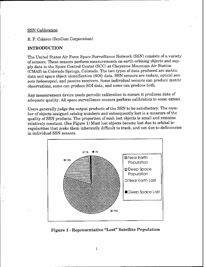
Users generally judge the output products of the SSN to be satisfactory. The number of objects assigned catalog numbers and subsequently lost is a measure of the quality of SSN products. The proportion of such lost objects is small and remains relatively constant. (See Figure 1) Most lost objects become lost due to orbital irregularities that make them inherently difficult to track, and not due to deficiencies in individual SSN sensors.

Dl% "1%

13 Near Earth Population

m Deep Space Population

D Near Earth Lost

■ Deep Space Lost

D79%

Figure 1 - Representative "Lost" Satellite Population

A differential correction (DC) process performed in CMAS combines metric observations from many sensors to produce an element set, or ELSET. (An ELSET is a mathematical description of an orbiting object's motion relative to the earth.) The ELSET is then propagated forward in time to predict the object's position for such purposes as maneuver detection, collision avoidance, and re-acquisition by a space surveillance sensor. There is apparently no significant degradation to the space catalog that can be attributed to poor observation quality. This lack of degradation tends to mask the existence of areas where calibration improvement would be worthwhile. The redundancy inherent in SOI data also tends to mask any problems with the quality of an individual observation from a single sensor.

Today's user operational requirements do not stress the SSN. Future requirements such as debris tracking and growth of the space population, coupled with the possibility of no growth (or perhaps shrinkage) in sensor force structure, may require higher-quality space surveillance. Moreover, potential wartime requirements to produce unusually precise orbits on some satellites over a long period of time would impact the SSN's ability to maintain high-quality orbits on ah satellites.

Improvements in sensor calibration have the potential to increase the quality of individual observations at a relatively low cost. Better individual observations mean that fewer observations of each object are needed to produce an adequate output product. This would increase the cost-effectiveness of the SSN.

A comprehensive sensor calibration system would have the following attributes:

1) Calculation of corrections for atmospheric effects on tracking, and automatic insertion of these corrections into sensor operational software.

2) A capability for a sensor operator to see, in near real-time, how the sensor is performing subsequent to tracking a specific calibration target used as an independent standard.

3) Calculation of metric tracking corrections and automatic insertion of these corrections into sensor operational software.

While we do not necessarily know, in an absolute sense, how good we have to calibrate, we probably are able to calibrate our sensors close to the limits of their designs.

The goals of the study that produced this presentation, as tasked by Air Force Space Command, were: identify calibration issues as raised by the people in the field directly responsible for performing space surveillance; prioritize those needs which are the most critical; evaluate alternative feasible solutions; and recommend a pri- oritized list of solutions.

The first phase of the study consisted of surveying the SSN sensors to determine how they currently perform calibration. The results of this survey were reported. Salient calibration issues were identified. In the second phase of the study, candidate calibration upgrades were studied and evaluated for effectiveness and utility. In the third phase of the study, recommendations were formulated for changes and upgrades to calibration procedures and hardware.

Two major calibration issues were identified through the sensor site survey: the need to find a better way of producing reference orbits currently used for metric calibration; and the need to update the radars' atmospheric calibration methods. Although there are many operational issues affecting optical and passive sensors, there were no calibration issues of purely an optical or passive nature identified in the course of the study.

ATMOSPHERIC CALIBRATION

Atmospheric refraction affects propagation of radio signals (e.g., radar tracking signals, satellite control up-links and down-links, and communications signals) between space objects and the Earth's surface. Refraction of a signal is manifest as a bending and a delay of the signal, and affects range, range rate, and angular measurements. Refraction is worst-case at the horizon, decreasing to a minimum at zenith. Although "refraction" characterizes all atmospheric effects, two distinct atmospheric regimes, the troposphere and the ionosphere, with unique physical characteristics, are involved.

Tropospheric refraction of a radar signal is highly dependent on local weather conditions (atmospheric pressure, temperature, and water vapor content). Tropospheric refraction is almost completely insensitive to the frequency of the signal over the relatively small range of frequencies between UHF and X-band. Typical worst-case tropospheric range errors are of the order of 100 meters close to the horizon.

Ionospheric effects along a signal path are generally modeled as a function of the integrated electron density along the path. This integrated density is expressed in terms of total electron content units (TECU). One TECU is 1016 electrons/square meter. Integrated daytime zenith TEC for a 1000 km orbit typically ranges from about 1017 to 1018 electrons/square meter, depending on whether solar activity is at a minimum or a maximum. Worst case solar daytime TEC can range up to 1020 electrons/square meter for low elevation angles. Errors induced by the ionosphere in UHF radars can range from hundreds of meters at the zenith to many kilometers at low elevation angles. (See Figure 2)

Sensor location is a consideration when studying the need for enhanced ionospheric compensation. So is sensor field of view. For instance, the FPS-85 radar at Eglin AFB operates under a region of fairly mild ionospheric activity. However, the radar looks south into an equatorial region of the ionosphere that severely affects satellite

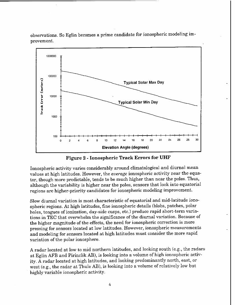
observations. So Eglin becomes a prime candidate for ionospheric modeling improvement.

VI L &

£ L O L L UJ

o L

1000000 T

100000 ::

10000 "

1000 ::

100

Typical Solar Max Day

H 1 1 1 1 1 1 1 1 1 1 1 1 1 1 1 1 1 1 1 1 H

2 4 6 8 10 12 14 16 18 20 22

H 1 1 1 1 1 1 1

24 26 28 30

Elevation Angle (degrees)

Figure 2 - Ionospheric Track Errors for UHF

Ionospheric activity varies considerably around climatological and diurnal mean values at high latitudes. However, the average ionospheric activity near the equator, though more predictable, tends to be much higher than near the poles. Thus, although the variability is higher near the poles, sensors that look into equatorial regions are higher-priority candidates for ionospheric modeling improvement.

Slow diurnal variation is most characteristic of equatorial and mid-latitude ionospheric regions. At high latitudes, fine ionospheric details (blobs, patches, polar holes, tongues of ionization, day-side cusps, etc.) produce rapid short-term variations in TEC that overwhelm the significance of the diurnal variation. Because of the higher magnitude of the effects, the need for ionospheric correction is more pressing for sensors located at low latitudes. However, ionospheric measurements and modeling for sensors located at high latitudes must consider the more rapid variation of the polar ionosphere.

A radar located at low to mid northern latitudes, and looking south (e.g., the radars at Eglin AFB and Pirinclik AB), is looking into a volume of high ionospheric activity. A radar located at high latitudes, and looking predominantly north, east, or west (e.g., the radar at Thule AB), is looking into a volume of relatively low but highly variable ionospheric activity.

UHF radars (i.e., most of the sensors in the SSN) are very sensitive to ionospheric effects. Un-corrected UHF observations regularly exhibit ionosphere-caused range errors of 500 - 700 meters at normal tracking elevations. Near the horizon, total tracking errors (with range and angle components considered) can be many kilometers. The state of the art in ionospheric measurement and modeling can get the high-angle range error down to about 30 meters. This corresponds to about 5 TECU at UHF, which appears to be the lower limit for errors in estimating or modeling electron content with currently employed techniques. A range error of 30 meters is probably acceptable for the SSN, since the differential correction process generally produces an ELSET of "acceptable quality" from several such observations.

Possible ionospheric calibration methods cover a broad spectrum, but share the common attribute of producing an ionospheric map over the site. This map describes the estimated effects of the ionosphere, based on some analysis of the physical phenomena causing the effects, in a form the site's computers can understand. The map must be embedded in the site's operational software in such a way as to be available to apply corrections to observations. The actual structure of the map is dependent on the site configuration.

Methods for modeling and measuring the effects of the ionosphere fall into several broad categories:

1) Empirical models that rely on a few generalized parameters to build an average or representative (time-variant or time-invariant) estimate of ionospheric effects. Empirical models are not generally accurate enough for operational calibration except in benign, predictable environments. They are, however, valuable as backups to other techniques in times of equipment failure, or for use as one component of a more complicated methodology.

2) Observational models that rely on a distributed network of collection points to accumulate data used to build a description of the ionosphere over a region or over the entire Earth. These models represent an improvement over purely empirical models since they use actual measurements of the ionosphere. When combined with an appropriate empirical model, observational models can produce fairly accurate ionospheric maps. The major limitation to these models is that ionospheric measurements are generally not taken at the site of interest, and in some cases are taken no closer than several thousand miles. This introduces errors into ionospheric predictions due to lack of knowledge of actual conditions at the modeled location. It also introduces errors caused by translation of predictions from the collection points to the customer sites.

3) Systems that make ionospheric measurements at the site and construct a map over the site, often in conjunction with an empirical or an observational model. These systems have the advantage of producing ionospheric maps that are accurate and valid for the site location, limited only by timeliness and availability of obser-

vational objects. These systems typically derive ionospheric data from observations of GPS or TRANSIT.

4) Systems that are built into the sensors by design. (This is probably the ideal situation.) For example, PAVE PAWS solid state phased array missile warning and space surveillance radars have a unique internal ability to map the local ionosphere.

AFSPC has proposed a centralized support architecture to supply ionospheric data to missile warning and space surveillance sensors. Data would be collected in the field, and would be quality-controlled at the 50th Weather Squadron (50 WS). The 50 WS would use the data in the current PRISM model, the developmental Iono- spheric Forecast Model (IFM), and future planned models to produce products tailored to individual sensors. These products would then be sent to the sensors as often as required. This approach would probably be adequate for those sensors that do not look into equatorial latitudes. Some of this capability exists today, and the remainder would be phased in over the next few years. The 50 WS supports some sensors today, and its capability can be improved both in scope and quality at low (AFSPC estimate) cost to the SSN.

METRIC CALIBRATION

SSN sensors perform external metric calibration using a variety of satellites. Most sensors rely on TRANSIT satellites, or precision reference orbits on other satellites produced by the MIT/LL Millstone Hill facility. Any replacement methodology must utilize a set of satellites containing both near-Earth and deep-space objects with precision reference orbits readily available.

A worldwide network of internationally-operated laser stations, managed by NASA, gathers satellite observations. These observations are used to determine station positions and other data necessary for the study of the solid Earth. A by-product of these observations is a well-maintained set of precision orbits (to approximately 1 cm accuracy) on a variety of near-Earth and deep-space satellites. These orbits are available through the Crustal Dynamics Data Information System (CDDIS). Also available, and potentially more useful, are quick-look ranging observations on these satellites. Another alternative for metric calibration is the RADCAL satellite (object number 22698). Figure 3 contains a list of candidate reference orbit satellites and some of their orbital parameters.

The data available from NASA's CDDIS should be adequate to generate reference orbits for all sensors. Each sensor could be tasked for observations on all candidate reference satellites that pass through its coverage. Personnel at each sensor could evaluate quality of tracking and determine a priority order of reference satellites for their sensor. The 1 CACS, with assistance from SWC/AE, could develop procedures to produce reference orbits from NASA laser ranging data, using SWC/AE software. The 1 CACS could tailor orbit production to actual satellite passes over individual

sensors, and transmit orbital segments with the same frequency Millstone does today. Sensor metric calibration procedures could remain unchanged.

Satellite Number

Name Period (Minutes)

Inclination (degrees)

Apogee (km)

Perigee (km)

UHFRCS (square meters)

TBD GFZ-1

1328 EXPLORER 27 107.7 41.2 1302 936 3.7042

1726 EXPLORER 29 120.3 59.4 2277 1112 2.9932

3093 EXPLORER 36 112.2 105.8 1574 1082 2.1646

7646 STARLETTE 104.2 49.8 1107 805 0.1557

7734 GEOS3 101.6 115.0 852 817 1.5852

8820 LAGEOS 225.5 109.9 5947 5839 0.0462

10967 SEASAT1 100.1 108.0 767 763 42.7365

16908 EGP 115.7 50.0 1497 1478 3.5226

19749 GLONASS 40 675.7 65.1 19144 19115 4.9179

19751 ETALON 1 675.6 65.1 19156 19095 0.3557

20026 ETALON2 675.4 65.4 19147 19096 0.3228

20619 GLONASS 44 675.7 65.3 19194 19066 0.8868

21006 GLONASS 47 675.7 65.1 19277 18983 1.945

21574 ERS1 100.5 98.6 785 783 27.8037

21853 GLONASS 53 675.7 65.0 19148 19111 2.9867

22056 GLONASS 56 675.7 64.8 19146 19114 3.1446

22076 TOPEX 112.4 66.0 1344 1332 14.957

22195 LAGEOS 2 222.5 52.6 5951 5617 0.1

22779 GPS 34 718.0 54.5 20238 20129 3.8079

22782 METEOR 2-21 104.1 82.6 970 937 16.6337

22824 STELLA 100.9 98.6 805 797 0.1541

22969 METEOR 3 109.4 82.6 1209 1186 9.9573

23027 GPS 36 718.0 55.0 20356 20009 4.9765

23101 MSTI2 92.8 97.1 420 405 0.9867

23560 ERS2 100.5 98.6 785 783 15.9994

Figure 3 - Laser Reference Satellite Orbital Parameters

RECOMMENDATIONS

Following are the recommendations for atmospheric calibration at the respective sensors, in priority order:

1) Maintain the MIT Radar Calibration System (MRCS) at Eglin. MRCS should be the model for an integral, stand-alone, comprehensive, on-site calibration system. Now that development costs are paid, MRCS O&M costs should be included in Eg- lin's budget. Required contractor support, if any, should be studied and specified by Eglin. Explore a real-time feed from the 50 WS Ionospheric Measuring System (IMS), or data products from 50 WS. These would replace the Bent model currently used in MRCS operation, and act as a gap-filler in case of MRCS equipment failure.

2) Replace the TRANSIT-based ionospheric calibration system at Pirinclik with a GPS-based system. Possible candidates are an ionospheric subset of MRCS, the Ionospheric Error Correction Model (IECM) being installed at ALTAIR, and the IMS. Performance of MRCS is well-understood, but it is too early to evaluate performance of IECM. Explore a real-time feed from IMS or data products from 50 WS to augment and back up on-site measurements.

3) Make no immediate changes to PAVE PAWS. Examine 50 WS products to determine if any improvement can be made to the data supplied to PAVE PAWS. (The results of a PAVE PAWS Ionospheric Calibration study performed by MITRE Cor- poration suggest substitution of a real-time ionospheric modeling system for the internal PAVE PAWS ionospheric measurement technique would greatly improve accuracy of range measurements. During the MITRE study, MIT/LL's GPS Real-time Ionospheric Monitoring System (GRIMS) and Phillips Laboratory's Ionospheric Er- ror Correction Model both demonstrated 50-70% reductions in radar range errors.)

4) Replace the monthly ionospheric updates at the Fylingdales radar with a real- time feed from IMS or data products from 50 WS.

5) Replace the time-invariant ionospheric model at the NAVSPACECOM radar with a real-time feed from IMS or data products from 50 WS.

6) Incorporate changes in the Thule radar's software to use external ionospheric data. Supply data through a real-time feed from IMS or data products from 50 WS.

7) Supply a real-time feed from IMS or data products from 50 WS to the radars at Clear and Cavalier. Modify site software to use ionospheric corrections.

The above recommendations are made on the basis of technical merit only. Changes to operational sites can only be fully evaluated in the context of cost and schedule impacts. In order to do this, changes must be formally proposed, and cost and schedule impacts must be formally estimated by the responsible organizations.

FURTHER STUDY

Further study should be done to include the MITRE study results in a follow-on calibration study. This study should include a detailed astrodynamic analysis by SWC/AE. The following questions should be answered:

1) What are the liabilities of relying on off-site measurements for ionospheric calibration?

2) How does the utility of off-site measurements depend on time of day, solar activity, and site location?

3) Is the current implementation of the internal PAVE PAWS ionospheric measurement technique optimum? Can improvements be realized at low cost by opti- mizing the existing technique?

The MITRE study should be used as a model for a similar test of MRCS at Eglin. Although all available data indicate that MRCS produces real improvements in Eg- lin's tracking, no comprehensive test has been conducted with the objective of determining this.

Further study should be done to determine the suitability of AFSPC's proposal of a centralized support architecture for ionospheric data. As this architecture matures, it may achieve the ability to completely replace on-site measurements.

PAGES 11 TO 22 ARE INTENTIONALLY LEFT BLANK.

11

The Midcourse Space Experiment (MSX)

Lt Col B.D. Guilmain (Ballistic Missile Defense Organization) Mr. P.A. Dougherty (Photon Research Associates, Inc.) Mrs. M.C. McLean (Photon Research Associates, Inc.)

Abstract-The Midcourse Space Experiment (MSX) will be the first and only extended duration, multi- wavelength (0.1 to 28mm) phenomenology measurement program funded and managed by Ballistic Missile Defense Organization (BMDO). During its 16 month cryogen lifetime and five year satellite lifetime, MSX will provide high quality target, earth, earthlimb, and celestial multi-wavelength phenomenology data and demonstrate space surveillance and other midcourse sensor functions and key technologies. The data is essential to fill critical gaps in phenomenology and discrimination data bases, furthering development of robust models of representative scenes, and assessing optical discrimination algorithms. The MSX organization is comprised of self-directed work t«mw in six functional areas: hardware, operations, target, target operations, data management, and science teams. These teams provide a unique blend of scientists and engineers from academia and industry. Experiments formulated by each of the eight scientific teams will be executed on the satellite in a 903 km near polar orbit (99.41° inclination), with an eccentricity of 0.001, argument of perigee of 0, and the right ascension of the ascending node is 250.0025. Two dedicated target missions are planned consisting of one Strategic Target System launch out of Barking Sands, Hawaii, and two Low Cost Launch Vehicles launches out of Wallops Island, VA. These target missions will deploy various targets, enabling the MSX principal investigator teams to study key issues such as metric discrimination, deployment phase tracking, cluster tracking, fragment bulk filtering, tumbling re-entry vehicle signatures, etc. A data management infrastructure to ensure that the data is processed, analyzed, and archived will be available at launch time. The raw data and its associated calibration files and software will be archived, providing the customer with a cataloged database containing verified, validated, and carefully calibrated data. This paper describes the MSX program objectives, target missions, data management architecture, and organization.

1. Introduction

There are generic issues for any passive sensor that is required to track and discriminate dim targets against cluttered backgrounds. In the early days of the Strategic Defense Initiative data requirements were identified to address these issues and to fill critical gaps in phenomenology and discrimination databases, validate and enhance models, and improve algorithms.

Based on these requirements a data gathering and measurements system, MSX, was designed, built, and is currently ready for launch. The Midcourse Space Experiment is a multi-year space demonstration and data collection experiment addressing three main objectives for the Ballistic Missile Defense Organization:

- Functionally demonstrate the capability of midwave infrared, longwave infrared, ultraviolet, and visible sensors to acquire, track, and discriminate objects associated with the midcourse (after booster burnout and before reentry) phase of a ballistic missile flight, and of resident space objects.

- Collect a statistically significant natural phenomenology and target signature database to improve and validate models and serve as a system design database.

- Validate key sensor technologies in operational environments over extended periods to support technology transfer. Evaluate extended on-orbit performance data on focal planes, optics, and processors.

In the process of meeting the BMDO objectives MSX will also contribute significantly to the understanding of scientific issues of national interest such as global change, remote sensing, astronomy, astrophysics, and orbital debris.

The MSX "observatory" style satelliteis scheduled to begin its five year mission in early 1996 with a launch on a McDonnell Douglas Delta II booster from Vandenberg Air Force Base, CA.

23

2. Program Overview

The Midcourse Space Experiment will be the first extended duration, multi-wavelength phenomenology measurements program sponsored by BMDO. The MSX program will accomplish its mission by conducting a series of experiments over a period of five years. The period during which the cryogenically cooled infrared sensor will operate is referred to as the cryogen phase (the first 16 months). The remainder of the mission is called the post-cryogen phase.

As experiments are executed, data will be stored on two 54 Gbit recorders. Data will be downloaded via a 25 Mbit per second link to Johns Hopkins University's Applied Physics Laboratory. The Mission Operations Center located at JHU/APL contains the primary Mission Control Center, the MSX Tracking Station, the Mission Processing Center the Attitude Processing Center, and the Operations Planning Center. The Mission Control Center commands, controls, and monitors the satellite's state of health. The Mission Processing Center receives the raw science data and distributes the data to the sensor vendors, and BMDO Data Centers. The Data Centers distribute the data to the MSX Principal Investigators (Pis), and other users. The vendors will verify the data and ensure that their instruments are operating correctly. The Pis will validate and analyze the data from their experiments. The Data Certification and Technology Transfer PI Team will quantify the quality of the data by certifying the calibration and data reduction processes, and specifying data accuracy and precision. All MSX data (science data, calibration records, certified software and final calibration factors) will be archived at the Backgrounds Data Center at the Naval Research Laboratory. The Backgrounds Data Center maintains an on-line catalog to aid in data selection.

3. Satellite

The MSX satellite (Figure 1) structure consists of three main sections: the instrument section, the truss structure, and the electronics section. The satellite structure was designed and built by JHU/APL. The instrument section houses 11 optical sensors, which are precisely aligned so that target activity can be viewed simultaneously by multiple sensors. MSX is capable of observations at a wide range of infrared, visible, and ultraviolet wavelengths. To maintain co-alignment of the sensors, heat pipes are embedded in the aluminum honeycomb panels to keep the temperature even throughout the instrument section. A midsection graphite epoxy truss supports the large cryogenic dewar, which contains frozen hydrogen at approximately 9° K. The 200 cm long truss thermally isolates the heat-sensitive instrument section from the electronic section. Three sides of the truss are covered with multilayer insulation to shield the dewar from the sun and Earth. The attitude control hardware consists of four reaction wheels and three magnetic torque rods. Any three of the four wheels can provide 3-axis control of the spacecraft. Attitude sensors include two 3-axis ring laser gyro systems, a star camera, two horizon sensors, five digital sun angle detectors, and a 3-axis magnetometer. The electronic section carries the warm electronics of all the instruments. Placing the warm electronics in this section minimizes thermal dissipation in the instrument section, allowing the cryogenically cooled instruments to operate as cold as possible. The spacecraft weighs 2800 kg and excluding the two solar arrays measures 510 cm in length with a 150 cm by 150 cm cross section. Raw sensor data is recorded onboard the spacecraft with full fidelity, and later transmitted to the primary ground site over an X-band 25 Mbps downlink. Limited amounts of data may be downlinked in real time over an S-band link at 1 Mbps. Commands are uplinked and satellite housekeeping data downlinked in real time over an S-band link, to either the primary ground site or the Air Force Satellite Control Network. Commands may be executed in near-real time, but are normally stored for execution at a later time. The precise pointing knowledge required by the mission has lead to stringent requirements on the spacecraft for attitude determination, control and stability. The system achieves real-time pointing accuracy of better than 0.1° and post-processing knowledge to 9 microradians. Line-of-sight jitter is held to 9 microradians over instrument integration durations of approximately 1 second. The spacecraft is three-axis stabilized with reaction wheels to provide high precision pointing and maximize sensor performance by not introducing contaminates into the sensor environment. Because there are no expendables on the spacecraft bus (such as propellants), lifetime is limited only by the reliability of the individual subsystems. The spacecraft is powered by a combination of solar panels and a high-capacity, NiH2 battery. This system is

24

designed to deliver 2.5 lew. During data collection events approximately 50% of the available P™« » ™* * the instruments. The primary instrument systems include the SPace InfRared Imaging Telescope (SPIRIT III), Ultraviolet and Visible Imagers and Spectrographic Imagers (UVISR, Space-Based Visible (SBV) instrument, an

On-board Signal and Data Processor (OSDP), and contamination sensors.

SPIRIT ffl a cryogenically cooled infrared sensor, is the most advanced infrared instrument yet launched into space. In the long wavelength SPIRIT m has approximately the same sensitivity but 30 times better spatial resolution than the Infrared Astronomy Satellite.' Developed by the Space Dynamics Laboratory of Utah State University SPIRIT HI includes a five^lor, high-spatial-resolution scanning radiometer and a six-channel, nign- spectral-resolution, fourier-transform interferometer-spectrometer. SPIRIT ffl is the primary sensor for target and background data collection. Its key features include rejection of light from sources outside the field of view and high spatial and spectral resolut.on. The infrared radiometer and interferometer detector bandwidths were'ehosen to address particular data collection needs, including: thermal discrimination, cold target detection,

earthlimb clutter measurement, and atmospheric composition measurement.

UVISI visible Imagers WFOV and NFOV

Ion & neutral mass spectrometers

e.,„H \ Krypton S-oand \ fiashlamp

(telemetry) .. ,.. , antenna MultWayer

insulation blanket-

SPIRIT 3 cryostat

UVISI spectrographic imagers (5)

SPIRIT 3 telescope

UVISI UV Imagers WFOV and NFOV

SBV telescope

Solar Array

ELECTRONICS SECTION - Command & telemetry - RF - Power system - Attitude control - Beacon receiver - Thermal control - OSDP

S-band (telemetry)

antenna

Reference spheres (6)

Optical bench, star camera & gyros

X-band (science) antennas

Figure 1. MSX Satellite

The Ultraviolet and Visible Imagers and Spectrographic Imagers, is a Johns Hopkins University/Applied Physics Laboratory built instrument system with five spectrographic imagers, and four ultraviolet and visible imagers. UVISI provides complete spectral and imaging capabilities from the far ultraviolet through visible wavelengths.

The Space-Based Visible (SBV) instrument, built by MIT/Lincoln Laboratory, will be used to demonstrate space-based space surveillance functions and technology. SBV incorporates a charged^oupled device focal plane a 15^m aperture telescope, a signal processor, and support electronics including an experiment control system telemetry formatter and a data buffer for temporary storage. The signal processor suppresses background clutter, detects moving targets, and generates track reports. It can operate in sidereal track mode,

where it rejects stars and detects moving targets; or in a target track mode, where it rejects the moving background stars. The experiment controller coordinates the operations of each SBV component according to commands received from the ground, and may store a command sequence for later execution. The experiment controller may also be commanded to execute a closed-loop tracking sequence. SBV data can be downlinked m real time at 1 Mbps via the S-band link. The SBV sensor will also supplement the targ^ and background phenomenology data collected by SPIRIT m and UVISI. The spectral coverage of SPIRIT HI, UVISI, and

SBV is illustrated in Figure 2.

The On-board Signal and Data Processor was built by Hughes Aircraft Co. and uses data from SPIRIT HI in real-time signal processing for target detection and tracking. It also will provide information about rad.ation effects on state-of-the-art semiconductor devices.

The contamination sensors, provided by JHU/APL, include five quartz crystal microbalances a pressure sensor, neutral and ion mass spectrometers, and flash lamps to illuminate contaminants in the sensor fields-of-view. These sensors were chosen to measure specific contaminants (such as water vapor) m the spacecraft environment. These measurements will validate the strict contamination control plan followed throughout the development of the satellite, enhance satellite contamination models, and measure contaminants in situ.

S8V

UVISI Imagers Narrow FOV

WidaFOV

HI I I

UVISI Spectrographs

D □

L

1 Q.S 1

Micrometers

r A

SPIRIT III Radiometer

Bin B2Ü CD

SPIRIT III Spectrometer

T-] CD I

CZ3

«StewKft COj Notch

10 IS 20 Micrometers

30

Figure 2. MSX Spectral Coverage

4. Scientific Teams

The Chief Scientist leads the experiment planning function. He interprets the MSX science objectives in light of evolving BMDO and science community requirements. The Chief Scientist also chairs the PI executive committee. This group reviews experiment plans, coordinates with the Mission Planning Team and supporting organizations to execute the experiments, and certifies the analyzed results of the experiments Each PI and his team of experts from various organizations are responsible for defining the science and modeling requirements in their category, designing the experiments, and analyzing the resulting data to satisfy MSX mission objectives and requirements. A brief "mission" objective for each of the eight PI teams follows.

W* Surveillance team's experiments will provide a functional demonstration of the space-based surveillance ^ability, address the detection of space targets against stressing backgrounds, and develop a database of relent ^pace object (RSO) observations. The present ground-based Space *«<^"^£^^ in coveragTcapacity, sensitivity, available optical wavelengths, and accuracy. MSX will be the first space-

26

based platform covering optical wavelengths from ultraviolet through long wave infrared to investigate wide-area

space surveillance.

The Space Surveillance team's catalog maintenance experiments are designed to exploit the greater observing opportunities afforded by a space-based platform to address issues of coverage and capacity. These experiments account for spacecraft constraints, communication limitations, and data accuracy, as well as uncertainties in the existing catalog. Surveillance team experiments will also demonstrate space object identification. There are also three experiments concerning space debris. One will use all MSX sensors to develop a multispectral model of space debris. Multi-spectral data from the MSX instruments will be combined to yield information about the albedo (percent reflectivity) and size of the object. These results will address the existence of radar-transparent debris. A second survey experiment will compile a database of existing debris. The third will capture a satellite breakup, should one occur, and provide detailed data on the resulting debris and its relation to the debris population. The dynamics of the fragmentation can then be studied, yielding information about the cause of the event. Limited measurements of the on-orbit flux of debris onto a given space platform have been made. The SBV can search in preferential locations from which the current model predicts most of the orbital debns will come. Objects seen in specific directions over a given time period will be counted. The data will contribute to the design of specific strategies for early warning of debris collision.

The Earlv Midcourse Target team concentrates on the phenomenology and functions associated with the boost through deployment phase of ballistic missiles. This team will address target acquisition, deployment, and tracking against cluttered backgrounds, as well as metric discrimination. This PI team will use the dedicated target missions as the primary source of data. Targets of opportunity will be used to supplement this data.

The Theater and Midcourse Cooperative Target team will concentrate on the latter phase of a missile's exoatmospheric trajectory and will demonstrate tracking and handover functions on credible targets. This PI team is concerned with payload evolution from post-deployment through reentry. This team will focus on thermal and dynamic discrimination, and target signature collection.

The terrestrial, earthlimb, and celestial backgrounds targets are observed against influence target measurements. PI teams will make dedicated background measurements over a variety of conditions to provide real data to evaluate their impact on sensors and overall system performance. Atmospheric background measurements will be collected as a function of tangent altitude, latitude, season, and atmospheric conditions. The goal is to establish the characteristics of small scale spatial irregularities of earth and earthlimb backgrounds and to determine their global distribution, associations with certain phenomena, and frequencies of occurrence. Experiments will measure and characterize the effect of celestial structures and moving backgrounds, earth radiance, and atmospheric signal attenuation existing at low elevation angles, and also measure photon noise generated by zodiacal background.

The Earthlimb/Aurora team and Shortwavelength Terrestrial Backgrounds fSTB-) team will obtain ultraviolet through very longwave infrared data which is required for evaluation of missile defense system performance against stressing earthlimb and terrestrial backgrounds. Earthlimb experiments will focus measuring earthlimb radiance, auroral emissions intensities, radiance, and structure, and on the spatial distribution and IR radiance of mesospheric clouds and terrestrial clutter. The STB team will focus on characterizing the terrestrial auroral and airglow limb and below-the-horizon spectral databases in the 110 to 900 nm wavelength range. The goal is to acquire a representative database on global, seasonal, diurnal, and temporal variations simultaneously in the ultraviolet through infrared wavelengths.

The Celestial Backgrounds team will characterize representative and stressing celestial backgrounds. The results of the celestial background experiments will upgrade the brightness/resolution databases to satisfy strategic defense system requirements. Celestial background measurements will be providing a comprehensive survey of the stellar sky with emphasis on the solar system structure, detail, and point sources.

The Contamination team has oversight of contamination control and monitoring through the life of the program. They oversee material choice and handling during hardware development and integration, through the

27

contamination control plan. This plan will be validated by on-orbit data and will be a legacy to future satellite programs. The contamination team is responsible for monitoring, modeling and documenting the effects of contamination (from the spacecraft and from the ambient environment) on optical sensors. The contamination experiments quantify contamination effects on optical sensor performance. The contamination team will update pre-launch models developed for use in predicting obscurants, measure in-flight contaminates, and characterize particulate and molecular contamination in the space environment which impair the functioning of space-based sensors and limit their effective lifetime.

The Data Certification and Technology Transfer (DCATT) team oversees the calibration of the sensors, certifies the quality of the data, and transfers the results of the technology demonstrations and lessons learned to other DoD programs. The DCATT team represents a unique approach to sensor characterization. The DCATT team is an integral part of sensor characterization, and as such provides the interface between the Pis and sensor vendors.

Pre-launch, the DCATT team works with each sensor vendor to develop, implement, and document a sensor calibration plan. They also work together to develop and implement in software a set of algorithms to calibrate the raw sensor data (CONVERT), and develop an automated process for verifying the quality of the data (Pipeline). This allows the production of high quality calibrated data in an automated, repeatable fashion. The certification technique used is similar to a method of process certification used in manufacturing.

The DCATT team will use the calibration data (ground and on-orbit) to establish bounds within which the sensor operations is "nominal". Within these bounds, the process by which the raw data is converted to engineering units will be certified by the DCATT team. MSX is a scientific data gathering and measurements program and great care has been taken to understand each instrument and its calibration requirements. Calibration on the ground and on-orbit with reference spheres, stars and internal stimulators are all traceable to National Institute of Standards and Technology standards. The DCATT team will determine the metric and photometric accuracy and precision of the sensors (with error bounds), biases in the metric data and absolute photometric calibration. The DCATT team will also provide traceability to sensor measurements- a means to investigate problems with on-orbit sensor performance. DCATT activities will enable MSX to define actual sensor performance capabilities.

5. Targets

The Targets Teams develops and procures target objects, instrumentation and launch vehicles for the MSX dedicated target experiments. They test and characterize the target objects. They are also responsible for ensuring the targets are ready for launch when required, and conducting launch operations. The U.S. Army Strategic Defense Command executes the Strategic Target System (STARS) mission and directs target development at Sandia National Laboratories for the STARS and Low Cost Launch Vehicle missions. The Air Force's National Aerospace Intelligence Center executes the Low Cost Launch Vehicle program.

The dedicated targets include a number of test objects deployed from the Operational Deployment Experiment Simulator, launched on the Strategic Target System booster. One dedicated target will be launched from the Kauai Test Facility in Kauai, Hawaii, and impact in the broad ocean area north of the US Army Kwajalein Atoll. The Post Boost Vehicle launched on the STARS II booster will deploy twenty-six midcourse objects. These 26 objects represent a number of different target types and deployment techniques. All the target objects will be deployed in sunlight and will subsequently cross the Earth's shadow into darkness. Two Low Cost Launch Vehicles will be launched out of Wallops Island, VA. Each of these sounding rockets will carry at least five highly characterized targets.

These target missions will lead to the development of an extensive database of midcourse target signature phenomenology observed from a space-based platform.

28

6. Operations

MSX satellite operations are carried out by cooperating teams from several organizations. These teams are responsible for scheduling and executing spacecraft activities, collecting the data, and maintaining the health of the spacecraft.

The Mission Planning Team (MPT) consists of the Program Manager, Chief Scientist, Technical Advisor, System Engineer, and representatives from user organizations. The MPT validates and prioritizes the mission requirements and experiment plans, and develops a master plan for performing experiments to satisfy the mission requirements. The Mission Planning Team provides the Operations Planning Team (OPT) with monthly objectives based on the master plan. The OPT analyzes each experiment to ensure it can be accomplished without violating spacecraft constraints, and then schedules the experiments to meet the monthly objectives. Satellite resources required to execute each experiment are estimated by the OPT in close coordination with the Pis and the sensor vendors. This enables the MPT to assess the "cost" versus the benefit of each experiment, and helps ensure the most efficient utilization of the satellite's resources. This planning is vital during the cryogen phase of the mission.

The SBV Payload Operations and Control Center at MIT/LL participates in the planning process for surveillance experiments. The OPT then produces the set of commands needed to run all scheduled spacecraft activities, and hands them off to the control team. The Operations Control Team is responsible for uplinking the commands to the spacecraft, downlinking the recorded data and real time data, and monitoring the spacecraft health and status. Uplinks and downlinks may be directly between the Mission Operations Center and the spacecraft, or they may go through the Air Force Satellite Control Network (recorded data can only be received at the Mission Operations Center, because of the high data rate). The Test Support Center is the secondary ground site, and has the capability of commanding the spacecraft if necessary.

The On-orbit Spacecraft Performance Assessment Team and the sensor performance assessment teams monitor spacecraft and sensor performance, and identify, diagnose, and resolve problems with the spacecraft and sensors.

7. Data Management

The MSX Data Management system has been designed to swiftly flow the data to the end users. Data Management responsibilities extend from telemetry processing through data reduction, and to distributing the data products to the scientist and other users. Data processing tasks are distributed so that experts may do their part at their home institutions. Initial processing is done at the APL Mission Processing Center. Tapes are sent simultaneously to the Data Processing Centers (one for each sensor) and the data archive and distribution centers (BMDO Data Centers). The Data Processing Centers (DPCs) monitor and verify the quality of the data and maintain the calibration software and associated calibration products. Data verification is done using an automated "pipeline" process which is certified by the DCATT PI team. Data certification is done by the DCATT PI Team with participation of the sensor vendors and Pis. Data analysis and validation are done by the Principal Investigator teams. The primary archive and distribution center is the Backgrounds Data Center, at the Naval Research Laboratory. The archive includes pre-launch testing and calibration data, all mission data, data quality indicators from the DPCs, supporting (non-MSX sensor) data, calibration software and associated calibration factors, and all PI analysis products. Due to the volume of data anticipated from this program, a "pipeline" data management architecture has been implemented in which automated tools are used whenever possible to minimize any processing delays. The Data Centers automatically distribute data to the Principal Investigator Teams' Data Analysis Centers. The archive data are available upon request to the broader DOD and science community, with proper clearance and approval from the MSX Program Manager. A top level MSX sensor data flow diagram is presented in Figure 3.

29

MISSON OPERATION CENTER (MPC. APC. OPC)

JOW« KOPW« WAffUED FWSCS LAB

DATA DISTRIBUTION

CENTERS

04CKISSOUMCS DATA CW (POMASY MSX AfiCWVB

MCCOIAE QAIA CIR

FUAC? DAXA cm

MSX SENSOR ANO

SUPPORTING DAEA.

ANOMAUES CAL DATA SUMMARIES*

. PROCESSING CHANGES

CAL UPDATES

SENSOR ENGINEERING TEAMS

OVERSOW

PI DATA ANALYSIS CENTERS DATA

CERTIFICATION PI

TEAM

Figure 3. MSX Sensor Data flow

8. Organization

The MSX program is comprised of self-directed work teams in six broad functional areas: Principal Investigators, spacecraft and ground operations, sensors, targets, and target operations. The MSX program has over 300 individuals from more than 30 organizations. Actual implementation of technical direction was left to the self directed work team with assistance and lessons learned passed on from other teams in the MSX organization. A collective decision making philosophy is exercised in which individuals are involved in decisions which could affect their area of responsibility. Program management has focused on the financial, technical, and schedule constraints bounding each team's environment, and has ensured that all interfaces between organizations are met and controlled.

Managed by the Ballistic Missile Defense Organization and executed by universities, the MSX program has no prime contractor. The principal organizations involved in key program elements are listed below and illustrated in Figure 4.

=sr I ä

Figure 4. MSX Organization

30

p. Summary

The MSX satellite has a suite of state-of-the-art sensors covering the spectrum from the far ultraviolet to the very longwave infrared. It will provide data to answer fundamental questions about the performance of BMDO surveillance systems, and provide environmental data of global interest.

MSX will rriinimize risk in the development of critical National Missile Defense and long-range theater missile defense systems by collecting high-quality data sets on threat-realistic targets against real backgrounds with state-of-the-art sensors; collecting global, seasonal statistics on stressing background clutter against the earth, earthlimb, and celestial backgrounds; and validating key sensor technologies such as focal planes, optics, and processors in operational environments over extended periods to support technology transfer.

MSX will also contribute significantly to the understanding of scientific issues of national interest, such as global change, (ozone chemistry, global warming, earth resources imagery), and basic science (astronomy, astrophysics and orbital debris, solar/terrestrial interactions, and celestial radiometric standards).

The MSX program will provide valuable insight into the operation of a tasked spacecraft, distributed data processing, and the efficient archive and retrieval of very large data sets. The infrastructure for experiment planning, operations, and data reduction and analysis is in place. Spacecraft integration is nearly complete and

launch is planned for early 19%.

10. References

[1] J. Mill, R. O'Neill, S. Price, G. Romick, O. Uy, E. Gaposchkin, G. Light, W. Moore, T. Murdock, A.T. Stair Jr, Midcourse Space Experiment: Introduction to the Spacecraft, Instruments, and Scientific Objectives, Journal of Spacecraft and Rockets, Volume 31, Number 5, September-October 1994.

[2] Richard Huebschman & Tom Pardoe., "The Midcourse Space Experiment Spacecraft," AIAA Paper 92-

0977, Feb 1992.

[3] Midcourse Space Experiment "Program Management Plan," BMDO, Feb 1994.

[4] Midcourse Space Experiment Program, JHU/APL, Jan 1994.

[5] Harry Ames & David Burt, Development of the SPIRIT III Sensor, Proceeding of the SPIE conference on Cryogenic Optical Systems and Instruments VI, The International Society for Optical Engineering, Vol 2227,

April 1994.

[6] D.C. Harrison & J.C. Chow, Space-based visible sensor on the MSX satellite, Proceedings of the SPIE Conference on Surveillance Technologies, Vol 2217, April 1994.

31

NEW MODES FOR DEBRIS DATA COLLECTION AT THE HAYSTACK RADAR

by D. Hall, T. Morgan, T. Sangiolo and R. Sridharan

MIT Lincoln Laboratory, Lexington, MA

1. Introduction

The Haystack radar, one of the sensors of the Lincoln Space Surveillance Com- plex located in Groton/ Tyngsboro, MA, has been a premier contributor of data on man- made debris in earth-bound orbits '"5. In fact, the debris models today, as captured in Ref. 1 and also in the EVOLVE program used by NASA/JSC and AF/PL. reflect significantly the data collected by the Haystack radar in the range of size of 1 cm. to 10 cm. and altitudes between 500 Km. and 1500 Km.

Recently, Lincoln Laboratory received a request from Mr. Kessler and Mr. Stans- bery at NASA/JSC to examine the region around 3000 Km. altitude for debris. Interest in this region was sparked by a few session of debris data collection at JPL's Goldstone radar which seemed to indicate a relatively high density of debris in near-polar orbits. In response, we developed two new modes at the Haystack radar for data collection. The major reason for the new modes was inadequate sensitivity of the old modes for these higher altitudes. This paper describes these new modes, their characteristics and present some initial test results to confirm their proper operation.

2. Haystack Radar and Debris

The Haystack radar collects data on debris - essentially detections in the beam - by using a stare mode. During any given session, lasting typically a few to 24 hours, the radar points in a specific direction and collects data on all the detections in the beam. These are then processed by NASA with appropriate thresholding and Pd to retrieve "rear detections. Cataloged targets act as controls for assessing that the radar was operating in a valid mode. Substantial data have been collected at 90° elevation and fewer hours at 10°, 20° and 80° elevation. The typical altitudes of debris examined in these modes are 300 Km. - 1500 Km. Most of the data extend from 300-1200 Km. with limited amounts of data collected at higher altitudes.

The mode of operation used by the radar for this data collection consists of a pulse length of 1 ms. at a pulse repetition frequency of 80 Hz. The range of altitudes covered by this mode is typically 300 - 1500 Km. with a resolution of 100 Km. The filters used in this mode cover a range-rate uncertainty of ±7.5 Km/s with a range rate resolution of 15 m/s. The radar's sensitivity in this mode can be characterized as a S/N ratio of 58 dB. per pulse on a 0 dBsm. target at a range of 1000 Km. The radar cross-section of a debris of characteristic size 1 cm. is approximately -43 dBsm. at the Haystack operating frequency (10 GHz.) per the NASA model in Fig. 1. Thus at the canonical range of 1000 km. the

33

radar would record a S/N ratio of 15 dB if the debris were at the center of the beam thus detecting the debris with a Pd> 0.95 on a single pulse. Further, a target in circular orbit at 1000 Km. altitude would transit the beam in a maximum of 0.15 sec. thus yielding 16 pulses of detectable backscatter from the debris, all of which can be coherently or non- coherently integrated to enhance the Pd to >0.999. Almost all the data collected so far with the Haystack radar in its debris mode used the 1 ms. pulse.

The mode of operation defined above has been successfully used by the Haystack radar for 4 years of debris data collection. The detection data are collected whenever the S/N ratio in a specific range-doppler gate exceeds a threshold of-5.2 dB/pulse. The low threshold is set so that any target that exceeds a S/N ratio of 11 dB when non-coherently integrated over 16 pulses will be detected.. The data are written to tape. A typical tape

m

CVS

C Q)

0) > TO

if) o

Fig.

0.01 0.1 1

Size / Wavelength

10

1 : A scaling chart for Characteristic Size to radar cross-section (adapted from Ref. 1)

contains detections from approximately 1-2 hours of stare mode data. Extensive analysis by NASA/JSC has yielded an average detection rate of debris of ~6 / hour when the Hay- stack radar stares close to zenith and the full range and doppler extent is examined. The catalog detection rate is less than 0.25 / hour. It must be remembered that the detection rate includes debris as small as 8 mm. at lower ranges. Fig. 2 is derived from Ref. 1 and depicts these averages.

34

1.2 -

o~ 1- ■*-> u

S § °-8 - § € 0.6 - o -Q 0.4 - <D E © = 0.2 - a S J

01

o in oo

o o in

o in CD

o o 00

o in en

o o

o in CM

o o o m ■sr in

Altitude (1cm.)

Fig. 2. Detection Rate at Haystack Radar for Zenith Pointing (bottom curve : detection rate of cataloged objects)

(top curve : total detection rate)

3. High Altitude Debris

The Goldstone radar at JPL conducted a few debris sessions using their X-band bistatic radar early last year. The range gates examined extended from -500 Km to -3500 Km. The detection rate of debris seen was quite significantly higher than at the lower al- titudes5. "Clumps" of detections were seen in the 800 - 1200 Km. altitude band and above -2800 Km. altitude. Based on preliminary data, Mr. Kessler of NASA/JSC inferred that the debris at the higher altitudes were in nearly polar orbits and were of low radar cross- section. Examination of the extant SCC catalog revealed the following facts:

1. There were four USAF launches into -3000 Km. altitude in the early sixties. The launches were:

Primary Pavload SCC# Intl. Designator Inclination (deg.)

Launch Date

FTV 1169 574 63-014A 09 May 63 FTV/ERS-10 622 63-030A 19 Jul 63 OPS 0856 2403 66-077A 19 Aug66 OPS 1920 2481 66-089A 05 Oct 66

The payloads included the MIT LL experiment called Westford dipoles apart from a number of others of military significance. FTV 1169 was the original "Westford Needles" launch. To date, there are 153 cataloged pieces associated with this launch (Jan 93 NAVSPASUR catalog). No debris from the

35

other three launches have been cataloged.

3. There was also a breakup at this altitude of a rocket body whose mission and orbit cannot be identified.

Mr. Kessler requested help from Haystack radar in characterizing the debris population at these altitudes.

4. The New Modes

It was evident that the search of the higher altitudes would stress the detection sensitivity of even the Haystack radar with the conventional 1 ms. pulsed mode of operation. Hence we developed two new modes with the characteristics shown in the table below. For comparison, the conventional 1 ms. mode is also shown.

Pulse Length 2 ms. 5 ms. I ms PRF (Hz.) 80 40 80

Sensitivity* 61 dB 65 dB 58 dB Range Extent 1200-2400 Km. 2300 - 3500 Km. 300 - 1500 Km.

S/N per pulse on 1 cm. target 8dBs 3dB@ 15 dBA

Range resolution 100 Km. 250 Km. 100 Km. Range Rate Extent ± 765 m/s ± 765 m/s ±7.5 Km/s

Range Rate Resolution 6 m / s 3 m / s 15 m/s # of Pulses on Target in Cir-

cular Orbit at Zenith ~20$ ~18@ ~/0A

*S/N ratio on a 0 dBsm target at 1000 Km. sat a range of 1800 Km. @at a range of 3000 Km.

Aat a range of 1000 Km.

The pulse repetition frequency of the 5 ms. mode had to be reduced so that the desired range extent is covered by the unambiguous range of the pulse. Notice that despite the long 5 ms. pulse, the S/N ratio per pulse on a canonical 1 cm. size debris is low. Multi- pulse processing can bring the S/N ratio to a detectable level (e.g., 10 pulse coherent integration would yield a S/N ratio of 13 dB.). However, this mode should be regarded as capable of detecting debris > 2 cm. characteristic size at 3000 Km. altitude. The radar cross-section of a 2 cm. sized debris is —33 dBsm., yielding a S/N ratio of-13 dB/pulse. With careful processing the debris size for detection can be lowered to ~1.5 cm.

5. Test Results

The new modes have been implemented and tested recently at the Haystack radar. Over 50 hours of 5 ms. data and over 50 hours of 2 ms. data have been collected primar-

36

ily to test and validate these modes. The pointing in both cases was either at or close to zenith (90° and 83.5° elevation).

5.1. Filter Characteristics

Detection of small debris requires that the threshold of detection be set carefully such that the probability of false alarm is low. The threshold has to be chosen with adequate modeling of the filter noise characteristics. Figs. 3, 4 and 5 below are the filter characteristics across the doppler band of respectively the 1 ms. mode, the 2 ms. mode and the 5 ms. mode computed in one range gate. Approximately 1 hour of data have been averaged to generate the characteristics. It is evident that the noise characteristic of the 1 ms. mode is significantly different from that of the 2 ms. and the 5 ms. modes. The latter exhibit a "W" shape across the doppler bands of interest with significant correlation across neighboring doppler bands. The 1 ms. mode uses a 1 MHz. analog filter while the new modes use a 120 KHz. filter. The hardware setup for the two new modes is being examined to find the cause of the filter shape and to correct it if possible.

The noise level in the graphs is represented as an equivalent radar cross section. Thus the difference in the mean noise in the three graphs shows the enhancement in detection sensitivity with the new modes.

5.1. Sample Results

Some of the data collected thus far has been examined for threshold crossings or putative debris detections. A few hours of data have been examined in each mode. An example fly-through of a debris target through the beam in the 5 ms. mode is shown in Fig. 6.

6. Summary

A pair of new modes have been developed and tested at Haystack radar for gathering debris detection data in a stare mode. These modes offer enhanced sensitivity which will enable the radar to characterize the debris in the altitude region of 3000 Km. where there seems to be a significant number of cataloged debris from old USAF launches. We expect to utilize these new modes in support of the NASA/JSC debris modeling effort. These modes will also be useful for the detection and tracking of the reference spheres that will be ejected from the pending launch of the MSX spacecraft.

7. Epilog

One of the questions raised by NASA/JSC is whether the Haystack radar could detect the Westford needles from the MIT LL experiment if they still exist in orbit. First a little history.

37

The first launch of the Westford needles package in October 1961 failed to deploy the needles. Extensive analysis7 showed that "clumps" of needles were deployed in a configuration that militated against the release of the individual needles. While it is possible that a number of debris from the launch could be these clumps, adequate imaging and characterization data do not exist to prove the case. Further, whether any extant "clump" of needles would deploy individual needles is unknown.

The second launch of the Westford needles package was in May 1963. The needles were deployed7. Further, extensive preflight and post-flight analysis of the lifetimes of the needles8 showed that they should decay into the atmosphere in ~3 years. Hence, it is highly unlikely that there are individual needles in orbit.

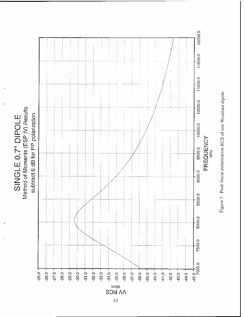
The Westford needles were resonant at the X-band frequency of 8 GHz. which is the frequency of operation of the old Haystack radar and the current Goldstone radar. An individual needle has a peak linear polarization radar cross-section of—35 dBsm. at 8 GHz. The present operating frequency of the Haystack radar is 10 GHz. and the peak radar cross-section of a needle is —45 dBsm.(see Fig. 7) with an average cross-section across all aspect angles of-10 dB. lower. Hence, it is quite unlikely that the present Hay- stack radar with its 5 ms. mode would detect individual needles in transit through the beam even if they exist in orbit.

8. References

I E.G.Stansbery et al: "Haystack Radar Measurements of the Orbital Debris Environ- ment", Tech. Rept. No. JSC - 26655, NASA Johnson Space Center, May 20, 1994.

2. T.E.Tracy et al: "Analysis of Orbital debris Data Collected Using the Haystack Ra- dar", Proc. Of the 1994 Space Surveillance Workshop, Ed: K.P.Schwan, MIT Lincoln Laboratory Project Rept. STK-221, Vol. 1, p. 101, April 1994.

3. S.A.Andrews : "Signature Analysis of Debris Data From the 1994 Air Force Space Command Debris Campaign", Presented at the 1995 AIAA/AAS Space Flight Me- chanics Meeting, Albuquerque, NM, Feb. 1995.

4. S.A.Andrews : "Orbital Debris Radar Calibration Spheres Experiment: Haystack radar stack/Millstone Contribution", Presented at the 1994 Space Control Workshop. USAF Space Command, Colorado Springs, Colorado, October 1994.

5. M.J.Matney et al: "Observations of RORSAT Debris Using the Haystack Radar", Paper presented at the 1995 Space Surveillance Workshop, MIT Lincoln Laboratory, April 1995.

6. R.Goldstein, JPL : personal communication, Oct 95. 7. P.Waldron, D.C.MacLellan and M.C.Crocker : "The Westford Paylaod". Proceedings

of the IEEE, Vol. 52, No. 5, May 1964, pp. 571-576. 8. I.I.Shapiro and H.M.Jones : "Lifetimes of Orbiting Dipoles". Science. Vol. 134, No.

3484. p.973. 6 October 1961.

38

AVG over all pulses for 1 range Gate

-42-

-42.5

Noise RCS

(dBsm)

-43

-43.5

--42

--42.5

--43

--43.5

I 500

doppler bin Index

1000

Figure 3. Filter characteristics of 1 ms pulse.

39

Plot

Y Axis

(Units)

-45.5

50 100 150 x-axis (units)

--45

--45.5


40

AVG over all pulses for 1 range Gate

Noise RCS

(dBsm)

-49.5

100 200 300 doppler bin Index

400 500

49.5


41

Flight Vector and Inclination Angle

0.05-

Elevation Des.

-0.05

Azimuth (Deg.)

Figure 6. Example flythrough.

0.05

- -0.05

42

o o o CM

o Ö - o o

o D.

o T3 o o T3 in o ,_o

C/3 1)

o CJ o c o o o =+- o o 'r_

>- CO Ü U -z. DC

o d o

LU N c

in Ö" C3

LU o LL Cu

o LM

O C3 O 1) o c CD

o o r^- o in <u cu

Ei

o o ON

tusgp

SOd AA 43

An Eglin Fence for the Detection of Low Inclination/High Eccentricity Satellites

W.F. Burnham and R. Sridharan Lincoln Laboratory, Massachusetts Institute of Technology

ABSTRACT

A study was undertaken to design a search fence, using the FPS-85 radar at Eglin Air Force Base, to find low inclination / high eccentricity satellites. These satellites are part of the deep space regime and are difficult to catalog because they do not penetrate the NAVSPASUR fence. Also, most of the sensors in the space surveillance network have difficulty providing efficient search methods for finding satellites within this group.

The FPS-85 is an electronically steered phased array radar that is well suited to both search and track functions. Its location, orientation, and characteristics enable it to provide an effective search strategy for low inclination / high eccentricity satellites.

The study examines a set of possible candidate fence structures, and compares them to a simulation of the current search fence used at Eglin in finding low inclination / high eccentricity satellites. In addition, an analysis is done to see how the various fences perform in finding objects in "typical" catalogs of both deep space and low altitude satellites.

The study concludes that a particular fence design with two segments performs much better than others, including the current SPACETRACK search fence.

1. INTRODUCTION

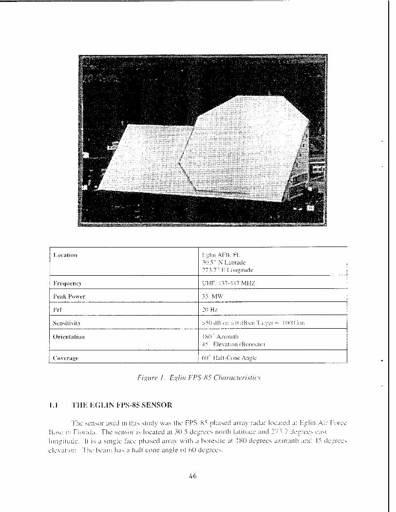
A study was initiated for the United States Air Force Space Command (AFSPC) to design a fence for the detection of low inclination/high eccentricity (LIHE) deep space debris using the FPS-85 phased array radar at Eglin Air Force Base. Figure 1 shows the FPS-85 radar.

The LIHE debris can come from many sources, but one major source is the Ariane-type launches from the European Space Agency facility in French Guiana. Since this launch site is very near the equator (5° N), transfer orbits that take payloads to geosynchronous equatorial positions will have small inclinations. Any failures in these orbits will leave debris in the LIHE

This report examines the effectiveness of the fence currently being used, as well as that of several other potential search fences, in covering debris in low inclination/high eccentricity deep space orbits. In addition, these various fences are also tested to examine their usefulness in covering objects from a typical deep space catalog, and a typical low altitude catalog.

45

Location Eglm AFB. FL 30.5" N Latitude 273.7" E Longitude

Frequency UHF. 437-447 MHZ

Peak Power 35 MW

Prf 20 Hz

Sensitivity >5()dB on a OdBsm Target '" 1000 km

Orientation IN(F A/.imuth 45 : Elevation (Boresite)

Coverage 60° Halt-Cone Angle

Figure 1. Egliu FPS-S5 Characteristics

1.1 THE EGLIN FPS-85 SENSOR

The sensor used m this study was the FPS-Ss phased array radar located at Eel in Air Force Base in Florida. The sensor is located at 30.5 degrees north latitude and 273.7 degrees east longitude. It is a single face phased array with a boresite at 180 degrees azimuth and 45 degrees elevation. The beam has a half cone angle of 60 decrees.

46

The Eglin radar is a primary sensor in the space surveillance network, and can be used for both low altitude and deep space surveillance. Unlike mechanical trackers, the FPS-85 beam is electronically steered, making it an ideal sensor for searching as well as tracking. The various characteristics of the sensor are given in Figure 1.

2. REASON FOR THE STUDY

Low inclination/high eccentricity satellites are difficult to catalog because there are limited sensors available for finding the satellites. Since the inclinations are low, the satellites will not penetrate the NAVSPASUR fence. Similarly, those sensors that have visibility on the objects tend to see them at long ranges since the eccentricity is large and many objects have perigees in the southern hemisphere. Once the targets are cataloged, the network can continue to track the targets, but the initial discovery of the target is a problem.

The Eglin phased array radar is located at 30.5 degrees north latitude and is capable of performing electronically steered searches. The radar is oriented facing due south, so its position and orientation make it useful in the search for the LIHE targets.

Although other sensors, such as those at Kwajalein are capable of tracking the LIHE targets effectively, they are not well suited for the search, or discovery, aspect of the problem.

Since the targets in question may be small in cross-sectional size, the study will examine typical ranges of engagement to determine what targets are expected to be detectable to the radar. Characteristics of the radar, in particular the off-boresite sensitivity, are included in the analysis

3. ASSUMPTIONS

Several assumptions were made in performing the study. First, it was assumed that the pulse repetition frequency (prf) of the Eglin sensor was 20 pulses per second, and that ten of the pulses could be used to perform the search. The remaining ten pulses can be used for tracking and other normal system functions.

The sensitivity of the radar was set at 50 dB on a 0 dBSM target at 1000 km range. Recent tests on the radar showed that its sensitivity actually exceeded this value. Table I shows the maximum detection ranges, at boresite, for various target sizes based on the aforementioned sensitivity.

TABLE 1 Maximum Detection Range vs Target Size

Target size (dBSM) Maximum Detection Range (km)

0 7200

-10 4000

-20 2500

47

The maximum detection ranges shown in Table I are effectively reduced further by an off boresite attenuation proportional to the square of the off boresite angle, (j) i.e. cos2 (j).

4. DATABASE

A database of suitable objects was created by examining the current SCC catalog and selecting all objects with SCC numbers less than 25000 that satisfied the following criteria:

- must have a current epoch - inclination less than 15 degrees (or more than 165 degrees) - eccentricity greater than . 1 - mean motion less than 6.6 revs/day .

Ninety-eight (98) objects satisfied the selection criteria and were included in the database for the low inclination/high eccentricity targets.

5. ENCOUNTER STATISTICS

Using the selected group of targets, the encounter statistics were generated by propagating each of the target element sets for a ten-day period and computing the visibility times for each target at one minute intervals. The STARS program, a computer program developed at Lincoln Laboratory to provide ephemeris information, was used to generate the interaction times. The program outputs the topocentric position and rates of each encounter at specific time step intervals, which in this case was one minute.

Since the program sampled the visibility at one minute intervals, the target positions seldom coincided exactly with the fence line position, and therefore, the intersection points with the fence, and the associated ranges and rates, were determined by linear interpolation of the appropriate positions.

Detectability was determined by examining the range of the target at the point of intersection of the fence. The value of the maximum detectable target range was reduced according to the square of the cosine of the angle between the boresite and the point of intersection on the fence. In order for an object to be considered detectable, its encounter range must be less than the maximum detectable range from Table I, adjusted for angle off boresite.

6. FENCE MODELING

The program allows the user to model the fences as a series of one or two straight lines, or legs. The idea here was to keep the modeling simple, yet provide a realistic representation of various fence styles. Horizontal lines will be lines of constant elevation, and vertical lines will be lines of constant azimuth. Other lines will be chords of a great circle in topocentric space.

48

7. FENCE STYLES

Figure 2 indicates the types of fences used in the study. All the fences are made up of - either a single leg or two single legs. Since the current face of the FPS-85 at Eglin faces due south, all test fence types were centered at a local azimuth of 180 degrees, i.e. looking due south. The extent of each fence determined the number of cells that need to be searched in order to provide leak proof coverage. A beam size of 1 degree was used for the Eglin beam in the analysis.

The current Eglin fence was modeled as an inverted-v type fence. The fence begins at an elevation of 3 degrees at an azimuth of 142 degrees, proceeds to an elevation of 23 degrees at the 180 degrees azimuth position, and returns to an elevation position of 3 degrees at an azimuth of 218 degrees. The actual fence begins at an elevation of about 15 degrees at an azimuth of 142 degrees, peaks at an elevation of 23 degrees at 180 degrees azimuth, and continues to 15 degrees elevation at 218 degrees azimuth. This portion of the fence requires 76 cells for coverage. In addition to this, at both azimuth extremes, "flaps" of non contiguous coverage cells extend to an elevation of 3 degrees. The total coverage requires 100 cells when the "flaps" are included.

The second fence examined was a horizontal fence. The fence was at a constant elevation of 15 degrees, starting at an azimuth of 125 degrees and continuing to an azimuth of 235 degrees. The fence required a total of 110 search cells for complete coverage.

The third fence was a vertical fence starting at an elevation of 3 degrees and proceeding to an elevation of 63 degrees. The fence requires a total of 63 search cells for coverage. This fence continues past the boresite elevation because a 15 degree inclination target can be seen at a 7200 km range at a maximum local elevation of more than 60 degrees.

The fourth fence was an inverted-v (as in the simulated current fence), but here the elevation at the 180 degree position was moved to the boresite elevation of 45 degrees. The fence requires a total of 110 search cells for complete coverage.

The fifth fence was a v-type starting at an elevation of 13 degrees at an azimuth of 120 degrees, dropping to an elevation of 3 degrees at the 180 degree azimuth position, and then rising back up to the 13 degree elevation at an azimuth of 240 degrees. The fence requires a total of 120 cells for complete coverage. This fence extends to the boundary of the 60 degree half cone angle of the full phased array coverage.

The final fence was a cross type, which is a combination of the horizontal and vertical types. The horizontal leg extended from an azimuth of 150 degrees to an azimuth of 210 degrees and was at a constant elevation of 15 degrees. The vertical component extended from 3 degrees to 45 degrees and, again, was located at an azimuth of 180 degrees. The fence requires 100 cells for complete coverage.

49

Simulated

Current

Horizontal

Vertical

Inverted V

V-type

Cross

23

142

15

45

13

3

45

15

3

140

120

150

actual

180

180

180

180

180

218

220

240

210

# Cells

76/100

110

60

110

120

100

Figure 2 . Fences examined.

50

8. RESULTS FOR LIHE OBJECTS

Table II indicates the number of individual unique objects that penetrated each fence, as well as the total number of penetrations. The number of unique objects that entered the fence is fairly even among the fences tested, but the total number of hits is clearly better in the case of the cross type fence. This is because a single pass has the opportunity to enter the fence twice, whereas it can only enter the other type fences once. This is a distinct advantage for the cross type fence over the other types tested.

TABLE II ENCOUNTER STATISTICS (Low-I/HIGH-e TARGETS)

— 98 OBJECTS — 10 DAY RUN

CURRENT

76/100

HORIZONTAL

110

VERTICAL

60

INVERTED-V

110

V

120

CROSS

100 # CELLS

OdBSM

7200 KM

507 534 557 640 676 921 #H1TS

88 85 86 86 86 86 # UNIQUE

-10 dBSM

4000 KM

82 59 110 34 95 165 #HITS

30 32 42 7 36 42 # UNIQUE

-20 dBSM

2500 KM

8 4 9 4 2 13 #HITS

1 1 2 1 1 2 # UNIQUE

An important aspect of the study was to examine each fence and determine if it was leak proof. That is, will an object traveling through the fence always be detected, or can the possibility exist that the beam cannot sample all areas of the fence quickly enough to pick up all penetrations. The STARS program gives information about angular rates as well as the positions, and this information was used to determine if objects could pass through the fence undetected. The maximum angular rate that an object can travel and still be guaranteed to be seen by the fence is given by

max_rate = cell_size * prf / cells_in_fence

where the cell_size here is 1 degree, and the prf available is 10 pulses per second. Table III summarizes the results for the various size targets. The size dependency occurs because of the range restrictions.

51

TABLE III LEAK PROOF TEST

(Low-I/HIGH-e TARGETS) -10 DAY RUN -

CURRENT

76/100 .100

HORIZONTAL

110 .091

VERTICAL

60 .167

INVERTED-V

110 .091

V

120 .083

CROSS

100 .100

# CELLS RATE FOR LP

OdBSM

7200 KM

98 OBJECTS

.250 .256 .261 .222 .262 .261 MAX-RATE

.091 .092 .092 .076 .108 .093 AVE-RATE

N/N N N N N N LP @ MAX

Y/Y Y Y Y N Y LP @ AVE

-lOdBSM

4000 KM

98 OBJECTS

.250 .256 .261 .222 .262 .261 MAX-RATE

.138 .151 .151 .164 .167 .150 AVE-RATE


Y/N N Y N N N LP @ AVE

-20 dBSM

2500 KM

98 OBJECTS

.250 .256 .261 .190 .262 .261 MAX-RATE

.235 .245 .224 .185 .262 .231 AVE-RATE



For the 0 dBSM targets all the fences except the v-type can provide leak proof results when analyzed using the average angular rate at penetration. However, when tested using the maximum angular rates none of the fences will be leak proof.

For the -10 dBSM case only the vertical and the shortened current fence (without the "flaps") will be leak proof at the current rates, and again, none of the fences will be leak proof at the maximum rates.

The -20 dBSM case has no conditions of leak proof status for either the average or maximum rates.

Since none of the fences were leak proof, the number of times that an object passes through the fence becomes more important. If we occasionally miss objects due to prf restrictions, then we would like to have more opportunities to attempt the objects, thereby increasing the probability of detection. Since the cross type fence has a clear advantage in the number of penetrations, it appears to be the best choice for searching for low inclination / high eccentricity targets.

9. RESULTS FOR TYPICAL DEEP SPACE CATALOG

The question now arises as to the effectiveness of the various fences in the tracking of "typical" deep space objects, i.e. those that do not necessarily fall into the LIHE regime. A typical deep space catalog was generated using a subset of objects from the actual deep space catalog. Since the maximum range for detection is 7200 km, no entries were made for circular deep space objects, and therefore, all typical catalog entries here are high eccentricity targets. Figure 3 indicates the breakdown of the typical catalog and the actual catalog.

The typical deep space catalog consisted of 60 objects, and was run against the various fences for a 5-day period. The results are given in Table IV.

TABLE IV ENCOUNTER STATISTICS (DEEP SPACE TARGETS)

CURRENT

76/100 .100

HORIZONTAL

no .091

VERTICAL

60 .167

INVERTED-V

110 .091

V

120 .083

CROSS

100 .100

#CELLS RATE FOR LP

DEEP SPACE 88 106 113 164 113 163 #H1TS

OdBSM

7200 KM

60 OBJECTS

5 DAY RUN

36 36 34 42 34 37 # UNIQUE

.679 .352 1.206 1.331 .646 1.206 MAX-RATE

.141 .118 .196 .213 .130 .172 AVE-RATE


N/N N N N N N LP @ AVE

As in the case of the LIHE targets, the number of unique hits did not vary considerably, but the number of penetrations for the cross type fence was nearly twice that for the current fence. There were no fences that could provide leak proof coverage for either the average angular rate or maximum angular rate at fence penetration. Therefore, the number of penetrations becomes more important. The cross type fence appears to perform better than the current fence in finding typical deep space targets.

10. RESULTS FOR TYPICAL LOW ALTITUDE CATALOG

As a final test, the various fences were tested against a "typical" low altitude database. A typical low altitude catalog was generated using a subset of objects from the actual low altitude catalog. Figure 4 indicates the breakdown of the typical catalog and the actual catalog.

The typical low altitude catalog consisted of 70 objects, and was run against the various fences for a 5 day period. The results are given in Table V.

53

TABLE V ENCOUNTER STATISTICS

(LOW ALTITUDE TARGETS)

CURRENT

76/100 .100

HORIZONTAL

110 .091

VERTICAL

60 .167

INVERTED-V

110 .091

V

120 .083

CROSS

100 .100

# CELLS RATE FOR LP

LOW ALTITUDE

813 805 120 885 861 550 # HITS

OdBSM

7200 KM

70 OBJECTS

5 DAY RUN

70 70 43 70 70 68 «UNIQUE

.276 .283 .574 .501 .339 .447 MAX-RATE

.095 .106 .178 ■ .126 .084 .107 AVE-RATE


Y/Y N N N Y N LP @ AVE

In the low altitude regime, the number of unique hits was clearly poorer in the case of the vertical fence. The targets are moving at high angular rates and stay in the coverage for only a few minutes. There is a large population of high inclination targets in this database, and they can move through the coverage without large changes in azimuth, thus missing the vertical fence. Since the cross type fence also contains a vertical component, its effectiveness was also reduced. The current fence works well in this regime, finding all the targets while also providing a leak proof fence for the average penetration rate. The inverted-v type fence, which is similar to the current fence in shape, but extends up to the boresite elevation, provided a 9% advantage in penetrations over the current fence. This could perhaps warrant an examination of the current low altitude fence to see how it can be improved.

11. SUMMARY

The study looked at the effectiveness of several types of fences in searching for low inclination / high eccentricity satellites. These targets are difficult to find under the current system because they do not penetrate the NAVSPASUR fence. Therefore, cataloging is difficult and serendipitous.

Six fence types were examined in the study, one simulating the current Eglin search fence and five test cases. None of the fences could ensure leak proof coverage when the maximum angular rates at the time of penetration was considered, therefore higher weighting was given to the fence that provided the most penetrations. The cross type fence generated the most penetrations at each detectability range considered, and is the fence type of choice.

A typical deep space catalog was generated and the various fences were also examined under that regime. The cross type fence also performed well in this regime, generating nearly twice as many penetrations as the current fence.

54

Finally, a typical low altitude catalog was generated and the fences were tested in that regime. The current fence performed better than the cross test under this test, and should be retained for low altitude searching. However, the inverted-v type fence provided a 9% advantage over the current fence in the number of penetrations in the low altitude regime, raising the question as to whether the low altitude fence design should be analyzed further.

During the next phase of this project, we will attempt to implement and test the cross fence at the FPS-85 radar.

55

DEBRIS CHARACTERIZATION : AN INTERESTING EXAMPLE by

R.Sridharan, E.M.Gaposchkin, T.G.Moore, L.W.Swezey MIT Lincoln Laboratory, Lexington, MA.

1. Introduction

The Lincoln Space Surveillance Complex located in Massachusetts has been engaged in a number of debris studies " 5| over the last five years. Recently, at the request of NASA/JSC. we undertook the task of detecting and characterizing debris in a specific orbital regime. The objectives of the task were:

1. Detect and track debris that is in the 800 - 1000 km. orbit regime thought to be associated with the nuclear reactor core remnants of a now-defunct Soviet system of satellites '.

2. Assess the characteristics of the detected objects using the L-band and X-band radars and the Firepond optical sensor.

This paper discusses the search strategies that were used at the Millstone Hill radar for these debris. One object was found and quite thoroughly characterized using the Millstone radar, the Haystack radar and the Firepond optical sensor. The results are presented. Lessons learned from this task are also discussed.

2. Sensors at the Lincoln Space Surveillance Complex

MIT Lincoln Laboratory owns and operates several sensors at the LSSC. There are four microwave radars ranging in frequency from UHF (440 MHz.) to Ku-band (16 GHz.). Collocated is the Firepond optical observatory with two visible wavelength optical systems and capability to operate in the infra-red regime also.

The sensors used for this experiment were the Millstone Hill L-band radar, operating at 1295 MHz., the Haystack Long Range Imaging radar, operating at 10 GHz. and the Firepond visible wavelength sensor with the Firepol photo-polarimeter. The characteristics of the radars are shown in Table 1 and those of Firepond in Table 2. All three sensors are networked together such that each can use any of the others as

Table 1 : Characteristics of the Radars

Parameter Millstone Haystack

Operating Frequency 1295 MHz. 10 GHz. Pulse length 1 ms. 256 u.s - 5 ms.

PRF 30-40 1200-40

Antenna size 84 ft. 120 ft. Beamwidth 0.44" 0.05" Sensitivity* 48 dB 52-65

*S/N ratio on a 0 dBsm. target at 1000 Km. range

a designating sensor. The typical mode of operation is to use the Millstone hill radar as the acquisition sensor because of its lager beamwidth. It would then hand off to Haystack which would in turn designate Fire- pond. Each sensor records and processes its own data through existing data reduction algorithms.

57

Parameter Value

Telescope size 1.22 meter F-number f'6.3

Sensor TK 512cb, back-illuminated QE -80%, pixel size 27 u.

Field-of-view data window diam. 30 Jim, search window diam. 300 u.m

Sensitivity 17th Vm with 10 sec. integration 1 deg. Polarization, .02 V,B,R magnitude

Filters U,B,V,R,&I Polarization 1/2 wave plate, Savart plate 2mm separation

3. Search Strategies and Results

This section will discuss the search strategy to find and track the (presumably small) debris that are associated with the remnants of the nuclear power supplies in orbit

3.1. Identification of orbits of interest

The following potential objects were identified (SCC object numbers):

11788, 11971, 12783 13600. 13653 15930 16917, 17035

12319, 12551, 13175, 13594 15085, 15330 15986 18122, 18241

12409,12435 13243, 13416 15378, 15503 16647, 16809 18957,19162

These objects were identified by orbital characteristics and by the label assigned to them by SCC in their catalog. The objects are in pairs because each of these launches left two pieces in high storage orbit. The singletons are cases where only one piece exists in the current catalog associated with the launch. The identification of individual pieces of each pair is uncertain.

3.2. Software Development

A quick assessment of the sensitivity of the search radar (Millstone) and the putative size of the debris objects (< 2 cm.) sought indicated that a new search mode needed to be created for the search. The radar is characterized by a S/N ratio of 48 dB. on a 0 dBsm. target at a range of 1000 Km. The radar cross- section of a 2 cm. diameter sphere at the radar frequency of 1295 MHz. is -43 dBsm. Thus the S/N ratio on a single pulse would be 5 dB at 1000 Km. which is nearly the shortest range for RSOs in orbits of 800 - 1000 Km. altitude. Historically the radar searches along a postulated orbit. However, for the small objects considered here, it was better to search at a relatively low range at an elevation of approximately 45 . i.e.. search along the orbit by staring at approximately the same range and the same elevation in the orbit of an object. The expected S/N ratio on a single pulse is then -2 dB. However, the Millstone hill radar has a beamwidth of 0.44° and hence the debris would dwell approximately 1 second at a maximum in the beam thus permitting a coherent integration of 40 pulses at a maximum. The software modification allowed a •'running" FFT of 32-64 pulses with a resultant expected S/N of 13-16 dB. which is above the detection threshold of the radar. The software was constructed such that the elevation and the number of pulses integrated were under user control. Both the Haystack and the Millstone hill radars modified their software to construct this "time machine" search mode though Haystack, with its much greater sensitivity did not need multi-pulse integration.

58

3.3. Search Results

The Millstone hill radar searched the orbits of ten of the objects of interest using the "time machine" search strategy. The typical search was -25 minutes in orbit. The search was always centered about the parent to ensure that the parent was detected and thus validate the parameters of the search. The search mode was capable of detecting a 2 cm. diameter object in orbit if coherently trackable and approximately a 3.5 cm. size object in orbit were it non-coherent. Based on the earlier Haystack radar detection that drove this search and the deductions by NASA/JSC. the debris would have been expected to be spherical and

hence coherently trackable. No detections resulted.

If there were any slow leaks of debris of the size postulated, the difference in rate of change of the right ascension of the ascending node would have been small(<0.0l deg./day). Hence it can be positively stated that none of the parent objects whose orbits were searched had recently (within 30 days of the

search) leaked/shed any debris of size >2 cm.

4. Serendipitous Discovery

The Lincoln Experimental test Site in Socorro, NM. has been engaged in stare and chase exercises for debris. ETS coincidentally discovered an object in an orbit with an altitude of-950 Km. and with 65 inclination on day 146. The object was reported to be ~ 13th VM (visual magnitude) with no detectable signature. It has been designated as 81215 by SCC. The object is being tracked regularly by Millstone.

The object happens to coincide with 16917 in orbit plane at the present time. Times of coincidence were estimated using the difference in the rate of change of the right ascension of the ascending node and the difference in the orbital period. These estimates are inconsistent with each other. Whether 16917 is indeed the parent is at present unresolvable though it is the closest. There are other sources of debris in these orbital altitudes. For example, there was an old breakup of object 116 (TRANSIT) in approximately this orbital inclination and altitude as well as a Soviet ASAT test.

5. Analysis of 81215

Object 81215 has been tracked by Millstone hill radar, Haystack radar and the Firepond observatory. The metric data from Millstone have been processed through a precision orbit estimator DYNAMO to elicit the drag and radiation pressure effects on the object. The conclusions are as follows:

1. The object exhibits very interesting behavior in its radar signature. Fig. 1 is a typical output of the real-time tracking program SATCIT at Millstone operating at 1295 MHz (23 cm. wavelength). Consistently, the ratio of the radar cross-sections in the orthogonal polarization to the principal polarization throughout the track is - -20 dB. Given the fact that the isolation between the PP and OP channels is of the order of 23 dB. this object has consistently behaved like a sphere at Millstone. Further there have been no detectable periodicities in the signature on a few second time scale. For comparison, Fig. 2 shows a known sphere in track at Mill-

stone.

2. The object, on the other hand behaves like a sphere on some tracks and unlike a sphere on other tracks at the Haystack frequency of 10 GHz. (3 cm. wavelength). Figs. 3 and 4 are examples of the processed radar cross-sections in PP and OP for two different passes. The passes where separated by four days and were taken at similar times, 1700 Z vs. 1800 Z. There is a noticeable periodicity in the signature in Fig. 4 (unlike Fig. 3 ). In Fig 4., the tumble rate appears to change throughout the pass as observed by the changing spacing between the peak responses. The apparent changing tumble rate is caused by the angle between the radar line- of-sight and the object tumble axis changing as the object flies by the radar. There is insufficient data to remove this effect and discern whether the tumble rate is indeed changing. For

59

I"-1- >. wt t 1 " D 1 ! 3 ~ _ _ w > C

O ~ w * D

<• « ^ X X ^ H 5 co

5 - - -

r

o

c ä *• c —

ct

CP 3 JZ

a c

a

6 CO

2 5 a s s 5

or i ■*■ <

i 5 a. a. * X 1 I ■

C o z i. t> »/* >-. c t/» %s% c ■r ■ ■» O w <•» «/I o 1 8 a J3 N O •* X z a T>

§ or

c „ 3 „ w CT> ■ i 4 i r E 1 J 1 „ M » C _J .,_ i ^ E C *

O o 2 o W"l <D Ü 3 f v.

£ £ c • Vj £ *- £ m x. -f a * a u a ^ 6 D ^ o i

o C7* OO ^ O) o a* oo ^ \D */* ., r* Ol _ O O* OD ^ <X> ■ -* < 1 «~l «_* I^J o "^ in :

i 1 1

■ ■—i

I i

< o\ LO ^ n W

I CT\ a fN

y r-H u

i Kj ■^ r. oo n rn en O n CM ■ o u ^ o o \a: rj.

\r~ fX.

a^ CM "1 1 CM

O o

in <%.

LL

A

S

ID

500U

98

-0.3

6

52

64

.3

74

11

.0 0.1

7

6 2-1

/

rm $ CO

? *n ,-( ^H •-<

]

OP

VE

L

0.5

49

8

0

58

36

-90

. 0

U /

■1

8/4

3

j s tj

" -'"■"

$ r "*•" -. o« " 1 o ID

c —

PP

LE

R

475.

6

0.

07

5

0 . 0

99

1

12

/ -2

e i-n

C r* 5 j - 7 O ° ^ {_ _ Q 7 ' r ■w

RA

NG

E

17

5.6

2

2 .

923

0 . 0

02

13

.44.4

9

j _ . r- x ,_« % rv

} fN

1 CM ">

? , m •o- VD CM "^

^ n o o ^ VD - o ,_l

? r- CO *-<

C_^ O o*o

r 04

u

r*--<

U) U o n o ^H o

j *o a: cc

o N w N >° H m < CM O O -i c

CT\ o Cft O CO »~t O ^

en 1 o ^ O

(N WOO ° O 1 *T | CN

o co rx in VD VD m u3 m o

n o v m ^ <n 1—( LTt 00 1 CM t V <N ^ Ü 1 Ü 1 Ü. 1 ' r~ CM ^ r- en *r en ID I > ^ > O \ io 5T n io n n vo (M

< (N rf in a. o M 1 X 1 z X

U W u 0, Q

T- o o

* CM * CM E-"

> o o

3 a. 3 o CD

a v

c o

0)

3

60

c c 3

*H O **i •»

I W -

i cu 7

ä' cS7as

I

i

3BC

o i . « to <N IT) ,J> I—I

iO en (N

* CN

CO O UD C/) a CN (J

^ vo "• <r (N Q "-1

f-H I

Q n CM ^ n ,_, n —I r-t w -1 °

D i-i co o GO ■ • • Cn t—1 TT r-1

8

o N CN

1 <

CN n cn

Cn ^-i co r~* vo •<*

(J <si -« CN

n in

J ° r~ 3 CN ^ >

8

CN

cn o

CD CN O r- O I

I I \o r— vo

cn m o in o r- O CM m

2 O O

TT (N r-t

O

o 1

O T VO CN P- O O -H

O .-! O r-< I O

r- vo vo ,-( in o o ~-t

■ o cn o ■-• o

on

00 ©v

o

01 c o

a) u 3 on

61

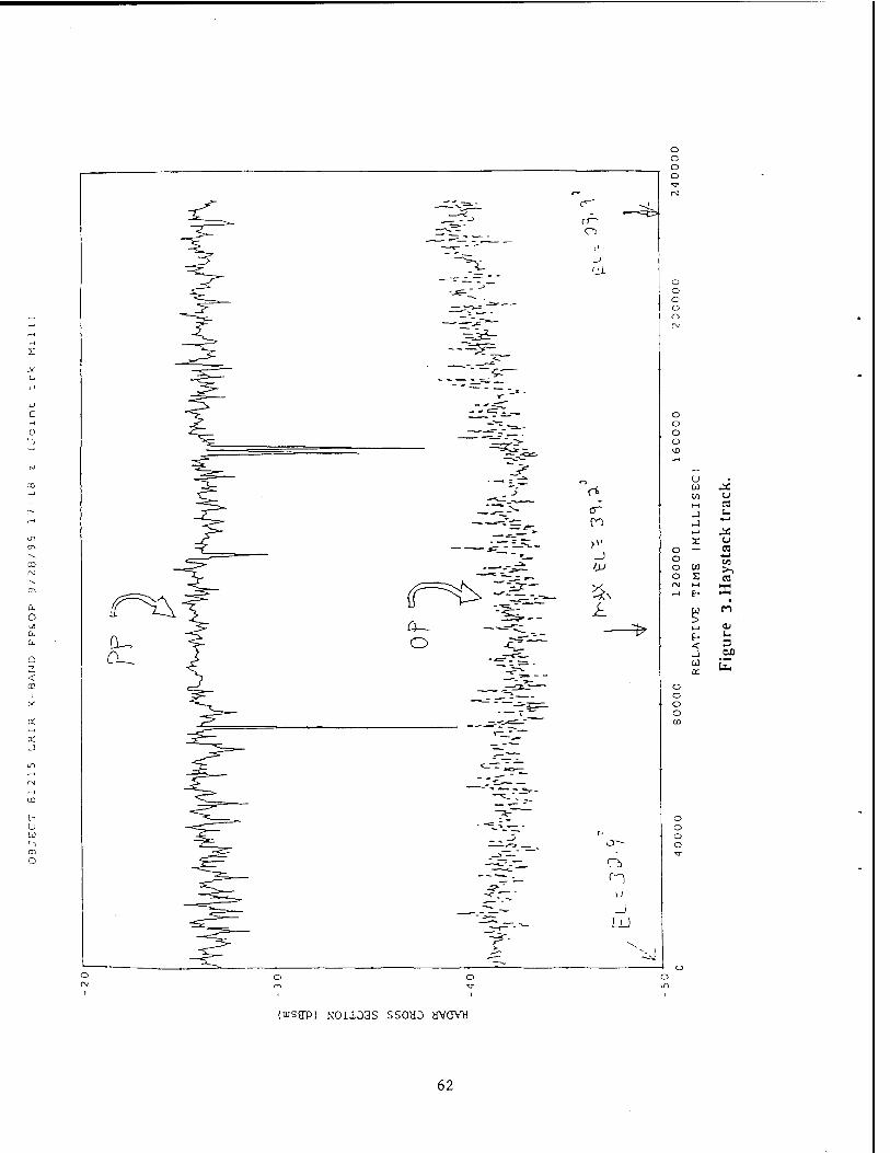
o o

O

o

$r~

Jf

a. O r^

0_ 0_

r^Ä

cr

_)

L ft- o —=&•

f- U ij

-5»-„L_ .

7^-

n

o o o o

o o o o

u w n J J

X o — o o o

u C3 u

03

w i. es E- Ä

% CO

0J

< 3 .) on

fc o o

• o o CD

O o o

(tusfjp) NOixoas SSOMO avovy

62

N

in r-4

00

in

a\

Q

CQ i X

M

u

o

(uisgp) NOIiOHS SSOHD HVOVH

63

comparison, Fig. 5 shows a known sphere track from Haystack. Figure 4 clearly indicates that the object is not a sphere. It is unknown at this time why the object only appears to be tumbling in 24 September 1995 pass.

3. The Firepond data (Fig. 6) show a relatively clean photometric phase curve and low polarization at moderate phase angles both of which seem to argue for a metallic, sphere-like object.

4. The calculated surface reflectivity for 81215 from Firepond data is 0.8-0.87 and the size is -6 cm. in diameter. There does appear to be some brightness variation that would not be present were the object a simple sphere of one material.

5. The mean radar cross-section at Haystack and Millstone are consistent with a "sphere" of ~5 cm. diameter. The photometric and polarimetric data seem to indicate a "sphere" of ~6 cm. All sensors indicate that the surface is metallic.

6. The high quality metric data over a number of tracks from Millstone were used to estimate an area/mass ratio of the object and thereby derive a mass and a density using the size estimates above. Two points are worth noting. The thermosphere model was calibrated by using con- temporaneous data on the well known sphere 5398 in orbit at a similar altitude The resulting density of the object is 1.32± .05 gm./cm3 (see Table 3). Secondly, this analysis assumes that the object is always a solid. Were the object to change phase during the orbit depending on sunlight/shadow and rate of cooling and heating as suggested in Ref. 6. the estimated density would be lower.

Table 3 : Density estimation Orbit Fit Number Standard Error of

Fit Number of obser-

vations M (grams) Density (g/cnr)

1 1.42 403 99.2 1.51 2 1.54 456 95.5 1.45 3 1.30 416 74.3 1.14 4 2.08 458 87.8 1.34 5 1.27 330 70.6 1.07 6 1.69 348 86.7 1.23 7 2.88 832 92.2 1.41 8 1.51 366 82.3 1.26 9 1.63 462 85.6 1.31

6. Summary

An object was found whose size is somewhat large and whose density is anomalously low. The project was successful in demonstrating the techniques for characterization of debris in space using multiple sensors with this object.

6.1. Orbital Information

Detailed orbital information collected on the object that was found. Further, the orbits often cataloged objects that could be potentially leaking have been completely searched thus showing that no recent leakage of objects >2 cm. in characteristic size has occurred.

6.2. Characterization Information

The object found has been characterized extensively with Millstone, Haystack and Firepond. It has been shown to be metallic, with a characteristic size of between 5 and 6.5 cm. Further, its mass and density

64

o o o o Iß

C5

f 1 <f> fll p>->

t/1 M +4 ffi J

t~4 C3

X X. o " <J Ü 03 o 111 1_ o £ *-» (N M 01 -1 k-

01 LC J= .> a H C/j < • J in 0) o>

o 3 o CD o o U,

(USEP) HOI103S SSOtiD HYOYtf

65

"10d%

>

h- LU r> cr < _i ID

o in

Q_ 5 o q

f- o

o CO

X I— O

CL QJ -) m

Q O

j

Z i

O i

Q_ 1

LLI DC

LL

o a s? •a

LU

Ü <3 •o c o z

< a. UJ u C/) < fa I . a

<u u 3 OX)

fa

n TO

t !AI

66

have been estimated. It is slightly denser than water with a density of 1.3 gm/cm if the object is assumed to be solid. In addition, the object has been shown to appear sphere-like at L-band frequency but somewhat un-sphere-like at X-band with a detectable signature. No conclusion has been drawn about the shape of the object.

7. References

1. E.G.Stansbery er al: "Haystack Radar Measurements of the Orbital Debris Environment". Tech. Rept. No. JSC - 26655, NASA Johnson Space Center, May 20, 1994.

2. T.E.Tracy er al: "Analysis of Orbital debris Data Collected Using the Haystack Radar". Proc. Of the 1994 Space Surveillance Workshop. Ed: K.P.Schwan, MIT Lincoln Laboratory Project Rept. STK- 221, April 1994. Vot i P% tc(

3. R. Sridharan : "Characteristics of Debris and Implications for Detection and Tracking", To be pre sented at the 1996 AIAA/AAS Space Flight .Mechanics Meeting, Austin. Texas, 12-15 February 1996.

4. S.A.Andrews : "Signature Analysis of Debris Data From the 1994 Air Force Space Command Debris Campaign", Presented at the 1995 AIAA/AAS Space Flight Mechanics Meeting, Albuquerque, NM, Feb. 1995.

5. S.A.Andrews : "Orbital Debris Radar Calibration Spheres Experiment: Haystack/Millstone Contribu- tion", Presented at the 1994 Space Control Workshop, USAF Space Command, Colorado Springs, Colorado. October 1994.

6. M.J.Matney et al: "Observations of RORSAT Debris Using the Haystack Radar". Paper presented at the 1995 Space Surveillance Workshop, MIT Lincoln Laboratory. April 1995.

67

The Application of the Ionospheric Electron Content Model at ALT AIR

S.M. Hunt(,), G.H. Millman(2), R.E. Daniell(3), L.D. Brown(3), J.T. Lamicela(2), D.L. Sponseller^

INTRODUCTION

The ARPA Long Range tracking and Instrumentation Radar (ALTAIR), at Kwajalein Missile Range, collects positional observations to maintain the satellite catalog for US Space Command on a daily basis. Due to ALTAIR's equatorial location and its UHF/VHF operating frequencies, ionospheric propagation errors can be large and degrade the measurements if not modeled accurately. In 1993 the second phase of a Small Business Innovative Research project was awarded to Research Associates of Syracuse (RAS) and Computational Physics Inc. (CPI was subcontracted by RAS) to create an improved ionospheric model for propagation error correction which would be a significant improvement over the model currently in use at ALTAIR.* These two organizations combined to develop an accurate, low maintenance, Ionospheric Electron Content Model (IECM) to reduce the elevation angle and range errors incurred in near-earth and deep- space satellite tracking. The primary goal of this effort is to furnish a robust system that provides a consistent improvement in the quality of ALTAIR measurements for US Space Command.

The implementation of IECM involved of three main initiatives: 1) developing the base climatological model which is based on the global model, PRISM; 2) implementing the stratified layer method to model the refractive effect of the troposphere and ionosphere at ALTAIR's operating frequencies; and 3) providing accurate total electron content (TEC) measurements, utilizing simultaneous two-frequency (UHF/VHF) ALTAIR tracks or Global Positioning System (GPS) differential delay measurements. Each of these components is described with examples of measured data. A brief overview of the architectural and operational aspects of the IECM implementation at ALTAIR are covered.

1.) MIT Lincoln Laboratory, Kwajalein Missile Range, Kwajalein Atoll, The Republic of the Marshall Islands.

2.) Research Associates of Syracuse, Inc., Syracuse NY. 3.) Computational Physics, Inc., Waltham MA. 4.) Raytheon Range Systems Engineering, Kwajalein Missile Range, Kwajalein

Atoll, The Republic of the Marshall Islands.

ob

EECM OVERVIEW

The IECM consists of two main components; (1) the Ionospheric Correction Algorithm (ICA) which is called by the ALTAIR real-time tracking programs and (2) the Parameterized Electron Content Model (PECM), which creates range and elevation error correction tables for use by ICA. The IECM provides a fully automated ionospheric correction capability that supports real-time dual-frequency (UHF/VHF) and single frequency (UHF or VHF) tracking. Figure 1 illustrates the architecture of the new ionospheric model with the ALTAIR real-time tracking programs.

MEAN SOLAR FLUX DATA

Figure 1. IECM and the ALTAIR tracking programs.

The PECM consists of two parts. The first is the climatological model, and the second is the update algorithm that scales the climatological model on the basis of real-time GPS TEC, ionosonde, incoherent scatter radar and ALTAIR UHF/VHF dual-frequency measurements. Presently, GPS TEC and ALTAIR UHF/VHF dual-frequency

70

measurements are the two real-time sources of ionospheric data available to PECM. Since TEC is proportional to the differential range delay measured by the radar while in dual- frequency UHF/VHF track, the range measurements are used as an ionospheric update by PECM. F10.7cm solar flux data, supplied to ALTAIR by the Air Weather Service, is input for use by PECM on a daily basis.

Included in PECM are mean tropospheric range and elevation error tables created at Kwajalein. Ray tracing is performed through the troposphere and ionosphere (as characterized by PECM) resulting in a range, azimuth and elevation error grid or Ionospheric Specification file (IS file) that is provided to the tracking programs. PECM executes "continuously" (at 15 minute intervals) on its Silicon Graphics Indy (SGI) work station creating one IS file per run. This IS file is written directly to a disk shared by the tracking computer over a local area network (ethernet). A process on the tracking computer orchestrates the maintenance of the IS files for use by the ICA (which is called by tracking programs). A running 24 hour block of these IS files are maintained continuously on the tracking computer disk.

The ICA is used to provide ionospheric range and elevation corrections when called by the real-time tracking programs. The tracking program provides the range, azimuth, elevation, frequency(s) and the desired correction mode to ICA. ICA responds with an apparent-to-true or true-to-apparent range and elevation correction. It interpolates on the most recent IS file providing ionospheric corrections under a variety of circumstances experienced at ALTAIR. Only the obvious situations are mentioned here. ICA is capable of supporting single-frequency or real-time dual-frequency ionospheric error correction at UHF and VHF. The ALTAIR deep-space and New Foreign Launch tracking programs call ICA for single frequency corrections. The near-earth tracking program requests either single or real-time dual-frequency corrections.

The Live-Track data manager is used to pass ALTAIR range measurements to PECM after a dual-frequency track has been executed. PECM uses these data to calculate TEC for an ionospheric update when the next IS file is created. These TEC measurements are used by PECM in a manner consistent with the TEC data obtained from the GPS receiver.

71

REAL-TIME GPS DATA PROCESSING

The Allen Osborne Mini-Rogue GPS receiver provides the capability to continuously update the IECM climatological model output. The receiver calculates TEC using its differential group and phase delay measurements obtained while tracking GPS satellites at 1575.4 MHz and 1227.6 MHz. Differential phase and group TEC data were combined to provide the best possible estimates of TEC for each GPS satellite track. This was done to compensate for large fluctuations in the TEC calculated from the differential group time delay. The differential phase TEC is not as strongly affected by multipath or low signal to noise ratio (SNR). Figure 2 illustrates the information which is provided by the GPS receiver and used to generate the best estimate of TEC for PECM. These data include elevation (deg), differential group delay TEC (denoted as TECg, electrons/m2), differential phase delay TEC (denoted as TECP, 1016 electrons/m2) and SNR. The effects of anti- spoofing (GPS signal encryption) have significantly degraded the quality of TEC measurements obtained from this receiver. To compensate, a new Y-code (crypto capable) Allen Osborne GPS receiver has been purchased for ALTAIR but has not yet been installed.

400

-100 277.15 277.20 277.25 277.30 277.35 277.40

TIME (fractional days, GMT)

Figure 2. Summary of GPS data processed for PECM updates.

The following methodology was used to provide the best estimate of TEC using these GPS receiver data. Data obtained below 35 degrees was not usable due to low SNR. The difference between a weighted (by SNR) seven minute average of TECg (plus bias) and TECp is calculated on satellites above 35 degrees elevation. The difference of the weighted averages is then added to TECP and the resulting value provided to PECM until

72

track is terminated on a particular GPS satellite. Figure 3 illustrates an example of TEC data provided to PECM after being processed in this manner. Occasionally the phase reference of TECP is lost when the receiver momentarily loses track. When this occurs TECp is reset to a new differential group delay weighted average.

-40

WEIGHTED AVERAGE DIFFERENTIAL GROUP TEC

WEIGHTED AVERAGE DIFFERENTIAL PHASE TEC

277.22 277.26 277.30

TIME (fractional day, GMT)

Figure 3. Combined differential group and phase TEC.

Differential group delay bias estimates generated at the Jet Propulsion Laboratory (JPL) are applied to the TEC measurements.1-2 The source of this differential bias is unknown but has been characterized at JPL. The magnitude of these biases are large enough that they cannot be ignored (-.5 to 5 ns). A 5 ns differential bias equates to approximately 30 meters error at UHF and 220 meters at VHF.

73

INTEGRATION AND TESTING AT ALTAIR

The IECM was delivered to ALTAIR on September 25, 1995 and the following is an overview of the results obtained during initial testing.

The IECM was successfully exercised in stand alone configuration (Figure 4). GPS receiver TEC measurements were automatically supplied to and processed on the SGI and then made available to the PECM as a real-time update for IS file generation.

GTS RECOVER SCI(INDY)

NtAMtUKKL

SHARED

TOTAL ELECTRON CONTENT

PECM

TRACKING COMPUTER

DISK

IS FILE MANAGER

IONOSPHERIC CORRECTION ALGORITHM

TEST

PROGRAM

k i

MEAN SOLAR FLUX FIOJ

TESTICA

Figure 4. Illustration of the stand alone configuration.

PECM then wrote the resulting IS files to the tracking computer shared disk area where they were maintained for use by ICA. Test programs which called ICA were used to establish that the system was supplying reasonable range and elevation error corrections. The tropospheric corrections provided by ICA were nearly identical to the existing ALTAIR troposheric correction tables.

Figure 5 illustrates a comparison of ICA TEC calculated with and without the benefit of real-time GPS TEC data. ALTAIR UHF/VHF dual-frequency measurements and the

74

deep-space model values, applied during normal tracking operations for the same period, are also illustrated.

40

30

20

10

UHF/VHF NEAR-EARTH DUAL-FREQUENCY MEASUREMENTS

DEEP-SPACE IONOSPHERIC MCDEL'CORRECTION VALUES

~]

i *

10 20 30 40

0'

TIME (hours, GMT)

Figure 5. Comparison of vertical TEC values from near-earth dual-frequency measurements, operational deep-space ionospheric model, IECM with and without GPS TEC updates. The lapse in the data from hours 18-28 on the upper graph is due to a scheduled maintenance period between tracking sessions at AL TAIR. After its integration with the tracking programs, IECM will replace the ALT AIR operational ionospheric models depicted in the upper graph.

75

The ICA TEC values were calculated at a range of 2000 km, elevation of 90.0 degrees. The ALTAIR UHF/VHF dual-frequency measurements were obtained on satellites above 46.0 degrees elevation at altitudes ranging from 800 to 2000 km altitude. The ALTAIR near-earth ionospheric model treats measured values obtained above 46.0 degrees as if they were made at 90.0 degrees elevation. The deep-space values were those used during two operational satellite tracking sessions. The deep-space model was updated (scaled) with an ionospheric measurement (ALTAIR UHF/VHF dual-frequency) made near 00:00 GMT on each respective day. This comparison provided a first measure to determine whether ICA was providing reasonable ionospheric error estimates when compared to

those already in use at ALTAIR.

TRACKING PROGRAM INTEGRATION

The integration of the IECM with the ALTAIR operational tracking programs is in progress and was initiated due to the good results IECM provided during the stand-alone tests. This section will illustrate how IECM is being tested with the tracking programs and present a snapshot of data collected while tracking near-earth and deep-space calibration satellites. A full statistical summary on the performance of IECM will hopefully be completed for the workshop presentation.

The best measure of truth available to ALTAIR for the deep-space observation metric quality analysis is the DYNAMO reference orbits routinely provided by Group 91 at MIT Lincoln Laboratory. These reference orbits are being used to quantify the improvement provided by IECM. Since the near-earth tracking program at ALTAIR measures the ionospheric error directly, it is being used as the principal truth reference for near-earth metric comparison while being simultaneously compared to a near-earth DYNAMO reference orbit. Table 1 illustrates the different references that IECM is being compared to.

TABLE 1.

TRUTH CATEGORY QUANTITY ALTITUDE SATELLITE AND ALTITUDE (km)

ALTAIR Dual- Frequency track

Near-Earth Only

RvRu (TEC) 90-5000 LCS 4 -800 EGP -1500

DYNAMO Calibration Orbits

Near-Earth &

Deep-Space

Range Elevation

20000 LCS 4 EGP Lageos -5000

76

GPS Reference Orbits

Deep-Space only

Range Elevation

20000 GPS -19000

OTHER KREMS RADARS

Near-Earth Only

Range 90-1500 LCS4

Simultaneous ionospheric corrections are collected using EECM and current ALTAIR ionospheric models while tracking near-earth and deep-space satellites. These data are collected with the UHF/VHF dual-frequency near-earth and single frequency UHF deep- space tracking systems. These tracks take place throughout periods of different daily solar activity. ALTAIR experiences maximum ionospheric propagation error near 2:00 PM and minimum approximately 12 hours later. The maximum rate of change in the ionosphere occurs near 6:00 AM and 8:00 PM as the sun rises and sets. Figure 6 is a comparison of ALTAIR dual-frequency range error measurements to the range errors predicted by EECM with the benefit of an update with GPS TEC data. This track was obtained on EGP (SCC No. 16908) near 9 AM local Kwajalein time and indicates good agreement with IECM. Figure 7 contains ionospheric range errors generated on Lageos 1 (SCC No. 8820) near 8 PM local Kwajalein time with EECM and the ALTAIR deep- space model. The ALTAIR deep-space model and EECM range corrections are in good agreement.

800

600

400

200 UHF/VHF UHF RANGE ERROR MEASUREMENTS

Cm

21.75 21.80 21.85 21.90

TIME (hourS.GMT)

Figure 6. Comparison of ALTAIR dual-frequency ionospheric range error measurements to those simultaneously output by IECM. IECM was updated with GPS TEC data.

11

DEEP-SPACE MODEL

IECMWITH GPS UPDATE

^îî^^nrf-J 55 ■>aliH^B^Hlia^>"^"^M'»î^Mi^"î^^^^"^«MhnrfNyb^^te^h^MdMj

7.70 7.75 . 7.80 7.85 7.90 7.95

TME (hours, GMT)

Figure 7. Comparison of ALT AIR deep-space model ionospheric range errors to those simultaneously output by IECM. IECM was updated with GPS TEC data.

DISCUSSION

Initial results indicate IECM can provide an improved and automated ionospheric propagation error model at ALTAIR with the benefit of real-time GPS TEC data. The continued demonstration of the IECM will provide further information to quantify its improvement to ALTAIR's metric quality. CPU loading measurements and the duration of continuous operation indicate that IECM is robust enough to be integrated with the ALTAIR operational real-time program to provide a consistent improvement in ALTAIR metric quality. Since solar activity is now at a low in its long term (11 year) cyclic behavior, the improvement provided by IECM will be most likely be amplified as its activity increases beginning in 1997-1998.3

Acknowledgments: Art Leivis, Tom Melia, Roberta Gibson, Lincoln Brown (of Computational Physics) and Jeff Lamicela (RAS) executed preliminary testing and configuration of the IECM prior to delivery to ALTAIR. Jeff Lamicela's two week working visit was instrumental to the smooth integration of the IECM at ALTAIR. Loh Thornton of Group 91 at MIT Lincoln Laboratory continues to provide the DYNAMO reference orbits essential to the testing of IECM.

78

REFERENCES

1.) Kieth Stark, Jet Propulsion Laboratory, Private Communication, October 1995.

2.) Lorraine Thornton, Group 91, MIT Lincoln Laboratory, Private Communication, October 1995.

3.) Preliminary Report and Forecast of Solar Geophysical Data, US Dept. of Commerce NOAA, August 8 1995, plO

79

Recent Upgrades at the ALTAIR Radar for Improved Space Surveillance Support

A. Gerber, G. Hogan, MIT Lincoln Laboratory M. Corbin, J. Corrado, J. Mathwig, H. Fitzpatrick S. Murphy, M. Schlueter, J.B. Sherrill, T. White/Raytheon Range Systems Engineering ALTAIR Radar, Kwajalein Missile Range

Introduction

The ALTAIR Radar, located at the Kwajalein Missile Range (KMR) in the Marshall Islands, is one of the prime contributors to the Space Surveillance Network, supplying tracking data on new foreign launches, domestic and cooperative launches, and resident deep-space satellites. A summary of improvements at ALTAIR for space surveillance was last presented at this Workshop in 1994 (Reference 1). Since that time, a number of upgrades have been made, or are in the process of being made, to further improve the space surveillance capabilities of the radar. These upgrades include:

1. Installation of a set of high-resolution waveforms which allow the resolution, discrimination and tracking of closely-spaced objects in deep space;

2. An upgrade to the antenna cable-wrap system which is providing improved capability for the coverage of new foreign launches;

3. Completion of a Star Array Processor signal path upgrade which consolidates near-Earth and deep space tracking operations onto a single signal path;

4. An upgrade of the communications processor used to transmit message traffic to and from Space Command;

5. A GPS-based ionospheric modeling system used to correct for distortions in metric data caused by the ionosphere; and

6. A dual-polarization capability which will allow a complete characterization of the scattering properties of targets at the VHF frequency.

The first four of the these topics will be discussed in this paper; the last two upgrades will be presented in other papers in these proceedings.

High-Resolution Deep Space Waveforms

A new set of waveforms has been installed at ALTAIR to allow the resolution, tracking and discrimination of closely-spaced objects in deep space. These new waveforms are currently being used for two distinct types of activities. The first use occurs while tracking the injection of a new launch complex into a transfer or final deep space orbit. In such cases, the launch complex may include a rocket body and one or more payloads, with some objects spaced by a kilometer or less. Space Command has placed a high

81

priority on being able to resolve, discriminate and track each individual object in the complex at the earliest possible opportunity. The new waveforms are now allowing ALTAIR to provide such coverage. The second use of the new waveforms is for nightly tracks of the resident geosynchronous satellite clusters, in which objects are frequently spaced by less than a kilometer.

Until recently, ALTAIR's deep space waveform suite consisted of a 50 KHz bandwidth search waveform (U1000) and a 250 KHz tracking waveform (U400). The recently installed Universal Signal Processor (USP) pulse compression system has allowed much greater flexibility in terms of waveform design and implementation. A new set of waveforms has been implemented to take full advantage of these capabilities. The new waveforms for use in deep space consist of a 250 KHz U1000X waveform, a 1 MHz U1000S waveform and a 4 MHz U400W waveform, all for use in track mode. The old U1000 and U400 waveforms have also been retained. The properties of the new and old waveforms are listed in Table 1.

Waveform I Length (usec)

BW (MHz)

Max PRF (Hz)

Resolution (m)

I Use

U1000 1000 0.05 50 3000 Search |U400 400 0.25 120 600 Track, Low Res. IU1000X* 1000 0.25 50 600 Track, Low Res. IU1000S* 1000 1 50 150 Track, Med. Res. IU400W* 400 4 120 37.5 Track, High Res. *New Wavefc )rm.

Table 1. ALTAIR Deep-Space Waveforms

The new U400W waveform is the highest-bandwidth deep space waveform, with a chirp bandwidth of 4 MHz. This increased bandwidth provides a range resolution of 37.5 meters, which represents a 16-fold improvement over the capability with the old U400 waveform. The new U1000S waveform combines a 1 MHz bandwidth with a 1000 usec pulse. The additional signal strength gained from a single long pulse, as opposed to several shorter pulses summed with imperfect relative phase coherence, provides an increase in sensitivity for deep space tracking. The new U1000X waveform has the same 250 KHz chirp bandwidth as the old U400 waveform, but has the longer pulse length for improved sensitivity. It should be noted that waveforms up to 18 MHz bandwidth can be created, and are currently in use for near-Earth tracking; however such high resolution has not yet been deemed necessary for tracking in deep space.

The new waveforms received their first operational use during the launch of the GOMS- 0 geosynchronous weather satellite from the CIS on 31 October, 1994 (Figure 1) The launch complex was detected and tracked as an NFL on rev 0, and then again in deep space during its burn into final orbit. Following the burn, the payload was seen slowly separating from the rocket body, but the individual objects were too closely spaced to be tracked in the U400 waveform. Attempts to track in U400 resulted in alternating returns from the two objects, which induced spurious range rates which drove the

82

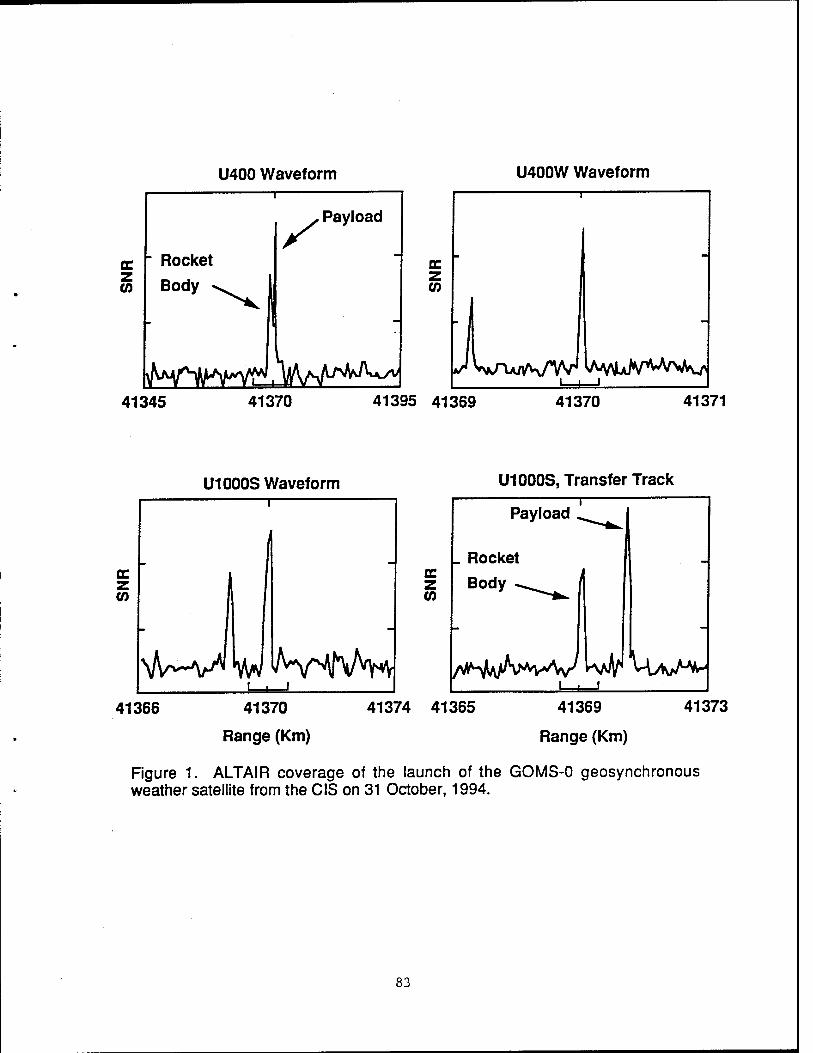
U400 Waveform U400W Waveform

c z CO

41345 41370 41395 41369 41370 41371

U1000S Waveform

DC .

Z 1 CO

\^~v"' I ^ I

41366

U1000S, Transfer Track

DC z CO

41370

Range (Km)

41374 41365 41369

Range (Km)

41373

Figure 1. ALTAIR coverage of the launch of the GOMS-0 geosynchronous weather satellite from the CIS on 31 October, 1994.

U400 Waveform

Jtocket Body

DC Payload 1

Z CO Payload 2

•-W *KA-Ar*l

I Payload 3

U400W Waveform

z CO

23356 23381 23406 23605 23606 23607

U1000S Waveform U1000S, Transfer Track

Payload 3

z CO

rJ vVvMv^ 23770 23774

Range (Km) 23778 24090 23094

Range (Km)

24098

Figure 2. ALTAIR coverage of the launch of three Glonass navigation satellites from the CIS on 20 November, 1994.

84

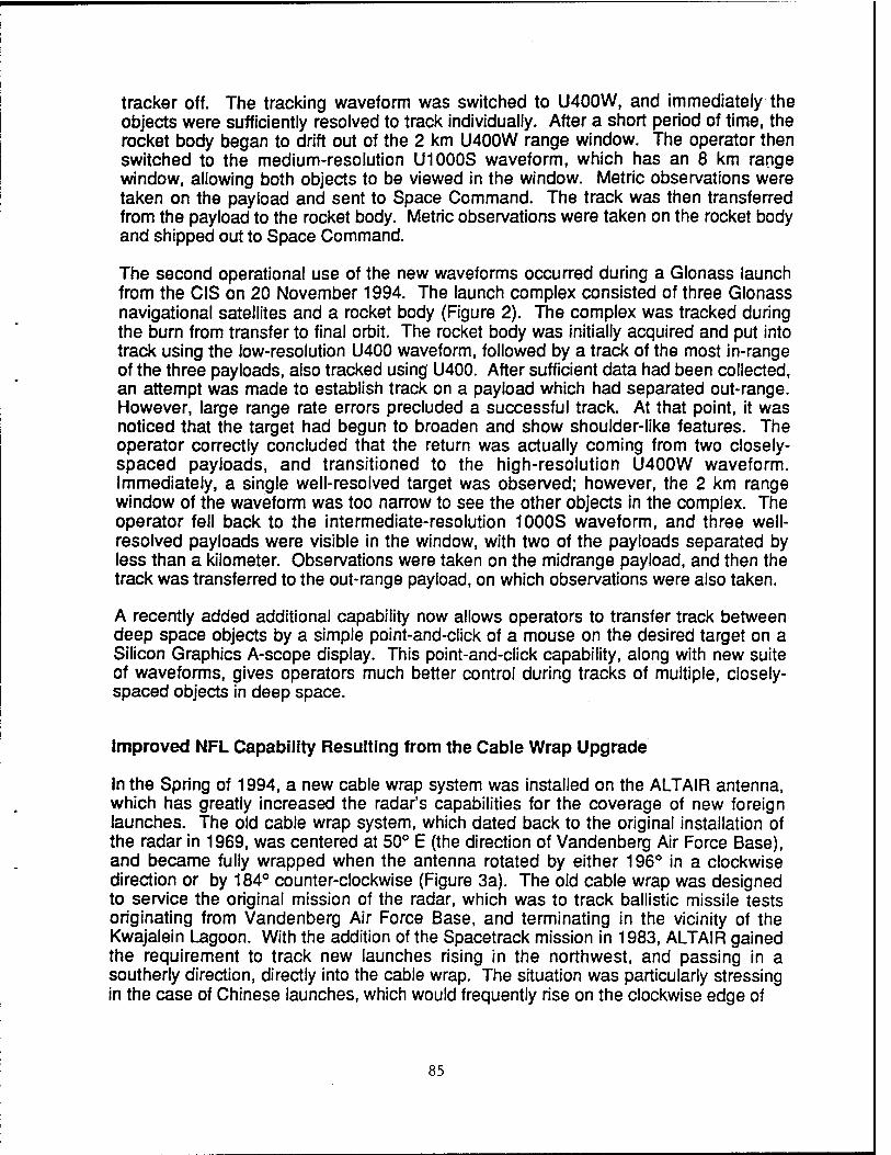
tracker off. The tracking waveform was switched to U400W, and immediately the objects were sufficiently resolved to track individually. After a short period of time, the rocket body began to drift out of the 2 km U400W range window. The operator then switched to the medium-resolution U1000S waveform, which has an 8 km range window, allowing both objects to be viewed in the window. Metric observations were taken on the payload and sent to Space Command. The track was then transferred from the payload to the rocket body. Metric observations were taken on the rocket body and shipped out to Space Command.

The second operational use of the new waveforms occurred during a Glonass launch from the CIS on 20 November 1994. The launch complex consisted of three Glonass navigational satellites and a rocket body (Figure 2). The complex was tracked during the burn from transfer to final orbit. The rocket body was initially acquired and put into track using the low-resolution U400 waveform, followed by a track of the most in-range of the three payloads, also tracked using U400. After sufficient data had been collected, an attempt was made to establish track on a payload which had separated out-range. However, large range rate errors precluded a successful track. At that point, it was noticed that the target had begun to broaden and show shoulder-like features. The operator correctly concluded that the return was actually coming from two closely- spaced payloads, and transitioned to the high-resolution U400W waveform. Immediately, a single well-resolved target was observed; however, the 2 km range window of the waveform was too narrow to see the other objects in the complex. The operator fell back to the intermediate-resolution 1000S waveform, and three well- resolved payloads were visible in the window, with two of the payloads separated by less than a kilometer. Observations were taken on the midrange payload, and then the track was transferred to the out-range payload, on which observations were also taken.

A recently added additional capability now allows operators to transfer track between deep space objects by a simple point-and-click of a mouse on the desired target on a Silicon Graphics A-scope display. This point-and-click capability, along with new suite of waveforms, gives operators much better control during tracks of multiple, closely- spaced objects in deep space.

Improved NFL Capability Resulting from the Cable Wrap Upgrade

In the Spring of 1994, a new cable wrap system was installed on the ALTAIR antenna, which has greatly increased the radar's capabilities for the coverage of new foreign launches. The old cable wrap system, which dated back to the original installation of the radar in 1969, was centered at 50° E (the direction of Vandenberg Air Force Base), and became fully wrapped when the antenna rotated by either 196° in a clockwise direction or by 184° counter-clockwise (Figure 3a). The old cable wrap was designed to service the original mission of the radar, which was to track ballistic missile tests originating from Vandenberg Air Force Base, and terminating in the vicinity of the Kwajalein Lagoon. With the addition of the Spacetrack mission in 1983, ALTAIR gained the requirement to track new launches rising in the northwest, and passing in a southerly direction, directly into the cable wrap. The situation was particularly stressing in the case of Chinese launches, which would frequently rise on the clockwise edge of

85

a)

W270*

24E*. CWELECTRC

LMT

226* OCWELECnUC

LWtr

VANOENBERG 0* CABLE WRAP

90* E

b)

N or

0* CABLE WRAP

W270*

248* CWELECTWC

LMT

CCW ELECTRIC UMfT zr

VANDENBERG 50*

90* E

Figure 3. a) Old cable wrap range of motion was 380°, centered at 50.3° (towards Vandenberg AFB). Most CCW satellite passes caused the antenna to hit the CCW cable wrap limit. (Note: The shaded area on the above figure is the servo limit region, where the antenna must slow down.) b) The new cable wrap range of motion is 576°, centered at 320° (90° CCW from Vandenberg AFB). This cable wrap orientation allows unrestricted coverage of all NFL events and satellite tracks.

86

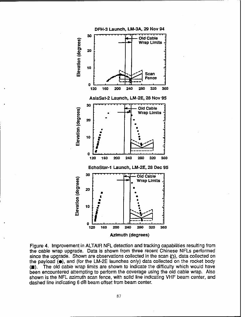
CO

8 o

to >

HI

V) a> cu h- O) CD

■o

5 .2 HI

0) V 1— D) 0>

■o

CO >

UJ

DFH-3 Launch , LM-3A, 29 Nov 94

30 — Old Cable

Wrap Limits -

20 -

10

>^.<xj Scan j ^s.-^^ I Fen«»

n r tz

120 160 200 240 280 320 360

AslaSat-2 Launch, LM-2E, 28 Nov 95 30

20

10

• ~■"™"

■ ■

■ ■ ■ ■ I I t

— Old Cable Wrap Limits :

• •

4^ i j

120 160 200 240 280 320 360

EchoStar-1 Launch, LM-2E, 28 Dec 95 30

« — Old Cable Wrap Limits :

• • •

• •

20

10

■ l ■ ■

■ f

1 n

I—_t—I

120 160 200 240 280 320 360

Azimuth (degrees)

Figure 4. Improvement in ALTAIR NFL detection and tracking capabilities resulting from the cable wrap upgrade. Data is shown from three recent Chinese NFLs performed since the upgrade. Shown are observations collected in the scan (Q), data collected on the payload (•), and (for the LM-2E launches only) data collected on the rocket body (■). The old cable wrap limits are shown to indicate the difficulty which would have been encountered attempting to perform the coverage using the old cable wrap. Also shown is the NFL azimuth scan fence, with solid line indicating VHF beam center, and dashed line indicating 6 dB beam offset from beam center.

87

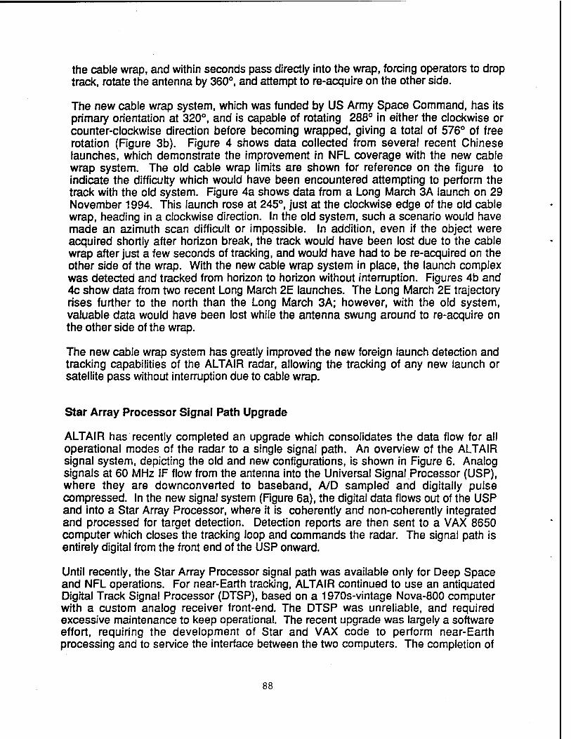
the cable wrap, and within seconds pass directly into the wrap, forcing operators to drop track, rotate the antenna by 360°, and attempt to re-acquire on the other side.

The new cable wrap system, which was funded by US Army Space Command, has its primary orientation at 320°, and is capable of rotating 288° in either the clockwise or counter-clockwise direction before becoming wrapped, giving a total of 576° of free rotation (Figure 3b). Figure 4 shows data collected from several recent Chinese launches, which demonstrate the improvement in NFL coverage with the new cable wrap system. The old cable wrap limits are shown for reference on the figure to indicate the difficulty which would have been encountered attempting to perform the track with the old system. Figure 4a shows data from a Long March 3A launch on 29 November 1994. This launch rose at 245°, just at the clockwise edge of the old cable wrap, heading in a clockwise direction. In the old system, such a scenario would have made an azimuth scan difficult or impossible. In addition, even if the object were acquired shortly after horizon break, the track would have been lost due to the cable wrap after just a few seconds of tracking, and would have had to be re-acquired on the other side of the wrap. With the new cable wrap system in place, the launch complex was detected and tracked from horizon to horizon without interruption. Figures 4b and 4c show data from two recent Long March 2E launches. The Long March 2E trajectory rises further to the north than the Long March 3A; however, with the old system, valuable data would have been lost while the antenna swung around to re-acquire on the other side of the wrap.

The new cable wrap system has greatly improved the new foreign launch detection and tracking capabilities of the ALTAIR radar, allowing the tracking of any new launch or satellite pass without interruption due to cable wrap.

Star Array Processor Signal Path Upgrade

ALTAIR has recently completed an upgrade which consolidates the data flow for all operational modes of the radar to a single signal path. An overview of the ALTAIR signal system, depicting the old and new configurations, is shown in Figure 6. Analog signals at 60 MHz IF flow from the antenna into the Universal Signal Processor (USP), where they are downconverted to baseband, A/D sampled and digitally pulse compressed. In the new signal system (Figure 6a), the digital data flows out of the USP and into a Star Array Processor, where it is coherently and non-coherently integrated and processed for target detection. Detection reports are then sent to a VAX 8650 computer which closes the tracking loop and commands the radar. The signal path is entirely digital from the front end of the USP onward.

Until recently, the Star Array Processor signal path was available only for Deep Space and NFL operations. For near-Earth tracking, ALTAIR continued to use an antiquated Digital Track Signal Processor (DTSP), based on a 1970s-vintage Nova-800 computer with a custom analog receiver front-end. The DTSP was unreliable, and required excessive maintenance to keep operational. The recent upgrade was largely a software effort, requiring the development of Star and VAX code to perform near-Earth processing and to service the interface between the two computers. The completion of

88

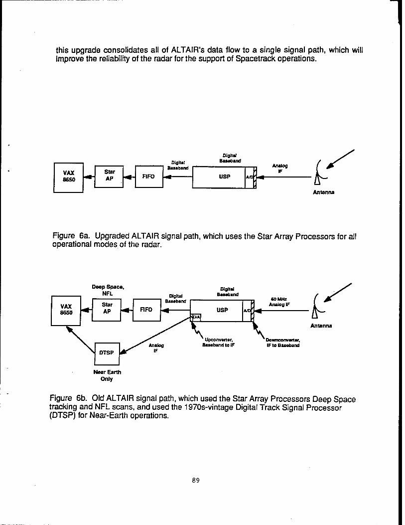
this upgrade consolidates ail of ALTAIR's data flow to a single signal path, which wil improve the reliability of the radar for the support of Spacetrack operations.

Digital Basaband

Digital Basaband

VAX 8650

Analog IF Star

AP FIFO USP A/D'^- < < i-'

Antenna

Figure 6a. Upgraded ALTAIR signal path, which uses the Star Array Processors for all operational modes of the radar.

Deep Space, NFL

Digital Basaband

VAX 8650

Star AP FIFO

Basaband

USP SS}

A/D Analog IF

v Upconvarter. Basaband to IF

\ ,0^ Analog

IF

\ Downconvsrtsr,

\ DTSP *S IF to Basaband

Near Eartr Only

i

i-' Antenna

Figure 6b. Old ALTAIR signal path, which used the Star Array Processors Deep Space tracking and NFL scans, and used the 1970s-vintage Digital Track Signal Processor (DTSP) for Near-Earth operations.

89

Communications Processor Upgrade

The communications processor which processes message traffic between the Kwajaiein Missile Range ALTAIR, ALCOR and MMW radars and Space Command at Cheyenne Mountain is being upgraded. The reasons for the upgrade are: (i) the need to replace the Kwajaiein Communications Center's S130 computer, which currently performs the processing and is at the end of its life cycle, (ii) to support the joint Air Force/Navy requirement to install a dedicated circuit to the Alternate Space Surveillance Center (ASCC) at Dahlgren, VA, and (iii) to support the Army's transition to a Message Distribution Terminal (MDT) interface for AUTODIN message traffic.

The architectures for the current and upgraded communications paths are shown in Figure 5. In the current system, message traffic from the ALTAIR, ALCOR and MMW radars is sent to the Kwajaiein Communications Center, where it is reformatted in either ADCCP or AUTODIN format on the S130 computer, and uplinked to a DSCS satellite. ADCCP traffic is downlinked at Camp Roberts, CA, and sent via commercial trunk line to the Cheyenne Mountain Communations Systems Segment (CSS). The CSS distributes ALTAIR messages to the Space Control Center (SCC), and ALCOR/MMW images via the Intelligence Data Handling System (IDHS) to the Combined Intelligence Center (CJC), the end users of the data. The AUTODIN circuit provides partial redundancy to the ADCCP circuit. AUTODIN traffic is downlinked at Wahiwa, HI, where it is distributed to users including the CSS and the Millstone Hill radar.

The new message processor will reside on a micro-VAX computer at ALTAIR, and will incorporate all message processing functions previously performed by the ALTAIR Message Processing Program (AMPP) and the S130 computer. ADCCP-formatted messages generated at ALTAIR will be output to a four-way time multiplex device, which will fill one slot for transmission of data to the SCC, and a second slot with identical data for transmission to the ASCC at Dahlgren. ALCOR/MMW imaging data will be multiplexed into the third slot, while the fourth slot will not be used. The data will be uplinked to the DSCS satellite, and downlinked at Falcon AFB, where it will be de- multiplexed. Two ADCCP circuits, one for ALTAIR messages and one for ALCOR messages, will be run to the CSS in Cheyenne Mountain, while a third ADCCP circuit will carry ALTAIR messages to the ASCC at Dahlgren.

The communications processor upgrade is expected to be complete in the third quarter of FY96. When completed, the new system will greatly improve the reliability of the communications path between KMR and space surveillance data users, while providing the required dedicated circuit between ALTAIR and the ASCC.

90

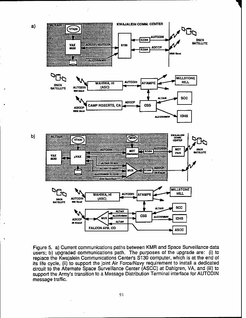
a)

*D*

KWAJALBN COMM. CENTER

V* _. WAHIWA, HI SATELLITE AUTODIN] (ASC)

600 Baud

ADCCP [

S130

.AUTODIN |.KG84| ft*

■ ADCCP Kein ■»

DSCS SATELLITE

1600 Baud

CAMP ROBERTS, CA

b)

*0* Vv D8C8

SATELLITE AUTOOIN K» Baud

WAHIWA, HI (ASC)

AUTODIN AFAUPE

ADCCP MKbaurf

MUX

ALTAID

ALCOR/MMW

ALTAR

FALCON AFB, CO

I CSS

MILLSTONE HILL

SCC

IDHS

V f» ASCC

Figure 5. a) Current communications paths between KMR and Space Surveillance data users; b) upgraded communications path. The purposes of the upgrade are: (i) to replace the Kwajalein Communications Center's S130 computer, which is at the end of its life cycle, (ii) to support the joint Air Force/Navy requirement to install a dedicated circuit to the Alternate Space Surveillance Center (ASCC) at Dahlgren, VA, and (iii) to support the Army's transition to a Message Distribution Terminal interface for AUTODIN message traffic.

91

Summary

The radars at the Kwajalein Missile Range provide the US Army component support to the US Space Command space surveillance effort. ALTAIR, as the principal KMR space surveillance radar, maintains an ongoing program of upgrades to improve its ability to perform this important mission. A recently installed set of high-resolution waveforms is now allowing the resolution, discrimination and tracking of closely-spaced objects in deep space. An upgrade to the antenna cable-wrap system is providing improved capability for the coverage of new foreign launches. Completion of a Star Array Processor signal path upgrade has consolidated near-Earth and deep space tracking operations onto a single signal path, improving the reliability and maintainability of the radar. An upgrade is underway to the communications processor used to transmit message traffic to and from Space Command, which will improve the capability and reliability of this communications link. These and other upgrades underway will continue to enhance the quality of service that ALTAIR provides to space surveillance data users.

Reference

1. S. Chapman, A. Gerber, G. Hogan, S. Hunt, R. Anderson, J, Conrad, D. Sponseller and M. Schlueter, "Recent Improvements at the ALTAIR Radar", Proceedings of the 1994 Space Surveillance Workshop, 1994.

92

NEW VHF WAVEFORM CAPABILITIES AT THE ALTAIR RADAR1

Michael E. Austin, M.I.T. Lincoln Laboratory

1. Introduction

The ALTAIR radar operates at UHF and VHF on the Kwajalein Atoll in the Republic of the Marshall Islands, as one of the major sensors of the U.S. Army Kwajalein Missile Range (KMR). Current modifications scheduled to be completed by April 1997 will provide significant new VHF waveform capabilities at ALTAIR:

Transmit / Receive Polarization Agility

Transmit /Receive Frequency Agility

• Phase-Code Modulated Pulses

• Pulse-by-Pulse Waveform Agility

• Transmit Pulse Sampling

Implementation of these new capabilities requires major modifications to the radar's VHF transmitter, coaxial components, antenna structure, and receivers. To achieve the pulse-by-pulse waveform agility and transmit pulse sampling, ALTAIR will be controlled by a new object- oriented Mode-independent Real-Time Program (MRTP) being written to replace the radar's existing real-time program. This paper provides a description of the new capabilities, the hardware modifications and software development required to bring them about, and some potential radar data collection uses to which they may be applied.

2. New Capabilities

ALTAIR presently transmits only Right-Circular (RC) pulses. When new hardware and software modifications are completed, KMR Users will be able to select either circular or linear polarization for all VHF Linear Frequency Modulated (LFM) or Phase-Code Modulated (PCM) pulses. Parameters may be set to transmit Right-Circular (RC), Left-Circular (LC), 45° Linear or 135° Linear polarization. Moreover, for VHF PCM waveforms (including CW waveforms generated as a special case of PCM), the transmit polarization may be switched at the midpoint of a pulse. This permits, for example, transmitting a pulse with RC polarization over the first half of the pulse and with LC polarization over the second half of the pulse, or 45° Linear on the first half and 135° Linear on the second half. While transmitting a pulse having both circular and linear polarization is possible, the time required to reconfigure receive hardware precludes such a mixture. ALTAIR's VHF receiver can provide both PP and OP sum-channel samples and LC traverse-difference and LC elevation-difference channel samples for any transmit polarization (the difference channels are down 3 dB when using linear polarization).

93

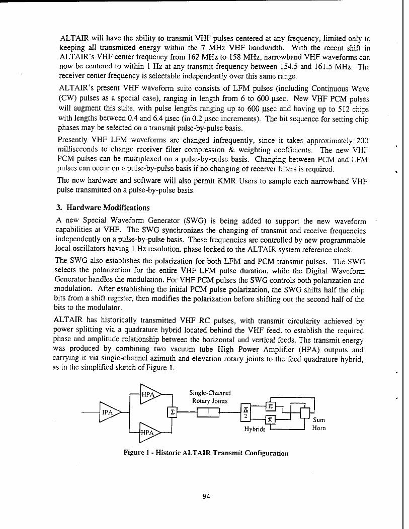
ALT AIR will have the ability to transmit VHF pulses centered at any frequency, limited only to keeping all transmitted energy within the 7 MHz VHF bandwidth. With the recent shift in ALTAIR's VHF center frequency from 162 MHz to 158 MHz, narrowband VHF waveforms can now be centered to within 1 Hz at any transmit frequency between 154.5 and 161.5 MHz. The receiver center frequency is selectable independently over this same range.

ALTAIR's present VHF waveform suite consists of LFM pulses (including Continuous Wave (CW) pulses as a special case), ranging in length from 6 to 600 jisec. New VHF PCM pulses will augment this suite, with pulse lengths ranging up to 600 jisec and having up to 512 chips with lengths between 0.4 and 6.4 jisec (in 0.2 |isec increments). The bit sequence for setting chip phases may be selected on a transmit pulse-by-pulse basis.

Presently VHF LFM waveforms are changed infrequently, since it takes approximately 200 milliseconds to change receiver filter compression & weighting coefficients. The new VHF PCM pulses can be multiplexed on a pulse-by-pulse basis. Changing between PCM and LFM pulses can occur on a pulse-by-pulse basis if no changing of receiver filters is required.

The new hardware and software will also permit KMR Users to sample each narrowband VHF pulse transmitted on a pulse-by-pulse basis.

3. Hardware Modifications

A new Special Waveform Generator (SWG) is being added to support the new waveform capabilities at VHF. The SWG synchronizes the changing of transmit and receive frequencies independently on a pulse-by-pulse basis. These frequencies are controlled by new programmable local oscillators having 1 Hz resolution, phase locked to the ALTAIR system reference clock.

The SWG also establishes the polarization for both LFM and PCM transmit pulses. The SWG selects the polarization for the entire VHF LFM pulse duration, while the Digital Waveform Generator handles the modulation. For VHF PCM pulses the SWG controls both polarization and modulation. After establishing the initial PCM pulse polarization, the SWG shifts half the chip bits from a shift register, then modifies the polarization before shifting out the second half of the bits to the modulator.

ALTAIR has historically transmitted VHF RC pulses, with transmit circularity achieved by power splitting via a quadrature hybrid located behind the VHF feed, to establish the required phase and amplitude relationship between the horizontal and vertical feeds. The transmit energy was produced by combining two vacuum tube High Power Amplifier (HPA) outputs and carrying it via single-channel azimuth and elevation rotary joints to the feed quadrature hybrid, as in the simplified sketch of Figure 1.

Single-Channel Rotary Joints

lit 2

ZLT-L K

Hybrids

Sum Horn

Figure 1 - Historic ALTAIR Transmit Configuration

94

Achieving pulse-by-pulse polarization agility presented a technical challenge and resulted in the most visible hardware modifications. In the late 1980's a high-power mechanical coax switch was temporarily installed behind the VHF feed to allow LC polarization transmissions by switching the power to the alternate quadrature hybrid input port. Mechanical high-power polarization switching required a few seconds, and could not support the desired pulse-by-pulse switching. It was suggested by Guy Huse of MIT/LL to use low-power switching of the phase relationships of signals driving the two HP As, as shown in Figure 2. Transmitted pulses will be 45° Linear polarization when the phase shifter is set for 0°, Right-Circular polarization for 90°, 135° Linear polarization for 180° and Left-Circular polarization for -90°. In the original configuration of Figure 1, reflections from the coaxial components and feed hybrids were absorbed via a load (not shown) on the hybrid used to sum the two HPA outputs. In the new configuration each HPA output goes directly to the feed hybrids, and reflections are absorbed in the terminations of two new VHF circulators. The circulators each weigh about 1800 pounds.

Dual-Channel Rotary Joints

Circulators

Lj LZLi-T

J~l K

Hybrids

Sum Horn

Figure 2 - New ALTAIR Transmit Configuration

In addition to controlling the HPA input phase relationships, their output power levels need to match closely over the entire band. Digitally controlled phase shifters and new Intermediate Power Amplifiers (IPAs) were procured to achieve the phase and amplitude stability. The IPAs were found to phase track to within 0.75° over the entire VHF band, which coupled with the HPA output power matching to within 0.5 dB should yield a transmit polarization ratio of about 30 dB.

Figure 3 - Old and New ALTAIR Antenna Structure

95

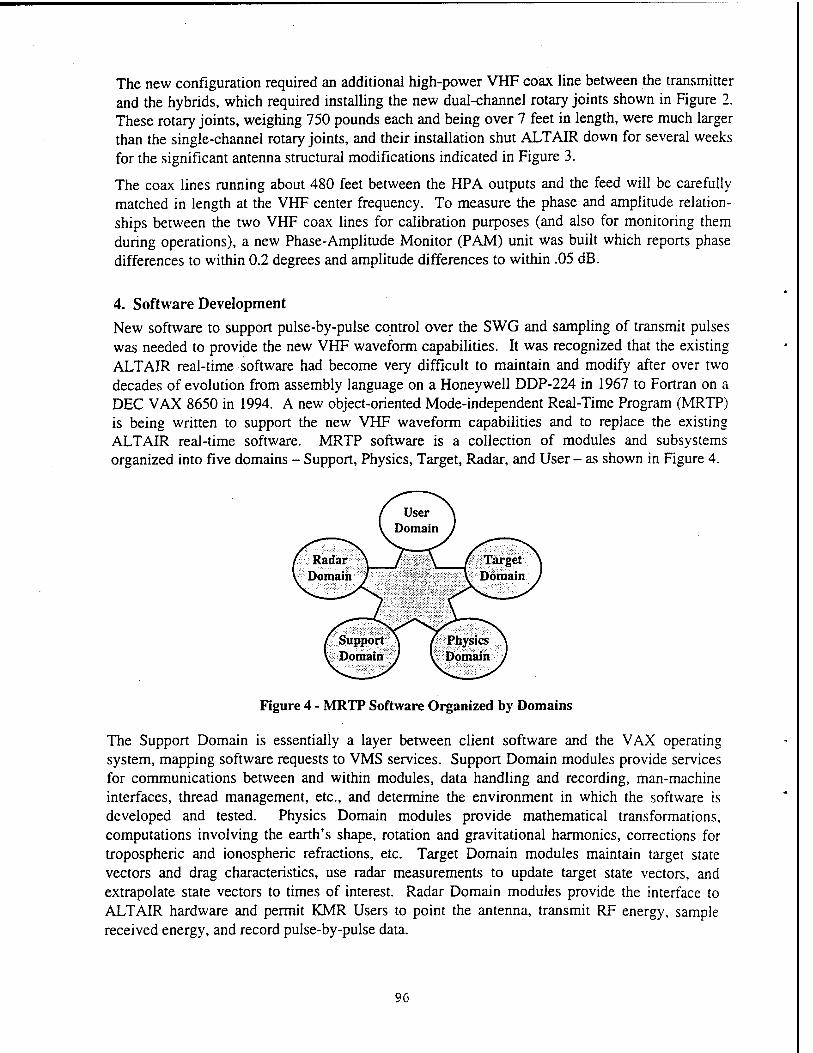
The new configuration required an additional high-power VHF coax line between the transmitter and the hybrids, which required installing the new dual-channel rotary joints shown in Figure 2. These rotary joints, weighing 750 pounds each and being over 7 feet in length, were much larger than the single-channel rotary joints, and their installation shut ALT AIR down for several weeks for the significant antenna structural modifications indicated in Figure 3.

The coax lines running about 480 feet between the HPA outputs and the feed will be carefully matched in length at the VHF center frequency. To measure the phase and amplitude relationships between the two VHF coax lines for calibration purposes (and also for monitoring them during operations), a new Phase-Amplitude Monitor (PAM) unit was built which reports phase differences to within 0.2 degrees and amplitude differences to within .05 dB.

4. Software Development

New software to support pulse-by-pulse control over the SWG and sampling of transmit pulses was needed to provide the new VHF waveform capabilities. It was recognized that the existing ALT AIR real-time software had become very difficult to maintain and modify after over two decades of evolution from assembly language on a Honeywell DDP-224 in 1967 to Fortran on a DEC VAX 8650 in 1994. A new object-oriented Mode-independent Real-Time Program (MRTP) is being written to support the new VHF waveform capabilities and to replace the existing ALTAIR real-time software. MRTP software is a collection of modules and subsystems organized into five domains - Support, Physics, Target, Radar, and User - as shown in Figure 4.

Figure 4 - MRTP Software Organized by Domains

The Support Domain is essentially a layer between client software and the VAX operating system, mapping software requests to VMS services. Support Domain modules provide services for communications between and within modules, data handling and recording, man-machine interfaces, thread management, etc., and determine the environment in which the software is developed and tested. Physics Domain modules provide mathematical transformations, computations involving the earth's shape, rotation and gravitational harmonics, corrections for tropospheric and ionospheric refractions, etc. Target Domain modules maintain target state vectors and drag characteristics, use radar measurements to update target state vectors, and extrapolate state vectors to times of interest. Radar Domain modules provide the interface to ALTAIR hardware and permit KMR Users to point the antenna, transmit RF energy, sample received energy, and record pulse-by-pulse data.

96

User Domain modules are designed to meet the data collection requirements of KMR Users, and rely heavily on services from the other Domains. For each User a customized "Script" module controls transmit pulse characteristics, receive sampling parameters, and data recording via Radar Domain services, while tracking targets via Target Domain services. User Domain modules are responsible for processing all samples obtained from the Radar Domain in order to meet the User's specific search, measurement, track and data collection requirements.

Data Collection Interval 2

Figure 5 - MRTP Data Collection Intervals

Ideally KMR Users could specify information prior to an operation regarding the target complex and the pulse types to be used, and then exercise complete control over all of the ALTAIR's capabilities on a pulse-by-pulse basis. This is almost possible, however, some radar capabilities require time to reconfigure, such as switching between LFM and PCM modulation, switching the receiver front end hybrid matrix between linear and circular polarization, changing the receive pulse compression and weighting filter coefficients, etc. Due to such reconfiguration requirements, MRTP utilizes Data Collection Intervals (DCIs) as sketched in Figure 5. For each DCI the User specifies Start- and Stop-Criteria (based on target range, elevation, altitude, time, etc.), plus those slow-to-reconfigure system parameters to be held constant during the DCI. Within a DCI the User specifies antenna pointing, transmit pulse parameters, and receive sampling parameters on a pulse-by-pulse basis. DCIs enforce the need for Users to consider hardware configuration requirements in their mission planning.

MRTP is expected to benefit KMR and its Users in two ways. The first benefit is a direct result of the object-oriented approach used for MRTP development. The emphasis on data encapsula- tion and client-independent module services will make software maintenance and modification straightforward, and it will be much easier to add new capabilities to ALT AIR than with the existing real-time software. The second benefit is that when new KMR User requirements arise, they can be efficiently handled by creating a new Script module in the User Domain, without the time and expense of having to modify modules in the other domains.

5. New Data Collection Capabilities

The new VHF capabilities and pulse-by-pulse flexibility will provide KMR Users with new potential data collection opportunities. Pulse-by-pulse or mid-pulse polarization switching will support measurements of the full scattering matrix of targets - using circular and/or linear polarization - which will allow better characterization and identification of targets.

97

Ground-based measurements at VHF are typically conducted on outdoor ground-reflection ranges which cannot support circularly-polarized measurements. Linear polarization capability at ALT AIR will provide actual flight data for comparison with ground data, and may aid in the evaluation of such outdoor range errors.

The new hardware and software also provide pulse-by-pulse agility in the VHF transmit and receive center frequencies. This frequency agility, combined with polarization flexibility, will allow KMR Users to completely characterize the scattering properties of targets at any desired frequencies within ALT AIR's 7-MHz VHF band.

Frequency agility and polarization switching can be used during tracking to mitigate signal fading caused by nulls in a target's radar cross-section pattern. Frequency agility also permits users to account for target motion by correcting for doppler on either transmit or receive.

ALTAIR's equatorial location and VHF operating frequency have historically made it a major contributor in the area of ionospheric physics. KMR Users will be able to utilize long PCM waveforms with short chips to obtain high energy pulses, which can be processed to provide detailed phase and amplitude perturbations due to the ionosphere. Processed returns will have good range resolution after processing, and such pulses will be useful in studying ionospheric backscatter, for example, where small range cells and doppler cells are simultaneously desired. Script algorithms are being coded which will permit processing of the individual chips in a PCM pulse, affording the capability to accurately assess propagation phenomena.

With KMR User scripts providing control over multiple Data Collection Intervals (DCIs) during a mission, a single mission could collect scattering matrix during one DCI, study the frequency response for a given polarization on another DCI, and still collect data over a wide range of modulations for a fixed frequency and polarization during other DCIs. By interspersing long PCM waveforms sampled in-range of the target, the characteristics of scintillation could be recorded.

The ALTAIR radar is being equipped with unique capabilities, unavailable at any other instrumentation radar, which can be easily controlled by KMR Users. We challenge those in the scientific community to utilize ALTAIR's new capabilities in previously unimagined ways to satisfy their numerous and diverse measurement requirements.

Acknowledgments

The extensive hardware and software modifications to ALTAIR described in this paper are being implemented and tested by a joint CONUS-Site team of systems, hardware and software engineers from M.I.T. Lincoln Laboratory (LL), Range Systems Engineering (RSE), and GTE Government Systems Corp. Among the major contributors to the transmitter, microwave and antenna modifications were Guy Huse, Ralph MaruIIi and Royal Purdy of LL, and Robert Anderson, Thin Ng and Mark Schlueter of RSE' Hardware design, construction and testing of the SWG and PAM units were largely the work of John Giarratano of RSE. MRTP software is being implemented by Bevan Jacobs, Wallace Schubach, Thomas Melia and Paul Masciarelli, aided by Richard Marshall and Himangshu Bhattacharya, all of RSE, and Robert McHugh of GTE. The MRTP design principles are those proposed by the project's late software leader, Wayne Trombini of GTE, as expressed in specifications prepared by Louis Jankauskas of GTE, John Giarratano and Arthur Lewis of RSE, and Marcia Powell of LL. Site MRTP testing at ALTAIR is being done by Gregg Hogan of LL.

98

GEODSS Upgrade Prototype System (GUPS) Program Status

Dr. C. Max Williams (TRW), Sam D. Redford (TRW)

1. Introduction and Summary

The Ground-based Electro-Optical Deep Space Surveillance (GEODSS) System provides critical metric and Space Object Identification (SOI) observation data on deep space satellites to the Space Control Center (SCC) in Cheyenne Mountain. GEODSS concepts and development occurred in the 1970s and it became operational in the early 1980s. It was based on the 1970s technology including sensor, signal processing algorithms and hardware, and data processors and languages.

The GEODSS Upgrade Prototype System- (GUPS) is a 3 year technology insertion program and is a part of the Space Surveillance Network Improvement Program (SSNIP). GUPS was procured by the Air Force Sacramento Air Logistics Center (SM-ALC), is technically managed by the Electronic Systems Center (ESC) and performed by TRW, Inc. GUPS will demonstrate the applicability of several technological advances to the GEODSS system. The new technologies include high performance Charge-Coupled Device (CCD) sensors, enhanced signal processing and tracking algorithms, and modem data processing equipment and languages. Many of these technological advances are directly attributable to MIT/Lincoln Laboratory (MIT/LL) research programs. The resulting system will have greatly improved sensor performance, with higher sensitivity (able to detect objects 2 visual magnitudes dimmer), better metric accuracy, and the ability to search twice as fast and track twice as many objects as a current GEODSS sensor.

GUPS is also developing an Exclusion Zone Sensor (EZS) which will provide an automated method of determining which areas of the sky are acceptable for observations. The GUPS program will also demonstrate repeatability, and that the GUPS can be transported by land, sea or air, and can be deployed worldwide within months. Figure 1 illustrates a two-telescope relocatable GUPS system.

The GUPS program was planned with several demonstrations at the GEODSS Test Site (GTS) to demonstrate ongoing progress. These demonstration feature the relocatability and the improved sensor performance. These demos are:

Demo 1 Successful telescope deployment on/off pedestal Nov ' 94 Demo 2 Successful sidereal tracking with ebsicon sensor June '95 Demo 3 Successful searching and tracking with CCD sensor Jan '96 Demo 4 Planned demonstration of EZS sensor Mar '96 Demo 5 Planned demonstration of entire GUPS system Jan '97

To date, the GUPS program has been very successful in the design, development and demonstration of system capability. We do not see any major problems which could prevent GUPS from providing all the desired capabilities.

GUPS is expected to continue as a testbed for new technologies prior to use in the operational system. Capabilities proven in GUPS are planned to be incorporated in the GEODSS Modernization Program (GMP) which will upgrade the existing GEODSS system. The GUPS relocatable system itself may also be deployed overseas; this would provide a very quick and cost effective enhancement to operational space surveillance in areas where coverage does not currently exist. In addition, because of the high sensitivity of the new CCD, GUPS could support the Near Earth Asteroid detection mission.

99

Figure 1. A Deployed - Relocatable GUPS

2. History and Legacy of GEODSS / GUPS

The anticipated GUPS sensor capabilities and improved sensor performance are attributable to both the GEODSS system and recent technology developments at MIT/LL. Research for the GEODSS system began in the early 70s, and involved ESC, MIT/LL and TRW. A contract was awarded to TRW in 1978 to develop and install operational sites at Socorro, Maui, Diego Garcia, and Korea (now deactivated). The sites provide both metric observations and SOI data on deep space objects to the SCC. GEODSS uses a 40 inch main telescope and polar mount developed by Contraves; the same telescope will also be used in the GUPS system. GEODSS uses an ebsicon tube as its sensor, and processes binary data using an elementary sidereal tracking algorithm. Significant improvements have occurred in sensor and signal processing methods since the initial GEODSS development.

During the last few years, there have been many advances for electro-optical sensor technology. In addition to the development of the CCD itself (discussed later), MIT/LL has been involved in the development of the Space-Based Visible (SBV) sensor on the MSX satellite; the GUPS sidereal detection algorithm is derived from SBV detection methods.

3. Relocatable Shelters

The relocatable GUPS, illustrated in figure 1, is being developed such that the complete system can be dismantled, transported by land, sea, or air (Air Force C-141), and deployed to a previously unprepared worldwide site within six months of deployment decision. Upon arrival at a prepared site, the relocatable GUPS can have the telescope mounted and associated mission equipment functioning within a few weeks. The design of the relocatable GUPS is based upon International Standardization Organization (ISO) transportable shelters and trailers which have an extensive history in mobile and transportable military applications. The GUPS relocatable system incorporates one Telescope Shelter, one Operations Shelter, a custom trailer with hydraulic lifting devices, and an existing GFE GEODSS observation dome and

100

EZS OPERATIONS

SHELTER TELESCOPE SHELTER

Operator Consoles Video Dlsplay/VCR Comm Equipment ADPE for DPS (Data Processing and Scheduling)

■ EZS Processor

Power Video Ethernet Sensor Commands/ Reponaea

- Maintenance Console - ADPE for Sensor Controller - Signal Processor - Mount Controller Electronics

- GEODSS Dome - Telescope/Mount - CCD Camera

Figure 2. GUPS Operations and Telescope Shelters

dome base, as illustrated in figure 2. In addition, GUPS has been designed to easily accommodate expanded mission requirements whereby each Operations Shelter can control up to 4 Telescope Shelters. The relocatable GUPS is capable of being deployed in both the northern and southern hemispheres at site locations between + or - 45 degrees latitude. The GUPS Telescope Shelter is designed to allow the transfer of the telescope from the shelter to a rigid pedestal without the need for special support equipment at the site. Figure 3 is an illustration of the

Figure 3. Transfer of Telescope to GUPS Pedestal

transfer of the telescope to the pedestal from Demo 1; this process required approximately 30 minutes. In addition, the telescope was removed from the pedestal and secured back in the telescope trailer in approximately 30 minutes.

101

4. Sensor Controller Subsystem

The most complex element of the GUPS program is the development of the Sensor Controller Subsystem. Figure 2 illustrates the Telescope Shelter which physically contains the Sensor Controller including the general purpose data processor and the signal processor hardware which process image data from the CCD camera. The Operations Shelter houses the Data Processor and Scheduling (DPS) Subsystem which supports the operator displays, communications equipment, catalog maintenance and the task scheduler for the system. A single DPS subsystem is capable of controlling up to 4 sensors.

The DPS software in the Operations Shelter will transmit high level commands to the Sensor

Controller, such as:

- Search in given area and report on any observed detections, - Search for a known object at a predicted location and rates, - Acquire and track a known object for x seconds, or - Collect SOI data for x seconds on an object in track.

This simple, straightforward command interface to the Sensor Controller also facilitates remote control of a sensor by a distant site such as the Optical Command Control Communications Facility (OC3F) which will be developed on GMP. In the remote operations mode, commands from the OC3F would effectively "pass through" the local DPS to the Sensor Controller and metric and SOI observation data would pass through the local DPS back to the remote OC3F. This remote control capability will be demonstrated on the GUPS program during Demo 5.

Although many of the new GUPS concepts were developed to take advantage of the high performance CCD sensor, the GUPS Sensor Controller and its signal processing architecture and tracking algorithms can be used with the existing ebsicon tube. Demo 2, which occurred in June 1995, was the first GUPS sensor demo and it used the ebsicon tube to successfully perform sidereal detection and tracking.

There are many elements in GUPS, but three particularly important elements are the CCD chip and camera, detection processing algorithms, and the signal processing architecture to process the large volume of CCD sensor data.

4.1 CCD Chip and Camera

The most important technology insertion element in GUPS is the large-format CCD sensor. It will provide significantly improved sensor performance over the current ebsicon sensor. The CCD chip was produced by MIT/LL and the CCD camera was developed by Photometries Corporation. The CCD chip, illustrated in figure 4, is a large 1960 x 2560 array having over 5 million pixels. It has high resolution with each pixel corresponding to a 2x2 arcsecond area, it is back-illuminated and has a quantum efficiency exceeding 0.65. It is a frame transfer device, has 8 output ports and can be readout in 0.36 seconds (readout in less than 0.17 sec for binned data). The CCD device also has a 32x32 photometric subarray which is used for SOI data collection.

The first production CCD camera was delivered to the GUPS program in July 1995. It is now installed in the telescope shelter at the GTS and is being actively used for integration testing and for demonstrations. The camera uses thermoelectric cooling and fluid cooling to lower the

102

Figure 4. CCD Chip Developed by MIT/LL For GUPS

sensor temperature to -50 degrees Centigrade and thus minimize thermal noise in the CCD sensor. The camera can be commanded to take long exposures up to 100 seconds; this would support the asteroid detection mission which must detect near earth objects as faint as 22nd visual magnitude.

4.2 Detection Processing and Tracking Algorithms for Metric Observation Generation

GUPS is required to detect and track objects in two modes: sidereal tracking and target tracking. Figure 6 illustrates the two methods and addresses the advantages and disadvantages of each.

An elementary sidereal tracking method was implemented in GEODSS, but there have been many improvements over the years. Sidereal track is basically composed of two processing elements, the star background rejection and the streak detection (these are often referred to as time dependent processing and object dependent processing). For star background rejection, GUPS uses a variant of the normalized Maximum Value Projection (MVP) method developed by P. Chu at MIT/LL for use on the SBV sensor. This star background rejection method is mathematically very simple, but is computationally demanding. It must be performed on the 5 megapixel image, 3 times a second, which is approximately 30 megabytes of image data per second. Approximately 500 million floating operations per second (MFLOPs) are required to process this volume of data.

There are many approaches for streak detection algorithms which were considered for use in GUPS. These include the use of Hough transform and maximum likelihood matched velocity filtering. However, the method finally chosen for GUPS sidereal processing uses clustering / moment algorithms because of their basic simplicity and they have been operationally proven. These methods were developed on the original GEODSS program and advanced versions have been used on various spacebom sensors. The method finds clusters of nearby points which may be part of a streak and then calculates moments to determine if the distribution of the points are consistent with that of a streaking object. Angular positions and rates are then calculated.

103

SIDEREAL TRACKING TARGET TRACKING

Description: - Telescope "stares" in the direction of fixed stars - Satellites leave a "streak" over many pixels

"^ Description:

- Telescope slews at the same angular rate as moving satellite - Keeps an Object in the same Pixel (at least shorter streaks)

Figure 6. Characteristics of Sidereal and Target Track

The sidereal processing algorithm has been implemented on the GUPS signal processing hardware and successfully demonstrated on both the ebsicon sensor (at Demo 2) and the CCD sensor (Demo 3).

Current analysis indicates that the sidereal detection algorithm should be able to detect and track geosychronous objects as dim as 17.7 visual magnitudes. Because of the relatively fast camera frame rates and efficient signal processing methods, the GUPS sensor controller should be able to collect sets of metric observations on over 150 satellites each hour. Each angular metric observation should be accurate to approximately 5 arcseconds, which is limited primarily by the use of a telescope mount model. Enhancements are being considered where the sensor controller would use reference stars in the image field of view to generate more accurate observations; subpixel accuracy (1 arcsecond) should be attainable.

A disadvantage of sidereal tracking is that the object moves across many pixels and the signal to noise on each individual pixel may be too small for detection. The target tracking algorithm (also called rate track) solves this by slewing the telescope at the same rate as the object, thereby integrating the energy in a small area, achieving a much higher signal to noise ratio and thus providing a higher probability of detection. A automated detection method will be used in GUPS. It will allow GUPS to detect much dimmer objects than detectable with the sidereal detection method; in fact, geosynchronous objects as dim as 18.9 visual magnitudes should be detectable.

The rate track algorithm has been developed and coded and is in the process of integration at the GTS. This detection method should be operational in the March / April 1996 time frame. It will be featured in Demo 5.

104

After an object has been initially acquired using either the sidereal detection algorithm or the automated target track algorithm, the object can be placed into "autotrack". Autotracking involves finding the object in each frame, centroiding the intensity data from pixels containing the object, and exercising closed-loop feedback control of the telescope mount to maintain track. This tracking method will allow extended track on an object without relying on an element set. It is also used when SOI data is collected on an object.

4.3 Signal Processing Architecture

The GUPS Sensor Controller Subsystem employs a VME-based data processing architecture. The Motorola 68040 processor was chosen as the host processor because of its proven performance in many real-time applications and because of the available software for development support. However, this processor cannot perform the estimated 500 MFLOP processing required for the maximum value projection algorithm.

Several signal processing architectures were examined to perform this heavy signal processing load, including special purpose image processing hardware. The selected hardware consists of a VME based Mercury board having 16 Intel i860 processors and 256 megabytes of storage. It is a Commercial Off The Shelf (COTS) product which has been proven in many demanding signal processing applications and provides the flexible software environment needed in GUPs. It has a real-time operating system, supports software written in the C language, and has high data rate internal buses to receive and process image data.

Figure 7 depicts a notional architecture of 15 i860 processors to process the CCD images; only 4 processors are required to process the small ebsicon images.

► Processor 1 " -

CCD Camera 16MBYTES/SEC

Receive Data —^ Compensate

»> Processor 12

|

1 ► i—L

• L— GEN fl Metric Obs 1"

1 dMBYTES/SeCi , ===== • • =d 1 ■* Receive

Data ** Compensate

Functions:

Processor #8

Collect Pixel Statistics Normalize Maximum Values Bin or Convolve Data Threshold Pixel Data Determine Clusters Calculate Moments

Note: Each Box represents an i860 processor with associated memory

1-

Figure 7. GUPS Signal Processing Architecture

105

As stated earlier, this signal processing architecture has been implemented and proven. The 4 processor version was used in Demo 2 with the ebiscon sensor and the 16 processor version successfully processed the 30 megabytes / second image data from the CCD camera in Demo 3. Analysis also indicates that this configuration will be able to process the SOI photometry images at 1000 hertz without any problem.

4.4 SOI Data Collection

The CCD chip and camera support the collection of multi-color Space Object Identification (SOI) data in addition to collecting metric observations. The chip has a 32x32 photometric array for collection of SOI data and the CCD camera has actually collected images at over 1300 frames per second in the binned mode.

A GUPS goal is to collect SOI data at over 1000 samples per second and also to estimate the intensity of each sample accurately to 0.25 Visual Magnitudes. To accomplish this, the sensor controller utilizes a "software aperture " on the image. This consists of, for example, a 5x5 square pixel area surrounding the object's expected location. The object's intensity is estimated by summing the total intensity in the SW aperture and subtracting out the estimated background level. A single i860 processor will be used to perform this processing on 1000 photometer images each second.

GUPS will also employ BVRI spectral filters over the array allowing collection of multi-spectral SOI data. These spectra are for blue (B), visible (V), red (R) and infrared (I). Broadband SOI can also be collected in the open position where no filter is used. GUPS will perform an accurate multispectral "instrument calibration" using the UBVRI calibration star catalog developed by Dr. Arlo Landolt of LSU; an instrument calibration determines the color dependent zero value and color transformation coefficients. In addition, GUPs can perform a nightly "extinction calibration" to determine the current primary and secondary color dependent atmospheric extinction coefficients. Having an accurate calibration will, of course, ensure that the operational SOI data will be more accurate.

In order to collect SOI data, the Sensor Controller will first detect the object on the main array, autotrack it, and finally adjust the mount slewing rates so that the object appears on the 32x32 subarray. Closed-loop autotracking will continue on the subarray during SOI data collecting. Autotracking allows the collection of SOI over extended time intervals.

The SOI processing methods have been designed are currently being implemented. These capabilites will be integrated and tested at the GTS by March / April 1996 and will be shown in Demo 5.

5. Exclusion Zone Sensor

The GUPS program is also developing an Exclusion Zone Sensor (EZS) which determines sky visibility data at the local sensor site. The EZS will generate a map of cloudy areas over the sensor site. This data is transmitted to the scheduler so that it can determine those sky areas where objects can be successfully tracked and areas which should be avoided. For remotely controlled systems, the EZS mapping data can be transmitted to the remote control location for use in its scheduler.

106

Figure 8 shows an image from the EZS camera using the 8 mm Olympus fisheye lens. The grid pattern depicts the sectors which have been defined for EZS. The final sector map will indicate if a sector is visible or not, along with the estimated skybackground and extinction value in the sector. Optionally, the EZS can also output a highly compressed image (40K bytes) which can be displayed locally or transmitted over high bandwidth communication lines.

Figure 8 EZS Image with Sector Map Overlay

The EZS system consists of an Astromed camera with a 1024x1280 CCD and an 8mm lens. A special device called a "moon occulter" is used to block moon light from the lens in order to prevent saturation or glare in the camera. A Sun Sparc processer is used to control the camera, the moon blocker and to perform the required image processing.

Before the EZS can be used, a one-time software calibration procedure must be performed to accurately determine the cameras orientation and image scaling. During normal processing, the EZS uses a tailored 860 star catalog and looks for each star in a small region of interest surrounding the predicted location. The detected presence or absence of the star is used to infer the visibility conditions in the location. Each sector covers approximately 300 square degrees and about 6 EZS stars will be examined in each sector.

The basic EZS calibration and processing methods have been developed and tested in clear sky conditions. The challenge will be to verify operation under cloudy and moonlite conditions. Demo 4 for the EZS system is planned for March 1996.

107

6. Test Support Software

Figure 2 illustrates the GUPS Operations Shelter which will eventually contain a fully operational Data Processing and Scheduling (DPS) Subsystem. The GUPS program is not tasked to develop a full capability DPS system (it will be developed on GMP). However, GUPS is developing a sophisticated test driver, termed the DPS Simulator, which will exercise the complete functionality of the Sensor Controller.

The DPS Simulator provides a Graphical User Interface (GUI) for the operator. It will be able to receive and manage a space object catalog from the SCC and will have SPG4 orbit propagation software. The DPS Simulator will have a simple scheduling system which can automatically select tasks for metric or SOI data collection and issue the appropriate commands to the Sensor Controller. The DPS simulator will also receive the EZS map and use it during scheduling. The GUPS DPS Simulator provides the foundation and infrastructure for an operational DPS.

7. Future of GUPS

Excellent progress is continuing on GUPS and many of the final capabilities are currently being developed and integrated. The next major step with GUPS will be to use the prototype sensor controller and modify it for use in GMP to upgrade the existing operational GEODSS sites at Socorro, Maui and Diego Garcia. Although the sites will initially retain the older ebsicon sensors, the new signal processing hardware and algorithms will result in increased site performance. Since the GUPS sensor controller also supports the new CCD technology, this will allow the sites to quickly upgrade to CCD cameras whenever funds are provided to upgrade the sensor.

GUPS is also being considered as an Advanced Concept Technology Demonstration (ACTD) program. In this proposal, some final software enhancements would be made to GUPS and it would then be deployed to become an operational sensor in the Space Surveillance Network (SSN). Although it currently has only a single telescope, it can effectively contribute as much data as a site with 2 ebsicon sensors. It will likely be deployed to a geographical site where it can observe geosynchronous satellites not visible to the current GEODSS sites.

GUPS could also play a role in the future Planetary Defense Mission. It is an excellent candidate to search for Near-Earth Asteroids because of a combination of its highly sensitive CCD camera and its wide field of view. Other sensors having narrow fields of view, such as AMOS or MOTIF are candidates to perform follow-up tracking on discovered asteroids.

108

Spectral Imaging at Herstmonceux

Alan H Greenaway, Paul M Blanchard, Gavin R G Erry and James G Burnett (DRA Malvern, St. Andrews Rd., MALVERN, WR14 3PS, UK)

Abstract

The 50cm satellite laser ranging (SLR) telescope at Herstmonceux on the south coast of England, has been equipped to facilitate its use for photometric, imaging and spectral measurements of space objects, in addition to its routine function as a major contributor to geodetic satellite laser ranging.

In this paper we shall describe the plans to exploit the SLR telescope to obtain diffraction-limited images in various spectral bands. Recent results from laboratory tests and computer simulations are used to illustrate the programme of high-resolution, spatio-spectral imaging that we intend to implement over the next year. Estimates of limiting performance are presented and related to what is achievable from the SLR and what must be done from better sites and/or larger-aperture telescopes.

1 Introduction

The angular resolution achieved with a large-aperture telescope that is used for imaging applications for Space Object Identification (SOI), at visible and near-IR wavelengths, is generally limited by turbulence-induced wavefront degradations - the process referred to as seeing1 in optical astronomy. The angular resolution obtained from a telescope at a low-altitude site such as Herstmonceux may, under unfavourable conditions, be turbulence- limited to 50urad, giving a spatial resolution of order 15m on a satellite passing overhead in LEO. Even under good conditions the turbulence-limited resolution from such a low-altitude site is unlikely to exceed about lOurad. Such coarse resolution is insufficient for anything but the most elementary structural deductions. Achievement of the diffraction-limited performance of the SLR would yield an angular resolution of order 1.25mrad, giving a spatial resolution of order 40cm - a much more useful image from which to deduce structural information that would assist in SOI.

For SOI applications on fast-moving LEO targets one must take into account that the lighting angle and the perspective that the observer has of the target are both changing rapidly. It is thus highly-desirable, even if not always essential, that one is able to obtain the image of the target on a short timescale, perhaps even less than the few tens of milli-sec or so that represent the typical lifetime of atmospherically-induced wavefront distortion patterns.

Various approaches to imaging the target under such conditions exist, most notable the use of adaptive optics as demonstrated by the successful USAF programmes [l]-[3]. The aperture-synthetic approach described here is expected to provide a low-cost technique that can be used to obtain high-quality, high resolution images from single-aperture terrestrial telescopes. The method is suitable for application to low-orbit satellites but for application to high altitude targets baselines exceeding those easily available in single-aperture telescopes may be required. The aperture synthesis method described can be applied to a purpose-built, dilute-aperture instrument for imaging targets in high orbits. As applied to a filled-aperture telescope the technique is unlikely to supplant adaptive optics, but the technique may provide a means to augment information obtained in adaptive systems.

2 Snapshot'Aperture Synthesis

The use of an array of receivers to achieve synthesis of an image whose quality approaches that obtainable from a single, diffraction-limited instrument with an objective diameter broadly equal to the longest distance between any two receivers in the array is well established in radio astronomy [4]. However as applied to phase-unstable arrays the techniques employed in radio astronomy, such as CLEAN [5], generally rely on models of the target and the use of large volumes of data, typically using earth-rotation aperture synthesis' and 12 hours of data. At optical frequencies the effects of atmospheric seeing' result in instruments with objective diameter exceeding a few tens of cm being phase-unstable even at the best astronomical sites.

109

An alternative to the approach generally adopted in radio astronomy is to build an instrument in which the data collected is sufficiently constrained to permit a unique image to be synthesised from instantaneous, 'snapshot' data. The Redundant Spacings Calibration (RSC) technique [6] is designed to achieve this result. The capability offered by this method of aperture synthesis permits reconstruction of the target instantaneously which, as already discussed, may have a substantial advantage for some SOI applications.

For most SOI applications the array of collectors used for aperture synthesis may be obtained by covering a single, large-aperture objective by an opaque mask containing holes that represent the array of collectors. For applications to imaging targets in high orbits the aperture to be synthesised may be so large that it is easier to use a purpose-built instrument on which an array of small collectors has been deployed and where the radiation collected is transported to the detector through monomode waveguides [7]. In most of the discussions here we shall be concerned with applications to the SLR telescope in Herstmonceux where the array is defined by the masked primary mirror.

2.1 Principles of Redundant Spacings Calibration

An array of M collectors (mask holes) provides M(M-l)/2 collector pairs. These define M(M-l)/2 spatial frequencies (interference fringes) at which the mutual coherence function (the Fourier transform of the source brightness distribution) is measured. An image of the source may be synthesised by Fourier transforming this data [8].

The mutual coherence function is complex valued and any aberrations in the instrument, due to atmospheric turbulence for example, will corrupt the measured values. In general these aberrations are sufficiently severe, at optical frequencies, to ensure that the image so reconstructed will be poor.

To obtain an image uncorrupted by the unknown aberrations, some method for calibrating these effects must be devised.

The RSC approach relies on the principle that if two pairs of collectors have the same vector spacing each pair measures the same target Fourier component. If these two measured values differ, that difference can only be due to instrumental or atmospherically-induced aberrations. This, then, provides a mechanism by means of which the instrumental/atmospheric effects can be distinguished from the characteristics of the target without the need for any model-building, or other a priori assumptions about the target, other than it is a source of incoherent radiation and in the observer's far field.

2.2 CCD-based RSC

The aperture pairs set up with the same vector spacing generate fringes in the image plane with the same period and orientations. The RSC data processing scheme requires that these two fringe systems are measured independently and the original scheme proposed to achieve this required a temporal modulation of one set of fringes [6], which necessitates the use of inefficient, photon-counting detectors. The current scheme relies on the use of a diffraction grating and a CCD. The phase modulation previously effected using a piezo-driven mirror is now obtained by the shift of the grating by one quarter period over some of the collectors (holes in the mask.) The phase shift is applied to the grating in one, and only one, of the collectors involved in redundant measurements.

If an amplitude grating is used, as shown schematically in figure 1, three images are recorded on the CCD corresponding to the zero +1 and -1 diffraction orders. These orders are shown vertically in the figure. The Fabry-Perot etalon and prism produce these three diffraction orders at several wavelengths which are shown horizontally in the figure but are ignored in the present discussion. The zero-order image is the image that would have been obtained directly through the collector array including all aberrations. The images in the +1 and -1 orders are identical except for a phase shift on the fringes formed from collector pairs in which just one of the collectors has a grating shifted by one quarter period. All fringes formed through pairs of apertures in which just one aperture of the pair has the grating displaced by a quarter period are shifted by half a fringe period between

110

the +1 and -1 order images. Addition and subtraction of these images thus achieves separation of the fringe patterns with identical period and orientation. This scheme is described in more detail elsewhere [10]. The zero-order image is not used for image reconstruction.

Aperture Mask

Fabry Perot Etalon

Radiation

Diffraction Grating

Diffraction orders

Figure 1 : Schematic optical arrangement for implementation of RSC using a CCD

2.3 Implementation of RSC for Space Object Identification

For application to SOI the above scheme is not photometrically efficient due to the unused flux in the zero order image. However, the amplitude grating may be replaced by a phase grating and in this case 80% of the incident flux can be directed to the +1 and -1 orders. The eventual implementation of RSC on a telescope for SOI applications will be made using a phase grating, but for the laboratory simulations used thus far it is more convenient to use an amplitude grating and obtain a zero-order image which shows the image that would be obtained before application of the RSC algorithm. If no perturbations are included in the laboratory experiment the zero-order image shows the ideal result from the RSC calibration exercise.

2.4 Sensitivity considerations

Analysis of the sensitivity of the RSC technique suggests that achieving a signal to noise ratio of 3-4 more is generally sufficient to obtain a near-perfect reconstruction. Assuming that approximately 50 non-zero resolution elements covering the target is enough to produce an image of sufficient quality for SOI, this leads to a requirement for the detection of 2x105 photons. If the overall optical efficiency is -10%, the snapshot' exposure 20 millisec, the optical bandpass 20nm and the mask contains 10cm diameter holes, this flux level is achieved for targets brighter than about -2 stellar magnitudes. The flux required scales with the square of the signal to noise required and the square of the number of resolution elements on the target. The above flux requirements assume that each resolution element on the target is equally bright, but in general the targets exhibit structure and the flux required may be significantly less than these figures.

Limiting magnitudes for achievement of array calibration to one radian of phase error on an unresolved target correspond to a stellar magnitude of 9-10.

The level of sensitivity indicated above is not generally sufficient and a method that can extend the sensitivity to facilitate image reconstructions from a sequence of snapshots is desirable. Fortunately, the triple-correlation (thus phase-closure) method allows data for use in RSC measurements to be averaged before data reduction [8]. The use of such an approach may be expected to extend the sensitivity some 5 stellar magnitudes, thus permitting high resolution images to be obtained on targets brighter than +3 stellar magnitudes using about 3 minutes of observation time.

2.5 Obtaining 'snapshot' spectral coverage

Calibration of atmospheric and/or instrumental defects is, in itself, insufficient for the production of high-quality, high-resolution images by aperture synthesis. The synthesis of recognisable images requires that the synthesised optical aperture measures all, or at least most, of the spatial frequencies accessible to the filled aperture system.

Ill

Failure to measure all spatial frequencies results in side-lobes in the synthesised point spread function and these side-lobes will reduce the contrast in the synthesised image and may, at worst, lead to mis-interpretation of the image.

The visual quality of the image obtained from the aperture synthesis measurement may be quantified using a parameter that we refer to as the effective Strehl' ratio. This 'effective Strehl' is the ratio of the flux concentrated in the central diffraction-limited' lobe of the point-spread function to the total flux collected, and normalised to 84%. The normalisation is introduced because 84% is the fraction of flux collected in the same portion of the point spread function in a diffraction-limited optical system. The aperture masks that we are currently using for RSC are generally capable of delivering an effective Strehl' of bener than 10% which, visually, results in an acceptable image that, signal to noise ratio permitting, may subsequently be deconvolved to improve the appearance of the image.

2.6 RSC array designs

In order to use the grating method described and shown schematically in the figure, it is vital that no spatial frequencies are sampled more than twice in the array and that the array may be separated into two sub-arrays that are each non-redundant. When the two sub-arrays are combined into a single array that array must have sufficient redundancy to satisfy RSC conditions [8]. These are the necessary and sufficient conditions for the grating-based method to be able to provide snapshot', model-independent image reconstruction using RSC.

The arrays used are selected to satisfy these conditions and, at the same time, to give a high effective Strehl' ratio. The array shown in figure 2, which has been used to obtain the results in the simulations presented here, gives an 'effective Strehl' of- 14.9% whilst having a fill factor of-8%.

Figure 2 : Mask used in simulations and the spatial frequency coverage obtained

3 Tests

As a result of aberrations in the SLR optics, which have yet to be resolved, the demonstrations of optical aperture synthesis have thus far been confined to laboratory and computer work, although some successful trials at mm- wavelength have also been conducted [9]. The use of demonstrations in the optical laboratory introduces real and uncontrollable errors and thus provides a better validation of the methods than computer simulations. Computer simulations are, however, used for development of the technique and for refinement of the data inversion

methods.

3.1 Optical tests

Tests of RSC in the optical laboratory at a variety of signal to noise levels have been conducted using simple targets and have been compared with experiments conducted with a mm-wave imaging system. Extensive tests have been conducted with targets consisting of single and double pinholes and with extended pinholes. These results have been reported elsewhere [9]. The aperture masks selected for those experiments were chosen to yield results that were amenable to easy interpretation with the mm-wave trials and not for their imaging quality.

112

Masks are currently being fabricated that are more suited to imaging complicated structures of the type that would be of interest in SOI applications. These masks contain 9 and 12 sub-apertures and results from computer simulations using the 9-aperture mask are reported below. The optical arrangement to be used for these experiments is shown in figure 1 the experiments will be conducted on the optical bench using incoherently- illuminated targets in the form of transparencies.

To complete the optical tests a mechanism for adding distortions in the laboratory with the correct levels of aberration to simulate atmospheric effects at different sites must be established. We are investigating ways to set up such controlled distortions and, in the interim, the method is being developed further on the basis of computer simulations.

3.2 Computer simulations

Computer simulations have now begun on an extended target in the form of the satellite picture shown in figure 3a. The mask used in the simulations is shown in figure 2 and the expected time-averaged image through the atmospherically-degraded telescope is shown in figure 3b. Figure 4 shows the satellite imaged through the complete schematic arrangement, excluding the Fabry-Perot etalon, recorded through an array with no distortions. In the absence of the grating, the zero-order image would be the only image produced and, as this image has been recorded without aberrations, it represents the ideal result after calibration of the array distortions using the RSC approach. It is already clear that the calibrated image, in the centre of figure 4, reveals important details not visible in the turbulence-distorted image, figure 3b.

(a) (b)

Figure 3: (a) The target used for the simulations (b) The atmospherically degraded image

Figure 4 : The three images of the target produced in each waveband

This calibrated image can be deconvolved to compensate for the point-spread function associated with the 9 aperture array and so produce an image more like the target viewed through a diffraction-limited telescope of appropriate aperture. A comparison of the deconvolved final result and the diffraction-limited image through a perfect telescope is shown in figure 5. In the deconvolved image the signal has been truncated to reject all points in the Fourier plane at which the signal falls to less than - unity. This provides a crude representation of the effects of a Wiener filter applied to the decon volution. The fidelity of the reconstruction achieved is encouraging.

113

Figure 5 : (a) The diffraction-limited image through a perfect telescope, (b) The calibrated and deconvolved satellite image.

3.3 Work on the SLR to date

Work on the SLR telescope to date has involved the provision of the optical table and some tests of the image stability achieved on that bench. To assist with alignment of the optical system the SLR has been provided with two laser diodes co-aligned with the telescope optical axis and positioned at the edges of the primary mirror. We are very grateful to by our colleagues at the SLR for provision of these facilities.

To obtain a properly-sampled image on the CCD camera requires the magnification of the fl 1 telescope Cassegrain image by a factor of 5, which is achieved using a microscope objective. Unfortunately, it has been discovered that the telescope has substantial aberrations which may to be due to a mis-alignment of the primary/secondary optics. At present it appears that these aberrations are at a level where the sub-aperture sizes may be constrained by the telescope aberrations and not by the atmospheric perturbations. If so, the impact of the aberrations on the use of the SLR for RSC-based SOI will be severe unless the aberrations are rectified. However, such a conclusion is still somewhat premature and will be re-visited when the sensitivity questions have been confirmed in the tests in the optical laboratory.

4 Conclusions and Future Plans

In the schematic of the RSC implementation a Fabry-Perot etalon and a prism are shown in addition to the elements already discussed. The purpose of the etalon and prism is to permit the simultaneous production of diffraction-limited images in several wavebands and thus provide some spectral discrimination to aid target analysis.

The use of the diffraction grating in the CCD-based RSC method introduces some dispersion that must be corrected. Use of a second grating can approximately correct the dispersion, although such a method is optically inefficient. By use of such a second grating, RSC has been used in the optical laboratory to calibrate aberrated arrays when using optical bandpasses of up to 70nm (as with all bandpasses discussed in this section, the centre wavelength for these tests has been 650nm.) Without such correction, the widest bandpasses that have been successfully used in the optical laboratory have been lOnm although we believe that use of 20nm is quite feasible.

Use of a Fabry-Perot etalon in the collimated light from the telescope produces a channelled spectrum and if the free spectral range of the etalon is of order 200nm with a finesse of order 20, three spectral channels in blue, red and near-IR can be created and separated using a low-order dispersion device, such as a prism. These images could be recorded simultaneously on the CCD camera and an image of the target synthesised in the three wavebands simultaneously.

Such a spectral imaging system is the final goal of the programme of imaging work in progress on the SLR.

As discussed above, the arrays used typically have a fill factor of-10% and it should not be presumed that the remaining 90% of the flux would be wasted. When implementing RSC on the SLR it is anticipated that a reflective mask will be used to define the aperture array and that the flux not required for the aperture synthesis

114

observation will be used for conventional speckle imaging, for spectral measurements or for other diagnostic observations.

5 Acknowledgements

We are grateful for outstanding help from our colleagues at the SLR telescope, an in particular by Dave Benham and James Dick.

References

1 Lincoln Labs. J. 5 (1992) Nol. 2 Laser Guide Star Adaptive Optics Workshop, Vols 1&2, R Q Fugate (Ed), SOR, Phillips Lab/LITE, Kirtland

AFB, NM. 3 Adaptive Optics, October 1995, Garching, OSA Technical Digest Series Vol 23. 4 Synthesis Mapping, Thompson A R ann DAddario (Eds), NRAO, Socorro, NM, 1982. 5 Schwarz U J, Mathematical-statistical description of the iterative beam removal technique (method

CLEAN)', Astron. Astrophys. 65(1978)345-356. 6 Greenaway A H et al, 'TOAST: a terrestrial optical aperture synthesis technique', Opt. Commun.

58(1986)149-154. 7 Shaklan S B and Roddier F, 'Single-mode fibre optics in a long-baseline interferometer', Applied Optics,

26(1987)2159-2163. 8 Greenaway A H, 'Prospects for alternative approaches to adaptive optics', in Adaptive optics for Astronomy,

Alloin D M and Mariotti J-M (Eds), NATO ASI Series C. Vol 423, 1994. 9 Blanchard P M, Greenaway A H, Anderton R A and Appleby R, 'Phase calibration of arrays at optical and

millimetre wavelengths', Submitted to J.Opt.Soc.Am. A.

115

PIMS: progress report on a deep-space metric sensor project

Dick, J., Sinclair, A., (Royal Greenwich Observatory, Cambridge, UK), Liddell, P., (Defence Research Agency, UK), & Holland, D., (Ministry of Defence, UK).

1. Introduction

At present, optical photometry and metric (i.e. positional) information to support the UK's SOI programme are acquired with the Satellite Laser Ranger (SLR) facility at Herstmonceux, operated by the Royal Greenwich Observatory.

The SLR system, built in the early 1980s, is a high-precision tracking telescope with a 50 cm aperture and is designed to work in a laser ranging mode: the times-of-flight of short (<100 ps) 30 mJ laser pulses, at 532 nm, from the SLR to a satellite and back are measured with sufficient resolution to give object ranges to centimeter precision.

The field of view of the SLR main telescope is ~ 4 arcminutes, quite adequate for its laser ranging task, where the position of satellites is known to a few arcseconds. For acquiring satellites without precision ephemerides, the SLR is equipped with a co- mounted 20 cm telescope with a 1° field of view when operated with an intensified TV camera or a 0.25° field of view when operated with one of the FOX system's CCD cameras. (FOX is a MoD-funded SOI photometer mounted on the SLR.) The wide-field telescope has only 16% of the collecting area of the main telescope and its intensified TV system is affected by noise at the single-photon level from the sky background, which produces a very high "clutter" level on the operator's display.

In summary, the SLR system is disadvantaged for search/map operations because the large-aperture telescope has too small a field of view and the small-aperture telescope has too small an aperture and a detector system configured for other purposes.

To overcome these limitations, a new optical sensor system is being procured that has enhanced sensitivity and a wide field of view. Such a sensor is an excellent tool for the GEO/HEO metric mission and it releases the inappropriately-configured SLR system from time-consuming searching or mapping missions. The new system is called PIMS: Passive Imaging Metric Sensor. It is passive because, unlike the SLR, it does not actively illuminate its targets and it forms an image to make a metric observation.

2. Opportunities with PIMS

PIMS can map efficiently large areas of sky in satellite-search mode for space situation awareness (SA) tasking, and, when deployed at Herstmonceux, or other near-0° longitude site, would be able to observe the area of GEO from -35° West to -35° East, thus including UK SKYNET and NATO satellites, as well as satellites deployed to service a geographical region from the Saudi peninsula to the western Atlantic.

117

PIMS metric observations can complement observations taken with range/range-rate radar systems, so providing more information for both orbit-determination and SOI missions. In particular, accurate position-on-sky measurements can help provide correct satellite identification where GEO satellites are close enough together to be difficult to distinguish by range or to be confused within a lobe of a radar system.

We estimate that PIMS will be able to provide metric (i.e. positional) information about GEO satellites to an accuracy of approximately 2 arcseconds or better; a trial system on the SLR produced sub-arcsecond RMS errors.

In addition to GEO/GTO targets, PIMS can also be used for metric observations of HEO objects and, for slow moving objects, can be used to take low-precision photometric observations. PIMS sensor's comparatively wide field of view makes the sensor useful for high-altitude debris studies, too.

3. PIMS in more detail

PIMS consists of a telescope, a detector, and a data processing facility.

The telescope is a Meade Instruments 16-inch (40 cm) LX200 telescope with focal re- ducer giving an f/6 optical system. The Schmidt-Cassegrain optical system gives a flat, CCD-compatible focal plane. The telescope has a computer-controllable drive system with built-in automatic calibration for the pointing model. The telescope is tri- pod mounted so enabling the system to be relocated and set-up within a few hours using a three-person team at a remote site. The drive system will allow staring (in fixed elevation and azimuth) or siderostatic pointing (i.e. star tracking) so geostationary or nearly-geostationary objects can be tracked against a background of trailed stars and objects with larger motion against the celestial background can be allowed to trail through a static stellar background.

The detector is a Peltier-cooled (air-venting) slow read-out CCD with 1024x1024 pixels of 24 |im linear size or ~2 arcsec angular measure, capable of read-out times of the order of 2.5 seconds per frame at a digitization precision of 16 bits. For the metric mission, higher-speed frame read-out (such as is available on the SLR's FOX system) is not seen as a requirement but could be achieved using on-chip binning.

The computer system (an Apple PowerMacintosh) contains the detector interface, a modem for communications facilities, an interface to a GPS receiver for time and geographical location information, and three CD-ROM readers for on-line access to star catalogues. Initially, the Hubble Space Telescope Guide Star Catalog (GSC) will be used for information about the stellar background in any CCD frame. The GSC contains stellar positions and magnitudes for -15 million stars, measured in the northern hemisphere by the US Palomar Schmidt telescope and, in the southern hemisphere, by the UK Schmidt telescope, sited in Australia. Higher-accuracy astrometry

118

can be obtained by using other catalogues such as those from the Hipparcos satellite or the part-RGO-operated Carlsberg Meridian Circle on La Palma. Although capable of being operated interactively, the PIMS control kernel can take its tasking commands from a file that will have been down-loaded into the system prior to nightfall.

PIMS "home" will be at Herstmonceux and a new building, next to the SLR building and its adjacent office accommodation, houses the system. The proximity to the SLR allows PIMS and the SLR to be operated by an observer; a CCTV link between the PIMS enclosure and the SLR observer's desk provides feedback to the duty observer.

Because PIMS is minimally dependent on the precision of the telescope mount, the system can be relocated easily and observations from UK sites in Gibraltar and Cy- prus are to be collected in the near future.

PIMS operation is conceptually simple. From a list of operational requirements, the telescope points to some area of sky — for example, an area of the GEO belt for which a satellite search is required. The detector system takes a series of frames of the chosen area of sky. Each frame will contain images of stars present in the celestial background, and any satellites in that area of sky.

From its knowledge of the time, the telescope location, and the co-ordinates of the sky area observed, PIMS then consults on-line star catalogues and matches the cata- logue stars to those detected on any frame of that area. PIMS then calibrates each frame by using the background starfield to give a mapping function that converts an object's {x, y} position in a CCD frame to a celestially-derived {alt, az] position-fix.

PIMS offers significantly superior searching/mapping performance when compared with either the SLR main or finder telescopes and also enables the SLR to work con- temporaneously on other different or collaborative observing programmes.

4. Progress

The MoD authorized the start of procurement in September 95; first "on-sky" engineering trials were carried out in January 96.

Acknowledgements

The SLR is operated by the Royal Greenwich Observatory on behalf of the UK Natu- ral Environment Research Council, the Department of Trade & Industry, and the Min- istry of Defence. PIMS is funded by the Ministry of Defence. PIMS work programme is managed jointly by the Defence Research Agency and the Ministry of Defence. The PIMS system was conceived and developed by the Satellite Laser Ranger Group at the Royal Greenwich Observatory.

119

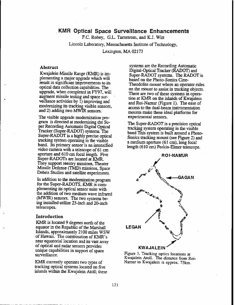
KMR Optical Space Surveillance Enhancements F.C. Robey, G.L. Tarnstrom, and K.J. Witt

Lincoln Laboratory, Massachusetts Institute of Technology,

Lexington, MA 02173

Abstract Kwajalein Missile Range (KMR) is implementing a major upgrade which will result in significant improvements to its optical data collection capabilities. The upgrade, when completed in FY97, will augment missile testing and space surveillance activities by 1) improving and modernizing its tracking visible sensors, and 2) adding two MWIR sensors.

The visible upgrade modernization program is directed at modernizing the Su- per Recording Automatic Digital Optical Tracker (Super-RADOT) systems. The Super-RADOT is a highly precise optical tracking system operating in the visible band. Its primary sensor is an intensified video camera with a telescope of 61 cm aperture and 610 cm focal length. Five Super-RADOTs are located at KMR. They support reentry missions, Theater Missile Defense (TMD) missions, Space Debris Studies and satellite experiments.

In addition to the modernization program for the Super-RADOTS, KMR is com- plementing its optical sensor suite with the addition of two medium wave infrared (MWIR) sensors. The two systems being installed utilize 23-inch and 20-inch telescopes.

Introduction KMR is located 9 degrees north of the equator in the Republic of the Marshall Islands, approximately 2100 miles WSW of Hawaii. The combination of KMR's near equatorial location and its vast array of optical and radar sensors provides unique capabilities in support of space surveillance.

KMR currently operates two types of tracking optical systems located on five islands within the Kwajalein Atoll; these

systems are the Recording Automatic Digital-Optical Tracker (RADOT) and Super-RADOT systems. The RADOT is based on the Photo-Sonics Cine- Theodolite mount where an operator rides on the mount to assist in tracking objects. There are two of these systems in operation at KMR on the islands of Kwajalein and Roi-Namur (Figure 1). The ease of access to the dual-beam instrumentation mounts make these ideal platforms for experimental sensors.

The Super-RADOT is a precision optical tracking system operating in the visible band This system is built around a Photo- Sonics tracking mount (see Figure 2) and a medium aperture (61 cm), long focal length (610 cm) Perkin-Elmer telescope.

ROI-NAMUR

r <£

^ ^ GAGAN

V

LEGAN

\ fi

\

J V KWAJALEIN^

Figure 1. Tracking optics locations at Kwajalein Atoll. The distance from Roi- Namur to Kwajalein is approx. 75km.

121

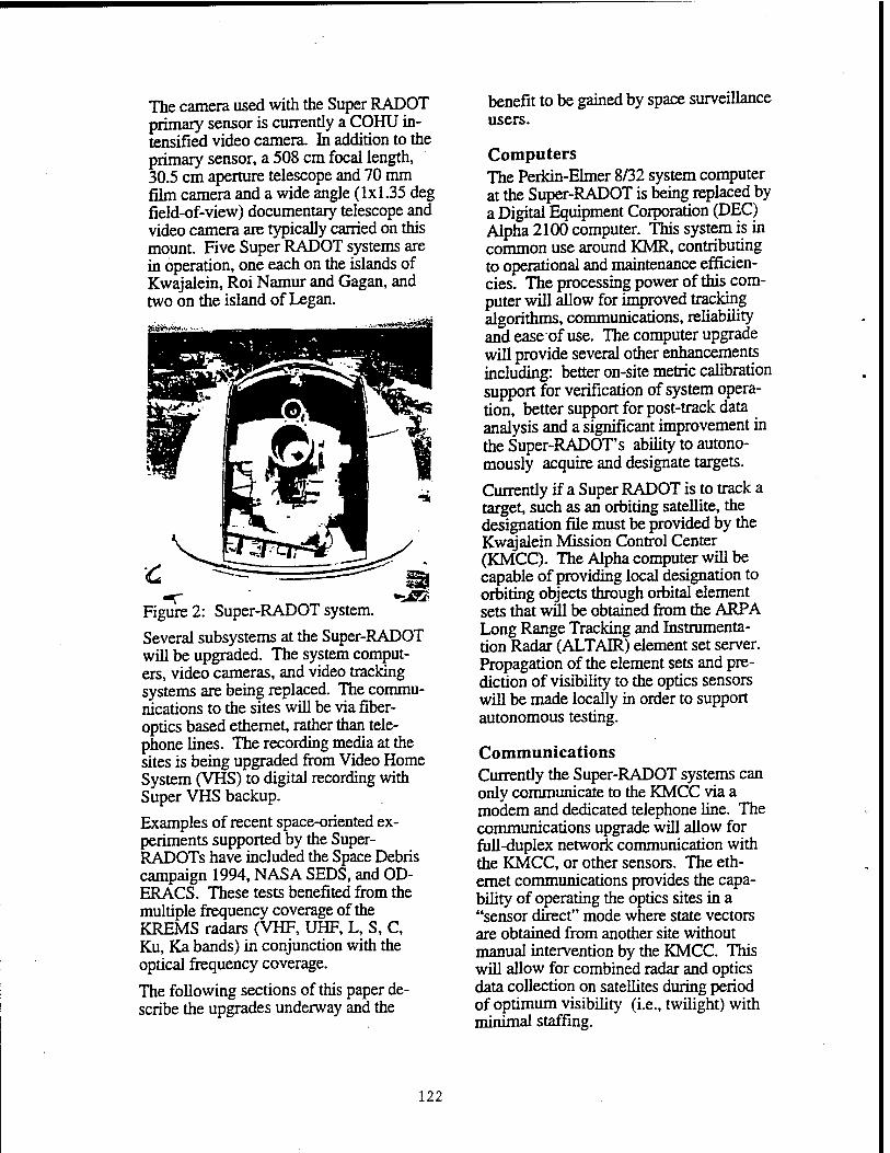
The camera used with the Super RADOT primary sensor is currently a COHU intensified video camera. In addition to the primary sensor, a 508 cm focal length, 30.5 cm aperture telescope and 70 mm film camera and a wide angle (1x1.35 deg field-of-view) documentary telescope and video camera are typically carried on this mount. Five Super RADOT systems are in operation, one each on the islands of Kwajalein, Roi Namur and Gagan, and two on the island of Legan.

«sdQ Figure 2: Super-RADOT system.

Several subsystems at the Super-RADOT will be upgraded. The system computers, video cameras, and video tracking systems are being replaced. The communications to the sites will be via fiber- optics based ethemet, rather than telephone lines. The recording media at the sites is being upgraded from Video Home System (VHS) to digital recording with Super VHS backup.

Examples of recent space-oriented experiments supported by the Super- RADOTs have included the Space Debris campaign 1994, NASA SEDS, and OD- ERACS. These tests benefited from the multiple frequency coverage of the KREMS radars (VHF, UHF, L, S, C, Ku, Ka bands) in conjunction with the optical frequency coverage.

The following sections of this paper describe the upgrades underway and the

benefit to be gained by space surveillance users.

Computers The Perkin-Elmer 8/32 system computer at the Super-RADOT is being replaced by a Digital Equipment Corporation (DEC) Alpha 2100 computer. This system is in common use around KMR, contributing to operational and maintenance efficien- cies. The processing power of this computer will allow for improved tracking algorithms, communications, reliability and ease of use. The computer upgrade will provide several other enhancements including: better on-site metric calibration support for verification of system operation, better support for post-track data analysis and a significant improvement in the Super-RADOT's ability to autono- mously acquire and designate targets.

Currently if a Super RADOT is to track a target, such as an orbiting satellite, the designation file must be provided by the Kwajalein Mission Control Center (KMCC). The Alpha computer will be capable of providing local designation to orbiting objects through orbital element sets that will be obtained from the ARPA Long Range Tracking and Instrumenta- tion Radar (ALTAIR) element set server. Propagation of the element sets and prediction of visibility to the optics sensors will be made locally in order to support autonomous testing.

Communications Currently the Super-RADOT systems can only communicate to the KMCC via a modem and dedicated telephone line. The communications upgrade will allow for full-duplex network communication with the KMCC, or other sensors. The ethemet communications provides the capability of operating the optics sites in a "sensor direct" mode where state vectors are obtained from another site without manual intervention by the KMCC. This will allow for combined radar and optics data collection on satellites during period of optimum visibility (i.e., twilight) with minimal staffing.

122

The additional bandwidth of the communication link will allow the direct transmission of digital data to KMCC and to the KMR Data Analysis Center (KDAC) in Lexington, Massachusetts. Rather than copying files to tape, hand-carrying the tapes and manually copying from the tape for transmission to KDAC, as is now the case, the files will be transmitted over the network to the KMCC where they are queued for transmission to KDAC via a high speed satellite link. This will allow data products such as digitally recorded video and intensity data to be made available to the user more quickly at lower costs.

Cameras After this upgrade is completed, there will be four cameras available for use with the main sensors at the optics sites. For any data collection, the specific camera will be determined by the users needs. The four cameras are described in this section.

The first camera is an anti-blooming charge coupled device (CCD) camera, primarily for use in reentry missions. The second camera is a Kodak high speed video camera. This camera was selected primarily for supporting TMD data collection and has the capability of digitally recording the video at 1000 frames per second. The imager is 512 by 384 pixels and the expected noise floor is the equivalent of 9th to 10th magnitude stars when operated at a 30 Hz frame rate. To increase the sensitivity, on-camera integration of up to 1 second is possible. For rapidly fluctuating objects this camera could be mated to an intensifier to increase the sensitivity.

The Xybion ISG-350 intensified CCD camera is available at KMR and has been tested for use with the Super RADOT. This camera features gating for short exposures as well as provisions for multi- frame integration on the imager chip (0.5 seconds, or 15 frames maximum). As with the current COHU cameras, the exposures of this camera are synchronized between sites. The noise floor expected with this camera is equivalent to 17th or

18th magnitude stars for a 33msec exposure.

The camera currently in use at the KMR Super RADOTs is the COHU Intensified. Silicon Intensifier Target (ISIT) video camera. This camera is ungated, but is time synchronized between sites. The measured noise floor of this camera is the equivalent of 17th to 18th magnitude stars.

These four cameras will provide the flexibility needed to support the TMD, reentry and space surveillance users of KMR. In particular, it is expected that the Xybion camera will be a good match with the space surveillance requirements.

Video Signal Processor A new video signal processor is being implemented for the Super-RADOT and other KMR video systems. This video signal processor is based on a Silicon Graphics Incorporated (SGI) Indy workstation. Two of" these workstations will be used with each Super RADOT system. The Indy workstations have been upgraded with enhanced video and real-time video compression cards. The ethernet interface of the Indy workstation will be used to provide communication to the Al- pha computer and to KMCC.

The processing power of the SGI computer allows implementing in software several functions that are currently implemented in hardware, are manually controlled, or are a post-mission operation. Control of video camera gain (intensifier high voltage) and telescope focus will be accomplished automatically with the workstation.

The video analysis capabilities of the Indy will be used to perform real time video target tracking and object centroiding. Video position measurements will be used to implement closed-loop object tracking and to enable mount metric calibrations. Background and object intensity measurements will be used to assist in photometry and signature measurements as well as to implement an automatic video gain control loop. For some

123

space surveillance users, the background and object intensity measurements along with calibration data may be sufficient data for their needs, removing the need to later analyze the video images.

The real time video compression card is being used to perform real-time digital video recording. Although the video digitization is only to 8 bits, the recording does not suffer from the degradation that is inherent in the VHS recordings, lead- ing to an improvement in overall system resolution and sensitivity.

In addition to the video analysis capabilities of the Indy workstation, this system . will also provide some operator's interface functions. Real time video in an X- window is provided with overlays and annotation surrounding the video display. A signature display, a mount position display and expected star calibrations displays are to be implemented.

Recording An analysis of the video system for the Super RADOTs shows that the VHS recording system currently in use limits the sensitivity and resolution. In order to alleviate this shortfall, the video will be digitally recorded by the video processing system, and a backup will be provided by Super-VHS recorders. The Super-VHS recorders provide negligible increase in dynamic range, but provide a dramatic increase in resolution.

MWIR Systems

Two mid-wave (3-5 (x) infrared (MWIR) systems are currently being integrated by KMR. MWIR has the advantage over the visible wavelengths in that the sky brightness is much less in this band, and there is less degradation of the signal by the atmosphere.

The two systems to be installed at KMR are a 23-inch telescope, previously located at the now-closed Army Optical Site on Roi-Namur, and a new 20-inch F3 telescope. The camera to be used with the latter is an Amber Galileo camera which features up to an 120 Hz full-frame

rate. This system has a low operational cost based on the built-in calibration and lack of need for liquid nitrogen. These two systems are being assembled primarily for TMD users, but will provide capabilities that may be of interest to space surveillance users.

Calibration The current system computers contain the algorithms and data needed to designate the mount to stellar sources for metric calibration. The new system computers will allow for photo-metric calibration as well. It is planned that the system computer analyze the trajectory and designate the mount to stellar photometric calibration sources immediately after tracking an object. Analysis of the object and calibration source intensities by the Indy and knowledge of the gain settings will provide calibration coefficients that will be stored for later correction of the data.

Conclusion Significant improvements are underway at KMR which will enhance the capabilities of the existing visible optics tracking sensor suite. These improvements are also being augmented by the addition of two MWIR sensors. A summary of the improvements in the systems and operation is shown in the Appendix.

KMR is a unique among test ranges in that it can provide simultaneous collection of both signature and metric data at multiple frequencies (VHF, UHF, L-Band, S-band, C-band, Ku, Ka, MWIR and visible).

Although these upgrades are not specifically aimed at the space surveillance users, the upgrades will significantly enhance KMR's capabilities to better support space surveillance data collection.

124

Appendix A comparison of system features

Table 1 lists the differences in the overall Super RADOT system features between the current and the upgraded systems. Table 2 illustrates the main camera features, and Table 3 shows the performance expected from the new MWIR systems. Table 1, Super RADOT system differences.

Previous New

Computer Technology Perkin-Elmer 8/32 DEC AXP-2100

Acquisition source radar radar or doc. camera

Tracking filter quadratic Kaiman or polynomial

Metric Calibration manual+ off-island processing

automatic + local processing

Communication half duplex @9600 baud from the control center

full duplex ethernet with other networked sensors and the control center

Table S >, Super RADOT main camera differences.

Previous New

COHU ISIT

Kodak 1000HR

Pulnix 745E

Xybion ISG-350

Focal plane technology

Intensified tube

CCD CCD Intensified CCD

Noise floor @30Hz (equiv mag)

17 10 7 17

Resolution (lp- |irad)

3.4 3.4 1.7 2.7

Frame/field Rate (Hz)

30/60 <1-1000 30/60 30/60

Integration time 16ms 20[is -> Is 32u.s ->ls 100ns->0.5s other variable focal

plane distortion and offset due

to magnetic fields

125

Table 3, Expected MWIR system performance

SSG AOS

Telescope Aperture (m) 0.51 0.58

Focal Ratio 3 2.4

Camera Amber Galileo Amber Radiance 1

Camera Technology InSb InSb

Array 256x256 256x256

Filter (um) 3.5 - 4.1 3.0 - 5.0

IFOV Oir) 20 27

Full Frame Rate (Hz) 60 - 120 60

Partial Frame Rate (Hz) 240 - 1400 n/a

Integration Time 2 us-16 ms 0-16ms

Recording S-VHS, 8 or 12 bit digital, or partially reduced data

Sterling cooling

2-point calibration

126

Satellite Tracking Using the TOTS

N.W. Heys & P.F. Easthope (Advanced System Architectures Ltd.)

1 INTRODUCTION

TOTS is a generic, multi-sensor, multi-target, fusion and tracking system, developed under a cooperative agreement between DOD BMDO and MOD DSc (BMD). TOTS employs a concurrent architecture, incorporating a bank of Kaiman filters, each using a different dynamic model.

As part of the proving trials, the system was installed at the White Sands Missile Range to test its operation in a real-time multi-sensor environment, with a range of typical targets. One of the experiments carried out was to track high quality satellite 'truth' data. It was observed that while TOTS produced a good track throughout the satellite pass, there was some divergence in the ballistic model. Subsequent analysis has determined that this is because the TOTS ballistic model neglects terms beyond the J2 gravitational harmonic in the WGS-84 earth model. This paper presents the analysis of the effect of neglecting these higher order terms, and in addition considers the perturbation of the orbit due to the sun and moon.

The analysis examines methods to modify the TOTS ballistic filter to mitigate against this effect without significantly increasing the computational resources needed to execute the algorithm. This has resulted in the addition of a small amount of extra process noise by two different techniques. Results from TOTS, using the modified filter, shows that the LEO satellite is tracked to a precision of better than 1 metre; without the extra process noise, the track diverges. Both techniques appear equally good, further test data sets are needed to see whether one has advantages over the other.

The paper also looks at the effect of other exo-atmospheric perturbations such as lunar/solar gravitational forces, solar pressure, etc., and demonstrates that the chosen solution can also cope with these effects.

2 TRACKING THE TRUTH DATA

The data set that originally exposed the potential ballistic model track divergence related to the LEO satellite. It contains the satellite trajectory 'truth' locations, formed from a composite of known orbital parameters and accurate sensor measurements. For TOTS tracking purposes, the state vectors (positions and velocities) are represented in 'pseudo-sensor' format, with the state vectors converted to range and bearing data relative to the sensor, which are then input to TOTS. The sensor was assumed to be a radar positioned on the earth's surface at latitude 32 deg. N and longitude 106 deg. W. This places it in the vicinity of the WSMR. Initially the sensor uncertainties were taken as 10 m. in range and 0.1 mrad. in angle. The ballistic model in this case contained gravitational terms up to J2. The tracking performance in position and velocity is shown in Figures 1 and 2 together with TOTS' prediction of its tracking accuracy. It can be seen that the tracking error increases sharply towards the end of the scenario, particularly after the uncertainty becomes

127

14

12 -

10

e -

56400 56500 56600 56700 56800 56900 57000 57100 57200 57300 57400 57500 Scenario Time (Seconds)

Figure 1: Position Tracking Error including Various J terms

smaller than the error.

It was thought that the reason could be that the ballistic model used to track the data was not accurate enough. However, the frequent update rate, (20 Hz.), should pull the track back onto the data. The J3 and J4 gravitational terms were therefore added to the ballistic model. The tracking performance is also shown in Figures 1 and 2. It can be seen that the additional terms give a slight improvement, particularly towards the end of the scenario. The J5 and J6 terms made little difference.

Further investigation showed that the process noise in the ballistic model is extremely small owing to the 50 ms. interval between "sensor readings". This means that the TOTS is very confident its prediction is correct, causing it to place little weight on the sensor data, resulting in the divergence. This implies that there are some aspects of the orbit which are not accurately described by the inclusion of gravitational terms up to J6. These could include the longitude dependence of the gravitational potential, which can be described by further harmonics and the effect of solar and lunar gravitational fields. Instead of going to the complexity of trying to model all these other terms, it is possible to account for them by increasing the process noise in the Kaiman Filter. Two different methods of achieving this are examined in the following sections.

3 THE USE OF FITZGERALD NOISE

Fitzgerald [1] suggested increasing the size of the diagonal velocity terms of the process noise covariance matrix to compensate for these unknown errors. A value of 10_5m2s-2 was tried.

The improvement in the tracking performance is shown in Figures 3 and 4, where the additional noise prevents the divergence from the "sensor data".

128

0.O45

0.04

0.03S

0.03

0.025

0.02

0.015

0.01

0.005

56400 56500 566OO 56700 56800 56QOO 57000 571OO 57200 57300 57400 57500 Scenario Time (Seconds)

Figure 2: Velocity Tracking Error including Various J terms

12

10

g LU

J3& J4

Fitz 0.00001

56400 565O0 56600 5670O 56800 56900 57000 571OO 57200 57300 57400 57500 Scenario Time (Seconds)

Figure 3: Position Tracking Error with and without 0.00001 Fitzgerald Noise

129

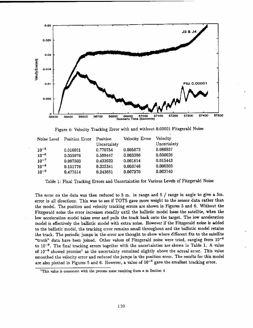
0.03

0.025

0.02

LU 0.015

o O

5 0.01

0.005

-l r

56400 56500 56600 56700 56800 56900 57000 57100 57200 57300 57400 57500 Scenario Time (Seconds)

Figure 4: Velocity Tracking Error with and without 0.00001 Fitzgerald Noise

Noise Level Position Error Position Uncertainty

Velocity Error Velocity Uncertainty

IO"5 0.016021 0.770754 0.005872 0.086857 10~6 0.055976 0.588447 0.003386 0.036626 io-7 0.097503 0.433932 0.001814 0.015443 io-8 0.151776 0.325341 0.003746 0.006509 IO"9 0.477514 0.243651 0.007370 0.002740

Table 1: Final Tracking Errors and Uncertainties for Various Levels of Fitzgerald Noise

The error on the data was then reduced to 5 m. in range and 5 / range in angle to give a 5m. error in all directions. This was to see if TOTS gave more weight to the sensor data rather than the model. The position and velocity tracking errors are shown in Figures 5 and 6. Without the Fitzgerald noise the error increases steadily until the ballistic model loses the satellite, when the low acceleration model takes over and pulls the track back onto the target. The low acceleration model is effectively the ballistic model with extra noise. However if the Fitzgerald noise is added to the ballistic model, the tracking error remains small throughout and the ballistic model retains the track. The periodic jumps in the error are thought to show where different fits to the satellite "truth" data have been joined. Other values of Fitzgerald noise were tried, ranging from 10~6

to IO"9. The final tracking errors together with the uncertainties are shown in Table 1. A value of IO-8 showed promise1 as the uncertainty remained slightly above the actual error. This value smoothed the velocity error and reduced the jumps in the position error. The results for this model are also plotted in Figures 5 and 6. However, a value of 10~5 gave the smallest tracking error.

'This value is consistent with the process noise resulting from K in Section 4

130

UJ

g

i

2.5

1.5

0.5

s / J3 & J4

/' /

/

/

/:.. <*■■

r^T— _?wJWJW _iu. JW _iw. ,-iW JU. JUT JU.~:R^ . TU/y

Fitz 1 .Oe-8

^FjtzO.OQOpi 56400 56500 5O600 567O0 56800 56000 57000 57100 57200 57300 57400 57500

Scenario Time (Seconds)

Figure 5: Position Tracking Error with Smaller Measurement Error and Different Noise

0.07

v - -■■ —- *" ■

56400 5650O 56600 5670O 56800 56000 57000 571OO 57200 57300 57400 57SOO Scenario Time (Seconds)

Figure 6: Velocity Tracking Error with Smaller Measurement Error and Different Noise

131

4 NUMERICAL EXPERIMENTS USING MODIFIED PROCESS NOISE

The alternative method of modifying the process noise determines the relative size, n, (K « 3xl(M), of the neglected accelerations to the dominant ballistic acceleration term £. Additional noise, accounting for this term, is added to both the position and velocity elements of the process noise covariance matrix.

The data set used for the experiments is the same as that described in Section 2, although the uncertainties used were slightly different. The 'truth' satellite positions are believed accurate to 5 m., so in this case, the synthetic sensor was assigned a range uncertainty of 5 m. and an angular uncertainty of 5 /zrad. (based on the minimum sensor-target distance of 106 m.; the maximum such distance is about 3 x 106 m.).

The assessment of tracking performance on this data set is here devolved to two quantities Xt and

Xu, where:

X« =

/As2 + Ay2 + A*2

■*arr i~ -^"Vy "i •*.zz

\Av? + At;2 + Am2

The Ax, etc., quantities are components in the vector difference of track and 'truth', and the Pxx, etc., are the diagonal components of the track error covariance matrix.

For a statistically consistent tracking filter, it is expected that both x« and Xt« have mean values of unity.

Looking first at the case of basic ballistic tracking model, with no compensation for missing gravitational harmonics, the ensuing statistical measures are plotted in Figure 7. It can be seen that the track is diverging, particularly in velocity.

Figure 8 shows the equivalent statistical measures for the case when the quantity K is accounted for in the process noise; here, the tracking performance is entirely satisfactory.

Equivalent comparisons using simulated data, in which the trajectory was generated with harmonic terms up to 78, have shown little difference between including K or excluding it from the process noise. In the simulated data, however, the update interval is 1 s., whereas for the LEO satellite data, it is 50 ms., and in the latter case the small update interval causes the basic process noise resulting from discretisation to become very small also.

132

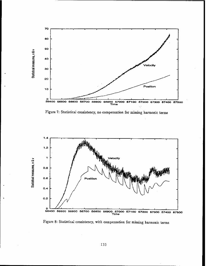
>• öS

of

CO

70

SO

50

40

30

20 -

10 -

S6400 56500 56600 56700 56800 S6900 57000 571OO 57200 S7300 57400 S7600 Time

Figure 7: Statistical consistency, no compensation for missing harmonic terms

s 1 co

1.4

1.2

0.8 -

0.6 -

0.4

0.2

56400 56500 56600 56700 S6SOO 56900 67000 571OO 67200 67300 67400 57600 Time

Figure 8: Statistical consistency, with compensation for missing harmonic terms

133

5 SOLAR, LUNAR AND PLANETARY PERTURBATIONS

One possible source of inaccuracy in the equations representing the orbit is the effect of the gravitational fields of the sun, moon and planets on the orbit. Including these terms but omitting the earth oblateness terms, the equation of motion of a ballistic body can be written ([2]):

R3 x 2>*M,r.#|3 |ri„

where the centre of the earth is taken as origin, the suffix e refers to the earth and the suffix s refers to the missile or satellite. G is the gravitational constant, and R = |x|. The summation is over all the planets, mass Mj, plus sun and moon, but excluding the earth. For brevity, the earth's gravitational field is simplified here.

The vectors r,-, and r,e are defined as:

Tja = r4 - TJ for perturbing body j,

= x-rj,

rje = re-rj

= —Tj due to the choice of coordinate origin.

Thus,

i?3 £, J\Jrj|3 Ix-Tjf

Since m3 < Afe, and |x| < jr-j-j for all j (assuming that the satellite is in relatively close proximity to the earth). The quantity |x - Tj\3 can then be approximated, with the result:

GMe ^ GMj ( x~ &x fzwK* k,f T')+0\ GMj

where Rj = jr^-j.

From this equation, the perturbation effects in the second term on the right-hand-side will have a maximum value of order

2GMjR R)

The following values can then be used for the sun and moon (those of dominant effect):

134

MJJM Rj ("*•) Sun Moon

1.99 x 1Ö35" 7.349 x 1020

1.496 x 10u

3.844 X 108

When only the sun and moon are considered the acceleration:

x = -Ms ■"-je.

-Mn X-mb

ßmb (1)

where /x is the gravitational parameter, x is the position vector, R is the distance from one body to another, Subscript s denotes the sun, Subscript e denotes the earth, Subscript m denotes the moon,

and Subscript b denotes the satellite

The equation of motion of the satellite therefore requires the position vector of the sun relative the earth and satellite and the position vector of the moon relative to the earth and satellite. These will not be readily known, so it is not practical to include the effect of the sun and moon directly in the equations of motion. However, the relative size of the accelerations compared to those produced by the earth can be determined.

In order to calculate the net effect of the sun and moon on the satellite after subtracting the effect on the earth's orbit, the following gravitational parameters are needed for the sun and moon, respectively:

3 „-2 fj.a = GMS = 1.32733 x 1020m3s

ßm = GMm = 4.901783 x 10lomV

where G = 6.673 x 10~n Nm2kg~2 is the gravitational force.

Calculating the sizes of the full sun and moon terms in (1) and dividing by g, gives values of the sun and moon accelerations which are given in Table 2 and compared with the earth terms for a satellite in a 200 nautical mile orbit about the earth. The effect of the planets is much smaller than the sun and moon. For a satellite at 800 km. altitude (a typical altitude for the LEO satellite data), R ~ 7178137 m., and the following perturbation values obtain:

_2 ms g Sun Moon

5.69 X 10"7

1.24 x 10"8 7.35 X 10"8

1.6 x 10"9

where V is 7.736 ms 2 (the acceleration due to the earth's gravitational field at this altitude).

It is clear that the solar, lunar and planetary effects are negligible compared to the neglected earth harmonics and can also be neglected.

135

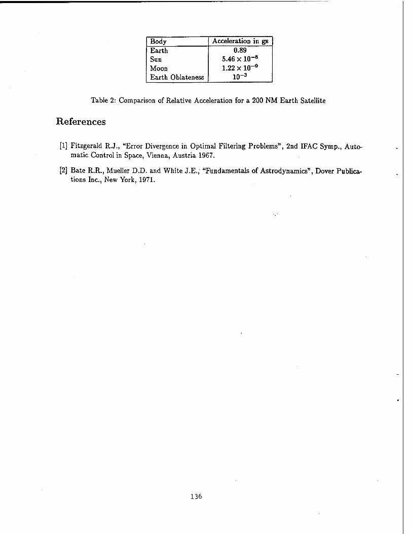
Body Acceleration in gs Earth 0.89 Sun 5.46 X 10-8

Moon 1.22 x It)-9

Earth Oblateness 10"3

Table 2: Comparison of Relative Acceleration for a 200 NM Earth Satellite

References

[1] Fitzgerald R.J., "Error Divergence in Optimal Filtering Problems", 2nd IFAC Symp., Auto- matic Control in Space, Vienna, Austria 1967.

[2] Bate R.R., Mueller D.D. and White J.E.; "Fundamentals of Astrodynamics", Dover Publica- tions Inc., New York, 1971.

136

Earth Gravitational Error Budget for Space Control

R. N. Wallner, W. N. Barker, S. J. Casali, T. L. Yeiter (Kaman Sciences Corporation)

ABSTRACT

The primary objective of this study was to estimate a geopotential model error budget for a wide range of mission-essential orbits for the Space Defense Operations Center (SPADOC) space surveillance mission, in which it is necessary to maintain the orbits of many satellites using relatively noisy skin-track radar data. To achieve this goal, simulations that isolated purely geopotential effects were first conducted; and then actual data and realistic force models were used in an operational context to provide error assessments for orbit determination and prediction. The end result was a set of broad guidelines for geopotential truncation appropriate for the SPADOC mission. The geopotential models considered were World Geodetic System 1972 (WGS-72), WGS-84, and the NASA Joint Gravity Model 2 (JGM2).

INTRODUCTION

Due to the demand for very high positional accuracy in certain space operations, geopotential models have become increasingly more sophisticated and computationally intensive. However, there still exist many space applications in which the accuracy afforded by these models is neither required nor attainable (for non-geopotential related reasons). For these applications, large, wasteful computational burdens will be incurred unless the standard geopotential models are appropriately truncated. For applications involving a small number of satellites, this tailoring is usually straight-forward, but establishing general guidelines for a large number of satellites is more difficult.

The primary objective of this study was to estimate a geopotential model error budget for a wide range of mission- essential orbits for the Space Defense Operations Center (SPADOC) space surveillance mission. In this mission, it is necessary to use special perturbations methods to maintain the orbits of many satellites (potentially 500-1000) using relatively noisy Space Surveillance Network (SSN) skin-track radar data. In meeting this objective, the study also produced results applicable to space missions that process higher quality observations and have higher precision requirements. Also, the study briefly addresses the question of whether there exists a need for continued research of more sophisticated geopotential models for the space surveillance mission.

To accomplish the objective, a broad range of representative orbits were analyzed using two main techniques. First, simulations that isolated purely geopotential effects were conducted; and second, actual SSN data and realistic force models were used in an operational context to provide error assessments for orbit determination and prediction. Both methods were used to determine in a broad sense, for wide classes of orbits, the truncation level above which more geopotential yields no noticeable benefit for the SPADOC mission. The geopotential models considered were World Geodetic System 1972 (WGS-72), WGS-84, and the NASA Joint Gravity Model 2 (JGM2). The JGM2 model, one of the newest available, is of degree and order 70. The WGS-72 model, which is currently the primary model used by the SPADOC, is a 28x27 degree and order model. The WGS-84 model, which is used by the SPADOC for some missions, is of degree and order 180, of which we considered only the 70x70 portion.

Finally, in planning the study, a literature search pertaining to geopotential was conducted. Of the approximately 50 articles and books reviewed, a large portion was devoted to the details of the development and calibration of various gravity models. Further, a significant portion addressed the accuracies of various full model geopotentials for a few geodetically useful satellites (e.g., LAGEOS, ERS-1 and TOPEX) in the context of sub-meter positioning. None were particularly tailored toward the SPADOC space surveillance mission, and the literature that did pertain to an exhaustive number of orbits was analytical in nature. An example is Theory of Satellite Geodesy, by William Kaula , which provided insight into the design of meaningful test cases. As discussed later, other useful information from the search pertained to how much geopotential is required for certain "deep-space" satellites, which are defined by the SPADOC as having a period greater than 225 minutes. In summary, though, no studies were found that could be used directly for comparison to our study.

137

STUDY DATA AND SOFTWARE

The data used for the study included all the SPADOC Verified Observations as well as daily SPADOC element sets on 49 test satellites over the period October 1993 to June 1994. These 49 satellites were comprised of seven satellites in each of seven orbit categories. These categories, described in Table 1, were defined so as to distinguish broad regions in which different perturbative effects are dominant while keeping the number of categories reasonable. Table 1 shows that the large majority of satellites currently in orbit are represented.

Table 1 ORBIT CATEGORIES

Category Number

Name Eccentricity Mean Altitude (km)

Number in Catalog*

%of Catalog*

I Low Near Earth Circular

•0.0 < e < 0.05 0< fc<575 166 2.45

2 Medium Near Earth Circular

0.0 < e < 0.05 575 < h < 1000 2460 36.36

3 High Near Earth Circular

0.0 < e < 0.05 1000 < h < 2500 2014 29.77

4 Near Earth Eccentric

0.05 <e< 1.0 0 < h < 2500 652 9.64

5 Low Deep Space Circular

0.0 < e < 0.05 5700 < h < 22000 115 1.70

6 Molniya/ Geosynchronous

Transfer

0.05 <e< 1.0 18000 < h < 22000 403 5.96

7 Geosynchronous 0.0 < e < 0.05 33000 < h < 39000 480 7.09

TOTAL 6290 92.96

The primary analysis tool used was Kaman Sciences Corporation's special perturbations differential correction and prediction program SPECTR (Satellite Propagation and Element Correction for Test and Research), which is numerically compatible with the SPADOC. SPECTR uses an 8th-order Gauss-Jackson predictor-corrector numerical integrator and models perturbations due to geopotential (up to degree and order 70), atmospheric drag, lunar-solar gravity, direct solar radiation pressure, and constant in-track thrust. For differential corrections, standard weighted (or, optionally, unweighted) least-squares batch estimation is employed.

INTEGRATOR STEP SIZE DETERMINATION

Before beginning the study, it was necessary to develop a new integrator step size selection algorithm, because the existing one was tailored toward low degree and order (12 or less) geopotentials, and using it could incur numerical integration errors that might invalidate our results. In order to do this, many trials were performed, decreasing the step size each time, until the ephemeris difference between a run using a particular step size and a run using one-half the step size was less than one meter over one week. This process was repeated for many different orbit types, and an algorithm was developed. The new algorithm is as follows:

For altitudes between 100 km and 720 km, the initial integration step size should be:

We defined mean altitude as the semi-major axis minus the Earth's equatorial radius. As of August 31, 1993.

138

S= 77^ + 50 (steps/rev) (1)

where T is the truncation degree, and K is a non-linear function of the mean motion (n) in revs/day:

K = 0.50853>22-14.2502/2 + 100.413 (2)

Below 100 km, an empirically determined step size of 0.1875 minutes was adopted. Above 720 km, 100 steps/rev was found to be appropriate.

SENSITIVITY STUDY

A satellite trajectory that results from using a truncated geopotential model obviously contains a certain amount of mis-modeling relative to a trajectory that uses the full model. This phase of the study attempted to isolate and quantify this mis-modeling by conducting simulations that considered only geopotential perturbations, with emphasis placed on errors with short-periodic and daily frequencies. These errors were given the attention because they represent a level of "noise" that is always present in an operationally performed orbit determination (OD). In all, 57 simulated orbits were chosen in order to adequately sample the geopotential and span the Kaman orbit categories.

Due to space limitations, the details of the sensitivity study methodology and results have been omitted. In general, the results agreed well with the results of the Orbit Determination and Prediction Accuracy Study (discussed below). A complete discussion of the sensitivity study is available upon request.

ORBIT DETERMINATION AND PREDICTION ACCURACY STUDY

The objective of this phase of the study was to determine the geopotential error budget under SPADOC operational conditions. In this phase, actual SSN observational data was used, and all major perturbative effects were modeled in conjunction with geopotential. The methodology that was used was based upon the methodology used by Barker2: For each satellite, geopotential model, and truncation degree/order, we solved for a state vector using actual SSN observations at many different times, used the output state vector to predict the satellite's position into the future, and compared the predictions to future observations. The details of this methodology are given below. For this study, we analyzed two satellites per Kaman orbit category, as shown in Table 2.

SAT Table 2

ELLITES STUDIED Orbit

Category Satellite

# Name Period

(min) Inclination

(deg) Apogee

(km) Perigee

(km) LUPI' (days)

1 12071 Cosmos 1222 95.9 81.2 563 557 7 1 20496 USA 51 94.1 43.1 483 465 6 2 7646 Starlette 104.2 49.8 1107 806 10 2 15427 NOAA9 101.8 99.1 854 833 10 3 50 Echo 1 R/B 118.1 47.2 1684 1502 14 3 671 5E1 107.1 90.0 1123 1062 13 4 12 Vanguard 2 R/B 127.1 32.9 3433 558 8 4 3530 Cosmos 252 112.0 62.3 2110 528 7 5 8820 Lageos 225.4 109.9 5945 5837 14 5 20724 USA 63 718.0 54.7 20468 19895 25 6 22068 Molniya 3-43 717.7 63.0 39327 1025 25 6 22255 Molniya 1-84 717.7 63.2 39997 351 17 7 7318 ATS 6 1412.1 12.9 35449 35179 25 7 10516 Sakura 1A 1455.8 10.2 36184 36159 25

The LUPI algorithm is a function of perigee altitude and eccentricity, and is optimized to give good results in prediction.

139

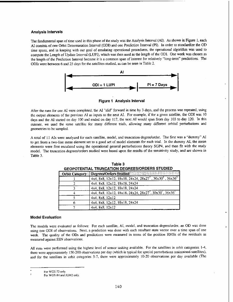
Analysis Intervals

The fundamental span of time used in this phase of the study was the Analysis Interval (AI). As shown in Figure 1, each AI consists of one Orbit Determination Interval (ODI) and one Prediction Interval (PI). In order to standardize the OD time spans, and in keeping with our goal of emulating operational procedures, the operational algorithm was used to compute the Length of Update Interval (LUPI), which was then used as the length of the ODI. One week was chosen as the length of the Prediction Interval because it is a common span of interest for relatively "long-term" predictions. The ODIs were between 6 and 25 days for the satellites studied, as can be seen in Table 2.

Al

ODI = 1 LUPI PI = 7 Days

Figure 1 Analysis Interval

After the runs for one AI were completed, the AI "slid" forward in time by 3 days, and the process was repeated, using the output elements of the previous AI as inputs to the next AI. For example, if for a given satellite, the ODI was 10 days and the AI started on day 100 and ended on day 117, the next AI would span from day 103 to day 120. In this manner, we used the same satellite for many different trials, allowing many different orbital perturbations and geometries to be sampled.

A total of 11 Als were analyzed for each satellite, model, and truncation degree/order. The first was a "dummy" AI to get from a two-line mean element set to a good set of model elements for each trial. In the dummy AI, the mean elements were first osculated using the operational general perturbations theory SGP4, and then fit with the study model. The truncation degrees/orders studied were based upon the results of the sensitivity study, and are shown in Table 3.

Table 3 GEOPOTENTIAL TRUNCATION DEGREES/ORDERS STUDIED

Orbit Category Degrees/Orders Studied 1 4x4, 8x8, 12x12, 18x18, 24x24, 28x27*, 30x30+, 36x36+

2 4x4,8x8, 12x12,18x18,24x24 3 4x4,8x8, 12x12, 18x18,24x24 4 4x4, 8x8, 12x12, 18x18, 24x24, 28x27*, 30x30f, 36x36T

5 4x4, 8x8, 12x12 6 4x4,8x8, 12x12, 18x18,24x24 7 4x4, 8x8, 12x12

Model Evaluation

The models were evaluated as follows: For each satellite, AI, model, and truncation degree/order, an OD was done using one ODI of observations. Next, a prediction was done with each resultant state vector over a time span of one week. The quality of the ODs and predictions were measured in terms of the position RMSs of the residuals as measured against SSN observations.

All runs were performed using the highest level of sensor tasking available. For the satellites in orbit categories 1-4, there were approximately 150-200 observations per day (which is typical for special perturbations maintained satellites), and for the satellites in orbit categories 5-7, there were approximately 10-20 observations per day available (The

For WGS-72 only. For WGS-84 and JGM2 only.

140

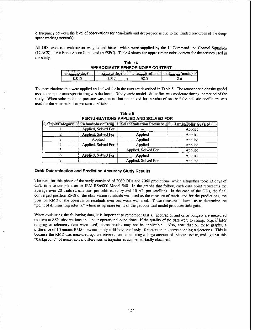
discrepancy between the level of observations for near-Earth and deep-space is due to the limited resources of the deep- space tracking network).

All ODs were run with sensor weights and biases, which were supplied by the 1st Command and Control Squadron (1CACS) of Air Force Space Command (AFSPC). Table 4 shows the approximate noise content for the sensors used in the study.

Table 4 APPROXIMATE SENSOR NOISE CONTENT

a^muftCdeg) Operation («kg) Cwe(m) oraiwerflte{m/sec) 0.018 0.017 38.5 2.6

The perturbations that were applied and solved for in the runs are described in Table 5. The atmospheric density model used to compute atmospheric drag was the Jacchia 70 dynamic model. Solar flux was moderate during the period of the study. When solar radiation pressure was applied but not solved for, a value of one-half the ballistic coefficient was used for the solar radiation pressure coefficient.

Table 5 PERTURBATIONS APPLIED AND SOLVED FOR

Orbit Category Atmospheric Drag Solar Radiation Pressure Lunar/Solar Gravity 1 Applied, Solved For — Applied 2 Applied, Solved For Applied Applied 3 Applied Applied Applied 4 Applied, Solved For Applied Applied 5 - Applied, Solved For Applied 6 Applied, Solved For Applied Applied 7 - Applied, Solved For Applied

Orbit Determination and Prediction Accuracy Study Results

The runs for this phase of the study consisted of 2060 ODs and 2060 predictions, which altogether took 13 days of CPU time to complete on an IBM RS/6000 Model 540. In the graphs that follow, each data point represents the average over 20 trials (2 satellites per orbit category and 10 Als per satellite). In the case of the ODs, the final converged position RMS of the observation residuals was used as the measure of merit, and for the predictions, the position RMS of the observation residuals over one week was used. These measures allowed us to determine the "point of diminishing returns," where using more terms of the geopotential model produces little gain.

When evaluating the following data, it is important to remember that all accuracies and error budgets are measured relative to SSN observations and under operational conditions. If the quality of the data were to change (e.g. if laser ranging or telemetry data were used), these results may not be applicable. Also, note that on these graphs, a difference of 10 meters RMS does not imply a difference of only 10 meters in the corresponding trajectories. This is because the RMS was measured against observations containing a large amount of inherent noise, and against this "background" of noise, actual differences in trajectories can be markedly obscured.

141

8.00 -

1 7.00- : -*-

—Ar— WGS72

—■—WGS84

♦ JGM2

s <E 6.00 - c o

| 5.00- a. c o 4 00-

—i—i—i—i—i—i—i—i—i—i—i—i—>-

rA

u

£ 3.00

2.00 - —i—i—i—i—i

12 16 20 24 Truncation Degree/Order


32 36

Figure 2 OD and Prediction RMS for Orbit Category 1

Figure 2 shows the results for orbit category l. In terms of both OD and prediction accuracy, there was very little difference between the three models in this category, except for degrees/orders above 18x18 for WGS-72. This difference, which is also evident in the other orbit categories, is due to the fact that many of the terms above 18x18 are missing from the WGS-72 model.

For both the OD and one week prediction interval, there is a clear increase in accuracy between 12x12 and 18x18. For these satellites, whose mean motions are between 14.9 and 16.3 revolutions per day, geopotential terms of order 15 and 16 cause resonances. These resonance terms can have a significant effect upon both the satellite's trajectory and the accuracy of solved-for parameters (in particular, the mean motion (n) and the ballistic coefficient (B)), which have a large influence on prediction. For the OD interval, the accuracy continues to increase until 30x30, but for the one week prediction, there is clearly no accuracy gain above 18x18.

1.06

_ 104

J 1.02

% 1.00

c 0.98 o I °"96

£ 0.94 --

S 0.92 -- u. Q 0.90 -- O

0.88 --

0.86

§2.80


8 12 16 Truncation Degree/Order


For orbit category 2, which is shown in Figure 3, there is again very little separation between the models. In this category, the same trends that were identified in category 1 were again evident: the same significant changes occur between 12x12 and 18x18 (although in this category, the resonances are of order 14 and 15 because the satellites' mean motions are between 13.7 and 14.9 revs/day).

142

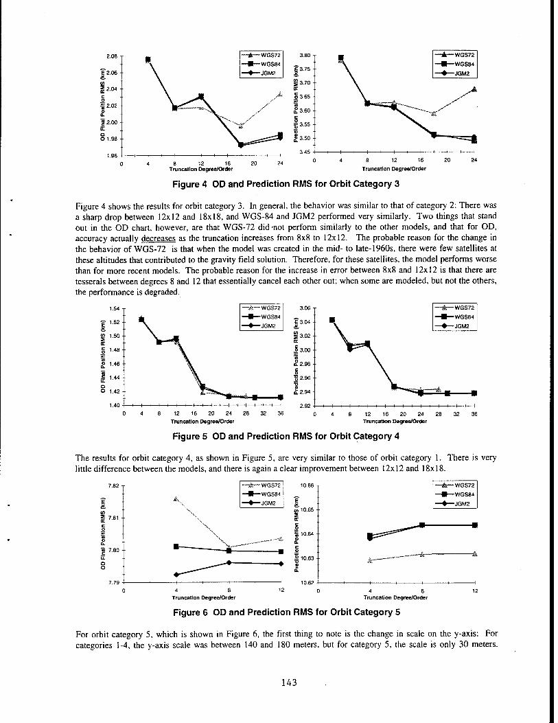
2.08 -

\ —T&—-WGS72

—•—WGS84

¥2.06 - —♦—JGM2

at f 2.04- c o = 2.02- o

OL

= 2.00 -

^\

u. ^L

o O 1.98 -

1.96 - 1 1 1 t- 1 ( H —i—i—i—i—i


3.80

r3.75

I 3.70

S3.65 9

13.60

) = 3.55 i •3.50

3.45 4-

0 8 12 16

Truncation Degree/Order

20 24


Figure 4 shows the results for orbit category 3. In general, the behavior was similar to that of category 2: There was a sharp drop between 12x12 and 18x18, and WGS-84 and JGM2 performed very similarly. Two things that stand out in the OD chart, however, are that WGS-72 did -not perform similarly to the other models, and that for OD, accuracy actually decreases as the truncation increases from 8x8 to 12x12. The probable reason for the change in the behavior of WGS-72 is that when the model was created in the mid- to late-1960s, there were few satellites at these altitudes that contributed to the gravity field solution. Therefore, for these satellites, the model performs worse than for more recent models. The probable reason for the increase in error between 8x8 and 12x12 is that there are tesserals between degrees 8 and 12 that essentially cancel each other out; when some are modeled, but not the others, the performance is degraded.

12 16 20 24 28

Truncation Degree/Order 12 16 20 24



The results for orbit category 4, as shown in Figure 5, are very similar to those of orbit category 1. There is very little difference between the models, and there is again a clear improvement between 12x12 and 18x18.

—jfe—WGS72

—■—WGS84

♦ JGM2

= 7.81

□ O

U> 10.65

£ 10.63 -

10.62

-WGS72

-WGS84

-JGM2

Truncation Degree/Order 4 8



For orbit category 5, which is shown in Figure 6, the first thing to note is the change in scale on the y-axis: For categories 1-4, the y-axis scale was between 140 and 180 meters, but for category 5, the scale is only 30 meters.

143

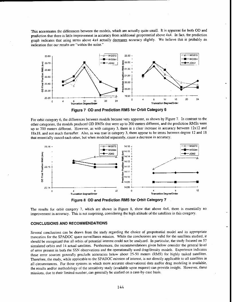
This accentuates the differences between the models, which are actually quite small. It is apparent for both OD and prediction that there is little improvement in accuracy from additional geopotential above 4x4. In fact, the prediction graph indicates that using terms above 4x4 actually decreases accuracy slightly. We believe this is probably an indication that our results are "within the noise."

J 22.00

c/> §21.50

§ 20.50

—A—WGS72

WGS84

JGM2

12 16 Truncation Degree/Order

8 12 16



For orbit category 6, the differences between models became very apparent, as shown by Figure 7. In contrast to the other categories, the models produced OD RMSs that were up to 200 meters different, and the prediction RMSs were up to 700 meters different. However, as with category 3, there is a clear increase in accuracy between 12x12 and 18x18, and not much thereafter. Also, as was true in category 3, there appear to be terms between degree 12 and 18 that essentially cancel each other, but when modeled separately, cause a decrease in accuracy.

= 23.15

23.14

-WGS72

-WGS84

-JGM2




The results for orbit category 7, which are shown in Figure 8, show that above 4x4, there is essentially no improvement in accuracy. This is not surprising, considering the high altitude of the satellites in this category.

CONCLUSIONS AND RECOMMENDATIONS

Several conclusions can be drawn from the study regarding the choice of geopotential model and its appropriate truncation for the SPADOC space surveillance mission. While the conclusions are valid for the satellites studied, it should be recognized that all orbits of potential interest could not be analyzed. In particular, the study focused on 57 simulated orbits and 14 actual satellites. Furthermore, the recommendations given below consider the general level of error present in both the SSN observations and the operationally used drag/density models. Experience indicates these error sources generally preclude accuracies below about 25-50 meters (RMS) for highly tasked satellites. Therefore, the study, while applicable to the SPADOC mission of interest, is not directly applicable to all satellites in all circumstances. For those systems in which more accurate observational data and/or drag modeling is available, the results and/or methodology of the sensitivity study (available upon request) can provide insight. However, these missions, due to their limited number, can generally be studied on a case-by-case basis.

144

First, it was found that the WGS-84 and JGM2 models performed very similarly in general. For the space surveillance mission, the WGS-84 model seems to be adequate, and therefore, a full SPADOC upgrade to WGS-84 is recommended because it is the DoD standard and is already implemented in the SPADOC. Not surprisingly, both the JGM2 and WGS-84 models generally proved superior to the older WGS-72 model. Ideally, of course, it would be desirable for the SPADOC to completely avoid using the older WGS-72 model, but compatibility with certain external users would be a problem were the SPADOC to use WGS-84 exclusively. It was also clear that both the WGS-84 and JGM2 models provide accuracies that are well within the accuracy limitations imposed by the SSN observations and the operationally used drag/density models. Not surprisingly then, the accuracy of the space surveillance mission will not be significantly improved by more sophisticated geopotential models.

Second, some broad geopotential truncation guidelines for the space surveillance mission are recommended in Table 6. Two sets of recommendations are presented. One is for "short-term" prediction, which here refers to predictions on the order of one day or less, while the other is for "long-term" prediction, which here refers to predictions on the order of one week. The short-term prediction recommendations are based on the results from the sensitivity study and on the OD results from the "real data" portion of the study, since if the prediction span is short enough, the prediction errors closely resemble the errors over the OD interval. On the other hand, the long-term prediction results are based on the one week predictions performed during the real data portion of the study. The distinction was made between short-term and long-term prediction because small errors in non-conservative model parameters can dominate the error growth over time, thereby negating some of the benefit provided by higher-order gravity modeling. In regard to the short-term prediction results, the sensitivity study and the real data portion of the study were generally in agreement as to when the point of diminishing returns was reached if the "noise cut-off is taken to be 25-50 meters (RMS) in the sensitivity study.

Table 6 RECOMMENDED TRUNCATIONS

Orbit Category Truncation (Short-term prediction)

Truncation (Long-term prediction)

1 (Above 450 km)

24-30 18

2 24 18 3 18 18 4 24 18 5 4 4 6 18 18 7 4 4

No conclusive recommendations can be made for satellites with altitudes below 450 km because no actual satellite data was readily available in this regime; however, the results of the sensitivity study indicate that anywhere from a 24x24 to a 36x36 model is required, depending on the altitude. Furthermore, for satellites with altitudes below about 1500 km, the often used 12x12 truncation generally does not provide all the accuracy obtainable from the SSN observations because it does not model certain resonances, as discussed in the results sections of both phases of the study. However, the study did not analyze the operationally used model for the Defense Meteorological Support Program (DMSP) satellites. This model uses a 12x12 base geopotential and includes resonance terms (the 14,14 and 15,14 terms) tailored specifically to the DMSP satellites. For this case, it is unclear whether a higher-order model will increase the accuracy significantly. Furthermore, for orbit category 6 (Molniya-like satellites), the recommended truncation level is clearly influenced by perigee altitude. For this category, perigee altitudes of approximately 350 km, 525 km (from the sensitivity study), and 1000 km were analyzed as a group. Orbit category 4 has a similar consideration; the orbits studied in this category had perigee altitudes ranging from 470 km to 560 km.

These recommendations were based entirely on accuracy considerations: we did not consider CPU usage in our truncation recommendations, even though all runs were CPU timed. There were two reasons CPU performance was not heavily considered: First, the recommended truncation levels were not unreasonably high compared to the ones commonly used in the SPADOC. Second, a detailed study on the trade-off between accuracy and CPU was beyond

145

the scope of this study, as it would have required a detailed analysis of the current day-to-day CPU allocations of the

SPADOC.

ACKNOWLEDGMENTS

This work was done under the direction of Dr. Joseph J. F. Liu of the Air Force Space Command Space Warfare Center (AFSPC/SWC) and Dr. Kitt C. Carlton-Wippern of the Air Force Materiel Command Space Systems Support Group (AFMC/SSSG), in support of contract F05603-91-C-0011. We are grateful to Drs. Liu and Wippern for

supporting this effort.

The authors would like to acknowledge the contributions of the following people: Tobey L. Yeiter, who performed a significant amount of work on this study; Ralph G. Schinnerer and Dr. Thomas J. Eller, for their guidance and comments; and Todd W. Bunker, Michele M. Kubis and Denis F. Durand, who assisted with the major modifications to SPECTR for this study.

REFERENCES

1. Kaula, W., Theory of Satellite Geodesy. Blaisdell: Waltham, Mass., 1966.

2. Barker, W. N., Casali, S. J., and Wallner, R. N., The Accuracy of General Perturbations and Semianalytic Satellite Ephemeris Theories. Presented at the 1995 AAS/AIAA Astrodynamics Specialist Conference (AAS 95- 432), Halifax, Nova Scotia, Canada, August 14-17, 1995.

146

DEEP SPACE IMAGING STUDY

Capt D. Rider (USAF Phillips Laboratory), C. Jingle, E. Nielson (W.J. Schäfer Associates)

ABSTRACT The USAF Phillips Laboratory is investigating methods for obtaining medium to high

resolution optical imagery of satellites in deep space orbits. Five concepts were evaluated for their ability to provide space object identification information on deep space satellites at low cost We report on the results of the Deep Space Imaging Study which documents our current understanding of the deep space problem relating to optical imagery and how the five imaging concepts considered address this problem. The results of the study led to the downselection of two concepts for further evaluation and a directed technical base program.

OBJECTIVE AND SCOPE What is the best way to image a deep space satellite? Obviously the answer depends on

how one defines "best". Best could mean with the highest resolution, at the lowest cost, with the least risk, or with the highest payoff for another, related, higher priority mission. Each of these factors is important and, as one might expect, no system is the best by all these definitions simultaneously. Nonetheless, the Deep Space Imaging Study (DSIS)1 attempts to answer this question or at least provide enough information to extract a reasoned decision based on a future, validated definition of best. The study presupposes that there is a need for optical imagery of deep space satellites. This general requirement has been validated and will not be discussed here. The study also presupposes a need for medium to high resolution imagery which may or may not be a validated requirement While all of the concepts have been evaluated on their ability to produce medium to high resolution imagery, this fact is not central to the conclusions we have reached in this report. In fact, the study team well understands that the "deep space problem" may be solved with low resolution imaging or even non-imaging methods.

The Deep Space Imaging Study is a culmination of four years of concept definition and research into advanced imaging concepts for obtaining medium to high resolution imagery of deep space objects. Five imaging concepts were developed and researched by independent contractors. Over the course of the study the Deep Space Imaging Study team attempted to identify the space object identification (SOI) mission area deficiencies and needs/requirements of Air Force and U. S. space commands for deep space. The five imaging concepts were developed as possible solutions to meet these mission area deficiencies and requirements. A database of deep space objects was put together to allow for target set definition and characterization. Then a top level utility analysis was performed using the established space object set and predefined measures of effectiveness (MOEs) or metrics. The utility assessment compared and contrasted the five concepts' performance in meeting the MOEs. This included highlighting each concept's strengths and weaknesses, technical maturity and risks, and unique capabilities. Finally a cost estimate for each concept was made showing a work breakdown structure to the subsystem level allowing a common basis for cost comparison.

BACKGROUND Several identified USSPACECOM and AFSPC mission area deficiencies and requirements

establish the need for obtaining tracking and SOI information on deep space satellites. The Phillips Laboratory has developed many optical technologies for imaging near-earth satellites and these sensors are currently providing data to USSPACECOM. In addition to these efforts, the Phillips Laboratory is pursuing an imaging technology effort to image deep space satellites. This Deep Space Imaging Study is the culmination of the first round of conceptual and basic technology investigation into the deep space problem.

The original deep space imaging concept was based on the sheared coherent interferometric imaging (SCIP) algorithms, also known as sheared beam imaging (SBI), conceived by Litton/Itek

147

Optical Systems in the mid-1980's2 and further developed at the USAF Phillips Laboratory. The concept uses a long coherence length laser in a shearing interferometer mode which can cancel out the effects of near-field turbulence and be scaled to very high resolution-two of the main problems encountered by a deep space imaging system. In 1991, the deep space technology development program was started by awarding a contract to Itek to investigate extending the SCIP concept to deep space. The program was called the Low Light Satellite Imaging Concept Study (LLSICS). In addition, a small contract was given to the Environmental Research Institute of Michigan (ERIM) to investigate a novel passive (solar illumination only) concept using a grating interferometer which they called Passive Synthetic Aperture Imaging (PSAI). At about the same time, the Phillips Laboratory was building an in-house team to investigate applying passive long baseline interferometry (LBI) techniques to satellite imaging.

Itek completed the main study effort on LLSICS in late 1992. The study concluded that deep space imaging was possible with near term technology, but was potentially very expensive. A second round of the deep space conceptual designs was started in mid-1993 to see if there were any other concepts which could meet the requirements. The Phillips Laboratory received and evaluated many proposals. Four proposals were accepted for further study. Rocketdyne Division of Rockwell International proposed a novel active concept called Fourier Telescopy (FT), based on the principles of Fourier microscopy. Science Applications International Corporation (SAIC) was selected to provide a concept study of a Long Baseline Interferometer Satellite Imaging System (LBISIS). ERIM was funded to expand their previous work on PSAI. Ball Aerospace and Communications Group proposed a straightforward space-based solution to the problem with their Geosynchronous Imaging Experiment (GIE). Each of these efforts was completed during 1994 and 1995 and the results folded into the Deep Space Imaging Study. A brief description of each of the concepts is provided in the following sections after a discussion of the overall requirements to which each of the contractors designed their systems.

TECHNICAL ANALYSIS

Requirements A general set of requirements for the imaging systems evolved over the course of the

technology development effort. By the time the four contracts were underway in the second round of concept development the following requirements were given to the contractors to guide their efforts:

"As far as specific imaging requirements go, we would like the study to use the following numbers as guidelines for actual imaging performance. Keep in mind that these are to be used as guidelines. Your system may be able to produce superior results in some areas while not realizing others. These are tradeoffs all systems will have.

Angular resolution required 7.5 nrad (about 50 cm at GEO) desired 2.5 nrad (about 10 cm at GEO)

Coverage

Availability

Operating location

Imaging rate

Retarget time

required down to 60° from zenith

required night only desired anything extra including daylight

KAFB or WS MR (or Mesa Negra)

required 1 image per hour desired anything faster

required fast enough to use good seeing, etc.

148

Currently available technology: To the maximum extent possible, concept designs should not rely on anything past current state-of-the-art technology.

Target set: We are interested in imaging all deep space objects. Deep space is defined by USSPACECOM as any orbit with a period greater than 225 minutes. (This roughly corresponds to a 5000 km circular orbit.) The three major groups of satellites in the deep space category are synchronous (T=1440 min., e=0), semi-synchronous (T=676 min., e=0), and Molniya-type orbits (T=717 min., e=0.74).

Target characteristics: As our current baseline, we are using the following basic target characteristics:

Size: 3 to 10 m body dimension with solar array spans up to 25 m Brightness: 10th to 16th visual magnitude

Concept of operation: Probabilistic operation is acceptable. Dim targets are difficult to image. If the system must wait for opportune conditions (good seeing, favorable geometry) to get images of the most difficult targets, that's OK. As long as the system has the capability to get images of very dim targets at some time."

Note: The LLSICS concept was developed under a slightly stricter set of requirements (primarily they designed a system to meet the 10 cm resolution goal). The comparisons made in this study took into account this distinction and "corrected" the results to a "less capable" imaging system capable of nominally 50 cm resolution.

Orbit Types

GEO Motniya circular Q^ UI

Near-GEO Semi-sync elliptical

Orb« Category

Sample size: 848

Stabilization Techniques

Sample size: 848

Satellite Total Height

1-100% 00%

80%

70% -eo%

50% 40%

-30% 20%

■ 10% ■ 0%

1 2 3 4 5 6 7 8 S 10 11 12 13 14 15

Satellite Height [m] Sample size: 366

Satellite Solar Panel Span

30

fl ^B won

em. 25 .

2D

em.

. m. ■ 60%

6 ,

J f: .50*

40%

to

Ü D B B a a m 2TK

nJ n « nö.. ;Jk In 0= 10%

4 5 6 7 8 9 » It t? t3 H 15 16 17 t8 t9 20 21 22 23 & 25 2B

Satellite Solar Panel Span [m] Sample size: 131

Figure 1: Deep Space Satellite Characteristics Summary

149

Deep Space Satellite Database A database was compiled of open source information on the more than 800 known deep

space satellites (including both active and dead payloads). This database allowed a refinement of the size, stabilization characteristics, and typical brightness values of deep space satellites. A summary of orbit types, stabilization techniques, satellite main body dimension and overall solar panel span is shown in Figure 1. Other information such as orbital distribution and satellite brightness values are also contained in the database

Imaging Concepts

LOW LIGHT SATELLITE IMAGING CONCEPT STUDY The Low Light Satellite Imaging Concept Study (LLSICS) conceptual design is shown in

Figure 2.4 The major subsystems are the laser, transmitter and receiver. This figure shows the light from a moderate power laser split into three beams which are spatially separated or "sheared" and transmitted to the satellite. The shear distance between the transmitters is set so that the fringe formed at the object is twice as wide as the object's maximum width. The laser must be very coherent, with a coherence length on the order of thirty meters to provide a coherent fringe over the depth of the object. The transmitters track the satellite using the reflected sunlight and may provide modest atmospheric compensation to increase the laser power that reaches the satellite. The backscattered light from the satellite travels back to the earth where it is collected by an array of relatively low optical quality or "light bucket" receivers. The receiver array detects the incident intensity of the light and generates electtonic signals that are sent to a data processing subsystem.

Receiver Array 50 x 50 m aperture 2500 1 m receivers 64 6 x 6 m modules 2-axis solar collector mounts

aser 20J/pulse 0.5-0.8 (im 500 nsec pulse 100 Hz 1.2xDLBQ >30mCl

Transmitter 3-2 m telescopes 35 actuator DM each 1-35 m separation range Reflected sun WF, track sensors

Figure 2: Low Light Satellite Imaging Concept Study Conceptual Design

The sheared beam imaging (SBI) algorithm used in the LLSICS system is depicted in Figure 3. The figure shows the three laser transmitters at the bottom left. Only two beams are shown for simplicity. Considering these two beams, the laser energy from each beam is reflected from the target and travels back to the receiver. The wavefronts of each beam are identical, but "sheared" by the shear distance of the transmitter. When detected and demodulated at each light bucket receiver element, the resulting signal is proportional to the slope of the wavefront at that location with the aberrations from the atmosphere canceled out. The three beams produce slope measurements in the x- and y-directions which can be reconstructed into the actual wavefront from the object through a computer reconstruction technique. A Fourier transform of this wavefront produces a single speckled image of the object. The speckle results from the coherent nature of the laser light. Many independent speckle snapshots are averaged to give the final object image.

150

TARGET f'rJSi')

sheared wavefronts

i.(x-s)

■tfx)

TRANSMITTER

speckle intensity patterns

demodulated signal is A<H>M-<t>(x-s)

Figure 3: Sheared Beam Imaging Concept

FOURIER TELESCOPY The Fourier Telescopy conceptual design is shown in Figure 4. The major subsystems

include the laser, transmitter and receiver. The transmitter scheme is similar to LLSICS, however the transmitters are more widely spaced to produce multiple fringes on the object to be imaged. In addition, many different transmitter spacings are required to build up the information to create the image. This large number of different transmitter spacings may be accomplished by using mobile transmitters or through the use of many small transmitters as shown in the figure. The backscattered light from the object is collected on the ground in "light bucket" receivers. However, unlike LLSICS, there is no spatial sampling requirement. Many small collectors can be used with the outputs summed to increase the signal-to-noise ratio (SNR). This results in the ability to trade off laser power for a larger receiver area. This is a major benefit over LLSICS.

Deep Space Object

Transmitter Array 46-0.5 m telescopes 3-beam distribution system Course path control system Reflected sun WF, track sensors

Laser 50J/pulse 0.65 pm 3-4 u sec pulse 10 Hz 2xDLBQ

Receiver Array 50 x 50 m aperture 2500 1 m receivers 2-axis astonomical mounts

>3 cm CL

Figure 4: Fourier Telescopy Conceptual Design

The processing scheme for Fourier Telescopy is shown in Figure 5. Three beams are broadcast to the target (two are shown in the diagram for simplicity). The resulting signal at the receiver is detected and demodulated producing phase estimates for the Fourier components corresponding to the separations between the transmitters. Atmospheric turbulence can be removed through the process of phase closure; the phase summed around the loop of triplets must equal zero. Many Fourier components are sampled by changing the triplets of beams to different transmitter locations. Once the Fourier space is filled by using all possible sets of three transmitters, the resulting data is Fourier transformed to give the image of the object.

151

OBJECT Reflectivity R(x') Speed V

TRANSMITTER «mnodii !(«■) *

N

• • / Range L •

e

y^o y r p2

2

1 w = 1

-1 0 1 2/ 3 . . . N

->A *-<->- 1

• Tlma Modulation Contain« Both Phase And Magnltud« Of Spatial Component

RECEIVER

OOOOO OOOOO ÖÖÖÖÖ

§§§§§

NAX-«_ F(k): lR(x')e dx'knrko2^

(NAX sets resolution )

Figure 5: Fourier Telescopy Concept

LONG BASELINE INTERFEROMETER SATELLITE IMAGING SYSTEM The conceptual layout for a Long Baseline Interferometer Satellite Imaging System

(LBISIS) is shown in Figure 6.6 The design shows twelve telescopes in a "Y" configuration directing sunlight reflected from the target into a central set of buildings that contain fine tracking control systems and laser guide star adaptive optics systems for each telescope. The LBISIS system also requires course and fine phasing control systems shown in the optical trombone building.

Imaging Building 10 wavelength bands 10 imaging cameras

Wavefront Control Building 12 Laser guide stars 12 Low light wavefront sensors 12 Deformable mirrors Fine fringe tracking control

W Each

Telescope System 12-1 m telescopes Reflected sun WF

and track sensors

Each leg's baselines are 4,10,18,28 m

Trombone Building Course path control system Fine path control system Polarization maintenance Dispersion correction system

Figure 6: Long Baseline Interferometer Satellite Imaging System Concept Design

The processing steps necessary to collect data and form an image are shown in Figure 7. The objects are tracked using the reflected sunlight from the target. Each individual telescope has a laser guide star adaptive optic system to remove much of the optical aberration across the pupil of each telescope. Once this is accomplished, the individual telescopes are phased together with every other telescope or "cophased". This allows the LBI system to act as a single large telescope with a diameter equal to the separation between the furthest telescopes. Cophasing means matching the optical paths of the light from the target through each telescope to a fraction of a wavelength of light (on the order of 50-100 nanometers). The major path length differences are taken out with optical trombones. Fine adjustments are made with high bandwidth piston phasing mirrors. When the light is brought together from all of the telescopes and cophased, measurements of the complex visibilities may be made for each telescope pair separation. This Fourier data is then Fourier transformed, resulting in an optical image.

152

10 sec 20 sec 3 sec

Slew to required coordinates

with an acquisition accuracy of 50 ^r

Lock on low bandwidth (~ 1 Hz) wfov tip-tilt tracking

-_*. Implement laser

juide star A/O and pupil maint

1 MC

Implement High Bandwidth [-30 Hz) ntov tip-tilt tracking

10 MC

Perform open loop optical

Mth length equalization (-UoSmm)

20 sec 1 sec 0.1 MC 500 sec

Perform narrow bandpass (1 nm) low bandwidth (- 1 Hz) coarse

fringe tracking {- 2 Mm) -*>

Perform large bandpass (300 nm) high bandwidth (-120 Hz) coarse

fringe tracking ( < 1 nm) - Perform large

bandpass phasing control (-W10)

Narrow bandpass (5 nm) imaging data collection for 10 FPA at 10 wavelengths 10 Moonds per frame for

50 frames

10 sec

Fourier translom images and obtain

OTF visbility amplitude and pnase

Compute bispectrum from each OTF to

remove atmosphere and optical train phase

differences

Combine bispectrum data tromall 10FPA's

Reconstruct object OTF phase Irom

bispectrum using least squares

Inverse Fourier Transform OTF amplitude/phase to

get satellite images

Total time required lest than 20 minutes

Figure 7: Long Baseline Interferometer Processing Steps

PASSIVE SYNTHETIC APERTURE IMAGING The PSAI conceptual design is shown in Figure 8.7 The concept is similar to the LBI

concept except that only three telescopes are used, but they are placed on a rotating platform to provide Fourier plane coverage. The other major difference from LBI is that a grating interferometer is used to interfere the light which may allow for a relaxed tolerance on the cophasing requirements (perhaps on the order of a millimeter compared to less than a micrometer). This relaxed tolerance could result in a much simpler system than required for LBI. However, the rotating platform in this concept may cause additional problems since mechanical vibrations cause problems with the optical path matching that must be overcome.

Figure 8: Passive Synthetic Aperture Concept Design

The processing steps for PSAI are very similar to LBI. The major difference is that the LBI system samples all of the Fourier components at one time. The PSAI system builds up the Fourier measurements over time through the rotating platform. This sequential measurement makes it necessary to independently "phase-up" the individual Fourier "slices" generated from each platform position.

153

GEOSYNCHRONOUS IMAGING EXPERIMENT The GIE concept shown in Figure 9 is a space-based approach to imaging deep space

objects8 The concept places a moderately sized telescope (60 cm) in a geosynchronous transfer orbit (GTO) that flies 200 km past the GEO belt. This allows the spacecraft to come close enough to payloads in geosynchronous orbit to take medium to high resolution images of them. Additionally, while the GIE spacecraft is not near the GEO belt, it can look across to the other side of the belt and do a surveillance/tracking mission similar to the Ground-based Electro-Optic Deep Space Surveillance (GEODSS) sensor.

Geosynchronous orbit GIE Operational Orbit 35 786 km at i=0 10,000 km x 35,986 km at i=0

• "Flyby" imagery at close ranges (50 to 1000 km) • Small aperture telescope

• Better than 50 cm Image resolution

• Highly elliptical orbit • Greater than 1 year of operational life

• 5 to 10 images per revisit with revisit times < 30 days

Figure 9: Geosynchronous Imaging Experiment Concept Design

The spacecraft is a moderate size payload (less than 800 kg) that uses proven technology to perform a novel mission. The spacecraft would take five to ten images of each spacecraft during a pass, and may approach as many as five objects on one orbit. The data would be stored on board and downloaded to the AF Satellite Control Network (AFSCN) as it approached perigee.

Utility Assessment The DSIS conducted a utility assessment of the five concepts, comparing and contrasting

them using a set of MOEs developed from space command needs and requirements. The MOEs are quantifiable items under the general categories of opportunity (siting, geometry, etc.), availability (lighting, weather), information content (resolution, material characteristics), and special (response to special tasking, cost, growth potential).

As one might expect, however, since all of the conceptual designs were developed to meet the same requirements, the differences in capabilities between the five concepts was not significant. The major difference between the concepts was in the opportunity category. The four ground- based concepts have a limited view of the Geosynchronous belt based on their location. A minimum of three ground sites are necessary to cover the entire belt. However, one ground site will eventually see nearly all semi-synchronous and Molniya-type orbits over the course of a year.

In contrast, the GIE orbit processes around the GEO belt and will eventually get close to every GEO satellite with revisit times on the order of 18 to 30 days. But the GIE will rarely get images of any semi-synchronous satellite. The GIE orbit shares only two nodal points with the highly inclined Global Positioning System and GLONASS orbits and does not intersect Molniya- type orbits at all. This complimentary coverage led the DSIS team to suggest an optimum solution of one ground based site and one GIE satellite to provide nearly complete coverage of all deep space objects, if cost were not an issue.

But, of course cost is an issue. Additionally, doing the utility assessment actually pointed out where the significant differences between the concepts existed: technical maturity, development risk, and development cost. Thus a risk/benefit analysis was undertaken.

154

Technical Maturity For each of the concepts a list was made of the major technical issues that must be

overcome to develop the concept. The lists were then reviewed and cross-correlated to make sure nothing was missed. Items that were pervasive across all of the areas were dropped unless they presented significant technical challenges. Then each concern area was rated for its current level of technical maturity using the NASA maturity scale shown in Table 1.

1 - Basic principles observed 2 - Conceptual design formulated 3 - Conceptual design tested analytically or experimentally 4 - Critical function/characteristics demonstrated

Prototype tested in relevant environment Engineering model tested in space

8 - Flight qualified system 9 - Fight proven system

5 - Component/brassboard tested in a relevant environment Note: NASA rating 6 represents the Demonstration/Validation (DEM/VAL) point in the acquisition phase.

Table 1: NASA Maturity Scale

Then a technology risk factor was chosen for each area based on the current state of the art and the likeliness of achieving the level of maturity necessary for the concept to work as advertised in the concept definition. A simple low, medium, high scale was chosen based on the industry accepted guidelines shown in Table 2.

High: Medium: Significantly beyond current demonstrations Beyond current demonstrations, but uses existing theory Performance and development is uncertain Development program underway Scaling required beyond technology basis Modest scaling required

Low: Minimal scaling required Existing, proven technology

Table 2: Technological Risk Factor Guidelines

To this simple scale some shading was added in the forms of "+" and "-" factors to allow for a slightly greater scale of distinction to be made where necessary.

Finally, the team felt that it was necessary to place a rating confidence on each of the issues. As might be expected, some of the technical concerns generated quite a bit of discussion and some disagreement on the ratings as they were finally settled upon. Most ratings received a high confidence rating, but those items with a large amount of uncertainty were given a low confidence rating.

The results of this process are summarized in the Table 3. The highlighted items are those deemed to by "critical" items requiring further demonstration to gain enough confidence to proceed with a concept at this point in time.

As can be seen from Table 3, the GIE concept is far and away the most technically mature concept with very few risk items. This system could be fielded with currently available technology. In contrast, all of the ground-based concepts have significant technical risks to be overcome before they might be considered for full scale development.

Of all the ground-based concepts, the one without any high risk technical concerns is Fourier Telescopy. This concept seems particularly well suited to the deep space problem. Its primary advantage over the other systems is that it provides two methods to increase the SNR of the measurement: increase the laser power or increase the receiver collection area. The two passive concepts are limited to increasing the collection area of the receivers (or the collection time, which has practical limitations). The collection area for the passive concepts cannot be increased too much before problems arise in the cost and manufacturability of very large telescopes and in correcting more atmospheric aberration over the larger area. The LLSICS concept is limited by the laser power since the receiver is spatially sampling the wavefront. That is, the size of the

155

individual receiver elements is set by the parameters of the imaging system and can only be changed within a narrow range. As a result of this rather severe restriction on the scalability of the LLSICS system, it was eliminated from further consideration.

Issue

Long Baseline Interferometer (Llil)

Low Light Level Fringe Acquisition and Tracking System Performance Stability/Degeneration as Complexity Increases Optical System Design Increased Optical Throughput Adaptive Optics at Low Light Levels Image Reconstruction Algorithms

Fourier Telescopy

Improve Laser Performance Improved Laser Frequency Stability Improved High Power Laser Modulation Optical System Design Increased Optical Throughput Adaptive Optics at Low Light Levels Image Reconstruction Algorithms

Passive Synthetic Aperture Imaging (1*SAI)

Low Light Level Fringe Acquisition and Tracking Grating Design and Efficiency Rotating Baseline Optical System Design Increased Optical Throughput Adaptive Optics at Low Light Levels Image Reconstruction Algorithms agj

en" Low Light Satellite Imaging Concept (LLSICS)

Improve Laser Performance Improved Laser Frequency Stability High Power Laser Modulation Improve Laser Repetition Rate Optical System Design Increased Optical Throughput Adaptive Optics at Low Light Levels Image Reconstruction Algorithms

GEO Imaging Lxperiiiicnt (GIE)

Telescope Assembly Optics Assembly Detector Electronics TT&C (Control Unit, Tx/Rx, Antennas) ADCS (GPS, Star Tracker, etc.) Power (Solar Array, Battery, etc.) Propulsion Ground Control System Launch Vehicle

NASA Maturity Level

6 7 6

2P/5V

6 6 6 6 7

6 to 9 6 to 7 6 to 9 3 to 6

5

Technical Risk Rating

!TTST Hlgh

Medium Low + Low

Medium

Medium Medium

Low - Medium Low + Low

Medium

■nsr High

Medium iMediörn>

Low + Low

Medium + ■■:

High: Mediu

Low _Hiah__

Medium Low + Low

y.p/L-v,

Low Low + Low

Low + Low Low Low Low

Medium + Medium

Table 3: Technology Risk Assessment Summary for All Concepts

Rating Confidence

High Low High High High

Medium

High Medium

High High High High

Medium

High Low

Medium Medium

High High

Medium

High Medium

High Medium -

High High High High

High High High High High High High High High Hieh

Cost Analysis Finally, the development costs of each concept were compared. The contractors each

provided a cost estimate for their systems, but these were difficult to compare since they did not always include the same things. To alleviate this problem, the DSIS team conducted an independent estimate of the costs for each system.

First, a detailed work breakdown structure (WBS) was developed for each concept to represent the notional concept baseline. This WBS was used as input into the cost models and as a means of organizing the subsystems identified for each concept.

Then a combination of cost modeling and cost engineering build approaches were used to perform the cost estimates for each concept. The parametric cost models used were from the System Estimation and Evaluation of Resources (SEER) family of parametric cost models. SEER- H was used to estimate the hardware costs and SEER-SEM was used to estimate the software

156

costs. Cost engineering build up was used to estimate actual costs for the ground command and mission control subsystems and estimate the operational manpower costs for one year of operations. Once completed, each estimate was reviewed for consistency, correctness, realism, and completeness by several optical and systems engineers. These costs were then given a reality check by comparing the costs for developing other large optical systems such as the Advanced Electro-Optical Sensor (AEOS) being built on Maui and the SOR 3.5m telescope. (Note: The cost for each concept was estimated as a research and development program and assumed one year of experimental operations.) A summaiy of the overall developmental costs for each system are given in Table 4.

LLSICS Fourier LBISIS PSAI GIE

Total S98.819.439 S65.172.78C $82,238,622 $56,895,670 $97.695,477

Transmitter S22.877.012 $1,962,719

Receiver S10.127.182 $17,624,97C $12,575,107 $8,201,758 $33,140,116

Optics & Beam Train in xmitter/laser in xmitter/laser 525,987,560 $14,794,704 in receiver

Laser Source $10,368,032 $8,333,514

Control/Data Processing $595,000 $509,000 $595,000 $454,000

Facilities $2,125,000 $2,982,500 $2,557,500 $1,844,000

Power Supply S299.798 $66,053 $128,153 $119,992

Software $10,694,117 $10,016.04S $6,944,378 $5,732,068 $9,566,275

Program Management S7.100.280 $3,781,641 $5,878,540 $4,333,406 $4.971,017

Systems Engineering S15.837.500 $8,793,542 $13,042,131 $9,458,723 $11.599,041

System Integration & Test S6.901.238 $3,775,583 $5,694,596 $4,155,436 $4,971,017

Product Assurance S7.100.280 $2,533,208 $4,041,656 $3.007,584 $4,971,017

Mission Operations S4.794.000 S4,794,000 $4,794,000 $4,794,000 $4,794,000

Spacecraft $15.369,601

Launch Vehicle $25,000,00C

Laser Guide Star 58,375,176 $3,470,878

Active System Active System Passive System Passive System Space-Based

- Large Transmitter - 49 Transmitters -12 Telescopes-Sim ile Receiver

- 1850 Receivers - 2550 Receivers - Complicated AO - Less Complicated

- Large power supply -1 Guide Star Laser -1 Illuminator Laser - Simple Transmitter

Transfer Optics

-12 Guide Star Lasen Optics - 3 Guide Star Lasers

Table 4: Deep Space Imaging Concepts Developmental Cost Summary

Immediately obvious is the $60M-$100M cost of these large systems. This may be mitigated somewhat for the ground-based systems since they could, in theory, be built up in stages due to the modular nature of most of the concepts. In fact, for the ground-based concepts, the cost scales proportionately with performance. That is, once one gets over a minimum threshold, one could simply add more capability up to the amount of money available.

This is not true for the GIE concept. No capability is available until the spacecraft is launched which requires the full funding amount. Additionally, the R&D system proposed here has only a one year design lifetime with enough fuel available for three years. Taking a more operational view of this system would push the price tag for GIE into the $350M range for three operational satellites (including redundant on-board systems) with seven year design lifetimes. This high cost to provide an operational utility beyond a one-year demonstrator generally precludes GIE from further consideration.

CONCLUSIONS The objective evaluation of the five imaging concepts in meeting a set of MOEs showed

little difference in performance. Since each concept was designed to the same specifications, the performance of each system was roughly the same. The one exception was the distinctly different

157

coverage opportunities of the space-based concept compared to the ground-based concepts Based on this factor alone, the GIE concept was the most attractive since it could image the entire GEO belt where the highest priority deep space satellites are located. This positive aspect was tempered by the long revisit time and the inability to get a specific satellite on demand. A particularly elegant solution if cost were not an issue might be one space-based system and one ground-based system to provide nearly complete coverage of all deep space satellites. .

Next the assessment of the technical maturity and technology development risks associated with each concept again pointed to the GIE as far ahead of the ground-based concepts. The GIE concept could be contracted for immediately given a pressing requirement and enough money. Among the ground-based concepts, the Fourier Telescopy concept appears to be somewhat less risky than the others. While it is a relatively new concept, there do not appear to be any show- stopping technologies which must be proven before it could be fielded. However, some risk exists in scaling any concept from the lab to the field. In contrast, the other laser concept, LLSICS, does not appear to scale well to the deep space problem and was dropped from further consideration.

The two passive ground-based concepts were deemed to be similar enough to be combined into a single concept. The large scale systems (telescopes, adaptive optics, optical path matching) are virtually identical. The differences between twelve fixed telescopes and three telescopes on a rotating baseline are merely different implementations of the same system. Either concept could be turned into the other. The only real difference between the two systems is in how the light from the telescopes is combined to make the visibility measurement. While not trivial, this difference is not deemed significant enough at this point to make a distinction. Consequently, the two passive concepts have been combined into one concept simply called Long Baseline Interferometer (LBI).

The LBI concept has two other strong factor going for it. First, it is a passive concept, not requiring a laser to be reflected off the object to be imaged. The routine use of laser imaging systems on operational satellites has not yet been established and some restrictions may be required to not damage or blind optical sensors. This could be a serious impediment to Fourier Telescopy. Second, the LBI concept has at its core an investigation into the use of sparse apertures for creating images. The important spin-off of this technology investigation is the use of sparse apertures in space for high resolution imaging of the ground. Many of the necessary technologies are applicable to both the up-looking and down-looking case.

Finally, the costs of each system were evaluated. The bottom line is that all of the systems are too expensive compared to the relative priority of obtaining a deep space image. For this reason, the GIE system was dropped from further consideration. While there are many advantages to going to space for a surveillance system, they do not justify the cost. For the GIE system, there are no shortcuts to take. One cannot get half the capability for half of the cost. So while it is technically attractive and uses existing technology, the costs cannot be justified.

For these reasons, the DSIS team has selected the concepts of Fourier Telescopy and Long Baseline Interferometry for further study. Both concepts may be built up incrementally within a limited budget to provide limited information with a smaller system than has been proposed in the concept studies. Additionally, the two concepts will both have at least lm class telescopes as part of their baseline systems that could produce GEODSS-like metric and signature information at a minimum during system build-up and testing. Finally, the technologies that are being developed for these two concepts also apply to the higher priority, down-looking mission. The Phillips Lab is pursuing technical investigations into these two concepts that should allow for the most robust, least expensive systems possible to be built in the coming years.

ACKNOWLEDGMENT . The authors would like to acknowledge the large number of people involved in the lour

year effort culminating in this study. This short summary cannot begin to reveal the ingenuity and hard work put into this effort so far. We would like to thank the individuals at Itek, Rocketdyne, SAIC, ERIM and Ball for their dedication and good work on the concept studies. Most of all we would like to thank our coworkers in the Phillips Laboratory Imaging Technology Branch and at

158

WJ. Schafer Associates and Logicon/RDA for helping to make sense out of this complex problem.

REFERENCES 1. D. Rider, C. Jingle and E. Nielson, "Deep Space Imaging Study," PL-TR-96-xxxx, to be

published. 2. R. Hutchin, "Sheared coherent interferometric photography: a technique for lensless imaging,"

Proc. SPIE 2029, 161-168, 1993. 3. D. Voelz, J. Gonglewski and P. Idell, "SOP computer simulation and laboratory verification,"

Proc. SPIE 2029, 169-176, 1993. 4. B. Baran, K. Bowker, R. Chase and G. Gigioli, "Low Light Satellite Imaging Concept Study,"

PL-TR-92-1067, Feb 94. 5. R. Holmes, A. Bhomik, S. Ma and C. Greninger, "Fourier Telescopy," PL-TR-94-1159, Mar

95. 6. R. Vernon, D. Link and D. Cornwell, "Long Baseline Interferometer Satellite Imaging

System," PL-TR-94-1145, Mar 94. 7. J. Marron, M. Eismann, K. Ellis, A. Tai and W. VanKampen, "Passive Synthetic Aperture

Imaging II," PL-TR-96-1014, to be published. 8. J. Campbell and C. Querfeld, "Geosynchronous Imaging Experiment," PL-TR-95-1022, Vol.

I, Oct 95.

159

Deep Space Anomaly Detection Using GEODSS Photometric Data Authors: D. Eastman, D. Rider, C. Barnard, and R. Sanchez

D. Eastman, System Technology Operations, Logicon RDA Capt D. Rider, USAF PL/LIMI

C. Barnard, System Technology Operations, Logicon RDA R. Sanchez, PL/LIMS

ABSTRACT

A study has been initiated to search for geosynchronous satellite discriminators (other than satellite position metrics) from photometric signature data taken from the Ground- based Electro-Optical Deep Space Surveillance (GEODSS) sites. MIT/Lincoln Laboratory has archived GEODSS photometric data since June 1993. In October 1995, a joint effort between the USAF Phillips Laboratory and MIT/Lincoln Laboratory was initiated to develop a confidence-based photometric signature analysis tool that might provide anomaly detection, status, or identification information on geosynchronous satellites. The tool builds on the work done at Lincoln Labs on narrowband radar signature analysis. The initial results of this study are presented with a discussion of the parameters of interest for photometric signatures.

INTRODUCTION

While objects in geosynchronous earth orbit (GEO) have historically been characterized by their position (metrics), it has been generally recognized that there may be considerable information in the energy scattered from the target that offers the possibility of further target discrimination. There have been investigations on the feasibility of discriminating geostationary objects by quantifying spectral variations in unresolved photometric data as observed through different filters (Reference 1) or by the polarization properties of the scattered light (Reference 2). The preponderance of the work, however, has been on the photometric brightness or visual magnitude of the targets.

As early as 1989, Beavers (References 3,4, and 5) plotted the solar phase angle as a function of magnitude and proposed that one could use that characteristic curve as a signature. The brightness magnitude versus solar angle plot of data obtained by Beavers et al (Reference 3) shows a smooth curve with a larger variation from the curve seen at small phase angles. The scatter of the data was attributed to the presence of glints that occur with increasing frequency at lower solar angles. There are also other data that show variations in the brightness magnitude for all phase angles that is well beyond those expected, given the rigorous calibration sequences performed during data acquisition.

This study uses records extracted from the large historical database of target brightness that has been acquired at the GEODSS sites and archived by MIT/Lincoln Laboratory during the past thirty months. The archived data contain several thousand radiometric observations on over 100 geostationary objects. This study is initially limited to two

161

classes of targets. Based on a suggestion proposed by Lambert, the brightness is plotted as a function of two solar angles instead of one. The residual variations in brightness are then attributed to the angular dependence of scattered energy from the many target surfaces, their relative orientation to the sun and observer, and their reflectivities and Bidirectional Reflectance Distribution Function (BRDF). It is expected that one will find a correlation between the measured brightness and the value calculated from satellite models contained in the TASAT tool. Among their many modeling capabilities, these tools combine the material scattering and reflectivity parameters with models of the satellites to predict photometric brightness as a function of target orientation and solar illumination angle. The measured brightness can then be compared to the brightness calculated from the target model and the deviations used to ascertain target status.

GEODSS DATA BASE

The United States Air Force operates three GEODSS sites at Socorro, NM, at Maui, HI, and on the island of Diego Garcia in the Indian Ocean. The primary functions of these sites is to collect tracking data on deep space satellites, and to maintain the satellite catalog. Additionally, a limited amount of photometric data is collected each night. Documented procedures dictate when radiometric calibration occurs, including global calibrations (mount model updates) and radiometric calibrations of the sensors, as well as some checks on the consistency of the data. Data acquisition of the radiometric signal is accomplished for a nominal 300 seconds. Ancillary data such as temperature, wind velocity, extinction ratio and sky brightness are also logged along with the radiometric signature. At the end of each observation period and prior to transmission, the data is examined but no attempt can be made to verify the validity of the data stream in any manner.

ARCHIVED DATA OPERATIONS

The GEODSS data are electronically transmitted to USSPACECOM for immediate analysis (US SPACECOM does not currently archive the GEODSS data for extended periods). Starting in September 1993, the data were also transmitted for archiving to the data reduction facility in the laboratory of Tim Wallace, Group 93 of Lincoln Lab/MIT (LL/MIT).

When the raw message files are received at LL/MIT from the Air Forces's local message center, the GEODSS signatures are typically broken up into about ten separate files. All of the files for any signature may not be present as there may be duplicates and overlaps in data and some may be damaged in transmission. With the transmission errors present, it is a non-trivial problem to restore the data. Building on similar codes written to process radar data, the Lincoln Lab code processes each message and assigns a numerical evaluation of quality. The processing is fully automatic in order to maximize the numerical quality. It recognizes repetitive data, processes the data backwards and

162

forwards to establish the elapsed time of data drop-out, and has the capability to detect and correct most transmission errors. The reformatted data is archived and the data tape physically transmitted to Phillips Laboratory.

DATA FILE REDUCTION at PL

The initial data file tape received at Phillips Laboratory in December 1995 contained records of 1700 observations from GEODSS sites covering the period from January 1 to June 30,1995. Each record consisted of three separate files. The first file contained target satellite catalog (SATCAT) number and the earth-centered inertial frame (ECI) coordinates of the target during observation. This file was used to calculate the latitude and longitude of the satellite. The longitude value was verified against the August 1995 Jonathan Space Report (JSR). The JSR also yielded the target name, launch date and drift data. A second file contained the SATCAT identification, GEODSS site and filter data, dates and times for the initiation and termination of the radiometric observation, and number of data points. In most cases the data file represented measurements taken over a period of about 270 seconds rather than the expected 300. This file was concatenated with the information from the JSR file, sorted with the SATCAT number and placed in a commercial off-the-shelf (COTS) spreadsheet. The third file contained (in binary form) the brightness in visual magnitude as a function of time corrected for an observation distance of 1000 km and sampled at 100 Hz. The data were then decimated a factor of 30 to save space and decrease plotting time and plotted as a function of time. These plots were then visually examined for extensive data drop-out, noisy data, drifts in magnitude versus time, and the presence of other glints and stars. Many short glints were present caused by stars passing through the 180-microradian field of view of the radiometer and exhibited the sharp rise and fall, the flat top and characteristic length of 2-3 seconds duration. No glints were observed with the characteristic subtense of 120 seconds that one would expect from a non-precessing or rotating flat or cylindrical panel as it is scanned by the 0.5-degree angular width of the sun. It became clear that a critical assessment of all the records was not feasible and a subset was chosen containing records over the first six months of 1995. This subset consisted of Raduga, Raduga-1 and Gorizont objects. Their relative location about the geostationary orbit is shown in Figure 1. This target set is observed almost exclusively by the GEODSS site at Diego Garcia, with only two visible from the Maui site.

The extraction of the magnitude from the plots was performed manually in order to exclude regions where noise, clouds or other glitches are clearly affecting the data. To preserve the record of slowly changing magnitude, the high and low values were estimated to within +/- 0.02 magnitudes. There was also a clear difference in records of the signal- to-noise, giving perhaps some indication that the atmospheric transmittance was not the same from record to record. No attempt was made to use this information to exclude data from the record. The criteria for exclusion of data were records whose values oscillated

163

rapidly between two extreme magnitudes, records with only random variations in magnitude over the whole record, and records with SNR less than 10%.

The targets chosen for this preliminary study are listed in Table 1 along with the longitudinal location and the number of observations available in the first six months of 1995. Figure 1 shows the relative locations of these targets to the two observing sites at Socorro and Maui. Only those targets that had greater than 10 data points were used for further analysis. Since this data was analyzed, all of the archived data has now become available for analysis. Table 2 compares the number of targets analyzed to the total number available during the period from September 1993 to October 1995.

Table 1. SATCAT numbers, longitude position, GEODSS site andnumber ofarchived records during the period January 1 to June 311995.

SATCAT NAME LONG. SITE POINTS

18631 RADUGA 170 Maui 25

21132 RADUGA 333 DG 11 22557 RADUGA 348 DG 10 22836 RADUGA 275 DG 13 23010 RADUGA 315 DG 13 23448 RADUGA 290 DG 13 20083 RADUGA-1 290 DG 23 21038 RADUGA-1 311 DG 19 22981 RADUGA-1 311 DG 12 19765 GORIZONT 309* DG 5 20263 GORIZONT 264 DG 21 20923 GORIZONT 215 Maui 29 20953 GORIZONT 320 DG 19 21759 GORIZONT 280 DG 11 21922 GORIZONT 257 DG 8 22245 GORIZONT 307 DG 10 22880 GORIZONT 270 DG 9

*not a stable orbit

Table 2. The number of records analyzed from the first six month 1995 data base compared to the total number of records that have been archived.

TARGET CLASS

NUMBER OF OBSERVATIONS

1/1/95 TO 6/30/95

NUMBER OF OBSERVATIONS

9/1/93 TO 10/1/95

GORIZONT 112 279

RADUGA 85 246

RADUGA 1 54 122

164

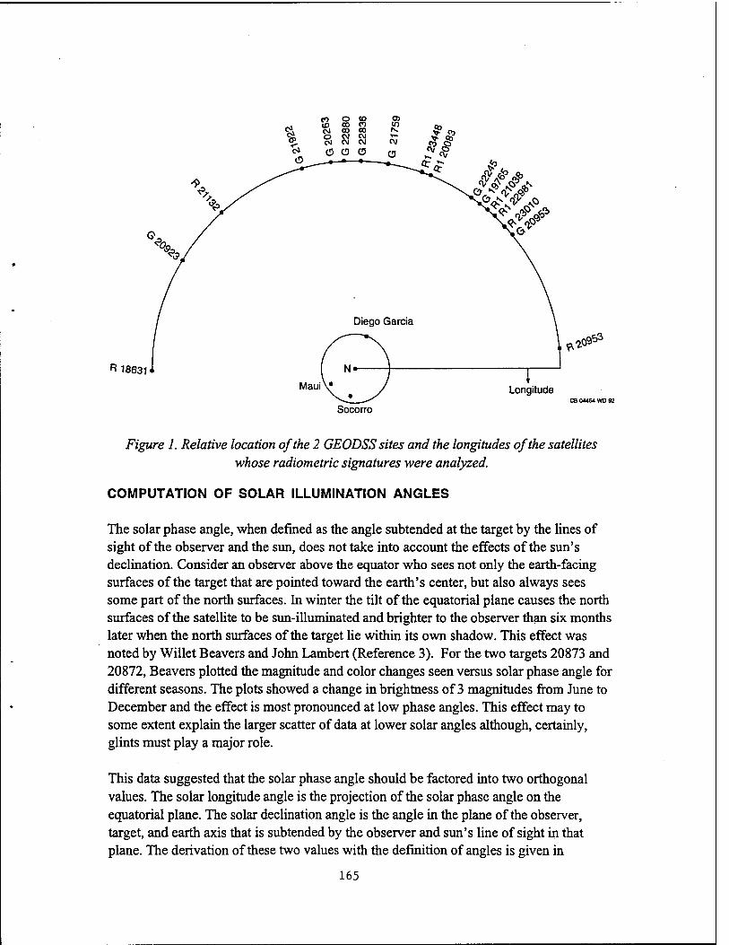
R 1863t

Longitude C8 04464 WD 92

Figure 1. Relative location of the 2 GEODSS sites and the longitudes of the satellites whose radiometric signatures were analyzed.

COMPUTATION OF SOLAR ILLUMINATION ANGLES

The solar phase angle, when defined as the angle subtended at the target by the lines of sight of the observer and the sun, does not take into account the effects of the sun's declination. Consider an observer above the equator who sees not only the earth-facing surfaces of the target that are pointed toward the earth's center, but also always sees some part of the north surfaces. In winter the tilt of the equatorial plane causes the north surfaces of the satellite to be sun-illuminated and brighter to the observer than six months later when the north surfaces of the target lie within its own shadow. This effect was noted by Willet Beavers and John Lambert (Reference 3). For the two targets 20873 and 20872, Beavers plotted the magnitude and color changes seen versus solar phase angle for different seasons. The plots showed a change in brightness of 3 magnitudes from June to December and the effect is most pronounced at low phase angles. This effect may to some extent explain the larger scatter of data at lower solar angles although, certainly, glints must play a major role.

This data suggested that the solar phase angle should be factored into two orthogonal values. The solar longitude angle is the projection of the solar phase angle on the equatorial plane. The solar declination angle is the angle in the plane of the observer, target, and earth axis that is subtended by the observer and sun's line of sight in that plane. The derivation of these two values with the definition of angles is given in

165

Appendix A. Also exampled are the parametric values used to calculate the values given in this study, using as an the catalog file number 3294 for the satellite 19765.

DATA ANALYSIS OF BRIGHTNESS VERSUS SOLAR ANGLES

Using a COTS 3D program, the normalized magnitude values were plotted versus the solar longitude angle and solar declination angle for five Raduga, three Raduga-1, and four Gorizont targets. For each target, a least-squares-fit to a parabola in two dimensions was performed using the relationship:

1. Mag= A+ B*SOL_LONG+C*SOL_LONGA2 + D*SOL_DEC + E*SOL_DECA2

This two-dimensional parabola was chosen since most objects exhibit a non-linear increase in brightness at low phase angles. Examples of these plots for each satellite class are shown in Figures 1-3. Each is a needle plot terminating in a solid black square, while the shadow plots showing magnitude as a function of only one parameter are cast as open squares on the appropriate wall. The magnitudes, normalized to a range of 1000 km, are plotted as a function of solar declination and solar longitude. The range in longitude represents relative locations during the viewing hours are the site. The range in solar declination covers the six-month viewing period when the declination is + 23 degrees. The continuous surface in figures labelled a) represents the best-fit figure as given by equation 1. The figure in labelled b) in each plot is the difference value between the fitted and actual value.

The goodness of fit was examined for each target in terms of the residual rms. The values for the four parameters are given in Table 3. The rms value is the residual rms after the fit. Attempts were made to reduce this value by eliminating values greater than 2 sigma, and in a few cases the rms values did decrease significantly. However, for the best-fit curves shown in Figures 2-4, no data points were excluded. Furthermore, even the signs of the parameters were not consistent with some targets showing an increase in brightness with solar angle and little correlation with the solar declination angle. This lack of correlation indicates that the brightness function is driven more by the complex scattering from the target than by the angle of solar illumination or it is an indication that the data has some inherent errors. Target number 18633 offers an opportunity to compare the GEODSS data with data taken with different sensors but at the same site as reported in Reference 5. Plotted in Figure 5 is the measured magnitude not normalized to a standard distance as a function of solar angle as observed using the MOTIF CMP sensor, the CCD sensor used by Beavers and the GEODSS data. The Beavers CCD data show a gradual increase in brightness as the solar angle decreases, but both the MOTIF and GEODSS data show considerable scatter of several magnitudes.

166

a) RADUGA18631

SolJLong Sol Dec

Magnitude

60 -30

b) RADUGA 18631

Sol_Long

>r 1-° -^^V^-... ...L 0.5 ■-••a..;

s_ f .Lo.o

L -0.5 ***•**«

--1.0

/ "**""*"/'* -1.5

-***^^**N**s^ / -2.0

10

30

Sol Dec

DIF

-30

Figure 2. a) The magnitude plotted as a function of the two solar angles for the RADUGA 18631 is shown as a needle plot with the magnitudes as black squares. The best-fit curve is shown as a net. The magnitude for each individual solar angle is projected on the walls

in open squares. In b) is shown the difference plot between the best-fit curve and the individual data points.

167

a) RADUGA-1 20083

SolJLong

3 Magnitude

60 -30

b) RADUGA-1 20083

Sol_Long Sol Dec

DIF

Figure 3. a) The magnitude plotted as a function of the two solar angles for the RADUGA 1 20083 is shown as a needle plot with the magnitudes as black squares. The best-fit curve is shown as a net. The magnitude for each individual solar angle is projected on the walls

in open squares. In b) is shown the difference plot between the best-fit curve and the individual data points.

168

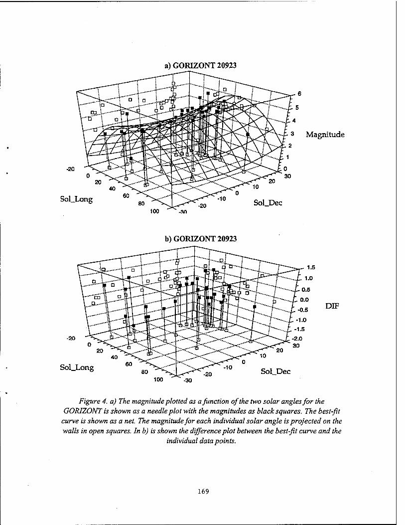
a) GORIZONT 20923

Sol_Long

3 Magnitude

b) GORIZONT 20923

Sol_Long Sol Dec

DIF

Figure 4. a) The magnitude plotted as a function of the two solar angles for the GORIZONT is shown as a needle plot with the magnitudes as black squares. The best-fit

curve is shown as a net. The magnitude for each individual solar angle is projected on the walls in open squares. In b) is shown the difference plot between the best-fit curve and the

individual data points.

169

18631 (RADUGA)

u

15

14

13

D 12

I W 11

8 10

D i •0-—I

i

6 rf13 Di

m-r

D"L

^ * ■ ! ■

! ü A AA j

rr

Bl i

D I D

SENSOR

■ GEODSS

▲ Beavers

D MOTIF

_1 I 1_QJ I I I I I 1 L- . , , I ,

10 20 30 40 50 60 70 80

PHASE ANGLE PEG)

Figure 5. Comparison of the GEODSS data with data reported by Lambert in Reference 5 for two sensors, a CCD camera, and the MOTIF CMP photometer.

Table 3. The two-dimensional linear and non-linear terms obtained from a best-fit of the data for each satellite to Equation 1. The units are magnitude for A, magnitude/degree for B andD and magnitude/degree2 for C andE. The rms reported is the residual after the fit

has been performed.

SATCAT NAME POINTS A B C D.E-3 E.E-3 RMS 18631 RADUGA 27 30501 -.001 .017 ..486 1.156 .524 21132 RADUGA 11 3.154 .021 -.022 .706 1,716 .124 22836 RADUGA 13 4.329 -.004 -.003 .048 -.310 .300 23010 RADUGA 13 3.378 -.009 .010 .557 .202 .380 23448 RADUGA 13 3.249 -.001 -.008 .311 1.032 .376 20083 RADUGA-1 23 4.274 .000 -.016 -.077 754 1.021 21038 RADUGA-1 19 3.568 -.015 -.005 .467 .531 .670 22981 RADUGA-1 12 3.069 .008 .014 .157 .903 1.045 20263 GORIZONT 21 3.378 -.009 .006 .229 .536 .812 20923 GORIZONT 29 2.408 .080 .007 -.896 .705 .568 20953 GORIZONT 19 2.308 -.027 .019 .635 2.904 1.360 21759 GORIZONT 11 4.233 .012 -.002 -.130 -.342 .692

Although the quality control for the GEODSS radiometric data has been formalized and appears to be routine, there are several sources of error that may be present in the GEODSS data. There are two opportunities within the bounds of written procedures and operational modes during photometric calibration that can affect the error and uncertainty in the visual brightness measurements. While the extinction ratio is measured before and

170

after each observation, the acceptance range is high, varying from 0.005 to 0.9. This wide range may serve as a check on the validity of the computation, but does not allow for the exclusion of data when the absorption is high or variable over a given night. As an example, the ETS site has reported that in the neighborhood of Socorro the skies are free of clouds only 46% of the time. Some of the archived data showed brightness changes that are consistent with clouds. The extinction ratio does not appear in the final archived data set, so it is not possible to assess the validity based on extinction ratio.

The second possibility for errors is that no filter is placed in the radiometer path during calibration or data acquisition. Calibration should be done against a "V" filter since the stars are not black bodies. This can result in an incorrect calibration if the operator, in his attempt to select a calibration star near the target, uses a star that does not match the effective color temperature of the sun. Additionally, preliminary evidence suggests that the satellites themselves exhibit color changes based on which materials on the satellite are illuminated at various times. This effect can also cause significant error.

There have been some attempts to measure the site-to-site agreement in radiometric calibration. This value is reported as +/- 0.1 magnitudes. If this is the case, the fluctuations are in fact caused by the complex scattering from the target surfaces. With extensive models available it is possible to model the scattering from these targets.

MODELING OF SATELLITE BRIGHTNESS

In other investigations only simple geometric shapes have been considered to estimate the radiometric signal and its dependence on the solar phase angle and aspect ratio observed at the receiver. This investigation plans to use available models with known surface reflectivities and BRDF's to predict the relative brightness as a function of the solar angles and the target aspect angle. In a small fraction of the records observed there is a continual slope to the magnitude data, indicating that the temporal resolution may need to be on the order of 10 minutes or less. TASAT will be used to simulate observations of a GORIZONT satellite. A detailed model generated by the Satellite Assessment Center will be used as the 'target' and renderings will be made to compute the equivalent stellar magnitude at different times in the particular observation file. It is also planned to make multiple renderings with small rotations to evaluate changes in magnitude caused by small motions, or wobble of the satellite.

SUMMARY AND CONCLUSIONS

The raw radiometric data electronically transmitted to LL/MIT from the GEODSS sites have been processed, corrected for transmission errors, reformatted and transported to Phillips Laboratory. The record of each radiometric observation has been extracted from

171

the tapes. A total of 250 magnitude values were present for four Gorizont, five Raduga and three Raduga 1 targets during the period from January to June 1995.

The solar phase angle has been factored into two components. The magnitude-versus- solar longitude angle and solar declination angle have been plotted and curves fit to each separate target. No clear trend is apparent in the data, with fitted parameters fluctuating with the three classes of targets. The residual rms, after fitting, remains around one visual magnitude. While possible errors to account for these fluctuations have been proposed, the major effort remains to use target models to predict the magnitude as a function of solar angles and target aspect ratio. This effort is currently in progress. Using current target models and most recent material property lists, the simulation program TASAT will be used to calculate the normalized brightness at the ECI coordinates and sites for each GEODSS observation.

ACKNOWLEDGEMENT

The authors wish to thank Tim Wallace and David Chan of Lincoln Laboratory/MIT for their initiative in gathering the GEODSS photometric records, correcting the transmission errors, and supplying the archived records in readable form.

REFERENCES

1. J.V. Lambert, R.E. Nachand, V.L.Porter and C, Stewart SDR: 15 June 1994 Multispectral Signatures of Near-Earth Satellites.

2. J.V. Lambert and G.E. Mavko,, Spectroscopic Signatures of Synchronous Satellites published in NORAD Spacecraft Identification Conference Proceedings (1975).

3. Willet Beavers and John Lambert at the SSW Meeting 23-24 June 1993.

4. John Lambert, Rockwell Space Operations. SDR: MOTIF FY95-01 30 November 1994. Interpretation of Geosynchronous Satellite Phase Angle Versus Magnitude Relationships.

5. John V. Lambert, Rockwell Space Operations and W.A. Kraszewski RPS, SDR; Phase Angle Versus Magnitude Relationships for Two Classes of Geosynchronous Satellites, April 1994, for AFSC.

172

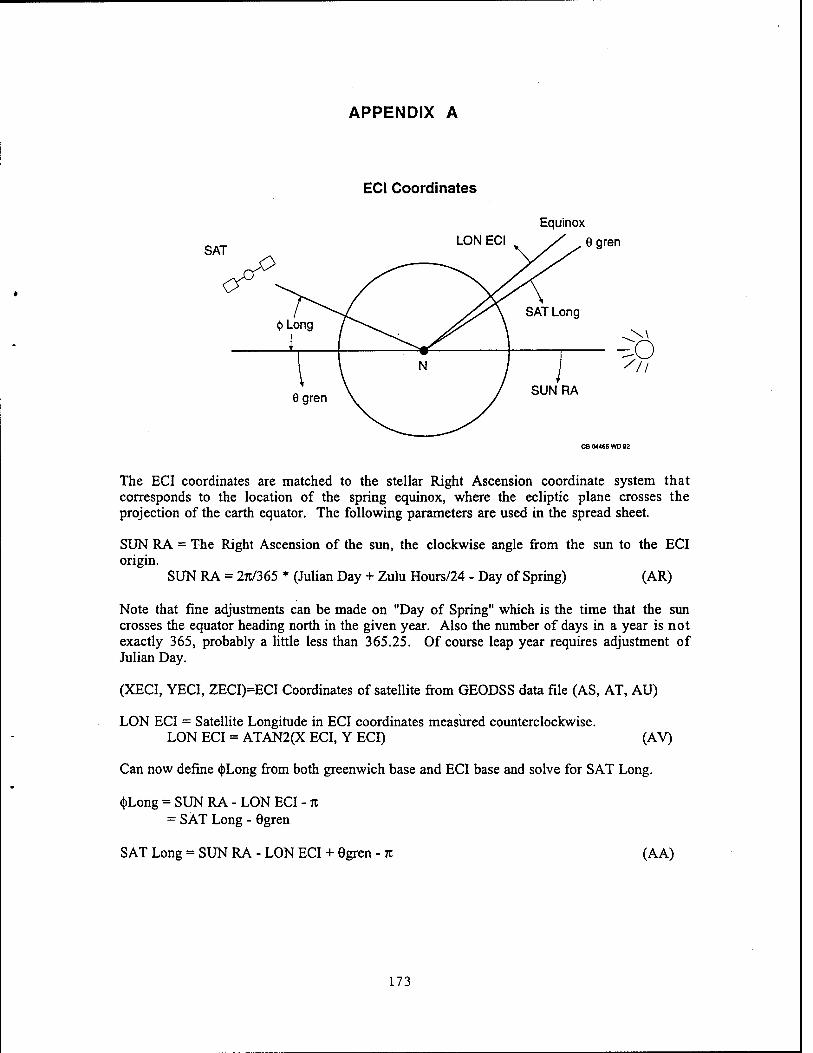
APPENDIX A

ECI Coordinates

SAT

Equinox LON ECI / e gren

CB 04465 WD 02

The ECI coordinates are matched to the stellar Right Ascension coordinate system that corresponds to the location of the spring equinox, where the ecliptic plane crosses the projection of the earth equator. The following parameters are used in the spread sheet.

SUN RA = The Right Ascension of the sun, the clockwise angle from the sun to the ECI origin.

SUN RA = 2n/365 * (Julian Day + Zulu Hours/24 - Day of Spring) (AR)

Note that fine adjustments can be made on "Day of Spring" which is the time that the sun crosses the equator heading north in the given year. Also the number of days in a year is not exactly 365, probably a little less than 365.25. Of course leap year requires adjustment of Julian Day.

(XECI, YECI, ZECI)=ECI Coordinates of satellite from GEODSS data file (AS, AT, AU)

LON ECI = Satellite Longitude in ECI coordinates measured counterclockwise. LON ECI = ATAN2(X ECI, Y ECI) (AV)

Can now define <|)Long from both greenwich base and ECI base and solve for SAT Long.

<|)Long = SUN RA - LON ECI - re = SAT Long - Ggren

SAT Long = SUN RA - LON ECI + Ggren - n (AA)

173

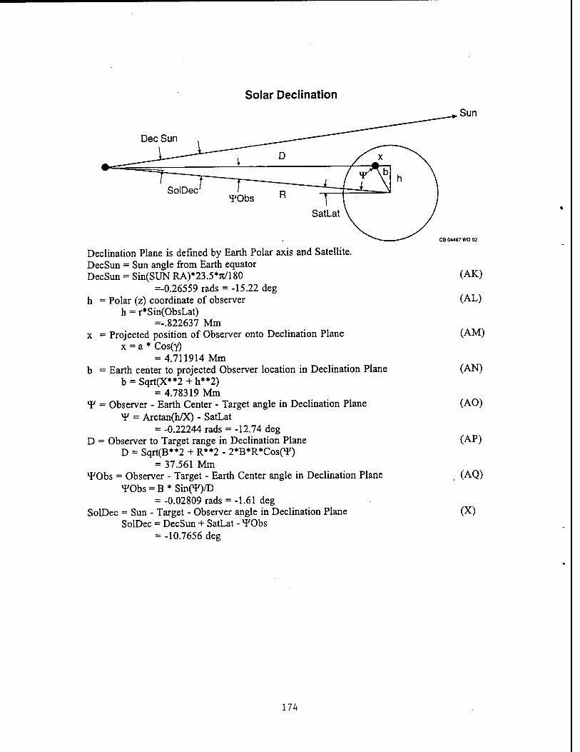
Solar Declination

Dec Sun

Sun

SolDec

CB 04467 WD 92

Declination Plane is defined by Earth Polar axis and Satellite. DecSun = Sun angle from Earth equator DecSun = Sin(SUN RA)*23.5*n/180

=-0.26559 rads = -15.22 deg h = Polar (z) coordinate of observer

h = r*Sin(ObsLat) =-.822637 Mm

x = Projected position of Observer onto Declination Plane x = a * Cos(Y)

= 4.711914 Mm b = Earth center to projected Observer location in Declination Plane

b = Sqrt(X**2 + h**2) = 4.78319 Mm

*F = Observer - Earth Center - Target angle in Declination Plane V = Arctan(h/X) - SatLat

= -0.22244 rads = -12.74 deg D = Observer to Target range in Declination Plane

D = Sqrt(B**2 + R**2 - 2*B*R*Cos(4/) = 37.561 Mm

TObs = Observer - Target - Earth Center angle in Declination Plane TObs = B * SinOF)/D

= -0.02809 rads = -1.61 deg SolDec = Sun - Target - Observer angle in Declination Plane

SolDec = DecSun + SatLat - ^Obs = -10.7656 deg

(AK)

(AL)

(AM)

(AN)

(AO)

(AP)

(AQ)

(X)

174

Solar Longitude

Sol Long

* r==::::::;^~-j--zobs ""I1 0DS ^"^-v/?"^---^ R^COS (SatLat) ^\^^"-~^-^^Observer

/*\ / \ a J

Ggren

<t> Long /^'^OL'

1 r N

C8 044MWD«

For catalog file # 3294 Satellite 19765 r = Earth radius = 6.38 Mm R ECI = ECI range to satellite from GEODSS data (Z)

R ECI = SQRT(X ECIA2 + Y ECIA2 + Z ECIA2) SatLong = Satellite Longitude (+West, -East) = 4.288 rads = 245.7 DEG (AA) SatLat = Satellite Latitude = ASIN(Z ECI/R ECI) (AB) ObsLong = Observer Longitude = 287.55 deg = 5.0187 rads (AC) ObsLat = Observer Latitude = -7.41 deg = -.1293 rads (AD) Ggren = Greenwich location from Zulu Time (AE)

Ggren =(n /12)*(Hr + Min/60 + Sec/3600) =(« /12)*(14. + 37./60 + 20.29/3600) = 3.82811

<|>long = Sun - Target - Earth angle (AF) ((»long = SatLong - Ogren

= 0.45997 rads = 26.35 deg Y = Target - Earth - Observer angle (AG)

Y = SatLong - ObsLong = -0.7306 rads = -41.86 deg

a = Radius to observer from Earth polar axis (AH) a = r * cos(ObsLat)

= 6.326742 Mm Zobs = Projected distance from observer to target (AI) Zobs = a**2 + R*Cos(SatLat)**2 - 2*a*R*Cos(SatLat)*Cos(g)

= 37.685 Mm <|)obs = Earth - Target - Observer angle (AJ)

<(>obs = arcsin(a*sin(Y)/Zobs = -0.11227 rads = -6.432 deg

SolLong = Sun - Target - Observer angle in Longitude plane (W) SolLong = <|)long + <])obs

= 19.9218 deg

175

Space Object Identification Using Optical Aperture Synthesis

S.R. Restaino (USAF/Phillips Lab.) ,RJ. McBroom (Rockwell Power Systems), J.T. Baker (Rockwell Power Systems), D.A. Nahrstedt (Rockwell Power Systems), D.M.

Payne (W.J. Schäfer), R.A. Carreras (USAF/Phillips Lab.), D.W. Tyler (W.J. Schäfer), K.J. Schulze (W.J. Schafer), G.C. Loos (USAF/Phillips Lab.)

Abstract

The results of two full-scale field experiments are reported which demonstrate the utility of aperture synthesis for visible wavelength, high-resolution interferometric imaging of space objects. The first experiment demonstrate non-redundant pupil masking to minimize image distortion due to atmospheric turbulence. Observations are made using a multi- aperture mask with the 80-cm Beam Director/Tracker telescope at the Maui Space Surveillance Site (MSSS). Reconstructed, near diffraction-limited images of man made satellite are compared with simultaneous observations from the Compensated Imaging System (CIS) on the MSSS 1.6 meter telescope. The second experiment demonstrates the use of single mode (SM) optical fibers for spatial filtering, and beam relay and recombination, to synthesize 4-meter class resolution by coupling two 1.2 meter telescopes. White-light fringes are obtained from Arcturus (a Bootis) demonstrating the potential for generating the angular spectrum of the object.

Introduction

There are two main limitation for high-angular resolution imaging of exoatmospheric objects from the ground. The first limit is imposed by manufacturing processes and affects the attainable size of an optical system, this is related to the maximum high spatial frequency observable. The limit right now, and for the foreseeable future, is around 10 meters. The other limiting factor is the turbulence of the Earth's atmosphere that limits the effective diameter of the optical receiver. Several techniques have been proposed to deal with these limiting factors. Here we present the results of two experiments dealing with the use of synthetic aperture. The first experiment described here is a pupil masking experiment. The basic idea is that through the use of a mechanical mean, the mask, only certain spatial frequencies are admitted through the system, in this way we can control the distortion of the high spatial frequency region due to the atmospheric turbulence. Furthermore we were able to demonstrate for the first time, imaging of complex object through a diluted pupil.

The second experiment deals with the use of SM fibers for beam relay and recombination. We linked the two 1.2 m telescopes of the Maui Tracking and Identification Facility (MOTIF) together achieving a 4 meter class resolution in one direction. The use of SM

177

fibers as beam transporters in long baseline optical interferometry has been suggested by few authors1'2

The most useful characteristics that SM fibers offer to beam transport and recombination are summarized below:

Spatial filtering: i.e. the fibers filter most of the high frequency noise introduced into the wavefront by the turbulent atmosphere.

• High level of coherence preservation: The coherence of the spatially filtered wavefront is preserved as the light propagates through the fiber.

• Almost lossless transport of energy: modern SM fibers can be manufactured with an extremely low power loss'capability. This is thanks to the communication industry needing to transport signals for many miles with the smallest loss possible.

The main drawback of using fibers is their coupling efficiency, i.e. the amount of light than can be injected into the fibers. The main cause of this loss is due to the physical dimensions of the core, the region of the fiber that carries the signal, that usually is a few microns in diameter. For this reason there have being few experimental testing on telescopes, especially at visible wavelengths where the atmospheric turbulence is more severe than at longer wavelengths. A preliminary experiment, without control loops, has been carried out in the near infra-red region recently by Ref. 3.

Experimental results

A. The pupil mask experiment.

The basic layout of the experiment is outlined in Fig. 1. Several masks with different hole diameter and arrangement were used. In Fig. 2 is illustrated the experimental results of comparing the full aperture of the telescope with two different masks. The plot shows the circularly integrated averaged power spectrum of the star a Bootis. 50 frames of 50 millisec of exposure time each were used for the time average, and divided by the variance. The three plots referee to the full pupil, a pupil mask with 5 holes and 20 cm for the hole diameter, and finally a mask with 11 holes with a diameter of 10 cm. It is evident the gain in the high spatial frequency region with the 11 holes mask. The measured r0, coherence diameter of the atmosphere, the night of the observations is 10 cm at the dome of the 1.6 m telescope, few meters away from our telescope. This also stresses the importance of matching the diameter hole with the coherence diameter of the atmosphere. This matching will enable the removal of the redundancy noise introduced by the atmospheric turbulence in a fully redundant pupil. A description of the effect of spatial filtering through a pupil mask can be found in Ref. 2,3. Here we will limit ourselves to an heuristic explanation based on the basic interferometric process of the image formation. A pair of points in the entrance pupil of an imaging system will interfere and give a set of fringes in the image plane. Since there are many points with the same

178

distance we will have many sets of fringes with the same frequency. The effect of the atmospheric turbulence is to shift randomly these fringes, and when they are summed in the image plane, because of their relative random shifts, a depressed fringe will result (this is what we called redundant noise). This is also a way to physically explain the image blur due to the atmospheric turbulence. If we now put a non redundant mask, i.e. each pair's separation is present only once, and as long as the diameter of the holes is equal or less than the coherence diameter of the atmosphere, each pair of holes will produce a unique fringe with an unique frequency. When the atmosphere moves randomly the fringes, the effect will not be to decrease the overall visibility because the fringes will have different frequencies. An analysis of the Signal-to-Noise-Ratio (SNR) characteristics of such a non redundant mask can be found in Ref. 2,3. In Fig. 3 is shown an image of the space station MIR acquired through a pupil mask. The image is a mosaic of several images due to the fact that the object was much larger than our field of view. In Fig. 3 is also noted the diffraction limit of the telescope. It is clear that the imagery is almost diffraction limited. This demonstrate the capabilities of a nonredundant pupil mask. In condition of high SNR (i.e. SNR > 1) a non-redundant mask can be an economical substitute of adaptive optics for achieving high resolution images of exoatmospheric objects.

B The Single Mode Fiber Experiment.

The Maui Space Surveillance Site (MSSS) was chosen as the site of this experiment due to the existence of a unique facility, the MOTIF telescope. The MOTIF consist of two 1.2 m telescopes co-mounted in a binocular type of arrangement. The center to center distance of the two telescopes is 4 m. The main part of the Phillips Lab experiment was composed of two independent tilt-loop controllers4 with the coupling optics, for each telescope. The other main controller was the strain-controller loop. A schematic diagram of the optical lay-out is shown in Fig. 4. The tilt controller is described in detail in Ref. 4 it consists of a commercial quad-cell as the sensor and four voice-coil actuators as the tilt mirrors actuators. The maximum bandwidth achievable at closed loop is of 500 Hz. The two telescopes have a different optical configuration and the re-imaging optics for both telescopes was different in order to achieve the same numerical aperture on the fibers. The detector used to record the fringes was a commercial CCD camera with a Kodak chip having 768X512 pixels, of which we used an area of 128X64 pixels. As an astronomical source we used the bright star a Bootis (Arctururs) visual magnitude - 0.2. We were able to collect several frames of data with one telescope with the tilt corrector on or off in order to measure the coupling efficiency in both cases. When the tilt corrector was turned off we measured an average (using 50

179

frames of data) of 0.9% coupling efficiency. With the tilt corrector on we achieved an average of 3% in coupling efficiency. This well matches the theoretical prediction given by the following expression:

D 1 + 1.06/y^j +WM\D

where r\ is the maximum coupling efficiency, r0 is the coherence diameter of the atmosphere, D is the diameter of the telescope and u is a parameter that is equal to 1 if the tilt is removed and equal to 0 for tilt not removed. D is 120 cm and r0 was approximately 12 cm. In fig. 5 are shown, side by side, a frame of fringes obtained with the laser illuminating both telescopes and a frame of fringes obtained from the star. The average measured visibility of the fringes is of 33%. It is to be noted that the spacing of the fringes changes due to a motion of the

recombination beam splitter during the day (the laser fringes were acquired in the morning during alignment procedures and the stellar fringes were acquired several hours later during normal observing operations). Furthermore, the stellar fringes are visible over a smaller area due to the spectral bandwidth used (100 nm).

Conclusions

We have reported the first observation of complex objects, satellites, with a non-redundant mask, showing that it is possible to obtain near diffraction limited images with such a technique. Furthermore we have reported the first controlled link between two independent telescopes at visible wavelengths using SM fibers. The use of single mode fibers can improve dramatically the cost of ground-based optical interferometers, for deep space surveillance, and has the potential for larger savings with spaced-based ones.

References 1. Froehly C. (1981) Proc ESO Conference on Scientific Importance of High Angular Resolution at IR and optical wavelength. 2. Shacklan S. and Roddier F., Appl. Opt. 27, 2334 (1988) 3. Coude du Furesto V., Maze G., Ridgway S., Astro. Soc. of Pac. Conf. Ser. 37 (1992) 4. Baker I, Dymale R., Carreras R., Restaino S.R., Journal of Elect. Eng. and Controls (submitted)

5. Fried D., J. Opt. Soc. Am. 56 1372 (1966).

180

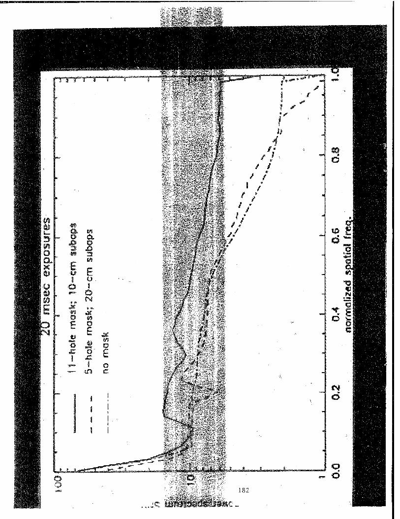
B u »UB^H 3

W ;?§9HHH Q 1st«SHH^H Q*

X HS &l

M •0 0»

'$$&B mm ^

11 » E

o

M

m

o

o

s o

MIR - 5 Hole Mask - Deconvolved Mosaic

183

"^

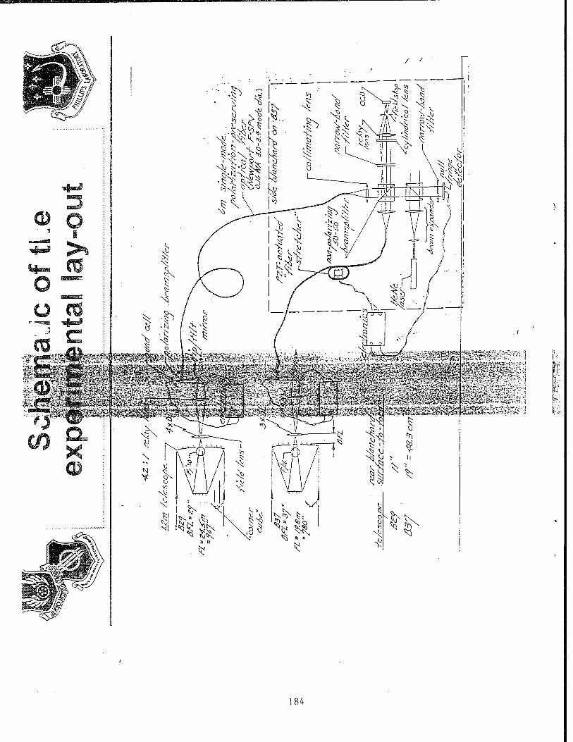
184

■i#£

REPORT DOCUMENTATION PAGE Form Approved OMB No. 0704-0188

Public reporting burden for this collection of information is estimated to average 1 hour per response, including the time for reviewing instructions, searching existing data sources, gathering and maintaining the data needed, and completing and reviewing the collection of information. Send comments regarding this burden estimate or any other aspect of this collection of information, Including suggestions for reducing this burden, to Washington Headquarters Services, Directorate for Information Operations and Reports, 1215 Jefferson Davis Highway, Suite 1204, Arlington, VA 22202-4302, and to the Office of Management and Budget, Paperwork Reduction Project (07M-01B8I. Washington. DC 20503.

1. AGENCY USE ONLY {Leave blank) 2. REPORT DATE

4 April 1996

3. REPORT TYPE AND DATES COVERED

Project Report

4. TITLE AND SUBTITLE

Proceedings of the 1996 Space Surveillance Workshop

5. FUNDING NUMBERS

C — F19628-95-C-0002 6. AUTHOR(S)

K.P. Schwan (Editor)

7. PERFORMING ORGANIZATION NAME(S) AND ADDRESS(ES)

Lincoln Laboratory, MIT

244 Wood Street

Lexington, MA 02173-9108

8. PERFORMING ORGANIZATION REPORT NUMBER

STK-245 Volume I

9. SPONSORING/MONITORING AGENCY NAME(S) AND ADDRESS(ES)

ESC

Hanscom Air Force Base

Bedford, MA 01730

10. SPONSORING/MONITORING AGENCY REPORT NUMBER

ESC-TR-96-026

11. SUPPLEMENTARY NOTES

None

12a. DISTRIBUTION/AVAILABILITY STATEMENT


12b. DISTRIBUTION CODE

13. ABSTRACT {Maximum 200 words)

The fourteenth Annual Space Surveillance Workshop hosted by MIT Lincoln Laboratory was

held 2—4 April 1996. The purpose of this series of workshops is to provide a forum for the presentation

and discussion of space surveillance issues. This Proceedings documents most of the presentations,

with minor changes where necessary.

14. SUBJECT TERMS 15. NUMBER OF PAGES

194

16. PRICE CODE

17. SECURITY CLASSIFICATION

OF REPORT

Unclassified

18. SECURITY CLASSIFICATION OF THIS PAGE

Unclassified

19. SECURITY CLASSIFICATION OF ABSTRACT

Unclassified

20. LIMITATION OF ABSTRACT

Same as report

NSN 7540-01-280-5500 Standard Form 298 (Rev. 2-89) Prescribed by AMSI Std. 239-18 298-102

project report stk-245 volume i - defense technical … · project report stk-245 volume i ......

Documents