proof-theoretic methods in nonclassical logic … methods in nonclassical logic — an introduction...

Proof-Theoretic Methods in Nonclassical Logic

— an Introduction

Hiroakira Ono

JAIST, Tatsunokuchi, Ishikawa, 923-1292, Japan

[email protected]

1 Introduction

This is an introduction to proof theory of nonclassical logic, which is directed atpeople who have just started the study of nonclassical logics, using proof-theoreticmethods. In our paper, we will discuss only its proof theory based on sequentcalculi. So, we will discuss mainly cut elimination and its consequences. As thisis not an introduction to sequent systems themselves, we will assume a certainfamiliarity with standard sequent systems LK for the classical logic and LJ for theintuitionistic logic. When necessary, readers may consult e.g. Chapter 1 of ProofTheory [43] by Takeuti, Chapters 3 and 4 of Basic Proof Theory [45] by Troel-stra and Schwichtenberg, and Chapter 1 of the present Memoir by M. Takahashi[41] to supplement our paper. Also, our intention is not to give an introductionof nonclassical logic, but to show how the standard proof-theoretic methods willwork well in the study of nonclassical logic, and why certain modifications will benecessary in some cases. We will take only some modal logics and substructurallogics as examples, and will give remarks on further applications. Notes at the endof each section include some indications for further reading.

An alternative approach to proof theory of nonclassical logic is given by usingnatural deduction systems. As it is well-known, natural deduction systems areclosely related to sequent calculi. For instance, the normal form theorem in naturaldeduction systems corresponds to the cut elimination theorem in sequent calculi.So, it will be interesting to look for results and techniques on natural deductionsystems which are counterparts of those on sequent calculi, given in the presentpaper.

The present paper is based on the talk given at MSJ Regional Workshop onTheories of Types and Proofs at Tokyo Institute of Technology in September, 1997,and also on the introductory talk on proof theory in Logic Summer School 1998, atAustralian National University in January, 1998. The author would like to express

207

208 h. ono

his thanks to M. Takahashi for offering him a chance of writing an introductorypaper in this field, and to Bayu Surarso, M. Bunder, R. Gore, A. Maruyama, T.Shimura and M. Takano for their helpful comments.

1.1 What is proof theory?

The main concern of proof theory is to study and analyze structures of proofs.A typical question in it is “what kind of proofs will a given formula A have, if itis provable?”, or “is there any standard proof of A?”. In proof theory, we want toderive some logical properties from the analysis of structures of proofs, by antici-pating that these properties must be reflected in the structures of proofs. In mostcases, the analysis will be based on combinatorial and constructive arguments. Inthis way, we can get sometimes much more information on the logical propertiesthan with semantical methods, which will use set-theoretic notions like models,interpretations and validity.

On the other hand, the amount of information which we will get from thesesyntactic analyses depends highly on the way of formalizing a given logic. Thatis, in some formulations structures of proofs will reflect logical properties moresensitively than in others. For instance, Hilbert-style formal systems were popularin the first half of this century, which consist usually of many axiom schemes with afew rule of inference, including modus ponens. This formulation is in a sense quiteflexible and is convenient for representing various logics in a uniform way. On theother hand, the arbitrariness of the choice of axioms of a given logic in Hilbert-styleformulation tells us the lack of sensitivity to logical properties, although to someextent the proof theory based on Hilbert-style formal systems had been developed.

Then, G. Gentzen introduced both natural deduction systems and sequent cal-culi for the classical logic and the intuitionistic one in the middle of 1930s. Themain advantage of these two kinds of systems comes from the fact that there is astandard proof of a given formula as long as it is provable. This fact is certified bynormal form theorem in natural deduction systems and by cut elimination theoremin sequent calculi. Moreover, it turned out that “standard” proofs reflect someof logical properties quite well. For instance, one can derive the decidability, andmoreover the decision procedure, for a propositional logic by using the existenceof “standard” proofs. In this way, we can get much more information on logicalproperties from proofs in these formulations. This fact has led to the success ofproof theory based on natural deduction systems and sequent calculi, in particularto consistency proofs of Peano arithmetic and its extensions.

1.2 Proof-theoretic methods in nonclassical logic

Our goal of the present paper is to show the usefulness ( and the limitations )of proof-theoretic methods by taking appropriate examples from sequent calculifor nonclassical logic, in particular for modal and substructural logics. As will beexplained later, proof-theoretic methods will give us deeper results than semanticalones do, in particular in their computational aspects. For instance, the cut elimi-nation theorem for a propositional logic implies often its decidability, and the proof

proof-theoretic methods in nonclassical logic 209

will give us an effective decision procedure ( see Sections 4 and 5 ). Also, Mae-hara’s method of proving Craig’s interpolation theorem will give us an interpolanteffectively ( see Section 6 ).

The study of computational aspects of logics is particularly important in theirapplications. Modal logics cover epistemic logics, deontic logics, dynamic logics,temporal logics and so on, which will give theoretical foundations of artificial in-telligence and software verification. Also, substructural logics include linear logicand Lambek calculus, which will give us a theoretical basis of concurrent processes( see [31] ) and categorial grammar, respectively. This is the reason why we willfocus on modal and substructural logics in the present paper.

We note here that most of automatic theorem provers at present are designedand implemented on the basis of Hilbert-style formal systems because of the mod-ularity of these systems, while many of interactive theorem provers are based onGentzen-style systems.

But, when we gain, we may also lose. As mentioned above, proof-theoreticmethods work well mostly in the case where the existence of “standard” proofs isguaranteed. But as a matter of fact, this happens to hold only for a limited numberof nonclassical logics. On the other hand, one may have much more interest inthe study of a class of nonclassical logics, than in that of particular logics. Insuch a case, proof-theoretic methods will be useless. Semantical and algebraicmethods will work well instead, although results obtained by them will usuallylack constructive and computational features. For example, Maksimova proved in[27] that the interpolation theorem holds only for seven intermediate propositionallogics, i.e. logics between the intuitionistic logic and the classical. We can useproof-theoretic methods to show that the interpolation theorem holds for each ofthese seven logics. But, when we show that the interpolation theorem doesn’t holdfor any other logics, there will be no chance of using these proof-theoretic methods.In this sense, we can say that proof-theoretic methods and semantical ones arecomplementary to each other. In fact, sometimes it happens that a general resultshown by a semantical method was originally inspired by a result on particularlogics proved by a proof-theoretic method.

The present paper consists of eight sections. In Section 2, we will introducesequent calculi for logics discussed in this paper. Among others, sequent calculifor standard substructural logics will be given. As this is an introductory paper,extensions of sequent calculi like labelled deduction systems, display logics andsystems for hypersequents will not be treated here. Cut elimination theorem willbe discussed in Section 3. After a brief outline of the proof for LJ, we will indicatehow we should modify the proof when we show the cut elimination theorem forsubstructural logics. An important consequence, and probably the most importantconsequence, of cut elimination theorem is the subformula property. In the endof Section 3, we will introduce Takano’s idea of proving the subformula propertyof sequent calculi for some modal logics, for which the cut elimination theoremdoesn’t hold.

210 h. ono

In Sections 4 and 5, the decision problem will be discussed. It will be shown thatthe contraction rule will play an essential role in decidability. In many cases, Craig’sinterpolation theorem can be derived from the cut elimination theorem by usingMaehara’s method. This is outlined in Section 6. Another application of the cutelimination theorem in the author’s recent joint paper [30] with Naruse and BayuSurarso gives a syntactic proof of Maksimova’s principle of variable separation.The topic is outlined in Section 7. A short, concluding remark is given in the lastsection.

1.3 Notes

We will give here some basic literature on proof theory. Hilbert-Ackermann [20]developed the first, comprehensive study of proof theory based on a Hilbert-styleformulation. In his paper [17] in 1935 Gentzen introduced both natural deductionsystems and sequent calculi for the classical logic and the intuitionistic. The paperbecame the main source of studies on proof theory developed later. As for furtherinformation on natural deduction, see e.g. [37, 40, 45, 10]. Another way of for-malizing logics, which is closely related to one using sequent calculi, is the tableaumethod. For the details, see e.g. [16]. As for recent developments of proof theoryin general, consult [6].

2 Sequent Calculi for Nonclassical Logic

We will introduce several basic systems of sequent calculi discussed in our paper.First, we will introduce sequent calculi LK and LJ for the classical predicate logicand the intuitionistic one, respectively. Then, we will introduce some of sequentcalculi for modal logics, by adding rules or initial sequents for the modal operator2, and also sequent calculi for substructural logics, by deleting some of structuralrules either from LK or from LJ.

2.1 Sequent calculi LK and LJ

We assume here that the language L of LK and LJ consists of logical con-nectives ∧,∨,⊃ and ¬ and quantifiers ∀ and ∃. The first-order formulas of Lare defined in the usual way. A sequent of LK is an expression of the formA1, . . . , Am → B1, . . . , Bn, with m,n ≥ 0. As usual, Greek capital letters Σ, Λ, Γetc. denote ( finite, possibly empty ) sequence of formulas. Suppose that a sequentΣ → Π is given. Then, any formula in Σ ( Π ) is called an antecedent ( a succedent )of the sequent Σ → Π.

In the following, we will introduce first a formulation of the sequent calculusLK, which is slightly different but not in an essential way from the usual one.Initial sequents of LK are sequents of the form A → A. Rules of inference of LKconsist of the following;

Structural rules:


Weakening rule:

Γ, Σ → ∆

Γ, A, Σ → ∆(w →)

Γ → Λ, Θ

Γ → Λ, A, Θ(→ w)

Contraction rule:

Γ, A,A, Σ → ∆

Γ, A, Σ → ∆(c →)

Γ → Λ, A,A, Θ

Γ → Λ, A, Θ(→ c)

Exchange rule:

Γ, A,B, Σ → ∆

Γ, B,A, Σ → ∆(e →)

Γ → Λ, A,B, Θ

Γ → Λ, B,A, Θ(→ e)

.

Cut rule:

Γ → A, Θ Σ, A, Π → ∆

Σ, Γ, Π → ∆, Θ

Rules for logical connectives:

Γ → A, Θ Π, B, Σ → ∆

Π, A ⊃ B, Γ, Σ → ∆, Θ(⊃→)

Γ, A → B, Θ

Γ → A ⊃ B, Θ(→⊃)

Γ, A, Σ → ∆

Γ, A ∧ B, Σ → ∆(∧1 →)

Γ, B, Σ → ∆

Γ, A ∧ B, Σ → ∆(∧2 →)

Γ → Λ, A, Θ Γ → Λ, B, Θ

Γ → Λ, A ∧ B, Θ(→ ∧)

Γ, A, Σ → ∆ Γ, B, Σ → ∆

Γ, A ∨ B, Σ → ∆(∨ →)

Γ → Λ, A, Θ

Γ → Λ, A ∨ B, Θ(→ ∨1)

Γ → Λ, B, Θ

Γ → Λ, A ∨ B, Θ(→ ∨2)

Γ → A, Θ

¬A, Γ → Θ(¬ →)

Γ, A → Θ

Γ → ¬A, Θ(→ ¬)

Rules for quantifiers:

Γ, A[t/x], Σ → ∆

Γ,∀xA, Σ → ∆(∀ →)

Γ → Λ, A[z/x], Θ

Γ → Λ,∀xA, Θ(→ ∀)

Γ, A[z/x], Σ → ∆

Γ,∃xA, Σ → ∆(∃ →)

Γ → Λ, A[t/x], Θ

Γ → Λ,∃xA, Θ(→ ∃)

.

212 h. ono

Here, A[z/x] ( A[t/x] ) is the formula obtained from A by replacing all free occur-rence of x in A by an individual variable z ( a term t, respectively ), but avoidingthe clash of variables. Also, in rules for quantifiers, t is an arbitrary term and z isan arbitrary individual variable not occurring in the lower sequent. ( Usually, thecut rule is considered to be one of the structural rules. For convenience sake, wewill not include it among the structural rules in our paper. )

Sequents of the sequent calculus LJ for the intuitionistic logic are expressionsof the form A1, . . . , Am → B where m ≥ 0 and B may be empty. Initial sequentsand rules of inference of LJ are obtained from those of LK in the above, first bydeleting both (→ c) and (→ e) and then by assuming moreover that both Λ and Θare empty and that ∆ consists of at most one formula. Proofs and the provabilityof a given sequent in LK or LJ are defined in a usual way. As usual, we say thata formula A is provable in LK ( LJ ), if the sequent → A is provable in it. Forformulas A and B, we say that A is logically equivalent to B in LK ( LJ ) whenboth A ⊃ B and B ⊃ A are provable in LK ( LJ, respectively ).

In the following, sometimes we will concentrate only on propositional logics. Insuch a case, LK and LJ mean the sequent calculi in the above, which deal onlywith sequents consisting of propositional formulas and which have only rules forlogical connectives. To emphasize this, we call them, propositional LK and LJ.

2.2 Adding modal operators

We will discuss two types of nonclassical logic in this paper. Logics of thefirst type can be obtained from classical logic by adding new logical operatorsor connectives. Particularly interesting nonclassical logics of this type are modallogics. Modal logics usually have unary logical operators 2 and 3, called modaloperators. There are many variations of modal logics. Some will contain manymodal operators and some will be based on logics other than classical logic.

We will discuss here sequent calculi for some standard modal propositional logicsas a typical example. In both of them, we assume that 3A is an abbreviation of¬2¬A. Thus, we suppose that our language L2 for modal logics consists of ( thepropositional part of ) L with a unary operator 2, which is usually read as “it isnecessary” and called the necessity operator. Now, consider the following axiomschemes:

K: 2(A ⊃ B) ⊃ (2A ⊃ 2B),T: 2A ⊃ A,4: 2A ⊃ 22A,5: 3A ⊃ 23A.

A Hilbert-style system for the modal logic K is obtained from any Hilbert-stylesystem for the classical propositional logic ( with modus ponens as its single rule ofinference ) by adding the axiom scheme K and the following rule of necessitation;

from A infer 2A.


Hilbert-style systems for modal logics KT, KT4 and KT5 are obtained from Kby adding T, T and 4, and T and 5, respectively. Traditionally, KT4 and KT5are called S4 and S5, respectively.

Now, we will introduce sequent calculi for these modal logics. A sequent calculusGK for K is obtained from LK by adding the following rule;

Γ → A2Γ → 2A

(2).

Here, 2Γ denotes the sequence of formulas 2A1, . . . ,2Am when Γ is A1, . . . , Am.Moreover, 2Γ is the empty sequence when Γ is empty. Consider moreover thefollowing three rules;

A, Γ → ∆

2A, Γ → ∆(2 →)

2Γ → A2Γ → 2A

(→ 21).

2Γ → 2∆, A

2Γ → 2∆,2A(→ 22)

.

Note here that the rule (2) can be derived when we have both (2 →) and(→ 21) and that (→ 21) is obtained from (→ 22) by assuming that ∆ is empty.The sequent calclus GKT is obtained from GK by adding the rule (2 →). Thesequent calculi GS4 and GS5 are obtained from LK by adding the rules (2 →)and (→ 21), and the rules (2 →) and (→ 22), respectively. We can show thefollowing.

Theorem 1 For any formula A, A is provable in K if and only if → A is provablein GK. This holds also between KT and GKT, between S4 and GS4, and betweenS5 and GS5.

2.3 Deleting structural rules

Nonclassical logics of the second type can be obtained either from classicallogic or from intuitionistic logic, by deleting or restricting structural rules. Theyare called substructural logics. Lambek calculus for categorial grammar, linear logicintroduced by Girard in 1987, relevant logics, BCK logics ( i.e. logics withoutcontraction rules ) and Lukasiewicz’s many-valued logics are examples of substruc-tural logics. Lambek calculus has no structural rules and linear logic has onlyexchange rules. Relevant logics have usually the contraction rules, but lack weak-ening rules. Lukasiewicz’s many-valued logics form a subclass of logics withoutcontraction rules.

Our basic calculus FL ( called the full Lambek calculus ) is, roughly speaking,the system obtained from the the sequent calculus LJ by deleting all structuralrules. We will also extend our language for the following reasons.

214 h. ono

In the formulation of the classical and the intuitionistic logic, we will sometimesintroduce propositional constants like ⊤ and ⊥ to express the constantly true propo-sition and false proposition, respectively. When we have these constants, we willtake the following sequents as the additional initial sequents:

1. Γ → ⊤2. Γ,⊥, Σ → ∆

where Γ, Σ and ∆ may be empty. ( We can dispense with ⊤, as it is logicallyequivalent to ⊥ ⊃ ⊥. ) It is easy to see that for any formula A which is provablein LK or LJ, A is logically equivalent to ⊤ in it. Note here that we need theweakening rule to show that ⊤ ⊃ A is provable, though A ⊃ ⊤ follows alwaysfrom the above 1. We can also show by the help of the weakening rule that ¬A islogically equivalent to A ⊃ ⊥ in either of LK and LJ.

These facts suggest to us that we may need special considerations for logicswithout the weakening rule. To make the situation clearer, let us introduce twomore propositional constants t and f, and assume the following initial sequents andrules of inference for them:

3. → t

4. f →

Γ, Σ → ∆

Γ, t, Σ → ∆(tw)

Γ → Λ, Θ

Γ → Λ, f, Θ(fw)

These initial sequents and rules mean that t ( f ) is the weakest ( strongest )proposition among provable formulas ( contradictory formulas, respectively ) andthat ¬A is logically equivalent to A ⊃ f. It can be easily seen that t and ⊤ ( andalso f and ⊥ ) are logically equivalent to each other, when we have the weakeningrule.

In LK, we can show that a sequent A1, . . . , Am → B1, . . . , Bn is provable ifand only if the sequent A1 ∧ . . . ∧ Am → B1 ∨ . . . ∨ Bn is provable. Thus, wecan say that commas in the antecedent of a given sequent mean conjunctions, andcommas in the succedent mean disjunctions. But, to show the equivalence of theabove two sequents, we need both weakening and the contraction rules. Thus, insubstructural logics we cannot always suppose that commas express conjunctionsor disjunctions.

To supplement this defect, we may introduce two, additional logical connectives∗ and +. The connective ∗ is usually called a multiplicative conjunction ( in linearlogic ) or a fusion ( in relevant logics ), for which we assume the following rules ofinference:

Γ → A, Λ Σ → B, Θ

Γ, Σ → A ∗ B, Λ, Θ(→ ∗)

Γ, A,B, Σ → ∆

Γ, A ∗ B, Σ → ∆(∗ →)

Also, the connective + is called the multiplicative disjunction, which is the dual of∗, for which we assume the following rules of inference:


Γ → Π, A,B, Σ

Γ → Π, A + B, Σ(→ +)

Γ, A → Λ Σ, B → Θ

Γ, Σ, A + B → Λ, Θ(+ →)

Then, it is not hard to see that a sequent A1, . . . , Am → B1, . . . , Bn is provableif and only if A1 ∗ . . . ∗ Am → B1 + . . . + Bn is provable. Note that we cannotintroduce + in sequent calculi in which succedents of sequents consist of at mostone formula.

Now, we will give a precise definition of our propositional calculus FL. Thesystem FL is obtained from the propositional part of LJ by first deleting all struc-tural rules and then by adding initial sequents and rules for propositional constants⊤,⊥, t and f, and also those for the logical connective ∗.

In FL, we can show that a sequent A ∗ B → C is provable if and only if thesequent A → B ⊃ C is provable. In sequent calculi like FL, where we don’t assumethe exchange rule, it will be natural to introduce another implication, say ⊃⋆, forwhich it holds that A ∗ B → C is provable if and only if the sequent B → A⊃⋆Cis provable. For this purpose, it suffices to assume the following rules of inference:

A, Γ → B

Γ → A⊃⋆B(→ ⊃⋆)

Γ → A Π, B, Σ → ∆

Π, Γ, A⊃⋆B, Σ → ∆(⊃⋆ →)

We will consider extensions of FL which are obtained by adding some of the struc-tural rules. Let e, c, and w denote the exchange, the contraction and the weakeningrules, respectively. By taking any combination of suffixes e, c, and w, we denotethe calculus obtained from FL by adding structural rules corresponding to thesesuffixes. ( We allow to add neither (→ c) nor (→ e). Also, we may add (→ w)only if Λ, Θ is empty. ) For instance, FLew denotes the system FL with boththe exchange and the weakening rules. The system FLe is a sequent calculus forintuitionistic linear logic. Also, FLecw is essentially equivalent to LJ. Note thatthe exchange rule is admissible in FLcw by the help of either rules for conjunctionor rules for multiplicative conjunction. On the other hand, we can show that thecut elimination theorem doesn’t hold for it, similarly to the case for FLc ( seeLemma 7 ). So, we will leave the system FLcw out of consideration in the rest ofthe paper.

Each of the calculi given above determines a substructural logic which is weakerthan intuitionistic logic, since it is essentially a system obtained from LJ by deletingsome structural rules. In the same way as this, we can define a propositionalcalculus CFLe as the system obtained from the propositional part of LK by firstdeleting both the weakening and the contraction rules ( but not the exchange rules )and then by adding initial sequents and rules for propositional constants ⊤,⊥, t

and f, and also those for the logical connective ∗ and +.The system CFLe is a sequent calculus for ( classical ) linear logic ( without Gi-

rard’s exponentials introduced in [18] ), and is essentially equivalent to the systemcalled MALL. By adding the weakening rule and the contraction rule, respectively,

216 h. ono

to CFLe, we can get systems, CFLew and CFLec. ( In subsystems of LK, differ-ences of the order of formulas in the antecedents and the succedents in some rulesof inference like (→ ∗) may give us essentially different systems, when we don’tassume the exchange rule. For this reason, we consider here only extensions ofCFLe. ) We call the extensions of either FL or CFLe, mentioned in the above,each of which is obtained by adding some of structural rules, basic substructurallogics.

When we lack either the weakening rule or the contraction rule, we cannot showthe following distributive law in general;

A ∧ (B ∨ C) → (A ∧ B) ∨ (A ∧ C).

Relevant logics form a subclass of substructural logics which usually have the con-traction rule, but don’t have the weakening rule. Moreover, we assume the distribu-tive law in many of them. This fact causes difficulties in obtaining cut-free systemsfor them and also certain complications in applying proof-theoretic methods tothem. ( See 5.4. Also, see [34]. )

Sometimes in the following, to avoid unnecessary complications, we will identifya given sequent calculus for a logic L with the logic L itself when no confusion willoccur.

2.4 Notes

For more information on the calculi LK and LJ and also on basic proof theoryfor them, consult [43]. A small, nonessential difference in the formulation of thesesystems is the order of occurrences of formulas in antecedents or in succedents inrules. This is because we want to use these rules also for sequent calculi withoutthe exchange rules.

To get general information on modal logic, see e.g. [5, 22, 8]. Sequent calculi forS4 and S5 are introduced and discussed by Curry, Maehara, Ohnishi-Matsumotoand Kanger etc. from the middle of 1950s. Tableau calculi for modal logics areclosely related to the sequent calculi for them. A concise survey of tableau calculifor modal logic is given in Gore [19]. For information on historical matters oncalculi for modal logics, consult e.g. Zeman [47].

Until now, there is no textbook on substructural logics. The book “Substruc-tural Logics” [11], which consists of papers on various fields within the scope ofsubstructural logics, will show that the study of substructural logics is a crossoverof nonclassical logics. Girard’s paper [18] on linear logic contains a lot of ideas andhis view on the subject. Troelstra’s book [44], on the other hand, will show clearlywhere the study of linear logic stands in the study of logic developed so far. Seealso the paper by Okada [31] in the present Memoir. As for relevant logics, consulteither two volumes of Anderson and Belnap’s book [1, 2] or a concise survey byDunn [12]. In [35, 32], one can see some proof-theoretic approaches to substructurallogics, in particular, logics without the contraction rule. For general informationon Lambek calculus, see [29].


3 Cut Elimination Theorem

Gentzen proved the following cut elimination theorem for both LK and LJ, whichis a fundamental result in developing proof theory based on sequent calculi.

Theorem 2 For any sequent S, if S is provable in LK, it is provable in LK withoutusing the cut rule. This holds also for LJ.

A proof with no applications of the cut rule is called a cut-free proof. When thecut elimination theorem holds for a sequent system L, we say that L is a cut-freesystem. In this section, we will first explain basic ideas of the proof of the cutelimination theorem by taking LJ as an example. Then, we will show that a slightmodification of the proof gives us the cut elimination theorem for most of basicsubstructural logics.

When the cut elimination theorem holds, we can restrict our attention only tocut-free proofs and analyses of cut-free proofs sometimes bring us important logicalproperties hidden in proofs, as will be explained later. This is the reason why thecut elimination theorem is considered to be fundamental.

3.1 Elimination of the cut rule in LJ

In this subsection, we will explain the idea of elimination of applications of thecut rule and give the outline of the proof. Here, we will consider the cut eliminationtheorem for LJ. The cut elimination for LK can be shown in the same way.

Suppose that a proof P of a sequent S is given. ( In this case, S is calledthe endsequent of the proof P. ) We will try to modify the proof P by removingapplications of the cut rule in it, but without changing its endsequent S. We notefirst that the cut rule is not a derivable rule in the system obtained from LJ bydeleting the cut rule. That is, it is impossible to replace the cut rule in a uniformway by repeated applications of other rules, as each application of the cut rule willplay a different role in a given proof. Therefore, we have to eliminate the cut ruledepending on how it is applied.

Thus, it will be necessary to eliminate applications of the cut rule inductively.Now, take one of uppermost applications of the cut rule in P, i.e. an application ofthe cut rule such that the subproof of P over each of its upper sequents ( Γ → Aand A, Π → D in the following case ) contains no cut, which we suppose, is of thefollowing form;

Γ → A A, Π → D

Γ, Π → D(cut)

Recall here that the formula A in the above cut is called the cut formula of thisapplication of the cut rule. Let k1 ( and k2 ) be the total number of sequentsappearing in the proof of the left upper sequent Γ → A ( and the right uppersequent A, Π → D, respectively ). Then, we call the sum k1 + k2, the size of theproof above this cut rule.

218 h. ono

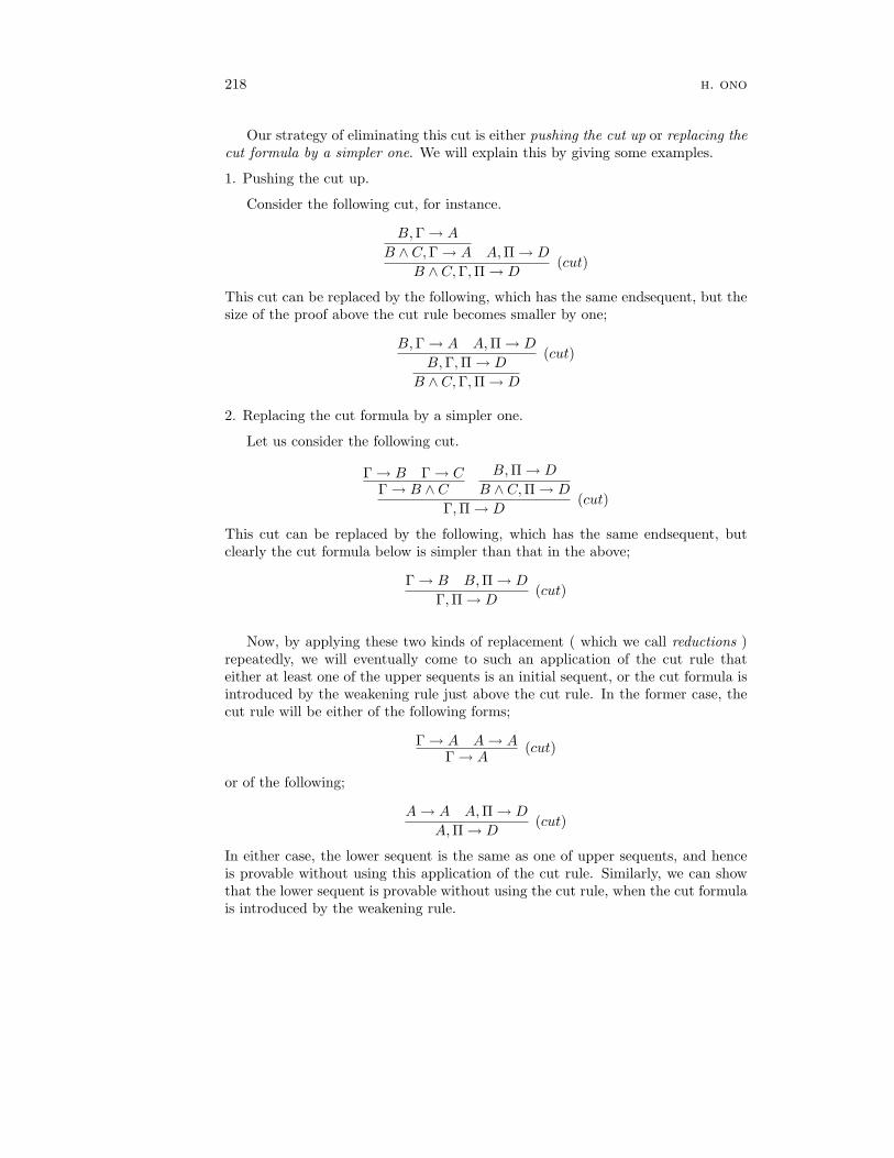
Our strategy of eliminating this cut is either pushing the cut up or replacing thecut formula by a simpler one. We will explain this by giving some examples.

1. Pushing the cut up.

Consider the following cut, for instance.

B, Γ → A

B ∧ C, Γ → A A, Π → D

B ∧ C, Γ, Π → D(cut)

This cut can be replaced by the following, which has the same endsequent, but thesize of the proof above the cut rule becomes smaller by one;

B, Γ → A A, Π → D

B, Γ, Π → D(cut)

B ∧ C, Γ, Π → D

2. Replacing the cut formula by a simpler one.

Let us consider the following cut.

Γ → B Γ → CΓ → B ∧ C

B, Π → D

B ∧ C, Π → D

Γ, Π → D(cut)

This cut can be replaced by the following, which has the same endsequent, butclearly the cut formula below is simpler than that in the above;

Γ → B B, Π → D

Γ, Π → D(cut)

Now, by applying these two kinds of replacement ( which we call reductions )repeatedly, we will eventually come to such an application of the cut rule thateither at least one of the upper sequents is an initial sequent, or the cut formula isintroduced by the weakening rule just above the cut rule. In the former case, thecut rule will be either of the following forms;

Γ → A A → AΓ → A

(cut)

or of the following;

A → A A, Π → D

A, Π → D(cut)

In either case, the lower sequent is the same as one of upper sequents, and henceis provable without using this application of the cut rule. Similarly, we can showthat the lower sequent is provable without using the cut rule, when the cut formulais introduced by the weakening rule.


So far, so good. But, there is only one case where the above reduction does notwork. This is caused by the contraction rule. In fact, consider the following cut;

Γ → A

A,A, Π → D

A, Π → D(c →)

Γ, Π → D(cut)

One may reduce this to;

Γ → A

Γ → A A,A, Π → D

A, Γ, Π → D(cut)

Γ, Γ, Π → D(cut)

Γ, Π → Dsome(e →)(c →)

Here, while the size of the proof above the upper application of the cut rule becomessmaller, the one above the lower application will not. Thus, some modifications ofthe present idea will be necessary.

3.2 Mix rule

To overcome the above difficulty, Gentzen took the following modified form ofthe cut rule, called the mix rule, instead of the cut rule.

Mix rule:

Γ → A, Θ Π → ∆

Γ, ΠA → ∆, ΘA(mix)

,

where Π has at least one occurrence of A, and both ΠA and ΘA are sequences offormulas obtained from Π and Θ, respectively, by deleting all occurrences of A.( For LJ, we assume that Θ is empty and ∆ consists of at most one formula. ) Wecall the formula A, the mix formula of the above application of the mix rule.

Let LK† and LJ† be sequent calculi obtained from LK and LJ by replacingthe cut rule by the mix rule. We can show the following.

Lemma 3 For any sequent S, S is provable in LK† ( LJ† ) if and only if it isprovable in LK ( LJ, respectively ).

Proof. We will show this for LJ† and LJ. To show this, it is enough to prove thatthe cut rule is derivable in LJ† and conversely that the mix rule is derivable in LJ.First, consider the following cut;

Γ → A A, Π → D

Γ, Π → D

Then, the following figure shows that this cut is derivable in LJ†:

220 h. ono

Γ → A A, Π → D

Γ, ΠA → D(mix)

Γ, Π → Dsome(w →)

Conversely, take the following mix;

Γ → A Π → ∆Γ, ΠA → D

Then, this mix is derivable in LJ, as the following figure shows.

Γ → AΠ → D

A, ΠA → Dsome(c →)(e →)

Γ, ΠA → D(cut)

Now, we will return back once again to the beginning. So, we suppose thata proof P of a sequent S in LJ is given. By using the way in the proof of theabove Lemma, we can get a proof Q of a sequent S in LJ†, which may containsome applications of the mix rule, but no applications of the cut rule. This time,we will try to eliminate applications of the mix rule inductively, by taking oneof uppermost applications of the mix rule in Q. Each reduction introduced in theprevious subsection works completely well after this modification. In particular,

Γ → A

A,A, Π → D

A, Π → D(c →)

Γ, ΠA → D(mix)

will be reduced to;

Γ → A A,A, Π → D

Γ, ΠA → D(mix)

Clearly, the size of the latter proof becomes smaller than that of the former. But,the replacement of the cut rule by the mix rule forces us to introduce a new notionof the “simplicity” of a proof. To see this, let us consider the following applicationof the mix rule, where we assume that A ∧ B doesn’t occur in Γ.

Γ → A ∧ B

A,B → D

A,A ∧ B → D

A ∧ B,A ∧ B → D

Γ → D(mix)

The above application of the mix rule can be replaced by the following;


Γ → A ∧ B

Γ → A ∧ B

A,B → D

A,A ∧ B → D

A, Γ → D(mix)

A ∧ B, Γ → D

Γ, Γ → D(mix)

Γ → Dsome(c →)(e →)

It is easy to see that the size of the proof above the lower application of the mixrule becomes greater than before. Hence, we need to introduce the notion of therank, instead of the size, to measure the simplicity of the proof. Roughly speaking,the rank of a given application of the mix rule with the mix formula C is definedas follows. We consider such branches in a given proof that start from a sequentS which contains an occurrence of C in the succedent and ends at the left uppersequent of this mix. ( The occurrence of C in S must be an ancestor of the mixformula C. ) The left rank r1 of this mix rule is the maximal length of thesebranches. Similarly, the right rank r2 is the maximal length of branches which endat the right upper sequent of this mix. Then, we call the sum r1 + r2, the rank ofthis mix rule. ( As for the precise definition of the rank, see [43]. )

In the above case, the right rank r2 of the mix rule is 2 in the upper proof. Onthe other hand, both of the right ranks of the two applications of the mix rule are1 in the lower proof, while all of the left ranks are the same.

What remains to show is whether the procedure described in the above willeventually terminate. For a given formula A, define the grade of A by the numberof occurrences of logical connectives in it. Take one of uppermost applications ofthe mix rule in a given Q. Define the grade of this application of the mix by thegrade of its mix formula.

Then, we can show that after any of these reductions, either the grade becomessmaller, or the rank becomes smaller while the grade remains the same. Thus,by using the double induction on the grade and the rank, we can derive that eachuppermost application of the mix is eliminable. This completes the proof of themix elimination theorem of LJ†. So, we have a proof R of S in LJ† without anyapplication of the mix rule. It is obvious that R can be regarded as a proof of Sin LJ without any application of the cut rule. Thus, we have the cut eliminationtheorem for LJ.

3.3 Cut elimination theorem for nonclassical logics

By modifying the proof of the cut elimination theorem for LK and LJ in theprevious subsection, we can get the cut elimination theorem for some importantnonclassical logics. For sequent calculi for modal logics introduced in Section 2, wehave the following.

Theorem 4 The cut elimination theorem holds for GK, GKT and GS4.

222 h. ono

On the other hand, the cut elimination theorem doesn’t hold for GS5, as thefollowing Lemma shows.

Lemma 5 The sequent p → 2¬2¬p is provable in GS5, but is not provable inGS5 without applying the cut rule.

Proof. The following is a proof of p → 2¬2¬p in GS5.

2¬p → 2¬p→ ¬2¬p,2¬p→ 2¬2¬p,2¬p

p → p¬p, p →

2¬p, p →p → 2¬2¬p (cut)

Now, suppose that p → 2¬2¬p has a cut-free proof. Then, consider the lastinference in the proof. By checking the list of rules of inference of GS5 ( exceptthe cut rule, of course ), we can see that only the weakening rule and the contractionrule are possible. By repeating this, we can see that this cut-free proof containsonly sequents of the form, p → , → 2¬2¬p and p, . . . , p → 2¬2¬p, . . . ,2¬2¬p.Thus, it can never contain any initial sequent. This is a contradiction.

For basic substructural logics, we have the following.

Theorem 6 Cut elimination holds for FL, FLe, FLw, FLew, FLec, and FLecw.It holds also for CFLe, CFLew, CFLec and CFLecw.

We will give here some remarks on Theorem 6. As the discussions in 3.1 show,it suffices for us to show the cut elimination theorem ( not the mix eliminationtheorem ) directly for basic substructural logics without the contraction rule, i.e.FL, FLe, FLw, FLew, CFLe and CFLew, by using double induction on the gradeand the length. For, the source of obstacles in proving the cut elimination theoremdirectly is the contraction rule.

Next, consider substructural logics FLec and CFLec, each of which has boththe exchange and the contraction rules, but not the weakening rule. As we haveshown in 3.2 ( see the proof of Lemma 3 ), we need both the weakening and thecontraction rules, to replace the cut by the mix rule. But, this difficulty can beovercome by introducing a generalized form of the mix rule. For example, thegeneralized form of the mix rule for FLec is given as follows;

Γ → A Π → C

Γ, ΠA → C(g − mix)

where Π has at least one occurrence of A, and ΠA is a sequence of formulas obtainedfrom Π by deleting at least one occurrence of A.

This replacement of the cut rule by the generalized mix rule works well onlywhen we have the exchange rule. In fact, we have the following.


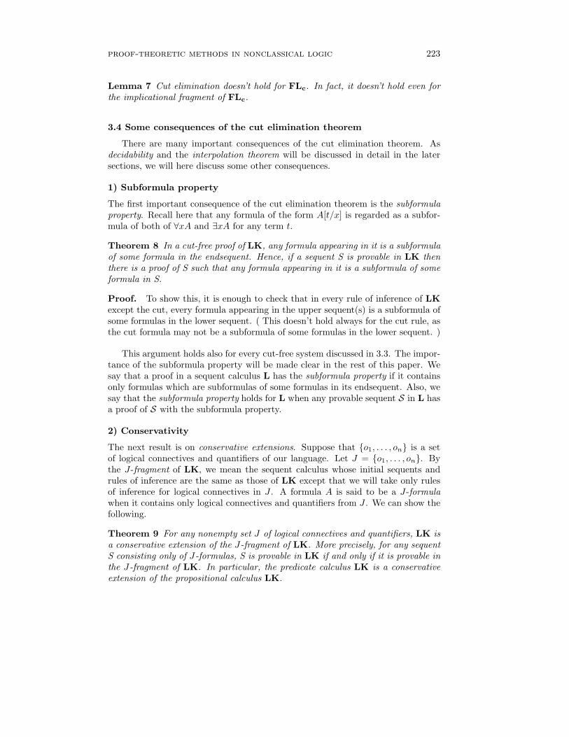
Lemma 7 Cut elimination doesn’t hold for FLc. In fact, it doesn’t hold even forthe implicational fragment of FLc.

3.4 Some consequences of the cut elimination theorem

There are many important consequences of the cut elimination theorem. Asdecidability and the interpolation theorem will be discussed in detail in the latersections, we will here discuss some other consequences.

1) Subformula property

The first important consequence of the cut elimination theorem is the subformulaproperty. Recall here that any formula of the form A[t/x] is regarded as a subfor-mula of both of ∀xA and ∃xA for any term t.

Theorem 8 In a cut-free proof of LK, any formula appearing in it is a subformulaof some formula in the endsequent. Hence, if a sequent S is provable in LK thenthere is a proof of S such that any formula appearing in it is a subformula of someformula in S.

Proof. To show this, it is enough to check that in every rule of inference of LKexcept the cut, every formula appearing in the upper sequent(s) is a subformula ofsome formulas in the lower sequent. ( This doesn’t hold always for the cut rule, asthe cut formula may not be a subformula of some formulas in the lower sequent. )

This argument holds also for every cut-free system discussed in 3.3. The impor-tance of the subformula property will be made clear in the rest of this paper. Wesay that a proof in a sequent calculus L has the subformula property if it containsonly formulas which are subformulas of some formulas in its endsequent. Also, wesay that the subformula property holds for L when any provable sequent S in L hasa proof of S with the subformula property.

2) Conservativity

The next result is on conservative extensions. Suppose that {o1, . . . , on} is a setof logical connectives and quantifiers of our language. Let J = {o1, . . . , on}. Bythe J-fragment of LK, we mean the sequent calculus whose initial sequents andrules of inference are the same as those of LK except that we will take only rulesof inference for logical connectives in J . A formula A is said to be a J-formulawhen it contains only logical connectives and quantifiers from J . We can show thefollowing.

Theorem 9 For any nonempty set J of logical connectives and quantifiers, LK isa conservative extension of the J-fragment of LK. More precisely, for any sequentS consisting only of J-formulas, S is provable in LK if and only if it is provable inthe J-fragment of LK. In particular, the predicate calculus LK is a conservativeextension of the propositional calculus LK.

224 h. ono

Proof. The if-part of the Theorem is trivial. So suppose that a sequent S whichconsists only of J-formulas is provable in LK. Consider a cut-free proof P of S inLK. By the subformula property of LK, P contains only J-formulas. Then we cansee that there is no chance of applying a rule of inference for a logical connectiveor a quantifier other than those from J . Thus, P can be regarded as a proof in theJ-fragment of LK.

By this theorem, it becomes unnecessary to say in which fragment of LK agiven sequent is provable, as long as it is provable in LK. It is easy to see thatthis theorem holds for any other system as long as the subformula property holdsfor it.

3) Disjunction property

A logic L has the disjunction property when for any formulas A and B, if A∨B isprovable in L then either A or B is provable in it. Classical logic doesn’t have thedisjunction property, as p ∨ ¬p is provable but neither of p and ¬p are provable.On the other hand, the following holds.

Theorem 10 Intuitionistic logic has the disjunction property.

Proof. Suppose that the sequent → A ∨ B is provable in LJ. It suffices to showthat either → A or → B is provable in it. Consider any cut-free proof P of → A∨B.Then the last inference in P will be either (→ w) or (→ ∨). If it is (→ w) thenthe upper sequent must be → . But this is impossible. Hence, it must be (→ ∨).Then the upper sequent is either → A or → B. This completes the proof.

By using the similar argument, we have the following.

Theorem 11 Each of FL, FLe, FLw, FLew and FLec has the disjunction prop-erty.

As mentioned before, classical logic doesn’t have the disjunction property. Then,where does the above argument break for classical logic? The answer may be ob-tained easily by checking the proof of → p ∨ ¬p in LK. In this case, the lastinference is (→ c). This suggests that we can use the same argument as in theabove when we have no contraction rules. Thus, we have the following result, inaddition.

Theorem 12 Both CFLe and CFLew have the disjunction property.

An immediate consequence of the above theorem is that the sequent → p ∨ ¬pis not provable in CFLew. Note that CFLew is obtained from FLew by adding¬¬A → A as additional initial sequents. On the other hand, the system obtainedfrom FLew by adding → A ∨ ¬A as initial sequents becomes classical logic.

In the same way as in LK, we can show that CFLec doesn’t have the disjunctionproperty. On the other hand, we note that the presence of the contraction rule


(→ c) doesn’t cause always the failure of the disjunction property. For instance,consider the sequent calculus LJ′ for the intuitionistic logic, which is obtainedfrom LK by restricting (→ ¬), (→⊃) and (→ ∀) to those for LJ. Though LJ′ is acut-free system with (→ c), it has still the disjunction property.

3.5 Subformula property revisited

As shown in the above, the cut elimination theorem doesn’t hold for the sequentcalculus GS5. On the other hand, we can show the following.

Theorem 13 The sequent calculus GS5 has the subformula property.

To show this, we will introduce the notion of acceptable cuts, which sometimesare called analytic cuts, as follows. An application of the following cut rule isacceptable

Γ → A, Θ A, Π → ∆

Γ, Π → Θ, ∆

if the cut formula A is a subformula of a formula in Γ, Θ, Π, ∆.

Then, we can show the following result, from which Theorem 13 follows imme-diately.

Theorem 14 For any sequent S, if S is provable in GS5, then there exists a proofof S in GS5 such that every application of the cut rule in it is acceptable.

Note that the proof of p → 2¬2¬p given in the proof of Lemma 5 containsan application of the cut rule, but it is an acceptable one. To show the theorem,we need to eliminate each non-acceptable application of the cut rule. This can bedone in the same way as the proof of the cut elimination theorem. Similar resultsholds also for some other modal logics.

The importance of this result lies in the fact that most consequences of thecut elimination theorem are obtained from the subformula property. Thus, we canrephrase this fact in the following way: The most important proof-theoretic propertyis the subformula property, and the most convenient way of showing the subformulaproperty is to show the cut elimination theorem.

3.6 Notes

To get the detailed information on the proof of the cut elimination theoremand on the consequences of it, both [43] and [45] will be useful. The result ofLemma 5 was noticed by Ohnishi and Matsumoto in their joint paper 1959. Severalpeople including S. Kanger, G. Mints, M. Sato, M. Ohnishi etc., introduced cut-freesystems for S5.

Theorem 6 is shown in [35] and [32]. A generalized form of the mix rule wasintroduced in the paper [23]. On the other hand, the negative result on FLc isdiscussed in [4]. The subformula property for GS5 and the related systems are

226 h. ono

discussed in Takano’s paper [42]. The proof is based on a deep proof-theoreticanalysis. Recently, he succeeded to extend his method to some intuitionistic modallogics, i.e. modal logics based on the intuitionistic logic. Related results are ob-tained by Fitting [15, 16], in which semantical methods are used. Further study inthis direction seems to be promising.

4 Decision Problems for the Classical and the In-

tuitionistic Logics

In this and the next sections, we will discuss decision problems of various logics.A given logic L is said to be decidable if there exists an algorithm that can decidewhether a formula A is provable in L or not, for any A. It is undecidable if it is notdecidable. The decision problem of a given logic L is the problem as to whether Lis decidable or not. In this section, we will show the decidability of classical andintuitionistic propositional logics as a consequence of the cut elimination theoremfor propositional calculi for both LK and LJ by using Gentzen’s method. Inthe next section, we will show that most of basic substructural logics withoutthe contraction rule are decidable even if they are predicate logics. On the otherhand, we can show that a certain complication will occur in decision problems forsubstructural logics with the contraction rule but without the weakening rule.

4.1 Basic ideas of proving decidability

We will explain here a method of checking the provability of a given sequent inpropositional LK, which is due to Gentzen. The decision algorithm for proposi-tional LJ can be obtained similarly. Suppose that a sequent Γ → ∆ is given. Wewill try to search for a proof of this sequent. If we succeed to find one, Γ → ∆ isof course provable, and if we fail, then it is not provable. But, as there may beinfinitely many possible proofs of it, how can we know that we have failed?

Thus, it is necessary to see whether we can restrict the range of search ofproofs, hopefully to finitely many proofs, or not. Now let us consider the followingrestrictions on proofs.1) Proofs with the subformula property, in particular cut-free proofs: For LK, thisis possible, since we have the cut elimination theorem for LK. Thus, if Γ → ∆ isprovable in LK then there must exist a ( cut-free ) proof such that any sequent init consists only of formulas which are subformulas of some formulas in Γ → ∆.2) Proofs with no redundancies: Here, we say that a proof P has redundancies if thesame sequent appears twice in a branch of P. Every proof having some redundanciescan be transformed into one with no redundancies. In fact, a redundancy of Σ → Πin the following proof


P0

Σ → Π...

Σ → ΠP1

Γ → ∆

can be eliminated as follow;

P0

Σ → ΠP1

Γ → ∆.

But, the above two conditions are not enough to reduce the number of allpossible proofs to finitely many. To see this, suppose that a given sequent D, Λ → Θsatisfies the condition that it consists only of subformulas of some formulas in

Γ → ∆. Then, any sequent of the form

n︷︸︸︷

D, . . . ,D, Λ → Θ also satisfies this forany natural number n.

Thus we need to add an additional condition. A sequent Σ → Π is reducedif every formula in it occurs at most three times in the antecedent and also atmost three times in the succedent. In particular, we say that a sequent Σ → Π is1-reduced if every formula in the antecedent ( the succedent ) occurs exactly oncein the antecedent ( the succedent, respectively ).

A sequent Γ† → ∆† is called a contraction of a sequent Γ → ∆ if it is obtainedfrom Γ → ∆ by applying the contraction and exchange rule repeatedly. For in-stance, the sequent A,C → B is a contraction of a sequent A,C,A,A → B. Now,we can show easily that for any given sequent Γ → ∆, there exists a ( 1- )reducedsequent Γ∗ → ∆∗, which is a contraction of Γ → ∆, such that Γ → ∆ is provablein LK if and only if Γ∗ → ∆∗ is provable in LK. In fact, if a formula C appearsmore than three times either in Γ or in ∆ then we can reduce the number of oc-currences of C to three ( or, even to one ) by applying the contraction rule ( andthe exchange rule, if necessary ) repeatedly. In this way, we can get a ( 1- )reducedsequent Γ∗ → ∆∗. Conversely, by applying the weakening rule to Γ∗ → ∆∗ asmany times as necessary, we can recover Γ → ∆. Thus, there exists an effectiveway of getting a ( 1- )reduced sequent S ′ for a given sequent S, whose provability isthe same as that of S. So, it suffices to get an algorithm which can decide whethera given reduced sequent is provable or not. We have the following.

Lemma 15 Suppose that Γ → ∆ is a sequent which is provable in LK and thatΓ∗ → ∆∗ is any 1-reduced contraction of Γ → ∆. Then, there exists a cut-freeproof of Γ∗ → ∆∗ in LK such that every sequent appearing in it is reduced.

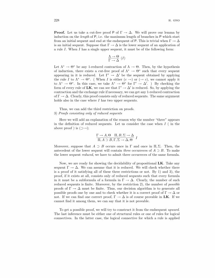
228 h. ono

Proof. Let us take a cut-free proof P of Γ → ∆. We will prove our lemma byinduction on the length of P, i.e. the maximum length of branches in P which startfrom an initial sequent and end at the endsequent of P. This is trivial when Γ → ∆is an initial sequent. Suppose that Γ → ∆ is the lower sequent of an application ofa rule I. When I has a single upper sequent, it must be of the following form:

Λ → ΘΓ → ∆

(I)

Let Λ∗ → Θ∗ be any 1-reduced contraction of Λ → Θ. Then, by the hypothesisof induction, there exists a cut-free proof of Λ∗ → Θ∗ such that every sequentappearing in it is reduced. Let Γ′ → ∆′ be the sequent obtained by applyingthe rule I to Λ∗ → Θ∗. ( When I is either (c →) or (→ c), we cannot apply itto Λ∗ → Θ∗. In this case, we take Λ∗ → Θ∗ for Γ′ → ∆′. ) By checking theform of every rule of LK, we can see that Γ′ → ∆′ is reduced. So, by applying thecontraction and the exchange rule if necessary, we can get any 1-reduced contractionof Γ → ∆. Clearly, this proof consists only of reduced sequents. The same argumentholds also in the case where I has two upper sequents.

Thus, we can add the third restriction on proofs.3) Proofs consisting only of reduced sequents

Here we will add an explanation of the reason why the number “three” appearsin the definition of reduced sequents. Let us consider the case when I ( in theabove proof ) is (⊃→);

Γ → A, Θ Π, B, Σ → ∆

Π, A ⊃ B, Γ, Σ → ∆, ΘI

Moreover, suppose that A ⊃ B occurs once in Γ and once in Π, Σ. Then, theantecedent of the lower sequent will contain three occurreces of A ⊃ B. To makethe lower sequent reduced, we have to admit three occurreces of the same formula.

Now, we are ready for showing the decidability of propositional LK. Take anysequent Γ → ∆. We can assume that it is reduced. We will check whether thereis a proof of it satisfying all of these three restrictions or not. By 1) and 3), theproof, if it exists at all, consists only of reduced sequents such that every formulain it must be a subformula of a formula in Γ → ∆. Clearly, the number of suchreduced sequents is finite. Moreover, by the restriction 2), the number of possibleproofs of Γ → ∆ must be finite. Thus, our decision algorithm is to generate allpossible proofs one by one and to check whether it is a correct proof of Γ → ∆ ornot. If we can find one correct proof, Γ → ∆ is of course provable in LK. If wecannot find it among them, we can say that it is not provable.

To get a possible proof, we will try to construct it from the endsequent upward.The last inference must be either one of structural rules or one of rules for logicalconnectives. In the latter case, the logical connective for which a rule is applied


must be an outermost logical connective of a formula in the endsequent. Therefore,there are finitely many possiblities. We will repeat this again for sequents whichare obtained already in this way. Note that a possible proof will branch upward, ingeneral, and therefore it is necessary to continue the above construction to the topof each branch. When we reach a sequent which doesn’t produce any new sequent,we will check whether it is an initial sequent or not. If we can find at least onenon-initial sequent among them, we fail. This procedure is sometimes called, theproof-search algorithm. Thus, we have the following

Theorem 16 Both classical and intuitionistic propositional logics are decidable.

Here are two examples of possible proofs of → p ∨ (p ⊃ q). The left one is afailed one and the right one is a correct proof.

p → q→ p ⊃ q (→⊃)

→ p ∨ (p ⊃ q)(→ ∨2)

p → pp → p, q (→ w)

→ p, p ⊃ q (→⊃)

→ p, p ∨ (p ⊃ q)(→ ∨2)

→ p ∨ (p ⊃ q), p ∨ (p ⊃ q)(→ ∨1)

→ p ∨ (p ⊃ q)(→ c)

For modal logics introduced in Section 2, we can use essentially the same deci-sion procedure as that for LK and therefore have the following.

Theorem 17 Any of modal propositional logics K, KT, S4 and S5 is decidable.

Note that here the subformula property, but not the cut elimination theorem,is essential in the proof of the decidability mentioned above. Thus, the decidabilityof S5 follows from Theorem 13.

4.2 Digression — a simplified decision algorithm for the classical propo-sitional logic

In the previous subsection, we have given an algorithm which decides the prov-ability of a given sequent S in LK. Moreover, the algorithm gives us a cut-free proofof S when it is provable. But the algorithm contains a thorough search of proofssatisfying certain conditions and thus needs trial and error. For propositional LK,we can give a simpler decision algorithm, as shown below. This algorithm mightbe quite instructive, when one learns how to construct a cut-free proof of a givensequent if it is provable.

On the other hand, for practical purposes a lot of work has been done onefficient algorithms of deciding whether a given sequent is provable in LK or not,or equivalently whether a given formula is tautology or not.

For a given sequent S, define decompositions of S as follows. Any decompositionis either a sequent or an expression of the form 〈S1;S2〉 for some sequents S1 andS2.

230 h. ono

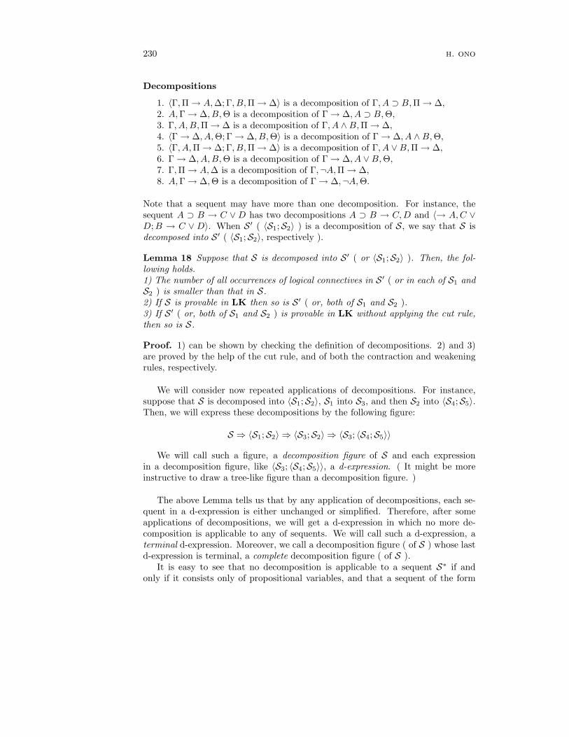
Decompositions

1. 〈Γ, Π → A, ∆; Γ, B, Π → ∆〉 is a decomposition of Γ, A ⊃ B, Π → ∆,2. A, Γ → ∆, B, Θ is a decomposition of Γ → ∆, A ⊃ B, Θ,3. Γ, A,B, Π → ∆ is a decomposition of Γ, A ∧ B, Π → ∆,4. 〈Γ → ∆, A, Θ; Γ → ∆, B, Θ〉 is a decomposition of Γ → ∆, A ∧ B, Θ,5. 〈Γ, A, Π → ∆; Γ, B, Π → ∆〉 is a decomposition of Γ, A ∨ B, Π → ∆,6. Γ → ∆, A,B, Θ is a decomposition of Γ → ∆, A ∨ B, Θ,7. Γ, Π → A, ∆ is a decomposition of Γ,¬A, Π → ∆,8. A, Γ → ∆, Θ is a decomposition of Γ → ∆,¬A, Θ.

Note that a sequent may have more than one decomposition. For instance, thesequent A ⊃ B → C ∨ D has two decompositions A ⊃ B → C,D and 〈→ A,C ∨D; B → C ∨ D〉. When S ′ ( 〈S1;S2〉 ) is a decomposition of S, we say that S isdecomposed into S ′ ( 〈S1;S2〉, respectively ).

Lemma 18 Suppose that S is decomposed into S ′ ( or 〈S1;S2〉 ). Then, the fol-lowing holds.1) The number of all occurrences of logical connectives in S ′ ( or in each of S1 andS2 ) is smaller than that in S.2) If S is provable in LK then so is S ′ ( or, both of S1 and S2 ).3) If S ′ ( or, both of S1 and S2 ) is provable in LK without applying the cut rule,then so is S.

Proof. 1) can be shown by checking the definition of decompositions. 2) and 3)are proved by the help of the cut rule, and of both the contraction and weakeningrules, respectively.

We will consider now repeated applications of decompositions. For instance,suppose that S is decomposed into 〈S1;S2〉, S1 into S3, and then S2 into 〈S4;S5〉.Then, we will express these decompositions by the following figure:

S ⇒ 〈S1;S2〉 ⇒ 〈S3;S2〉 ⇒ 〈S3; 〈S4;S5〉〉

We will call such a figure, a decomposition figure of S and each expressionin a decomposition figure, like 〈S3; 〈S4;S5〉〉, a d-expression. ( It might be moreinstructive to draw a tree-like figure than a decomposition figure. )

The above Lemma tells us that by any application of decompositions, each se-quent in a d-expression is either unchanged or simplified. Therefore, after someapplications of decompositions, we will get a d-expression in which no more de-composition is applicable to any of sequents. We will call such a d-expression, aterminal d-expression. Moreover, we call a decomposition figure ( of S ) whose lastd-expression is terminal, a complete decomposition figure ( of S ).

It is easy to see that no decomposition is applicable to a sequent S∗ if andonly if it consists only of propositional variables, and that a sequent of the form


p1, . . . , pm → q1, . . . , qn with propositional variables p1, . . . , pm, q1, . . . , qn is prov-able in LK if and only if pi is identical with qj for some i ( ≤ m ) and j ( ≤ n ).

Now, take an arbitrary sequent S and take any one of its complete decomposi-tion D. Then, by Lemma 18 2) and 3), S is provable if and only if every sequent inthe terminal d-expression of D is provable. We can decide whether the latter holdsor not, by checking whether every sequent has a common propositional variablein the antecedent and the succedent or not. This gives us a decision algorithmfor classical propositional logic. We note here that the present algorithm doesn’tcontain any trial and error.

Furthermore, when every sequent in the terminal d-expression of D is provable,we can construct a cut-free proof of S effectively from D by supplementing someapplications of the contraction and the weakening rules. Here is an example. Con-sider the sequent → ((p ⊃ q) ⊃ p) ⊃ p. The following is a complete decompositionfigure of it.

→ ((p ⊃ q) ⊃ p) ⊃ p ⇒ (p ⊃ q) ⊃ p → p ⇒ 〈→ p, p ⊃ q; p → p〉 ⇒ 〈p → p, q; p → p〉

Since each of p → p, q and p → p has a common propositional variable in theantecedent and the succedent, the above sequent must be provable in LK. In fact,it has a cut-free proof shown below, which obtained from the above decompositionfigure by supplementing some contraction and weakening rules.

p → pp → p, q (→ w)

→ p, p ⊃ q p → p

(p ⊃ q) ⊃ p → p, p

(p ⊃ q) ⊃ p → p(→ c)

→ ((p ⊃ q) ⊃ p) ⊃ p

The above argument will suggest us an alternative sequent calculus for theclassical propositional logic, which we call LK∗. Sequents of LK∗ are expressionsof the form Γ → ∆, where both Γ and ∆ are finite multisets of formulas. Initialsequents of LK∗ are sequents of the form A, Γ → ∆, A. LK∗ has no structuralrules and no cut rule. It has only the following rules for logical connectives.

Rules for logical connectives of LK∗:

Γ → ∆, A B, Γ → ∆

A ⊃ B, Γ → ∆(⊃→)

A, Γ → ∆, B

Γ → ∆, A ⊃ B(→⊃)

A,B, Γ → ∆

A ∧ B, Γ → ∆(∧ →)

Γ → ∆, A Γ → ∆, B

Γ → ∆, A ∧ B(→ ∧)

A, Γ → ∆ B, Γ → ∆

A ∨ B, Γ → ∆(∨ →)

Γ → ∆, A,B

Γ → ∆, A ∨ B(→ ∨)

232 h. ono

Γ → ∆, A

¬A, Γ → ∆(¬ →)

A, Γ → ∆

Γ → ∆,¬A(→ ¬)

From the above argument, the following result follows immediately. ( Here, wewill neglect the difference of the definition of sequents in these two systems forbrevity. )

Theorem 19 For any sequent S, S is provable in LK∗ if and only if it is provablein LK.

4.3 Undecidability of the classical and the intuitionistic predicate logics

A. Church proved the following in 1936.

Theorem 20 The classical predicate logic is undecidable.

It may be helpful to point out where the decision procedure mentioned in theprevious subsection breaks for the predicate LK. This will be understood bylooking at rules (∀ →) and (→ ∃) for quantifiers. In these rules, corresponding toa formula of the form ∀xA or ∃xA in the lower sequent, a formula A[t/x], which isa subformula ( in a broad sense ) of ∀xA or ∃xA, appears in the upper sequent forsome term t. But, this t may not appear in the lower sequent, in general. Thus, itbecomes necessary to search for an appropriate t.

When our language L contains no function symbols, a term in L is eitheran individual variable or an individual constant. Even in this case, we can-not resolve the above difficulty. For instance, a proof of a sequent of the form∀xA, Σ → Π following the above three restrictions contain reduced sequents of theform A[u1/x], . . . , A[un/x], Λ → Θ for some n, where each ui is either an individualvariable or an individual constant. Thus, the number of reduced sequents will beinfinite.

Define a mapping α on the set of first-order formulas of L inductively, as follows.

α(A) = ¬¬A if A is an atomic formula,α(A ∧ B) = α(A) ∧ α(B), α(A ⊃ B) = α(A) ⊃ α(B),α(¬A) = ¬α(A), α(A ∨ B) = ¬(¬α(A) ∧ ¬α(B)),α(∀xA) = ∀xα(A), α(∃xA) = ¬∀x¬α(A).

We can show the following.

Lemma 21 For any first-order formula A, A is provable in LK if and only if α(A)is provable in LJ.

Proof. It is easy to see that α(A) ⊃ A is provable in LK for any A. Thus, the if-part of the Lemma follows. We can show that ¬¬α(A) ⊃ α(A) is provable in LJ forany A. Moreover by using induction, we can show that if a sequent A1, . . . , Am →B1, . . . , Bn is provable in LK then α(A1), . . . , α(Am),¬α(B1), . . . ,¬α(Bn) → is


provable in LJ. Thus, if A is provable in LK then ¬¬α(A) and hence α(A) areprovable in LJ.

By Theorem 20 and Lemma 21, we have the following.

Theorem 22 The intuitionistic predicate logic is undecidable.

Proof. Suppose otherwise. Let us take an arbitrary formula A and calculate α(A).( This calculation is carried out effectively. ) By using the decision algorithm for theintuitionistic predicate logic, we check whether α(A) is provable in the intuitionisticpredicate logic or not. Then, by Lemma 21 this enables us to see whether A isprovable in the classical predicate logic or not. But, this contradicts Theorem 20.

4.4 Notes

The decision algorithm mentioned in 4.1 is based on the result by Gentzen [17].See also [43]. In implementing these algorithms by computers, it becomes necessaryto consider their efficiency. Thus, such an approach as one in 4.2 may be useful.As for efficient decision algorithms for intuitionistic logic, see also Notes 5.4 in thenext section. As for the details of the proof of Theorem 20, see e.g. [14].

5 Decision Problems for Substructural Logics

5.1 Decidability of substructural logics without the contraction rule

Next, we will discuss the decision problems for basic substructural logics. Itwill be natural to start by checking whether our decision algorithm mentionedin the previous section can be applied to the present case or not. Since the cutelimination theorem holds for all basic substructural logics but FLc, we can limitthe range of possible proofs to those with the subformula property and of course,with no redundancies. On the other hand, our discussion on reduced sequents, inparticular the proof of Lemma 15, relies on the presence of both the contractionand the weakening rules. Here, some modifications or new ideas will be necessary.

First, we will consider basic substructural logics without the contraction rule.In this case, no essential difficulties will occur, and in fact the decision algorithmwill be much easier than that of LK and LJ. This follows from the followingobservation. Let us look at every rule of inference in the propositional LK or LJexcept the cut and the contraction rules. Then, we can see easily that in any ofsuch rules ( either of ) its upper sequent(s) is simpler than the lower sequent. Thus,the number of sequents which can appear in a cut-free proof of a given sequent isfinite, and hence the number of possible sequents is also finite. Thus, we havethe decidability of basic substructural propositional logics without the contractionrule.

234 h. ono

This argument can be easily extended to the predicate logics, when our languagecontains neither function symbols nor individual constants. Consider rules foruniversal quantifiers:

Γ, A[t/x], Σ → ∆

Γ,∀xA, Σ → ∆(∀ →)

Γ → Λ, A[z/x], Θ

Γ → Λ,∀xA, Θ(→ ∀)

In our proof-search algorithm, we must find a suitable upper sequent for a givenlower sequent. In the case of (→ ∀), for z, we will take the first individual variablenot appearing in the lower sequent, assuming an enumeration of all individualvariables at the beginning. In the present case, the term t in (∀ →) must be anindividual variable. We can show that as a possible upper sequent, it is enoughto consider the sequent of the form Γ, A[t/x], Σ → ∆ such that t is either one offree variables appearing in the lower sequent or the first individual variable notappearing in the lower sequent. ( In fact, if t is a new variable, we replace it bythe first new variable, which doesn’t affect its provability. ) Rules for existentialquantifiers can be treated in the same way.

Now, consider the proof-search for a given sequent S. Let y1, . . . , yk be all thefree variables in S. For the sake of convenience, we assume that y1, . . . , yk comeas the first k individual variables in our enumeration of all individual variables.Let m be the number of all quantifiers in S and put n = k + m. Then, by theabove argument, we can see that it is enough to consider sequents consisting ofsubformulas of formulas in S whose free individual variables are among the firstn variables in the enumeration. This implies that the number of such sequents isfinite. Therefore, we have shown the decidability of basic substructural predicatelogics without the contraction rule, provided that the language contains neitherfunction symbols nor individual constants. Though we will not go into the details,we can extend the decidability result for them, even if our language contains bothfunction symbols and individual constants. ( see [23] for details ).

Theorem 23 Any of the substructural predicate logics FL, FLe, FLw, FLew,CFLe and CFLew ( with function symbols and individual constants ) is decidable.

5.2 Decision problems for substructural propositional logics with thecontraction rule

Next we will consider decision problems for substructural logics FLec andCFLec. We will discuss only the decision problem for FLec in detail, as the case forCFLec can be treated similarly. The arguments in this and the next subsectionswill be more technical than the previous ones. So, readers may skip the deatails ofthe proofs in their first reading and may look only at the results.

First, we will start from the propositional FLec. As we have shown in theprevious subsection, the main troubles in decision problems were caused by thecontraction rule. In our proof-search for a given sequent S, we must consider thecase where it is obtained from sequents, which are more complicated than S, by


applying the contraction rule many times. As we have already shown, when wehave moreover the weakening rule, with the help of reduced sequents we can provethat the number of possible proofs is finite. But, we cannot use reduced sequentsin general.

To overcome this difficulty, we will remove the contraction rule from the systemFLec and instead of this, modify each rule for logical connectives into one whichcontains implicit applications of the contraction rule. We will call the system thusobtained, FLec

′. In order to avoid making the present paper too technical, wewill not give the full details of the system FLec

′ here, but introduce only its im-plicational fragment to explain the idea. By our definition, sequents of FLec areexpressions of the form Γ → C with a ( possibly empty ) sequence Γ of formulasand a ( possibly empty ) formula C. On the other hand, sequents of FLec

′ areexpressions of the form Γ → C with a ( possibly empty ) finite multiset Γ of for-mulas and a ( possibly empty ) formula C. ( This is only for the sake of brevity.In this way, we can dispense with the exchange rule. ) The system FLec

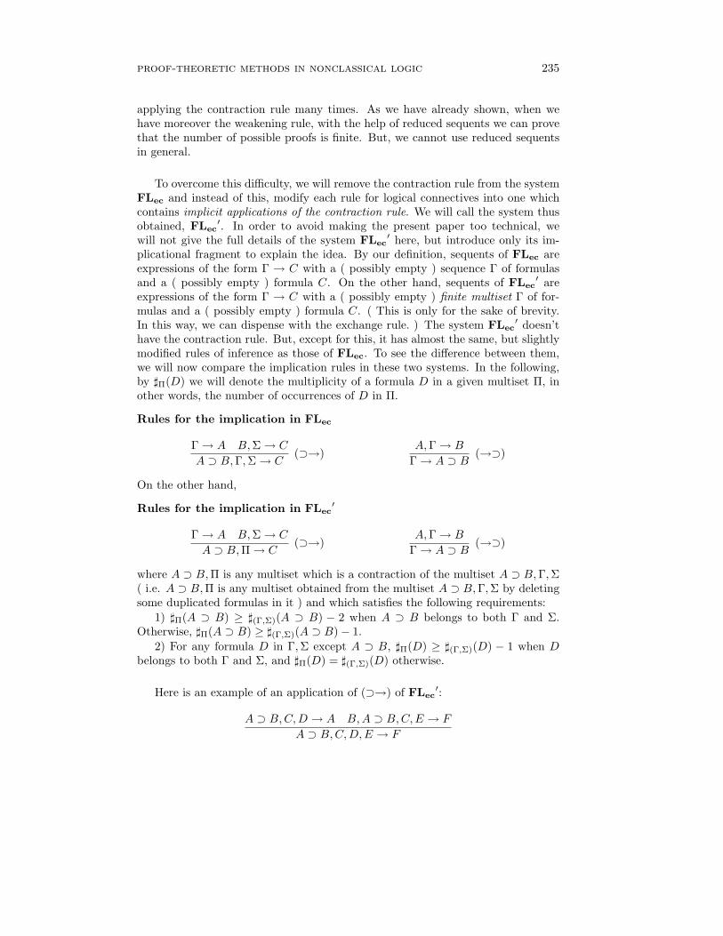
′ doesn’thave the contraction rule. But, except for this, it has almost the same, but slightlymodified rules of inference as those of FLec. To see the difference between them,we will now compare the implication rules in these two systems. In the following,by ♯Π(D) we will denote the multiplicity of a formula D in a given multiset Π, inother words, the number of occurrences of D in Π.

Rules for the implication in FLec

Γ → A B, Σ → C

A ⊃ B, Γ, Σ → C(⊃→)

A, Γ → B

Γ → A ⊃ B(→⊃)

On the other hand,

Rules for the implication in FLec′

Γ → A B, Σ → C

A ⊃ B, Π → C(⊃→)

A, Γ → B

Γ → A ⊃ B(→⊃)

where A ⊃ B, Π is any multiset which is a contraction of the multiset A ⊃ B, Γ, Σ( i.e. A ⊃ B, Π is any multiset obtained from the multiset A ⊃ B, Γ, Σ by deletingsome duplicated formulas in it ) and which satisfies the following requirements:

1) ♯Π(A ⊃ B) ≥ ♯(Γ,Σ)(A ⊃ B) − 2 when A ⊃ B belongs to both Γ and Σ.Otherwise, ♯Π(A ⊃ B) ≥ ♯(Γ,Σ)(A ⊃ B) − 1.

2) For any formula D in Γ, Σ except A ⊃ B, ♯Π(D) ≥ ♯(Γ,Σ)(D) − 1 when Dbelongs to both Γ and Σ, and ♯Π(D) = ♯(Γ,Σ)(D) otherwise.

Here is an example of an application of (⊃→) of FLec′:

A ⊃ B,C,D → A B,A ⊃ B,C,E → F

A ⊃ B,C,D,E → F

236 h. ono

Note that there is some freedom of the choice of Π. We can show that the cutelimination theorem holds for FLec

′ and that for any formula A, A is provable inFLec

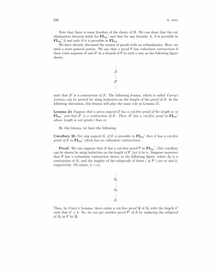
′ if and only if it is provable in FLec.We have already discussed the notion of proofs with no redundancies. Here, we

need a more general notion. We say that a proof P has redundant contractions ifthere exist sequents S and S ′ in a branch of P in such a way as the following figureshows;

...S...S ′

...

such that S ′ is a contraction of S. The following lemma, which is called Curry’sLemma, can be proved by using induction on the length of the proof of S. In thefollowing discussion, this lemma will play the same role as Lemma 15.

Lemma 24 Suppose that a given sequent S has a cut-free proof of the length m inFLec

′ and that S ′ is a contraction of S. Then, S ′ has a cut-free proof in FLec′

whose length is not greater than m.

By this lemma, we have the following.

Corollary 25 For any sequent S, if S is provable in FLec′ then it has a cut-free

proof of S in FLec′ which has no redundant contractions.

Proof. We can suppose that S has a cut-free proof P in FLec′. Our corollary

can be shown by using induction on the length of P. Let it be n. Suppose moreoverthat P has a redundant contraction shown in the following figure, where S2 is acontraction of S1 and the lengths of the subproofs of them ( in P ) are m and k,respectively. Of course, k < m.

...S1...S2...S.

Then, by Curry’s Lemma, there exists a cut-free proof Q of S2 with the length k′

such that k′ ≤ k. So, we can get another proof P’ of S by replacing the subproofof S2 in P by Q,


Q

S2...S

with the length n′ such that n′ < n, since k′ ≤ k < m. Hence, by the hypothesisof induction we can get a proof of S with no redundant contractions.

5.3 Termination of the proof-search algorithm

Here, we will look over our situation again. In the present case, we cannot limitthe number of sequents in possible proofs to be finite. What we can assume nowis that we can restrict our attention only to proofs with the subformula propertyand what is more, to proofs with no redundant contractions. Then, are these tworestrictions on possible proofs enough to make the total number of possible proofsfinite? This is not so obvious. Let us consider the following example. Here, we willwrite the sequence A, . . . , A with n occurrences of A as An. For a given sequentS which is A3, B2, C5 → D, take three sequents A4, B,C4 → D, A2, B3, C4 → Dand A5, B2, C3 → D. Then, S is not a contraction of any of them. Moreover, anyone of them is not a contraction of any other. Thus, all of them may appear in thesame branch of a possible proof of S with no redundant contractions. So, we willface the following combinatorial problem.

Suppose that formulas A1, . . . , Am,D are given. Consider a sequence 〈S1,S2,. . .〉 of sequents such that each member is always of the form A1

k1 , . . . , Amkm → D,

where each ki is positive. ( Any sequence of this kind is sometimes called a sequenceof cognate sequents. ) Moreover, assume that Si is not a contraction of Sj wheneveri < j. Our question is; can such a sequence be of infinite length? Or, is the lengthof such a sequence always finite? ( Note that the replacement of the condition“whenever i < j” by “whenever i 6= j” doesn’t affect the answer, since the numberof sequents which are contractions of a given Si is obviously finite. )

This problem is mathematically the same as the following. Let N be the set ofall positive integers, and Nm be the set of all n-tuples (k1, . . . , km) such that ki ∈ Nfor each i. Define a binary relation ≤∗ on Nm by (k1, . . . , km) ≤∗ (h1, . . . , hm) ifand only if ki ≤ hi for each i. Clearly, ≤∗ is a partial order. A subset W of Nm iscalled an antichain if for any distinct u, v ∈ W neither u ≤∗ v nor v ≤∗ u hold.Then, are there infinite antichains of Nm? The answer is negative.

Lemma 26 Any antichain of Nm is finite.

This result can be proved by various ways. One way is to show the followinglemma, from which the above lemma follows immediately. A partial order � on agiven set Y is well-founded if there are no descending chains in Y , i.e. there areno elements {si}i∈N in Y such that si+1 ≺ si for each i. A partial order � on agiven set Y is a well partial order if it is well-founded and moreover Y contains noinfinite antichain with respect to �.

238 h. ono

Lemma 27 1) The natural order on N is a well partial order.2) Suppose that both sets U and V have well partial orders ≤1 and ≤2, respectively.Then, their direct product order ≤ on U × V is also a well partial order. Here, ≤is defined by (u, v) ≤ (u′, v′) if and only if u ≤1 u′ and v ≤2 v′.

Corollary 28 Suppose that 〈S1,S2, . . .〉 is a sequence of cognate sequents such thatSi is not a contraction of Sj whenever i < j. Then, it is finite.

This result is known under the name of Kripke’s Lemma. Now, let us considerthe following “complete proof-search tree” of a given sequent S. Take any sequentor any pair of sequents from which S follows by a single application of a rule ofinference ( except the cut rule, of course ). Write any of them just over S as longas it consists only of subformulas of formulas in S. We will regard each of themas an immediate predecessor of S. Then, repeat this again for each immediatepredecessors, and continue this as long as possible. If a sequent is initial, it hasno immediate predecessors. Also, when a sequent thus generated has a contractionbelow it, we will not add it in the tree.

Then, it is easy to see that if S is provable then there exists a proof which formsa subtree of the “complete proof-search tree” of S. We can see that the number ofthe branching at each “node” of the complete proof-search tree is finite, since eachsequent has only finitely many, possible upper sequents. Furthermore, the length ofeach branch in the complete proof-search tree is finite by Kripke’s Lemma. Thus,the complete proof-search tree of any S is finite, by the following lemma, calledKonig’s Lemma.

Lemma 29 A tree is finite if and only if the number of the branching at each nodeof the tree is finite and the length of each branch in the tree is finite.

Thus, it turns out that a given sequent S is provable if and only if there exists aproof of S which is a subtree of its complete proof-search tree. Since the completeproof-search tree is finite, we can check whether it contains a proof of S or not.Now we have the following.

Theorem 30 Substructural propositional logics FLec and CFLec are decidable.

On the other hand, the same difficulties as the classical predicate logic occur inthe decision problems of predicate logics FLec and CFLec. In fact, we can showthe following.

Theorem 31 Substructural predicate logics FLec and CFLec are undecidable.

5.4 Notes

In 5.2, we have explained a way of incorporating the contraction rule into rulesfor logical connectives and as a result, of eliminating the explicit contraction rule.A similar idea can be applied to intuitionistic propositional logic. But, the systemstill contains some circularities in the proof-search, caused by the rule (⊃→). By


dividing it into several rules, it is possible to remove these circularities and hence,we can get an efficient decision algorithm for intuitionistic propositional logic. Thiswas done independently by Hudelmaier and Dyckhoff. See [21] and [13]. See also[40].

The fact that even predicate logics will be decidable when they have no contrac-tion rules was mentioned already at the beginning of sixties by H. Wang. As forthe details of proofs in 5.1, see [24] and [23]. On the other hand, the idea of provingthe decidability of propositional logic with the contraction rule was first introducedby S. Kripke in 1959 and then is extended to CFLec by R.K. Meyer in his disserta-tion of 1966. See also [12] and [23]. Lemma 27 2) is attributed to G. Higman. Formore information on the lemma and the related topics, see e.g. [25]. Our decisionalgorithm for logics with the contraction rule relies on Kripke’s Lemma which isquite nonconstructive, and hence it is quite probable that the computational com-plexity of the algorithm will be high. Obviously, adding the distributive law willmake the situation worse. In fact, in 1984 A. Urquhart showed the undecidablityof ( even the positive fragment of ) the relevant propositional logic R, which isequivalent to the system CFLec with the distributive law. ( See [46]. ) Restall in[39] obtained the decidability of some substructural logics using the proof theorybased on display calculi. A survey of decision problems of substructural logics isgiven in [34].

6 Interpolation Property

W. Craig proved in 1957 the following result, now called Craig’s interpolationtheorem for classical logic. In the following, V (D) denotes the set of all predicatesymbols in a formula D. ( Thus, V (D) denotes the set of all propositional variablesin D when we are concerned with propositional logic. ) When Γ is a sequence offormulas D1, . . . ,Dm, we define V (Γ) = V (D1) ∪ . . . ∪ V (Dm).

Theorem 32 If a formula A ⊃ B is provable in classical logic then there existsa formula C such that both A ⊃ C and C ⊃ B are provable, and that V (C) ⊆V (A) ∩ V (B).

Any formula C satisfying the conditions in the above theorem is called, aninterpolant of A ⊃ B. Precisely speaking, the above statement contains a certaininaccuracy as it doesn’t mention the case when the set V (A)∩V (B) is empty. For,when our language L doesn’t contain any predicate ( or propositional ) constant,there is no formula C with V (C) ⊆ V (A) ∩ V (B). As a matter of fact, the abovetheorem holds even for the case when V (C) ⊆ V (A) ∩ V (B) if L contains oneof ⊤ and ⊥. On the other hand, when it has neither predicate nor propositionalconstants at all, we have to add the following.

When V (A) ∩ V (B) is empty, either ¬A or B is provable.

240 h. ono

We will return back to this problem again later. The same result holds also forintuitionistic logic. Craig’s interpolation theorem is known to be equivalent toBeth’s definability theorem and also to Robinson’s consistency theorem. ( See e.g.[9] for the details, in which the equivalence is shown by using model-theoreticmethods. )

We say that a logic L has the interpolation property if the statement in the abovetheorem holds for L. For intermediate propositional logics, i.e. propositional logicsbetween intuitionistic logic and classical, L. Maksimova proved in 1977 the followingstriking result, which we mentioned already in the Introduction, by reducing it tothe amalgamation property of varieties of Heyting algebras. Note here that thereare uncountably many intermediate propositional logics.

Theorem 33 Only seven intermediate propositional logics have the interpolationproperty.

She proved also a similar theorem for modal propositional logics which arenormal extensions of S4.

6.1 Maehara’s method

There are various ways of proving the interpolation property. Craig obtainedthe theorem by using semantical methods. In 1960, S. Maehara showed that Craig’sinterpolation theorem for classical logic follows from the cut elimination theoremfor LK. Different from semantical methods, the proof by Maehara’s method willgive us a concrete form of an interpolant of a formula A ⊃ B, once a cut-free proofof A ⊃ B is given.

In the following, we will explain Maehara’s method for intuitionistic logic andthen for other nonclassical logics. Let LJ◦ be the sequent calculus obtained fromLJ by adding the following initial sequents for propositional constants ⊤ and ⊥(see subsection 2.3):

1. → ⊤2. ⊥ →

It is easy to see that the cut elimination theorem holds also for LJ◦ and hence thatit is a conservative extension of LJ. For any given finite sequence Γ of formulas,we call a pair 〈Γ1; Γ2〉 of ( possibly empty ) sequences of formulas Γ1 and Γ2, apartition of Γ, if the mutiset union of Γ1 and Γ2 is equal to Γ when regarding Γ, Γ1

and Γ2 as multisets of formulas. Now, we will show the following.

Lemma 34 Suppose that a sequent Γ → ∆ is provable in LJ◦ and that 〈Γ1; Γ2〉is any partition of Γ. Then, there exists a formula C such that both Γ1 → C andC, Γ2 → ∆ are provable in LJ◦, and moreover that V (C) ⊆ V (Γ1) ∩ V (Γ2, ∆).

Proof. Let us also call such a formula C, an interpolant of Γ → ∆ ( with respectto the partition 〈Γ1; Γ2〉 ). Since the cut elimination theorem holds for LJ◦, we cantake a cut-free proof P of Γ → ∆. We will prove our theorem by induction on the


length n of P. Suppose that n = 1. In this case, Γ → ∆ must be an initital sequent.Let it be A → A. It is necessary to consider two partitions of A, i.e. 〈A; ∅〉 and〈∅; A〉. For the former case, we can take A itself for an interpolant. For the lattercase, we can take ⊤ for an interpolant, as both sequents → ⊤ and ⊤, A → A areprovable. Similarly, we can show the existence of an interpolant for both → ⊤ and⊥ → with respect to any partition.

Next suppose that n > 1. Let I be the last rule of inference in P. By thehypothesis of induction, we can assume that there exists an interpolant of ( eachof ) the upper sequent(s) of I with respect to an arbitrary partition. It is necessaryto show that the lower sequent Γ → ∆ has also an interpolant with respect to anypartition. We need to check this for any rule of inference of LJ◦. In the following,we will show this only when I is either (∨ →) or (→ ∨).

1) Suppose that Γ is A ∨ B, Γ′ and that I is an application of (∨ →) as follow;

A, Γ′ → ∆ B, Γ′ → ∆

A ∨ B, Γ′ → ∆

1.1) Consider a partition 〈A∨B, Γ1; Γ2〉 of A∨B, Γ′. Taking a partition 〈A, Γ1; Γ2〉of A, Γ′ and a partition 〈B, Γ1; Γ2〉 of B, Γ′ and using the hypothesis of induction,we can get formulas C and D such that

(1a) both A, Γ1 → C and C, Γ2 → ∆ are provable(1b) V (C) ⊆ V (A, Γ1) ∩ V (Γ2, ∆)(2a) both B, Γ1 → D and D, Γ2 → ∆ are provable(2b) V (D) ⊆ V (B, Γ1) ∩ V (Γ2, ∆)

Then, by (1a) and (2a) we have that both A∨B, Γ1 → C∨D and C∨D, Γ2 → ∆ areprovable, and moreover by (1b) and (2b) that V (C∨D) ⊆ V (A∨B, Γ1)∩V (Γ2, ∆).Hence, the formula C ∨ D is an interpolant.

1.2) Next, consider a partition 〈Γ1; A ∨ B, Γ2〉 of A ∨ B, Γ′. This time, we takea partition 〈Γ1; A, Γ2〉 of A, Γ′ and a partition 〈Γ1; B, Γ2〉 of B, Γ′. Then, by thehypothesis of induction, we can get formulas C and D such that

(3a) both Γ1 → C and C,A, Γ2 → ∆ are provable(3b) V (C) ⊆ V (Γ1) ∩ V (A, Γ2, ∆)(4a) both Γ1 → D and D,B, Γ2 → ∆ are provable(4b) V (D) ⊆ V (Γ1) ∩ V (B, Γ2, ∆)

It follows that both Γ1 → C ∧ D and C ∧ D,A ∨ B, Γ2 → ∆ are provable, andthat V (C ∧ D) ⊆ V (Γ1) ∩ V (A ∨ B, Γ2, ∆). Therefore, the formula C ∧ D is aninterpolant in this case.

2) Suppose next that I is an application of (→ ∨1) as follows:

Γ → AΓ → A ∨ B

Let 〈Γ1; Γ2〉 be any partition of Γ. By the hypothesis of induction, there exists aformula C such that

(5a) both Γ1 → C and C, Γ2 → A are provable

242 h. ono

(5b) V (C) ⊆ V (Γ1) ∩ V (Γ2, A)Then, clearly both Γ1 → C and C, Γ2 → A ∨ B are provable, and it holds thatV (C) ⊆ V (Γ1) ∩ V (Γ2, A ∨ B). Hence, the formula C is an interpolant. In thesame way, we can treat the case (→ ∨2).

In Lemma 34, take A → B for Γ → ∆ and consider the partition 〈A; ∅〉 of A.Then, we can show Craig’s interpolation theorem for intuitionistic logic.

Theorem 35 If a sequent A → B is provable in LJ◦ then there exists a formulaC such that both A → C and C → B are provable in LJ◦, and moreover thatV (C) ⊆ V (A) ∩ V (B).

Maehara’s method can be applied also to classical logic. In this case, we needto modify the definition of partitions as follows, as sequents in LK are of the formΓ → ∆ where both Γ and ∆ are arbitrary finite sequences of formulas. Supposethat a sequent Γ → ∆ is given. Suppose moreover that the mutiset union of Γ1 andΓ2 ( ∆1 and ∆2 ) is equal to Γ ( ∆, respectively ) as multisets of formulas. Thenwe say that 〈(Γ1 : ∆1); (Γ2 : ∆2)〉 is a partition of Γ → ∆. Instead of Lemma 34,we show the following lemma, where the sequent calculus LK◦ is an extension ofLK, obtained in the same way as LJ◦.

Lemma 36 Suppose that a sequent Γ → ∆ is provable in LK◦ and that 〈(Γ1 :∆1); (Γ2 : ∆2)〉 is any partition of Γ → ∆. Then, there exists a formula C suchthat both Γ1 → ∆1, C and C, Γ2 → ∆2 are provable in LK◦, and moreover thatV (C) ⊆ V (Γ1, ∆1) ∩ V (Γ2, ∆2).

Now, Craig’s interpolation theorem for classical logic follows immediately fromthe above lemma.

Theorem 37 If a sequent A → B is provable in LK◦ then there exists a formulaC such that both A → C and C → B are provable in LK◦, and moreover thatV (C) ⊆ V (A) ∩ V (B).

We note here that the reason why we need to consider arbitrary partitions inLemmas 34 and 36 comes from forms of rules for implication and negation. Forinstance, consider the following (→⊃):

p ∧ r, p ⊃ q → q ∨ s

p ∧ r → (p ⊃ q) ⊃ (q ∨ s)

In this case, though q is an interpolant of the upper sequent, it isn’t an interpolantof the lower sequent. An interpolant of the lower sequent is p. Thus, if we don’tconsider interpolants corresponding to each partition, the proof using inductionwill break down here.

6.2 Eliminating constants


Consider any interpolant C given in Theorems 35 and 37. When it containspropositional constants ⊤ and ⊥, we can simplify the formula C by using thefollowing logical equivalence. Here, A ∼ B means that A is logically equivalent toB in LJ.

(1) ⊤ ⊃ E ∼ E, ⊥ ⊃ E ∼ ⊤, E ⊃ ⊤ ∼ ⊤, E ⊃ ⊥ ∼ ¬E,(2) ⊤ ∧ E ∼ E, ⊥ ∧ E ∼ ⊥,(3) ⊤ ∨ E ∼ ⊤, ⊥ ∨ E ∼ E,(4) ¬⊤ ∼ ⊥, ¬⊥ ∼ ⊤.

By repeating this simplification, C will be transformed into a formula C ′ which iseither a formula without any propositional constant, or a propositional constantitself. In the former case, we get an interpolant with no propositional constants.

Let us consider the latter case. First, suppose that the set V (A) ∩ V (B) isnonempty in Theorem 35 or in Theorem 37. Then, C ′ is logically equivalent toeither F ⊃ F or ¬(F ⊃ F ), where F is an arbitrary formula consisting only ofpredicate symbols ( or propositional variables ) in V (A) ∩ V (B). Hence, we canget an interpolant with no propositional constants also in this case.

But when the set V (A) ∩ V (B) is empty, we cannot get such an interpolant.Let us suppose that C ′ is ⊤. In this case, A → ⊤ and ⊤ → B are provable. But,the first one is always provable, and the second is provable if and only if → B isprovable. Suppose next that C ′ is ⊥. Then, A → ⊥ and ⊥ → B are provable. Thesecond sequent is always provable, and the first is provable if and only if A → isprovable. Thus, we have the following.

Theorem 38 Suppose that a formula A ⊃ B is provable in LK. If the set V (A)∩V (B) is nonempty, there exists a formula C such that both A ⊃ C and C ⊃ B areprovable in LK and V (C) ⊆ V (A) ∩ V (B). If the set V (A) ∩ V (B) is empty, theneither ¬A or B is provable in LK. This holds also for LJ.

We note here that Craig’s interpolation theorem for classical and intuitionisticlogic doesn’t necessarily imply the theorem for fragments of them. In fact, ourproof of Lemma 34 shows that a conjunctive formula C ∧ D is needed in the case1.2) where the rule of inference is for the disjunction.

6.3 Digression — least and greatest interpolants

Consider Craig’s interpolation theorem of the form of Theorem 38. It is easy tosee that interpolants of A ⊃ B are not always determined uniquely ( up to logicalequivalence ). For instance, consider the following formula which is provable in LJ;

(p ∧ (p ⊃ (r ∧ s))) ⊃ (q ⊃ (r ∨ s)).

We can see that all of formulas r ∧ s, r, s and r ∨ s are interpolants of the aboveformula.

We say that an interpolant C of a formula A ⊃ B is least if C ⊃ D is provablefor any interpolant D of a formula A ⊃ B, and is greatest if D ⊃ C is provable

244 h. ono

for any interpolant D of a formula A ⊃ B. In the above case, we can show thatr ∧ s and r ∨ s are least and greatest interpolants, respectively. In fact, we havethe following.

Theorem 39 Suppose that A ⊃ B is a formula provable in the propositional LKand that the set V (A)∩V (B) is nonempty. Then, there exist both least and greatestinterpolants of A ⊃ B ( in LK ).

Proof. To show our Theorem, we will use an elementary semantical method. Infact, the proof in the following will give an alternative proof of Craig’s interpolationtheorem for classical propositional logic. First, we recall an elementary fact thatany formula A ⊃ B is provable in the classical propositional logic if and only ifit is a tautology, i.e. for any valuation f , f(A ⊃ B) = t. Here, a valuation is amapping from the set of propositional variables ( occurring in the formula underconsideration ) to the set of truth values { t, f }. Let U ( and V ) be the setV (A)\V (B) ( and the set V (B)\V (A), respectively ). Let us take an arbitrarypropositional variable s ∈ V (A) ∩ V (B) and fix it.

Now, take any valuation f with the domain U . Let Af be the formula obtainedfrom A by replacing each variable p ∈ U by s ⊃ s if f(p) = t and by ¬(s ⊃ s),otherwise. ( Of course, you may simplify Af by using the logical equivalence. )Define A∗ to be the formula

∨

fAf , where f runs over all valuations with thedomain U . Similarly, we define the formula Bg for any valuation g with the domainV . Then, define B∗ to be the formula

∧

gBg, where g runs over all valuations withthe domain V .

We will show that A∗ and B∗ are least and greatest interpolants, respectively, ofthe formula A ⊃ B. First, it is easily seen that both V (A∗) and V (B∗) are subsetsof V (A)∩V (B). Suppose that h is an arbitrary valuation with the domain V (A) andh′ is the restriction of h to the domain U . Clearly, h(A) = h(Ah′) holds. Therefore,if h(A) = t then h(Ah′) = t and hence h(A∗) = t. Thus, A ⊃ A∗ is a tautology.Next, let f and j be arbitrary valuations with the domain U and the domain V (B),respectively. Since U and V (B) are disjoint, we can define a valuation fj with thedomain V (A)∪V (B) by fj(p) = f(p) if p ∈ U , and fj(p) = j(p) if p ∈ V (B). SinceA ⊃ B is a tautology, fj(A ⊃ B) = t for any such j. Since the restriction of fj

to U is f , fj(A) = fj(Af ) = j(Af ). Thus, fj(A ⊃ B) = j(Af ⊃ B). Hence, theformula Af ⊃ B is a tautology, and therefore is provable in classical logic, for anyf with the domain U . Hence, A∗ ⊃ B, which is

∨

fAf ⊃ B by the definition, isprovable. Thus, we have shown that A∗ is an interpolant. To show that it is least,assume that C is any interpolant. Obviously, A ⊃ C is a tautology. Thus, by usingthe same argument as mentioned just in the above, we can infer that A∗ ⊃ C isprovable. Thus, A∗ is least. Similarly, we can show that B∗ is greatest.

The above proof depends on the fact that a given formula is provable in classicalpropositional logic if and only if it is a tautology. Thus, it will be hard to applythe present method to other logics. On the other hand, A.M. Pitts succeeded inshowing that the similar result holds for intuitionistic propositional logic, by usinghighly technical, proof-theoretic methods.


Theorem 40 Suppose that A ⊃ B is a formula provable in propositional LJ andthat the set V (A) ∩ V (B) is nonempty. Then, there exist both least and greatestinterpolants of A ⊃ B ( in LJ ).

6.4 Interpolation theorem for modal logics

We can apply Maehara’s method to modal logics discussed in Section 3. Thereare two points, of which we should be careful. The first one is to eliminate propo-sitional constants. In the modal logic K, 2⊤ is logically equivalent to ⊤, and⊥ ⊃ 2⊥ is provable. But, 2⊥ ⊃ ⊥ ( or equivalently, 3⊤ ) is not provable. Thus,K ( with propositional constants ) has the interpolation property of the form ofTheorem 37, but doesn’t have the interpolation property of the form of Theorem 38.On the other hand, when a modal logic has the axiom scheme T , i.e. 2A ⊃ A, 2⊥becomes logically equivalent to ⊥ in it, and hence we can eliminate propositionalconstants by using the method mentioned in 6.2.

The second point is that what is needed in applying Maehara’s method is notthe cut elimination theorem, but the subformula property. Thus, we can show thatCraig’s interpolation theorem holds for S5. In the following, we will explain thedetails. Let us consider the following acceptable cut rule.

Γ → Θ, A A, Π → ∆

Γ, Π → Θ, ∆

Take any partition 〈(Γ1, Π1 : Θ1, ∆1); (Γ2, Π2 : Θ2, ∆2)〉 of Γ, Π → Θ, ∆. Wewill show that there exists an interpolant E such that both Γ1, Π1 → Θ1, ∆1, Eand E, Γ2, Π2 → Θ2, ∆2 are provable in S5, and V (E) ⊆ V (Γ1, Π1, Θ1, ∆1) ∩V (Γ2, Π2, Θ2, ∆2).

1) Suppose that A is one of the subformulas of a formula in Γ2, Π2, Θ2, ∆2. Letus take the partition 〈(Γ1 : Θ1); (Γ2 : Θ2, A)〉 of Γ → Θ, A, and the partition〈(Π1 : ∆1); (A, Π2 : ∆2)〉 of A, Π → ∆. Then, by the hypothesis of induction, thereexist formulas C and D such that

(1a) both Γ1 → Θ1, C and C, Γ2 → Θ2, A are provable,(1b) V (C) ⊆ V (Γ1, Θ1) ∩ V (Γ2, Θ2, A),(2a) both Π1 → ∆1,D and A,D, Π2 → ∆2 are provable,(2b) V (D) ⊆ V (Π1, ∆1) ∩ V (A, Π2, ∆2).

By using the first sequents of (1a) and (2a), the sequent Γ1, Π1 → Θ1, ∆1, C ∧D isshown to be provable. Next, by applying the cut rule to the second sequents of (1a)and (2a) ( with the cut formula A ), the sequent C,D, Γ2, Π2 → Θ2, ∆2, and henceC ∧D, Γ2, Π2 → Θ2, ∆2 are shown to be provable. Moreover, V (C ∧D) ⊆ (V (C)∪V (D)) ⊆ (V (Γ1, Π1, Θ1, ∆1)∩V (Γ2, Π2, Θ2, ∆2)), since V (A) ⊆ V (Γ2, Π2, Θ2, ∆2).Thus, C ∧ D is an interpolant.

2) Suppose otherwise. That is, A is not a subformula of any formula in Γ2, Π2, Θ2,∆2. In this case, A must be a subformula of a formula in Γ1, Π1, Θ1, ∆1. Take thepartition 〈(Γ1 : Θ1, A); (Γ2 : Θ2)〉 of Γ → Θ, A, and the partition 〈(A, Π1 : ∆1);

246 h. ono

(Π2 : ∆2)〉 of A, Π → ∆. Then, the hypothesis of induction, there exist formulasF and G such that

(3a) both Γ1 → Θ1, A, F and F, Γ2 → Θ2 are provable,(3b) V (F ) ⊆ V (Γ1, Θ1, A) ∩ V (Γ2, Θ2),(4a) both A, Π1 → ∆1, G and G, Π2 → ∆2 are provable,(4b) V (G) ⊆ V (A, Π1, ∆1) ∩ V (Π2, ∆2).

By applying the cut rule to the first sequents of (3a) and (4a) with the cut formulaA, we get the sequent Γ1, Π1 → Θ1, ∆1, F ∨G. Also, by taking the second sequentsof (3a) and (4a), and applying the weakening rules and (∨ →), we get the sequentF ∨G, Γ2, Π2 → Θ2, ∆2. Moreover, using both (3b) and (4b), we can see that F ∨Gis an interpolant. Hence, we have the following.

Theorem 41 Craig’s interpolation theorem holds for any of the modal proposi-tional logics K, KT, S4 and S5.

6.5 Interpolation theorem for substructural logics

Next, consider the interpolation theorem for substructural logics. We will takethe formulation of sequent calculi for basic substructural logics given in Section 2.First, suppose that our language contains propositional constants. Then, similarlyto the classical and the intuitionistic cases, we can show the following, by usingMaehara’s method.

Theorem 42 Craig’s interpolation theorem holds for substructural logics FL, FLw,FLe, FLew, FLec, CFLe, CFLew and CFLec ( in the language with proposi-tional constants ).

We notice that the above theorem holds for both propositional and predicatelogics. To show the theorem for substructural logics without the exchange rule,like FL and FLw, we need to modify the definition of partitions in the followingway. Let Γ → ∆ be any sequent ( of FL, or FLw ). Then, a triple 〈Γ1; Γ2; Γ3〉 is apartition of Γ, if the sequence Γ1, Γ2, Γ3 is equal to Γ ( without changing the orderof formulas ). Then, Theorem 42 follows by showing the following.

Lemma 43 Suppose that a sequent Γ → ∆ is provable in FL ( and FLw ) andthat 〈Γ1; Γ2; Γ3〉 is any partition of Γ. Then, there exists a formula C such thatboth Γ2 → C and Γ1, C, Γ3 → ∆ are provable in FL ( and FLw, respectively ),and moreover that V (C) ⊆ V (Γ2) ∩ V (Γ1, Γ3, ∆).

As we mentioned in 2.3, it is enough to consider two propositional constants ⊤and ⊥ when a given logic has the weakening rule. Moreover, the following logicalequivalences hold in FLw for the logical connective ∗; for any formula E,

⊤ ∗ E ∼ E, E ∗ ⊤ ∼ E, ⊥ ∗ E ∼ ⊥, E ∗ ⊥ ∼ ⊥.Thus, by using the method discussed in 6.2, we can eliminate propositional con-stants. Let FLw

′ be the sequent calculus in the propositional language withoutpropositional constants, obtained from FLw by deleting all initial sequents forpropositional constants and rules of inference for them.


Corollary 44 Suppose that a formula A ⊃ B is provable in FLw′. If the set

V (A) ∩ V (B) is nonempty, there exists a formula C such that both A ⊃ C andC ⊃ B are provable in FLw

′, and V (C) ⊆ V (A) ∩ V (B). If the set V (A) ∩ V (B)is empty, then either ¬A or B is provable in FLw

′. This holds also for the calculiFLew and CFLew without propositional constants.

On the other hand, we cannot eliminate propositional constants always in otherlogics mentioned in Theorem 42. But, as shown in Section 7, when the set V (A)∩V (B) is empty, the formula A ⊃ B is never provable in these basic substructural(predicate) logics without the weakening rule.

6.6 Notes

For the details of a proof of Craig’s interpolation theorem for classical logicby Maehara’s method, see e.g. [43]. Theorem 33 and the related result on modallogics are shown by Maksimova in [27] and [28], respectively.

Theorem 40 by Pitts is given in [36], in which he took a sequent calculus forintuitionistic propositional logic, introduced independently by Hudelmaier and Dy-ckhoff. ( See Notes 5.4. ) A proof of the interpolation theorem for modal logicS5 based on the subformula property of the sequent calculus GS5 is mentioned in[42]. A general result on the interpolation theorem for modal logics formulated intableau calculi is given by Rautenberg [38].

Interpolation theorems for various substructural logics are discussed in [35] andalso in [32]. Recently, Bayu Surarso succeeded to extend Maehara’s method andproved the interpolation theorem for many distributive substructural logics ( see[3] ).

7 Variable Sharing and Variable Separation

We will add two more examples from the study of substructural logics which showthe usefulness of proof-theoretic methods. The first one is the variable sharingproperty which is known for some relevant logics. The second one is Maksimova’sprinciple of variable separation. We can see that the weakening rule plays animportant role in them.

7.1 Variable sharing property of substructural logics without the weak-ening rule

We say that a logic L has the variable sharing property, when for any formulaA ⊃ B without propositional constants, if A ⊃ B is provable in L then V (A) ∩V (B) is nonempty. It is clear by the definition that if a logic L has the variablesharing property and L′ is weaker than L ( i.e. every fromula provable in L′ is alsoprovable in L ), then L′ has also the property. In [1], it is shown that the relevantpropositional logic R has the variable sharing property.

248 h. ono

Theorem 45 The predicate logic CFLec has the variable sharing property, and afortiori any of FL, FLe, FLec and CFLe has the variable sharing property.

We will give here a proof of the above theorem for FLec. The proof for CFLec

can be shown essentially in the same way. Recall that every sequent in FLec isof the form Π → Λ, where Λ contains at most one formula. To show the abovetheorem, it is enough to prove the following.

Theorem 46 Suppose that Γ → A is a sequent containing no propositional con-stants such that Γ is nonempty. If Γ → A is provable in FLec then V (Γ) ∩ V (A)is nonempty.

Proof. Suppose that Γ → A satisfies the conditions in the theorem and is provablein FLec. Then, it has a cut-free proof P. Clearly, P contains neither initial sequentsfor propositional constants nor rules for propositional constants. We will show thatthere exists a branch in P starting from an initial sequent and ending at the sequentΓ → A such that every sequent Π → Λ in the branch contains at least two formulas,i.e. either both of Π and Λ are nonempty, or Λ is empty but Π contains at leasttwo formulas. Of course, Γ → A contains at least two formulas. For other sequentsin P, we will show this by checking that for any rule of inference of FLec, if thelower sequent contains at least two formulas then ( at least one of ) the uppersequent(s) contains at least two formulas. ( For rules (⊃→) and (→ ∗), one of theupper sequents may not contain two formulas. Of course, the above doesn’t holdin general when we have the weakening rule. )

Now, let B be any such branch. For any sequent Π → Λ containing at least twoformulas, we say that 〈Π1; Π2, Λ〉 is a partition of Π → Λ if the multiset union ofΠ1 and Π2 is equal to Π, and both Π1 and Π2, Λ are nonempty. By our assumptionon Π → Λ, there exists at least one partition of Π → Λ. We say that a partition〈Π1; Π2, Λ〉 shares variables if V (Π1) ∩ V (Π2, Λ) is nonempty. Then, we can showthe following easily by using induction on the length of the branch B.

For any sequent Π → Λ in B, every partition of Π → Λ shares variables.

In particular, taking Γ → A for Π → Λ, we have that the partition 〈Γ; A〉 sharesvariables. This completes our proof.

7.2 Maksimova’s principle of variable separation

L. Maksimova showed in 1976 the following theorem for some relevant logics,including R and E.

Suppose that propositional formulas A1 ⊃ A2 and B1 ⊃ B2 have nopropositional variables in common. If a formula A1 ∧ B1 ⊃ A2 ∨ B2 isprovable, then either A1 ⊃ A2 or B1 ⊃ B2 is provable.

When the above property holds for a given logic L, we say that Maksimova’sprinciple of variable separation ( or, simply Maksimova’s principle ) holds for L.In this subsection, we will show the following by using proof-theoretic methods.


Theorem 47 Maksimova’s principle holds for propositional FL, FLe, FLec, FLw,FLew, CFLe, CFLec and CFLew.

Consult the paper [30] for the details of the proof of this theorem. While theproof of Maksimova’s principle for logics with the weakening rule in [30] needs theirinterpolation property, we can prove Maksimova’s principle for logics without theweakening rule without using the interpolation property explicitly. So, there mightbe some relations between Maksimova’s principle and Craig’s interpolation theorem( of the form mentioned in Corollary 44 ) at least when a logic has the weakeningrule. In this respect, it will be worthwhile to note a result by Maksimova which saysthat for any intermediate propositional logic L, if L has the Craig’s interpolationproperty then Maksimova’s principle holds for it.

To see this relation, let us consider Maksimova’s principle for classical logic.Suppose that formulas A1 ⊃ A2 and B1 ⊃ B2 have no propositional variablesin common and that the sequent A1 ∧ B1 → A2 ∨ B2 is provable in LK. ThenA1, B1 → A2, B2 is also provable and hence A1,¬A2 → ¬B1, B2 is provable. Byusing Craig’s interpolation theorem for classical logic in the ( generalized ) form ofTheorem 38, we can infer that either A1,¬A2 → or → ¬B1, B2 is provable. Hence,either A1 → A2 or B1 → B2 is provable in classical logic.

As an example of logics without the weakening rule, we will take FLec and willgive a sketch of the proof of Maksimova’s principle for it. For the sake of brevity,we assume that our language doesn’t contain any propositional constants. In thefollowing, for a formula D, S(D) denotes the set of all subformulas of D and fora sequence C1, . . . , Cm of formulas, S(C1, . . . , Cm) denotes S(C1) ∪ . . . ∪ S(Cm).Finally, for a sequent Γ → ∆, S(Γ → ∆) denotes S(Γ) ∪ S(∆).

Lemma 48 Suppose that formulas A1 ⊃ A2 and B1 ⊃ B2 have no propositionalvariables in common. If Π → Λ is a sequent satisfying the following three condi-tions;1) S(Π → Λ) ⊆ (S(A1 ∧ B1) ∪ S(A2 ∨ B2)),2) S(Π → Λ) ∩ (S(A1) ∪ S(A2)) 6= ∅,3) S(Π → Λ) ∩ (S(B1) ∪ S(B2)) 6= ∅,then it is not provable in FLec.

Proof. Let us suppose that Π → Λ is provable. Then there exists a cut-free proofP of Π → Λ. By checking every application of a rule in P, we can see that if thelower sequent satisfies the above three conditions then at least one of its uppersequents satisfies these three conditions. Thus, at least one of the initial sequentsin P must also satisfy them. Obviously, this is a contradiction.

Corollary 49 Suppose that A1 ⊃ A2 and B1 ⊃ B2 have no propositional variablesin common. Moreover, suppose that P is a cut-free proof of Π → Λ in FLec suchthat S(Π → Λ) ⊆ (S(A1∧B1)∪S(A2∨B2)) and S(Π → Λ)∩ (S(A1)∪S(A2)) 6= ∅.Then every sequent Γ′ → ∆′ appearing in P satisfies the following condition (∗):

250 h. ono

(∗) S(Γ′ → ∆′) ⊆ (S(A1∧B1)∪S(A2∨B2)) and S(Γ′ → ∆′)∩(S(A1)∪S(A2)) 6=∅.

Hence, there are no applications of the following rules of inference in P;

Γ, B1, Σ → ∆

Γ, A1 ∧ B1, Σ → ∆(∧2 →)

Γ → A1 Γ → B1

Γ → A1 ∧ B1(→ ∧)

Γ, A2, Σ → ∆ Γ, B2, Σ → ∆

Γ, A2 ∨ B2, Σ → ∆(∨ →)

Γ → B2

Γ → A2 ∨ B2(→ ∨2)

Proof. We can prove that if the lower sequent of a rule I satisfies the condition(∗) then ( both of ) the upper sequent(s) will satisfy the condition (∗), for each ruleI in P. In fact, this can be shown by checking each rule of FLec. Since Π → Λsatisfies (∗), every sequent in P must satisfy (∗). Next suppose that any one of therules in our corollary is applied in P. Then, from the form of these rules it followsthat at least one of the upper sequent(s), say S, contains either B1 or B2. On theother hand, the sequent S must satisfy also (∗). Thus, S satisfies all of the threeconditions in Lemma 48. Clearly, this is a contradiction since S must be provable.

Theorem 50 Maksimova’s principle holds for FLec. More precisely, suppose thatformulas A1 ⊃ A2 and B1 ⊃ B2 have no propositional variables in common. Thenthe following holds.1) If the sequent A1 ∧B1 → A2 ∨B2 is provable, then either A1 → A2 or B1 → B2

is provable.2) If the sequent A1 ∧B1 → A2 is provable, then the sequent A1 → A2 is provable.3) If the sequent A1 → A2 ∨B2 is provable, then the sequent A1 → A2 is provable.

Proof. Suppose that the sequent A1 ∧B1 → A2 ∨B2 is provable in FLec. Clearly,it is not an initial sequent. Then, it is easy to see that the lowest part of its cut-free proof P is of the following form, where I is a rule of inference other than theexchange and contraction rules.

...A1 ∧ B1, . . . , A1 ∧ B1 → A2 ∨ B2

(I)

A1 ∧ B1 → A2 ∨ B2some(c →)(e →)

Then, I must be one of the following rules of inference: (∧1 →), (∧2 →), (→ ∨1),and (→ ∨2). If it is (∧1 →), then

A1 ∧ B1, . . . , A1, . . . , A1 ∧ B1 → A2 ∨ B2

A1 ∧ B1, . . . , A1 ∧ B1, . . . , A1 ∧ B1 → A2 ∨ B2(∧1 →)

Here, the antecedent of the upper sequent of I contains only one A1 and others areA1∧B1. Then by Corollary 49, the proof of the upper sequent and hence P cannotcontain any application of rules of inference, mentioned in Corollary 49. It means


that when an occurrence of the formulas A1 ∧B1 and A2 ∨B2 is introduced in theproof P it must be introduced only by rules of the following form:

Γ, A1, Σ → ∆

Γ, A1 ∧ B1, Σ → ∆(∧1 →)

Γ → A2

Γ → A2 ∨ B2(→ ∨1)

Now, we will replace all occurrences of A1 ∧ B1 by A1 and of A2 ∨ B2 by A2 in P

and remove redundant applications which are caused by this replacement. ( Notehere that these A1 ∧ B1 and A2 ∨ B2 may be introduced in several places in P. )This will give us a proof of A1 → A2 in FLec. When I is any one of other rulesmentioned in the above, we will be able to get the proof of either A1 → A2 orB1 → B2 in the similar way.

We will omit the proof of Maksimova’s principle for logics with the weakeningrule, as more complicated arguments are necessary for this case.

7.3 Notes

The proof of Theorem 45 given in the above is based on the proof by H. Narusein his dissertation for a master’s degree in 1996.

Maksimova gave an example of a relevant logic for which Maksimova’s principledoesn’t hold, in the paper [26]. Some relationships among Maksimova’s principle,the disjunction property and Hallden-completeness for intermediate propositionallogics are studied in [7]. In [30], we proved that Maksimova’s principle holds formany substructural logics. Theorem 47 shows one of the results in [30]. We ex-tended our method also to relevant logics and showed Maksimova’s principle forpositive fragments of R, RW and TW. In these proofs, one may see roles of theweakening rule in Maksimova’s principle.

8 A Short Remark

In the present paper, we have introduced some basic results and techniques inthe proof theory of nonclassical logics. To show the usefulness of proof-theoreticmethods in the study of nonclassical logics, we presented here various interestingconsequences of the cut elimination theorem. Though proof-theoretic methods willbe quite powerful and promising, the proof-theoretic study of nonclassical logicsoften tends to concentrate only in proving the cut elimination theorem and tostop there. But, we believe that the fertility of proof-theoretic methods will beprobably attained by deeper investigations of structures of proofs, which are aboveand beyond the cut elimination theorem.

252 h. ono

References

[1] Anderson, A.R. and N.D. Belnap, Jr., Entailment: The Logic of Relevanceand Necessity I, Princeton University Press, 1975.

[2] Anderson, A.R., Belnap, Jr. N.D. and J.M. Dunn, Entailment: The Logic ofRelevance and Necessity II, Princeton University Press, 1992.

[3] Bayu Surarso, Interpolation theorem for some distributive logics, to appearin Mathematica Japonica.

[4] Bayu Surarso and H. Ono, Cut elimination in noncommutative substructurallogics, Reports on Mathematical Logic, 30 (1996), pp.13-29.

[5] Bull, R. and K. Segerberg, Basic modal logic, pp.1-88 in Handbook of Philo-sophical Logic II, edited by D. Gabbay and F. Guenthner, Reidel, 1984.

[6] Buss, S.R. ed, Handbook of Proof Theory, Elsevier, 1998.

[7] Chagrov, A. and M. Zakharyaschev, The undecidability of the disjunctionproperty of propositional logics and other related problems, Journal of Sym-bolic Logic, 58 (1993), pp.967-1002.

[8] Chagrov, A. and M. Zakharyaschev, Modal Logic, Oxford Logic Guides 35,Oxford University Press, 1997.

[9] Chang, C.C. and H.J. Keisler, Model Theory 3rd edition, North-Holland,1990.

[10] van Dalen, D., Logic and Structure 3rd edition, Springer-Verlag, 1997.

[11] Dosen, K. and P. Schroeder-Heister eds, Substructural Logics, Oxford Uni-versity Press, 1994.

[12] Dunn, J.M., Relevance logic and entailment, pp.117-224 in Handbook ofPhilosophical Logic III, edited by D. Gabbay and F. Guenthner, Reidel, 1986.

[13] Dyckhoff, R., Contraction-free sequent calculi for intuitionistic logic, Journalof Symbolic Logic, 57 (1992), pp.795-807.

[14] Ebbinghaus, H.-D., J. Flum and W. Thomas, Mathematical Logic, Springer-Verlag, 1984.

[15] Fitting, M., Subformula results in some propositional modal logics, StudiaLogica, 37 (1978), pp.387-391.

[16] Fitting, M., Proof Methods for Modal and Intuitionistic Logics, Reidel, 1983.

[17] Gentzen, G., Untersuchungen uber das logische Schliessen, MathematischeZeitschrift, 39 (1934), pp.176-210, pp.405-413.

[18] Girard, J.-Y., Linear logic, Theoretical Computer Science, 50 (1987), pp.1-102.

[19] Gore, R., Tableau methods for modal and temporal logics, in Handbook ofTableau Methods, edited by M. D’Agostino, D. Gabbay, R. Hahnle and J.Posegga, Kluwer, to be published in 1998.

[20] Hilbert, D. and W. Ackermann, Grundzuge der Theoretischen Logik,Springer-Verlag, 1928.


[21] Hudelmaier, J., An O( n log n )-space decision procedure for intuitionisticpropositional logic, Journal of Logic and Computation, 3 (1993), pp.63-75.

[22] Hughes, G.E. and M.J. Cresswell, A New Introduction to Modal Logic, Rout-ledge, 1996.

[23] Kiriyama, E. and H. Ono, The contraction rule and decision problems forlogics without structural rules, Studia Logica 50 (1991), pp.299-319.

[24] Komori, Y., Predicate logics without the structure rules, Studia Logica, 45(1986), pp.393-404.

[25] Kruskal, J.B., Well-quasi-ordering, the tree theorem, and Vazsonyi’s conjec-ture, Transactions of American Mathematical Society, 95 (1960), pp.210-225.

[26] Maksimova, L., The principle of separation of variables in propositional logics,Algebra i Logika, 15 (1976), pp.168-184.

[27] Maksimova, L., Craig’s theorem in superintuitionistic logics and amalgamablevarieties of pseudo-Boolean algebras, Algebra i Logika 16 (1977), pp.643-681.

[28] Maksimova, L., Interpolation theorems in modal logics and amalgamablevarieties of topological Boolean algebras, Algebra i Logika 18 (1979), pp.556-586.

[29] Moortgat, M., Categorical Investigations — Logical and Linguistic Aspectsof the Lambek Calculus, Foris, 1988.

[30] Naruse, H., Bayu Surarso and H. Ono, A syntactic approach to Maksimova’sprinciple of variable separation, Notre Dame Journal of Formal Logic 39(1998), pp.94-113.

[31] Okada, M., An introduction to linear logic: expressiveness and phase seman-tics, in Theories of Types and Proofs, MSJ-Memoir 2, edited by M. Takahashi,M. Okada and M. Dezani, Mathematical Society of Japan, 1998.

[32] Ono, H., Structual rules and a logical hierarchy, pp.95-104 in MathematicalLogic, edited by P.P. Petkov, Plenum Press, 1990.

[33] Ono, H., Semantics for substructural logics, pp.259-291 in Substructural Log-ics, edited by K. Dosen and P. Schroeder-Heister, Oxford Univ. Press, 1993.

[34] Ono, H., Decidability and finite model property of substructural logics,pp.263-274 in The Tbilisi Symposium on Logic, Language and Computation:Selected Papers, edited by J. Ginzburg et al, CSLI Publications, 1998.

[35] Ono, H. and Y. Komori, Logics without the contraction rule, Journal ofSymbolic Logic 50 (1985), pp.169-201.

[36] Pitts, A.M., On an interpretation of second order quantification in first orderintuitionistic propositional logic, Journal of Symbolic Logic 57 (1992), pp.33-52.

[37] Prawitz, D., Natural Deduction. A Proof-theoretical Study, Almquist andWiksell, 1965.

[38] Rautenberg, W., Modal tableau calculi and interpolation, Journal of Philo-sophical Logic, 12 (1983), pp.403-423. See also “Corrections for modal tableaucalculi and interpolation by W. Rautenberg, JPL 12 (1983)”, Journal ofPhilosophical Logic, 14 (1985), p.229.

254 h. ono

[39] Restall, G., Displaying and deciding substructural logics 1: Logics with con-traposition, Journal of Philosophical Logic 27 (1998), pp.179-216.

[40] Schwichtenberg, H., Normalization, pp.201-235 in Logic, Algebra and Com-putation, edited by F. Brauer, Springer-Verlag, 1991.

[41] Takahashi, M., A primer to proofs and types, pp.1-42 in Theories of Types andProofs, MSJ-Memoir 2, edited by M. Takahashi, M. Okada and M. Dezani,Mathematical Society of Japan, 1998.

[42] Takano, M., Subformula property as a substitute for cut-elimination in modalpropositional logics, Mathematica Japonica 37 (1992), pp.1129-1145.

[43] Takeuti, G., Proof Theory 2nd edition, North-Holland, 1987.

[44] Troelstra, A.S., Lectures on Linear Logic, CSLI Lecture Notes 29, StanfordUniversity, 1992.

[45] Troelstra, A.S., and H. Schwichtenberg, Basic Proof Theory, CambridgeUniv. Press, 1996.

[46] Urquhart, A., The undecidability of entailment and relevant implication,Journal of Symbolic Logic 49 (1984), pp.1059-1073.

[47] Zeman, J.J., Modal Logic, The Lewis-Modal Systems, Oxford Univ. Press,1973.

proof-theoretic methods in nonclassical logic … methods in nonclassical logic — an introduction...

Documents