profit-maximizing planning and control of battery energy
TRANSCRIPT

arX
iv:1
604.
0095
2v1
[cs.
SY
] 1
Apr
201
61
Profit-Maximizing Planning and Control of BatteryEnergy Storage Systems for Primary Frequency
ControlYing Jun (Angela) Zhang,Senior Member, IEEE, Changhong Zhao,Member, IEEE, Wanrong Tang,Student
Member, IEEE, Steven H. Low,Fellow, IEEE,
Abstract—We consider a two-level profit-maximizing strategy,including planning and control, for battery energy storagesystem(BESS) owners that participate in the primary frequency control(PFC) market. Specifically, the optimal BESS control minimizesthe operating cost by keeping the state of charge (SoC) in anoptimal range. Through rigorous analysis, we prove that theoptimal BESS control is a “state-invariant” strategy in the sensethat the optimal SoC range does not vary with the state of thesystem. As such, the optimal control strategy can be computedoffline once and for all with very low complexity. Regarding theBESS planning, we prove that the the minimum operating costis a decreasing convex function of the BESS energy capacity.This leads to the optimal BESS sizing that strikes a balancebetween the capital investment and operating cost. Our workhere provides a useful theoretical framework for understandingthe planning and control strategies that maximize the economicbenefits of BESSs in ancillary service markets.
NOMENCLATURE
ce electricity purchasing and selling pricecp penalty rate for PFC regulation failuren interval indexIn length of thenth I intervalJn length of thenth J intervaltsn start time of thenth I intervalten end time of thenth I intervalqn indicator variable ofnth excursion eventPPFCn PFC power requested in thenth J intervalp(t) battery charging/discharging power at timetpac(t) power exchanged with the AC bus at timetη battery charging and discharging efficiencyEmax battery capacityPmax maximum charging power of batterysn SoC at the beginning of thenth I intervalsen SoC at the end of thenth I intervalcoste,n charging cost incurred in thenth I intervalcostp,n penalty assessed in thenth J interval
This work was supported in part by the National Basic Research Program(973 program Program number 2013CB336701), and three grants from theResearch Grants Council of Hong Kong under General ResearchFunding(Project number 2150828 and 2150876) and Theme-Based Research Scheme(Project number T23-407/13-N).
Y. J. Zhang and W. Tang are with the Department of InformationEngineer-ing, The Chinese University of Hong Kong, Hong Kong. They arealso withShenzhen Research Institute, The Chinese University of Hong Kong
C. Zhao and S. Low are with the Engineering and Applied Science Division,California Institute of Technology, Pasadena, CA, 91125, USA.
I. I NTRODUCTION
The instantaneous supply of electricity in a power systemmust match the time-varying demand as closely as possible.Or else, the system frequency would rise or decline, compro-mising the power quality and security. To ensure a stable fre-quency at its nominal value, the Transmission System Operator(TSO) must keep control reserves compensate for unforeseenmismatches between generation and load. Frequency controlis performed in three levels, namely primary, secondary, andtertiary controls [1]. The first level, primary frequency con-trol (PFC), reacts within the first few seconds when systemfrequency falls outside a dead band, and restores quickly thebalance between the active power generation and consumption.Due to its stringent requirement on the response time, PFCis the most expensive control reserve. This is because PFCis traditionally performed by thermal generators, which aredesigned to deliver bulk energy, but not for the provision offast-acting reserves. To complement the generation-side PFC,load-side PFC has been considered as a fast-responding andcost-effective alternative [2]–[6]. Nonetheless, the provision ofload-side PFC is constrained by end-use disutility caused byload curtailment.
Battery energy storage systems (BESSs) have recently beenadvocated as excellent candidates for PFC due to their ex-tremely fast ramp rate [7], [8]. Indeed, the supply of PFCreserve has been identified as the highest-value applicationof BESSs [9]. According to a 2010 NREL report [10], theannual profit of energy storage devices that provide PFCreserve is as high as US$236-US$439 per KW in the U.S.electricity market. The use of BESS as a frequency controlreserve in island power systems dates back to about 20 yearsago [11]. Due to the fast penetration of renewable energysources, the topic recently regained research interests inbothinterconnected power systems [8], [12] and microgrids [13],[14].
In view of the emerging load-side PFC markets institutedworldwide [15], [16], we are interested in deriving profit-maximizing planning and control strategies for BESSs thatparticipate in the PFC market. In particular, the optimal BESScontrol aims to minimize the operating cost by schedulingthe charging and discharging of the BESS to keep its stateof charge (SoC) in a proper range. Here, the operating costincludes both the battery charging/discharging cost and thepenalty cost when the BESS fails to provide the PFC service

2
according to the contract with the TSO. We also determine theoptimal BESS energy capacity that balances the capital costand the operating cost. Previously, [8], [13] investigatedtheproblem of BESS dimensioning and control, with the aim ofmaximizing the profit of BESS owners. There, the BESS ischarged or discharged even when system frequency is withinthe dead band to adjust the state of charge (SoC). This isto make sure that the BESS has enough capacity to absorb orsupply power when the system frequency falls outside the deadband. A different approach to correct the SoC was proposedin [12], where the set point is adjusted to force the frequencycontrol signal to be zero-mean.
To complement most of the previous work based on simula-tions or experiments, we develop a theoretical framework foranalyzing the optimal BESS planning and control strategy inPFC markets. In particular, the optimal BESS control problemis formulated as a stochastic dynamic program with continuousstate space and action space. Moreover, the optimal BESSplanning problem is derived by analyzing the optimal value ofthe dynamic programming, which is a function of the BESSenergy capacity. A key challenge here is that the complexityof solving a dynamic programming problem with continuousstate and action spaces is generally very high. Moreover,standard numerical methods to solve the problem do not revealthe underlying relationship between the operating cost andthe energy capacity of the BESS. Our main contributions inaddressing this challenge are summarized as follows.
• We prove that with slow-varying electricity price, theoptimal BESS control problem reduces to finding anoptimal target SoC every time the system frequency fallsinside the dead band. In other words, the optimal decisioncan be described by a scalar, and hence the dimension ofthe action space is greatly reduced.
• We show that the optimal target SoC is a range thatis invariant with respect to the system state at eachstage of the dynamic programming. Moreover, the rangereduces to a fixed point either when the battery charg-ing/discharging efficiency approaches 1 or when theelectricity price is much lower than the penalty rate forregulation failure. This result is extremely appealing, forthe optimal target SoC can be calculated offline once andfor all with very low complexity.
• We prove that the minimum operating cost is a decreasingconvex function of the BESS energy capacity. Based onthe result, we discuss the optimal BESS planning strategythat strikes a balance between the capital cost and theoperating cost.
The rest of the paper is organized as follows. In Section II,we describe the system model. The BESS operation problemis formulated as a stochastic dynamic programming problemin Section III. In Section IV, we derive the optimal BESSoperation strategy, which is a range of target SoCindependentof the system state. The optimal BESS planning is discussedin Section V. Numerical results are presented in Section VI.Finally, the paper is concluded in Section VII.
… …
… … … …
… …
Fig. 1. System time line.
II. SYSTEM MODEL
We consider a profit-seeking BESS selling PFC service inthe ancillary service market. The BESS receives remunerationfrom the TSO for providing PFC regulation, and is liable toa penalty whenever the BESS fails to deliver the service asspecified in the contract with the TSO. We endeavour to findthe optimal planning and control of the BESS to maximize itsprofit in the PFC market.
A. System Timeline
Most of the time, the system frequency stays inside a deadband (typically 0.04%) centred around the nominal frequency.Once the system frequency falls outside the dead band, theTSO sends regulation signals to regulating units, including theBESS. The BESS needs to supply power (i.e., be discharged)in a frequency under-excursion event and absorb power (i.e.,be charged) in a frequency over-excursion event.
The system time can be divided into two types of intervalsas illustrated in Fig. 1. TheI intervals are the ones duringwhich PFC is not needed, i.e., when the system frequencystays inside the dead band or when the frequency is regulatedby secondary or tertiary reserves. AnI interval ends and aJ interval starts, when a frequency excursion event occurs.The lengths of theJ intervals are the PFC deployment timesrequested by the TSO.
The lengths of thenth I andJ intervals are denoted asInandJn, respectively. Suppose thatIn’s are independently andidentically distributed (i.i.d.) with probability density function(PDF)fI(x) and complimentary cumulative distribution func-tion (CCDF) FI(x). Likewise,Jn’s are i.i.d. with PDFfJ(x)and CCDFFJ (x). Note thatfI(x) = − dFI(x)
dxand fJ(x) =
− dFJ(x)dx
. Moreover, define indicator variablesqn such thatqn = 1 and−1 when thenth frequency excursion event is anover-excursion event and under-excursion event, respectively.Let p1 = Pr{qn = 1} andp−1 = 1− p1 = Pr{qn = −1}.
B. BESS Operation
Suppose that the BESS has an energy capacityEmax (kWh)and maximum charging and discharging power limitsPmax
(kW). The charging and discharging efficiency is0 < η ≤ 1.Moreover, lete(t) denote the amount of energy stored in thebattery at timet, andp(t) denote the battery charging (p(t) >0) or discharging (p(t) < 0) power at timet. Due to thecharging and discharging efficiencyη, the power exchangedwith the AC bus, denoted bypac(t), is
pac(t) =
{
p(t)/η if p(t) > 0
p(t)η if p(t) < 0. (1)

3
In the nth frequency excursion event, the BESS is obligedto supply or absorbPPFC,n kW regulation power for theentire period ofJn. Here,PPFC,n’s are i.i.d. random variableswith pdf fPPFC
(x) and CCDFFPPFC(x). Typically, PPFC,n
takes value in[0, R], whereR is the standby reserve capacityspecified in the contract with the TSO. In return, the BESSis paid for the availability of the standby reserve. That is,theremuneration is proportional toR and the tendering period,but independent of the actual amount of PFC energy suppliedor consumed.
Let sn and sen denote the SoC (normalized the energycapacityEmax) 1 of the BESS at the beginning and end ofIn,respectively. Obviously, whensen is too low or too high, theBESS may fail to supply or absorb the amount PFC energyrequested by the TSO in the subsequentJn interval, resultingin a regulation failure. In this case, the BESS is assessed apenalty that is proportional to the shortage of PFC energy. Letcp be the penalty rate per kWh PFC energy shortage. Then,the penalty assessed in thenth frequency excursion event is
costp,n(sen) =
cp
(
EPFC,n −Emax(1−sen)
η
)+
if qn = 1
cp (EPFC,n − ηEmaxsen)
+ if qn = −1,
(2)where(x)+ = max(x, 0) andEPFC,n = PPFC,nJn is an aux-iliary variable indicating the PFC energy supplied or absorbedduring Jn. SincePPFC,n’s and Jn’s are i.i.d., respectively,EPFC,n are also i.i.d. variables with PDFfEPFC
(x) andCCDF FEPFC
(x). Due to the battery charging/dischargingefficiency,ηEPFC,n and EPFC,n
ηare the energy charged to or
discharged from the BESS during the PFC deployment time.
To avoid penalty, the BESS must be charged or dischargedduring I intervals to maintain a proper level of SoC. Supposethat the electricity purchasing and selling price, denotedbyce, varies at a much slower time scale (i.e., hours) than thatat which the PFC operates (i.e., seconds to minutes), and thuscan be regarded as a constant during the period of interest.Then, the battery charging cost incurred inIn is calculated as
coste,n = ce
∫ tsn+In
tsn
pac(t)dt, (3)
wherepac is given in (1).coste,n > 0 corresponds to a costdue to power purchasing, andcoste,n < 0 corresponds toa revenue due to power selling. Notice that the BESS SoCis bounded between 0 and 1. Thus,p(t) is subject to thefollowing constraint
0 ≤ snEmax +
∫ τ
tsn
p(t)dt ≤ Emax ∀τ ∈ [tsn, ten], (4)
where tsn and ten are the starting and end times ofIn,respectively. As a result,sn andsen are related as
sen =snEmax +
∫ tsn+In
tsnp(t)dt
Emax
, (5)
subject to the constraint in (4). Likewise, the SoC at the
1SoC at timet is defined ass(t) = e(t)Emax
. Obviously,s(t) ∈ [0, 1].
beginning of the nextI interval, sn+1, is related tosen as
sn+1 =
[
senEmax + (1q=1η − 1q=−11η)EPFC
Emax
]1
0
, (6)
where [x]10 = min(1,max(0, x)) and 1A is an indicatorfunction that equals 1 whenA is true and 0 otherwise.
III. PROBLEM FORMULATION
As mentioned in the previous section, the remunerationthe BESS receives from the TSO is proportional to thestandby reserve capacityR and the tendering period, butindependent of the actual amount of PFC energy suppliedor absorbed. With fixed remuneration, the problem of profitmaximization is equivalent to the one that minimizes thecapital and operating costs. In this section, we formulate theoptimal BESS control problem that minimizes the operatingcost
∑
n(coste,n+ costp,n) for a given BESS capacityEmax.The optimal BESS planning problem that finds the optimalEmax will be discussed later in Section V.
At the beginning of each intervalIn, the optimalp(t) duringthis I interval is determined based on the observation ofsn.When making the decision, the BESS has no prior knowledgeof the realizations ofIk, EPFC,k, and qk for k = n, n +1, · · · . As such, the problem is formulated as the followingstochastic dynamic programming, wheresn is regarded as thesystem state at thenth stage, and the state transition fromsn tosn+1 is determined by the decisionp(t) as well the exogenousvariablesIn, EPFC,n, andqn.
At stagen, solve
H∗n(sn) = min
p(t),t∈[tsn,ten]EIn,EPFC,n,qn [coste,n + costp,n (s
en)]
+ αEIn,EPFC,n,qn
[
H∗n+1(g(sn, p(t), In, EPFC,n, qn))
]
s.t. (1), (4), and
− Pmax ≤ p(t) ≤ Pmax ∀t ∈ [tsn, ten],
(7)wherecostp,n, coste,n andsen are defined in (2), (3), and (5),respectively.H∗
n(sn) is the optimal value at thenth stage ofthe multi-stage problem,α ∈ (0, 1) is a discounting factor,and g(sn, p(t), In, EPFC,n, qn) := sn+1 describes the statetransition given by (5) and (6).
In practice, the tendering period of the service contractsigned with the TSO (in the order of months) is much longerthan the duration of one stage in the above formulation (inthe order of seconds or minutes). Moreover, the distributionsof In, EPFC,n, and qn are i.i.d. Thus, Problem (7) can beregarded as an infinite-horizon dynamic programming problemwith stationary policy. In other words, the subscriptsn andn+ 1 in (7) can be removed.
Problem (7) requires the optimization of a continuous timefunction p(t). When the electricity pricece remains constantwithin an I period, there always exists an optimal solutionwhere battery is always charged or discharged at the fullrate Pmax until a prescribed SoC target has been reachedor the I interval has ended. Then, finding the optimal charg-ing/discharging policy is equivalent to finding an optimal targetSoC π ∈ [0, 1]. This is because charging/discharging cost

4
during anI period is only related to the total energy chargedor discharged, regardless of when and how fast the chargingor discharging is.
Under the full-rate policy, the battery charges/discharges ata ratePmax until the target SoC has been reached or theIinterval has ended. Thus, the charging cost (3) duringIn isequal to the following, whereπ is the target SoC.
coste(sn, π) = (8)
ceηmin(PmaxIn, (π − sn)Emax) if sn < π
−ceηmin(PmaxIn, (sn − π)Emax) if sn > π
0 if sn = π
.
Likewise, (5) can be written as a function ofsn andπ:
sen(sn, π) = sn + sgn(π − sn)min
(
PmaxInEmax
, |π − sn|
)
, (9)
wheresgn(·) is the sign function.
We are now ready to rewrite Problem (7) into the followingBellman’s equation, where subscriptn is omitted because theproblem is an infinite-horizon problem with stationary policy.
H∗(s) = minπ∈[0,1] h(s, π) + αEI,EPFC ,q [H∗(g(s, π, I, EPFC , q))] ,
(10)where
h(s, π) = EI [coste(s, π)] + EI,EPFC ,q [costp (se(s, π))]
(11)is the expected one stage cost. With a slight abuse of notation,define
g(s, π, I, EPFC , q) =[
1Emax
(
sEmax + sgn(π − s)min (PmaxI, |π − s|Emax)+(1q=1η − 1q=−1
1η)EPFC
)]1
0
as the state transition. More specifically, in (11)
EI [coste(s, π)] (12)
=
(
1π>s
1
η− 1π<sη
)
ce ×
(
∫ Q1
0
PmaxxfI(x)dx + |π − s|EmaxFI (Q1)
)
,
where
Q1 =|π − s|Emax
Pmax
(13)
is the minimum time to charge or discharge the battery froms, the initial SOC at this stage, toπ, the target SOC. Likewise,
EI,EPFC ,q [costp (se)] = EI
[
costp(se)]
(14)
=
∫ Q1
0 costp
(
s+ PmaxxEmax
)
fI(x)dx + costp(π)FI (Q1) s ≤ π∫ Q1
0costp
(
s− PmaxxEmax
)
fI(x)dx + costp(π)FI (Q1) s > π,
where
costp(se) = EEPFC ,q [costp (s
e)] (15)
= cpp1EEPFC
[
(
EPFC −Emax(1− se)
η
)+]
+cpp−1EEPFC
[
(EPFC − ηEmaxse)+]
is the expected regulation failure penalty in the case that theSOC isse when the frequency excursion occurs.
IV. OPTIMAL BESS CONTROL
In general, the optimal decision at each stage of a dynamicprogramming is a function of the system state observed atthat stage. That is, we need to calculate the optimal chargingtargetπ∗(s) as a function of the BESS SoCs observed at thebeginning of eachI interval. Interestingly, this is not necessaryin our problem. The following theorem states that the optimaltarget SoC is a range that isinvariant with respect to theBESS SoCs at each stage. Furthermore, the range convergesto a single pointπ∗ that is independentof s when η → 1or ce ≪ cp,. This result is extremely appealing: we can pre-calculateπ∗ for all stages offline. This greatly simplifies thesystem operation.
Theorem 1. The optimal target SoC that minimizes the costH∗(s) in (10) is a range[π∗
low, π∗high], whereπ∗
low andπ∗high
are fixed in all stages regardless of the system states. DuringeachI interval, the BESS is charged or discharged when itsSoC falls outside the range, and remains idle when its SoC isin the range. In other words, at each stage, the optimal targetSoCπ∗ is set as
π∗ := π∗(s) =
π∗low if s < π∗
low
π∗high if s > π∗
high
s if s ∈ [π∗low, π
∗high]
. (16)
Moreover,π∗low andπ∗
high converge to a single pointπ∗ whenη → 1 or ce → 0.
To prove Theorem 1, let us first characterise the sufficientand necessary conditions for optimalπ∗. For convenience,rewrite (10) into
H∗(s) = minπ∈[0,1]
H(s, π),
where
H(s, π) = h(s, π) + αEI,EPFC ,q [H∗(g(s, π, I, EPFC , q)] .
(17)Taking the first order derivative∂H(s,π)
∂π, we obtain the fol-
lowing after some manipulations.
∂H(s, π)
∂π=
∂h(s, π)
∂π(18)
+ αp1FI (Q1)∫
(1−π)Emaxη
0∂H∗(s)
∂s
∣
∣
∣
∣
s=π+ ηeEmax
fEPFC(e)de
+ αp−1FI (Q1)∫ ηπEmax
0∂H∗(s)
∂s
∣
∣
∣
∣
s=π− eηEmax
fEPFC(e)de.
Specifically,
∂h(s, π)
∂π=
∂
∂πEI [coste(s, π)] +
∂
∂πEI
[
costp (se(s, π))
]
,
(19)where
∂
∂πEI [coste(s, π)] =
{
1ηceEmaxFI (Q1) if π > s
ηceEmaxFI (Q1) if π < s(20)

5
as a result of differentiating (12), and
∂
∂πEI [costp(s
e)] =∂costp(π)
∂πFI (Q1) (21)
=
(
cpp1Emax
ηFEPFC
(
Emax(1− π)
η
)
−cpp−1ηEmaxFEPFC(ηEmaxπ)
)
FI (Q1)
as a result of differentiating (14)(15). Note thatEI [coste(s, π)]is not differentiable atπ = s unless1
ηce = ηce (or equivalently
whenη = 1 or ce = 0).Substituting (20) and (21) to (18), we have
∂H(s, π)
∂π=(
r(s, π)Emax + u(π))
FI (Q1) ,
wherer(s, π) is defined in (22) and
u(π) = αp1
∫(1−π)Emax
η
0
∂H∗(
π + ηeEmax
)
∂πfEPFC
(e)de
+ αp−1
∫ ηπEmax
0
∂H∗(
π − eηEmax
)
∂πfEPFC
(e)de. (23)
To avoid trivial solutions, we assume that the CCDFFI (Q1) > 0 for all s, π. Thus, the sign of ∂
∂πH(s, π) is
determined by that ofr(s, π)Emax + u(π). As a result, thenecessary condition for optimalπ∗ is
r(s, π∗)Emax + u(π∗)
= r2(0)Emax + u(0) ≥ 0 if π∗ = 0
= r2(π∗)Emax + u(π∗) = 0 if π∗ ∈ (0, s)
= r1(π∗)Emax + u(π∗) = 0 if π∗ ∈ (s, 1)
= r1(1)Emax + u(1) ≤ 0 if π∗ = 1
,
(24)whenπ∗ 6= s. On the other hand, whenπ∗ = s,
r1(s+)Emax + u(s+) > 0 andr2(s−)Emax + u(s−) < 0. (25)
Now we proceed to show that the necessary conditions (24)and (25) are also sufficient conditions for optimalπ∗. To thisend, let us first prove the convexity ofH∗(s) in the followingproposition.
Proposition 1. H∗(s) is convex in s. In other words,∂2H∗(s)
∂s2≥ 0 for all s.
A key step to prove Proposition 1 is to show that∂2H∗(s)∂s2
isthe fixed point of equationf(s) = Tf(s), where operatorTis a contraction mapping. The details of the proof are deferredto Appendix A.
Proposition 1 implies the following Lemma 1, which furtherleads to Proposition 2.
Lemma1. Both r1(π)Emax + u(π) and r2(π)Emax + u(π)are increasing functions ofπ. Moreover,r(s, π)Emax + u(π)is an increasing function ofπ.
The proof of the lemma is deferred to Appendix B.
Proposition 2. H(s, π) is a quasi-convex function ofπ. Inother words, one of the following three conditions holds.
(a) ∂∂π
H(s, π) ≥ 0 for all π.(b) ∂
∂πH(s, π) ≤ 0 for all π.
(c) There exists aπ′ such that ∂∂π
H(s, π) ≤ 0 whenπ < π′
and ∂∂π
H(s, π) ≥ 0 whenπ > π′.
The quasi-convexity ofH(s, π) is straightforward fromLemma 1. It ensures that the necessary condition (24) and(25) is also sufficient. We are now ready to prove our mainresult Theorem 1.
Proof of Theorem 1: We calculate the optimalπ∗ asfollows. Let π∗
low ∈ [0, 1] be the root of the equation
r1(π)Emax + u(π) = 0.
In case the root does not exist2, setπ∗low = 0 if r1(0)Emax +
u(0) > 0, andπ∗low = 1 if r1(1)Emax + u(1) < 0. Similarly,
defineπ∗high ∈ [0, 1] as the root of the equation
r2(π)Emax + u(π) = 0.
In case the root does not exist, setπ∗high = 0 if r2(0)Emax +
u(0) > 0, andπ∗high = 1 if r2(1)Emax + u(1) < 0.
From the definition,r1(π)Emax + u(π) > r2(π)Emax +u(π) for any givenπ. Thus, it always holds thatπ∗
low ≤ π∗high.
From the sufficient and necessary conditions in (24) and (25),we can conclude that
π∗ =
π∗low if s < π∗
low
π∗high if s > π∗
high
s if s ∈ [π∗low , π
∗high]
. (26)
In other words, the optimal target SoC is a range[π∗low, π
∗high].
Since r1(π)Emax + u(π) and r2(π)Emax + u(π) are notfunctions of s, π∗
low and π∗high are independent ofs. Thus,
the range[π∗low, π
∗high] is fixed for all stages regardless of the
system states.Furthermore, whenη = 1 or ce = 0, r1(π) = r2(π) for all
π. In this case,π∗low = π∗
high. Thus, the optimalπ∗ becomes asingle point that remains constant for all system statess. Thiscompletes the proof.
Remark 1. Usually, infinite-horizon dynamic programmingproblems are solved by value iteration or policy iterationmethods [17]. Therein, anN -dimensional decision vector isoptimized in each iteration, with each entry of the vector beingthe optimal decision corresponding to a system state. In ourproblem, the system states is continuous in[0, 1]. Discretizingit can lead to a largeN . Fortunately, the results in this sectionshow that the optimal decision is characterized by two scalarsπ∗low andπ∗
high that remain constant for all system states. Thus,the calculation of the optimal decision is greatly simplified. Abrief discussion on the algorithm to obtainπ∗
low andπ∗high can
be found in Appendix D.
V. OPTIMAL BESS PLANNING
Obviously, the minimum operating costH∗(s) is a functionof the BESS energy capacityEmax. On the other hand, thecapital cost of acquiring and setting up the BESS increaseswith Emax. Let the capital cost be denoted asQ(Emax), whichis an increasing function ofEmax. In this section, we are
2This happens whenr1(0)Emax+u(0) > 0, i.e.,r1(π)Emax+u(π) > 0for all π, or whenr1(1)Emax + u(1) < 0, i.e., r1(π)Emax + u(π) < 0for all π.

6
r(s, π) =
r1(π) :=1ηce +
cpp1
ηFEPFC
(
Emax(1−π)η
)
− cpp−1ηFEPFC(ηEmaxπ) if π > s
r2(π) := ηce +cpp1
ηFEPFC
(
Emax(1−π)η
)
− cpp−1ηFEPFC(ηEmaxπ) if π < s
. (22)
interested in investigating the optimalEmax that minimizesthe total expected costλQ(Emax) + Es [H
∗(s)] , where λis a weighting factor that depends on the BESS life time,BESS degradation, and the tendering period.Es [H
∗(s)] isthe expected value ofH∗(s) over all initial SoCs under theoptimal charging operation.
The main result of this section is given in Theorem 2 below,which states thatH∗(s) is a decreasing convex function ofEmax for all s. As a result,Es [H
∗(s)] is also a decreas-ing convex function ofEmax. In other words, the marginaldecrease of theEs [H
∗(s)] diminishes whenEmax becomeslarge. This implies the existence of a unique optimalEmax,at which the marginal increase ofQ(Emax) is equal to themarginal decrease ofEs [H
∗(s)], i.e.,
λ∂Q(Emax)
∂Emax
= −∂Es [H
∗(s)]
∂Emax
.
Theorem 2. The minimum operating costH∗(s) given in(10)is a decreasing convex function ofEmax.
The proof of Theorem 2 is deferred to Appendix C
VI. N UMERICAL RESULTS
In this section, we validate our analysis and investigate howdifferent system parameters affect the optimal BESS operationand planning. The simulations are conducted using the real-time frequency measurement data collectd in Sacramanto,CA, as shown in Fig. 2. The sample rate is 10 Hz (i.e.,1 measurement per 0.1 seconds). The data set, provided byFNET/GridEye [18], includes a total of 2,555,377 samples,accounting for about 71 hours of frequency measurement.Suppose that a frequency excursion event occurs when thesystem frequency deviates outside a dead band of 10mHzaround the normative frequency. The empirical distributionsof I, J , andq derived from the measurement data are plottedin Fig. 3.
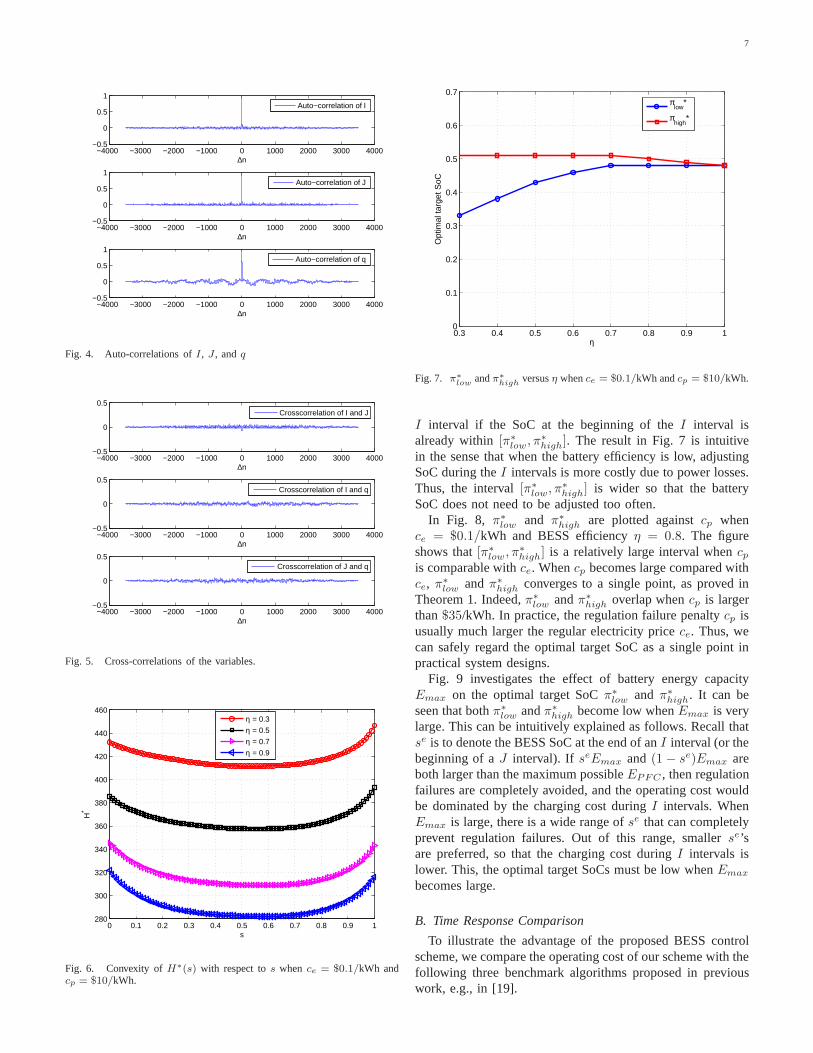
An underlying assumption of our analysis is thatIn, Jnandqn are i.i.d. for differentn, respectively, and that they aremutually independent. To validate this assumption, we plotthe auto-correlations and cross-correlations of the variablesin Figs. 4 and 5, respectively. As we can see from Fig. 4,the auto-correlations of the variables reach the peak when thetime lag is 0 and are close to zero at non-zero time lags,implying that they are approximately independent for differentn. Likewise, Fig. 5 shows that the cross-correlations of thevariables are all close to zero, implying thatI, J , andq aremutually independent.
Before proceeding, let us verify Proposition 1, the convexityof H∗(s) with respect tos, which is a key step in theproof of our main result. Unless otherwise stated, we assumethat Emax = 0.1MWh, Pmax = 1MW, PPFC is uniformlydistributed in[0.5, 1]MW, and the discount factorα = 0.9 inthe rest of the section. In Fig. 6, we plotH∗(s) againsts
0 0.5 1 1.5 2 2.5
x 106
59.9
59.92
59.94
59.96
59.98
60
60.02
60.04
60.06
60.08
60.1
Sample number
Sys
tem
freq
uenc
yFig. 2. System frequency measured at Sacramanto, CA
100
101
102
103
0
0.5
1
x
FI(x
)
100
101
102
103
104
0
0.5
1
x
FJ(x
)
−1 10
0.5
x
Pr{
q=x}
Empirical CDF of I
Empirical CDF of J
Empirical PMF of q
Fig. 3. Empirical distributions ofI, J , andq
whence = $0.1/kWh andcp = $10/kWh. The figure verifiesthat H∗(s) is indeed a convex function ofs, as proved inProposition 1.
A. Optimal Target SoC
In this subsection, we investigate the effect of varioussystem parameters on the optimal target SoCπ∗
low andπ∗high.
The settings of system parameters are the same as that in Fig.6unless otherwise stated. In Fig. 7,π∗
low andπ∗high are plotted
againstη. It can be seen that when the battery efficiencyηis low, [π∗
low, π∗high] is a relatively wide interval. The interval
narrows whenη becomes large, and converges to a single pointwhenη → 1. This is consistent with Theorem 1. Recall thatthere is no need to charge or discharge the battery during an
7
−4000 −3000 −2000 −1000 0 1000 2000 3000 4000−0.5
0
0.5
1
∆n
Auto−correlation of I
−4000 −3000 −2000 −1000 0 1000 2000 3000 4000−0.5
0
0.5
1
∆n
Auto−correlation of J
−4000 −3000 −2000 −1000 0 1000 2000 3000 4000−0.5
0
0.5
1
∆n
Auto−correlation of q
Fig. 4. Auto-correlations ofI, J , andq
−4000 −3000 −2000 −1000 0 1000 2000 3000 4000−0.5
0
0.5
∆n
−4000 −3000 −2000 −1000 0 1000 2000 3000 4000−0.5
0
0.5
∆n
Crosscorrelation of I and q
Crosscorrelation of I and J
−4000 −3000 −2000 −1000 0 1000 2000 3000 4000−0.5
0
0.5
∆n
Crosscorrelation of J and q
Fig. 5. Cross-correlations of the variables.
0 0.1 0.2 0.3 0.4 0.5 0.6 0.7 0.8 0.9 1280
300
320
340
360
380
400
420
440
460
s
H*
η = 0.3
η = 0.5
η = 0.7
η = 0.9
Fig. 6. Convexity ofH∗(s) with respect tos when ce = $0.1/kWh andcp = $10/kWh.
0.3 0.4 0.5 0.6 0.7 0.8 0.9 10
0.1
0.2
0.3
0.4
0.5
0.6
0.7
η
Opt
imal
targ
et S
oC
πlow
*
πhigh
*
Fig. 7. π∗
lowandπ∗
highversusη whence = $0.1/kWh andcp = $10/kWh.
I interval if the SoC at the beginning of theI interval isalready within[π∗
low, π∗high]. The result in Fig. 7 is intuitive
in the sense that when the battery efficiency is low, adjustingSoC during theI intervals is more costly due to power losses.Thus, the interval[π∗
low, π∗high] is wider so that the battery
SoC does not need to be adjusted too often.In Fig. 8, π∗
low and π∗high are plotted againstcp when
ce = $0.1/kWh and BESS efficiencyη = 0.8. The figureshows that[π∗
low , π∗high] is a relatively large interval whencp
is comparable withce. Whencp becomes large compared withce, π∗
low andπ∗high converges to a single point, as proved in
Theorem 1. Indeed,π∗low andπ∗
high overlap whencp is largerthan$35/kWh. In practice, the regulation failure penaltycp isusually much larger the regular electricity pricece. Thus, wecan safely regard the optimal target SoC as a single point inpractical system designs.
Fig. 9 investigates the effect of battery energy capacityEmax on the optimal target SoCπ∗
low and π∗high. It can be
seen that bothπ∗low andπ∗
high become low whenEmax is verylarge. This can be intuitively explained as follows. Recallthatse is to denote the BESS SoC at the end of anI interval (or thebeginning of aJ interval). If seEmax and (1 − se)Emax areboth larger than the maximum possibleEPFC , then regulationfailures are completely avoided, and the operating cost wouldbe dominated by the charging cost duringI intervals. WhenEmax is large, there is a wide range ofse that can completelyprevent regulation failures. Out of this range, smallerse’sare preferred, so that the charging cost duringI intervals islower. This, the optimal target SoCs must be low whenEmax
becomes large.
B. Time Response Comparison
To illustrate the advantage of the proposed BESS controlscheme, we compare the operating cost of our scheme with thefollowing three benchmark algorithms proposed in previouswork, e.g., in [19].

8
0 10 20 30 40 500.1
0.15
0.2
0.25
0.3
0.35
0.4
0.45
0.5
0.55
cp
Opt
imal
targ
et S
oC
πlow
*
πhigh
*
Fig. 8. [π∗
low, π∗
high] vs. cp whence = $0.1/kWh andη=0.8
0.1 0.2 0.3 0.4 0.5 0.6 0.7 0.8 0.9 10.3
0.35
0.4
0.45
0.5
0.55
0.6
Emax
(MWh)
Opt
imal
targ
et S
oC
π
low*
πhigh
*
Fig. 9. [π∗
low, π∗
high] vs.Emax whence = $0.1/kWh andcp = $10/kWh.
• No additional charging duringI intervals. Referred to“No recharging” in the figures.
• Recharge up to100% during I intervals. Referred to as“Aggressive recharging” in the figures.
• Recharge with upper and lower target SoCs. This schemeis similar to our proposed scheme, except that the targetSoCs are set heuristically (instead of optimized in ouralgorithm). In upper and lower target SoCs are set tobe 0.92 and 0.73, respectively in [19]. This scheme isreferred to as “Heuristic recharging” in the figures.
In particular, we run a time-response simulation using the real-time frequency measurement data in Fig. 2. The probabilityof encountering regulation failures is plotted in Fig. 10. More-over, the time-aggregate operating costs (without discounting)are plotted in Figs. 11 and 12 whenEmax = 0.1MWh andEmax = 1.5MWh, respectively. It can be seen from Figs. 11and 12 that both ”No recharging” and ”Aggressive recharging”algorithms yield much higher cost than the optimal algorithmproposed in the paper. This is because the battery SoC is
0 0.5 1 1.5
10−1
Emax
(MWh)
Pro
babi
lity
of r
egul
atio
n fa
ilure
Optimal algorithmNo rechargingAggressive rechargingHeuristic recharging
Fig. 10. Comparison of regulation failure probability whence = $0.1/kWh,cp = $10/kWh andη=0.8
0 10 20 30 40 50 60 70 80−0.5
0
0.5
1
1.5
2
2.5
3x 10
5
Time (hour)
Cos
t ($)
Optimal algorithmNo rechargingAggressive rechargingHeuristic recharging
Fig. 11. Comparison of time-aggregate costs whenEmax = 0.1MWh,ce = $0.1/kWh, cp = $10/kWh andη=0.8
often too low (with ”No recharging”) or too high (with ”Ag-gressive charging”), yielding much higher regulation failureprobabilities, as shown in Fig. 10. On the other hand, withoptimal target SoC, the proposed algorithm reduces both theoperating cost and regulation failure probability compared with”Heuristic recharging”.
C. Optimal BESS Planning
In Fig. 13, we verify Theorem 2 and investigate the effectof BESS energy capacityEmax on the operating costH∗.Here, ce = $0.1/kWh, cp = $10/kWh, η = 0.8, andEmax
varies from 0.05MWh to to 10MWh. It can be see thatH∗(s)is a decreasing convex function ofEmax for all initial SoCs. This implies that there exists an optimal BESS energycapacity Emax that hits the optimal balance between thecapital investment and operating cost.

9
0 10 20 30 40 50 60 70 80−2
0
2
4
6
8
10
12x 10
4
Time (hour)
Cos
t ($)
Optimal algorithmNo rechargingAggressive rechargingHeuristic recharging
Fig. 12. Comparison of time-aggregate costs whenEmax = 1.5MWh,ce = $0.1/kWh, cp = $10/kWh andη=0.8
0.1 0.2 0.3 0.4 0.5 0.6 0.7 0.8 0.9 10
100
200
300
400
500
600
700
800
900
1000
Emax
(MWh)
H*
H*(0.1)H*(0.3)H*(0.5)H*(0.7)H*(0.9)
Fig. 13. H∗(s) vs. Emax when ce = $0.1/kWh, cp = $10/kWh, andη = 0.8.
VII. C ONCLUSIONS
We studied the optimal planning and control for BESSsparticipating in the PFC regulation market. We show that theoptimal BESS control is to charge or discharge the BESSduring I intervals until its SoC reaches a target value. Wehave proved that the optimal target SoC is a range that isinvariant with respect to the BESS SoCs at the beginning oftheI intervals. This implies that the optimal target SoC can becalculated offline and remain unchanged over the entire systemtime. Hence, the operation complexity can be kept very low.Moreover, the target SoC range reduces to a point in practicalsystems, where the penalty rate for regulation failure is muchlarger than the regular electricity price. It was also shownthatthe optimal operating cost is a decreasing convex functionof the BESS energy capacity, implying the existence of anoptimal energy capacity that balances the capital investmentof BESS and the operating cost.
Other than PFC, BESSs can serve multiple purposes, such asdemand response, energy arbitrage, and peak shaving. Differ-
ent services require different energy and power capacities. Forexample, PFC reserves do not require high energy capacity,but are sensitive to regulation failures. On the other hand,high energy capacity is needed for demand response, energyarbitrage, and peak shaving. It is an interesting future researchtopic to study the optimal combining of these services in asingle BESS.
APPENDIX APROOF OFPROPOSITION1
Proof: First, calculate
∂H∗(s)
∂s=
∂h(s, π∗)
∂s(27)
+ αp1
∫ Q∗
1
0
∫ Q∗
2
0
∂H∗(Q∗3)
∂sfEPFC
(e)fI(i)dedi
+ αp−1
∫ Q∗
1
0
∫ Q∗
4
0
∂H∗(Q∗5)
∂sfEPFC
(e)fI(i)dedi
where
Q∗2 =
(1 − s)Emax − sgn(π∗ − s)Pmaxi
η, (28)
Q∗3 =
sEmax + sgn(π∗ − s)Pmaxi+ ηe
Emax
, (29)
Q∗4 = η(sEmax + sgn(π∗ − s)Pmaxi), (30)
Q∗5 =
sEmax + sgn(π∗ − s)Pmaxi − e/η
Emax
, (31)
andQ∗1 is the same asQ1 in (13) except thatπ is replaced by
π∗ in the definition. After some manipulations, we have
H∗(2)(s) = a(s) (32)
+ αp1
∫ Q∗
1
0
∫ Q∗
2
0
H∗(2) (s′)∣
∣
s′=Q∗
3fEPFC
(e)fI(i)dedi
+ αp−1
∫ Q∗
1
0
∫ Q∗
4
0
H∗(2) (s′)∣
∣
s′=Q∗
5
fEPFC(e)fI(i)dedi,
whereH∗(2)(s) := ∂2H∗(s)∂s2
and
a(s) =−sgn(π∗ − s)Emax
Pmax
(
r(s, π∗)Emax + u(π∗))
fI (Q∗1)
+
∫ Q∗
1
0
∂2costp (s′)
∂s′2
∣
∣
∣
∣
s′=s+PmaxiEmax
fI(i)di. (33)
We claim thata(s) is non-negative for alls. To see this, notethat
−sgn(π∗ − s)(
r(s, π∗)Emax + u(π∗))
≥ 0
for all s due to the necessary condition of optimalπ∗ in(24) and (25). Thus, the first term ofa(s) is non-negative.Moreover, the integrand in the second term ofa(s) is alwaysnon-negative as:
∂2costp(s)
∂s2
= cpE2max
(
p1η2
fEPFC(Emax(1− s)) + p−1η
2fEPFC(Emaxs)
)
≥ 0,(34)

10
where the equality is obtained by taking the second-orderderivative of (15) overse at se = s, and the inequality isdue to the fact that PDF functions are non-negative. Thus,a(s) ≥ 0.
Define two operatorsD andT such that
Df(s) = αp1
∫ Q∗
1
0
∫ Q∗
2
0
f (s′)∣
∣
s′=Q∗
3fEPFC
(e)fI(i)dedi
+ αp−1
∫ Q∗
1
0
∫ Q∗
4
0
f (s′)∣
∣
s′=Q∗
5fEPFC
(e)fI(i)dedi,
andTf(s) = a(s) +Df(s). (35)
It will be shown in Lemma 2 that the operatorT is acontraction mapping. Thus,H∗(2)(s) is the fixed point ofequationf(s) = Tf(s), and the fixed point can be achievedby iteration
f (k+1)(s) = Tf (k)(s).
Letting f (0)(s) = 0 for all s, we can calculate the fixed pointas
H∗(2)(s) =
∞∑
i=0
Ki(s),
whereK0(s) = a(s) andKi(s) = DKi−1(s). Note thatD isa summation of two integrals, and therefore is non-negativewhen the integrand is non-negative. Thus, allKi(s) ≥ 0,becauseK0(s) = a(s) ≥ 0. As a result,H∗(2)(s) ≥ 0 forall s. This completes the proof.
Lemma2. The operatorT defined in (35) is a contractionmapping.
To prove the lemma, we can show thatT satisfies followingBlackwell Sufficient Conditions for contraction mapping.
• (Monotonicity) For any pairs of functionsf(s) andg(s)such thatf(s) ≤ g(s) for all s, Tf(s) ≤ Tg(s).
• (Discounting)∃β ∈ (0, 1) : T (f + b)(s) < Tf(s) +βb ∀f, b ≥ 0, s.
Proof: Obviously,Df(s) ≤ Dg(s) for any pairs of func-tionsf(s) ≤ g(s), because the operators is a summation of twointegrals with non-negative integrands. Thus,Tf(s) ≤ Tg(s),and the Monotonicity condition holds.
To prove the discounting property, notice that
T (f + b)(s) = a(s) +D(f + b)(s) = a(s) +Df(s) +Db
= Tf(s) +Db, (36)
because integrals are linear operations. Moreover,
Db = αb
(
p1
∫ Q∗
1
0
∫ Q∗
2
0
fEPFC(e)fI(i)dedi
+p−1
∫ Q∗
1
0
∫ Q∗
4
0
fEPFC(e)fI(i)dedi
)
≤ αb
(
p1
∫ Q∗
1
0
fI(i)di+ p−1
∫ Q∗
1
0
fI(i)di
)
≤ αb(p1 + p−1)
= αb. (37)
Here, the inequalities are due to the fact that the integralsofPDF functions are no larger than 1. Sinceα is a discountingfactor that is smaller than 1, the Discounting condition holds.
APPENDIX BPROOF OFLEMMA 1
Proof:
∂u(π)
∂π
= αp1
∫
(1−π)Emaxη
0
H∗(2) (s)∣
∣
s=π+ ηeEmax
fEPFC(e)de
+αp−1
∫ ηπEmax
0
H∗(2) (s)∣
∣
s=π− eηEmax
fEPFC(e)de
≥ 0, (38)
where the equality is obtained by differentiating (23) overπ, and the inequality is due to the fact thatH∗(2) (s) ≥ 0for all s, as proved in Proposition 1. Thus,u(π) increaseswith π. Meanwhile, bothr1(π) and r2(π) are increasingfunctions ofπ, becauseFEPFC
(x) is a decreasing function ofx. Hence, bothr1(π)Emax+u(π) andr2(π)Emax+u(π) areincreasing functions ofπ. Moreover, whenπ increases froms− to s+, r(s, π)Emax + u(π) increases by
(
1η− η)
ce from
r2(s−)Emax+u(s−) to r1(s
+)Emax+u(s+). This completesthe proof.
APPENDIX CPROOF OFTHEOREM 2
Proof: The proof of convexity ofH∗(s) with respect toEmax is similar to that for Proposition 1, and thus is shortenedhere. We first calculate
∂2H∗(s)
∂E2max
=a(s, Emax)
+ αp1
∫ Q∗
1
0
∫ Q∗
2
0
∂2H(s′)
∂E2max
∣
∣
∣
∣
s′=Q∗
3
fEPFC(e)fI(i)dedi
+ αp1FI(Q∗1)
∫
(1−π∗)Emaxη
0
∂2H(s′)
∂E2max
∣
∣
∣
∣
s′=π∗Emax+ηeEmax
fEPFC(e)de
+ αp−1
∫ Q∗
1
0
∫ Q∗
4
0
∂2H(s′)
∂E2max
∣
∣
∣
∣
s′=Q∗
5
fEPFC(e)fI(i)dedi
+ αp−1FI(Q∗1)
∫ ηπ∗Emax
0
∂2H(s′)
∂E2max
∣
∣
∣
∣
s′=π∗− eηEmax
fEPFC(e)de,
(39)where
a(s, Emax)
=−sgn(π∗ − s)|π∗ − s|2
PmaxEmax
fI(Q∗1) (r(s, π
∗)Emax + u(π∗))
+ cpp1
(
1− π∗
η
)2
fEPFC
(
(1− π∗)Emax
η
)
FI(Q∗1)
+ cpp−1(ηπ∗)2fEPFC
(ηπ∗Emax) FI(Q∗1)
+
∫ Q∗
1
0
cp
(
p1
(
1− s
η
)2
fEPFC(Q∗
2) + p−1(ηs)2fEPFC
(Q∗4)
)
fI(i)di.
(40)

11
We claim thata(s, Emax) ≥ 0 for all s and Emax. To seethis, note that the first term is always non-negative, because
−sgn(π∗ − s) (r(s, π∗)Emax + u(π∗)) ≥ 0
due to (24) and (25). Moreover, the remaining terms are non-negative due to the non-negativeness of PDFs and CCDFs.
Same as the proof in Proposition 1, we can show that theright hand side of (39) is a contraction mapping. Thus, we cancalculate∂2H∗(s)
∂E2max
as a fixed point and get
∂2H∗(s)
∂E2max
=
∞∑
i=0
Ki(s, Emax),
where all Ki(s, Emax) ≥ 0. This implies that∂2H∗(s)∂E2
max≥ 0,
and thusH∗(s) is convex with respect toEmax.Now we proceed to prove thatH∗(s) is a decreasing
function of Emax. We first show that the optimal single-stage costh∗(s) = minπ h(s, π) decreases withEmax. Then,the decreasing monotonicity ofH∗(s) with respect toEmax
can be proved by the monotonicity property of contractionmapping, which is stated in Lemma 2.
Recall that∂h(s,π)∂π
= r(s, π)EmaxFI(Q1), wherer(s, π) isdefined in (22). Thus, the optimalπ that minimizesh(s, π)satisfies
r(s, π) = 0. (41)
Furthermore, we can calculate that
∂h(s, π)
∂Emax
=
(
1π≥s
1
η− 1π<sη
)
ce|π − s|FI (Q1)
− cpp1(1 − π)
ηFEPFC
(
Emax(1 − π)
η
)
FI (Q1)
− cpp−1ηπFEPFC(ηEmaxπ) FI (Q1) (42)
Substituting (41) to (42), we have
∂h∗(s)
∂Emax
= −
(
1π1st≥s
1
η+ 1π1st<sη
)
cesFI (Q1)
−cpp1η
FEPFC
(
Emax(1− π1st)
η
)
FI (Q1)
≤ 0, (43)
whereπ1st is the minimizer ofh(s, π). (43) implies thath∗(s)decreases withEmax for all s.
Next, note that the Bellman equation of infinite-horizondynamic programming is a contraction mapping [17]. Let
TH(s) = minπ∈[0,1]
h(s, π)+αEI,EPFC ,q [H(g(s, π, I, EPFC , q))]
(44)be the contraction operator corresponding to the Bellmanequation in (10). Then,
H∗(s) = limk→∞
(T kH0)(s)
for all s.Starting withH0(s) = 0, we have
H1(s) = TH0(s) = h∗(s).
Let h∗+(s) (or H+k (s)) andh∗−(s) (or H−
k (s)) denoteh∗(s)(or Hk(s)) with BESS energy capacityE+
max and E−max,
respectively. We have proved thath∗+(s) ≤ h∗−(s), orequivalentlyH+
1 (s) ≤ H−1 (s), if E+
max ≥ E−max. Due to the
monotonicity property of contraction mapping,
H+k (s) ≤ H−
k (s)
as long asH+k−1(s) ≤ H−
k−1(s) for all k. Takingk to infinity,we haveH∗+(s) ≤ H∗−(s) when E+
max ≥ E−max. This
completes the proof.
APPENDIX DALGORITHM TO OBTAIN π∗
low AND π∗high
The traditional algorithms to solve infinite-horizon dynamicprogramming problems, e.g., value iteration and policy itera-tion algorithms, involve iterative steps, where in each iteration,the policy π(i) is updated for each system state (i.e., BESSSoC)i. In our problem, the state space is continuous in[0, 1].If it is discretized intoN levels, i.e.,i ∈ {0, δ, 2δ, · · · , 1}whereδ = 1
N−1 , thenN optimization problems, one for eachπ(i), need to be solved in each iteration.
Based on the state-invariant property ofπ∗low andπ∗
high, thecomplexity of solving the dynamic programming problem canbe greatly reduced. Definepij(π) = Pr{sn+1 = j|sn = i, π},which can be calculated from the distributions ofI, J , q, andEPFC . For any given pair ofd = (πlow , πhigh), we have
pdij.= pij(π(i)) =
pij(πlow) i < πlow
pij(πhigh) i > πlow
pij(i) πlow ≤ i ≤ πhigh
(45)
Let Pd be the matrix ofpdij , andHd be the vector ofHd(i).Likewise, define vectorhd, whoseith entry ish(i, πlow) wheni < πlow, h(i, πhigh) wheni > πhigh, andh(i, i) whenπlow ≤i ≤ πhigh. Then,Hd can be obtained as the solution of
(
I− αPd)
Hd = h
d. (46)
The optimalπ∗low andπ∗
high can then be obtained by solving
minπlow,πhigh
βT(
I− αPd)−1
hd, (47)
whereβ is an arbitrary vector3. In contrast to the traditionalvalue iteration and policy iteration approaches, no iteration isrequired here.π∗
low andπ∗high can be obtained by solving one
optimization problem (47) with two scalar variables only.
REFERENCES
[1] P. Kundur,Power System Stability and Control. McGraw-Hill, 1994.[2] F. C. Schweppe, R. D. Tabors, J. L. Kirtley, H. R. Outhred,F. H.
Pickel, and A. J. Cox, “Homeostatic utility control,”IEEE Trans. PowerApparatus and Systems, vol. PAS-99, no. 3, pp. 1151–1163, 1980.
[3] C. Zhao, U. Topcu, N. Li, and S. Low, “Design and stabilityof load-sideprimary frequency control in power systems,”IEEE Trans. AutomaticControl, vol. 59, no. 5, pp. 1177–1189, 2014.
[4] C. Zhao, U. Topcu, and S. H. Low, “Optimal load control viafrequencymeasurement and neighborhood area communication,”IEEE Trans.Power Systems, vol. 28, no. 4, pp. 3576–3587, 2013.
3The fact thatπ∗
lowandπ∗
highminimize H(i) for all i implies that the
optimal solution to (47) is the same for allβ.

12
[5] J. Short, D. G. Infield, L. L. Freriset al., “Stabilization of grid frequencythrough dynamic demand control,”IEEE Trans on Power Systems,vol. 22, no. 3, pp. 1284–1293, 2007.
[6] A. Molina-Garcia, F. Bouffard, and D. S. Kirschen, “Decentralizeddemand-side contribution to primary frequency control,”IEEE Trans.Power Systems, vol. 26, no. 1, pp. 411–419, 2011.
[7] S.-J. Lee, J.-H. Kim, C.-H. Kim, S.-K. Kim, E.-S. Kim, D.-U. Kim,K. K. Mehmood, and S. U. Khan, “Coordinated control algorithm fordistributed battery energy storage systems for mitigatingvoltage andfrequency deviations,”To appear, IEEE Trans. Smart Grid.
[8] B. Xu, A. Oudalov, J. Poland, A. Ulbig, and G. Andersson, “BESScontrol strategies for participating in grid frequency regulation,” in WorldCongress, vol. 19, no. 1, 2014, pp. 4024–4029.
[9] A. Oudalov, D. Chartouni, C. Ohler, and G. Linhofer, “Value analysisof battery energy storage applications in power systems,” in IEEE PESPower Systems Conference and Exposition, 2006, pp. 2206–2211.
[10] P. Denholm, E. Ela, B. Kirby, and M. Milligan, “The role of energy stor-age with renewable electricity generation,”Technical Report, NationalRenewable Energy Laborabory, 2010.
[11] D. Kottick, M. Blau, and D. Edelstein, “Battery energy storage forfrequency regulation in an island power system,”IEEE Trans. EnergyConversion, vol. 8, no. 3, pp. 455–459, 1993.
[12] T. Borsche, A. Ulbig, M. Koller, and G. Andersson, “Power and energycapacity requirements of storages providing frequency control reserves,”in IEEE Power and Energy Society General Meeting (PES), 2013, pp.1–5.
[13] P. Mercier, R. Cherkaoui, and A. Oudalov, “Optimizing abattery energystorage system for frequency control application in an isolated powersystem,”IEEE Trans. on Power Systems, vol. 24, no. 3, pp. 1469–1477,2009.
[14] M. R. Aghamohammadi and H. Abdolahinia, “A new approachforoptimal sizing of battery energy storage system for primaryfrequencycontrol of islanded microgrid,”Int. J. Electrical Power and EnergySystems, vol. 54, pp. 325–333, 2014.
[15] K. Spees and L. B. Lave, “Demand response and electricity marketefficiency,” Electricity J., vol. 20, no. 3, pp. 69–85, 2007.
[16] S. Isser, “FERC order 719 and demand response in ISO markets,” GoodCompany Associates/ERCOT Technical Report, 2009.
[17] D. P. Bertsekas,Dynamic programming and optimal control. AthenaScientific Belmont, MA, 1995, vol. 1 and 2, no. 2.
[18] Y. Liu, L. Zhan, Y. Zhang, P. Markham, D. Zhou, J. Guo, Y. Lei,G. Kou, W. Yao, J. Chai, and Y. Liu, “Wide-area measurement systemdevelopment at the distribution level: an fnet/grideye example,” IEEETransactions on Power Delivery, vol. PP, no. 99, pp. 1–1, 2015.
[19] A. Oudalov, D. Chartouni, and C. Ohler, “Optimizing a battery energystorage system for primary frequency control,”IEEE Trans. PowerSystems, vol. 22, no. 3, pp. 1259–1266, 2007.