protection coordination in networks with renewable energy

1

Protection Coordination in Networks with

Renewable Energy Sources

A thesis submitted to The University of Manchester for the degree of

Master of Philosophy (MPhil)

in the Faculty of Engineering and Physical Sciences

2014

Zhiqi Han

School of Electrical and Electronic Engineering

2

Table of Contents

TABLE OF CONTENTS...................................................................................................... 2

LIST OF FIGURES AND TABLES .................................................................................... 5

LIST OF ABBREVIATIONS .............................................................................................. 7

ABSTRACT .......................................................................................................................... 8

DECLARATION................................................................................................................... 9

INTELLECTUAL PROPERTY ........................................................................................... 9

ACKNOWLEDGEMENTS ................................................................................................ 10

1.INTRODUCTION............................................................................................................ 11

2.PROTECTION SYSTEM ................................................................................................ 13

2.1 Chapter introduction ..................................................................................................... 13

2.2 Basic elements of a protection system ......................................................................... 13

2.3 Overcurrent protection .................................................................................................. 14

2.3.1 Overcurrent relaying .............................................................................................. 14

2.3.2 Fuses ....................................................................................................................... 16

2.3.3 Directional relays ................................................................................................... 17

2.3.4 Current and voltage transformer ........................................................................... 18

2.3.5 Equipment damage curves .................................................................................... 19

2.3.6 Transformer inrush current.................................................................................... 19

2.4 Distance protection ....................................................................................................... 20

2.4.1 Distance relay ......................................................................................................... 20

2.4.2 Types of distance relays ........................................................................................ 20

2.4.3 The effect of arc resistance on distance protection .............................................. 21

2.5 Chapter summary .......................................................................................................... 22

3.PROTECTION COORDINATION ................................................................................ 23


3.2 Overcurrent protection coordination in different network configurations ................ 23

3.2.1 Basic overcurrent protection coordination rules .................................................. 23

3.2.2 Overcurrent protection coordination in radial network ....................................... 24

3.2.3 Protection coordination in networks with multiple sources ................................ 26

3.2.4 Protection coordination in meshed networks ....................................................... 27

3.3 Distance protection coordination ................................................................................. 28

3.3.1 Protection coordination between distance relays ................................................. 29

3.3.2 Protection coordination between distance and overcurrent relays...................... 29

3

3.4 Chapter summary .......................................................................................................... 31

4.IMPACTS OF RENEWABLE ENERGY SOURCES ON PROTECTION

COORDINATION .............................................................................................................. 32


4.2 False tripping of overcurrent relays ............................................................................. 32

4.3 Loss of protective devices grading............................................................................... 33

4.4 Blinding of overcurrent relays...................................................................................... 33

4.5 The effect of infeed on the distance protection ........................................................... 35

4.6 Chapter summary .......................................................................................................... 37

5.COMPUTER SIMULATION FAULTED DISTRIBUTION NETWORKS USING

DIGSILENT ........................................................................................................................ 38


5.2 Network modeling......................................................................................................... 38

5.3 Protection coordination in a MV network prior to the DGs connection.................... 40

5.3.1 Selecting protective devices .................................................................................. 40

5.3.2 Pick-up currents of relays and fuses ..................................................................... 41

5.3.3 Explanation of the protection coordination .......................................................... 41

5.3.4 Equipment damage curves and inrush current ..................................................... 43

5.3.5 Relay parameters .................................................................................................... 44

5.3.6 Assessment of different fault cases....................................................................... 45

5.4 Protection coordination in a MV network with DG connected .................................. 47

5.4.1 Loss of grading....................................................................................................... 49

5.4.2 False tripping .......................................................................................................... 51

5.4.3 Blinding .................................................................................................................. 53

5.5 Assessment of different fault cases .............................................................................. 55

5.6 Chapter summary .......................................................................................................... 57

6.MESHED NETWORKS SIMULATED IN DIGSILENT ............................................ 65


6.2 Network modeling......................................................................................................... 65

6.3 Meshed network without DGs...................................................................................... 66

6.3.1 The selection and settings of protective devices .................................................. 66


6.3.3 Relay parameters and characteristics .................................................................... 71


6.4 Meshed network with DGs connected ......................................................................... 73

4

6.4.1 The network modeling and the protection system ............................................... 73



6.5 Chapter summary .......................................................................................................... 78

7.CONCLUSION ................................................................................................................ 79

7.1 Project summary............................................................................................................ 79

7.2 Future work ................................................................................................................... 81

8.REFERENCES ................................................................................................................. 82

9.APPENDICES .................................................................................................................. 85

Appendix 1: DIgSILENT PowerFactory ........................................................................... 85

A.1.1 Introduction ........................................................................................................... 85

A.1.2 Short-Circuit Analysis .......................................................................................... 85

A.1.2 Protection Analysis ............................................................................................... 86

A.1.3 Time-overcurrent plot ........................................................................................... 87

A.1.4 Time-Distance diagram ........................................................................................ 88

Appendix 2 Relay characteristics in the time-overcurrent plot ........................................ 89

A.2.1 Without DGs connected........................................................................................ 89

A.2.2 With DGs connected ............................................................................................. 89

Appendix 3 Network data for meshed distribution network data .................................... 92

A.2.1 Induction generator parameters ............................................................................ 92

A.2.2 Line data ................................................................................................................ 92

A.2.3 Transformer data and load data ............................................................................ 93

Appendix 4 Relay parameters for the meshed network .................................................... 94

Word count: 18198

5

List of Figures and Tables

Figure 2-1 Single-line connection of protective relay ...................................................... 14

Figure 2-2 Different characteristics of OC relays ............................................................. 15

Figure 2-3 A time overcurrent plot of for the fuses .......................................................... 17

Figure 2-5 Example of a cable damage curve ................................................................... 19

Figure 2-6 Distance relay characteristics on the R-X diagram......................................... 21

Figure 2-7 The effect of arc resistance on the MHO relay ............................................... 22

Figure 3-1 The coordination of IDMT relays .................................................................... 25

Figure 3-2 Coordination in a multiple sources system ..................................................... 26

Figure 3-3 A meshed network with multiple sources ....................................................... 27

Figure 3-4 Coordination between directional IDMT relays around clockwise ............... 28

Figure 3-5 Coordination between distance relays ............................................................. 30

Figure 3-6 Coordination between distance and OC relays ............................................... 30

Figure 4-1An illustration of a situation where false tripping may occur ......................... 33

Figure 4-2 An example of blinding .................................................................................... 34

Figure 4-3 An example solution for the blinding problem ............................................... 35

Figure 5-1 Singe line diagram of the distribution network without DGs ........................ 39

Figure 5-2 Singe line diagram of the large wind farm ...................................................... 39

Figure 5-3 Singe line diagram of the small wind farm ..................................................... 39

Figure 5-4 Moving characteristic showing the grading margin ....................................... 42

Figure 5-5 The phase element of relay characteristics in the time overcurrent plot ....... 42

Figure 5-6 Example of transformer damage curve and inrush current ............................ 43

Figure 5-7 Relay parameters with the DG connected ....................................................... 45

Figure 5-8 Single phase fault .............................................................................................. 46

Figure 5-9 Three phase fault ............................................................................................... 46

Figure 5-10 Two phase fault ............................................................................................... 46

Figure 5-11 Overall diagram of the protection system after DG integration .................. 48

Figure 5-12 Flow chart on the coordination process after DG connection ...................... 49

Figure 5-13 Examples of three phase faults with or without DGs being connected ....... 51

Figure 5-14 False tripping (a) Fuse (b) directional relay .................................................. 52

Figure 5-15 Example of a 3-phase fault for blinding ........................................................ 52

Figure 5-16 A 3-phase fault located at Bus 6 showing in ................................................. 54

Figure 5-17 Three-phase fault at small wind farm, showing ............................................ 56

Figure 5-18 Single phase fault at the large wind farm ...................................................... 57

6

Figure 5-19 Relay parameters for the main network ........................................................ 60

Figure 5-20 Relay parameters for the large wind farm ..................................................... 62

Figure 5-21 Relay parameters for the small wind farm .................................................... 63

Figure 6-1 Singe line diagram of the meshed distribution network ................................. 66

Figure 6-2 The R-X plots display a 2-phase fault ............................................................. 67

Figure 6-3 Example for overlapping of distance relays .................................................... 69

Figure 6-4 Time-distance plot displays the distance relay working as a back-up ........... 70

Figure 6-5 Time-distance plot that displays the OC relay working as a back-up ........... 70

Figure 6-6 The parameters of relay 3a ............................................................................... 71

Figure 6-7 Characteristics of distance relays in clockwise direction ............................... 72

Figure 6-8 Three phase fault at 90% of cable 3................................................................. 73

Figure 6-9 Singe line diagram of the meshed distribution network with DGs ................ 74

Figure 6-10 Example for under reaching of a distance relay............................................ 75

Figure 6-11 The time distance plot displays the relays in the clockwise direction ......... 76

Figure 6-12 Two phase fault at cable 2 .............................................................................. 77

Figure 6-13 Three phase fault at cable 4 ............................................................................ 78

Figure 9-1 Short circuit with the 'Complete' method ........................................................ 86

Figure 9-2 Relay model dialogue with selected type ........................................................ 87

Figure 9-3 Short circuit sweep method .............................................................................. 88

Figure 9-4 Relay characteristic curves for earth elements ................................................ 89

Figure 9-5 Relay characteristic curves for phase elements in the main network ............ 89

Figure 9-6 Relay characteristic curves for earth elements in the main network ............. 90

Figure 9-7 Relay characteristic curves for phase elements in the large wind farm ........ 91

Figure 9-8 Relay characteristic curves for earth elements in the large wind farm .......... 91

Figure 9-9 Relay characteristic curves for phase elements in the small wind farm ........ 91

Figure 9-10 Relay characteristic curves for earth elements in the small wind farm ....... 92

Figure 9-11 Relay parameters without DGs ...................................................................... 96

Figure 9-12 Relay parameters with DGs ......................................................................... 100

Table 2-1 Relay characteristics according IEC 60255 ...................................................... 16

Table 5-1 Fuse data ............................................................................................................. 41

Table 9-1 Induction generator parameters ......................................................................... 92

Table 9-2 Transformer data ................................................................................................ 93

Table 9-3 Load data............................................................................................................. 93

7

List of Abbreviations

DG Distributed Generator

OC Overcurrent

CB Circuit Breaker

CT Current Transformer

VT Voltage Transformer

IDMT Inverse Definite Minimum Time

SI Standard Inverse,

VI Very Inverse

EI Extremely Inverse

MMT Minimum Melt Time

TCT Total Clearing Time

TMS Time Multiplier Setting

CTI Coordination Time Interval

8

Abstract

The increased distributed generators (DGs) in distribution networks are causing

protection coordination problems. Due to the many generation sources supplying the

distribution network, the conventional protective devices have become insufficient to

ensure the proper protection coordination in case of a fault.

This dissertation illustrates the summary of the DGs’ influences and an overview of the

approaches for selecting and coordinating the protection system with or without DGs.

Two example networks have been used to demonstrate the specific coordinating

methods and problems for an overcurrent-based scheme and a distance-based scheme

with the help of the DIgSILENT PowerFactory software package. One example is a

radial medium voltage network mainly protected by overcurrent (OC) relays, which has

potential false tripping and blinding effects. Another one is a typical UK meshed

distribution network which may suffer the under reaching for distance relays that occurs

on the basis of the distance-based protection scheme. The protection system for each

network will be used to prove the success of the derived settings and also the successful

coordination of protective devices by discussing the time-overcurrent plot, R-X plot and

time-distance plot. The proposed new protection schemes for these distribution

networks have achieved the orderly protection operation in case of a fault, namely the

appropriate protection coordination.

9

Declaration

No portion of the work referred to in this dissertation has been submitted in support of

an application for another degree or qualification of this or any other university or

institute of learning.

Intellectual Property

i) The author of this dissertation (including any appendices and/or schedules to this

dissertation) owns certain copyright or related rights in it (the “Copyright”) and he has

given The University of Manchester certain rights to use such Copyright, including for

administrative purposes.

ii) Copies of this dissertation, either in full or in extracts and whether in hard or

electronic copy, may be made only in accordance with the Copyright, Designs and

Patents Act 1988

(as amended) and regulations issued under it or, where appropriate, in accordance with

licensing agreements which the University has from time to time. This page must form

part of any such copies made.

iii) The ownership of certain Copyright, patents, designs, trademarks and other

intellectual property (the “Intellectual Property”) and any reproductions of copyright

works in the dissertation, for example graphs and tables (“Reproductions”), which may

be described in this dissertation, may not be owned by the author and may be owned by

third parties. Such Intellectual Property and Reproductions cannot and must not be

made available for use without the prior written permission of the owner(s) of the

relevant Intellectual Property and/or Reproductions.

iv) Further information on the conditions under which disclosure, publication and

commercialisation of this dissertation, the Copyright and any Intellectual Property

and/or Reproductions described in it may take place is available in the University IP

Policy (see http://documents.manchester.ac.uk/display.aspx?DocID=487), in any

relevant Dissertation restriction declarations deposited in the University Library, The

University Library’s regulations (see

http://www.manchester.ac.uk/library/aboutus/regulations) and in The University’s

Guidance for the Presentation of Dissertations.

http://documents.manchester.ac.uk/display.aspx?DocID=487

http://www.manchester.ac.uk/library/aboutus/regulations

10

Acknowledgements

I would like to express my gratitude to my supervisor, Professor Vladimir Terzija, who

has given me the chance to pursue this degree and perform this research work under his

guidance. His great help has supported me not only in terms of academic knowledge but

also in my life abroad. I would also like to thank Mr. Georgios Peltekis, who has given

me valuable materials for my dissertation and support when I required.

Finally, for their encouragement and support I would like to thank my parents. They

have given me so much comfort and care during the past year.

11

1. Introduction

Historically, electric power systems were designed as a pure radial networks, which

have gradually evolved into meshed networks. Radial operations have been applied for

years in order to protect medium voltage distribution networks and their greatest benefit

is their simplicity. However, with a much greater focus on the improvement in power

quality, system reliability and environmental problems, meshed networks and the

penetration of distributed generators are becoming the preferred options.

Despite the positive aspects of the meshed configuration and DG connection, there are

also some difficulties such as protection coordination problems once they have been

applied. One of the most significant concerns is the coordination between protective

devices. As the conventional distribution network is radial in nature, the primary

substation is the only power source to supply the downstream load and to sustain the

fault current (an example of a radial network can be found in Section 5.3, the

distribution network with DGs connected can be found in Section 5.4). Distributed

resources in a meshed structure invalidate the natural radial configuration of the

distributed network (Section 6.2). Obviously, the presence of DG would have an impact

on the fault current level. Moreover, the conventional network is fed by a utility active

resource while the system with the DGs connection is supplied by more than one active

resource. This causes a change in the fault currents’ directions. In this dissertation, the

feeder protection issues that result from DG propagation are considered. Sensitivity and

selectivity are the typical feeder protection requirements. The relay operation can be

delayed or, even worse, totally blocked because of the blinding operation (Explained in

Section 4.4), which will then have an impact on sensitivity. In addition, unnecessary

tripping occurs at the adjacent feeder that the DG is connected to. This can adversely

affect selectivity. These effects become a problem when considering the protection

coordination, which is decided by the DG capacity, the DG location and the number of

DGs connected to the system. Moreover, the complexity of the network topology makes

the calculation process extremely difficult.

This dissertation firstly gives a brief introduction to power system protection in Chapter

2, which includes the basic elements of an overcurrent protection system and a distance

protection system. Then Chapter 3 shows an analysis of coordination problems, and

12

then discusses the various protection schemes in a conventional radial network with a

single source, a distribution network with DG connections and a mesh network with or

without DGs. The protection coordination problem is discussed in detail in these

protection schemes, which include the coordination of fuses, overcurrent relays and

distance relays. The effects caused by the proliferation of DGs are given in Chapter 4.

There are 4 major influences: loss of coordination grading, false tripping, blinding, and

under reaching. Each effect is explained and solutions are proposed. Chapter 5 and

Chapter 6 illustrate the protection system in examples of distribution networks in detail.

The protection systems for each network are simulated in DIgSILENT software, which

includes the network modeling, the coordination procedures, the analysis of the time

overcurrent plot, and the setting of relay parameters. The project summary and future

work are discussed in Chapter 7.

13

2. Protection system

2.1 Chapter introduction

This chapter gives a brief explanation about protection systems in terms of overcurrent

protection and distance protection, including the description of different types of

protective devices that will be used in this project.

2.2 Basic elements of a protection system

The protection arrangement for any power system must take into account the following

basic principles: reliability (including dependability and safety), speed and selectivity.

The reduction in the number and duration of the interruptions to the electricity users can

enhance the reliability of the power supply. Power quality can also be improved with a

faster pick up time to minimize the likelihood of voltage sags, voltage flicker etc.

The protective relay is the most frequently used protection device and a basic element in

a protection system. The role of a protective relay is to detect system abnormalities and

to selectively execute appropriate commands to isolate only the faulty component from

the healthy system [1]. Protective relays are connected to the power system over

instrument transformers: the current transformer (CT) and the voltage transformer (VT).

Figure 2-1 shows a typical singe line diagram in which a protective relay is connected to

the power system. The relay itself is also connected to the circuit breaker, which

receives trip commands to selectively eliminate the fault. VT is optional, but essential

for directional and distance relays.

14

52

Circuit breakerCurrent transformer

(CTs)

Protective

relay or

system Trip output

Voltage transformer

(VT) (optional)

Bus

Figure 2-1 Single-line connection of protective relay

Protection relays can be classified in accordance with their function:

1. overcurrent

2. directional overcurrent

3. distance

4. differential

5. overvoltage

6. others

The simplest network topology is a radial system, and overcurrent (OC) relaying is the

most widely used type for its protection due to the large current and the low cost for OC

relays. However, OC relays and fuses may not be enough to protect power system

networks with distributed generators (DGs) connected to the grid. To ensure a reliable

and secure protection of networks involving DGs, more complex protective devices

must be used: e.g. directional, or distance relays.

2.3 Overcurrent protection

2.3.1 Overcurrent relaying

Overcurrent relaying is the most common form of protection used to eliminate system

faults followed by excessive currents. Based on the relay operating characteristics,

overcurrent relays can be classified into three major groups [2]:

15

1. definite-current or instantaneous

2. definite-time

3. inverse time

The characteristics curves of these three types are shown in Figure 2-2, the horizontal

axis (I) is the current and the vertical axis (T) is the time, t1 is the tripping time when

the current reaches the pick up value. Additionally, the combination of an instantaneous

with inverse time characteristic is also illustrated.

T

I Definite current

T

I Definite time

t1

T

I Inverse time

T

I Inverse time with instantaneous unit

Figure 2-2 Different characteristics of OC relays

The instantaneous relay operates instantaneously when the current reaches the pick-up

value. It is commonly used in situations when the fault current is relatively high to

ensure the security by providing fast tripping. Definite time characteristics of relays

operate with a pre-defined time when the current reaches the pick-up value and enables

the setting to be varied to cope with different levels of current. The main disadvantage

of this relay is that faults near to the source have a bigger current that may have a

relatively longer tripping time and which may cause damage to the equipment.

The inverse definite minimum time (IDMT) relays are inversely proportional to the

magnitude of the current, which indicates that IDMT OC relays have fast tripping times

for higher fault currents. When a fault current decreases, a longer operating time is

16

needed to isolate a fault. The current/time tripping characteristics of IDMT relays may

need to be varied according to the tripping time required and the characteristics of other

protection devices used in the network. For this purpose, IEC 60255 defines a number

of standard characteristics as follows [4]: Standard Inverse (SI), Very Inverse (VI), and

Extremely Inverse (EI) summarized in Table 2-1.

Standard Inverse (SI)

Very Inverse (VI)

Extremely Inverse (EI)

Table 2-1 Relay characteristics according IEC 60255

Where:

Ir = If/Ip

Ip = relay current setting

If = fault current

TMS = Time Multiplier Setting

2.3.2 Fuses

Fuses are also one of the most commonly used elements of a protection system. They

disconnect the faulty circuit if the current reaches a pre-defined value. Speed and cost

are the main merits of fuses. Their drawback is that they cannot be reset or readjusted

by themselves and they need to be replaced after each operation. The fuse nominal

current should be greater than the maximum continuous load current at which the fuse

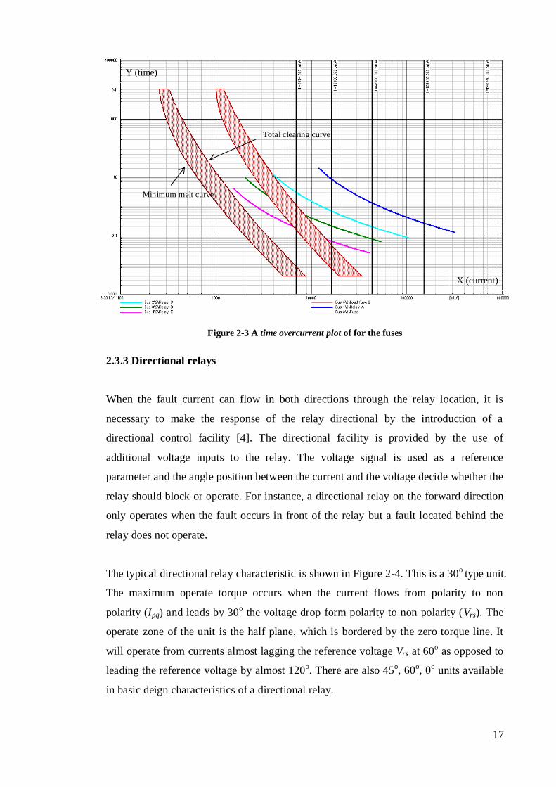
operates. The characteristic curve of a fuse in the time overcurrent plot is given below

in Figure 2-3. This is an example of the distribution network shown in Figure 5-1. The

X-axis represents for the current and the Y-axis represents for the time. Further details

are in the Appendix A.1.3. The Minimum Melt Time (MMT) is the time between

initiation of a current large enough to cause the current-responsive element to melt and

the instant when arcing occurs. The Total Clearing Time (TCT) is the total time

elapsing from the beginning of an overcurrent to the final circuit interruption; i.e. TCT

= minimum melt + arcing time.

17

Figure 2-3 A time overcurrent plot of for the fuses

2.3.3 Directional relays

When the fault current can flow in both directions through the relay location, it is

necessary to make the response of the relay directional by the introduction of a

directional control facility [4]. The directional facility is provided by the use of

additional voltage inputs to the relay. The voltage signal is used as a reference

parameter and the angle position between the current and the voltage decide whether the

relay should block or operate. For instance, a directional relay on the forward direction

only operates when the fault occurs in front of the relay but a fault located behind the

relay does not operate.

The typical directional relay characteristic is shown in Figure 2-4. This is a 30o

type unit.

The maximum operate torque occurs when the current flows from polarity to non

polarity (Ipq) and leads by 30o the voltage drop form polarity to non polarity (Vrs). The

operate zone of the unit is the half plane, which is bordered by the zero torque line. It

will operate from currents almost lagging the reference voltage Vrs at 60o as opposed to

leading the reference voltage by almost 120o. There are also 45

o, 60

o, 0

o units available

in basic deign characteristics of a directional relay.

Total clearing curve

Minimum melt curve

Y (time)

X (current)

18

Vrs30°

Maximum

torque

line

Operate

zone

Zero

Torque

line

Nonoperate

zone

Ipq +

+ I

s r

p

V

Voltage polarized

Directional relay

q

Figure 2-4 Typical directional relay characteristic (30o type unit)

2.3.4 Current and voltage transformer

Current or voltage instrument transformers are essential to isolate the protection, control

and measurement equipment from the high primary currents and voltages of a power

system. Supplying the equipment with the appropriate values of the current and

voltage—generally these are 1 A or 5 A for the current coils, and the 120 V for the

voltage coils. The behaviour of current and voltage transformers during and after the

occurrence of a fault is critical in electrical protection since errors in the signal from a

transformer may cause mal-operation of the relays.

The nominal primary voltage of a VT is generally chosen with the higher nominal

insulation voltage (kV), and the nearest service voltage in mind. The nominal secondary

voltage is generally standardized at 115 and 120 V. In order to select the nominal power

of a VT, it is usual to add together all the nominal loadings of the apparatus connected

to the VT secondary winding. In addition, it is important to take into account the voltage

drops in the secondary wiring, especially if the distance between the transformers and

the relays is large.

Almost all CTs universally have a 5 A secondary rating. Other ratings exist, such as 1 A

but are not common. When selecting a CT, it is important to ensure that the fault level

19

and normal load conditions do not result in saturation of the core and that the errors do

not exceed acceptable limits. The transformation ration of the CTs is determined by the

larger of the following two values [2]: nominal current or maximum short-circuit

current without saturation being present.

2.3.5 Equipment damage curves

When a fault occurs, the equipment will suffer a significant fault current and could be

damaged because of the extremely high current after a prolonged period. Damage can

be thermal or mechanical. As with OC protection, it is usual to plot damage curves of

cables or transformers on a log-log graph along with the relay characteristics. When

assessing the protection system in a network, we should consider that the protection

characteristic curves must be below and to the left of the damage curves of any plant

that they are responsible for protecting [5]. An example of the damage curves can be

seen in Figure 2-5, in the time overcurrent plot, relay F is protecting the cable C 2-6

from probable permanent damage.

Figure 2-5 Example of a cable damage curve

2.3.6 Transformer inrush current

Thermal damage curve

(C 2-6)

Relay F characteristic

Mechanical damage curve

(T133/33)

Relay A characteristic

Y (time)

X (current)

20

When a transformer is energized, a transient current refers to the maximum,

instantaneous input current that can flow for several cycles. The selection of overcurrent

protection devices such as fuses and circuit breakers is made even more complicated

when high inrush currents must be tolerated. The overcurrent protection must react

quickly to overload or faults but must not interrupt the circuit when the inrush current

flows. The duration of an inrush current can only be sustained for a few cycles, while

the breaking time of a protective device usually lasts for several seconds. As long as the

tripping time of protective devices is longer than the duration time of an inrush current,

the false distinguishing problem caused by an inrush current can be eliminated [6].

2.4 Distance protection

2.4.1 Distance relay

Distance relaying can be applied when overcurrent relaying cannot fulfill the protection

requirements such as sensitivity, and selectivity. Distance relays are capable of

measuring the impedance of a line to a reach point and are designed to operate only for

faults occurring between the relay location and the reach point, and thus can distinguish

faults that may occur beyond the protected zone. The reach point of a relay is the point

along the line impedance locus that is intersected by the boundary characteristic of the

relay [4]. As this is determined by the division of the voltage and current and phase

angle, it is plotted on an R-X plot for a clear observation.

2.4.2 Types of distance relays

Distance relays are classified depending upon their characteristics in the R-X diagram,

where the resistance R is the abscissa and the reactance X is the ordinate. Under any

circumstance the origin is the relay location and the operating area is usually in the first

quadrant. Whenever the ratio of the system voltage and current fall within the circle

shown, or in the cross-hatched area, the unit operates [6].

Typical characteristics of the distance relays on these axes are displayed in the

following figures. Figure 2-6 shows two distance relay characteristics, the left diagram

is impedance characteristic. The impedance characteristic will operate in all the 4

quadrants. This design needs an extra directional-sensing unit since it operating in all

http://en.wikipedia.org/wiki/Fuse_(electrical)

http://en.wikipedia.org/wiki/Circuit_breaker

http://en.wikipedia.org/wiki/Short_circuit

21

four quadrants. Thus, this type is obsolete design. The MHO characteristic is a circle

whose circumference passes through the origin, which combines the properties of

impedance and directional relays. This states that the impedance element is inherently

directional and, therefore, it will operate only for faults in the forward direction.

jX

R

jX

R

Figure 2-6 Distance relay characteristics on the R-X diagram

An MHO distance relay requires the voltage to operate correctly. However, the voltage

will be very small or approaching zero for a fault right at the relay location. If the

voltage falls to zero during a fault, the tripping of the relay could be inoperative or

inactive. For a three-phase close-in fault, the operation of any of the MHO functions

may be jeopardized because there will be very little, or no voltage available to develop

the polarizing quantity [7]. A memory circuit may be used to prevent the immediate

decay of voltage applied to the relay terminals when a three-phase short-circuit occurs

close to the relay bus [4].

2.4.3 The effect of arc resistance on distance protection

The impedance measured by a distance relay is made up of resistance and inductance up

to the fault point. Nevertheless, the fault may involve an electric arc or an earth fault

including additional resistance. The impedance angle is then affected by the value of the

resistance of fault impedance, which might result in the total resistance seen by the relay

outside the characteristic or the circle. Thus a relay characteristic with an angle setting

equal to the line angle will have an under-reach problem. It is common to set the relay

characteristic angle a little less than the line angle in order to accept a small amount of

fault resistance without producing under reaching.

22

Figure 2-7(a) shows the effect of arc resistance on the MHO relay. R is the arc

resistance and Zf is the impedance of the line up to the fault point F. The relay

characteristic angle is equal to the line characteristic angle µ. For a fault at F, the

impedance measured by the relay is Zf + R and is outside the characteristic circle. This

displays the arc resistance and causes under reaching. If the MHO characteristic is

shifted, the characteristic angle α of the MHO relay will be less than the angle µ in

Figure 2-7 (b). In this case, the impedance Zf + R measured by the relay remains within

the characteristic circle. The characteristic angle of the relay is less than the

characteristic angle of the line and could have a greater tolerance for the arc resistance.

jX

µ

F

Zf

R

Zl

Zf +R

jX

Zl

F R

Zf

Zf +R

α µ

(a) (b)

Figure 2-7 The effect of arc resistance on the MHO relay

2.5 Chapter summary

Basically, a protection system is made up of instrument transformers, protection relays,

circuit breakers and auxiliary power supplies. The suitable protective devices (current

transformer, voltage transformer, overcurrent relays, directional relays, distance relays,

fuses etc.) are selected for different networks. In the meantime, each protective device

should be considered in details regarding pick-up current settings, characteristic curves,

the reaching of a protection zone, etc. When considering protective devices, some

noticeable issues (such as equipment damage curves, the arc resistance) are discussed as

well.

23

3. Protection coordination


This chapter describes what protection coordination involves and how to coordinate the

protective devices in different network topologies.

The protection coordination problem is about determining the sequence of relay

operations for each possible fault location and to provide sufficient coordination

margins without an excessive time delay [8]. Coordination margin or coordination

grading or coordination time interval is the time delay between the operation of the

main and the back-up protective devices. Its value is, usually 0.2-0.5s. As mentioned

before, all protective device settings in the network must be carefully calculated to

ensure that the coordination between protective devices is successful. A relay only trips

the circuit breaker in situations when the fault location is within its protection zone. It is

essential that any fault is efficiently isolated, thus, wherever possible, every element in

the power system should be protected by both primary (main) and back-up relays. If a

fault occurs, the main protection should trip the circuit breaker instantaneously. After

that, after a time delay (coordination margin), the back up protection should operate if

the primary protection does not respond properly.

3.2 Overcurrent protection coordination in different network configurations

3.2.1 Basic overcurrent protection coordination rules

The basic rules for a correct overcurrent relay coordination can generally be stated as

follows [4]:

a) Whenever possible, use relays with the same operating characteristic in series with

each other

b) Make sure that the relay remotest from the source has a current setting equal to or

less than the relays behind it, that is, the primary current required to operate the

24

relay in front is always equal to or less than the primary current required to operate

the relay downstream it

The coordination of time overcurrent relays is the process of determining settings for

the relays that will provide a proper protection operation in case of a fault [8]. IDMT

characteristics are the most widely used where grading is possible over a wide range of

currents and relay can be set to any value of definite minimum time required. The

selection of settings will now be explained in detail.

There are two main settings that need to be considered when using IDMT relays:

the pick-up current and the time multiplier setting (TMS). These are discussed in

Section 2.3.1. The pick-up current is the threshold that indicates the minimum operating

current for the IDMT relay. The current setting must be chosen so that the relay does

not operate for the maximum load current in the circuit being protected, but does

operate for currents equal or greater than the minimum expected fault current. The TMS

is applied to ensure the coordination between protective devices, providing a family of

curves so that two or more relays sensing the same fault current can operate at different

times [6]. The time interval that must be allowed for the operation of two adjacent

relays to achieve correct discrimination between them is called the grading margin [6].

Usually the same grading margin will be applied across the entire protection system,

which is normally 0.25s for numerical protection relays.

The coordination of the overcurrent scheme starts with the remotest downstream device

and then is coordinated with each upstream device back towards the source.

Downstream means the point is further away from the source and upstream means the

point is close to the source. Devices are coordinated by the combination of the current

and the time. A practical and effective method for verifying the protection coordination

between protective devices is to analyze the time-overcurrent curves of devices.

3.2.2 Overcurrent protection coordination in radial network

Conventional OC protections normally have radial topology, which is characterized by

a utility source at the upstream side; therefore, the fault current has only one direction,

this direction is from an upstream single source to the downstream fault point. The

selectivity of a protection system can be clearly observed in the time-current diagram of

a radial network with a single resource. A relay close to the fault point operates in the

25

largest fault current, and a relay near to the source operates in the shortest operating

time. Thus for a particular fault, all the relays connected in the radial feeder see the fault

current but are set to operate at different times by selecting different time current

characteristics [9].

For instance, consider Figure 3-1, a radial network with only one source that supplies

the power system. This is a simplest configuration and the selectivity can be easily

achieved. Relays A, B, and C used to protect the network are OC IDMT relays. The

selection of the upstream relay B needs to be coordinated with the downstream relay C

and the grading between two relays will take place at the maximum fault current at line

C-D. For a fault at line C-D, relay C should trip first as the main protection and relay B

works as a back-up protection and has a higher TMS. If relay C fails to operate, relay B

will trip after a time delay (grading margin). After selecting the appropriate IDMT

characteristic curve for relay B, the same procedure should be repeated for the

coordination between relay B and relay A.

t

A

IDMT relay C

IDMT relay B

IDMT relay A

Max fault Line C-D

Max fault Line B-C

Grading margin

Grading margin

Relay A Relay B Relay C

Bus A Bus B Bus C

Max fault line C-DMax fault line B-C

Figure 3-1 The coordination of IDMT relays

26

3.2.3 Protection coordination in networks with multiple sources

A distribution network can be supplied by multiple sources to increase the reliability of

power supply for customers. Nevertheless, it also costs more and makes the protection

consideration more demanding. In the network supplied by two sources (see Figure 3-

2), the network should be protected by directional OC relays. The vertical axis (T)

represents time and the horizontal axis (L) shows the relative distance from relay to the

source. If E2 does not exist, then the tripping sequence of relays 1, 2 and 3 would be the

same as in the case with a single source E1. If relays 1, 2 and 3 are directional OC

relays and they only trip when the fault current flows into the line, then the coordination

procedures for OC relays mentioned before can be used here to achieve the proper

coordination between relays 1, 2 and 3. The coordination between relays 4, 5 and 6 is

the same, but now E1 should be ignored and relay 1 is the farthest remotest downstream

from E2 and should be set first. In the network with two sources, we need to repeat the

coordination procedures twice and they are independent of each other. The second

diagram represents the tripping sequence for relays in the network below.

For instance, if a fault occurs between relay 3 and relay 4, relay 3 will trip first to break

the fault; if relay 3 fails, then relay 2 will trip with a time delay; the final relay which

has the longest tripping time is relay 1 and the fault will be disconnected from source

E1 if any of them have tripped. At the same time, relay 4 has to disconnect source E2 as

well.

Figure 3-2 Coordination in a multiple sources system

Relay 1 Relay 2 Relay 3 Relay 4Relay 5Relay 6

A B C D

E1E2

T

L

L

T

t1

t2

t3

t4

t5

t6

27

3.2.4 Protection coordination in meshed networks

With the fast growing expansion of modern power systems and the high demand for

power supply quality, the meshed network with multi resources is becoming a hot spot.

A meshed network can have one close-loop or several close-loops and are much more

complicated than a radial network. The diagram below is an applicable loop network

and shows how to coordinate such a network configuration.

For a special meshed network (ring or close-loop network) displayed in Figure 3-3,

there are 3 sources that provide the fault current. One is an external grid and the other

two are asynchronous machines. Directional overcurrent (OC) relays are necessary in

the system with multiple sources. There are six directional OC relays with IDMT

characteristics installed at both ends of the line. Each directional unit will operate when

the current flows into the line section.

Relay 1 Relay 2

Relay 3 Relay 4 Relay 5 Relay 6

Bus A

Bus B Bus C

Figure 3-3 A meshed network with multiple sources

28

Relay 3 Relay 1 Relay 2 Relay 3

Bus C Bus A Bus B Bus C

CTI CTI CTI

Figure 3-4 Coordination between directional IDMT relays around clockwise

In setting relays around a loop, a good general rule is to attempt to set each relay to

operate in less than 0.2s for the close-in fault and at least 0.2s plus the CTI

(coordination time interval) for the far-bus fault [6]. A fault close to relay is known as

close-in fault for the relay and a fault at the end of the line is know as far-bus fault for

the relay. Taking Figure 3-4 for example, the tripping time takes longer when the fault

current decreases. The IDMT characteristics of each relay are a curve which indicates

that the tripping time takes longer when the fault location is far from the relay. Relay 1

should coordinate with relay 3 as the main protective device for the fault between bus A

and bus B, and should coordinate with relay 2 as the back-up protective device for the

fault between bus B and bus C. Relay 1 coordinates with relay 3 for the close-in fault

formula and it coordinates with relay 2 for the far-bus faults restraint. This is the same

procedure and requirement for relay 2 and relay 3. Further information regarding the

explanation can be found in [6].

3.3 Distance protection coordination

The protection of a distributed network becomes challenging once the amount of

generation has increased, which may be either directly connected to the network, or

indirectly connected to the network, i.e. through step-up transformers. Specifically,

prospective fault currents can vary over a wide range, and may become bi-directional.

This causes the grading of the overcurrent relays very difficult [10]. This difficulty

applies equally to radial circuits protected by directional relays. Furthermore, to

maintain the stability of distributed generators, fault clearance times should be kept to a

minimum [11]. The characteristics of a distance element can be shaped and distance

relays are inherently directional. Moreover, a distance relay installed can make the OC

element directional with a distance element providing the torque control [12]. Distance

protection can enhance the performance, with or without a DG connected.

29

The protection coordination becomes more complex and varied with the introduction of

distance relays to the network. Without distance relays, one simply takes the

coordination between OC relays into consideration. However, after the distance relays

are employed in the protection system, the coordination between the distance relays and

the coordination between the distance relay and the OC relay must be taken into account.

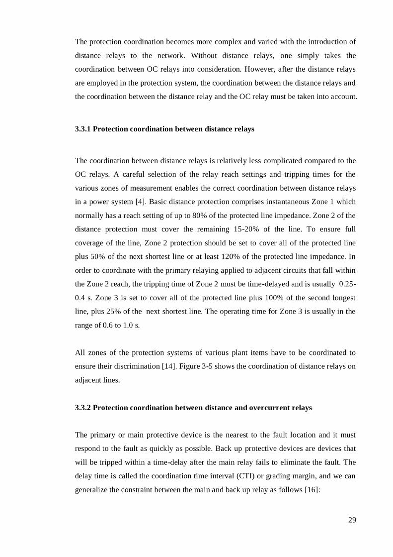
3.3.1 Protection coordination between distance relays

The coordination between distance relays is relatively less complicated compared to the

OC relays. A careful selection of the relay reach settings and tripping times for the

various zones of measurement enables the correct coordination between distance relays

in a power system [4]. Basic distance protection comprises instantaneous Zone 1 which

normally has a reach setting of up to 80% of the protected line impedance. Zone 2 of the

distance protection must cover the remaining 15-20% of the line. To ensure full

coverage of the line, Zone 2 protection should be set to cover all of the protected line

plus 50% of the next shortest line or at least 120% of the protected line impedance. In

order to coordinate with the primary relaying applied to adjacent circuits that fall within

the Zone 2 reach, the tripping time of Zone 2 must be time-delayed and is usually 0.25-

0.4 s. Zone 3 is set to cover all of the protected line plus 100% of the second longest

line, plus 25% of the next shortest line. The operating time for Zone 3 is usually in the

range of 0.6 to 1.0 s.

All zones of the protection systems of various plant items have to be coordinated to

ensure their discrimination [14]. Figure 3-5 shows the coordination of distance relays on

adjacent lines.

3.3.2 Protection coordination between distance and overcurrent relays

The primary or main protective device is the nearest to the fault location and it must

respond to the fault as quickly as possible. Back up protective devices are devices that

will be tripped within a time-delay after the main relay fails to eliminate the fault. The

delay time is called the coordination time interval (CTI) or grading margin, and we can

generalize the constraint between the main and back up relay as follows [16]:

30

(3-1)

where and are the operating times of the backup and main relays respectively.

The derivation of the coordination arrangement for the systems where the OC and the

distance relays are installed is discussed with the aid of Figure 3-6. There are two

important constraints [15]-[16].

Zone 1 = 80% Zone 1 = 80%

Zone 1 = 80%

Zone 2 > 120%

Stat A

Stat A

Stat B

Stat A

Stat B

Stat C

Stat C

Time

Distance

Figure 3-5 Coordination between distance relays

Tb

F1 F2

Tm

Tz2

>CIT

>CIT

Tz2

Backup Main

t

Distance

Figure 3-6 Coordination between distance and OC relays

a. The second zone backup distance relay must be slower than the OC main relay,

which can be stated as follows:

31

(3-2)

b. The OC backup relay must be slower than the second zone of the main distance

relay:

(3-3)

is the operation time of the OC relay and is the operating time of the second

zone of the distance relay. It indicates that both types of relays are taken into account.

Constraints show that: if a fault occurs, the main relay should operate faster than the

backup relay. In Figure 3-9, if the primary protection (main OC relay or Zone 2 of the

main distance relay) could not break the fault at F2, the backup OC relay should trip

after a determined grading margin, or CTI. For a fault at F1, if Zone 1 of the main

distance relay or the main OC relay is unable to clear the fault, Zone 2 of the backup

distance relay or the backup OC relay should operate to clear the fault after a CTI. Some

examples of CTI are shown in Figure 3-6 in the time overcurrent plot and also in Figure

3-1.

3.4 Chapter summary

In conclusion, the protection coordination ensures a faster pick-up time of protective

devices; it minimizes the interruption time; it ensures that only the faulted elements are

disconnected from the system and it keeps the healthy items unaffected in a protection

scheme. In different protection schemes and network configurations, the coordination

procedures and consideration are not the same. This Chapter provided detailed

explanation on how to coordinate between overcurrent relays in radial networks, radial

networks with multiple sources and meshed networks. Moreover, the procedures of

protection coordination between distance relays and the rules and formulas of how to

coordinate between distance relays and overcurrent relays were discussed as well.

32

4. Impacts of renewable energy sources on protection

coordination


Most Distributed Generators (DGs) are defined as renewable energy, green energy

sources and are gradually being utilized to provide a power supply for conventional

distribution networks. Distributed generators are made up of induction and synchronous

machines. Loss of the power source to the circuit to which an induction generator is

connected will normally cause the generator to shut down. The induction generators can

not usually become self-excited because they do not have a separate excitation system.

A source of excitation current for magnetizing is required for the stator to induce rotor

current. There is no sustained fault current as an induction generator draws its

magnetizing current from the network. Thus, they are not capable of supplying isolated

loads or sustained fault currents when separated from the power system [27]. The usage

of DGs not only gives advantages to electricity users, but it also brings benefits to

utilities. The merits of the application of DGs can be summarized as: increased voltage

stability, loss reduction and high efficiency, environmental concerns and low pollution

[17]-[19].

The purpose of protection coordination is to decide the sequence of relay trips and to

ensure acceptable coordination grading margins without excessive time delay. DG

connections will have a significant influence on the protection coordination. When DGs

are connected to the main grid, the protective devices connected will detect different

fault current levels and sense the fault current flow in more than one direction. A

summary of the influence of DGs on the network, in terms of coordination problems, is

given in the following chapter.

4.2 False tripping of overcurrent relays

In an active distribution network, both DGs and the external source will be subject to a

fault current, whereas in a passive distribution network the fault current flows only from

a single resource. Hence, a protective device located in the DG feeder in an active

network may see a fault current flow from the DG caused by faults elsewhere in the

33

system. To illustrate this problem in Figure 4-1, there are two sources supply the

network, one is an external grid, another is a distributed generator. The relay A should

trip for a short-circuit fault on the adjacent feeder 1; however, the relay B will see the

fault current as well and may cause false tripping and then disconnect the non-faulted

feeder 2. A solution to this problem, as stated in [20]-[21] is to apply directional relays

to protect the feeders that may bring about false tripping. .

Relay AGrid

Relay B

1

2

DG

I1

Ig

Figure 4-1An illustration of a situation where false tripping may occur

4.3 Loss of protective devices grading

The current injected by DGs will change the fault level both in magnitude and direction,

which thereby results in a loss of selectivity. The protective devices are designed to

sense a certain minimum fault current, which normally includes the ends of the feeder.

As the penetration of the DG increases, it is more difficult to detect or sense a fault in

overcurrent devices with the settings that were based on the minimum fault current

before the DGs was connected. Additionally, the coordination margin is also used to

distinguish the operating time of the relays. With more DGs installed out on the feeder,

they will cut into the margin [22]. The problem can be resolved by readjusting the

settings of the OC relays to build the new grading margin and to acquire the appropriate

relay characteristics.

4.4 Blinding of overcurrent relays

When a DG is downstream of a relay and upstream of the fault point, the DG will

contribute to the total fault current, but it will decrease the fault current seen by the

relay at the same time. This may cause delayed tripping of the relay and could,

34

potentially, in the worst scenario lead to the non-tripping of the relay. This problem is

referred to as “Blinding of OC protection” [21]-[24].

Figure 4-2 displays a simple network with or without DG connection. Ir is the fault

current sensed by the relay and If is the fault current flow into the fault location. Without

the DG connected,

. With the DG connected:

,

. These equations show that the

total fault current is increased and the fault current seen by the relay is decreased with

the DG connected.

Relay

DG

Ir

Ig

If

Ir(1)

If(1)

Without DG connected

ZrIr(2)

If(2)

With DG connected

Figure 4-2 An example of blinding

The most straightforward method to avoid such a problem is to reduce the tripping time

in order to assure correct operation, despite the blinding. A definite-time OC protection

characteristic operates with a fixed time delay; when a definite-time characteristic is

used there is no risk of binding because the tripping time is fixed no matter how the

fault current changed. On the contrary, the operating time of IDMT characteristics will

change as the fault current value varies. Therefore, a combination of an IDMT and a

definite-time OC relays can be employed to tackle this difficulty. The following time

overcurrent plot (Figure 4-4: T means time, I means current) demonstrates the

characteristics of relay A and relay B. Relays A and B are both IDMT overcurrent

relays. The coordination margin between relay A and B will obviously shrink after the

definite-time characteristic has been introduced in relay A.

35

Relay AGrid Relay B

DG

I

T

Grading margin

between IDMT

characteristics

Grading margin

between IDMT and

definite time

characteristics

IDMT characteristic

(relay A)

Definite time

characteristic

(relay A)

IDMT characteristic

(relay B)

Figure 4-3 An example solution for the blinding problem

4.5 The effect of infeed on the distance protection

On the basis of the impedance measured, distance relays have the advantage that they

can distinguish faults in different parts of a network. Essentially, this involves

comparing the fault current, as seen by the relay, against the voltage at the relay location

to determine the impedance down the line to the fault [15]. The effect of infeed needs to

be taken into account when there are one or more generation sources within the

protection zone of a distance relay which can contribute to the fault current without

being seen by the distance relay [1].

Analysing the case presented in Figure 4-1, it can be seen that the actual impedance to

the fault is + , but when the current flows, the impedance appears to the relay as

+ + ⁄ ) . The impedance seen by the distance relay for a fault beyond busbar

B is greater than what actually occurs. This effect is called the “infeed effect”.

36

The presence of the DG can cause the “infeed effect”. When DGs are added to the

distribution network, the fault current from the generation adds to the fault current from

the utility [26]. In Figure 4-3, if the current flows from the DG connected to bus C,

the distance relay may not operate according to its defined zone as the relay sees the

impedance influenced by the DG as well as the infeed current.

A B

Relay

IA IB+IA

ZA

ZB

IB

Fault

DG

C

Figure 4-3 Example of infeed effect

The influence of the DG is the reduction in the reach of the distance relay, which can be

summarized in as follows [26]: “When a fault occurs downstream of the bus where the

DG is connected to the utility, the impedance measured by an upstream relay will be

higher than the real fault impedance.”

Due to the penetration of DGs, the setting of Zone 2 and 3 for the relay should then take

the following form:

(4-1)

where K, the infeed constant, is given as:

Since the value of the infeed constant depends on the zone under consideration, several

infeed constants, referred to as , and , need to be calculated. is used to

calculate the infeed for Zone 2. and are used for Zone 3. takes into account the

infeed on the adjacent line and that in the remote line [2]. The calculation process in

detail can be found in [2].

37

As far as the under reach problem (distance relay) is concerned, readjustment of the

relay setting for each zone can make the relay operate correctly. The influence on zone

reaching, caused by the DG, can be minimized or eliminated through a careful

calculation process that considers the infeed constant. An adaptive distance scheme for

the distribution system with DG can be found in [26]. This method focuses on the value

settings of Zone 2 based on protected characteristics.

4.6 Chapter summary

As a result of the penetration of the DGs in distributed networks, some problems (false

tripping, loss of grading, blinding, the effect of infeed) related to protection

coordination have arisen. Through a proper design of the protection concept and

protection coordination, each of these issues can be solved. Loss of grading margin is an

inevitable issue when it comes to protection coordination and necessary readjustment is

needed. In terms of overcurrent relays, false tripping and blinding problems could affect

the sensitivity and selectivity of the protection system. The solution is to adopt

directional overcurrent relays to prevent the circuit from potential false tripping. As for

blinding of overcurrent relay, a combination of IDMT and a definite time characteristics

is the solution. The effect of the infeed current could result in under reaching of the

protected zone, which should be taken into account when studying the coordination

between distance relays.

38

5. Computer simulation faulted distribution networks using

DIgSILENT


The purpose of this chapter is to focus on how to use DIgSILENT to simulate faulty

networks and to demonstrate the selection of setting and operation of protection

systems. In this chapter the medium voltage (MV) network adopted from [27] will be

employed to illustrate the protection coordination procedures with the help of two

possible DIgSILENT networks:

1. radial network without DGs

2. distribution network with DGs

5.2 Network modeling

The power system software called DIgSILENT PowerFactory [25] can be applied to

simulate and analyze the protection system of a network. By using a single database,

containing all the required data for all the equipment within a power system (e.g.

transmission lines data, cables data, generator data, protection data, signal distortions

data, controller data), PowerFactory can easily execute a number of network planning

applications. Some of these applications are load flowing, short-circuit calculations,

harmonic analysis, protection coordination, stability calculations and model analysis

[25]. The PowerFactory protective devices are all stored in the cubicle connected to the

busbar and branch element, with CTs, VTs, circuit breaker and relays. Further

information regarding the software is given in Appendix 1.

The 132 kV, 50 Hz external grid supplies the system through a 132/33 kV/kV

transformer (see Figure 5-1). All loads are both static and balanced and their total

loading is 28.1 MW. In the simulation, a large wind farm will connect to bus 2 through

a T33/11 kV/kV transformer and a small wind farm will integrate to the system (bus 3)

directly. All circuit breakers are stored in the same cubicle where relays locate in.

39

The large wind farm (See Figure 5-2) has six 11 kV strings and is comprised of 30 wind

turbines, while the small wind farm (See Figure 5-3) contains two strings, and 10 wind

turbines. Both of them are modelled using an induction machine as the wind turbine

(0.96 kV, 1200 kVA) and each string is composed of five turbines. Each turbine is

connected to the 11 kV collection busbar via the 11/0.69 kV transformers.

Bus 1

132 kV

Bus 2

33 kV

Bus 3

11 kVBus 4

11 kV

Bus 5

3.3 kVT33/11 T11/3.3

Relay A

I>

51

Relay C

I>

51

51N

Relay F

I>

51

51N

Fuse

Fuse

Fuse

Fuse

Fuse

Fuse

Relay D

I>

51

51N

Relay E

I>

51

51N

T132/33

External grid

3500 MVA

Load 1Load 2Load 3

Load 4

Load 5

Load 6

Figure 5-1 Singe line diagram of the distribution network without DGs

Bus 1

132 kVBus 2

33 kV

T132/33

3500 MVA

G G G G GG

WT 1 WT 4 WT 5 WT 56WT 59 WT 60

Large wind farm

11 kV

T33/11

T11/0.96

11 kV

0.96kV

To the rest of

the network

Figure 5-2 Singe line diagram of the large wind farm

Bus 3

11 kV Bus 4

11 kV

Bus 5

3.3 kVT11/3.3

Fuse

FuseLoad 2Load 3

GG

GGLoad 1

WT 1

WT 5

WT 6

WT 10

Small wind farm

11 KV

To the rest of

the network

11 kV

0.96kV T11/0.96 Figure 5-3 Singe line diagram of the small wind farm

40

5.3 Protection coordination in a MV network prior to the DGs connection

The overall single line diagram of the network with protection devices installed in the

radial network was connected is shown in Figure 5-1. Overcurrent protection has been

used to protect the radial network.

The coordination of time overcurrent relays is the process of determining settings for

the relays that provide a selective response for a fault [8]. PowerFactory has provided

users the application for protection analysis. For example: different relay types

(direction, distance, OC) are available for use in the Global Library, the calculation of

fault current is applicable. On the basis of the protection system feature, the proper

protection system is selected on. In this network, the overcurrent protection devices

(fuses, OC relays) are explained and more information regarding other types of

protection can be found in the DIgSILENT user’s manual [25].

5.3.1 Selecting protective devices

The main and the back-up protection across the network are comprised of the OC phase

and earth faults protection that are selected from the Global Library. Loads are initially

protected by fuses. All OC relays used to protect the radial network are set based on the

basic rules for correct relay coordination (as described in Section 3.1). Specifically,

relays selected in this case are numerical relays (IAC77A805A) that have a phase and

an earth OC element, and both follow an Extreme Inverse (EI) Characteristic (IAC

Extreme Inverse (EI) GES7005B). The reason for choosing the EI characteristic is

because relays must be properly coordinated with their downstream fuses. Due to the

HV delta connection of all transformers in the network, earth faults occurring at the LV

winding of the transformer will not result in zero sequence current flowing on the HV

side. Therefore, if a transformer is located in the middle of two relays, the phase

element of the upstream relay must be able to provide the back up protection for the

earth element of the downstream relay.

Without doubt, the OC relays require a three-phase current transformer to deliver an

input signal for both the phase and earth faults. The secondary nominal current of the

CT setting in this network is 5A. The C100 core CTs are used and the total burden for

each CT is 1 Ω; the selection of proper CTs ratio can be found in Section 2.2.4.

41

5.3.2 Pick-up currents of relays and fuses

After selecting the appropriate protective devices for the network, the next stage is to

calculate the pick-up current of the OC relay; the phase and earth element need to be

calculated and set separately. The relay settings should be calculated by the shortest

operating time according to the maximum fault current and the setting should be

sensitive enough to pick up when the minimum expected fault current occurs. The OC

relays do not provide an overload protection as their responsibility is to separate faulted

zones from the network; therefore, the relay pick-up current setting must be greater than

the maximum load current to prevent mal-operation. The fuses adopted are both of the

medium voltage type in DIgSLIENT and the rated frequency is 50 Hz. The settings are

explained in Section 2.2.2. The overall fuse data are provided in the Table 5-1 below.

Fuse Rated voltage (kV) Rated current (A)

Load fuse 1 11 224

Load fuse 2 4 200

Load fuse 3 4 200

Load fuse 4 33 200

Load fuse 5 33 200

Load fuse 6 33 200

Table 5-1 Fuse data

5.3.3 Explanation of the protection coordination

A time-overcurrent plot is comprised of the characteristic curves of relays and fuses

from which the pick-up current, short circuit values, TMS and grading margin can be

read. Further details are in the Appendix A.1.3. The coordination procedures between

IDMT relays use a time-overcurrent plot, which has been pointed out previously (as

described in Section 3.2.2, Figure 3-1). In a large system like this, the calculation of

protection settings could be enormously complicated. Fortunately, DIgSILENT can be

used to help with the calculation and process. The method used in this case is to

manually adjust the relay characteristic curves or to reset the settings of each curve in

the time-overcurrent diagram provided by DIgSILENT. The diagram allows the

coordination between the two devices to be done graphically as well, by moving their

characteristics (Section A.1.3).

42

Figure 5-4 below as shows an example for adjusting the relay characteristic curves: the

original characteristic is labelled "1'', the new position as "2'', and the grading margins

are labelled "a''. The proper coordination margin between relays can be done through

this method. In this network, the grading margin is at least 0.2s because the numerical

OC relays were installed in the protection system and they could deliver a faster

response in case of a fault.

Figure 5-4 Moving characteristic showing the grading margin

Figure 5-5 The phase element of relay characteristics in the time overcurrent plot

Y (time)

X (current)

43

In Figure 5-5, the time overcurrent plot, where the characteristics of the phase element

of OC relays from bus 5 to bus 1 are shown. Clearly, the coordination between all relays

and fuses from downstream to upstream can be observed from the plot. The

characteristic curve of the protective device (load fuse 2) that is furthest from the source

is displayed in the plot on the furthest left. Whereas, the characteristic curve of the

nearest protective device from the source is shown in the plot on the furthest right

(Relay A).

5.3.4 Equipment damage curves and inrush current

As mentioned already in Section 2.2.5, the equipment damage curves and transformer

inrush current also need to be emphasized when plotting the relay characteristic curve.

The protection characteristic curves of the relays must be set below and to the left of the

damage curves of any plant that they are responsible for protecting. For instance, the

acceptable protection for transformer T132/33 from both thermal and mechanical

damage is provided by relay A in Figure 5-6. Moreover, through the assessment of the

inrush current, it is clear that the tripping time of relay A is longer than the period of the

transformer inrush current, as shown in Figure 5-6. As a result, relay A can tolerate the

inrush current and not interrupt the circuit.

Figure 5-6 Example of transformer damage curve and inrush current

Mechanical

damage curve (T133/33)

Thermal

damage curve

(T133/33)

Relay A

Inrush current

X (current)

Y (time)

44

5.3.5 Relay parameters

The protection system for the radial network and the protection coordination between all

protective devices is successfully achieved through proper adjustments. Figure 5-7 is

the list of settings for all protective relays (relays A, C, D, E, F) in the radial network

without DGs. The list is given by DIgSILENT and the protection coordination is

succeeded according to these settings. For example, see the settings for the relay A in

Figure 5-7, the relay type is IAC77A805A; the ratio of current transformer that is

connected to the relay A is 1000A/5A; the pick up current is 1 A and the time dial

(TMS) is 4, the characteristic is Extremely Inverse (EI), for the phase element of the

relay A. The same information can be read for the earth element of relay A as well.

45

Figure 5-7 Relay parameters with the DG connected

5.3.6 Assessment of different fault cases

After the appropriate selection and the setting of protective devices, and the right

displacement of characteristic curves, different fault situations have been studied.

In the first scenario, a single phase fault at 50% C-load 4 near bus 6 will be

cleared by the fuse 4 after 0.022s. If fuse 4 fails to operate, then the relay C2 will

respond after 0.332s. (Figure 5-8)

Another short circuit situation at cable C 3-4 is a three phase balanced fault. Skss

(The capacity of the short circuit) is 139 MVA, Ikss (The value of the short circuit) is

7.3 kA is. It will be cleared by main protective relay D (0.137s) or by the back-up relay

C (0.4s). (Figure 5-9)

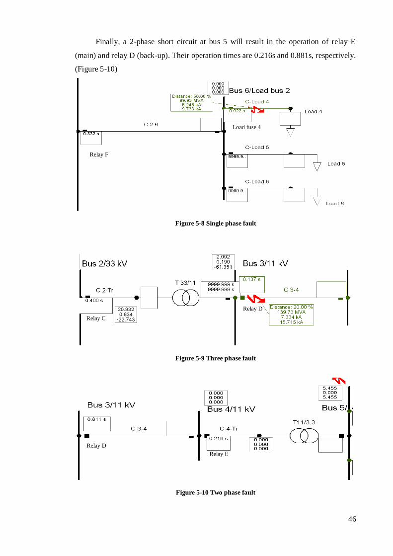
46

Finally, a 2-phase short circuit at bus 5 will result in the operation of relay E

(main) and relay D (back-up). Their operation times are 0.216s and 0.881s, respectively.

(Figure 5-10)

Figure 5-8 Single phase fault

Figure 5-9 Three phase fault

Figure 5-10 Two phase fault

Relay F

Load fuse 4

Relay C

Relay D

Relay D

Relay E

47

5.4 Protection coordination in a MV network with DG connected

The protection system designed for the radial network has acquired the protection

coordination requirements. Then the additional DGs are connected to the radial network,

which result in the reconsideration about the protection system. There are two wind

farms integrated in the MV network. As we can see from Figure 5-11, After the DGs

have been connected, additional DG OC directional protection must also be provided

(red color in Figure 5-11). The OC directional protection protects the utility system

from harm caused by the DG, and it also serves to protect the DG from events that may

originate in the utility system. The protection system is divided into two parts, one part

is OC directional protection and the other part is main network protection.

The directional OC relays should be installed at every busbar (located in the red part of

Figure 5-11). The coordination procedures of directional OC relays are employed as

mentioned in Section 3.2.3. In the meantime, attention needs to be paid to the proper

coordination between the OC directional relays and the OC relays located in the main

network.

As for the main network, now that the power comes from multiple sources, part of the

main network may detect different fault currents and fault directions. The OC relays

located in the cables that see fault currents flow from more than one source should be

replaced by directional OC relays (relay A, relay B, relay C, relay D1a).

48

Bus 1

132 kV

Bus 2

33 kVBus 3

11 kV

Bus 4

11 kV

Bus 5

3.3 kVT33/11 T11/3.3

Relay A

Idir>

67

67N

Relay C

Idir>67

67N

Relay F

I>

51

51N

Fuse

Fuse

Fuse

Fuse

Fuse

Relay D1b

I>

51

51N

Relay E

I>

51

51N

T132/33

3500 MVA

Load 2Load 3

Load 4

Load 5

Load 6

G G G G GG

GG

GG

Load 1

Relay D1a

Idir>67

67N

Relay SWa

Idir>67

67N

Relay SWa1

Idir>67

67N

Relay SWb

Idir>67

67N

Relay SWc

Idir>67

67N

Relay LW2a

Idir>

67

67N

Relay LW1a

Idir>67

67N

Relay LW1b

Idir>67

67N

Relay LW2b

Idir>67

67N

Relay LWc2

Idir>67

67N

Relay LWc1

Idir>67

67NRelay LWd2

Idir>67

Relay LWd1

Idir>67

WT 1 WT 4 WT 5 WT 56WT 59 WT 60

WT 1

WT 5

WT 6

WT 10

Large wind farm

11 kV

Small wind farm

11 kV

T33/11 T33/11

Relay B

Idir>

67

67N

Figure 5-11 Overall diagram of the protection system after DG integration

A planning process that properly coordinates the protective devices after the

proliferation of DGs is presented in the flow chart in Figure 5-12. As stated before in

Section 2.2.5, the equipment curves of components need to be re-checked after the

penetration of the DGs. In order to cope with the different situations observed, the relay

settings might be changed to assure the correct thermal limits. After this, the operation

of protective devices must be studied in different fault situations. The study into the

operation of protective relays related to sensitivity problems was normally based on the

smallest fault current. The 2-phase fault that occurs at the electrically furthest point

dictates the smallest potential fault current. Furthermore, in the event of a fault on the

adjacent feeders, there should not be any protective devices tripping in the non-faulted

feeder. It is necessary to follow the flow chart process and to adjust relay settings until

the appropriate coordination has been acquired with the DGs connected to the network.

When checking the operation of a protection system, there are three main influences

mentioned before and the following sections give the specifications in detail.

49

Figure 5-12 Flow chart on the coordination process after DG connection

5.4.1 Loss of grading

First of all, the impact on the grading margin of the main network should be considered.

Before the DGs penetration, the coordination in the main network (black part in Figure

5-11) was successfully achieved. However, the coordination margin was cut off after the

DG integration. The simulation carried out by DIgSILENT detected and recorded the

problems. Figure 5-13 shows that 3-phase fault occurred near bus 5 and was cleared by

the fuse after 0.019s and the back-up relay E after 0.216s. Nonetheless, it is clear in the

Initial values for new DG unit

and connection point

Power flow and short circuit calculations

Check thermal limits

of components

Operation of the

protection system,

Selectivity? Sensitivity?

Proper coordinated

protection

Network

reinforcements

or changes in

the DGs unit

Not ok

Not ok

Not ok Not ok The settings of

relays change

50

second diagram that the small wind farm connected to bus 4 has injected more fault

current: Ikss increased from 6.297 kA to 6.984 kA. The selectivity of the protective

device failed: the back-up relay disconnected the circuit after 0.186s and the

requirement for a coordination margin was not achieved (in this protect, the

coordination margin is at least 0.2s).

The coordination procedures in Section 3.2.3 were repeated until the proper

coordination was achieved in the main network again. In order to check whether

protection coordination has been acquired properly, it would be necessary to test for key

faults (the minimum fault current, the maximum fault current) instead of simply

observing the time overcurrent plot. In a time overcurrent plot of a single source

network, relays see the same fault current in a short circuit and the coordination

between them can be seen from the characteristic curves. However, if DGs locate

between an upstream relay and a downstream relay, the relays will sense different fault

currents. Thus, in the same time overcurrent plot the correct coordination is not

reflected from the position of the characteristic curves of the relays.

Figure 5-13 Examples of three phase faults with or without DGs being connected

Relay E

Load fuse 3

Relay E

Load fuse 3

51

(

5.4.2 False tripping

The DGs penetrate into the system and do not only change the fault current level but

modify the fault current in a specific direction. This results in false tripping. If a fault

occurs on the feeder, the operating devices should be the devices located in that faulted

feeder, e.g. the circuit breaker. Nevertheless, the circuit breaker at the adjacent feeder of

the DGs connection may trip and result in unreasonable interruption to this healthy

feeder. The solution to tackle the false tripping problem is to replace a non-directional

device by a directional relay.

For instance, in this network, there is a small wind farm connected to bus 3 in parallel

with load 1. A 2-phase fault at the C 3-4 cable will result in false tripping of the fuse

(0.257s) located in the adjacent healthy feeder in Figure 5-14 (a). After the fuse has

been replaced by the directional relay in Figure 5-14 (b), the false tripping problem no

longer exists when the same 2-phase fault occurs.

(a)

Relay D

Relay F

Relay E

52

(b)

Figure 5-14 False tripping (a) Fuse (b) directional relay

(a)

(b)

Figure 5-15 Example of a 3-phase fault for blinding

Relay D

Relay F

Relay E

Relay F Relay A

Relay A Relay F

53

5.4.3 Blinding

The final issue is protection blinding. The fault current seen by the OC relay decreases

due to the DG contribution in situations when the DG is located between the fault point

and the OC relay. All the relays employed in the main network are IDMT relays

following an EI characteristic. The tripping time of the IDMT relay increases when the

fault current decreases, as explained in Section 4.4. When a 3-phase fault occurs at bus

6, the false current flowing in back-up relay A (T132/22 cable) in Figure 5-15 (a) is

1.67 kA, and the tripping time for this fault is 0.72 s. As can be seen in Figure 5-15 (b),

after the DGs have been connected, relay A will clear the fault after 0.93 s as the false

current flowing through relay A decreases to 1.37 kA. On the contrary, the tripping time

for the main protective relay F for this fault drops from 0.37 s to 0.27 s. The DGs

proliferation has expanded the coordination margin between the main and back-up

devices from 0.33 s to 0.66 s.

Replacing the OC relays located in cables supplied by two sources by directional relays,

adding directional relays to the new wind farm feeders, and repeating the coordination

procedures does not solve the problem. Instead, these measures further aggravate the

time delay (the tripping time of relay A decreases to 1.774 s) and result in poor

operation of the back-up protection. In order to solve the problem, one may consider

again the OC coordination procedure, but it will imperil the selectivity on other feeders,

so it is impossible and blinding still exists.

In this network, definite-time OC relays have been added to the point where the back-up

relay has been affected since the operating time of the definite-time OC relays will not

be influenced by the DGs. Employing the IDMT characteristic combination with

definite-time characteristic for relay A, which can be seen from the diagram, the

tripping time for a three phase fault occurring on bus 6 drops from 1.774 s to 0.85 s.

Figure 5-13 (a) displays two tripping times in the time-overcurrent plot; the grey

characteristic curve represents relay A; the upper grey one is the IDMT characteristic,

which is still 1.774 s and another grey one is the definite-time curve of 0.85 s. Since

they both trip the same circuit breaker, the switch must be opened and the faulted area

can be disconnected within a 0.8 s time delay. The same blinding problem could occur

at relay C and so the functional OC relay with IDMT and definite-time characteristics

54

should be installed here as well. The blinding problem result from DGs could be solved

appropriately.

(a)

(b)

Figure 5-16 A 3-phase fault located at Bus 6 showing in

(a) time-overcurrent plot displaying both IDMT and definite time characteristics and in

(b) non-blinding with the combination of IDMT and definite time

The IDMT characteristic of Relay A

The definite time characteristic of Relay A The IDMT characteristic of Relay F

Relay A Relay F

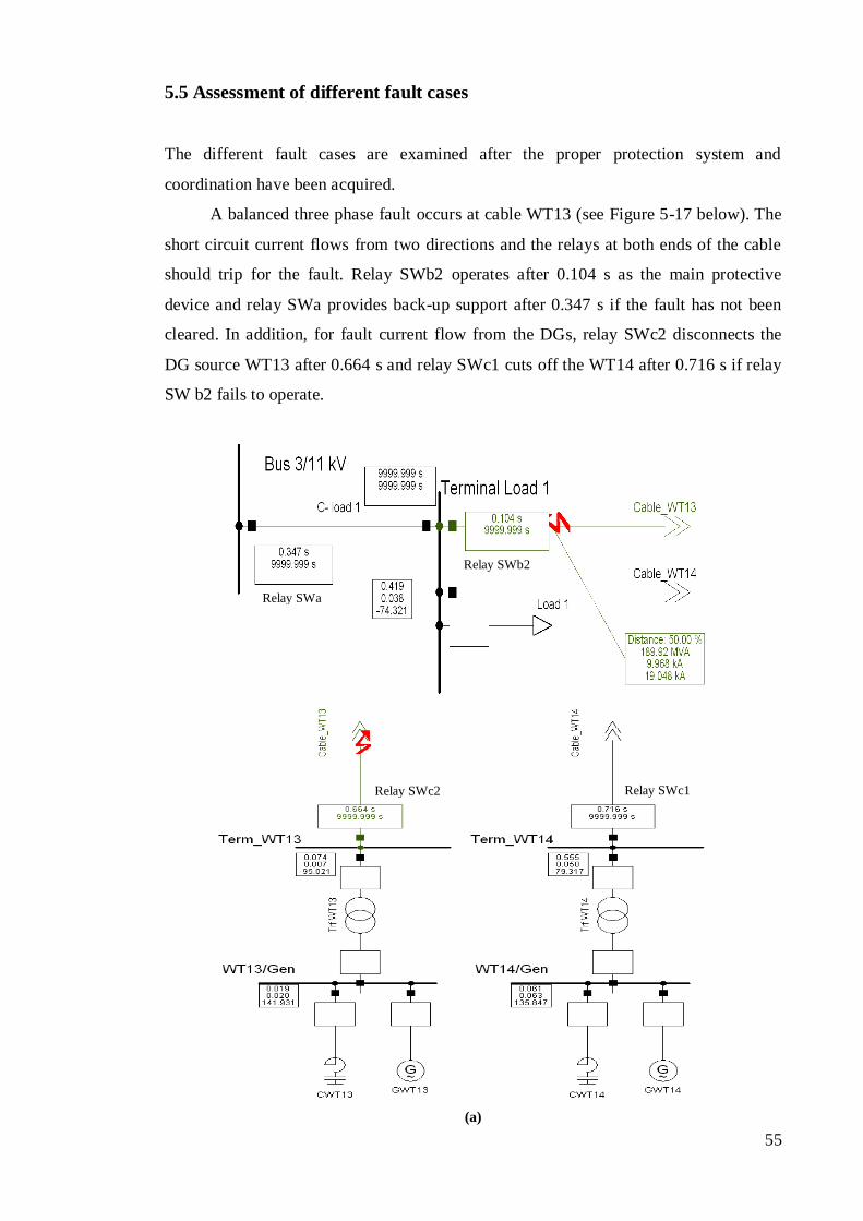
55

5.5 Assessment of different fault cases

The different fault cases are examined after the proper protection system and

coordination have been acquired.

A balanced three phase fault occurs at cable WT13 (see Figure 5-17 below). The

short circuit current flows from two directions and the relays at both ends of the cable

should trip for the fault. Relay SWb2 operates after 0.104 s as the main protective

device and relay SWa provides back-up support after 0.347 s if the fault has not been

cleared. In addition, for fault current flow from the DGs, relay SWc2 disconnects the

DG source WT13 after 0.664 s and relay SWc1 cuts off the WT14 after 0.716 s if relay

SW b2 fails to operate.

(a)

Relay SWa

Relay SWb2

Relay SWc2 Relay SWc1

56

(b)

Figure 5-17 Three-phase fault at small wind farm, showing

(a) the relay tripping time and in

(b) time overcurrent plot displays the characteristics

In the second case, when a single phase to the earth fault occurs at cable C-LW2

of one of the collection transformers, directional OC earth relay LW1a trips this fault

after 0.245 s and the directional OC relay A operates as back-up device after 0.85 s. For

this reason the earth fault occurs at the LV side of the transformer and is unable to cause

zero sequence current flowing in the HV side. The phase element of relay A will

provide support because the earth element of relay A will not sense the fault. From

Figure 5-18, the singe phase to the ground fault also causes the phase element of relay

LW1a to trip after 0.27s. However, both the earth element and the phase element of the

relay will trip the same circuit breaker and act independently. As long as they satisfy the

requirement for selectivity, the correct coordination or tripping sequence can be

guaranteed.

Relay C

Relay SW a

Relay SW b2

57

Figure 5-18 Single phase fault at the large wind farm

5.6 Chapter summary

The protection schemes for the network in two situations (with or without DGs) have

been successfully achieved and the problems related to DGs have been solved through

the readjustment on the relay parameters, the install of new directional relays, the

replacement of new characteristics on the relays. Both of them were simulated in the

DIgSILENT software, which includes the network modeling, fault current analysis, time

overcurrent plot display, and the operation of protective devices in case of a fault. The

protection system without DGs connection is compromised with overcurrent relays and

fuses, and the protection coordination is the coordination between overcurrent devices.

However, after the proliferation of DGs, the original protective devices need to be

adjusted and new protective devices must be added into the system. The proper

protection coordination requires reconsideration.

Relay A

Relay LW1a

Relay LW1b Relay LW2b

60

Figure 5-19 Relay parameters for the main network

62

Figure 5-20 Relay parameters for the large wind farm

64

Figure 5-21 Relay parameters for the small wind farm

65

6. Meshed networks simulated in DIgSILENT


In the radial MV network, overcurrent relays are employed to achieve protection

coordination. In the distribution networks with multiple sources, time-graded

overcurrent relays with directional sensing units are used to achieve proper coordination

in the protection scheme. However, in line with increased interest in the improvement of

the quality of electricity distribution, meshed network, including closed-loop feeder

operations, is becoming a subject of great interest and recognized to have the great

potential [29].

Protection coordination has become even more complicated as the result of using the

meshed mode. For such meshed networks with multiple sources, it is hard to satisfy the

coordination requirements and the calculation process is complicated when using OC

protection. Compared with the OC protection scheme, the distance protection scheme

employed in protecting the meshed network is simpler and the coordination between

relays is relatively easier to acquire. The distance-based protection schemes that protect

the typical meshed distribution networks are demonstrated in this chapter.

6.2 Network modeling

A typical section of the distribution network is adopted from [30]. The network

comprises a 33 kV, 11Hz external grid and supplies the 11 kV busbar through two

parallel 33/11 kV/kV transformers. The total of the loads, 4.85 MW, are constant

impedance static loads distributed along the feeder. A detailed description and

parameters regarding the network are given in Appendix 3.

The general philosophy to design the protection system of a network is to divide the

system into separate zones that can be individually protected and disconnected on the

occurrence of a fault [3]. Each relay in a protection system has the responsibility to trip

a predefined circuit breaker (CB) when the fault occurs in its required zones.

66

Bus 1

33 kV

Bus 2

11 kVBus 3

11 kV

Bus 4

11 kV

Bus 5

11 kV

Relay 1

I>

51

T 33/11 20MVA

External grid

3500 MVA

Bus 6

11 kV

Bus 7

11 kV

Cable 1

Cable 2 Cable 3 Cable 4

Cable 5

Cable 6

Relay 5

I>

51

Relay 2a

Z>

21

Relay 2b

Z>

21

Relay 3a

Z>

21

Relay 3b

Z>

21

Relay 4a

Z>

21

Relay 4b

Z>

21

Relay 6b

Z>

21

Relay 6a

Z>

21

Load 1

Load 2

Load 3

Load 4

33 kV overhead line

T 33/11 20MVA

33 kV overhead line

Figure 6-1 Singe line diagram of the meshed distribution network

6.3 Meshed network without DGs

6.3.1 The selection and settings of protective devices

The protection system designed for the meshed network can be divided into two parts.

One part is the OC protection and overcurrent relays are installed to protect cable 1 and

cable 5 from the short circuit events (Figure 6-1). Relay 1 and relay 5 are OC relays and

both follow extremely inverse (EI) characteristics. The other part is the close loop

protection, which is mainly comprised of feeders see currents flow from more than one

direction (relays 2a, 2b, 3a, 3b, 4a, 4b, 6a, 6b). Distance relays are installed at both ends

of every busbar with a directional sensing unit around the loop circuit. All distance

relays adopted in the protection system follow the MHO characteristic. They are GE

distance type. The GE distance relay type is selected from the DIgSILENT global

library and needs to be set in each protection zone separately. The settings for distance

relays have been explained in the previous Section 2.4.

The R-X plot represents the characteristic of a distance relay. The impedance of the

connected lines and transformers in the network displayed also in the plot, allows us to

clearly observe the reaching zone of each distance relay. The R-X plot can provide users

with short circuit or load flow calculations as well. The following information can be

read from it [25]: the name of the relay, measured impedances seen from the relay

location, the fault type, the actual tripping time of the relay and which zone is tripped.

67

Figure 6-2 The R-X plots display a 2-phase fault

The information is essential when assessing the relay operation of the faults at the end

of the zone in order to guarantee the sensitivity. For instance, as shown in Figure 6-2, if

a 3-phase fault occurs at the zone 3 of the distance relay dis2a, the improper settings

result in the relay dis2a not sensing the fault current. The circle should be set larger to

include the fault. After the relay settings have been edited manually, the relay dis2 trips

correctly when the same fault occurs (0.67 s). The information can be read from the R-X

plot: the name is relay dis2a; the fault type is a 3-phase fault; the tripping time for this

fault is 0.67 s; the fault location is within zone 3. Thus, the fault location can be

distinguished directly and the correct reach of the zone can be adjusted.

It is common to set the relay characteristic angle a little smaller than the line angle in

order to accept a small amount of fault resistance without producing under-reach

(Section 2.4.3). Therefore, in this protection system, the characteristic angles of distance

relays are set at 30o, which is a little greater than the line impedance angle that is 29

o.

The directional distance relays are set to operate for faults occurring at the forward

direction. However, when a 3-phase fault occurs at the busbar, the MHO relay locates in

the feeder may become non-directional and trip the reverse busbar fault since the

voltage at the busbar decreases to zero. A way to prevent this incorrect reverse

operation is to authorize the voltage memory unit of the MHO distance relay to accept

the polarizing voltage signal. This enables high speed MHO protection to operate

Zone 1

Zone 2

Zone 3

Zone 1

Zone 2

Zone 3 Fault

location Fault

location

The line

impedance The line

impedance

68

correctly on the close-in faults, provided that the protected circuit is energized before

the short circuit is applied [4].


The protection coordination should be examined in two parts. One part is the

coordination between the distance relays at the loop circuit, which is relatively simple.

The traditional criterion for loop feeder coordination was explained in Chapter 3. Firstly,

look around the loop, clockwise, relay dis 6b - relay dis 4b - relay dis 3b - relay dis 1b.

Then begin with relay dis 2a on the reverse direction around the loop this time.

Secondly, the appropriate settings are calculated based on the rules in Section 3.2 and

need to be examined in the time-distance plot to ensure correct protection coordination.

Figure 6-3 (a) displays the tripping time for the distance relays around counter

clockwise; the red curve represents the relay dis 6b and the purple curve represents the

relay dis 4b. It is clear to see that the zone 2 of the red curve is covered with a portion of

the zone 2 of the purple curve. This means that for faults occurring at the overlapping

zone, two relays will operate at the same time. Consequently, the coordination is lost

and a readjustment should be considered. In Figure 6-3 (b), there ARE no longer exists

the overlapping zones of distance relays after the resetting.

Another part is the coordination between distance relays locate at the loop feeder and

overcurrent relays locate outside the loop. It can be clearly seen that the loop is not

completely independent. The settings of some distance relays are also dependent on

their downstream OC relays or upstream OC relays. There are two significant formulas

mentioned in Section 3.2.1 that should be considered. For example, for the first rule and

Equation 3-2, the zone 2 of relay dis 4a is set to cover all the protected line, plus 25% of

the second longest line (cable 5) as illustrated before. Therefore, zone 2 of relay dis 4a

should be set as the back up protection when a fault occurs within 25% of cable 5 and it

only operates when the main protective relay 5 fails to operate. The operating time for

zone 2 is usually in the range of 0.3 to 0.6 s. For this network, the operating time for

zone 2 is 0.3 s, zone 3 is 0.65 s. Figure 6-4 shows an example; if a fault occurs at the

main protective zone of relay 5 (between bus 6 and bus 7), it will operate faster than

zone 2 and zone 3 of the distance relay (blue curve). This diagram is a time distance (T-

69

D) plot formed by DIgSILENT, and more information regarding the T-D path can be

found in A.1.4.

(a)

(b)

Figure 6-3 Example for overlapping of distance relays

The zone 2

of Relay 6b

The zone 2

of Relay 4b

The overlapping

zone

Relay 6b Relay 4b Relay 3b

70

Figure 6-4 Time-distance plot displays the distance relay working as a back-up

Figure 6-5 Time-distance plot that displays the OC relay working as a back-up

Zone 1 (Relay dis 4a)



Relay 5 Coordination margin

Relay 1

Relay dis 1a Relay dis 3a Relay dis 4a

Bus 6 Bus 7

Bus 3 Bus 4 Bus 5 Bus 6

71

For the second criterion (Equation 3-3), the OC relay 1 operates as a back-up protection

when the fault occurs on adjacent feeders, so relay 1 must be coordinated with its

downstream distance relays (relays 1a, 6b). See Figure 6-5; enough coordinating margin

is successfully achieved by observing the time distance plot formed by DIgSILENT.

Relay 1 will correctly operate as back up protection slower than the main protection (the

distance relays) for its downstream faults located between bus 3 and bus 6.

6.3.3 Relay parameters and characteristics

Figure 6-6 shows the parameters of the relay dis 3a. This is the output of relay

parameters given by DIgSILENT. The type of the relay dis 3a is GE distance. The

current transformer ratio is 300A/5A and the voltage transformer ratio is 11000V/110V.

The settings of relay impedance of zone 1, zone 2 and zone 3 is 4 Ω, 6.7 Ω and 7 Ω. All

3 zones have the same characteristic angle (30o) and they both trip for the forward

direction. The tripping time of zone 2 is 0.3 s and the tripping time of zone 3 is 0.65 s.

All the parameters regarding the rest of distance relays can be read from Appendix 4.

Figure 6-6 The parameters of relay 3a

Figure 6-7 displays the characteristics in the R-X plot for distance relays installed

around clockwise in the loop circuit (relay 2a, relay 3a, relay 4a, relay 6a). Further

information about the relay settings can be found in Appendix 4.

72

Figure 6-7 Characteristics of distance relays in clockwise direction


The correct protection system for the meshed network is examined by the following

fault situation.

In Figure 6-8, a three-phase short circuit occurs at 90% of cable 3 and is cleared

by zone 2 of relay dis 3a after 0.32 s, and by relay dis 3b immediately. From the

tripping times displayed, relay dis 2a operates with a time delay if the relay dis 4a fails

to disconnect the circuit. The overcurrent relay 1 also sees the fault (0.96s). In the other

direction, zone 2 of relay dis 4b and zone 3 of relay dis 6b sense the fault and trip the

circuit breaker separately after 0.32 s, 0.67 s, respectively.

73

Figure 6-8 Three phase fault at 90% of cable 3

6.4 Meshed network with DGs connected

6.4.1 The network modeling and the protection system

The proper protection coordination has acquired in the meshed network. However, the

additional DGs connected to the network need to be reconsidered. Figure 6-9 shows the

two 5 MW wind farms are connected to the network through 11/0.69 kV/kV

transformers, and the power output of the wind farm is 79% of the rated power output

(3.9 MW). The wind farm is composed of ten paralleled standard induction generators

each rated at 500 kW.

Due to the penetration of DGs, new protective relays need to be added to the protection

system (Figure 6-9). Cable 1 now sees the fault currents flowing from multiple sources,

so the directional OC relays should be installed at both ends of the cable 1.

Consequently, relay 1a and relay 1b are adopted directional OC relays and they both

follow the IDMT characteristics. As for the rest of the protection system, the existing

relays can protect the network through proper adjustments. Relays 2a, 2b, 3a, 3b, 4a, 4b,

Relay dis 3a

Relay dis 3b

Relay dis 2a

Relay 1

Relay dis 4a

Relay dis 4b

Relay dis 6b Relay dis 6b

74

6a, and 6b are sill directional distance relays. Relay 5 sees the fault current flow from

one direction and the OC protection is capable of protecting the circuit.

Bus 1

33 kV

Bus 2

11 kVBus 3

11 kV

Bus 4

11 kV

Bus 5

11 kV

Relay 1a

Idir>

67

T 33/11 20MVA

External grid

3500 MVA

G

Bus 6

11 kV

Bus 7

11 kV

Cable 1

Cable 2 Cable 3 Cable 4

Cable 5

Cable 6

Relay 5

I>

51

Relay 2a

Z>

21

Relay 2b

Z>

21

Relay 3a

Z>

21

Relay 3b

Z>

21

Relay 4a

Z>

21

Relay 4b

Z>

21

Relay 6b

Z>

21

Relay 6a

Z>

21

Load 1

Load 2

Load 3

Load 4

T 11/0.69 20MVA

33 kV overhead line

G

T 11/0.69 20MVA

T 33/11 20MVA

33 kV overhead line

Relay 1b

Idir>

67

Figure 6-9 Singe line diagram of the meshed distribution network with DGs


The distance relays have the advantages such as fixed reach, and inherent directionality

so that the distance-based protection can ensure the coordination easier than the OC

protection in the meshed network. Nevertheless, the addition of distributed generators

into the distribution network will produce raised impacts on the protection coordination.

In terms of distance protection, as stated in Section 4.4, the current flowing from the

DGs may result in the unwanted under reaching problem. Figure 6-10 demonstrates a 2-

phase short circuit that occurs at 50% of cable 3 and the fault location belongs to zone 2

of relay dis 2a. Without DGs connected, zone 2 of relay dis 2a could sense the fault and

make the correct response after 0.32 s. In the case of DGs connected, although relay dis

2a still senses the fault, the fault is beyond the circle of zone 2 and will be regarded as a

zone 3 fault and be cleared after 0.67 s. Predictably, the coordination is then lost and

readjustment is crucial to adapt to the penetration of the DGs.

75

Figure 6-10 Example for under reaching of a distance relay

76

The conventional method recognizes the DGs as an infeed source and calculates the

reaching of zone 2 and zone 3 with the infeed factor. Fortunately, when simulating the

network in DIgSILENT, the R-X and time distance plots are available. They have

provided effective outcomes to study the coordination of distance-based protection (as

described in Section 6.3.2). It is easier to verify the reaching zone of the distance relay

according to the R-X plot (Figure 6-10). The time distance plot gives the tripping time

of the distance relay and shows the protection coordination clearly. For example, Figure

6-11 shows that the proper coordination is acquired and the under reaching problem is

solved around the counter clockwise direction (relay 2a, relay 3a, relay 4a, relay 6a).

Figure 6-11 The time distance plot displays the relays in the clockwise direction


After the readjustments and replacements for relays in the meshed network with DGs,

the protection coordination has been achieved again. The different fault situations have

been tested.

In the first scenario, Figure 6-12 shows that a two phase fault at 20% of cable 1

near bus 2 will be cleared by main protective devices at both ends of the cable in 0.947 s

(relay 1a) and 0.09 s (relay 1b). Relay 2b and relay 6a will provide back-up protection

for relay 1b after 0.32 s and 0.67 s respectively.

77

Another SC situation at cable 4 in Figure 6-13 is a three balanced fault at 80% of

the cable. It will be cleared by the main protective relays 4a and 4b instantaneously.

Relay 3a (0.67 s), relay 2a (0.82 s) and relay 1a (1.095 s) will all sense the fault current

and provide back-up support for relay 4a. As for the other direction, zone 2 of relay 6b

breaks the circuit if relay 4b fails to trip the fault.

Figure 6-12 Two phase fault at cable 2

Relay 1a Relay 2b

Relay 6a

Relay 1b

78

Figure 6-13 Three phase fault at cable 4

6.5 Chapter summary

In this chapter, it was shown that the distance-based protection scheme is capable of

ensuring the protection coordination in the meshed networks. The protection

coordination must be studied from two aspects; one is the coordination between

distance relays and this can be acquired through appropriate settings (the R-X plot), and

clearly displayed in the time distance plot; another aspect is the consideration on the

distance and overcurrent relays, their coordination is studied with the help of time

distance plot (including the tripping time of the overcurrent and distance relays). The

under reaching is the influence caused by DGs and is clearly an issue, however, it can

be eliminated to regain the coordination through readjustment.

Relay 1a

Relay 2a

Relay 6b Relay 6a

Relay 3a Relay 4a

Relay 4b

Relay 2b Relay 3b

79

7. Conclusion

In this chapter, an overview of the project is now provided, key points are summarized

and the major conclusions are drawn. Furthermore, some of the issues that have not

been elaborated are now discussed and recommendations for future work in the

protection coordination related to DGs are provided.

7.1 Project summary

The first goal of this research was to define and describe the major steps in the

protection coordination of a power network. The key challenges in this process have

been pointed out. If the protection coordination has not been done properly, the

protection would not protect the network appropriately. For example, the unwanted

protective devices could trip for a fault occurring; the protective devices could not sense

a fault and result in the damage on the network and interrunption in the power supply.

The protection coordination has been investigatied using two typical test networks: a) a

MV radial distribution network and b) a meshed distribution network. It has been

concluded that the radial network can be protected by overcurrent (OC) protection and

the protection coordination between OC relays has been successfully demonstrated (see

Section 5.3). In this research the DIgSILENT software package has been applied and

scrutinized from its applicability for the protection coordination. It has been concluded

that the DIgSILENT software package can be successfully used for both the network

modeling and protection coordination. The time overcurrent plot provided by

DIgSILENT was a key tool to study the protection coordination between OC relays in

the radial network. Another network analysed was a meshed distribution network. In

this case the protection coordination has been determined by the network topology (see

Section 6.3). Since the meshed network means that even the network is supplied by only

one source, some of the network feeders may see currents coming from two different

directions. Protection of such a meshed network was not possible by using the pure OC

protection. It has been demonstrated how the distance-based protection can efficiently

protect meshed networks and reach an optimal protection coordination. Here the

attention must be paid on avoiding the overlapping zone of distance relays. The

DIgSILENT software package has provided the R-X plot and the time distance plot to

assist studying the protection coordination between different distance relays.

80

The second goal of this research was to explore the impacts caused by DGs on

protection coordination. Using the DIgSILENT software package, the DGs were

modelled and integrated in the abovementioned networks (radial and meshed). It has

been concluded that the protection coordination was influenced because the fault current

magnitudes and the fault current directions have been changed after introducing DGs in

the networks. It has been concluded and demonstrated that in networks with DGs, the

protection concepts must be based on the multiple supply sources for the grid. Therefore,

the directional OC relays were introduced to protect the networks with DGs and DGs

itself. The investigation of the protection coordination of the MV network with DGs

revealed three main problems and dealt with their solutions (see Section 4.2-4.4, Section

5.4). These main problems were:

1. The loss of grading margin between the protective relays, which can be

solved by readjusting the relay parameters with the help of the time overcurrent

plot.

2. The false tripping problem, which can occur at the OC relays located in

feeders with DGs connected. These OC relays were replaced by the directional

OC relays.

3. The blinding issue, which can occur at the OC relays located between the

fault point and the relay. A combination of IDMT and definite-time

characteristics OC relays were used to solve this difficulty.

The discussion of the protection coordination in the meshed distribution network with

DGs connected in Section 6.4 highlighted the DGs influence on the distance relays’

settings. After the integration of DGs, the protection system was still designed as the

distance-based protection. However, the coordination was lost because the DG could

have an impact (e.g. the infeed current) on distance relays and cause under-reach issue.

Therefore, the relay settings must be changed to adapt the extra fault current sources in

order to regain the protection coordination. Attention should be also paid on the time

distance plot provided by DIgSILENT, which assists the process of the protection

coordination not only between distance relays, but also between distance relays and an

OC relays.

The test networks used in the project were successfully simulated using the DIgSILENT

software package. There were differences in the relay tripping time and the grading

81

margin in situations with or without DGs provided by the examples simulated in

DIgSILENT. In terms of each relay characteristic, they played a vital role in the

coordination methods in this project. As a means to display the characteristic curves and

to give us a clear understanding of coordination, the time-overcurrent plot, the R-X plot

and the time-distance plot were provided by DIgSILENT. To proper design the

protection system and acquire protection coordination, it was possible to select the

proper protective devices from DIgSILENT, to set feasible parameters and do the

proper coordination procedures with the help of DIgSILENT.

7.2 Future work

The DIgSILENT library has not provided suitable types of distance relays for earth

faults protection so the obvious extension of this work would be to repeat the

coordination process for the earth faults protection in the meshed distribution network.

As far as the problems caused by DGs concerned, the readjustment of the relay settings

or additional relays installed can make the protection system work properly. However,

relays can not respond to the fault correctly if the DGs are disconnected. For example, if

the settings of distance relays are based on DGs, the distance relays may over-reach if

the DGs are disconnected. Therefore, a more advanced adaptive protection scheme that

can automatically make adjustments for different power system conditions will be

inevitable.

82

8. References

[1] M. H. Hairi, K. Alias, Aras, Mohd Shahrieel bin Mohd, M. F. M Basar, S. P Fah,

2010, “Inverse definite minimum time overcurrent relay coordination using

computer aided protection engineering”, in Power Engineering and Optimization

Conference (PEOCO), 2010 4th International, 23-24 June 2010, 304 - 307

[2] J. M. Gers, E. J Holmes, 2004, Protection of electricity distribution networks,

London: Institution of Electrical Engineers, 2004 , page3-5

[3] F. Coffele, 2012, Adaptive protection solution for future active power distribution

networks, Dissertation Project, PHD Electrical and Electronic Engineering,

University of Strathclyde

[4] AREVA T&D, 2002, Network protection and automation guide—protective

relays, measurement & control

[5] P. Bancroft, 2011, Protection Coordination of a Typical Round 2 Off Shore Wind

Farm Grid Connection, Dissertation Project, MSc Electrical Power Systems

Engineering, University of Manchester

[6] J. L. Blackburn, T. J. Dmin, 1998, Protective Relaying—Principles and

applications, New York: Narcek Dejjer, Inc.

[7] [https://www.gedigitalenergy.com/smartgrid/Mar07/article7.pdf]

[8] E. P. Sutherland, 1997, “Protective device coordination in an industrial power

system with multiple sources”, in Industry Applications, IEEE Transactions on

Jul/Aug 1997, 33 , Issue: 4, pp: 1096 - 1103

[9] T. Mashau, S. Kibaara, S. Chowdhury, S. P. Chowdhury, 2011, “Impact of

distributed generation on protection coordination in a radial distribution feeder”,

Universities' Power Engineering Conference (UPEC), Proceedings of 2011 46th

International, 5-8 Sept. 2011, pp: 1 - 5

[10] I.M Chilvers, N. Jenkins, P. A. Crossley, 2004, “The use of 11 kV distance

protection to increase generation connected to the distribution network”, Eighth

IEE International Conference on Developments in Power System Protection,

Page(s): 551 - 554 Vol.2

[11] I.M Chilvers, N. Jenkins, P. A. Crossley, 2005, “Distance relaying of 11 kV

circuits to increase the installed capacity of distributed generation”, IEE

Proceedings-Generation, Transmission and Distribution, Vol. 152, pp. 40 – 46,

2005.

http://ieeexplore.ieee.org/search/searchresult.jsp?searchWithin=p_Authors:.QT.Hairi,%20M.%20H..QT.&searchWithin=p_Author_Ids:37546893900&newsearch=true

http://ieeexplore.ieee.org/search/searchresult.jsp?searchWithin=p_Authors:.QT.Alias,%20K..QT.&searchWithin=p_Author_Ids:37546898700&newsearch=true

http://ieeexplore.ieee.org/search/searchresult.jsp?searchWithin=p_Authors:.QT.Aras,%20Mohd%20Shahrieel%20bin%20Mohd.QT.&searchWithin=p_Author_Ids:37394924700&newsearch=true

http://ieeexplore.ieee.org/search/searchresult.jsp?searchWithin=p_Authors:.QT.Basar,%20M.F.M..QT.&newsearch=true

http://ieeexplore.ieee.org/xpl/mostRecentIssue.jsp?punumber=5538456


http://ieeexplore.ieee.org/search/searchresult.jsp?searchWithin=p_Authors:.QT.Mashau,%20T..QT.&newsearch=true

http://ieeexplore.ieee.org/search/searchresult.jsp?searchWithin=p_Authors:.QT.Kibaara,%20S..QT.&newsearch=true

http://ieeexplore.ieee.org/search/searchresult.jsp?searchWithin=p_Authors:.QT.Chowdhury,%20S..QT.&newsearch=true

http://ieeexplore.ieee.org/search/searchresult.jsp?searchWithin=p_Authors:.QT.Chowdhury,%20S.%20P..QT.&newsearch=true



http://ieeexplore.ieee.org/search/searchresult.jsp?searchWithin=p_Authors:.QT.Chilvers,%20I.M..QT.&searchWithin=p_Author_Ids:37266648200&newsearch=true

http://ieeexplore.ieee.org/search/searchresult.jsp?searchWithin=p_Authors:.QT.Jenkins,%20N..QT.&searchWithin=p_Author_Ids:37272578700&newsearch=true

http://ieeexplore.ieee.org/search/searchresult.jsp?searchWithin=p_Authors:.QT.Crossley,%20P.A..QT.&searchWithin=p_Author_Ids:37276371800&newsearch=true

http://ieeexplore.ieee.org/xpl/articleDetails.jsp?tp=&arnumber=1364937&contentType=Conference+Publications&searchField%3DSearch_All%26queryText%3Dthe+use+of+11+KV+distance+protection





83

[12] D. Martin, P. Sharma, 2012, “Distance protection in distribution systems: How it

assists with integrating distributed resources”, 2012 65th Annual Conference for

Protective Relay Engineers, pp. 166-167

[13] V. P. Mahadanaarachchi, R. Ramakuma, 2008, “Impact of distributed generation

on distance protection performance - A review”, Power and Energy Society

General Meeting - Conversion and Delivery of Electrical Energy in the 21st

Century, 2008 IEEE, pp. 1-7.

[14] Kalam, D. P. Kothari, 2010, Power system protection and communication, New

age science limited

[15] D. Uthitsunthorn, T. Kulworawanichpong, 2010, “Distance protection of a

renewable energy plant in electric power distribution systems”, 2010

International Conference on Power System Technology, pp. 1-6.

[16] J. Sadeh, V. Amintojjar, M. Bashir, 2011, “Coordination of overcurrent and

distance relays using hybrid Particle Swarm Optimization”. 2011 International

Conference on Advanced Power System Automation and Protection (APAP), Vol.

2, pp. 1130 – 1134.

[17] J. A. Artinez, J. Martin-Arnedo, 2009, “Impact of distributed generation on

distribution protection and power quality”, in Power & Energy Society General

Meeting, IEEE, 26-30 July 2009, 1-6.

[18] K. Vijeta, D. V S S Siva Sarma, 2012, “Protection of distributed generation

connected distribution system”, Advances in Power Conversion and Energy

Technologies (APCET), 2012 International Conference, pp: 1 - 6

[19] F. A. Viawan, D. Karlsson, A. Sannino, J. E. Daalder, 2006, “Protection scheme

for meshed distribution systems with high penetration of distributed generation”,

Power Systems Conference: Advanced Metering, Protection, Control,

Communication, and Distributed Resources, pp: 99 - 104

[20] Girgis, A. Adly, 2001, “Effect of distributed generation on protective device

coordination in distribution system”, in Power Engineering Conference, 115 -

119

[21] B. Hussain, S. M. Sharkh, & S. Hussain, 2010, “Impact studies of distributed

generation on power quality and protection setup of an existing distribution

network” , in 2010 International Symposium on Power Electronics, Electrical

Drives, Automation and Motion

http://ieeexplore.ieee.org/xpl/articleDetails.jsp?tp=&arnumber=6201231&contentType=Conference+Publications&searchField%3DSearch_All%26queryText%3Ddistance+protection+in+distribution+systems

http://ieeexplore.ieee.org/xpl/articleDetails.jsp?tp=&arnumber=6201231&contentType=Conference+Publications&searchField%3DSearch_All%26queryText%3Ddistance+protection+in+distribution+systems


http://ieeexplore.ieee.org/search/searchresult.jsp?searchWithin=p_Authors:.QT.Mahadanaarachchi,%20V.P..QT.&searchWithin=p_Author_Ids:38093856900&newsearch=true

http://ieeexplore.ieee.org/search/searchresult.jsp?searchWithin=p_Authors:.QT.Ramakuma,%20R..QT.&newsearch=true

http://ieeexplore.ieee.org/xpl/articleDetails.jsp?tp=&arnumber=4596707&contentType=Conference+Publications&searchField%3DSearch_All%26queryText%3Dimpact+of+distributed+generation+on+distance+protection+performance

http://ieeexplore.ieee.org/xpl/articleDetails.jsp?tp=&arnumber=4596707&contentType=Conference+Publications&searchField%3DSearch_All%26queryText%3Dimpact+of+distributed+generation+on+distance+protection+performance




http://ieeexplore.ieee.org/search/searchresult.jsp?searchWithin=p_Authors:.QT.Uthitsunthorn,%20D..QT.&newsearch=true

http://ieeexplore.ieee.org/search/searchresult.jsp?searchWithin=p_Authors:.QT.Kulworawanichpong,%20T..QT.&searchWithin=p_Author_Ids:37394155800&newsearch=true

http://ieeexplore.ieee.org/xpl/articleDetails.jsp?tp=&arnumber=5666058&contentType=Conference+Publications&searchField%3DSearch_All%26queryText%3Ddistance+protection+of+a+renewable+energy





http://ieeexplore.ieee.org/search/searchresult.jsp?searchWithin=p_Authors:.QT.Vijeta,%20K..QT.&searchWithin=p_Author_Ids:38485188100&newsearch=true

http://ieeexplore.ieee.org/search/searchresult.jsp?searchWithin=p_Authors:.QT.Girgis,%20Adly%20A..QT.&searchWithin=p_Author_Ids:37276185200&newsearch=true

84

[22] R. A. Walling, R. Saint, R. C. Dugan, J. Burke, A. Kojovic, 2008, “ Summary of

Distributed Resources Impact on Power Delivery Systems”, IEEE Transactions on

Power Delivery”, Vol.23, no.3, pp. 1636 - 1644

[23] J. A. Silva, H. B. Funmilayo, K. L. Butler-Purry, 2007, “Impact of distributed

generation on the IEEE 34 node radial test feeder with overcurrent protection”,

NAPS '07. 39th North American, pp. 49 - 57

[24] K. Kauhaniemi, L. Kumpulainen, 2004, “Impact of distributed generation on the

protection of distribution network”, Eighth IEE International Conference

on developments in Power System Protection, Vol.1, pp. 315 - 318

[25] DIgSILENT Power Factory, User’ manual

[26] J. Ma, J. Li, Z. Wang, 2010, “An adaptive distance protection scheme for

distribution system with distributed generation”, 5th International Conference on

Critical Infrastructure (CRIS), pp. 1-4

[27] G. Peltekis, 2011, Protection coordination of future networks with high wind

energy penetration, Dissertation Project, MSc Electrical Power Systems

Engineering, University of Manchester

[28] M. Brahma, Sukumar, A. A. Girgis, 2002, “Microprocessor-based reclosing to

coordinate fuse and recloser in a system with high penetration of distributed

generation”, Power Engineering Society Winter Meeting, IEEE , 453 - 458 vol.1

[29] F. A Viawan, D. Karlsson, 2007, “ Various protection schemes for closed loop

feeders with synchronous machine based distributed generation and their impacts

on reliability”, Power Tech, 2007 IEEE Lausanne, pp. 1170 - 1175

[30] I. M. Chilvers, 2005. "11kV Cable Protection to Permit Increase in Distributed

Generation," Ph.D thesis, Faculty of Engineering and Physical Sciences, University

of Manchester, Manchester

http://ieeexplore.ieee.org/search/searchresult.jsp?searchWithin=p_Authors:.QT.Silva,%20J.A..QT.&searchWithin=p_Author_Ids:37832183900&newsearch=true




http://ieeexplore.ieee.org/search/searchresult.jsp?searchWithin=p_Authors:.QT.Kauhaniemi,%20K..QT.&searchWithin=p_Author_Ids:37266546500&newsearch=true

http://ieeexplore.ieee.org/search/searchresult.jsp?searchWithin=p_Authors:.QT.Kauhaniemi,%20K..QT.&searchWithin=p_Author_Ids:37266546500&newsearch=true



http://ieeexplore.ieee.org/search/searchresult.jsp?searchWithin=p_Authors:.QT.Jing%20Ma.QT.&searchWithin=p_Author_Ids:37311284400&newsearch=true

http://ieeexplore.ieee.org/search/searchresult.jsp?searchWithin=p_Authors:.QT.Jinlong%20Li.QT.&searchWithin=p_Author_Ids:37405667000&newsearch=true

http://ieeexplore.ieee.org/search/searchresult.jsp?searchWithin=p_Authors:.QT.Zengping%20Wang.QT.&searchWithin=p_Author_Ids:37279248600&newsearch=true

http://ieeexplore.ieee.org/xpl/articleDetails.jsp?tp=&arnumber=5617480&contentType=Conference+Publications&searchField%3DSearch_All%26queryText%3DAn+adaptive+distance+protection+scheme+for+distribution+sytsem

http://ieeexplore.ieee.org/xpl/articleDetails.jsp?tp=&arnumber=5617480&contentType=Conference+Publications&searchField%3DSearch_All%26queryText%3DAn+adaptive+distance+protection+scheme+for+distribution+sytsem


http://ieeexplore.ieee.org/search/searchresult.jsp?searchWithin=p_Authors:.QT.Brahma,%20Sukumar%20M..QT.&searchWithin=p_Author_Ids:38476920700&newsearch=true

http://ieeexplore.ieee.org/search/searchresult.jsp?searchWithin=p_Authors:.QT.Girgis,%20Adly%20A..QT.&searchWithin=p_Author_Ids:37276185200&newsearch=true



85

9. Appendices

Appendix 1: DIgSILENT PowerFactory

A.1.1 Introduction

The calculation program PowerFactory, as written by DIgSILENT, is a computer aided

engineering tool for the analysis of transmission, distribution, and industrial electrical

power systems. It has been designed as an advanced integrated and interactive software

package dedicated to electrical power system and control analysis in order to achieve

the main objectives of planning and operation optimization [25].

The name DIgSILENT stands for "DIgital SImuLation and Electrical NeTwork calcula-

tion program''. It had been used in this dissertation for simulating the networks and

analyzing protection schemes. In order to give a general DIgSILENT overview, some of

its functions used are explained in this section. More information referring to the

software can be found in the software User’s Mannual.

A.1.2 Short-Circuit Analysis

The short-circuit calculation in PowerFactory is able to simulate various kinds of faults

using different representations and calculation methods. The following fault types are

available: 3-Phase Short-Circuit, Single Phase to Ground, 3-Phase Short-Circuit

(unbalanced), etc. Examples of these methods include the IEC 60909/VDE 0102

method, the ANSI method and the IEC 61363 method. As opposed to the calculation

methods according to IEC/VDE and ANSI, which represent short-circuit currents by

approximations, the complete method evaluates currents without using approximations.

When it comes to accurate calculation of the currents after the onset of the fault, like in

this project, the complete method is more appropriate.

An example of the short-circuit command dialogue is shown in Figure 9-1, which is

used to define the general settings of the short-circuit calculation. In this case, the

‘complete’ method is employed to calculate the 3-phase short circuit fault. There are

more options accessible in the short-circuit calculation indicated by the dialogue. One

86

can manually edit the fault impedance for different purposes. Furthermore, the fault

location is also available that allows setting the relative distance of the line. This is

crucial when it relates to the reach zone of a distance relay.

Figure 9-1 Short circuit with the 'Complete' method

A.1.2 Protection Analysis

The PowerFactory protective devices are all stored in the cubicle connected to the

busbar and branch element, with CTs, VTs, circuit breaker and relays. Protective

devices include fuses that could operate on a switch stored in the same cubicle without

additional settings. Editing or adding new protective devices in the cubicle can be done

through right-clicking on a switch-symbol in the single line diagram. Selecting the

option to create a new protection device brings up a list with the following options [25]:

• Relay Model (ElmRelay)

• Fuse (RelFuse)

• Current Transformer (StaCt)

• Voltage Transformer (StaVt)

87

Figure 9-2 Relay model dialogue with selected type

Each of these options opens a dialogue to specify the device that is to be created. Newly

created devices are stored in the cubicle that was selected [25]. For instance, Figure 9-2

demonstrates a relay model that is equipment with a directional relay with the

combination characteristic of IDMT and definite time type (Rel-Ioc-Toc-Dirext). If the

current and voltage transformers have been created before the creation of the relay type,

they would be filling the slot automatically. If not, new VT and CT need to be defined

as the correct slot element.

A.1.3 Time-overcurrent plot

The time-overcurrent plot shows [25]:

• The time-overcurrent characteristics of relays

• The damage curves of transformers or lines

• Motor starting curves

• The currents calculated by a short-circuit or load-flow analysis and the resulting

tripping times of the relays

The time-overcurrent plot shows the results of short-circuit or load-flow analysis that

could help setting the relay tripping time and pick-up current. Because the currents

88

differ for each particular relay, a current line is drawn for each relay. The intersection of

the calculated current with the time-overcurrent characteristic is labeled with the

tripping time.

A 'grading margin' line, which shows the difference between the tripping times, may be

added by right-clicking the plot and selecting "Show Grading Margins''. The specific

procedures of editing different curves can be accessed in DIgSILENT. The grading

margins are shown as two lines in the diagram in DIgSILENT, plus and minus the

grading margin above and below the dragged tripping characteristic.

A.1.4 Time-Distance diagram

The coordination between OC relays is fulfilled with the help of time-overcurrent plot,

while the coordination between distance relays or distance relays and OC relays could

be checked based upon the time-distance diagram. Similar with time-overcurrent plots,

there are several methods to calculate the tripping time in time-distance diagrams. In

this dissertation, the Short-Circuit Sweep Method was selected for the most accurate

calculation. The diagram can be created only in the situation when a path has been

defined before. In the user’s manual, information on path definition is available. Figure

9-4 is an example of launching this function.

Figure 9-3 Short circuit sweep method

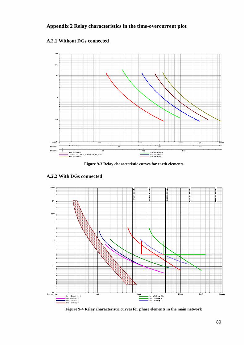
89

Appendix 2 Relay characteristics in the time-overcurrent plot

A.2.1 Without DGs connected

Figure 9-3 Relay characteristic curves for earth elements

A.2.2 With DGs connected

Figure 9-4 Relay characteristic curves for phase elements in the main network

90

Figure 9-5 Relay characteristic curves for earth elements in the main network

Figure 9-6 Relay characteristic curves for phase elements in the large wind farm

91

Figure 9-7 Relay characteristic curves for earth elements in the large wind farm

Figure 9-8 Relay characteristic curves for phase elements in the small wind farm

92

Figure 9-9 Relay characteristic curves for earth elements in the small wind farm

Appendix 3 Network data for meshed distribution network data

A.2.1 Induction generator parameters

Component Description Value

Nominal voltage (kV) 690

Rated output (kW) 500

Nominal factor (pu)

0.92

Stator Resistance (pu) 0.02803771

Stator Reactance (pu) 0.01

Rotor Leakage Reactance (pu) 0.01

Mag Reactance (pu) 4.236279

Pole pair 1

Table 9-1 Induction generator parameters

A.2.2 Line data

The 5 km, 33 kV overhead line was aluminum core steel reinforced (ACSR) cable, with

a cross sectional area of 150 mm2. The phase impedance data is:

93

ZOH = 0.1089 + j0.33759 Ω/km (9-1)

The 11 kV line consisted of 2 km of underground cables, which were based on a 3-core,

185 mm2 diameter aluminum conductors. The impedance data is:

ZUG = 0.165 + j0.094 Ω/km (9-2)

A.2.3 Transformer data and load data

The transformer parameters for the network are given in Table 9-2

Component description Value

Base (MVA) 20

Voltage ration (kV) 33/11

R (pu) 0.005

X (pu) 0.06

Vector group Dyn11

Component description Value

Base (MVA) 6

Voltage ration (kV) 11/0.69

R (pu) 0.01

X (pu) 0.05

Vector group Dyn11

Table 9-2 Transformer data

The loads in the network are modelled as stated in Table 9-3

Load Static load

Real power, P (MW) Reactive power, Q

(MVar)

1 0.30 0.0

2 0.20 0.0

3 0.35 0.0

4 0.40 0.6

Table 9-3 Load data

94

Appendix 4 Relay parameters for the meshed network

96

Figure 9-10 Relay parameters without DGs

100

Figure 9-11 Relay parameters with DGs

protection coordination in networks with renewable energy

Documents