protein adsorption kinetics under an applied

PROTEIN ADSORPTION KINETICS UNDER AN APPLIED ELECTRIC FIELD: AN OPTICAL WAVEGUIDE LIGHTMODE SPECTROSCOPY STUDY

by

MICHELLE A. BRUSATORI

DISSERTATION

Submitted to the Graduate School

of Wayne State University,

Detroit, Michigan

in partial fulfillment of the requirements

for the degree of

DOCTOR OF PHILOSOPHY

2001

MAJOR: CHEMICAL ENGINEERING Approved by: _______________________________ Advisor Date _______________________________ _______________________________ _______________________________

© COPYRIGHT BY


2001

All Rights Reserved

ii

Dedication

To my parents, Louis and Patricia Brusatori, for their love and

encouragement.

iii

Acknowledgements

I would like to acknowledge my advisor, Prof. Paul Van Tassel, for his

guidance and support and Dr. Joseph Smolinski for his assistance in the

development of experimental equipment.

iv

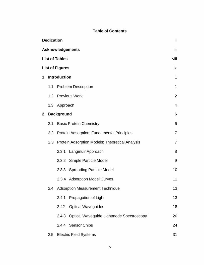
Table of Contents

Dedication ii

Acknowledgements iii

List of Tables viii

List of Figures ix

1. Introduction 1

1.1 Problem Description 1

1.2 Previous Work 2

1.3 Approach 4

2. Background 6

2.1 Basic Protein Chemistry 6

2.2 Protein Adsorption: Fundamental Principles 7

2.3 Protein Adsorption Models: Theoretical Analysis 7

2.3.1 Langmuir Approach 8

2.3.2 Simple Particle Model 9

2.3.3 Spreading Particle Model 10

2.3.4 Adsorption Model Curves 11

2.4 Adsorption Measurement Technique 13

2.4.1 Propagation of Light 13

2.42 Opitcal Waveguides 18

2.4.3 Optical Waveguide Lightmode Spectroscopy 20

2.4.4 Sensor Chips 24

2.5 Electric Field Systems 31

v

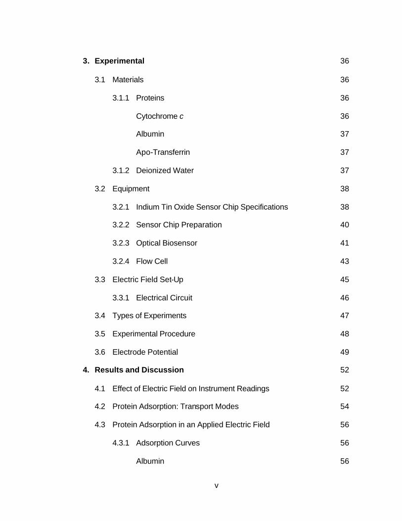
3. Experimental 36

3.1 Materials 36

3.1.1 Proteins 36

Cytochrome c 36

Albumin 37

Apo-Transferrin 37

3.1.2 Deionized Water 37

3.2 Equipment 38

3.2.1 Indium Tin Oxide Sensor Chip Specifications 38

3.2.2 Sensor Chip Preparation 40

3.2.3 Optical Biosensor 41

3.2.4 Flow Cell 43

3.3 Electric Field Set-Up 45

3.3.1 Electrical Circuit 46

3.4 Types of Experiments 47

3.5 Experimental Procedure 48

3.6 Electrode Potential 49

4. Results and Discussion 52

4.1 Effect of Electric Field on Instrument Readings 52

4.2 Protein Adsorption: Transport Modes 54

4.3 Protein Adsorption in an Applied Electric Field 56

4.3.1 Adsorption Curves 56

Albumin 56

vi

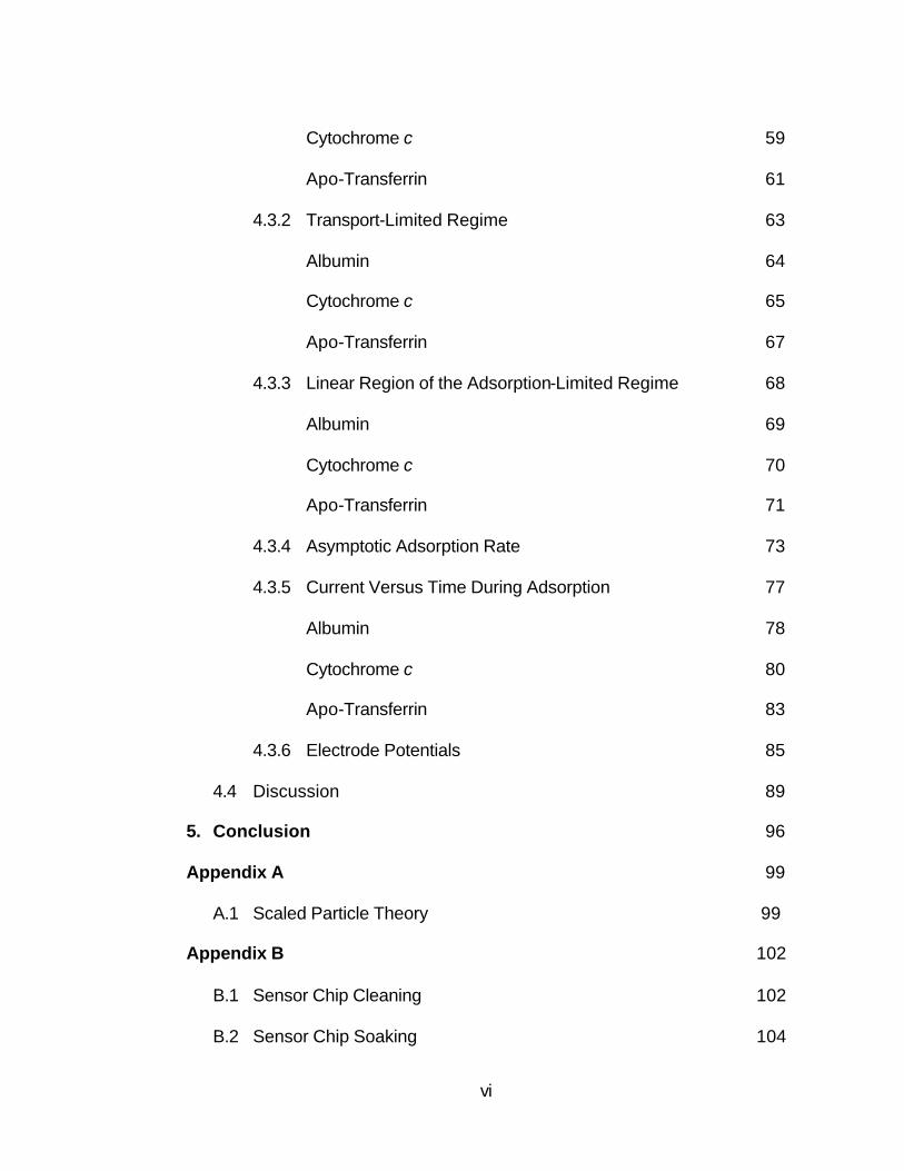
Cytochrome c 59

Apo-Transferrin 61

4.3.2 Transport-Limited Regime 63

Albumin 64

Cytochrome c 65

Apo-Transferrin 67

4.3.3 Linear Region of the Adsorption-Limited Regime 68

Albumin 69

Cytochrome c 70

Apo-Transferrin 71

4.3.4 Asymptotic Adsorption Rate 73

4.3.5 Current Versus Time During Adsorption 77

Albumin 78

Cytochrome c 80

Apo-Transferrin 83

4.3.6 Electrode Potentials 85

4.4 Discussion 89

5. Conclusion 96

Appendix A 99

A.1 Scaled Particle Theory 99

Appendix B 102

B.1 Sensor Chip Cleaning 102

B.2 Sensor Chip Soaking 104

vii

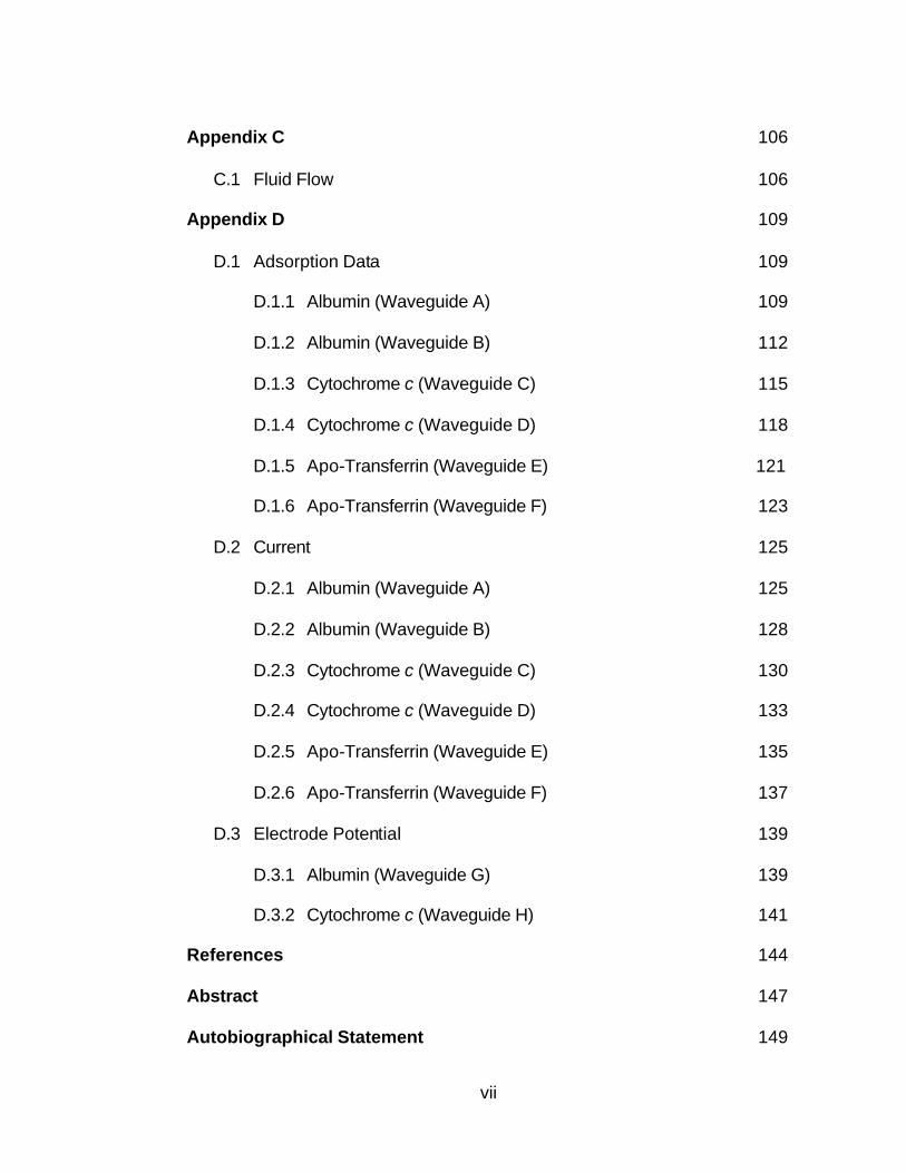
Appendix C 106

C.1 Fluid Flow 106

Appendix D 109

D.1 Adsorption Data 109

D.1.1 Albumin (Waveguide A) 109

D.1.2 Albumin (Waveguide B) 112

D.1.3 Cytochrome c (Waveguide C) 115

D.1.4 Cytochrome c (Waveguide D) 118

D.1.5 Apo-Transferrin (Waveguide E) 121

D.1.6 Apo-Transferrin (Waveguide F) 123

D.2 Current 125

D.2.1 Albumin (Waveguide A) 125

D.2.2 Albumin (Waveguide B) 128

D.2.3 Cytochrome c (Waveguide C) 130

D.2.4 Cytochrome c (Waveguide D) 133

D.2.5 Apo-Transferrin (Waveguide E) 135

D.2.6 Apo-Transferrin (Waveguide F) 137

D.3 Electrode Potential 139

D.3.1 Albumin (Waveguide G) 139

D.3.2 Cytochrome c (Waveguide H) 141

References 144

Abstract 147

Autobiographical Statement 149

viii

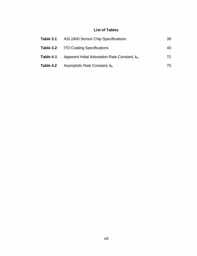
List of Tables

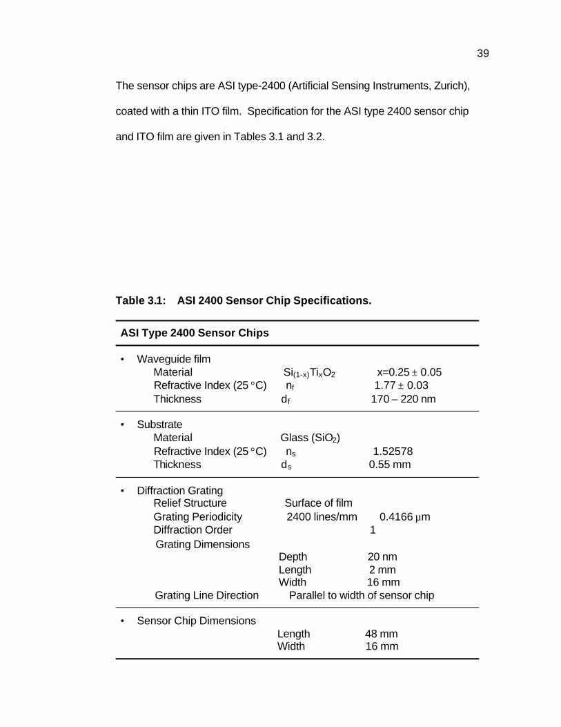
Table 3.1: ASI 2400 Sensor Chip Specifications 39

Table 3.2: ITO Coating Specifications 40

Table 4.1 Apparent Initial Adsorption Rate Constant, ka 72

Table 4.2 Asymptotic Rate Constant, kb 75

ix

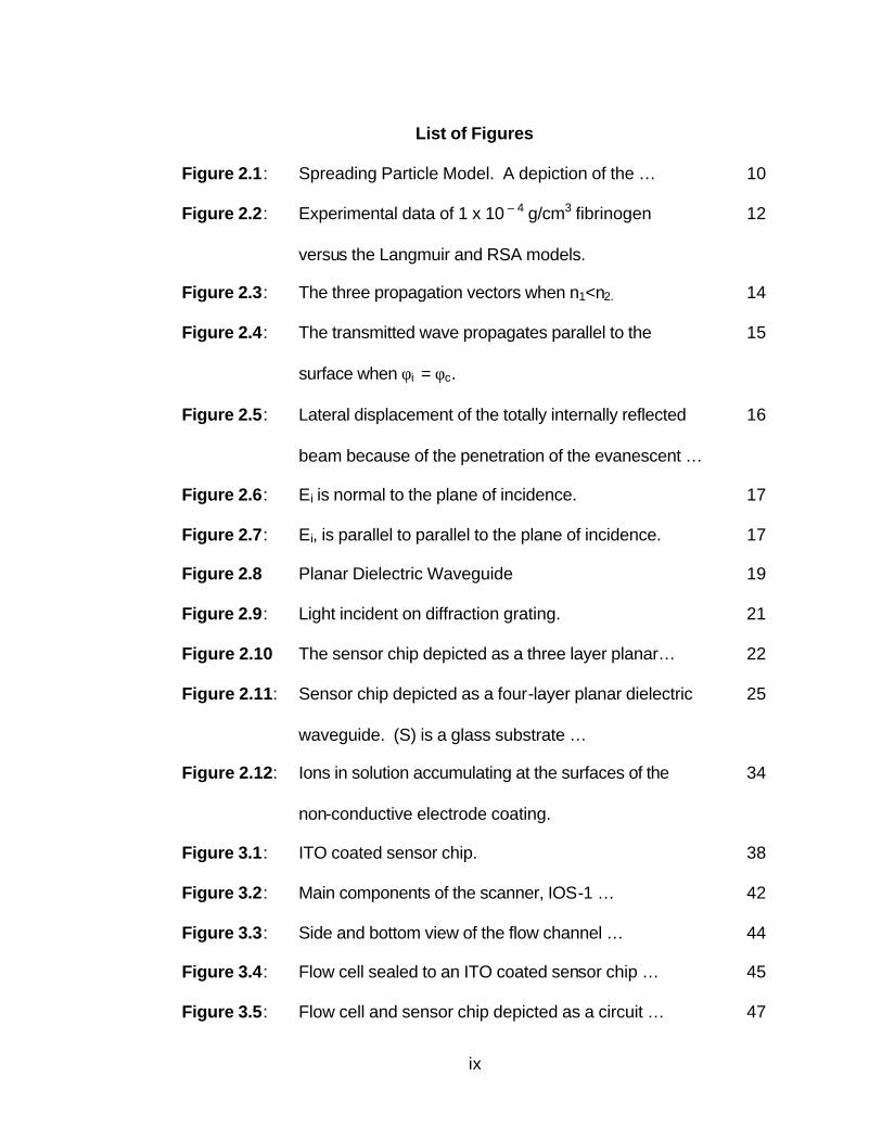
List of Figures

Figure 2.1: Spreading Particle Model. A depiction of the … 10

Figure 2.2: Experimental data of 1 x 10 – 4 g/cm3 fibrinogen 12

versus the Langmuir and RSA models.

Figure 2.3: The three propagation vectors when n1<n2. 14

Figure 2.4: The transmitted wave propagates parallel to the 15

surface when φi = φc.

Figure 2.5: Lateral displacement of the totally internally reflected 16

beam because of the penetration of the evanescent …

Figure 2.6: Ei is normal to the plane of incidence. 17

Figure 2.7: Ei, is parallel to parallel to the plane of incidence. 17

Figure 2.8 Planar Dielectric Waveguide 19

Figure 2.9: Light incident on diffraction grating. 21

Figure 2.10 The sensor chip depicted as a three layer planar… 22

Figure 2.11: Sensor chip depicted as a four-layer planar dielectric 25

waveguide. (S) is a glass substrate …

Figure 2.12: Ions in solution accumulating at the surfaces of the 34

non-conductive electrode coating.

Figure 3.1: ITO coated sensor chip. 38

Figure 3.2: Main components of the scanner, IOS-1 … 42

Figure 3.3: Side and bottom view of the flow channel … 44

Figure 3.4: Flow cell sealed to an ITO coated sensor chip … 45

Figure 3.5: Flow cell and sensor chip depicted as a circuit … 47

x

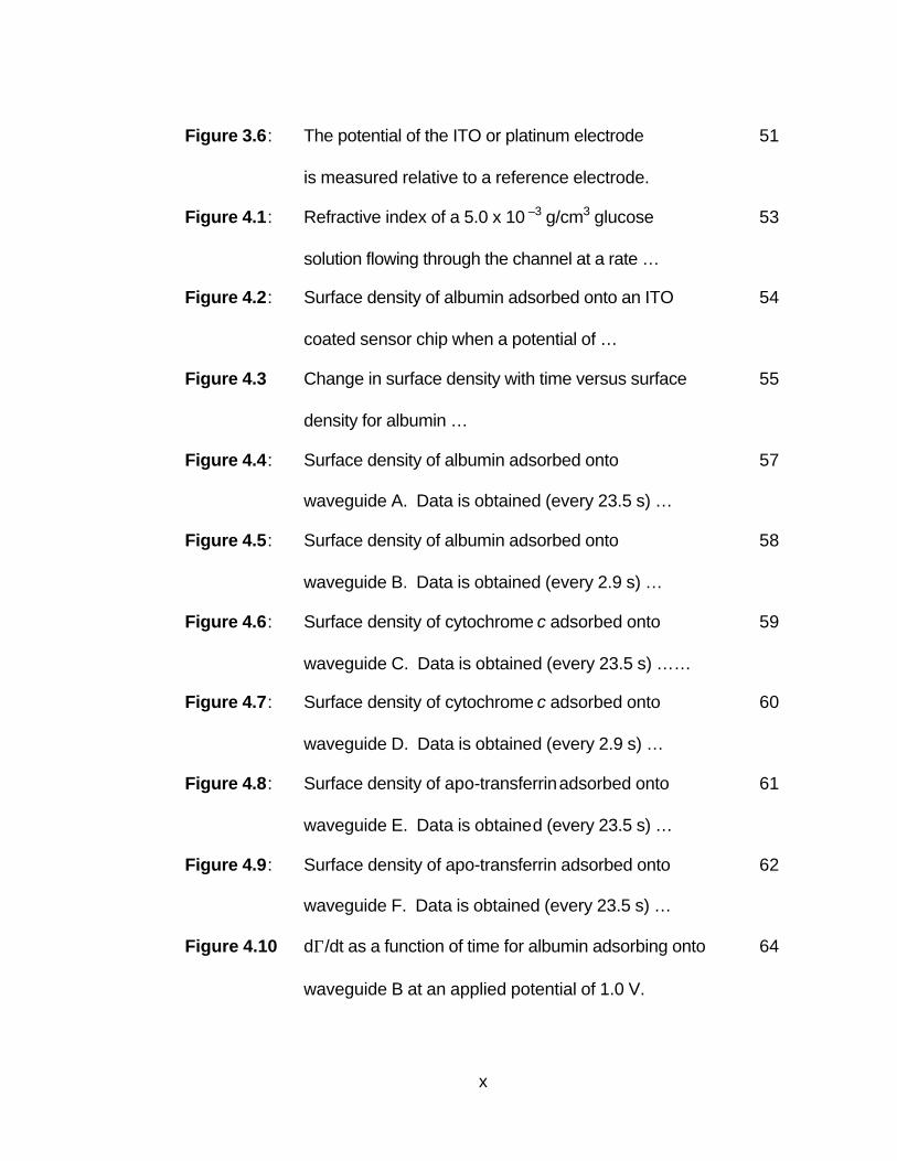
Figure 3.6: The potential of the ITO or platinum electrode 51

is measured relative to a reference electrode.

Figure 4.1: Refractive index of a 5.0 x 10 –3 g/cm3 glucose 53

solution flowing through the channel at a rate …

Figure 4.2: Surface density of albumin adsorbed onto an ITO 54

coated sensor chip when a potential of …

Figure 4.3 Change in surface density with time versus surface 55

density for albumin …

Figure 4.4: Surface density of albumin adsorbed onto 57

waveguide A. Data is obtained (every 23.5 s) …

Figure 4.5: Surface density of albumin adsorbed onto 58

waveguide B. Data is obtained (every 2.9 s) …

Figure 4.6: Surface density of cytochrome c adsorbed onto 59

waveguide C. Data is obtained (every 23.5 s) ……

Figure 4.7: Surface density of cytochrome c adsorbed onto 60

waveguide D. Data is obtained (every 2.9 s) …

Figure 4.8: Surface density of apo-transferrin adsorbed onto 61

waveguide E. Data is obtained (every 23.5 s) …

Figure 4.9: Surface density of apo-transferrin adsorbed onto 62

waveguide F. Data is obtained (every 23.5 s) …

Figure 4.10 dΓ/dt as a function of time for albumin adsorbing onto 64

waveguide B at an applied potential of 1.0 V.

xi

Figure 4.11 Adsorption rate dΓ/dt, as a function of time for 65

albumin…


cytochrome c….


apo-transferrin….

Figure 4.14: Change in surface density of adsorbed protein 68

with time verses density. Apparent initial …


with time verses density for albumin …


with time versus density for cytochrome c …


with time versus density for apo-transferrin …

Figure 4.18: The equilibrium constant, k, for albumin, 76

cytochrome c, and apo-transferrin ….

Figure 4.19: Surface density, as time goes to infinity, of albumin, 77

cytochrome c, and apo-transferrin ….

Figure 4.20: Density and current versus time for 1.0 x 10 – 4 g/cm3 78

albumin under a 2.0 V applied potential.

Figure 4.21: Current as a function of time during the adsorption 79

of albumin onto waveguides A and B.

xii


cytochrome c under a 2.0 V applied potential.


of cytochrome c onto waveguides C and D.


apo-transferrin under a 2.0 V applied potential


of apo-transferrin onto waveguides E and F.

Figure 4.26: Surface density of 1.0 x 10 – 4 g/cm3 albumin 86

adsorbed onto waveguide G …

Figure 4.27: Surface density of 1.0 x 10 – 4 g/cm3 cytochrome c 87

adsorbed onto waveguide H …

Figure B.1: Fibrinogen, 1.0 x 10 – 4 g/cm3, adsorbed onto a 103

Si0.25Ti0.75O2 film at a flow rate of …

Figure B.2: The effective refractive index, N(TE), measured 104

with time for deionized water flowing at a rate of …

Figure C.1: Experimental data of the refractive index of a 107

5.0 x 10 – 3 g/cm3 glucose solution flowing through

the channel at a rate of 1.33 x 10 – 3 cm3/s …

Figure C.2: Experimental data of the refractive index of a 108

5.0 x 10 –3 g/cm3 glucose solution flowing …

Figure D.1: Effective refractive indices of 1.0 x 10 – 4 g/cm3 109

human albumin adsorbing onto waveguide A…

xiii


human albumin adsorbing onto waveguide A.

At t = 300 s, 0.5 volts is applied to the …



At t = 360 s, 1.0 volts is applied to the…








human albumin adsorbing onto waveguide B

when no voltage is applied to the electrodes…

Figure D.7: Effective refractive index of 1.0 x 10 – 4 g/cm3 113

human albumin adsorbing onto waveguide B



human albumin adsorbing onto waveguide B.



human albumin adsorbing onto waveguide B…

xiv


human albumin adsorbing onto waveguide B.



cytochrome c adsorbing onto waveguide C

when no voltage is applied to the electrodes …


cytochrome c adsorbing onto waveguide C.



cytochrome c adsorbing onto waveguide C. At

t = 240 s, 1.0 volts is applied to the electrodes.

At t = 1740 s, the protein solution enters the …


cytochrome c adsorbing onto waveguide C. At




cytochrome c adsorbing onto waveguide C.



cytochrome c adsorbing onto waveguide D


xv


cytochrome c adsorbing onto waveguide D.









cytochrome c adsorbing onto waveguide D. At




apo-transferrin adsorbing onto waveguide E

when no voltage is applied to the electrodes.

At t= 600 s, the protein solution enters the …


apo-transferrin adsorbing onto waveguide E.





xvi





apo-transferrin adsorbing onto waveguide F



apo-transferrin adsorbing onto waveguide F.



apo-transferrin adsorbing onto waveguide F. At


At t = 1800s, the protein solution enters the …

Figure D.28: Current versus time during the adsorption of 126

human albumin onto waveguide A. At t = 300 s,

0.5 volts is applied to the electrodes. At t = 1800 s,

the protein solution enters the flow cell …



1.0 volts is applied to the electrodes …




xvii





human albumin onto waveguide B. At t = 300 s,














cytochrome c onto waveguide C. At t = 300 s,





xviii








cytochrome c onto waveguide D. At t = 300 s,














apo-transferrin onto waveguide E. At t = 300 s,


xix








apo-transferrin onto waveguide F. At t = 600 s,



apo-transferrin onto waveguide F. At t = 300 s,


Figure D.49: Effective refractive indices for 1.0 x 10 – 4 g/cm3 139

human albumin adsorbed onto waveguide G …

Figure D.50: Current as a function of time. At t = 300 s, 1.0 volts 140

is applied to the electrodes. At t= 2563 s, the …

Figure D.51: Potential of the ITO and platinum electrodes … 141

Figure D.52: Effective refractive indices for 1.0 x 10 – 4 g/cm3 142

cytochrome c adsorbing onto waveguide H…

Figure D.53: Current as a function of time. At t = 900 s, 1.0 volts 143

is applied to the electrodes. At t = 2845 s, the …

Figure D.54: Potential of the ITO and platinum electrodes 143

relative to a gold reference electrode. At …

1

1. Introduction

1.1 Problem Description

Proteins are biological macromolecules vital to cell structure and

function. The ability to incorporate proteins onto or within synthetic

materials offers the promise of new devices and processes of high potential

impact on the quality of human life. An important subclass of these

materials are those onto which a monolayer of protein molecules is

immobilized. Uses for such materials include supports for reusable

enzymes, thrombosis inhibiting biomaterials, bioelectric components, tissue

engineering substrates, and biosensing surfaces. The function of a surface-

immobilized protein monolayer depends critically on its structural properties;

these include lateral density, spatial homogeneity, relative molecular

orientation, and internal conformation. For example, surface-attached

enzymes (in catalysis) and matrix proteins (in cell attachment applications)

are oftentimes only effective if the proteins are oriented with their active sites

facing away from the surface and if the proteins retain (at least part of) their

native internal conformation. As a second example, layers of retinal

proteins, useful in photovoltaic devices, often function in a way that depends

critically on adsorbed layer uniformity.

Immobilizing protein monolayers with tailored structural properties

that could be independently optimized for a given application would be ideal.

In reality, we are far from this situation. Considering the diversity of systems

and applications, few established protein placement techniques exist.

2

A promising means for controlling the spatial homogeneity, mean

orientation, and growth rate of protein monolayers is through the application

of an external electric field. Due to a net charge and a permanent dipole,

most proteins align and migrate in an electric field.

Currently, little is known quantitatively of the effect of an electric field

on protein adsorption to a solid surface. One reason for this is the

experimental difficulty of simultaneously measuring adsorption and applying

the electric field. The purpose of this thesis is to develop a method for

following the time evolution of an adsorbed protein layer in the presence of

an electric field and to use this method to study the electric field dependence

of the adsorption kinetics of certain proteins.

1.2 Previous Work

Previous investigations of protein adsorption in the presence of an

external electric field have demonstrated an influence on adsorbed amounts,

orientation and antibody-antigen binding regulation by means of

electrochemical polarization [1, 2, 3, 4, 5].

Asanov, et al [1], studied the use of electrochemical polarization to

regulate antibody-antigen binding. Experiments were performed with biotin

covalently bound to an indium tin oxide electrode with strepavidin (or

polyclonal anti-biotin) subsequently adsorbed onto the biotinylated surface.

When no potential was applied to the ITO electrode (open circuit potential),

the irreversibly bound biotin-avidin (or antibody-antigen) complex

3

dissociated extremely slowly when rinsed with a pure buffer solution.

However, square wave polarization of the ITO electrode, -0.9 to +1.3 V for a

period of 5 s, during the rinse (time interval 2000-3000s) showed an

increase in the rate of dissociation and resulted in almost complete

regeneration of the biotinylated surface. Based on an earlier proposed

model, which assumed that with a variable double electric layer (DEL), a

protein molecule at the electrode surface would not have sufficient time to

adjust its structure and orientation to accommodate the new conditions and

thus rapidly desorb from the surface, it was concluded that a similar

mechanism could also describe the electrochemical stimulation of

dissociation of the biospecific complexes.

A study of the orientation of adsorbed cytochrome c as a function of

electrical potential of the adsorbing surface was presented by Fraaije, et al

[3]. Conclusions were that the adsorbed protein orientation on a tin oxide

electrode could only be affected when a potential was applied during the

adsorption process. No affect on orientation was observed when an

external potential was applied on previously adsorbed proteins.

Fievet, et al [4], studied the adsorption of a hydrophobic peptide onto

a carbon electrode. The adsorption was modeled by two consecutive

reactions occurring at the interface. The first reaction corresponded to the

irreversible adsorption of the peptide to the surface, and the second to a

change in conformation of the adsorbed molecules. Experimental conditions

were such that the peptide had an overall positive charge while the charge

4

of the surface was varied. It was determined that rate of adsorption and

coverage of molecules in an unaltered state (i.e. without a post-adsorption

change in conformation) and the coverage of molecules in an altered state

reached a maximum near the vicinity of a potential of zero charge, while the

rate of conformational change seemed to be independent of the charge of

the interface. It was suggested that because of the hydrophobic nature of

the peptide and carbon electrode (in addition to irreversible adsorption of the

peptide), the hydrophobic interactions were much stronger than the

coulombic interactions.

Bernabeu and Caprani [5] studied the adsorption of fibrinogen and

albumin onto the surface of a carbon electrode. Experimental conditions

were such that both proteins were negatively charged. It was found that the

density of protein adsorbed to the electrode increased with increasing

negative charge of the surface (i.e. the more negative the surface, the

greater the adsorption). To explain the favored adsorption of negative

proteins onto a negatively charged surface, it was proposed that cations

from the protein solvent adsorbed to the electrode surface creating a

positively charged layer with which the proteins could interact.

1.3 Approach

While previous research has established that an applied voltage can

have a significant impact on the adsorption process, it is difficult to draw

general conclusions from such studies. One reason for this is that the

5

kinetics of the adsorption process, from which much can be learned of the

underlying mechanisms, has not been systematically investigated. In this

work, it is proposed that a full kinetic analysis will allow one to determine the

affects of surface and protein charge and electrochemical properties of the

electrode surface on the adsorption process.

A method for measuring protein adsorption onto the surface of an

indium tin oxide (ITO) electrode based on Optical Waveguide Lightmode

Spectroscopy (OWLS) is developed. OWLS is a premier optical technique

that allows for the continuous measurement of adsorbed protein mass and

layer thickness, and shown by the results presented here, is capable of

yielding highly precise and accurate adsorption data over a range of applied

potentials. The proteins human albumin, cytochrome c, and apo-transferrin

are investigated in this work. These are chosen so that a range of size and

charge is considered.

6

2. Background

2.1 Basic Protein Chemistry

Proteins are biomolecules that are central to virtually every aspect of

cell structure and function [6]. Proteins can be thought of as medium

molecular weight flexible polymer chains. Chemically, proteins are linear

polymers of amino acids linked head to tail, from the carboxyl group to the

amino group, through covalent bonds.

Proteins can be assigned to one of three broad classes based on

their shape and solubility: fibrous, globular, and membrane. Fibrous

proteins are typically insoluble in water or dilute salt solutions, and tend to

have linear structures. Globular proteins, which are usually very soluble in

aqueous solutions, fold into compact units that are roughly spherical in

shape. Globular proteins tend to fold such that the hydrophobic amino acid

side chains are in the interior of the molecule while the hydrophilic side

chains are on the outside, exposed to the solvent. In contrast, membrane

proteins, which have their hydrophobic amino acid side chains oriented

outward, are characteristically insoluble in aqueous solutions.

The biological activity of proteins generally depends on their

conformation. The natural structure of proteins is dictated by (1) their amino

acid sequence, (2) their interaction with solvent molecules, and (3) the pH

and ionic composition of the solvent. Proteins tend to fold in such a way as

to form the most stable i.e. lowest free energy structure. Structural stability

primarily results from (1) the formation of large numbers of intramolecular

7

hydrogen bonds and (2) the reduction in surface area accessible to solvent

that occurs upon folding [6].

The ionic properties of proteins, determined primarily by their amino

acid side chains, are pH dependent. The pH value at which the sum of the

proteins positive and negative electrical charges is zero is the isoelectric

point, PI. At a pH value below the PI, the net charge of the protein is

positive. Charged residues are normally located on the surface of the

protein where they may interact with the solvent.

2.2 Protein Adsorption: Fundamental Principles

Most protein/surface combinations result in adsorption (i.e. sticking at

the interface). Physical adsorption at a liquid-solid interface is due to

favorable van der Waals, ionic and/or polar interactions. Most proteins

possess heterogeneous surfaces and may therefore exhibit more than one

mode of interaction with the adsorbing surface. The study of protein

adsorption onto solid surfaces is interesting theoretically and of practical

importance in areas such as (1) biocompatibility of materials, (2) separation

of biological solutions and (3) bioanalytical sensing.

2.3 Protein Adsorption: Theoretical Analysis

One would like to be able to predict the amount of protein adsorbed

to a surface as a function of time and certain protein and surface properties.

In flow experiments, protein molecules undergo convective diffusion toward

8

the surface. This is the rate limiting mechanism until a critical concentration

is established near the surface. However, in the absence of transport-

limitations, adsorption to the surface becomes the rate limiting process. In

this section, a few methods for predicting the adsorption rate under these

conditions are reviewed.

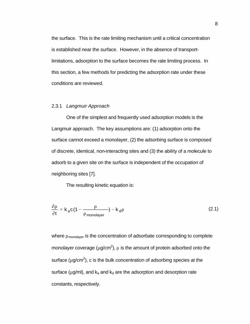
2.3.1 Langmuir Approach

One of the simplest and frequently used adsorption models is the

Langmuir approach. The key assumptions are: (1) adsorption onto the

surface cannot exceed a monolayer, (2) the adsorbing surface is composed

of discrete, identical, non-interacting sites and (3) the ability of a molecule to

adsorb to a given site on the surface is independent of the occupation of

neighboring sites [7].

The resulting kinetic equation is:

where ρmonolayer is the concentration of adsorbate corresponding to complete

monolayer coverage (µg/cm2), ρ is the amount of protein adsorbed onto the

surface (µg/cm2), c is the bulk concentration of adsorbing species at the

surface (µg/ml), and ka and kd are the adsorption and desorption rate

constants, respectively.

ρ−ρ

ρ−=∂ρ∂

dmonolayer

a k)1(ckt

(2.1)

9

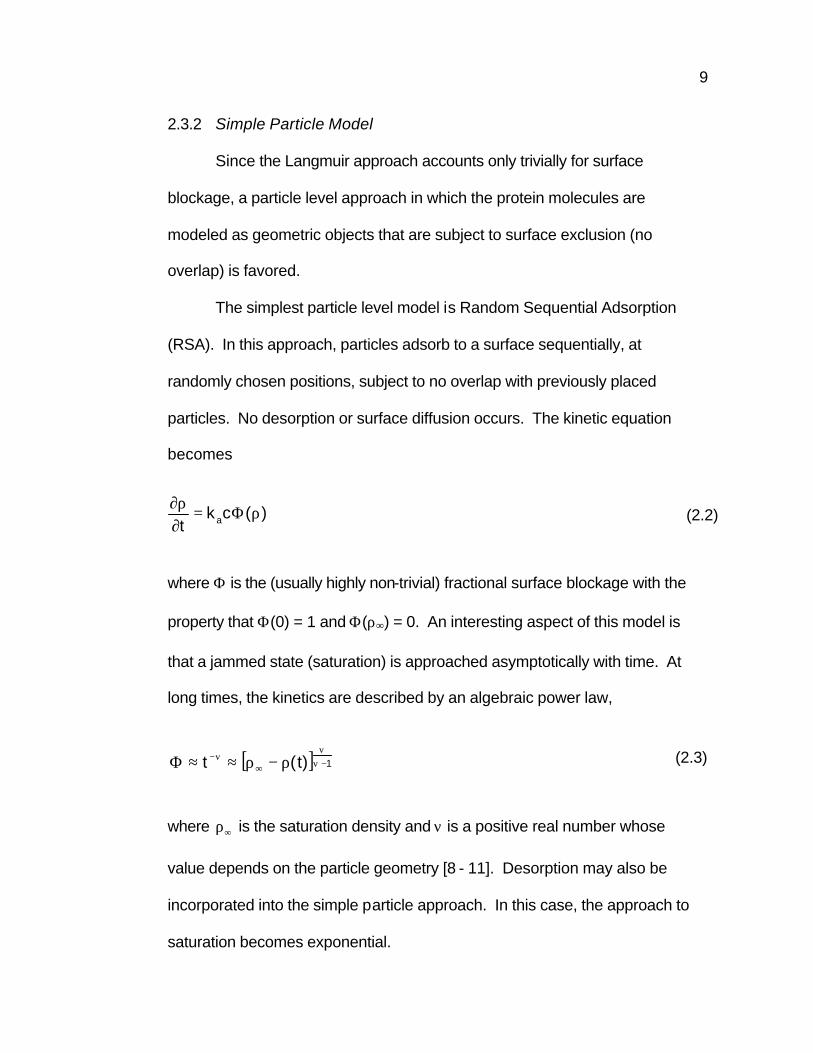
2.3.2 Simple Particle Model

Since the Langmuir approach accounts only trivially for surface

blockage, a particle level approach in which the protein molecules are

modeled as geometric objects that are subject to surface exclusion (no

overlap) is favored.

The simplest particle level model is Random Sequential Adsorption

(RSA). In this approach, particles adsorb to a surface sequentially, at

randomly chosen positions, subject to no overlap with previously placed

particles. No desorption or surface diffusion occurs. The kinetic equation

becomes

where Φ is the (usually highly non-trivial) fractional surface blockage with the

property that Φ(0) = 1 and Φ(ρ∞) = 0. An interesting aspect of this model is

that a jammed state (saturation) is approached asymptotically with time. At

long times, the kinetics are described by an algebraic power law,

where ∞ρ is the saturation density and ν is a positive real number whose

value depends on the particle geometry [8 - 11]. Desorption may also be

incorporated into the simple particle approach. In this case, the approach to

saturation becomes exponential.

(2.2) )(ckt a ρΦ=

∂ρ∂

[ ] 1)t(t −νν

∞ν− ρ−ρ≈≈Φ (2.3)

10

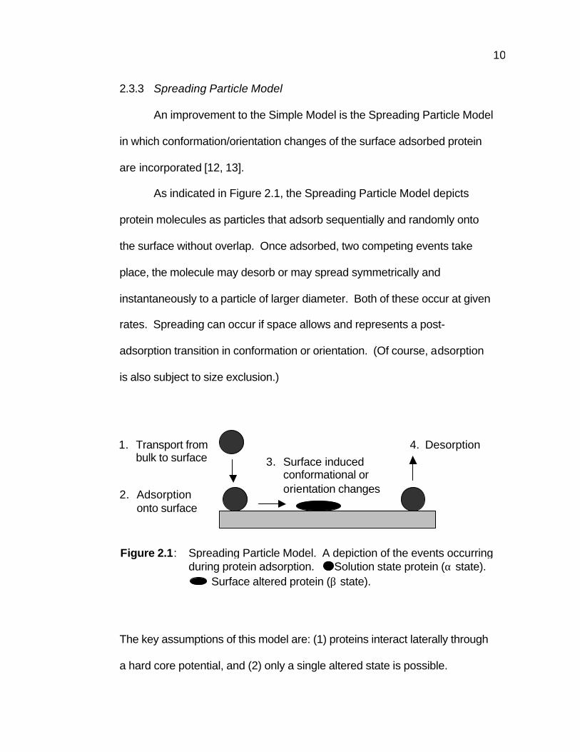
2.3.3 Spreading Particle Model

An improvement to the Simple Model is the Spreading Particle Model

in which conformation/orientation changes of the surface adsorbed protein

are incorporated [12, 13].

As indicated in Figure 2.1, the Spreading Particle Model depicts

protein molecules as particles that adsorb sequentially and randomly onto

the surface without overlap. Once adsorbed, two competing events take

place, the molecule may desorb or may spread symmetrically and

instantaneously to a particle of larger diameter. Both of these occur at given

rates. Spreading can occur if space allows and represents a post-

adsorption transition in conformation or orientation. (Of course, adsorption

is also subject to size exclusion.)

The key assumptions of this model are: (1) proteins interact laterally through

a hard core potential, and (2) only a single altered state is possible.

1. Transport from bulk to surface

2. Adsorption onto surface

3. Surface induced conformational or orientation changes

4. Desorption

Figure 2.1: Spreading Particle Model. A depiction of the events occurring during protein adsorption. Solution state protein (α state).

Surface altered protein (β state).

11

The kinetic equations for this process are

where ρα is the density of protein in the unspread state, ρβ is the density of

protein in the surface altered state, Φα is the adsorption probability

(fractional surface available for adsorption), Ψαβ is the spreading probability

(the probability that an already adsorbed molecule has sufficient space to

spread), ks is the spreading rate, ka and kd are the adsorption and desorption

rates, and c is the bulk concentration at the surface.

Assuming that the proteins (or more generally, “particles”) on the

surface are at all times in an equilibrium distribution, and that their surface

projections are disk shaped, analytical expressions for the adsorption and

spreading probabilities may be derived via the Scaled Particle Theory [14,

15]. (See Appendix A for details.)

2.3.4 Adsorption Model Curves

Both Langmuir and Particle Models predict an initial linear increase in

adsorbed amounts with a slope proportional to the surface concentration.

The approach to saturation of the Langmuir Model is strictly exponential,

αβα Ψρ−ρ−Φ=∂ρ∂

ααα

sd kkckt a

(2.4)

αβαβ Ψρ=

∂ρ∂

skt

(2.5)

12

and thus very fast. In the Particle Model, this approach is much slower due

to the more realistic manner in which the surface is blockage is treated. (In

the case of purely irreversible adsorption, the approach is algebraic, i.e.

ν−∞ ≈ρ−ρ t)t()( .) These models may be coupled to transport models that

predict the bulk concentration near the surface as a function of time and flow

conditions [16].

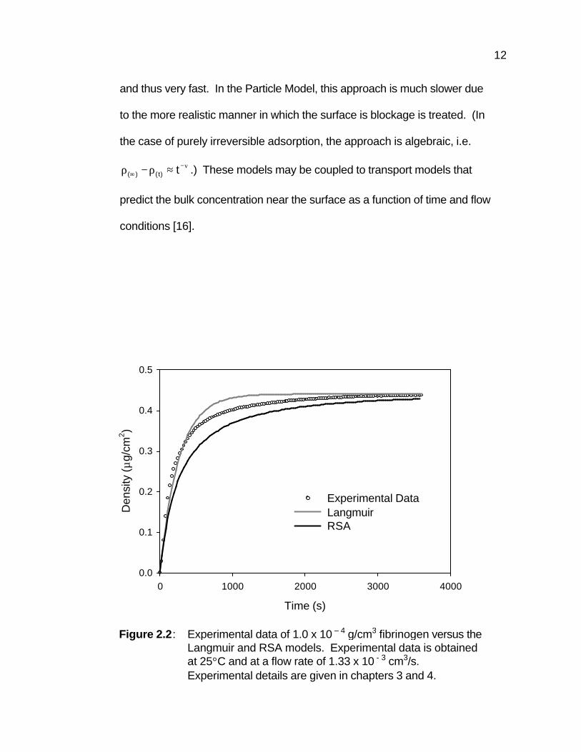
Figure 2.2: Experimental data of 1.0 x 10 – 4 g/cm3 fibrinogen versus the

Langmuir and RSA models. Experimental data is obtained at 25°C and at a flow rate of 1.33 x 10 - 3 cm3/s. Experimental details are given in chapters 3 and 4.

Time (s)

0 1000 2000 3000 4000

Den

sity

(µg/

cm2 )

0.0

0.1

0.2

0.3

0.4

0.5

Experimental DataLangmuirRSA

13

2.4 Adsorption Measurement Technique

There are a number of techniques used to measure the amount of

protein adsorbed onto a surface. Some of these are based on optical

principals, for example, Optical Waveguide Lightmode Spectroscopy, Total

Internal Reflection Fluorescence, Scanning Angle Reflectometry, and

Ellipsometry. Non-optical methods also exist, such as Quartz Crystal

Microbalance, which is based on a weight measurement. Each of these

methods or techniques offers various advantages (and, of course,

disadvantages). Total Internal Reflection Fluorescence requires proteins

with either a natural or attached fluorescent label. Quartz Crystal

Microbalance requires careful accounting of viscous drag of the contacting

liquid. In contrast, Optical Waveguide Lightmode Spectroscopy suffers from

neither of the problems and has been shown to provide accurate and

precise kinetic adsorption data for several protein/surface systems [17 - 20].

In this work, Optical Waveguide Lightmode Spectroscopy is used to obtain

continuous measurements of surface adsorbed protein.

2.4.1 Propagation of Light

Light propagates through space in a wave-like nature and yet, during

the processes of absorption and emission, behaves in a particle-like fashion.

The wave nature of light can be represented by the classical

electromagnetic field equations of Maxwell. Consider light (in the form of a

plane wave) impinging on an optical material. The boundary conditions of

14

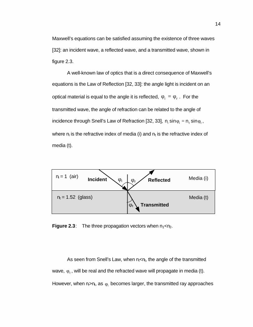
Maxwell’s equations can be satisfied assuming the existence of three waves

[32]: an incident wave, a reflected wave, and a transmitted wave, shown in

figure 2.3.

A well-known law of optics that is a direct consequence of Maxwell’s

equations is the Law of Reflection [32, 33]: the angle light is incident on an

optical material is equal to the angle it is reflected, ri φ=φ . For the

transmitted wave, the angle of refraction can be related to the angle of

incidence through Snell’s Law of Refraction [32, 33], ttii sinnsinn φ=φ ,

where ni is the refractive index of media (i) and nt is the refractive index of

media (t).

As seen from Snell’s Law, when ni<nt, the angle of the transmitted

wave, tφ , will be real and the refracted wave will propagate in media (t).

However, when ni>nt, as iφ becomes larger, the transmitted ray approaches

Figure 2.3: The three propagation vectors when n1<n2.

φr Reflected

φ t Transmitted

Incident φ i

nt = 1.52 (glass)

ni = 1 (air) Media (i)

Media (t)

15

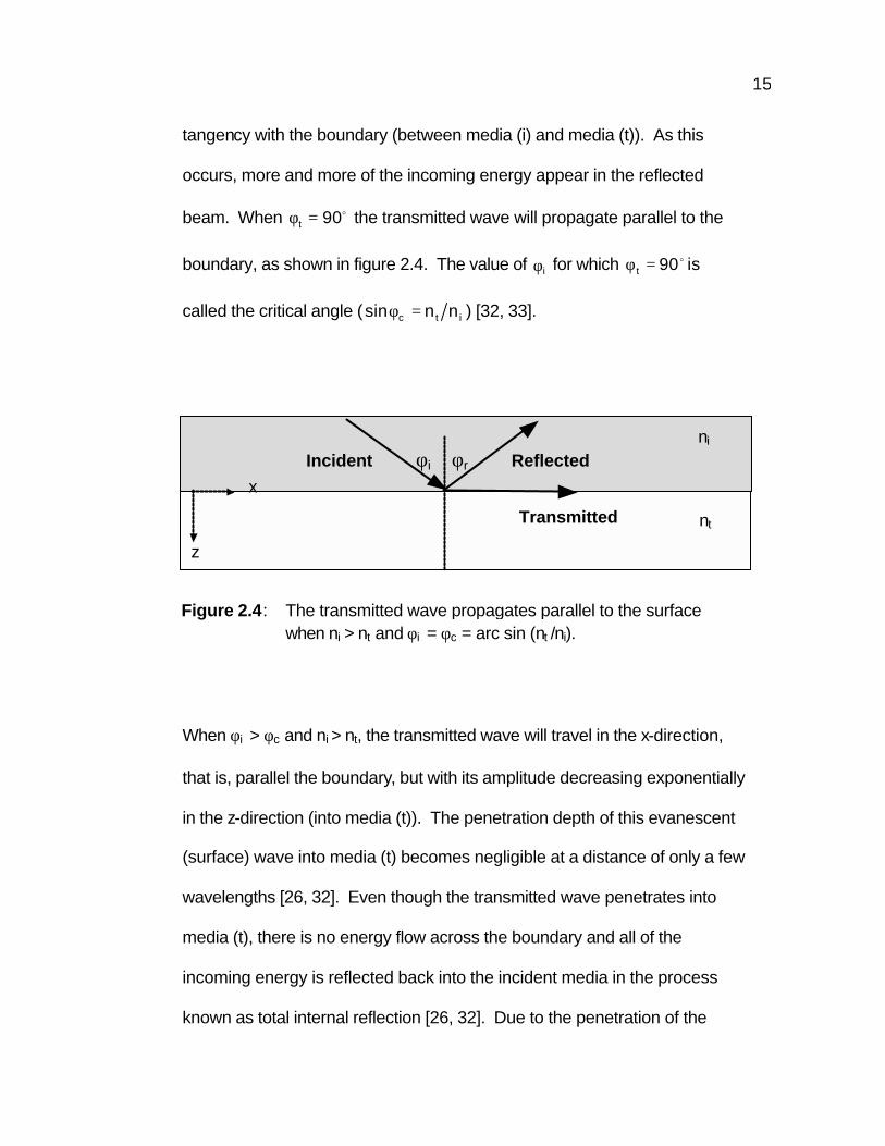
tangency with the boundary (between media (i) and media (t)). As this

occurs, more and more of the incoming energy appear in the reflected

beam. When o90t =φ the transmitted wave will propagate parallel to the

boundary, as shown in figure 2.4. The value of iφ for which o90t =φ is

called the critical angle ( itc nnsin =φ ) [32, 33].

When φi > φc and ni > nt, the transmitted wave will travel in the x-direction,

that is, parallel the boundary, but with its amplitude decreasing exponentially

in the z-direction (into media (t)). The penetration depth of this evanescent

(surface) wave into media (t) becomes negligible at a distance of only a few

wavelengths [26, 32]. Even though the transmitted wave penetrates into

media (t), there is no energy flow across the boundary and all of the

incoming energy is reflected back into the incident media in the process

known as total internal reflection [26, 32]. Due to the penetration of the

Figure 2.4: The transmitted wave propagates parallel to the surface when ni > nt and φi = φc = arc sin (nt /ni).

φr Reflected

Transmitted

Incident φ i ni

nt

z

x

16

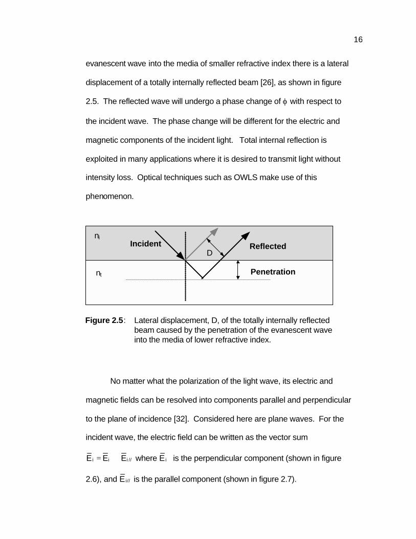
evanescent wave into the media of smaller refractive index there is a lateral

displacement of a totally internally reflected beam [26], as shown in figure

2.5. The reflected wave will undergo a phase change of ϕ with respect to

the incident wave. The phase change will be different for the electric and

magnetic components of the incident light. Total internal reflection is

exploited in many applications where it is desired to transmit light without

intensity loss. Optical techniques such as OWLS make use of this

phenomenon.

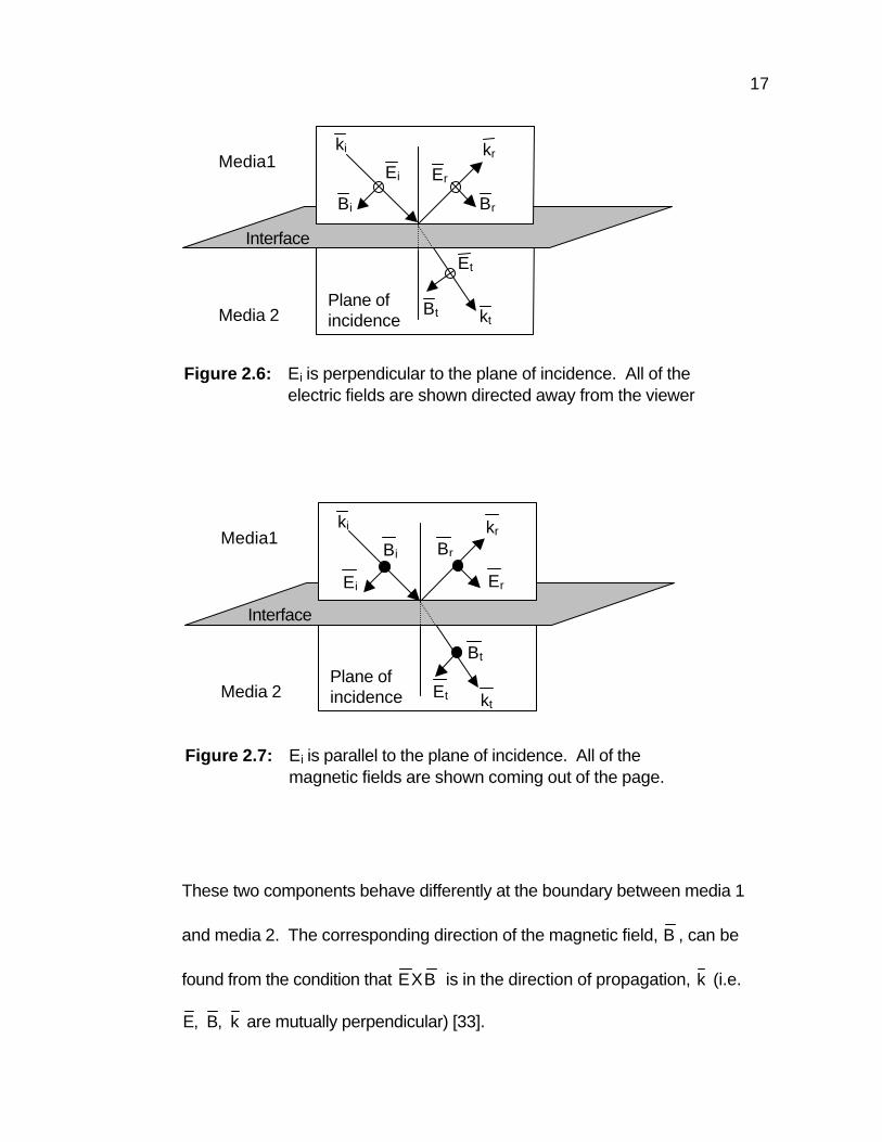
No matter what the polarization of the light wave, its electric and

magnetic fields can be resolved into components parallel and perpendicular

to the plane of incidence [32]. Considered here are plane waves. For the

incident wave, the electric field can be written as the vector sum

//iii EEE += ⊥ where ⊥iE is the perpendicular component (shown in figure

2.6), and //iE is the parallel component (shown in figure 2.7).

Figure 2.5: Lateral displacement, D, of the totally internally reflected beam caused by the penetration of the evanescent wave into the media of lower refractive index.

Incident ni

nt

Reflected

Penetration

D

17

These two components behave differently at the boundary between media 1

and media 2. The corresponding direction of the magnetic field, B , can be

found from the condition that BXE is in the direction of propagation, k (i.e.

k,B,E are mutually perpendicular) [33].

Figure 2.6: Ei is perpendicular to the plane of incidence. All of the electric fields are shown directed away from the viewer

Interface

Plane of incidence

Media1

Media 2

ki

Er

Ei

Et

Bi Br

Bt

kr

kt

Interface

Plane of incidence

Media1

Media 2

ki

Br

Bt

Bi

Ei Er

Et kt

kr

Figure 2.7: Ei is parallel to the plane of incidence. All of the magnetic fields are shown coming out of the page.

18

The interdependence of the amplitudes of the incident, reflected, and

transmitted waves is shown by Fresnel’s equations that evaluate the

amplitude reflection coefficient, ioro EE , and the amplitude transmission

coefficient, ioto EE [26, 32, 33]. The Fresnel equations obtained for the

electric field being perpendicular to the plane of incidence and that in which

it is parallel provides a means to determine the phase shift, TETM and ϕϕ ,

associated with total internal reflection.

2.4.2 Optical Waveguides

Of practical importance is the confinement and propagation of light

through optical waveguides. The key to high-speed telecommunications is

the transmission of visible or infrared light that has been modulated with a

signal, through small optical fibers. Optical Waveguide Lightmode

Spectroscopy, the technique used in this work to study protein adsorption,

utilizes a sensor chip that is also a dielectric waveguide. An import aspect

of such waveguides is that light can be transmitted over a long distance with

little loss of intensity.

Consider a simple planar waveguide consisting of a dielectric film of

thickness df in the z-direction and infinite in the other two directions. A

dielectric media, M, of refractive index nm surrounds the film, F, which has a

refractive index value of nf, where nf > nm. Figure 2.8 shows light confined

inside of the film as it propagates in the x-direction. Geometrically, any ray

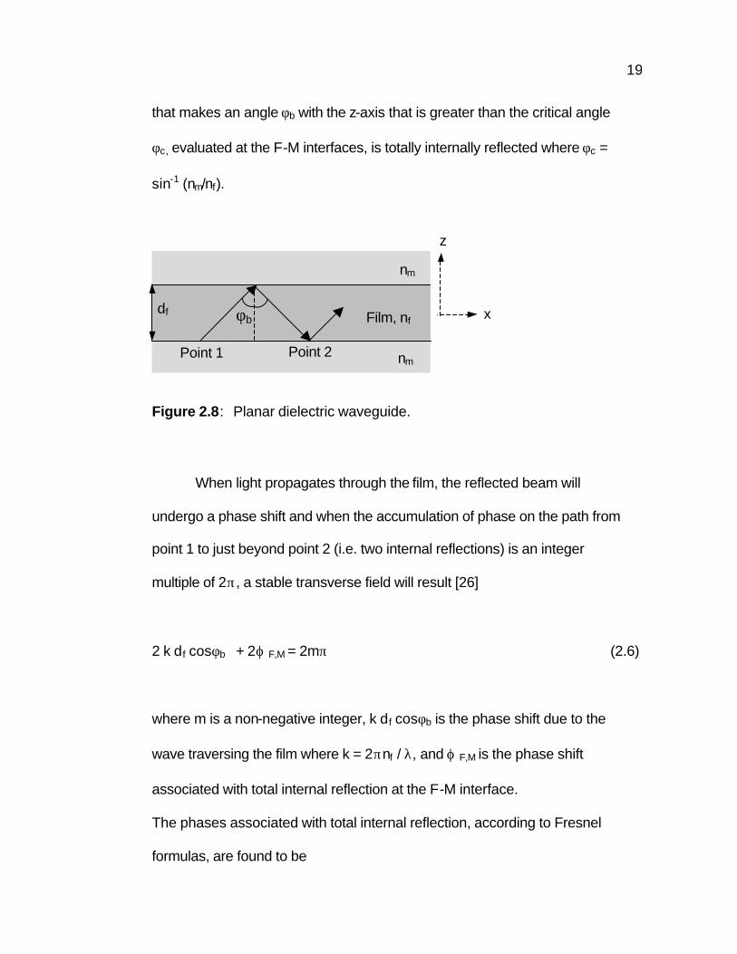
19

that makes an angle φb with the z-axis that is greater than the critical angle

φc, evaluated at the F-M interfaces, is totally internally reflected where φc =

sin-1 (nm/nf).

When light propagates through the film, the reflected beam will

undergo a phase shift and when the accumulation of phase on the path from

point 1 to just beyond point 2 (i.e. two internal reflections) is an integer

multiple of 2π, a stable transverse field will result [26]

2 k df cosφb + 2ϕ F,M = 2mπ

where m is a non-negative integer, k df cosφb is the phase shift due to the

wave traversing the film where k = 2πnf / λ, and ϕ F,M is the phase shift

associated with total internal reflection at the F-M interface.

The phases associated with total internal reflection, according to Fresnel

formulas, are found to be

Film, nf

nm

nm

φb df

Point 1 Point 2

x

z

Figure 2.8: Planar dielectric waveguide.

(2.6)

20

where the subscripts TE and TM correspond to the electric field component

of the light being perpendicular and parallel to the plane of incidence,

respectively. For a given value of the propagation angle, φb, the phases for

the TM mode will differ from that of TE. Therefore, equation 2.6 will equal

2mπ at a different propagation angles for the TE mode than the TM mode.

2.4.3 Optical Waveguide Lightmode Spectroscopy

Optical Waveguide Lightmode Spectroscopy (OWLS) [21 - 25] is a

technique, based on multiple total internal reflections, that is used to study

the adsorption of protein or other macromolecules onto the surface of a

sensor chip. The sensor chip is comprised of a glass substrate coated with

a thin, optically transparent, metal oxide film and a relief grating embossed

into the film’s surface. Polarized light from a He-Ne laser is directed onto

the sensor chip at the grating region. The sensor chip is rotated between ±

12.6° relative to the fixed laser beam. At a well-defined angle, α, light from

the laser is coupled into the film of the sensor chip by means of the grating.

(2.7)

φ−

−φ

−=ϕ

5.0

b22

f2f

2mb

22f

2

m

f)TM(M,F

sinnn

nsinnnn

arctan2

(2.8)

φ−

−φ−=ϕ

5.0

b22

f2f

2mb

22f

)TE(M,Fsinnn

nsinnarctan2

21

The incoupled light propagates through the film via multiple total internal

reflections. The intensity of light coupled out of the film is detected by

photodectors (one located at each end of the chip) and is recorded as a

function of the incident angle of the laser beam. The incident angles at

which light is maximally coupled into the film of the sensor chip are the basic

physical values determined by the biosensing system.

When light impinges on a diffraction grating (figure 2.9) it is scattered

and multiple diffracted beams b = 0, b = 1± … will arisen according to [33]

Λλ

=φ−φb

sinnsinn ifbf

where b is the order of the diffraction grating, λ is the wavelength of the

incident laser, and 1/Λ is the grating period.

For a diffracted beam to be coupled inside of the film of the sensor chip

(which is depicted in figure 2.10 as a three layer waveguide) and propagate,

the angle at which the light is diffracted must be greater than the critical

angles (evaluated at each interface), that is φb > φc (F,S) and φb > φc (F,C). If

(2.9)

φb φi 1st order (b = -1)

0 th order (b = 0)

1st order (b = +1)

Media of refractive index nf

Diffraction Grating

Figure 2.9: Light incident on a diffraction grating

22

cb φ<φ , total internal reflection will not occur. The sensor chips used in

OWLS are designed so that only one diffracted beam is coupled into the

waveguiding film. This is due to the grating period of the diffraction grating

and the refractive index of the waveguiding film.

From the diffraction equation (2.9), an effective refractive index, N, for

either the TE or TM mode of polarization is defined as [21, 22]

Λλ

±α=φ=±b

sinnsinnN airbf (2.10)

-x

Figure 2.10: The sensor chip is depicted as a three layer planar dielectric waveguide: (S) is a glass substrate, (F) is a thin film onto which a diffraction grating is embossed, and (C) is a media that is in contact with the film at the grating region.

+x

Laser

φ i

Grating

φb

nc C

nf

γs

α nair

S ns

F

23

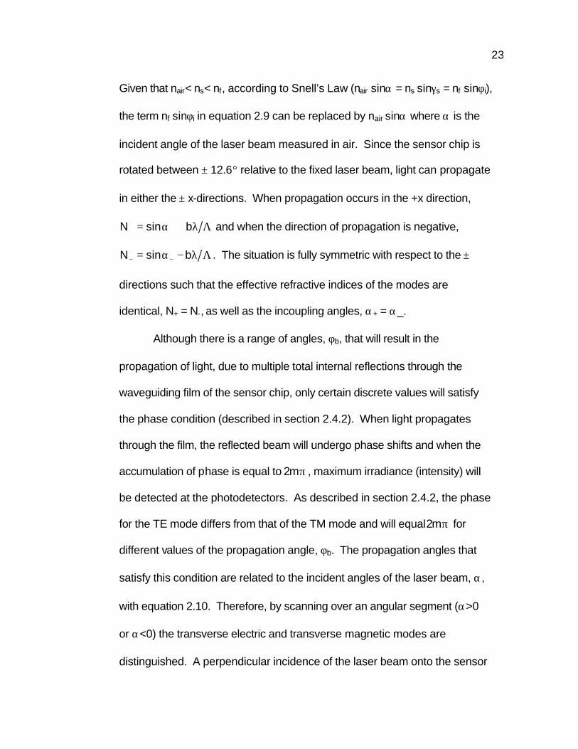
Given that nair< ns< nf, according to Snell’s Law (nair sinα = ns sinγs = nf sinφi),

the term nf sinφi in equation 2.9 can be replaced by nair sinα where α is the

incident angle of the laser beam measured in air. Since the sensor chip is

rotated between ± 12.6° relative to the fixed laser beam, light can propagate

in either the ± x-directions. When propagation occurs in the +x direction,

Λλ+α= ++ bsinN and when the direction of propagation is negative,

Λλ−α= −− bsinN . The situation is fully symmetric with respect to the ±

directions such that the effective refractive indices of the modes are

identical, N+ = N-, as well as the incoupling angles, α+ = α_.

Although there is a range of angles, φb, that will result in the

propagation of light, due to multiple total internal reflections through the

waveguiding film of the sensor chip, only certain discrete values will satisfy

the phase condition (described in section 2.4.2). When light propagates

through the film, the reflected beam will undergo phase shifts and when the

accumulation of phase is equal to πm2 , maximum irradiance (intensity) will

be detected at the photodetectors. As described in section 2.4.2, the phase

for the TE mode differs from that of the TM mode and will equal πm2 for

different values of the propagation angle, φb. The propagation angles that

satisfy this condition are related to the incident angles of the laser beam, α,

with equation 2.10. Therefore, by scanning over an angular segment (α>0

or α<0) the transverse electric and transverse magnetic modes are

distinguished. A perpendicular incidence of the laser beam onto the sensor

24

chip results in a standing wave of light such that propagation through the

film occurs both in the +x and –x directions. The angular position halfway

between two peaks of light intensity (one peak resulting from light

propagating in the +x direction and the other in the –x direction) of the same

polarization is the angle of autocollimation. When light is coupled into the

waveguiding film, the angular position of the resonance peaks of light

intensity corresponding to the (TE ± ) and (TM ± ) modes along with the

angle of autocollimation is used to determine the incoupling angles for the

different modes. For reasons of symmetry α(TE+)=α(TE-) and

α(TM+)=α(TM-). [25]

When a protein solution is brought in contact with the film of the

sensor chip, as illustrated in Figure 2.11, the propagation angle changes

due to result the adsorption of molecules onto the film surface. The

propagation angle, φb, which is dependent on the optical properties of the

sensor chip (film and substrate) as well as on the surrounding media, is

related to the incoupling angle, α, by equation 2.10. Therefore, by

monitoring the incoupling angles, the amount of surface adsorbed protein

can be determined.

2.4.4 Sensor Chips

The theory of integrated optics for planar dielectric waveguides is

used to compute the refractive index and thickness, as a function of time, of

a protein layer deposited onto the film surface of the sensor chip. The

25

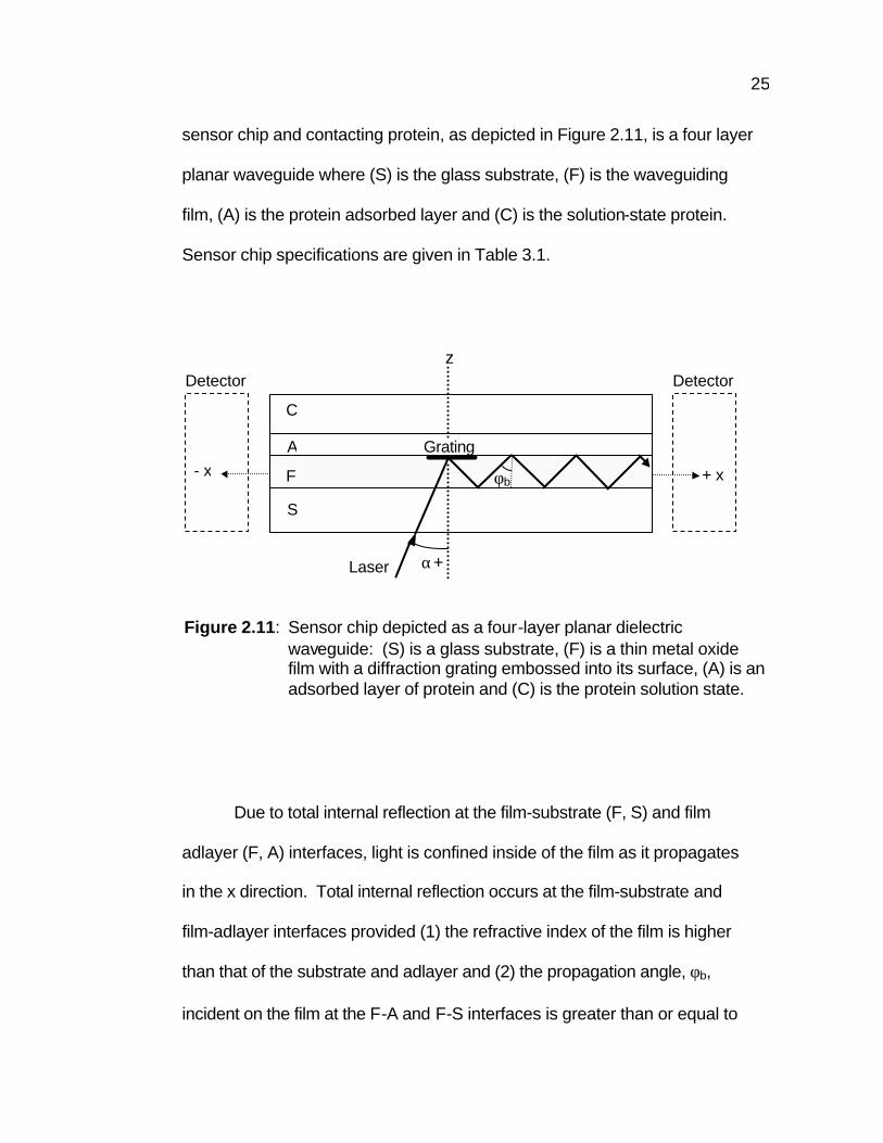
sensor chip and contacting protein, as depicted in Figure 2.11, is a four layer

planar waveguide where (S) is the glass substrate, (F) is the waveguiding

film, (A) is the protein adsorbed layer and (C) is the solution-state protein.

Sensor chip specifications are given in Table 3.1.

Due to total internal reflection at the film-substrate (F, S) and film

adlayer (F, A) interfaces, light is confined inside of the film as it propagates

in the x direction. Total internal reflection occurs at the film-substrate and

film-adlayer interfaces provided (1) the refractive index of the film is higher

than that of the substrate and adlayer and (2) the propagation angle, φb,

incident on the film at the F-A and F-S interfaces is greater than or equal to

Figure 2.11: Sensor chip depicted as a four-layer planar dielectric waveguide: (S) is a glass substrate, (F) is a thin metal oxide film with a diffraction grating embossed into its surface, (A) is an adsorbed layer of protein and (C) is the protein solution state.

C

F

A

S

z

- x + x

Grating

α+

φb

Laser

Detector Detector

26

the critical angles, φc, at each of the two interfaces [φb ≥ φc (F,A) and φb ≥ φc

(F,S)]. Since the penetration depth of the evanescent (surface) wave into the

less dense media (S and A) is of a few wavelengths, the cover media needs

to be considered when the adlayer thickness is less than (or of the same

order of magnitude as) the wavelength of light. In the following discussion it

is given that φb >sin-1 (nC/nF) and φb >sin-1 (nS/nF) = φc (F,S).

A stable traverse field and coherent propagation in the x-direction will

result (i.e. maximum intensity will be detected) when the propagation

condition is satisfied

where k z,F d F is the phase shift due to the wave traversing the film, ϕ F,S and

ϕ F,A,C are the phases associated with total internal reflection at the film-

substrate and film-adlayer interfaces, respectively.

When N < nF and N > nA (i.e. φf >sin -1(nA/nF) = φc (F, A)), the

mathematical expressions for these phases are:

m2dk2 C,A,FS,FFF,z π=ϕ+ϕ+ (2.11)

−−

−=ϕ

2/1

22F

2S

2p2

S

FS,F Nn

nNnn

arctan2(2.11 a)

−+

−−

−=ϕ

)dk2exp(ba

)dk2exp(ba

k

k

nn

arctan2AA,z

AA,z

F,z

A,zp2

A

FC,A,F

(2.11 b)

27

where

N is the effective refractive index of a guided mode of polarization (TE or

TM), nf and df are the refractive index and thickness of the film, nA and dA

are the refractive index and thickness of the protein adsorbed layer, ns is the

refractive index of the substrate, nc is the refractive index of the cover

media, and p is a number equal to zero or one. To obtain the expressions

for the transverse electric mode of polarization one sets p = 0. The

expressions for the transverse magnetic mode are obtained by setting p = 1.

In the above expression of ϕ F,A,C, it is assumed that the adlayer (protein

adsorbed layer) is a homogeneous monolayer. This assumption is

reasonable if the surface heterogeneity is on a length scale smaller than the

light.

When N < nF and N < nA the mathematical expressions for the

phases are:

2/122FF,z )Nn(

2k −

λπ

= p2C

C,zp2

A

A,z

n

k

n

ka +=

2/12A

2A,z )nN(

2k −

λπ

= p2C

C,z

p2A

A,z

n

k

n

kb −=

−−

−=ϕ

2/1

22F

2S

2p2

S

FS,F Nn

nNnn

arctan2 (2.11 c)

28

where

The sensor chips used with the biosensor support only the zeroth

modes of polarization, therefore m=0 in equation (2.11). The number of

modes supported by the waveguide can be approximated from the one-

dimensional phase-space estimate [26].

NOTE and NOTM are the number of transverse electric and transverse

magnetic modes supported by the waveguide, φb is the propagation angle,

φc is the critical angle at the film interface, fd is the film thickness, and k is

the propagation number. For example, if 3NN OTMOTE =≈ , the waveguide

( )oo 90

2f90

ff

k

k

zfOTMOTE

cc

max

min

sin1kd

coskd

2k

dNNθφ

φ−π

−=θ∂

π−

=π

∂≈≈ ∫∫ (2.12)

2/122FF,z )Nn(

2k −

λπ

=2/122

AA,z )Nn(2

k −λπ

=

−−

−=ϕ

2/1

22A

2C

2p2

c

AC,A Nn

nNnn

arctan2

ϕ+

=ϕ

2dktan

kk

nn

arctan2 C,AAA,z

F,z

A,zp2

A

FC,A,F

(2.11 d)

29

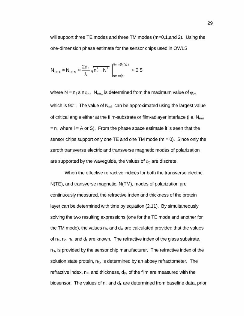
will support three TE modes and three TM modes (m=0,1,and 2). Using the

one-dimension phase estimate for the sensor chips used in OWLS

where bf sinnN φ= . Nmax is determined from the maximum value of φb,

which is 90°. The value of Nmin can be approximated using the largest value

of critical angle either at the film-substrate or film-adlayer interface (i.e. Nmin

= ni, where i = A or S). From the phase space estimate it is seen that the

sensor chips support only one TE and one TM mode (m = 0). Since only the

zeroth transverse electric and transverse magnetic modes of polarization

are supported by the waveguide, the values of φb are discrete.

When the effective refractive indices for both the transverse electric,

N(TE), and transverse magnetic, N(TM), modes of polarization are

continuously measured, the refractive index and thickness of the protein

layer can be determined with time by equation (2.11). By simultaneously

solving the two resulting expressions (one for the TE mode and another for

the TM mode), the values nA and dA are calculated provided that the values

of ns, nc, nf, and df are known. The refractive index of the glass substrate,

nS, is provided by the sensor chip manufacturer. The refractive index of the

solution state protein, nC, is determined by an abbey refractometer. The

refractive index, nF, and thickness, dF, of the film are measured with the

biosensor. The values of nF and dF are determined from baseline data, prior

( )

( )

5.0Nnd2

NN)(fnminN

nmaxN

22f

fOTMOTE

c

f

≈−λ

≈≈φ

30

to the onset of protein adsorption using the two expressions obtained by

equation (2.11), where nA is set equal to nC and dA is set equal to zero.

For given values of nA, and dA, the density of protein adsorbed onto

the surface of the film can be calculated by assuming a uniform layer of

constant density, of thickness dA, and of refractive index nA [21]:

where ρ is the surface density of protein adsorbed onto the film, and dn/dc,

which can be determined experimentally with a refractometer, is the change

in refractive index of a bulk solution with a change in concentration. For

many proteins, a linear dependence is observed with dn/dc=1.88 x 10 – 1

cm3/g over a large concentration range.

When the effective refractive index for only one of the two modes of

polarization is continuously measured, the density of adsorbed protein can

be determined with time. Assuming the values of nA and nC are constant

[21]

where ∆N is the change in the effective refractive indices resulting from

protein adsorption and

(2.14)

cn

NNd

)nn( ACA

∂∂

∆∂∂

−=ρ

( )

cn

dnn ACA

∂∂

−=ρ (2.13)

31

p

1)nN()nN(1)nN()nN(

)nn()nn(

dN

dN

2F

2C

2A

2C

2C

2F

2C

2A

FA

−+−+

−−

∂∂=

∂∂

( )

−

+

−

πλ+

−=

∂∂

∑=

−

−

C,SJ

2

J

2

F

2/12J

2F

22F

Fp

1nN

nN

nN2

dN

)Nn(dN

In equation 2.14 b, J = S or C corresponding the cover media and

substrate. To obtain the expressions for the transverse magnetic mode of

polarization one sets p equal to 1. Similarly, p is set equal to zero for the

transverse electric mode

Optical Waveguide Lightmode Spectroscopy provides a means to

measure the rate and amount of surface adsorbed protein. The rate at

which protein adsorbs to a surface is governed by diffusion and protein

surface interactions. In this work, the adsorption kinetics of protein in an

external electric field is studied to determine if the rate, saturation density

and adsorbed state can be influenced.

2.5 Electric Field Systems

A promising means for controlling the mean orientation and growth

rate of protein monolayers is through the application of an electric field. Due

(2.14 a)

(2.14 b)

32

to a net charge and a permanent dipole, most proteins align and migrate in

an electric field. An electric field will exert a force on any charge that is

present in the field. Positive charges will experience a force in the direction

of the field and negative charges in the opposite direction, where the force

on a unit of charge, q, is

Polar molecules will align or orient themselves in an electric field due to

torque resulting from forces acting on charges throughout the molecule.

Currently, little is known quantitatively of the effect of an electric field

on protein adsorption to a solid surface. One reason is the experimental

difficulty of simultaneously measuring adsorption and applying the electric

field. To investigate the influence of an electric field on protein adsorption

using OWLS, the limitations posed by the measurement technique must be

understood.

The sensor chips used in the biosensor provide a surface onto which

protein adsorbs. To examine the effect of an electric field on adsorption, it is

desired that the direction of the field be perpendicular to the adsorbing

surface. With this configuration, the electric field forces acting on the

molecule should oppose or act in the direction of diffusion (toward the

surface). An electric field between two oppositely charged parallel plates is

constant in magnitude and directed normal to the plates. The electric field

strength is then

EqFrr

= (2.15)

33

zd

VE plates∆

=

where ∆Vplates is the voltage difference between the plates and d is their

separation.

To create a perpendicular electric field, a thin conducting layer must

be placed on the waveguide. This allows the sensor chip to act as one of

the conducting plates in a parallel plate setup. So long as the conducting

layer is extremely thin and its conductivity relatively low the theory of

integrated optics for planar dielectric waveguides can be applied, as

demonstrated in Section 3.3.2 of this work, to calculate the amount of

surface adsorbed protein.

Proteins are usually dissolved in a buffer solution of relatively high

ionic strength. When an electrolytic solution is placed between the plates,

ions will in solution will experience a uniform electric field of magnitude E =

∆Vplates /d. At or above the electrode reduction/oxidation potential, ions in

solution (or water itself) will participate in electron exchange thus allowing

current to flow through the system. One such possible reaction is 2H+ (aq) +

2e- → H2 (g). The amount of gas produced is dependent upon the number

of reacting ions. If the amount of gas exceeds the solubility limit of the

solution, formation of a second phase occurs. The presence of gas bubbles

in the system interferes with instrument measurements and may interfere

with the adsorption process.

(2.16)

34

Decreasing the potential difference between the plates (i.e. current

flow) such that many of ions in solution cannot react with the electrodes can

impede gas formation. However, non-reacting ions will accumulate at the

electrode surfaces leading to a significant decrease in field strength.

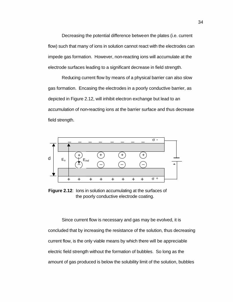
Reducing current flow by means of a physical barrier can also slow

gas formation. Encasing the electrodes in a poorly conductive barrier, as

depicted in Figure 2.12, will inhibit electron exchange but lead to an

accumulation of non-reacting ions at the barrier surface and thus decrease

field strength.

Since current flow is necessary and gas may be evolved, it is

concluded that by increasing the resistance of the solution, thus decreasing

current flow, is the only viable means by which there will be appreciable

electric field strength without the formation of bubbles. So long as the

amount of gas produced is below the solubility limit of the solution, bubbles

Figure 2.12: Ions in solution accumulating at the surfaces of the poorly conductive electrode coating.

_ _ _ _ _ _ _ _ σ -

+ + + +

+ + + + + + + + σ +

_ _ _ _ d

+ Eo

Eind

Eind

Eind

35

will not form. Deionized water is used as the protein solvent for this work

since it has an extremely small number of charge carriers and thus has a

very high resistivity. Non-aqueous solvents can also be considered since

they do not undergo the equivalent of hydrolysis.

36

3. Experimental

3.1 Materials

3.1.1 Proteins

The proteins used in the electric field studies are horse heart

cytochrome c (type VI), human albumin (fraction V1), and human apo-

transferrin. All are purchased from Sigma Chemical Company, Missouri,

USA. Aqueous solutions of 1.0 x 10 -4 g/cm3 of each are prepared by

dissolving the protein in deionized water (pH of 5.5 – 6.0 and conductivity of

1.30 ± 0.05 µS at room temperature) for 30 minutes at 37 °C. Solutions not

used within 8 hours are discarded. Due to the high affinity of protein to

glass surfaces, Teflon vials are used to contain the protein solution before

and during experiments.

Cytochrome c

Cytochrome c is found in the mitochondria of all eukaryotic organisms

and is an essential component of the mitochondrial respiratory chain. It is a

hemoprotein that contains an iron-porphryn complex that functions as an

electron carrier. Cytochrome c, from horse heart, is a small globular protein

consisting of a single polypeptide chain of 104 residues. All cytochrome c

polypeptide chains have a cysteine residue at position 17 that serves to link

the heme prosthetic group to the protein. This protein has a molecular

weight of ≈ 12,370 and is soluble in water up to 2.0 x 10 -1 g/cm3. The

isoelectric point is approximately 10 and the redox potential is +0.251 volts

37

[27]. The conductivity of prepared aqueous solutions, determined

experimentally is 7.2 ± 0.4 µS at 25 °C.

Albumin

Serum albumin is a blood protein whose main biological function is to

regulate osmotic pressure of blood. Human albumin has 584 amino acid

residues. Albumin is water-soluble and has a molecular weight of ≈ 66,300

and an isoelectric point of 4.7. The solubility of albumin in water is 5.0 x 10 -

2 g/cm3 [27]. The conductivity of prepared aqueous solutions is

experimentally determined to be 3.8 ± 0.3 µS at 25 °C.

Apo-Transferrin

Human transferrin is a glycoprotein found in human serum. It is a

non-heme iron transport protein (that facilitates the transport of iron to cells).

The iron poor form, apo-transferrin, combines with an iron ion to become

halo-transferrin, the iron saturated form. Apo-transferrin is water soluble, up

to 2.0 x 10 –2 g/cm3, and has a molecular weight of ≈ 78,500 [27]. The

isoelectric point is 5.5 [28] and the conductivity of prepared aqueous

solutions, determined experimentally, is 3.9 ± 0.4 µS at 25 °C.

3.1.2 Deionized Water

Deionized water with a conductivity of 1.30 ± 0.05 µS and a pH of

5.5 - 6.0 at 25 °C is used as the protein solvent in this work.

38

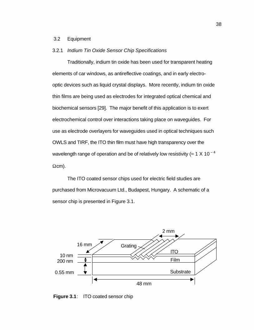
3.2 Equipment

3.2.1 Indium Tin Oxide Sensor Chip Specifications

Traditionally, indium tin oxide has been used for transparent heating

elements of car windows, as antireflective coatings, and in early electro-

optic devices such as liquid crystal displays. More recently, indium tin oxide

thin films are being used as electrodes for integrated optical chemical and

biochemical sensors [29]. The major benefit of this application is to exert

electrochemical control over interactions taking place on waveguides. For

use as electrode overlayers for waveguides used in optical techniques such

OWLS and TIRF, the ITO thin film must have high transparency over the

wavelength range of operation and be of relatively low resistivity (≈ 1 X 10 – 4

Ωcm).

The ITO coated sensor chips used for electric field studies are

purchased from Microvacuum Ltd., Budapest, Hungary. A schematic of a

sensor chip is presented in Figure 3.1.

16 mm

48 mm

2 mm

0.55 mm

∼ 200 nm 10 nm

Substrate

Film

ITO Grating

Figure 3.1: ITO coated sensor chip

39

The sensor chips are ASI type-2400 (Artificial Sensing Instruments, Zurich),

coated with a thin ITO film. Specification for the ASI type 2400 sensor chip

and ITO film are given in Tables 3.1 and 3.2.

Table 3.1: ASI 2400 Sensor Chip Specifications.

ASI Type 2400 Sensor Chips

• Waveguide film Material Si(1-x)TixO2 x=0.25 ± 0.05 Refractive Index (25 °C) nf 1.77 ± 0.03 Thickness df 170 – 220 nm

• Substrate Material Glass (SiO2) Refractive Index (25 °C) ns 1.52578 Thickness ds 0.55 mm

• Diffraction Grating Relief Structure Surface of film Grating Periodicity 2400 lines/mm 0.4166 µm Diffraction Order 1

Grating Dimensions Depth 20 nm Length 2 mm Width 16 mm Grating Line Direction Parallel to width of sensor chip

• Sensor Chip Dimensions Length 48 mm Width 16 mm

40

Table 3.2: ITO Coating Specifications.

ITO Coating

Coating Location Surface of waveguide film Refractive Index (25 °C) nITO ∼ 1.78 Thickness dITO ∼ 10 nm Linear Resistance ∼ 2.08 x 104 Ω/m

3.2.2 Sensor Chip Preparation

Both new and used ITO coated sensor chips are cleaned using the

following procedure. The sensor chip is placed in an ultrasonic bath (of

frequency of 55 kHz), containing a cleaning solution, for 10 minutes and

then is extensively rinsed with deionized water. A cleaning solution at a

concentration of 1.0 x 10 - 2

g/cm3 is prepared by dissolving Terg-A-Zyme

from Alconox (a laboratory detergent with protease) in deionized water. The

effect of the cleaning procedure on the properties of the ITO coated sensor

chip has not yet been determined. However, an analysis of the ASI (Type

2400) sensor chip indicates that the cleaning procedure may affect film

thickness. The analysis of the cleaning procedure is presented in Appendix

B.

Sensor chips are soaked in deionized water (the protein solvent for

this work) for several hours prior to use. Due to the porosity of the

waveguiding film [22, 30], it is found experimentally (and confirmed by

41

literature) that effective refractive index measurements will vary until an

equilibrium condition is reached. Experimental data is presented in

Appendix B.

3.2.3 Optical Biosensor

An integrated optical biosensor, BIOS-1 (Artificial Sensing

Instruments, Zurich, Switzerland) is used to perform all OWLS experiments

[21-25, 31]. The biosensor uses sensor chips, which are comprised of a

glass substrate coated with a thin optically transparent metal oxide film. At

the center of the chip, a relief grating embossed onto the film surface acts to

couple laser light into the film through diffraction. The sample to be

investigated is brought in contact with the film at the grating region by

means of a flow through cuvette.

Measurements are performed and recorded by the biosensor’s

integrated optics scanner, IOS-1. The main components of the scanner are

a He-Ne laser, a mirror (M), the measuring head (MH), a turntable (T) in

which a lever arm (LA) is fixed, a stepper motor (SM), a micrometer screw

(MS) and an optical encoder (E). A schematic of the scanner is presented in

Figure 3.2.

The aluminum-measuring head (MH) of the biosensor’s integrated

optics scanner supports the sensor chip/flow cell apparatus. A photodiode

(D) and a digital potentiometer are located at each end of the measuring

42

head. The sensor chip is mounted into the measuring head such that the

two end faces of the chip, along its width, are aligned with the photodiodes.

Polarized light form a He-Ne laser is directed by a mirror (M) onto the sensor

chip. The measuring head, which is fixed to a turntable (T), is rotated

relative to the fixed beam so that the center of rotation (P1) goes through the

grating region of the sensor chip. A micrometer screw (MS), driven by the

Figure 3.2: Main components of the scanner, IOS-1: He-Ne laser, (M) mirror, (MH) measuring head, (T) turntable, (LA) lever arm, (SM) stepper motor, (MS) micrometer screw, and (E) optical encoder. P1 is the center of rotation, P2 is the engagement point, and XMS is the measured position of the engagement point from XMS=0.

X MS = 0 X MS

Laser

E SM

M

MS

D D

MH

LA

P2

T

P1

43

stepper motor (SM) actuates the lever arm (LA), which is attached to the

turntable (T). An optical encoder (E) measures the position of the stepper

motor. The micrometer screw will contact the lever arm at point (P2) and

from the given distance between P1 and P2, and the measured the position

(XMS) of P2 (from XMS=0), the angular position of the turntable is calculated.

The integrated optics scanner, IOS-1, scans an angular width of up to ± 12.6

degrees. During an angular scan, the photodiodes (D) measure the

intensity of light coupled out of the end faces of the sensor chip. A computer

records the angular peak position of light power as a function of the incident

angle of the laser beam onto the chip (i.e. the angular position of the

turntable).

The incident angle of the laser beam onto the sensor chip at which

light is maximally coupled into the waveguiding film are the basic physical

values determined by the instrument. As protein adsorbs onto the film

surface of the sensor chip, the angles change due to the formation of the

protein adlayer. A computer tracks the values of the incoupling angles with

time.

3.2.4 Flow Cell

The flow cell of the biosensor allows liquid to be brought in contact

with the film surface of a sensor chip at the grating region. The flow cell is

sealed to the surface of the sensor chip with a (n-buna) gasket to create a

flow cavity of volume 7.0 x 10 –2 cm3. Fluid is drawn into the cavity via a

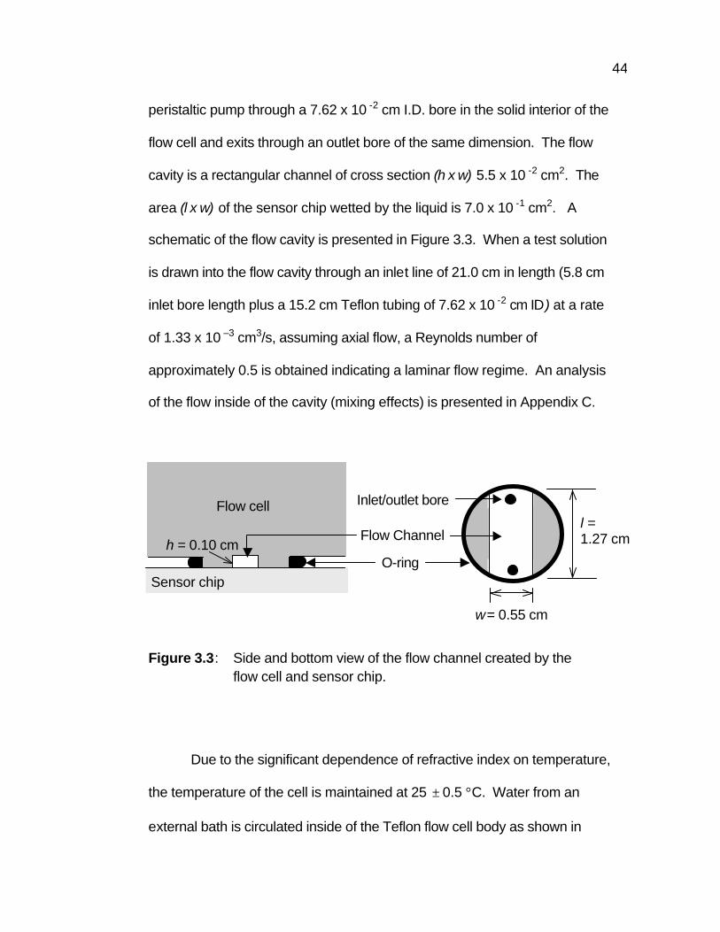
44

peristaltic pump through a 7.62 x 10 -2 cm I.D. bore in the solid interior of the

flow cell and exits through an outlet bore of the same dimension. The flow

cavity is a rectangular channel of cross section (h x w) 5.5 x 10 -2 cm2. The

area (l x w) of the sensor chip wetted by the liquid is 7.0 x 10 -1 cm2. A

schematic of the flow cavity is presented in Figure 3.3. When a test solution

is drawn into the flow cavity through an inlet line of 21.0 cm in length (5.8 cm

inlet bore length plus a 15.2 cm Teflon tubing of 7.62 x 10 -2 cm ID) at a rate

of 1.33 x 10 –3 cm3/s, assuming axial flow, a Reynolds number of

approximately 0.5 is obtained indicating a laminar flow regime. An analysis

of the flow inside of the cavity (mixing effects) is presented in Appendix C.

Due to the significant dependence of refractive index on temperature,

the temperature of the cell is maintained at 25 ± 0.5 °C. Water from an

external bath is circulated inside of the Teflon flow cell body as shown in

Figure 3.3: Side and bottom view of the flow channel created by the flow cell and sensor chip.

O-ring

Flow cell

Sensor chip

Flow Channel

Inlet/outlet bore

w = 0.55 cm

l = 1.27 cm h = 0.10 cm

45

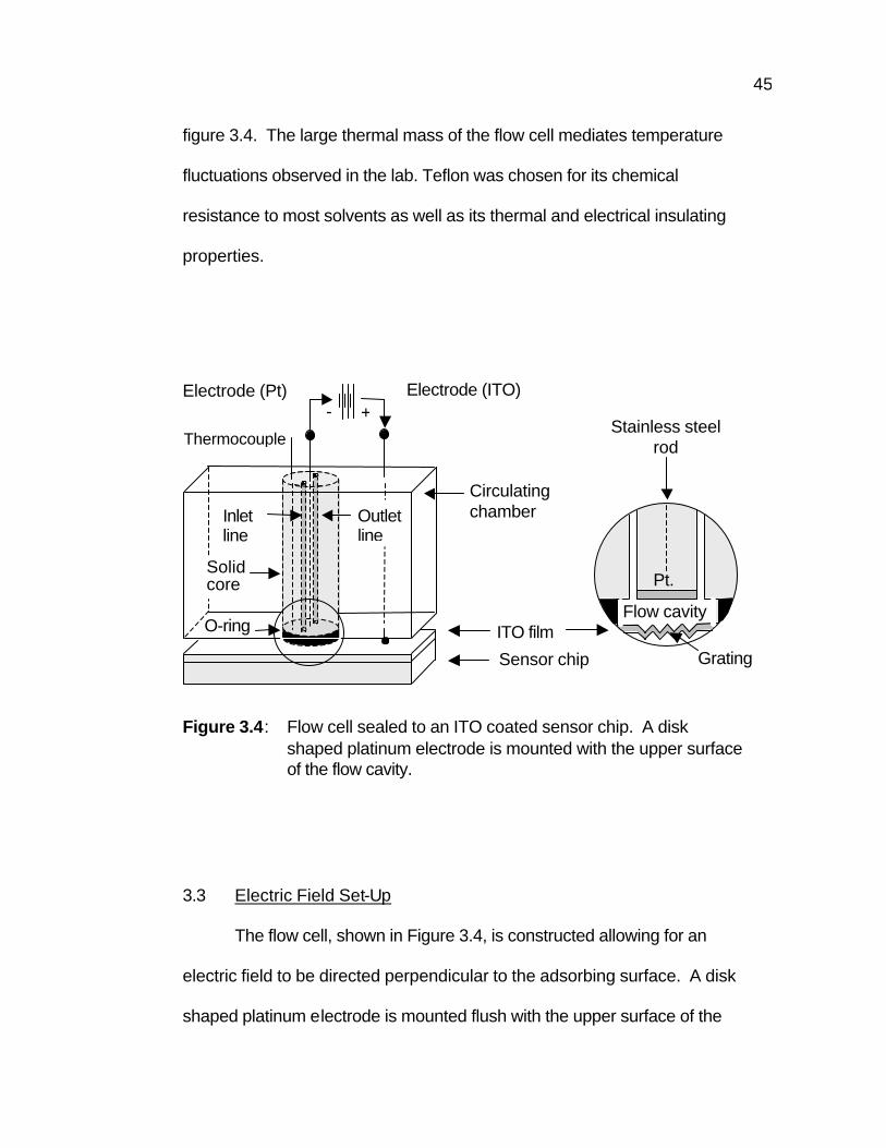
figure 3.4. The large thermal mass of the flow cell mediates temperature

fluctuations observed in the lab. Teflon was chosen for its chemical

resistance to most solvents as well as its thermal and electrical insulating

properties.

3.3 Electric Field Set-Up

The flow cell, shown in Figure 3.4, is constructed allowing for an

electric field to be directed perpendicular to the adsorbing surface. A disk

shaped platinum electrode is mounted flush with the upper surface of the

Figure 3.4: Flow cell sealed to an ITO coated sensor chip. A disk shaped platinum electrode is mounted with the upper surface of the flow cavity.

+-

Sensor chip

Inlet line

Circulating chamber

Electrode (ITO)

ITO film

Electrode (Pt)

Thermocouple

Outlet line

O-ring

Solid core

Stainless steel rod

Flow cavity

Pt.

Grating

46

flow cavity at a distance of 1.0 x 10 -1 cm above the surface of the sensor

chip. The ITO coating (protein adsorbing surface) of a sensor chip acts as

the second electrode in the parallel plate set-up. Electrical contact is made

with the ITO coating through the end of a small steel rod pressed against the

ITO film. Contact is made outside of the flow cavity at a distance of 1.5 cm

from the center of the sensor chip.

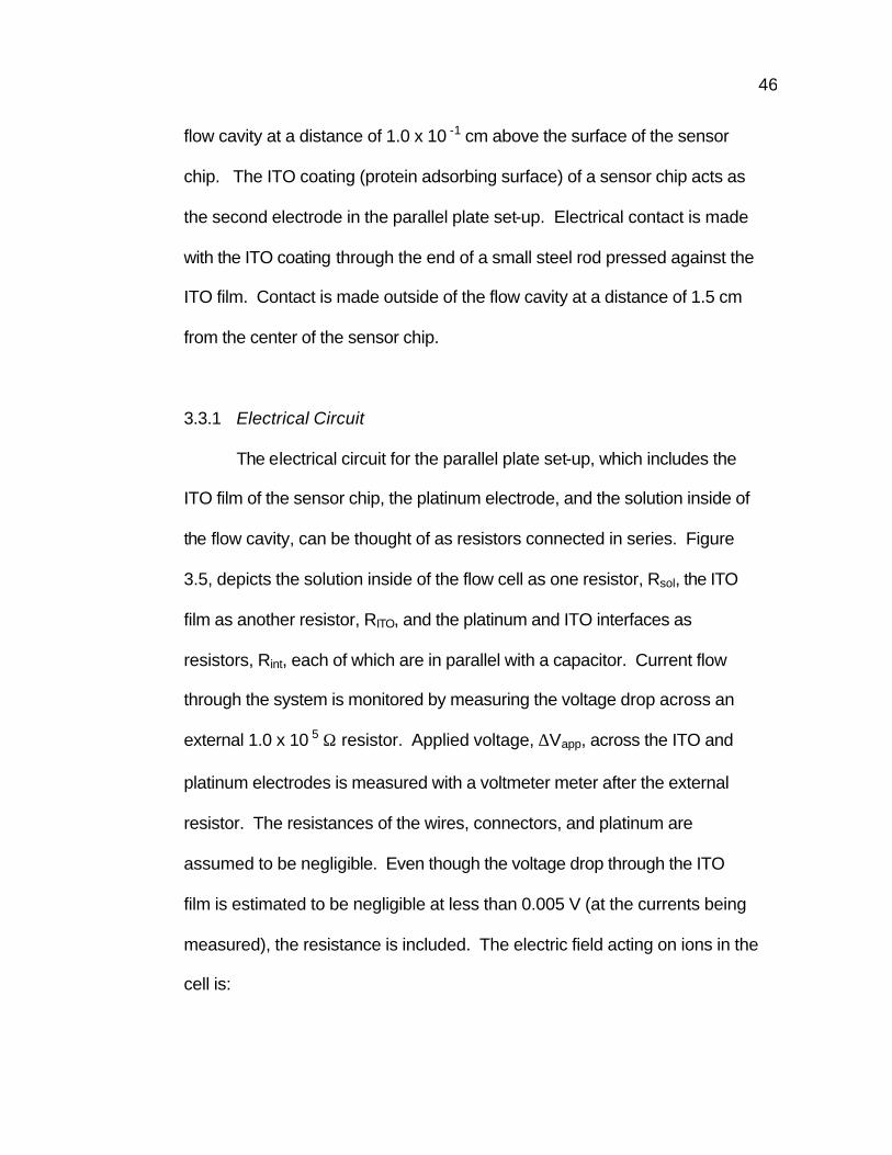
3.3.1 Electrical Circuit

The electrical circuit for the parallel plate set-up, which includes the

ITO film of the sensor chip, the platinum electrode, and the solution inside of

the flow cavity, can be thought of as resistors connected in series. Figure

3.5, depicts the solution inside of the flow cell as one resistor, Rsol, the ITO

film as another resistor, RITO, and the platinum and ITO interfaces as

resistors, Rint, each of which are in parallel with a capacitor. Current flow

through the system is monitored by measuring the voltage drop across an

external 1.0 x 10 5 Ω resistor. Applied voltage, ∆Vapp, across the ITO and

platinum electrodes is measured with a voltmeter meter after the external

resistor. The resistances of the wires, connectors, and platinum are

assumed to be negligible. Even though the voltage drop through the ITO

film is estimated to be negligible at less than 0.005 V (at the currents being

measured), the resistance is included. The electric field acting on ions in the

cell is:

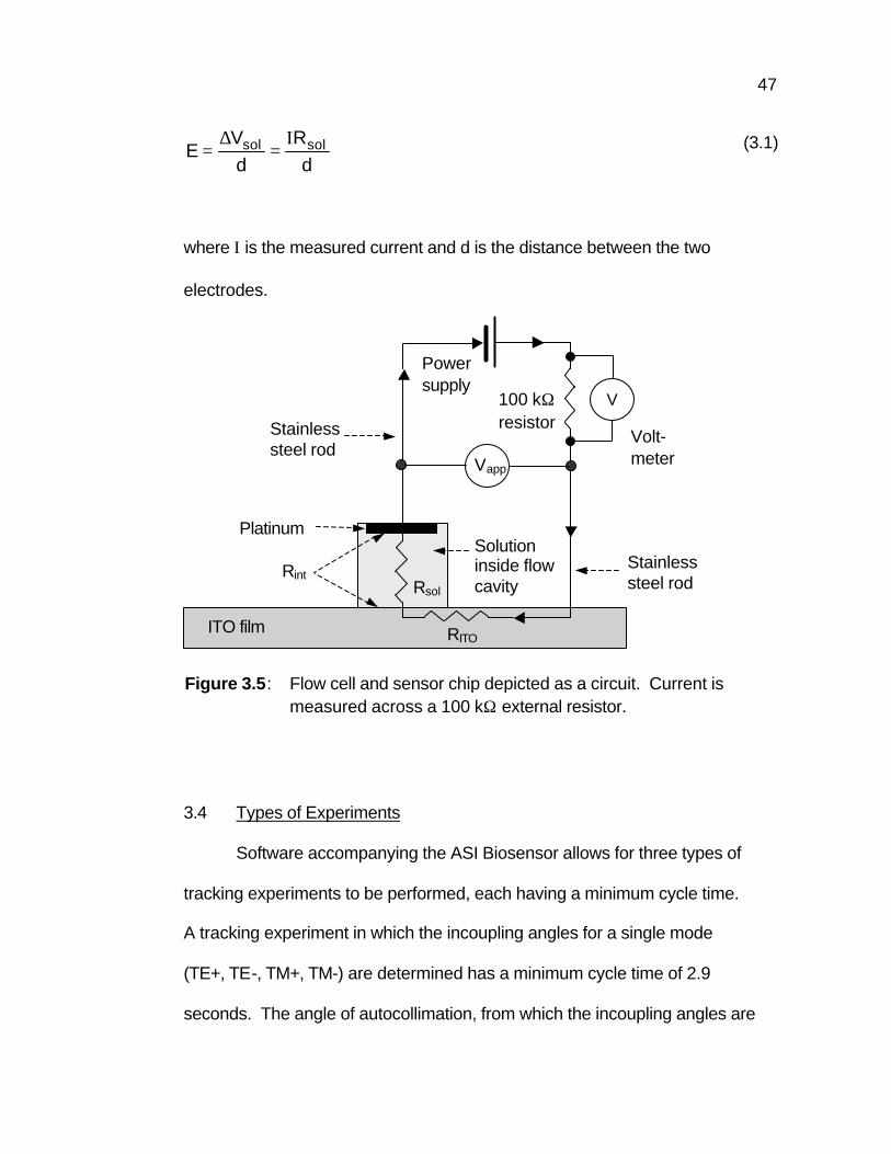
47

dR

dV

E solsol Ι=

∆=

where Ι is the measured current and d is the distance between the two

electrodes.

3.4 Types of Experiments

Software accompanying the ASI Biosensor allows for three types of

tracking experiments to be performed, each having a minimum cycle time.

A tracking experiment in which the incoupling angles for a single mode

(TE+, TE-, TM+, TM-) are determined has a minimum cycle time of 2.9

seconds. The angle of autocollimation, from which the incoupling angles are

Figure 3.5: Flow cell and sensor chip depicted as a circuit. Current is measured across a 100 kΩ external resistor.

(3.1)

Volt- meter

V

Power supply

100 kΩ resistor

ITO film

Platinum

Stainless steel rod

Stainless steel rod

Solution inside flow cavity Rsol

RITO

Vapp

Rint

48

determined, is measured once at the beginning of the experiment. This is

not as accurate as measuring the angle at each scan since drift may occur

during an experiment. To calculate the surface density of protein adsorbed

onto the surface of the sensor chip, equation (2.14) may be used. However,

this expression requires a known value of the refractive index of the protein-

adsorbed layer. This type of experiment has the lowest cycle time and can

be useful when looking at trends involving short-time kinetics.

When performing a two mode or four mode tracking experiment, the

surface density of adsorbed protein can be determined with equation (2.13)

with calculated values of the refractive index and thickness of the protein-

adsorbed layer (from equation 2.11). A two mode (TE+ and TM+) or (TE-

and TM-) tracking experiment has a minimum cycle time of 13.7 seconds

with the angle of autocollimation being measured once, at the beginning of

the experiment. A four mode tracking experiment (TM ± and TE ± ) which

has a minimum cycle time of 23.5 seconds allows the angle of

autocollimation to be measured at each scan providing an even more

accurate measurement.

3.5 Experimental Procedure

The prepared sensor chip and flow cell is mounted into the

biosensing system. Pure solvent (DI water with no protein) is introduced

through the sensor chip/flow cell assembly at a rate of 1.33 x 10 –3 cm3/s.

The temperature of the external water bath is adjusted to maintain the body

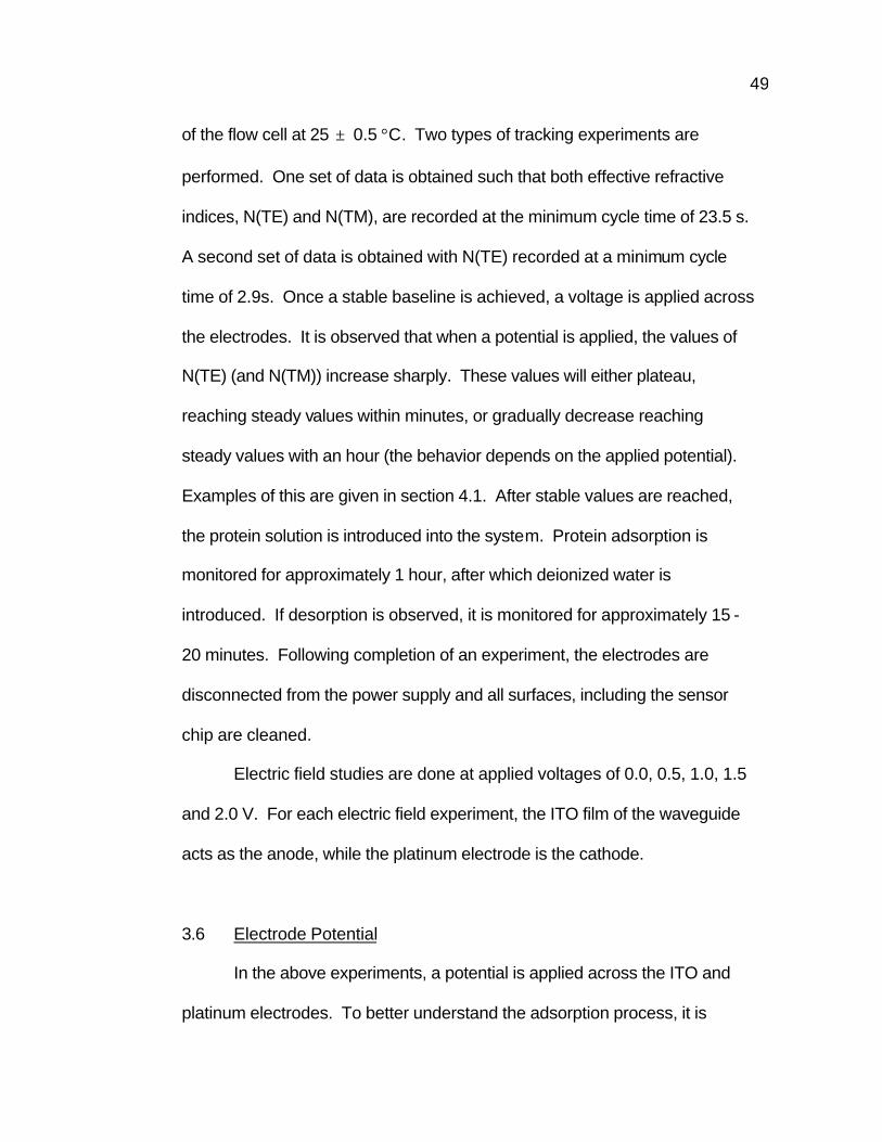
49

of the flow cell at 25 ± 0.5 °C. Two types of tracking experiments are

performed. One set of data is obtained such that both effective refractive

indices, N(TE) and N(TM), are recorded at the minimum cycle time of 23.5 s.

A second set of data is obtained with N(TE) recorded at a minimum cycle

time of 2.9s. Once a stable baseline is achieved, a voltage is applied across

the electrodes. It is observed that when a potential is applied, the values of

N(TE) (and N(TM)) increase sharply. These values will either plateau,

reaching steady values within minutes, or gradually decrease reaching

steady values with an hour (the behavior depends on the applied potential).

Examples of this are given in section 4.1. After stable values are reached,

the protein solution is introduced into the system. Protein adsorption is

monitored for approximately 1 hour, after which deionized water is

introduced. If desorption is observed, it is monitored for approximately 15 -

20 minutes. Following completion of an experiment, the electrodes are

disconnected from the power supply and all surfaces, including the sensor

chip are cleaned.

Electric field studies are done at applied voltages of 0.0, 0.5, 1.0, 1.5

and 2.0 V. For each electric field experiment, the ITO film of the waveguide

acts as the anode, while the platinum electrode is the cathode.

3.6 Electrode Potential

In the above experiments, a potential is applied across the ITO and

platinum electrodes. To better understand the adsorption process, it is

50

desired to know the potential difference across the ITO/solution interface.

However, the potential difference across the interface cannot be measured

directly, but the potential of the ITO electrode relative to a reference

electrode can be measured with a high impedance voltmeter. Electrode

potentials are of interest since they are the governing parameter in

controlling electro-chemical reactions that can occur at the electrode

surface.

The potential of ITO electrode (and that of the platinum) is measured

with an electrometer (model 6514 from Keithley, Ohio, USA) relative to a

saturated gold reference electrode. Theoretically, there should be no

current flow through the reference electrode (current flow is restricted to the

ITO/platinum circuit). However, all potential detection systems are operated

by current. When current is passed through the reference electrode, an

error is induced in the measurement. To minimize this error, a high

impedance (resistance) voltmeter is used.

Potential measurements are done with a gold reference electrode

being placed in the solution reservoir, as shown in figure 3.6. Through the

inlet line leading into the flow cell, the reference electrode is in contact with

the solution near the working electrode (the electrode of interest) inside of

the flow cavity. Two gold reference electrodes, of the same surface area,

are utilized in these measurements. One electrode is placed in a solution

vial that contains deionized water (no protein) and the other is placed in a

reservoir that contains the protein solution. Each of the electrodes is

51

allowed to equalize in their respective solutions for approximately one half

hour before use. The experimental procedure outlined in section 3.5 is

implemented. When switching from water to the protein solution, the

electrometer is disconnected from the reference electrode contained in the

water vial and is reconnected to the reference electrode that is contained in

the protein solution reservoir.

Power supply

Figure 3.6: The potential of the ITO or platinum electrode measured relative to the reference with an electrometer. The external source establishes a current between the electrodes, and its effect on the potential difference of either of them relative to the reference electrode is observed. No current flows through the reference circuit.

Solution reservoir

Solution inside flow cavity

ITO film

EM

Gold reference electrode

Electro-meter Inlet line

Platinum

Reference circuit

Platinum/ITO circuit

52

4. Results and Discussion

4.1 Effect of Electric Field on Instrument Readings

Before examining protein adsorption, it is necessary to determine the

effect of an electric field on instrument readings. To accomplish this, the

refractive index of a glucose solution in both the presence and absence of

an applied field is measured. For each experiment, the flow cavity is initially

filled with deionized water of refractive index 1.33101 ± 1x10 -5 at 25 °C.

Glucose dissolved in deionized water at a concentration 5.0 x 10 -3 g/cm3

and refractive index 1.33173 ± 1x10 -5 at 25 °C (solution indexes

determined with an Abbey refractometer) is allowed to flow through the

channel at a rate of 1.33 x 10 –3 cm3/s. The refractive index of the solution,

at the surface of the sensor chip, versus time is shown in figure 4.1. The

steady state values of the refractive indices for the two experiments

(1.33173 ± 3 x 10 –5 when a potential of 0.0 V is applied and 1.33173 ± 5 x

10 –5 when 5.0 V is applied) are extremely close, indicating that the electric

field does not influence instrument readings. Additionally, the steady state

refractive index values measured at the surface of the sensor chip match

those determined by an Abbey Refractometer (1.33173 ± 1 x 10 –5).

The refractive indices for each of the experimental data sets are

determined with the instrument software. The software uses the mode

equations for planar dielectrics as described with equation (2.11). Since the

ITO film is extremely thin compared to the silicon-titanium dioxide layer, and

its conductivity is relatively low, the two layers are treated as one single film

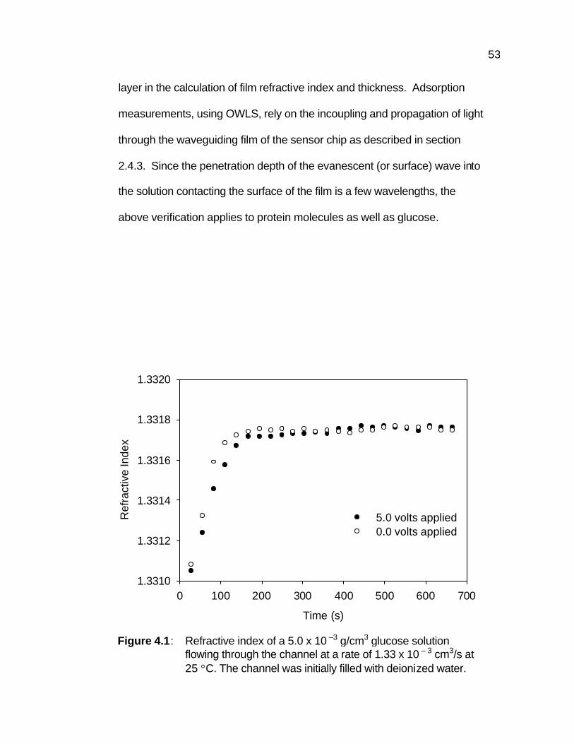
53

layer in the calculation of film refractive index and thickness. Adsorption

measurements, using OWLS, rely on the incoupling and propagation of light

through the waveguiding film of the sensor chip as described in section

2.4.3. Since the penetration depth of the evanescent (or surface) wave into

the solution contacting the surface of the film is a few wavelengths, the

above verification applies to protein molecules as well as glucose.

Figure 4.1: Refractive index of a 5.0 x 10 –3 g/cm3 glucose solution

flowing through the channel at a rate of 1.33 x 10 – 3 cm3/s at 25 °C. The channel was initially filled with deionized water.

Time (s)

0 100 200 300 400 500 600 700

Ref

ract

ive

Inde

x

1.3310

1.3312

1.3314

1.3316

1.3318

1.3320

5.0 volts applied0.0 volts applied

54

4.2 Protein Adsorption: Transport Modes

In general, two distinct kinetic regimes (shown in figure 4.2) can

describe a protein adsorption curve, the transport-limited and adsorption-

limited regimes. In a flow experiment, protein molecules undergo convective

diffusion toward the surface. This is the rate limiting mechanism until a

critical concentration is established near the surface. As adsorption

proceeds, surface availability diminishes thus reducing the rate of

adsorption. When a significant fraction of the surface is covered, the rate of

protein attachment is equal to the rate of detachment and saturation is

reached.

Figure 4.2: Surface density of albumin adsorbed onto an ITO coated sensor chip when a potential of 0.0 V is applied.

Time (s)

0 1000 2000 3000 4000

Sur

face

Den

sity

(µg/

cm2 )

0.00

0.05

0.10

0.15

0.20

0.25

0.30

Adsorption limited region

Transport-limited regime

Approach to saturation

55

By recasting the data presented in figure 4.2 and plotting the

adsorption rate, ∂Γ/∂t, versus the adsorbed amount, Γ, of protein, the

different kinetic regimes are further distinguished. Figure 4.3 shows three

distinct regions: an initial transient transport-limited region, a linear region of

the adsorption-limited regime, and an asymptotic region of the adsorption-

limited regime.

Γ (µg/cm2)

0.00 0.05 0.10 0.15 0.20 0.25 0.30 0.35

dΓdt

(µg/

cm2 /s

)

-0.0002

0.0000

0.0002

0.0004

0.0006

0.0008

0.0010

0.0012

Figure 4.3: Change in surface density with time versus surface density for albumin when a potential of 0.0 V is applied.

Transient transport- limited regime

Adsorption-limited regime (linear region)

Adsorption-limited regime (asymptotic region)

56

A transient region is observed during the very early stage of adsorption

because a stable concentration gradient has not yet been established

(Appendix C). Following sufficient adsorption to the surface, an adsorption-

limited regime is evident, where surface availability is the rate limiting

mechanism. In this regime the rate of adsorption, dΓ/dt, decreases linearly

with increasing surface density, Γ. This linear behavior is predicted by each

adsorption model discussed in section 2.3. When a significant fraction of

the surface covered, a non-linear approach to saturation is observed. In

section 4.3, experimental data for human albumin, cytochrome c, and apo-

transferrin are presented and an analysis of the affect of an applied potential

on the various regions of the adsorption curve is performed.

4.3 Protein Adsorption in an Applied Electric Field

Electric field studies are done at applied potentials of 0.0, 0.5, 1.0,

1.5, and 2.0 volts. For the case of an applied potential of 0.0 V, the two

electrodes are left as an open circuit. For each experiment, the ITO film of

the sensor chip acts as the anode and is the protein-adsorbing surface.

4.3.1 Adsorption Curves

Albumin

In figures 4.4 and 4.5, the adsorbed density versus time for human

albumin onto ITO coated waveguides A and B at applied potentials of 0.0,

0.5, 1.0, 1.5 and 2.0 volts is shown. At an applied potential of 0.0 V, the

57

adsorption curves plateau and saturation is reached within the time scale of

the experiment. At larger applied potentials, the adsorption curves no

longer reach saturation and the total amount of protein on each waveguide

is seen to increase with increasing applied voltage. It is also observed,

during the later stage of adsorption (t ≥ 1800 s), the slope of each

adsorption curve increases with increasing potential (i.e. the slopes rank

with applied voltage).

Albumin (Waveguide A)

Time (s)

0 1000 2000 3000 4000

Sur

face

Den

sity

(µg/

cm2 )

0.0

0.2

0.4

0.6

0.8

1.0

1.2

1.4

2.0 volts applied


1.5 volts applied

0.0 volts applied

Figure 4.4: Surface density of albumin adsorbed onto waveguide A. Data is obtained (every 23.5 s) at 25 °C, at a flow rate of 1.33 x 10 –3 cm3/s.

58

Even though the trends mentioned above are similar for the adsorption of

albumin onto waveguides A and B, the absolute values of the surface

density differ. The variability between runs (less than 30%) is most likely

due to differences in the surface quality of each senor chip. From Appendix

B, it is observed that multiple runs on the same sensor chip yield far less

variability between runs.

Figure 4.5: Surface density of albumin adsorbed onto waveguide B. Data is obtained (every 2.9 s) at 25 °C, at a flow rate of 1.33 x 10 –3 cm3/s.

Albumin (Waveguide B)

Time (s)

0 1000 2000 3000 4000

Sur

face

Den

sity

(µg

/cm

2 )

0.0

0.2

0.4

0.6

0.8

1.0

1.2

1.4

1.6

2.0 volts applied

1.5 volts applied

1.0 volts applied

0.5 volts applied

0.0 volts applied

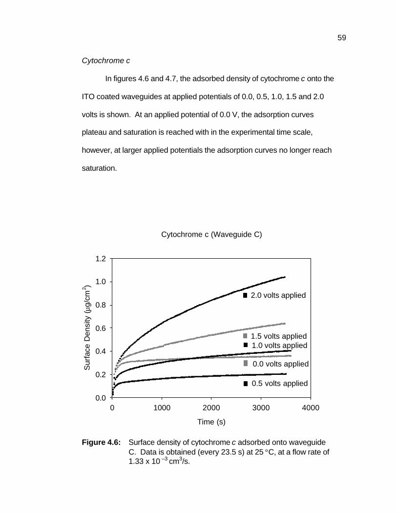
59

Cytochrome c

In figures 4.6 and 4.7, the adsorbed density of cytochrome c onto the

ITO coated waveguides at applied potentials of 0.0, 0.5, 1.0, 1.5 and 2.0

volts is shown. At an applied potential of 0.0 V, the adsorption curves

plateau and saturation is reached with in the experimental time scale,

however, at larger applied potentials the adsorption curves no longer reach

saturation.

Figure 4.6: Surface density of cytochrome c adsorbed onto waveguide C. Data is obtained (every 23.5 s) at 25 °C, at a flow rate of 1.33 x 10 –3 cm3/s.

Cytochrome c (Waveguide C)

Time (s)

0 1000 2000 3000 4000

Sur

face

Den

sity

(µg/

cm2 )

0.0

0.2

0.4

0.6

0.8

1.0

1.2

2.0 volts applied


0.5 volts applied

0.0 volts applied

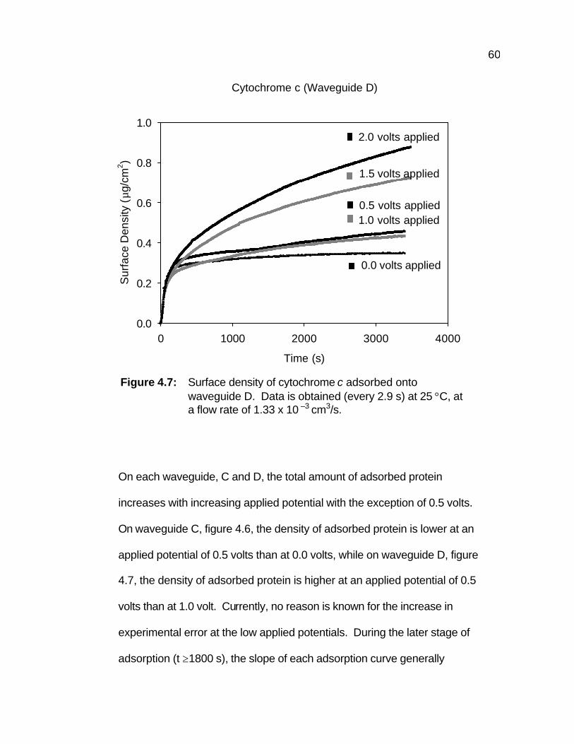
60

On each waveguide, C and D, the total amount of adsorbed protein

increases with increasing applied potential with the exception of 0.5 volts.

On waveguide C, figure 4.6, the density of adsorbed protein is lower at an

applied potential of 0.5 volts than at 0.0 volts, while on waveguide D, figure

4.7, the density of adsorbed protein is higher at an applied potential of 0.5

volts than at 1.0 volt. Currently, no reason is known for the increase in

experimental error at the low applied potentials. During the later stage of

adsorption (t ≥1800 s), the slope of each adsorption curve generally

Figure 4.7: Surface density of cytochrome c adsorbed onto waveguide D. Data is obtained (every 2.9 s) at 25 °C, at a flow rate of 1.33 x 10 –3 cm3/s.

Cytochrome c (Waveguide D)

Time (s)

0 1000 2000 3000 4000

Sur

face

Den

sity

(µg

/cm

2 )

0.0

0.2

0.4

0.6

0.8

1.02.0 volts applied

1.5 volts applied


0.0 volts applied

61

increases with increasing potential. As discussed previously, variations

between runs are expected when comparing data generated on two

separate sensor chips. However, at an applied potential of 0.5 V, the

variation between runs on waveguides C and D exceeds that what is

normally observed and appears to be specific for the case of cytochrome c.

Apo-Transferrin

In figure 4.8, the adsorbed density of apo-transferrin onto the ITO

coated waveguides at applied potentials of 0.0, 0.5, 1.0, and 2.0 volts is

shown.

Figure 4.8: Surface density of Apo-transferrin adsorbed onto Waveguide E. Data is obtained every 23.5 s.

Apo-Transferrin (Waveguide E)

Time (s)

0 1000 2000 3000 4000

Sur

face

Den

sity

(µg/

cm2 )

0.0

0.2

0.4

0.6

0.8

1.0

0.5 volts applied

1.0 volts applied

0.0 volts applied

2.0 volts applied

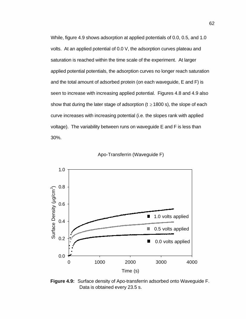
62

While, figure 4.9 shows adsorption at applied potentials of 0.0, 0.5, and 1.0

volts. At an applied potential of 0.0 V, the adsorption curves plateau and

saturation is reached within the time scale of the experiment. At larger

applied potential potentials, the adsorption curves no longer reach saturation

and the total amount of adsorbed protein (on each waveguide, E and F) is

seen to increase with increasing applied potential. Figures 4.8 and 4.9 also

show that during the later stage of adsorption (t ≥ 1800 s), the slope of each

curve increases with increasing potential (i.e. the slopes rank with applied

voltage). The variability between runs on waveguide E and F is less than

30%.

Figure 4.9: Surface density of Apo-transferrin adsorbed onto Waveguide F. Data is obtained every 23.5 s.

Apo-Transferrin (Waveguide F)

Time (s)

0 1000 2000 3000 4000

Sur

face

Den

sity

(µg/

cm2 )

0.0

0.2

0.4

0.6

0.8

1.0

1.0 volts applied

0.5 volts applied

0.0 volts applied

63

4.3.2 Transport-Limited Regime

In the absence of an applied electric field, in a flow experiment,

protein molecules undergo convective diffusion toward the surface. This is

the rate limiting mechanism until a critical concentration is established near

the surface. However, when adsorbing protein in the presence of an applied

electric field, forces resulting from the field act on the molecules. The

electric field forces acting on net negatively charged molecules are in the

vertical direction towards the surface, while those acting on a net positively

charged molecules are in the opposite direction. Any observed increase in

the rate of adsorption in this regime, for the case of negatively charged

proteins, indicates that the electric field forces are sufficient to enhance the

rate above that of concentration driven diffusion alone. Similarly, for

positively charged proteins, any observed decrease in rate would signify that

the electric field forces are sufficient to impede diffusion. When dissolved in

deionized water of pH of 5.5-6.0, albumin is net negatively charged,

cytochrome c is positively charged, and apo-transferrin is close to neutral.

To examine the affect of an applied potential on protein adsorption in

the transient transport-limited regime (as described in section 4.2) the data

presented in section 4.3 is recast. The adsorption rate, ∂Γ/∂t, as a function

of time, t, is plotted for values of t = 0 up to the function’s maximum (i.e. the

maximum value of ∂Γ/∂t). As seen from figure 4.10, the transient transport-

limited regime is described by an increase in the rate with time.

64

Albumin

In figure 4.11, the adsorption rate, ∂Γ/∂t, as a function of time for

albumin adsorbing onto waveguide B is shown. An increase in rate with

increasing applied potential is generally observed. This trend is seen for

adsorption on both waveguides A and B. From figure 4.11, the adsorption

curve obtained at an applied potential of 0.0 V show a difference in slope

when compared to those obtained at higher potentials. However, since the

adsorption data obtained for waveguide A is taken at 23.5 s intervals, there

are an insufficient number of data points to compare the slopes in this region

Figure 4.10: ∂Γ/∂t, as a function of time for albumin adsorbing onto waveguide B at an applied potential of 1.0 V.

Time (s)

0 50 100 150 200 250

dΓdt

(µg/

cm2 /s

)

0.000

0.001

0.002

0.003

0.004Maximum

Transient transport-limited region

Adsorption-limited regime

65

with those obtained for waveguide B (where data is taken at 2.9 s intervals).

Therefore, no inference regarding the slope can be made at this time.


Time (s)

0 50 100 150 200

dΓ/d

t (µg

/cm

2 /s)

0.000

0.001

0.002

0.003

0.004

0.005

0.0062.0 volts applied1.5 volts applied 1.0 volts applied0.5 volts applied0.0 volts applied

Cytochrome c

In figure 4.12, the adsorption rate, ∂Γ/∂t, as a function time for

cytochrome c adsorbing onto waveguide D is shown. It is observed that the

initial adsorption kinetics is not greatly altered by an applied potential. This

Figure 4.11: Adsorption rate, ∂Γ/∂t, as a function time for albumin adsorbing onto waveguide B at applied potentials of 0.0, 0.5, 1.0, 1.5, and 2.0 V.

66

trend is seen for adsorption on both waveguides C and D. This result differs

from that of albumin, which shows an increase in the rate of adsorption with

increasing applied potential. From figure 4.12, the adsorption curves show

slight differences in slope. However, since the adsorption data obtained for

waveguide C is taken at 23.5 s intervals, there are an insufficient number of

data points to compare the slopes in this region with those obtained for

waveguide D (where data is taken at 2.9 s intervals). Therefore, no

inference regarding the slope can be made at this time.


Time (s)

0 20 40 60 80 100

dΓ/d

t (µg

/cm

2 /s)

0.000

0.001

0.002

0.003

0.004

0.005

0.006

2.0 volts applied1.5 volts applied1.0 volts applied0.5 volts applied0.0 volts applied

Figure 4.12: Adsorption rate, ∂Γ/∂t, as a function time for cytochrome c adsorbing onto waveguide D at applied potentials of 0.0, 0.5, 1.0, 1.5, and 2.0 V.

67

Apo-Transferrin

In figure 4.13, the adsorption rate, ∂Γ/∂t, as a function time for

transferrin adsorbing onto waveguide E is shown. It is observed that the

initial adsorption kinetics is not greatly altered by an applied potential.

Since the adsorption data obtained for waveguides E and F are taken at

23.5 s intervals, there are an insufficient number of data points generate

slopes in this region. Therefore, no inference regarding the slope can be

made at this time.


Time (s)

0 50 100 150 200

dΓ/d

t (µg

/cm

2 /s)

0.000

0.001

0.002

0.003

0.004

0.005

2.0 volts applied1.0 volts applied0.5 volts applied0.0 volts applied

Figure 4.13: Adsorption rate, ∂Γ/∂t, as a function time for apo-transferrin adsorbing onto waveguide E at applied potentials of 0.0, 0.5, 1.0, and 2.0 V.

68

4.3.3 Linear Region of the Adsorption-Limited Regime

As discussed in section 4.3.2, during the very early stage of

adsorption, transport to the surface is the rate-limiting mechanism, which is

characterized by a continuous increase in the rate of adsorption. However,

when surface availability dominates, a decrease in rate is observed. From

plots of adsorption rate, ∂Γ/∂t, as a function of the adsorbed amount, Γ, of

protein, as presented in section 4.2, a linear decrease in the rate with

increasing surface coverage is evident.

Figure 4.14: Change in surface density of adsorbed protein with time versus

density. Apparent initial adsorption rate, ka (cm/s), is determined from the intercept of a line through the linear region of the adsorption-limited regime.

Γ (µg/cm2)

0.0 0.1 0.2 0.3 0.4 0.5 0.6

dΓ/d

t (µg

/cm

2 /s)

0.000

0.001

0.002

0.003

0.004

0.005kac

Transient transport – limited regime

Adsorption-limited regime (asymptotic region)

Adsorption-limited regime (linear region)

69

To examine the effect of an applied potential on adsorption in the

linear region of the adsorption-limited regime, an apparent initial adsorption

rate constant, ka, is determined. The apparent initial adsorption rate

constant is found by fitting a line, as predicted by Langmuir and other

models, to the linear region of the adsorption-limited regime (as shown in

figure 4.14) and extrapolating it to Γ = 0, where the intercept is kac and c is

the bulk concentration of protein [17].

Albumin

Figure 4.15: Change in surface density of adsorbed protein with time versus density for albumin onto waveguide B.


Γ (µg/cm2)

0.0 0.2 0.4 0.6 0.8 1.0 1.2 1.4 1.6

d Γ/d

t (µg

/cm

2 /s)

-0.001

0.000

0.001

0.002

0.003

0.004

0.005

0.006

2.0 volts applied1.5 volts applied1.0 volts applied0.5 volts applied0.0 volts applied

70

In figure 4.15, the adsorption rate, ∂Γ/∂t, as a function of the adsorbed

amount, Γ, of albumin onto waveguide B is shown. The apparent initial

adsorption rate constants, determined by the method previously described,

are seen to increase with increasing applied potential (the for the

experiments conducted on waveguides A and B are presented in table 4.1).

Cytochrome c

In figure 4.16, the adsorption rate, ∂Γ/∂t, as a function of the adsorbed

amount, Γ, of cytochrome c onto waveguide D is shown.

Figure 4.16: Change in surface density of adsorbed protein with time

versus density for cytochrome c onto waveguide D.


Γ (µg/cm2)

0.0 0.2 0.4 0.6 0.8 1.0

d Γ/d

t (µg

/cm

2 /s)

-0.001

0.000

0.001

0.002

0.003

0.004

0.005

0.006


71

The apparent initial adsorption rate constants are not greatly altered by an

applied potential. This result differs from that of albumin, which shows an

increase in the rate constants with increasing applied potential. The values

of the apparent initial adsorption rate constants for the experiments

conducted on waveguides C and D are presented are table 4.1.

Apo-Transferrin

In figure 4.17, the adsorption rate, ∂Γ/∂t, as a function of the

adsorbed amount, Γ, of apo-transferrin on waveguide E is shown.

Figure 4.17: Change in surface density with time versus surface density for

apo-transferrin adsorbed onto waveguide E.


Γ (µg/cm2)

0.0 0.2 0.4 0.6 0.8 1.0

d Γ/d

t (µg

/cm

2 /s)

-0.001

0.000

0.001

0.002

0.003

0.004

0.005

0.006


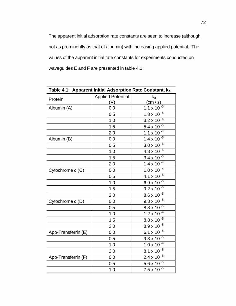
72

The apparent initial adsorption rate constants are seen to increase (although

not as prominently as that of albumin) with increasing applied potential. The

values of the apparent initial rate constants for experiments conducted on

waveguides E and F are presented in table 4.1.

Table 4.1: Apparent Initial Adsorption Rate Constant, ka

Protein Applied Potential (V)

ka (cm / s)

Albumin (A) 0.0 1.1 x 10 -5 0.5 1.8 x 10 -5 1.0 3.2 x 10 -5 1.5 5.4 x 10 -5 2.0 1.1 x 10 -4 Albumin (B) 0.0 1.4 x 10 -5 0.5 3.0 x 10 -5 1.0 4.8 x 10 -5 1.5 3.4 x 10 -5 2.0 1.4 x 10 -4 Cytochrome c (C) 0.0 1.0 x 10 -4 0.5 4.1 x 10 -5 1.0 6.9 x 10 -5 1.5 9.2 x 10 -5 2.0 8.6 x 10 -5 Cytochrome c (D) 0.0 9.3 x 10 -5 0.5 8.8 x 10 -5 1.0 1.2 x 10 -4 1.5 8.8 x 10 -5 2.0 8.9 x 10 -5 Apo-Transferrin (E) 0.0 6.1 x 10 -5 0.5 9.3 x 10 -5 1.0 1.0 x 10 -4 2.0 8.1 x 10 -5 Apo-Transferrin (F) 0.0 2.4 x 10 -5 0.5 5.6 x 10 -5 1.0 7.5 x 10 -5

73

4.3.3 Asymptotic Adsorption Rate

To look at the affect of an applied potential on adsorption in the non-

linear asymptotic region of the adsorption–limited regime (as described in

section 4.2), the region of each adsorption curve (presented in section

4.3.1), is fit with the following two expressions for times, t ≥ 1800 s

where Γ(8) is the surface density of adsorbed protein when t? 8, kb is the

asymptotic rate constant and, ν is a time constant. When adsorbing protein

onto a solid surface it is observed experimentally and predicted theoretically,

that at long times, the surface density of protein asymptotically reaches a

steady state where the protein continues to adsorb and desorb. It has been

shown theoretically, by the Simple Particle Model, that an irreversible

approach to saturation is described by power law behavior (equation 4.2).

However, when desorption or surface diffusion is incorporated into the

model, the approach to saturation is described by the exponential function

(equation 4.1).

When examining the experimental data, surface density versus time

obtained for each of the three proteins for t ≥ 1800 s, it is observed that

equations 4.1 and 4.2 described the data equally well in terms of fit.

However, when applying equation 4.2 unrealistic large values of Γ(8) are

(4.1)

(4.2) ν−−∞Γ=Γ

ν−−∞Γ=Γ

tk)()t(

)texp(k)()t(

b

b

74

generated. By calculating the theoretical monolayer coverage, Γmonolayer =

mp / (d1d2), of a protein, (where mp is the mass of a single protein molecule

and d1 and d2 are the dimensions of the protein) and comparing this value to

those of obtained for Γ(8), several inference can be made. An analysis of

the adsorption curve (figure 4.5) for human albumin adsorbing onto

waveguige B at an applied potentials of 2.0 V will serve as an appropriate

example. The theoretical monolayer coverage for albumin is 0.2 µg/cm2,

where mp = 1.1 x 10 –13 µg, d1 = 1.5 x 10 –6 cm, and d2 = 3.8 x 10 –7 cm.

This value of Γmonolayer is in agreement with the saturation values seen with

the experimental results at an applied potential of 0.0 V. When fitting the

adsorption curve for albumin at an applied potential of 2.0 V, the power law

fit of the adsorption curve, for t ≥ 1800, gives a value of Γ(8) = 336.8 µg/cm2

where the exponential equation predicts Γ(8) = 1.7 µg/cm2. Even though

the results obtained with equations 4.1 and 4.2 both predict a surface

coverage that exceed the theoretical monolayer, it can be assumed that a

surface coverage exceeding that of a monolayer by four orders of magnitude

is unreasonable. Since the exponential equation gives realistic values of

Γ(8) that are in good agreement with the experimental data, it is concluded

that the approach to saturation is exponential in nature. For the adsorption

of albumin under applied potentials larger than 0.0 V, the values of Γ(8)

exceed that of the theoretical monolayer coverage. This is most likely due

to the formation of multiple layers, although at this time tighter packing of the

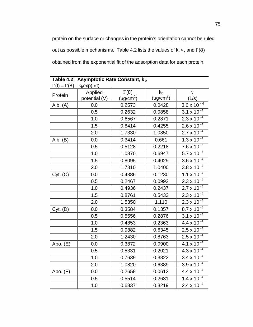
75

protein on the surface or changes in the protein’s orientation cannot be ruled

out as possible mechanisms. Table 4.2 lists the values of k, ν, and Γ(8)

obtained from the exponential fit of the adsorption data for each protein.

Table 4.2: Asymptotic Rate Constant, kb Γ(t) = Γ(8) - kbexp(-νt)

Protein Applied potential (V)

Γ(8) (µg/cm2)

kb (µg/cm2)

ν (1/s)

Alb. (A) 0.0 0.2573 0.0428 3.6 x 10 - 4 0.5 0.2632 0.0858 3.1 x 10 -4

1.0 0.6567 0.2871 2.3 x 10 -4

1.5 0.8414 0.4255 2.6 x 10 -4

2.0 1.7330 1.0850 2.7 x 10 -4

Alb. (B) 0.0 0.3414 0.661 1.3 x 10 -4

0.5 0.5128 0.2218 7.6 x 10 -5

1.0 1.0870 0.6947 5.7 x 10 -5

1.5 0.8095 0.4029 3.6 x 10 -4

2.0 1.7310 1.0400 3.8 x 10 -4

Cyt. (C) 0.0 0.4386 0.1230 1.1 x 10 -4

0.5 0.2467 0.0992 2.3 x 10 -4

1.0 0.4936 0.2437 2.7 x 10 -4

1.5 0.8761 0.5433 2.3 x 10 -4

2.0 1.5350 1.110 2.3 x 10 -4

Cyt. (D) 0.0 0.3584 0.1357 8.7 x 10 -4

0.5 0.5556 0.2876 3.1 x 10 -4

1.0 0.4853 0.2363 4.4 x 10 -4

1.5 0.9882 0.6345 2.5 x 10 -4

2.0 1.2430 0.8763 2.5 x 10 -4

Apo. (E) 0.0 0.3872 0.0900 4.1 x 10 -4

0.5 0.5331 0.2021 4.3 x 10 -4

1.0 0.7639 0.3822 3.4 x 10 -4

2.0 1.0820 0.6389 3.9 x 10 -4

Apo. (F) 0.0 0.2658 0.0612 4.4 x 10 -4

0.5 0.5514 0.2631 1.4 x 10 -4

1.0 0.6837 0.3219 2.4 x 10 -4

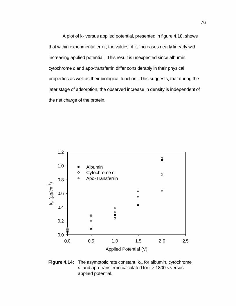
76

A plot of kb versus applied potential, presented in figure 4.18, shows

that within experimental error, the values of kb increases nearly linearly with

increasing applied potential. This result is unexpected since albumin,

cytochrome c and apo-transferrin differ considerably in their physical

properties as well as their biological function. This suggests, that during the

later stage of adsorption, the observed increase in density is independent of

the net charge of the protein.

Applied Potential (V)

0.0 0.5 1.0 1.5 2.0 2.5

k b ( µ

g/cm

2 )

0.0

0.2

0.4

0.6

0.8

1.0

1.2

Albumin Cytochrome cApo-Transferrin

Figure 4.14: The asymptotic rate constant, kb, for albumin, cytochrome

c, and apo-transferrin calculated for t ≥ 1800 s versus applied potential.

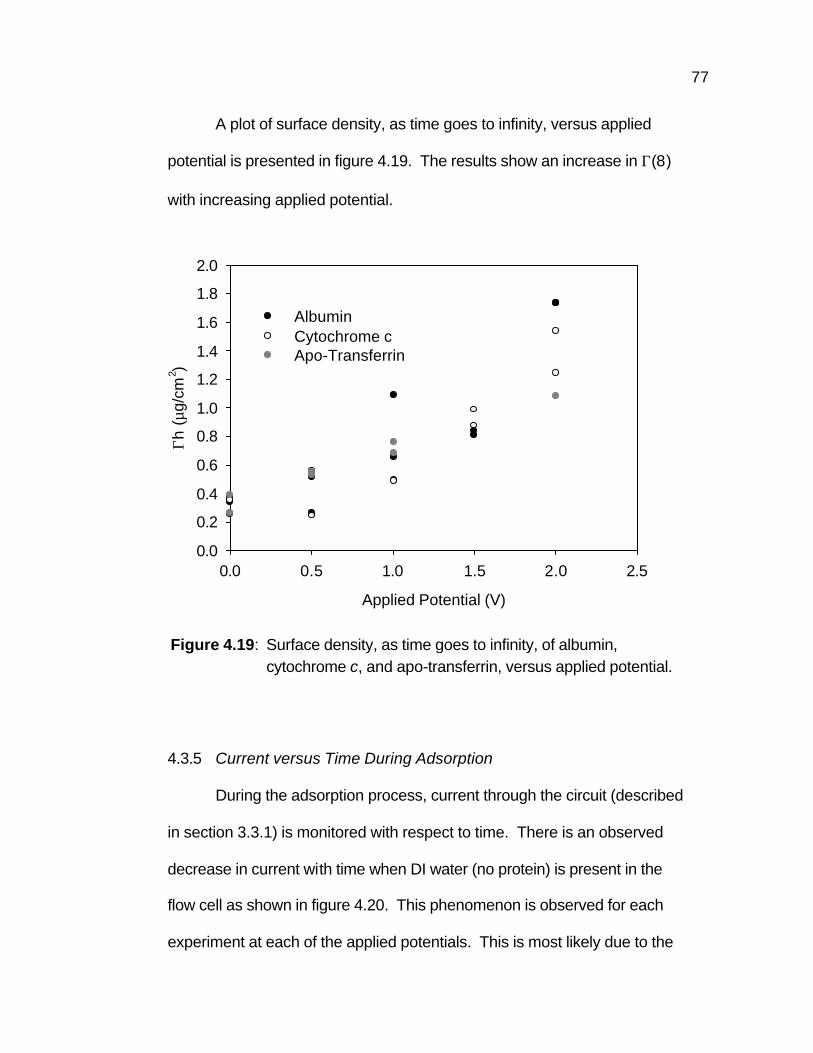
77

A plot of surface density, as time goes to infinity, versus applied

potential is presented in figure 4.19. The results show an increase in Γ(8)

with increasing applied potential.

4.3.5 Current versus Time During Adsorption

During the adsorption process, current through the circuit (described

in section 3.3.1) is monitored with respect to time. There is an observed

decrease in current with time when DI water (no protein) is present in the

flow cell as shown in figure 4.20. This phenomenon is observed for each

experiment at each of the applied potentials. This is most likely due to the

Figure 4.19: Surface density, as time goes to infinity, of albumin, cytochrome c, and apo-transferrin, versus applied potential.

Applied Potential (V)

0.0 0.5 1.0 1.5 2.0 2.5

Γh(µ

g/cm

2 )

0.0

0.2

0.4

0.6

0.8

1.0

1.2

1.4

1.6

1.8

2.0

AlbuminCytochrome cApo-Transferrin

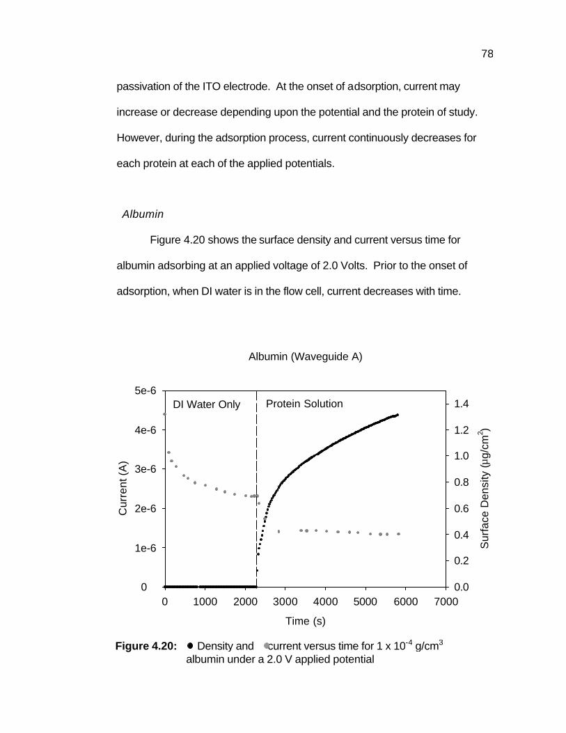
78

passivation of the ITO electrode. At the onset of adsorption, current may

increase or decrease depending upon the potential and the protein of study.

However, during the adsorption process, current continuously decreases for

each protein at each of the applied potentials.

Albumin

Figure 4.20 shows the surface density and current versus time for

albumin adsorbing at an applied voltage of 2.0 Volts. Prior to the onset of

adsorption, when DI water is in the flow cell, current decreases with time.

Albumin (Waveguide A)

Time (s)

0 1000 2000 3000 4000 5000 6000 7000

Sur

face

Den

sity

(µg/

cm2 )

0.0

0.2

0.4

0.6

0.8

1.0

1.2

1.4

Cur

rent

(A)

0

1e-6

2e-6

3e-6

4e-6

5e-6DI Water Only Protein Solution

Figure 4.20: Density and current versus time for 1 x 10-4 g/cm3 albumin under a 2.0 V applied potential

79

At the onset of adsorption, a rapid decrease in current is observed followed

by a gradual decrease. The above effect is also observed at an applied

potential of 1.5 volts. However at applied potentials of 1.0 and 0.5 volts,

there is an increase in current at the onset of adsorption, after which current

continually decreases.

Current, as a function of time, during the adsorption of human

albumin (figures 4.4 and 4.5) at each of the applied potentials is presented

in figure 4.21. On waveguide A, at an applied potential of 2.0 volts, current

rapidly decreases (40%) during the first 600 s of adsorption after which the

decrease is slight (11%).

Figure 4.21: Current as a function of time during the adsorption process of albumin onto waveguides A and B.

Albumin

Time (s)

0 1000 2000 3000 4000

Cur

rent

(A)

0.0

5.0e-7

1.0e-6

1.5e-6

2.0e-6

2.5e-6

2.0 volts applied ( A, B)




80

At an applied potential of 1.5 volts current changes little with time (10%

decreases from the onset of adsorption). However, at applied potentials of

1.0 and 0.5 volts, there is a slight increase in current at the onset of

adsorption (14% during the first 58s and 7% during the first 164s,

respectively), after which current continuously decreases (28% and 19%,

respectively). Original data is presented in Appendix D.

A similar trend is observed for experiments performed on waveguide

B. At an applied potential of 2.0 volts, current decreases rapidly (22%)

during the first 800 s of adsorption after which the decrease in current is

slight (8%). At an applied potential of 1.5 volts the current decreases from

the onset of adsorption is 18%. Again, when 1.0 and 0.5 volts is applied,

current increases (13% during the first 127s and 7% during the first 92s,

respectively) during the initial stage of adsorption, after which it continuously

decreases (49% and 33%, respectively).

Cytochrome c

Figure 4.22 shows surface density and current versus time for

cytochrome c adsorbing at an applied potential of 2.0 volts. Prior to the

onset of adsorption, when water is in the flow cell, current decreases with

time. When the protein solution is injected into the flow cell, current

increases at the onset of adsorption, then continually decreases throughout

the remainder of the experiment. This effect is observed at each of the

applied potentials.

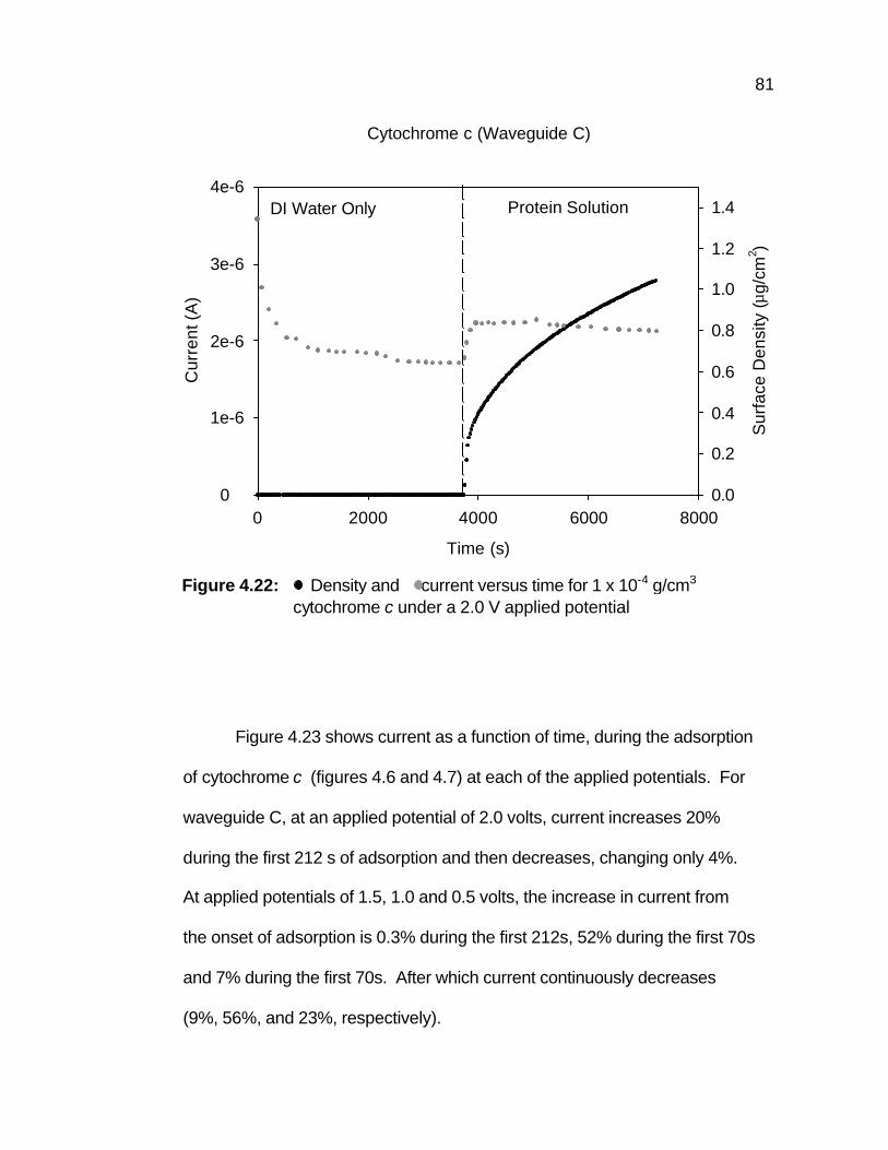
81

Figure 4.23 shows current as a function of time, during the adsorption

of cytochrome c (figures 4.6 and 4.7) at each of the applied potentials. For

waveguide C, at an applied potential of 2.0 volts, current increases 20%

during the first 212 s of adsorption and then decreases, changing only 4%.

At applied potentials of 1.5, 1.0 and 0.5 volts, the increase in current from

the onset of adsorption is 0.3% during the first 212s, 52% during the first 70s

and 7% during the first 70s. After which current continuously decreases

(9%, 56%, and 23%, respectively).

Cytochrome c (Waveguide C)

Time (s)

0 2000 4000 6000 8000

Sur

face

Den

sity

(µg/

cm2 )

0.0

0.2

0.4

0.6

0.8

1.0

1.2

1.4C

urre

nt (A

)

0

1e-6

2e-6

3e-6

4e-6DI Water Only Protein Solution

Figure 4.22: Density and current versus time for 1 x 10-4 g/cm3 cytochrome c under a 2.0 V applied potential

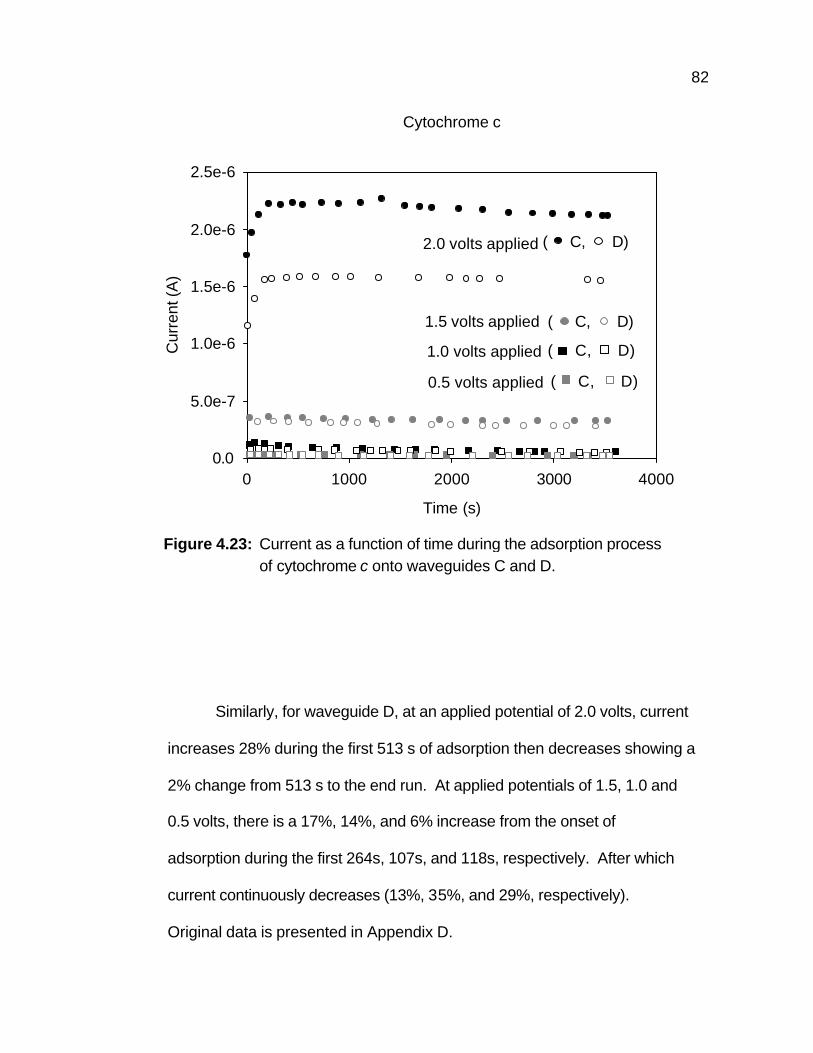
82

Similarly, for waveguide D, at an applied potential of 2.0 volts, current

increases 28% during the first 513 s of adsorption then decreases showing a

2% change from 513 s to the end run. At applied potentials of 1.5, 1.0 and

0.5 volts, there is a 17%, 14%, and 6% increase from the onset of

adsorption during the first 264s, 107s, and 118s, respectively. After which

current continuously decreases (13%, 35%, and 29%, respectively).

Original data is presented in Appendix D.

Figure 4.23: Current as a function of time during the adsorption process of cytochrome c onto waveguides C and D.

Cytochrome c

Time (s)

0 1000 2000 3000 4000

Cur

rent

(A)

0.0

5.0e-7

1.0e-6

1.5e-6

2.0e-6

2.5e-6

2.0 volts applied ( C, D)




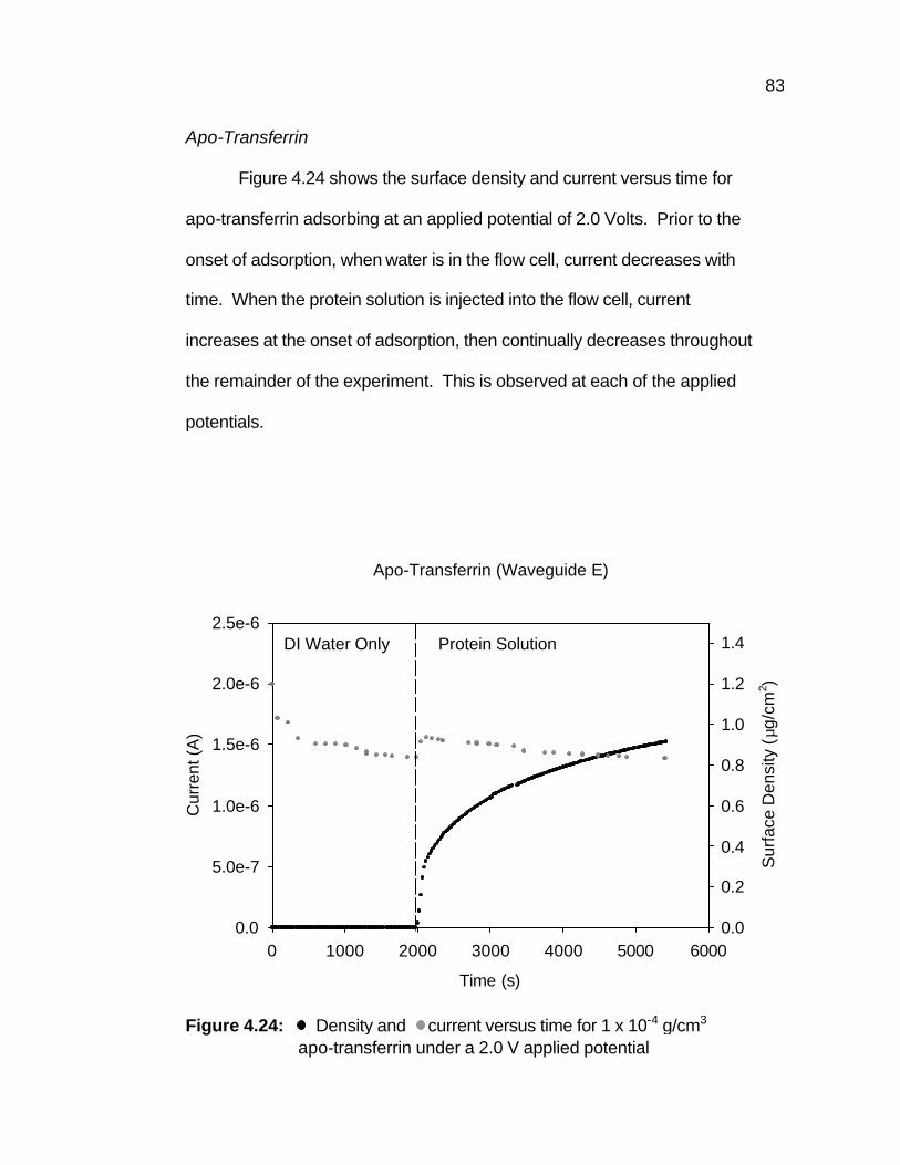
83

Apo-Transferrin

Figure 4.24 shows the surface density and current versus time for

apo-transferrin adsorbing at an applied potential of 2.0 Volts. Prior to the

onset of adsorption, when water is in the flow cell, current decreases with

time. When the protein solution is injected into the flow cell, current

increases at the onset of adsorption, then continually decreases throughout

the remainder of the experiment. This is observed at each of the applied

potentials.


Time (s)

0 1000 2000 3000 4000 5000 6000

Sur

face

Den

sity

(µg

/cm

2 )

0.0

0.2

0.4

0.6

0.8

1.0

1.2

1.4

Cur

rent

(A)

0.0

5.0e-7

1.0e-6

1.5e-6

2.0e-6

2.5e-6DI Water Only Protein Solution

Figure 4.24: Density and current versus time for 1 x 10-4 g/cm3 apo-transferrin under a 2.0 V applied potential

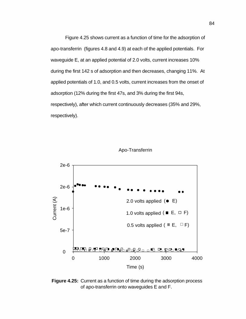
84

Figure 4.25 shows current as a function of time for the adsorption of

apo-transferrin (figures 4.8 and 4.9) at each of the applied potentials. For

waveguide E, at an applied potential of 2.0 volts, current increases 10%

during the first 142 s of adsorption and then decreases, changing 11%. At

applied potentials of 1.0, and 0.5 volts, current increases from the onset of

adsorption (12% during the first 47s, and 3% during the first 94s,

respectively), after which current continuously decreases (35% and 29%,

respectively).

Figure 4.25: Current as a function of time during the adsorption process of apo-transferrin onto waveguides E and F.

Apo-Transferrin

Time (s)

0 1000 2000 3000 4000

Cur

rent

(A)

0

5e-7

1e-6

2e-6

2e-6

1.0 volts applied ( E, F)

2.0 volts applied ( E)

0.5 volts applied ( E, F)

85

For waveguide F, at applied potentials of 1.0, and 0.5 volts, current

increases 11% during the first 117s, and 5% during the first 95s of

adsorption. After which there is a continuous decrease in current, 31%, and

27%, respectively. Original data is presented in Appendix D.

As seen in figures 4.20, 4.22, and 4.24, at the onset of adsorption

current increases with time. This is followed by a steady decrease in current

flow. This phenomenon is observed for each protein at each of the applied

potentials with the exception of human albumin. At the higher applied

potentials (1.5 and 2.0 volts), a decrease in current flow is observed at the

onset of adsorption. This is of note since albumin is the only protein tested

that has a net charge opposite of that of the adsorbing surface and which an

applied potential has an impact on the initial adsorption rate.

4.3.6 Electrode Potentials

In the above experiments, a potential is applied across the ITO (the

protein adsorbing surface) and platinum electrodes. To better understand

the adsorption process, it is desired to know the potential difference across

the ITO/solution interface. However, the potential difference across the

interface cannot be measured directly, but the potential of the ITO electrode

relative to a reference electrode can be measured with a high impedance

voltmeter. Electrode potentials are of interest since they are the governing

parameter in controlling electro-chemical reactions that can occur at the

electrode surface.

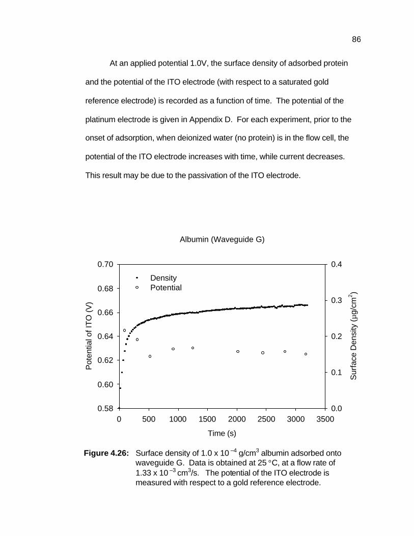
86

At an applied potential 1.0V, the surface density of adsorbed protein

and the potential of the ITO electrode (with respect to a saturated gold

reference electrode) is recorded as a function of time. The potential of the

platinum electrode is given in Appendix D. For each experiment, prior to the

onset of adsorption, when deionized water (no protein) is in the flow cell, the

potential of the ITO electrode increases with time, while current decreases.

This result may be due to the passivation of the ITO electrode.

Albumin (Waveguide G)

Time (s)

0 500 1000 1500 2000 2500 3000 3500

Sur

face

Den

sity

(µg/

cm2 )

0.0

0.1

0.2

0.3

0.4

Pot

entia

l of I

TO

(V

)

0.58

0.60

0.62

0.64

0.66

0.68

0.70

DensityPotential

Figure 4.26: Surface density of 1.0 x 10 –4 g/cm3 albumin adsorbed onto waveguide G. Data is obtained at 25 °C, at a flow rate of 1.33 x 10 –3 cm3/s. The potential of the ITO electrode is measured with respect to a gold reference electrode.

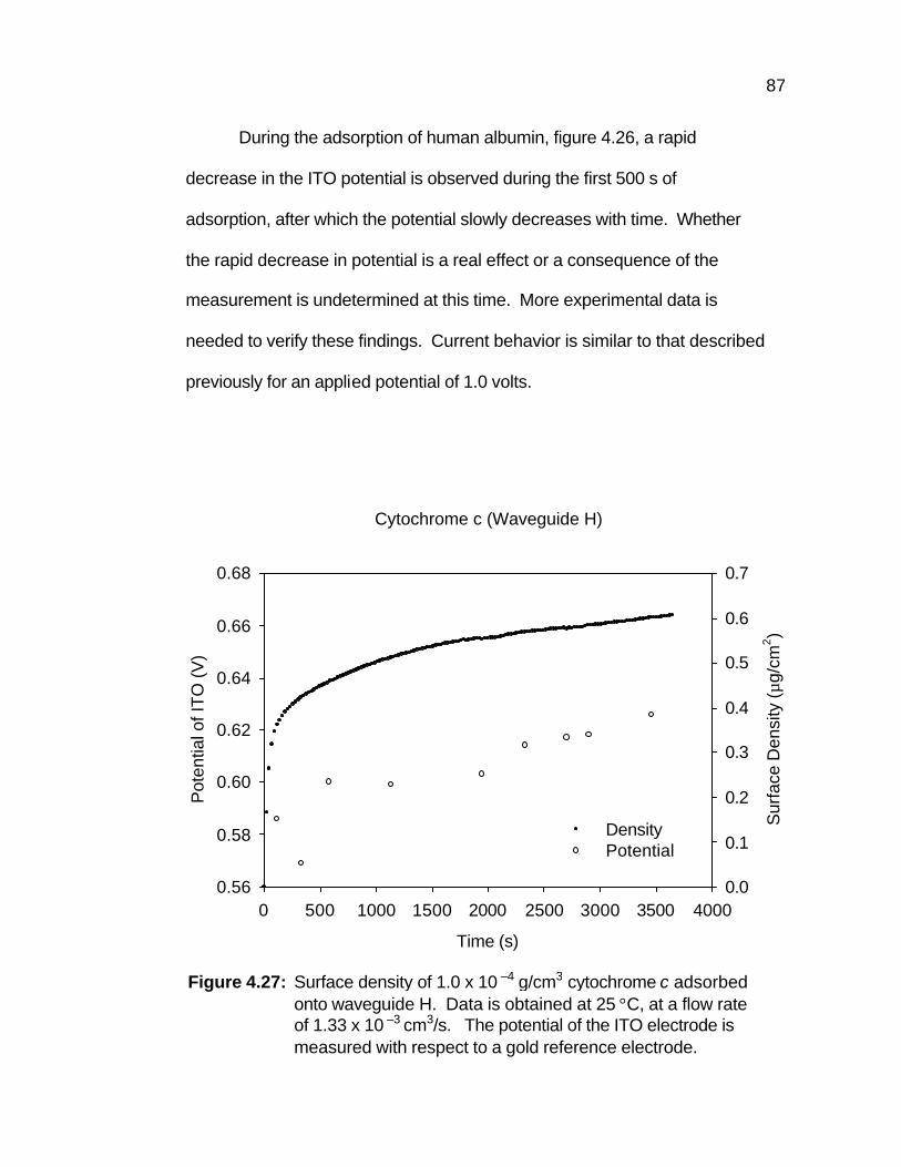
87

During the adsorption of human albumin, figure 4.26, a rapid

decrease in the ITO potential is observed during the first 500 s of

adsorption, after which the potential slowly decreases with time. Whether

the rapid decrease in potential is a real effect or a consequence of the

measurement is undetermined at this time. More experimental data is

needed to verify these findings. Current behavior is similar to that described

previously for an applied potential of 1.0 volts.

Figure 4.27: Surface density of 1.0 x 10 –4 g/cm3 cytochrome c adsorbed onto waveguide H. Data is obtained at 25 °C, at a flow rate of 1.33 x 10 –3 cm3/s. The potential of the ITO electrode is measured with respect to a gold reference electrode.

Cytochrome c (Waveguide H)

Time (s)

0 500 1000 1500 2000 2500 3000 3500 4000

Sur

face

Den

sity

(µg/

cm2 )

0.0

0.1

0.2

0.3

0.4

0.5

0.6

0.7

Pot

entia

l of I

TO

(V

)

0.56

0.58

0.60

0.62

0.64

0.66

0.68

DensityPotential

88

During the adsorption of cytochrome c, figure 4.27, a rapid decrease

in potential is observed during the fist 500 s of adsorption, after which

potential is seen to increase with time. The rapid decrease during the early

stage of adsorption is also observed for the case of albumin. To verify this

affect is real and not a consequence of measurement, additional

experimental are required. Again, current behavior is similar to that

described previously. Current data is presented in Appendix D.

The method presented for measuring electrode potential is in the

preliminary stage of development, however, some generalization about the

experimental results can be made. During the adsorption of albumin and

cytochrome c at an applied potential of 1.0 V current, in general, decreases

with time. Figure 4.26 shows, during the adsorption of albumin, the

electrode potential, for the most part, also decreases with time. A decrease

in current with decreasing electrode potential is expected. However, figure

4.27 shows, a general increase in electrode potential during the adsorption

of cytochrome c. Since current is decreasing with time, this indicates that

some species may be poisoning the electrode.

The next phase of this ongoing research is to further refine the

system. By monitoring and maintaining the electrode potential it may be

possible to determine the reactions occurring at the electrode.

89

4.4 Discussion

In general, two kinetic regimes can describe a protein adsorption

curve, the transport-limited and adsorption-limited regimes. During the initial

stage of adsorption, when no electric field is applied, diffusion is the rate-

limiting step at short times. Following sufficient adsorption to the surface, an

adsorption-limited regime is evident. The adsorption-limited regime can be

divided into two regions, one in which a linear decrease in the adsorption

rate, dΓ/dt, with increasing surface density, Γ, is observed and a second

region in which a non-linear approach to saturation is seen. This discussion

is divided into three sections, which describes the affect of an applied

electric field on protein adsorption in the transport-limited regime and the

two regions of the adsorption-limited regime.

When adsorbing protein in the presence of an electric field, forces

resulting from the field act on the molecules. The magnitude of this force is

dependent on the field strength and the total charge of the molecule.

Experiments are conducted such that the electric field forces acting on a net

negatively charged protein molecules are in the vertical direction toward the

surface, while those acting on a net positively charged molecules are in the

opposite direction. Even though a protein molecule has a net charge

(positive, negative, or neutral), there are both negative and positively

charged groups on the molecule. Because of this, protein molecules will

also align or orient in an electric field due to torque (resulting from forces

acting on the charges through out the molecule).

90

Transient Transport-Limited Regime

The affect of an applied potential on protein adsorption in the

transport-limited regime, where transport to the surface is the rate limiting

mechanism, is analyzed in section 4.3.2. From this analysis, it is found that

the adsorption rates, ∂Γ/∂t, of albumin increases with increasing applied

potential, while the adsorptions rates of cytochrome c and apo-transferrin

are unaffected by the presence of an applied potential in this regime.

When dissolved in deionized water (pH of 5.5 – 6.0), albumin is net

negatively charged. The electric field forces acting on this protein are in the

vertical direction toward the surface. Since an increase adsorption rate is

observed in the transport-limited regime, it is concluded that the magnitude

of the electric field forces acting on this protein are sufficient to enhance the

rate of protein adsorption. Since in this regime the adsorption process is

transport limited, one can infer that electric field induced migration is acting

to increase the effective transport rate for albumin.

Cytochrome c is net positively charged at a pH of 5.5 – 6.0. The

electric field forces acting on this protein should be in the vertical direction

away from the surface, in a direction opposite that of concentration driven

diffusion. The results obtained for cytochrome c show the adsorption rates

are essentially unaffected by an applied electric field. Therefore, it is

concluded that the electric field forces acting on this protein are not sufficient

to impede concentration driven diffusion.

91

At a pH of 5.5 – 6.0, apo-transferrin is close to neutral (or slightly

negatively charged). The results presented in section 4.3.2, show no

noticeable affect on rates of adsorption of this protein. For the case of

neutral molecules it is expected that an applied electric field will have little or

no affect on the rate of adsorption in the transient transport-limited regime,

which is consistent with the experimental findings.

In the presence of an applied electric field, the behavior of albumin

and apo-transferrin in this transport-limited regime are, as one would expect.

However, the behavior of cytochrome c is somewhat surprising. To analyze

this region further, the ratio of the electric field forces to the diffusive forces

(in the absence of an applied electric field), for each of the three proteins at

each of the applied potentials, needs to be determined. To calculate the

electric field induced force acting on a protein molecule, on needs determine

to the strength of the applied field and the apparent charge of the protein

molecule in solution. While the electric field strength can easily be

estimated from current measurements and knowledge of the solution

conductivity, the effective charge of the protein needs to be evaluated

experimentally with electrophoretic measurements. To estimate the

magnitude of the diffusive forces acting on the protein in this initial regime,

one must know the diffusivity of the proteins as well as the concentration

gradients that exist within the flow cell. Theoretical models for the diffusion

of proteins in the initial phases of the adsorption are present by Van Tassel

et. al. [17]. A comparison of these forces may yield some explanation as to

92

why cytochrome c is not affected by the presence of an electric field in this

initial transport limited regime.

Linear Region of the Adsorption-Limited Regime

When surface availability is the rate-limiting mechanism, it is

observed experimentally and predicted theoretically, by Langmuir and other

models, that a linear decrease in the adsorption rate, ∂Γ/∂t, with increasing

adsorbed amounts of protein, Γ, occur. The adsorption rates in this region

are consistent with the protein interacting with the surface (i.e. through the

formation of attractive bonds between the protein and the surface. These

bonds may be physical or chemical in nature). The affect of an applied

potential on protein adsorption in the linear region of the adsorption-limited

regime, is analyzed in section 4.3.3. From this analysis, it is found that the

apparent initial adsorption rate constants, ka, obtained for albumin increase

with increasing applied potential, those obtained for apo-transferrin are only

a slight enhanced, and for cytochrome c, the apparent initial adsorption rate

constants are unaffected. Since surface adsorption is the rate-limiting step

in this region, as described by Langmuir kinetics, one can conclude that the

enhancement in initial rates observed with albumin are not due to electric

field induced migration, as was the case in the transport-limited regime. Of

the three proteins tested, albumin is the only negatively charged protein.

Since the adsorbing surface is positively charged, electrostatic attraction

93

appears to be a likely mechanism. However, surface reactions must also be

considered.

Appling a potential to an electrode affects a number of physical and

chemical properties of the electrode surface, as well as the chemistry of the

solution at the electrode interface. Among these affects are changes in the

hydrophobcity of the electrode surface, localized pH gradients that may

develop near the electrode surface, and the possibility of protein/surface

electron exchange, any of which could possibly have an impact on the

adsorption process. To determine whether the results obtained for albumin

are simply some form of electrostatic attraction or a specific electrochemical

reaction, testing of additional proteins that also have a net negative charge

may provide insight to the nature of the enhancement in initial rate.

Asymptotic Region of the Adsorption-Limited Regime

During the later stage of adsorption, when no potential is applied,

plots of surface density versus time, for each of the three proteins tested,

show an approach to saturation within the time scale of the experiments.

However, when adsorbing protein in the presence of an applied electric field,

the adsorption curves no longer plateau, and a continuous increase in

adsorbed amounts is observed. This is seen for each of the three proteins

at each applied potential (0.5 – 2.0 volts). To look at the affect of an applied

potential on adsorption in the non-linear asymptotic region adsorption-limited

regime, the region of each adsorption curve (presented in section 4.3.1) for t

94

≥ 1800s is analyzed. It has been shown theoretically, by the Simple Particle

Model, that a reversible approach to saturation is exponential and since the

experimental data fit the exponential equation (section 4.3.4, equation 4.1),

it is concluded that the adsorption process in this region is reversible in

nature. From the exponential fit, an asymptotic rate constant, kb, is

obtained. It is observed that the rate constant increases nearly linearly with

increasing applied potential. This behavior is seen with each of the three

proteins tested, despite their difference in chemistry and net charge. Thus

the increase in kb with increasing applied potential is not an affect of electric

field induced migration.

The increase in surface density resulting from an applied potential

may be due one of the following:

1. Tighter packing of the adsorbed protein.

2. A surface reaction with elements common to each of the three

proteins. It is the amino acid side chains that give rise to the unique

properties of proteins. Since it is determined that the later stage of

adsorption is unaffected by protein type (i.e. the differences arising

between each), a reaction could be occurring with elements common

to each protein such as the carboxyl or amino groups.

3. An orientation that favors a higher packing density of adsorbed

protein.

Even though the exact mechanism or factors that account for the observed

effects has not yet been identified, it is evident that an applied potential has

95

a profound affect on adsorption that is highly reproducible over the range of

proteins examined. The ability to deposit multiple and/or thicker protein

layers without higher concentrations, or long adsorption times may have

significant uses in a variety of industrial applications. It seems clear that

both surface density and possibly orientation are influenced by an applied

potential and/or the resulting electric field. The ability to control and alter

these properties would be of great use in creation of biomaterial coatings

and sensing surfaces. Based on the results obtained in this research, this

may be possible with the use of an applied electric field during adsorption.

One concern with this method is that the ITO layer could be changing

with time, as indicated by the measurements of current. At each applied

potential, when deionized water in the flow cell (no protein), there is an

observed decrease in current with time, indicating passivation of the ITO

electrode. At the onset of adsorption, for each of the three proteins tested,

there is an observed current increase at applied potentials of 0.5 and 1.0

volts followed by a continuous decrease. While at applied potentials of 1.5

and 2.0 volts, current may increase, and then gradually decrease

(cytochrome c and apo-transferrin) or it may show a continuous downward

trend (albumin). By measuring and maintaining the ITO electrode potential,

it may be possible to determine what reactions are occurring. Future work in

this area seems promising.

96

5. Conclusion

An important accomplishment here is the modification of an OWLS

biosensor for the continuous measurement of protein adsorption under an

applied electric field. Using this modified system, it is shown that an applied

potential significantly affects the adsorption process. It is found that in the

transient transport-limited regime, an applied potential has a significant

influence on the initial rate of adsorption for albumin, while cytochrome c

and apo-transferrin are unaffected in this region. This implies that, in the

transport-limited regime, the electric field forces acting on albumin are

sufficient to increase the rate of protein transport. In the linear region of the

adsorption-limited regime, it is found that the apparent initial adsorption rate

constants, ka, obtained for albumin increase with increasing applied

potential, those obtained for apo-transferrin are only slightly enhanced, and

for cytochrome c, the apparent initial adsorption rate constants are

unaffected. Given that adsorption in this region is governed by surface

availability, as described Langmuir kinetics, the observed increase in the

initial rate constants seen with albumin must be due to some type of reaction

and not to an increase in transport rate. During the later stage of

adsorption, the density of each of the three proteins tested is considerably

enhanced by the presence of an applied electric field. When a potential of

0.0 V is applied, saturation is reached within the experimental time scale.

However, in the presence larger applied voltages, a continuous increase in

adsorbed amounts of protein is observed. The approach to saturation (for

97

data obtained with and without an applied potential) is found to be

exponential indicating that the adsorption process in this region is not strictly

irreversible in nature. It is observed for each of the three proteins tested that

the asymptotic rate constants, kb, increase similarly with increasing applied

potential. This indicates that the increase in surface density with increasing

applied potential is independent of the protein’s net charge. Kinetic data

such as these are useful for designing electric field methods of controlled

protein-surface placement.

5.1 Future Directions

• Since deionized water is the protein solvent for this work, a pH

gradient near the ITO surface will form. OH- ions will migrate

toward the ITO electrode and may cause the pH near the surface

to be much greater than 5.5-6.0. This would result in albumin,

cytochrome c, and apo-transferrin to be more negatively charged.

Repeating the adsorption experiments presented here with the

proteins being dissolved in a buffer solution (if possible) will

minimize the formation of a pH gradient near the electrode

surface. If the effects described above are due to the presence of

a pH gradient, then testing a buffer solution should have a

significant impact on the experimental findings. However, it is

noted that the use of a buffer solution may reduce electric field

strength, as discussed in section 2.5.

98

• Measure electrode potential during adsorption. Testing at a

constant electrode potential, rather than a constant applied

voltage, may provide insight into protein/surface interactions. In

addition, electrode potentials may prove to be a less system

dependent parameter for the scaling the observed effects than

applied voltage.

• The physical evaluation of surface morphology by techniques

such as AFM may be used to determine the influence of an

applied potential on the final state of the protein-adsorbed layer.

Questions regarding protein packing, orientation, and the

formation of multiple adsorbed layers on the electrode surface

may be answered.

• Examine protein adsorption under cathodic polarization of the

electrode surface rather than anodic. Since prolonged cathodic

polarization changes the optical properties of the ITO electrode,

making it unsuitable for OWLS experiments, other electrodes

needs to be investigated.

99

Appendix A

A.1 Scaled Particle Theory

Scaled Particle Theory is based on an approximate expression for the

work of adding a single solute hard sphere particle of radius R to a system

of hard sphere particles. For the case of protein adsorption, the system of

hard sphere particles is the surface adsorbed proteins. A protein molecule,

from the bulk, will be able to adsorb (be inserted into the system of hard

sphere particles) to the surface if space is made available.

Scaled Particle Theory relates the reversible work required to create

a cavity of radius R that is free from any part of any particle, W(R), to the

probability of finding such a cavity in the equilibrated system Po(R)

where β is the reciprocal of Boltzmann constant times the absolute

temperature. For a 2-D binary mixture of circular particles of radii Rα and Rβ

and densities ρα and ρβ, the value of P0 is known exactly for R=0 and can be

approximated as a power series in R for R>0

[ ]

0RRPR)0(W)0(W

0R)RR()RR(1ln)R(W

2

22

>πβ+′β+β=

≤ρ+π−ρ+π−−=β ββαα

(A.2)

)R(Pln)R(W o−=β (A.1)

100

where P is the pressure of the 2-D binary disk mixture. (Note that a cavity of

negative radius may be thought of as a point that may be approached by a

particle center up to a threshold distance that is less than the particle

radius.)

To obtain W to second order in R, P must be determined. This is

done by noting that the excess chemical potential of species α and β are just

the reversible work required to create cavities of size Rα and Rβ,

respectively: µαex=W(Rα) and µβ

ex =W(Rβ). By differentiating each of these

quantities with respect to ρα, employing the following form of the Gibbs-

Duhem equation,

α

ββ

α

αα

α ∂ρ∂βµ

ρ+∂ρ

∂βµρ=

∂ρ∂β exexexP

solving for the derivative of the excess pressure, and integrating with

respect to ρα, one obtains

[ ]222 RR1

)RR(P

ββαα

βααββα

ρπ−ρπ−

ρρ−π−ρ+ρ=β

The expression obtained for βP is then inserted into equation (A.2) for R>0

to obtain

(A.4)

(A.4)

101

The adsorption probability of the spreading particle model is defined as the

probability of finding a cavity of radius Rα, where Φα = Po(Rα) = exp (-

W(Rα)). The spreading probability is determined as the conditional

probability of finding a cavity of radius Rβ given that a particle of Rα exists at

its center, where Ψαβ = Po(Rβ)/ Po(Rα).

[ ] [ ]

[ ][ ]222

22

2222

RR1

)RR(R

RR1

RRR2RR1ln)R(W

ββαα

βααββα

ββαα

ββααββαα

ρπ−ρπ−

ρρ−π+ρ+ρπ+

ρπ−ρπ−

ρ+ρπ+ρπ−ρπ−−=β (A.5)

102

Appendix B

B.1 Sensor Chip Cleaning

The cleaning procedure for the ITO coated sensor chips is derived

from that of the ASI (type 2400) chips. New ASI (type 2400) sensor chips

are soaked in 0.1 N HCL for 10 minutes then rinsed in deionized water. This

procedure is done only once to remove any residue that may have resulted

from the packing material (i.e. the sensor chips are packaged in a Styrofoam

casing when shipped). After this procedure, the sensor chip is placed in an

ultrasonic bath, containing cleaning solution, at a frequency of 55k Hz for 20

minutes and then rinsed extensively with deionized water. A cleaning

solution at a concentration of 1.0 x 10 - 2

g/cc is prepared by dissolving Terg-

A-Zyme in deionized water.

After a protein adsorption experiment, the ASI type-2400 sensor chip

is cleaned in the ultrasonic bath containing a solution of Terg-A-zyme at the

above mention concentration for 20 minutes, and then rinsed extensively

with deionized water. To determine the effect of the cleaning procedure on

the ASI (type 2400) sensor chip, several experiments are performed. A

sensor chip is placed into the biosensor where the refractive index and

thickness of the film are measured. A 1.0X10 – 4 g/cm3 solution of human

fibrinogen is allowed to flow over the surface of the sensor chip for 30

minutes at a flow rate of 1.33 x 10 – 3 cm3/s and at a temperature of 25 °C.

The chip is then removed from the biosensor and cleaned. After cleaning is

complete, the sensor chip is soaked in the protein solvent (a buffer solution

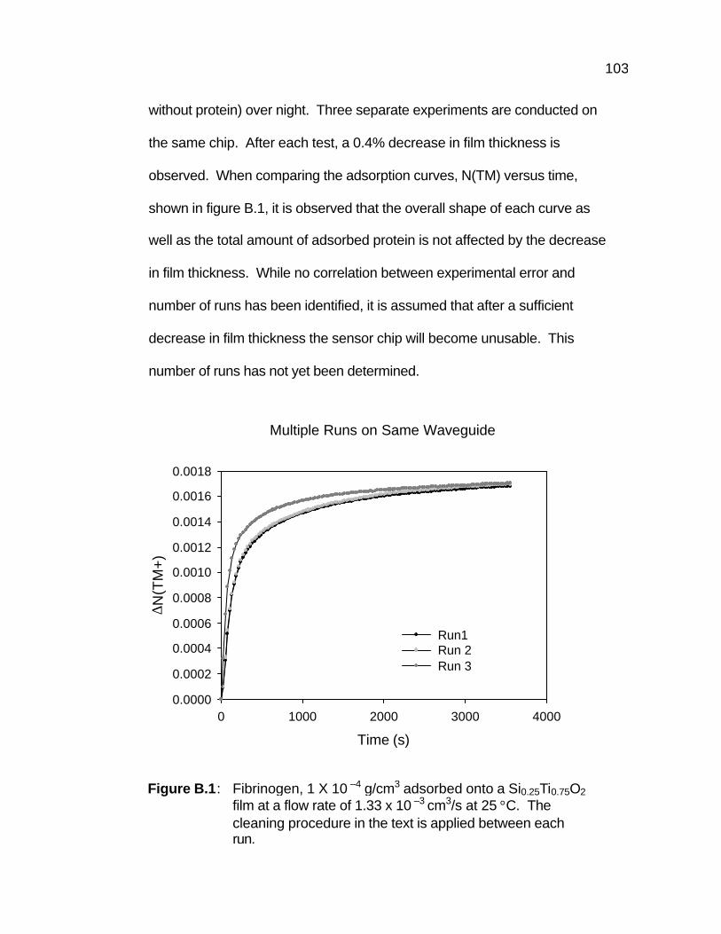
103

without protein) over night. Three separate experiments are conducted on

the same chip. After each test, a 0.4% decrease in film thickness is

observed. When comparing the adsorption curves, N(TM) versus time,

shown in figure B.1, it is observed that the overall shape of each curve as

well as the total amount of adsorbed protein is not affected by the decrease

in film thickness. While no correlation between experimental error and

number of runs has been identified, it is assumed that after a sufficient

decrease in film thickness the sensor chip will become unusable. This

number of runs has not yet been determined.

Multiple Runs on Same Waveguide

Time (s)

0 1000 2000 3000 4000

∆ N(T

M+)

0.0000

0.0002

0.0004

0.0006

0.0008

0.0010

0.0012

0.0014

0.0016

0.0018

Run1Run 2Run 3

Figure B.1: Fibrinogen, 1 X 10 –4 g/cm3 adsorbed onto a Si0.25Ti0.75O2 film at a flow rate of 1.33 x 10 –3 cm3/s at 25 °C. The cleaning procedure in the text is applied between each run.

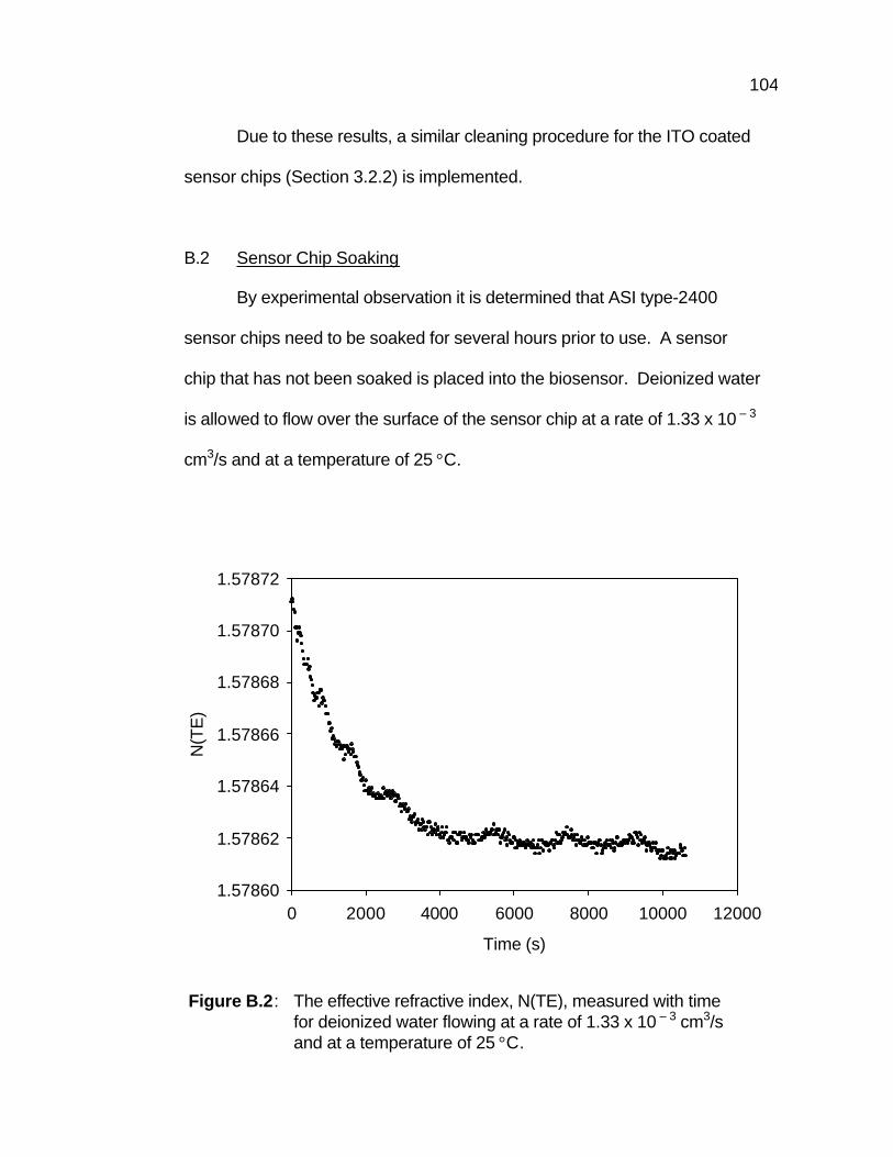
104

Due to these results, a similar cleaning procedure for the ITO coated

sensor chips (Section 3.2.2) is implemented.

B.2 Sensor Chip Soaking

By experimental observation it is determined that ASI type-2400

sensor chips need to be soaked for several hours prior to use. A sensor

chip that has not been soaked is placed into the biosensor. Deionized water

is allowed to flow over the surface of the sensor chip at a rate of 1.33 x 10 – 3

cm3/s and at a temperature of 25 °C.

Time (s)

0 2000 4000 6000 8000 10000 12000

N(T

E)

1.57860

1.57862

1.57864

1.57866

1.57868

1.57870

1.57872

Figure B.2: The effective refractive index, N(TE), measured with time

for deionized water flowing at a rate of 1.33 x 10 – 3 cm3/s and at a temperature of 25 °C.

105

Experiments are performed by measuring the effective refractive indices

N(TM) or N(TE) with time. As shown in figure B.2, it takes several hours for

the effective refractive indices to reach steady state values. Jeremy

Ramsden, of the University of Basle, has also observed this phenomenon.

He attributes this effect to the waveguiding film being porous [22, 30].

Because of these findings, the ITO coated sensor chips are soaked in

deionized water (the protein solvent for this work) for several hours prior to

use.

106

Appendix C

C.1 Fluid Flow

The flow cell of the biosensor allows liquid to be brought in contact

with the film surface of a sensor chip. The flow cell is sealed to the surface

of the sensor chip to create a flow cavity, as described in Section 3.2.4.

Transport limitations are observed inside the cavity when one fluid is

switched with another, as illustrated by the following experiment. At the

beginning of the experiment, the flow channel is filled with deionized water

of refractive index 1.331012 ± 1x10-5 at 25 C°. Glucose dissolved in

deionized water at a concentration 5.0 x 10 – 3 g/cm3 and refractive index

1.33173 ± 1x10-5 at 25 C° (solution indexes measured at 632.8 nm with an

Abbey refractometer, modified by Leica Microsystems, IL, USA) is then

allowed to enter the channel at a rate of 1.33 x 10 – 3 cm3/s. The refractive

index of the solution, at the surface of the sensor chip, is measured with

time.

As seen in Figure C.1, it takes approximately 200 s for the glucose

solution, at the surface of the chip, to reach a maximum refractive index

value. At times t<200 s, the concentration of glucose at the surface of the

chip is transient. At times t > = 200 s, the concentration is that of the bulk.

This observation is attributed to transient diffusion and/or to incomplete

mixing.

Experimental data is compared to refractive index values calculated

for an ideally mixed system where ( )( )Vtexp1CC o ν−−= .

107

C is the concentration of glucose as a function of time, Co is the bulk

concentration,ν is the volumetric flow rate, and V is the volume occupied by

the glucose solution inside of the flow channel. There is a linear relationship

between concentration (0 to 20 x 10 – 2 g/cm3) and the corresponding

measured refractive index values (determined with an Abbey refractometer).

From a plot of refractive index, RI, versus glucose concentration (g/cm3) it is

found that ( ) 1000/1.9357RI1.7030C −= .

Time (s)

0 200 400 600 800 1000

Ref

ract

ive

Inde

x

1.3310

1.3312

1.3314

1.3316

1.3318

ExperimentalIdeal Mixing

Figure C.1: Experimental data of the refractive index of a 5.0 x 10 - 3 g/cm3 glucose solution flowing through the channel at a rate of 1.33 x 10 - 3 cm3/s at 25 °C versus an ideally mixed system.

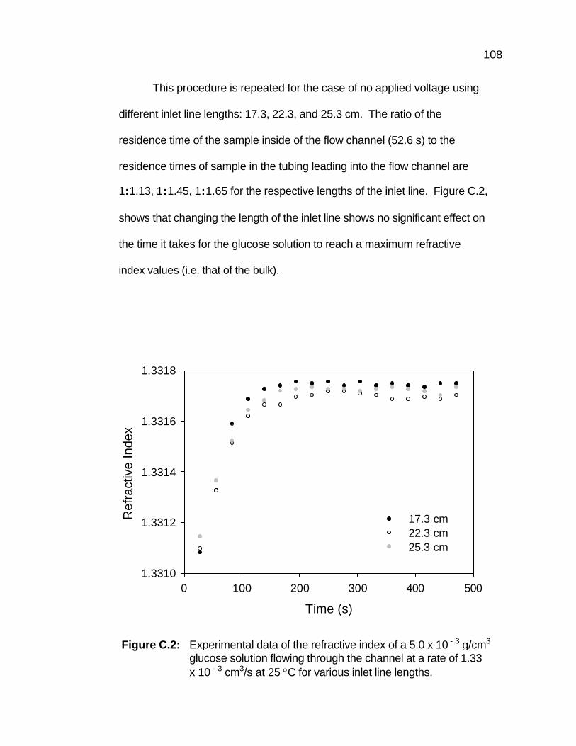
108

This procedure is repeated for the case of no applied voltage using

different inlet line lengths: 17.3, 22.3, and 25.3 cm. The ratio of the

residence time of the sample inside of the flow channel (52.6 s) to the

residence times of sample in the tubing leading into the flow channel are

1:1.13, 1:1.45, 1:1.65 for the respective lengths of the inlet line. Figure C.2,

shows that changing the length of the inlet line shows no significant effect on

the time it takes for the glucose solution to reach a maximum refractive

index values (i.e. that of the bulk).

Time (s)

0 100 200 300 400 500

Ref

ract

ive

Inde

x

1.3310

1.3312

1.3314

1.3316

1.3318

17.3 cm22.3 cm25.3 cm

Figure C.2: Experimental data of the refractive index of a 5.0 x 10 - 3 g/cm3

glucose solution flowing through the channel at a rate of 1.33 x 10 - 3 cm3/s at 25 °C for various inlet line lengths.

109

Appendix D

D.1 Adsorption Data

D.1.1 Human Albumin (Waveguide A)

Figures D.1 through D.5 show the effective refractive indices, N(TE)

and N(TM), as a function of time for the adsorption of 1.0 x 10-4 g/cm3

human albumin onto an ITO coated sensor chip. Data is obtained every

23.5 s at 25°C and at a flow rate of 1.33 x 10-3 cm3/s.

Figure D.1: Effective refractive indices of 1.0 x 10 – 4 g/cm3 human albumin adsorbing onto waveguide A when no voltage is applied to the electrodes. At t= 300 s, the protein solution enters the flow cell. At t=3900 s, a DI water rinse is initiated.

N(TE)N(TM)

Time (s)

0 1000 2000 3000 4000 5000 6000

N(T

E)

1.5710

1.5712

1.5714

1.5716

1.5718

1.5720

N(T

M)

1.5446

1.5448

1.5450

1.5452

1.5454

1.5456

N (TE) N (TM)

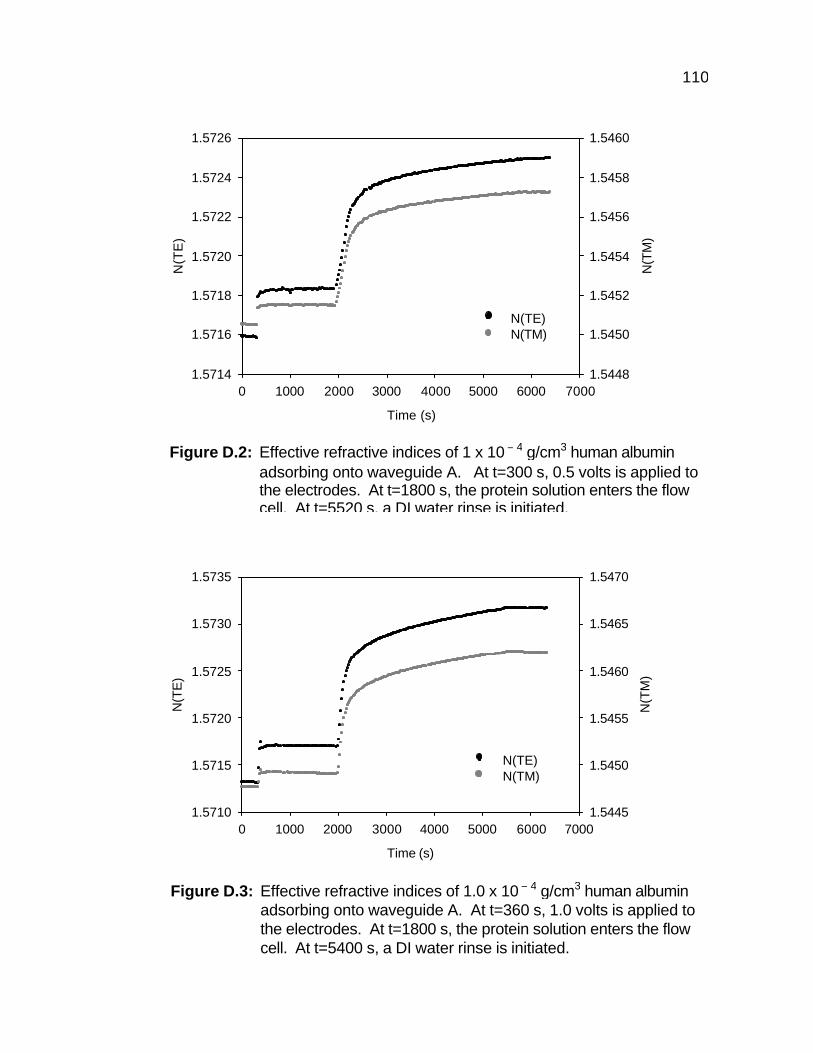
110

Time (s)

0 1000 2000 3000 4000 5000 6000 7000

N(T

E)

1.5714

1.5716

1.5718

1.5720

1.5722

1.5724

1.5726

N(T

M)

1.5448

1.5450

1.5452

1.5454

1.5456

1.5458

1.5460

N(TE)N(TM)

Time (s)

0 1000 2000 3000 4000 5000 6000 7000

N(T

E)

1.5710

1.5715

1.5720

1.5725

1.5730

1.5735

N(T

M)

1.5445

1.5450

1.5455

1.5460

1.5465

1.5470

N(TE) N(TM)

Figure D.2: Effective refractive indices of 1 x 10 – 4 g/cm3 human albumin adsorbing onto waveguide A. At t=300 s, 0.5 volts is applied to the electrodes. At t=1800 s, the protein solution enters the flow cell. At t=5520 s, a DI water rinse is initiated.

Figure D.3: Effective refractive indices of 1.0 x 10 – 4 g/cm3 human albumin adsorbing onto waveguide A. At t=360 s, 1.0 volts is applied to the electrodes. At t=1800 s, the protein solution enters the flow cell. At t=5400 s, a DI water rinse is initiated.

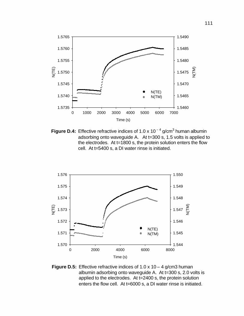
111

Time (s)

0 1000 2000 3000 4000 5000 6000 7000

N(T

E)

1.5735

1.5740

1.5745

1.5750

1.5755

1.5760

1.5765

N(T

M)

1.5460

1.5465

1.5470

1.5475

1.5480

1.5485

1.5490

N(TE) N(TM)

Time (s)

0 2000 4000 6000 8000

N(T

E)

1.570

1.571

1.572

1.573

1.574

1.575

1.576

N(T

M)

1.544

1.545

1.546

1.547

1.548

1.549

1.550

N(TE) N(TM)



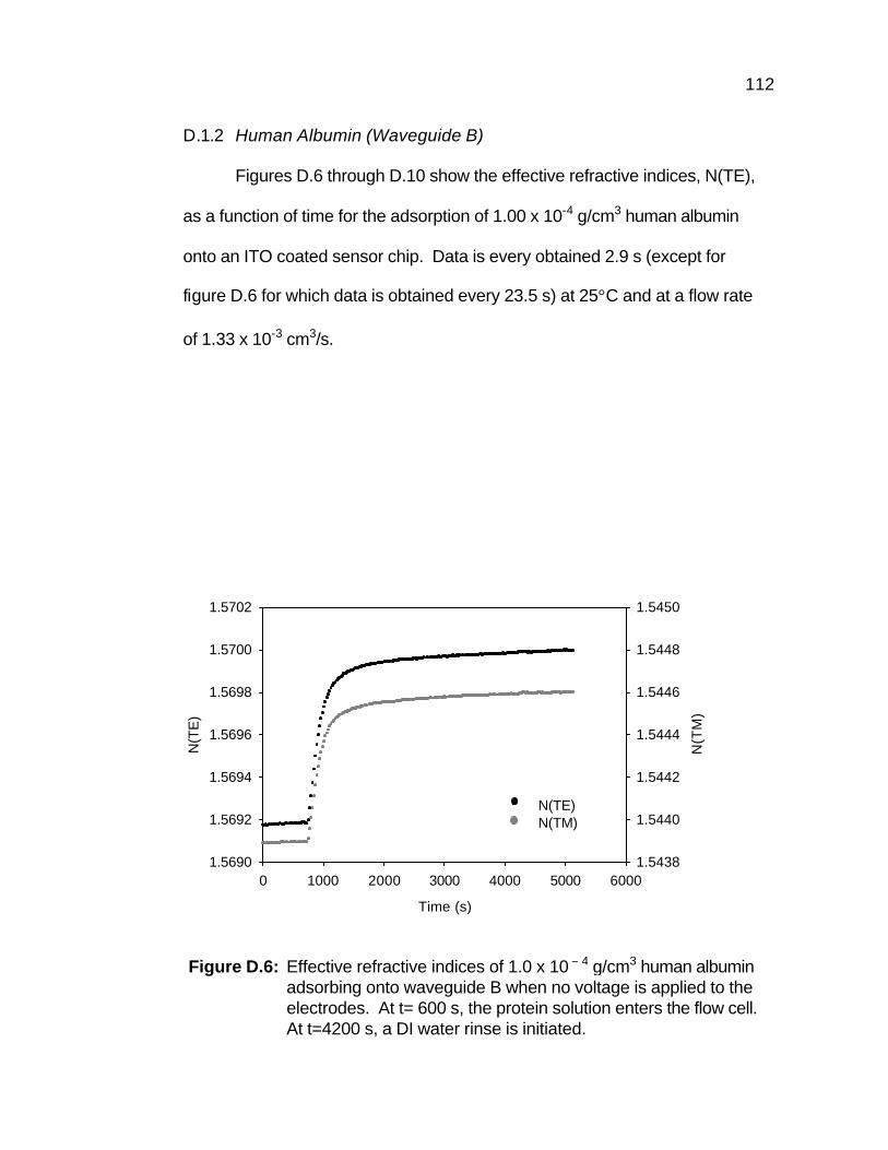
112

D.1.2 Human Albumin (Waveguide B)

Figures D.6 through D.10 show the effective refractive indices, N(TE),

as a function of time for the adsorption of 1.00 x 10-4 g/cm3 human albumin

onto an ITO coated sensor chip. Data is every obtained 2.9 s (except for

figure D.6 for which data is obtained every 23.5 s) at 25°C and at a flow rate

of 1.33 x 10-3 cm3/s.

Time (s)

0 1000 2000 3000 4000 5000 6000

N(T

E)

1.5690

1.5692

1.5694

1.5696

1.5698

1.5700

1.5702

N(T

M)

1.5438

1.5440

1.5442

1.5444

1.5446

1.5448

1.5450

N(TE)N(TM)

Figure D.6: Effective refractive indices of 1.0 x 10 – 4 g/cm3 human albumin adsorbing onto waveguide B when no voltage is applied to the electrodes. At t= 600 s, the protein solution enters the flow cell. At t=4200 s, a DI water rinse is initiated.

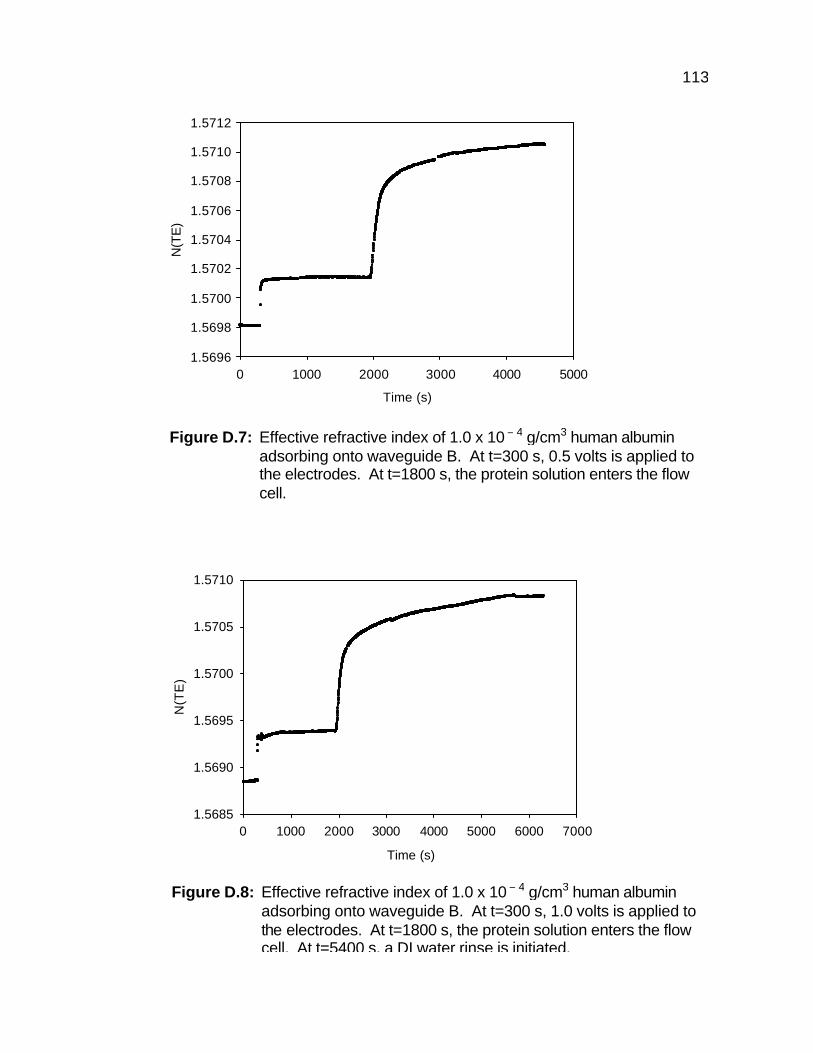
113

Time (s)

0 1000 2000 3000 4000 5000

N(T

E)

1.5696

1.5698

1.5700

1.5702

1.5704

1.5706

1.5708

1.5710

1.5712

Time (s)

0 1000 2000 3000 4000 5000 6000 7000

N(T

E)

1.5685

1.5690

1.5695

1.5700

1.5705

1.5710

Figure D.8: Effective refractive index of 1.0 x 10 – 4 g/cm3 human albumin adsorbing onto waveguide B. At t=300 s, 1.0 volts is applied to the electrodes. At t=1800 s, the protein solution enters the flow cell. At t=5400 s, a DI water rinse is initiated.

Figure D.7: Effective refractive index of 1.0 x 10 – 4 g/cm3 human albumin adsorbing onto waveguide B. At t=300 s, 0.5 volts is applied to the electrodes. At t=1800 s, the protein solution enters the flow cell.

114

Time (s)

0 2000 4000 6000 8000

N(T

E)

1.5695

1.5700

1.5705

1.5710

1.5715

1.5720

1.5725

Time (s)

0 2000 4000 6000 8000

N(T

E)

1.571

1.572

1.573

1.574

1.575

1.576



115

D.1.3 Cytochrome c (Waveguide C)

Figures D.11 through D.15 show the effective refractive indices,

N(TE) and N(TM), as a function of time for the adsorption of 1.0 x 10-4 g/cm3

cytochromce c onto an ITO coated sensor chip. Data is obtained every 23.5

s at 25°C and at a flow rate of 1.33 x 10-3 cm3/s.

Time (s)

0 1000 2000 3000 4000 5000 6000

N(T

E)

1.5690

1.5692

1.5694

1.5696

1.5698

1.5700

1.5702

1.5704

N(T

M)

1.5434

1.5436

1.5438

1.5440

1.5442

1.5444

1.5446

1.5448

N(TE)N(TM)

Figure D.11: Effective refractive indices of 1.0 x 10 – 4 g/cm3 cytochrome c adsorbing onto waveguide C when no voltage is applied to the electrodes. At t= 600 s, the protein solution enters the flow cell. At t=4200 s, a DI water rinse is initiated.

116

Time (s)

0 1000 2000 3000 4000 5000 6000 7000

N(T

E)

1.5702

1.5704

1.5706

1.5708

1.5710

1.5712

N(T

M)

1.5444

1.5446

1.5448

1.5450

1.5452

1.5454

N(TE)N(TM)

Time (s)

0 1000 2000 3000 4000 5000 6000 7000

N(T

E)

1.5692

1.5696

1.5700

1.5704

1.5708

1.5712

N(T

M)

1.5436

1.5440

1.5444

1.5448

1.5452

1.5456

N(TE) N(TM)

Figure D.12: Effective refractive indices of 1.0 x 10 – 4 g/cm3 cytochrome c adsorbing onto waveguide C. At t=300 s, 0.5 volts is applied to the electrodes. At t=1800 s, the protein solution enters the flow cell. At t=5400 s, a DI water rinse is initiated.


117

Time (s)

0 1000 2000 3000 4000 5000 6000 7000

N(T

E)

1.5700

1.5705

1.5710

1.5715

1.5720

1.5725

1.5730

N(T

M)

1.5445

1.5450

1.5455

1.5460

1.5465

1.5470

1.5475

N(TE) N(TM)

Time (s)

0 2000 4000 6000 8000 10000

N(T

E)

1.569

1.570

1.571

1.572

1.573

N(T

M)

1.543

1.544

1.545

1.546

1.547

N(TE) N(TM)



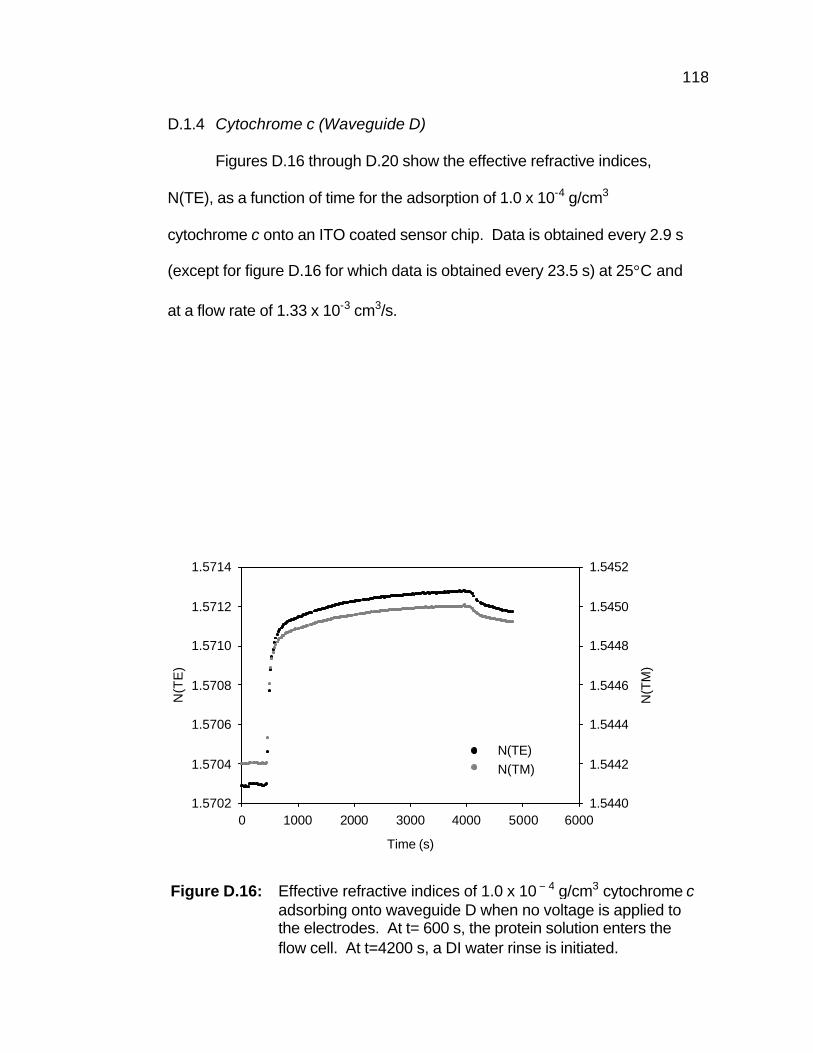
118

D.1.4 Cytochrome c (Waveguide D)


N(TE), as a function of time for the adsorption of 1.0 x 10-4 g/cm3

cytochrome c onto an ITO coated sensor chip. Data is obtained every 2.9 s

(except for figure D.16 for which data is obtained every 23.5 s) at 25°C and

at a flow rate of 1.33 x 10-3 cm3/s.

Time (s)

0 1000 2000 3000 4000 5000 6000

N(T

E)

1.5702

1.5704

1.5706

1.5708

1.5710

1.5712

1.5714

N(T

M)

1.5440

1.5442

1.5444

1.5446

1.5448

1.5450

1.5452

N(TE)N(TM)

Figure D.16: Effective refractive indices of 1.0 x 10 – 4 g/cm3 cytochrome c adsorbing onto waveguide D when no voltage is applied to the electrodes. At t= 600 s, the protein solution enters the flow cell. At t=4200 s, a DI water rinse is initiated.

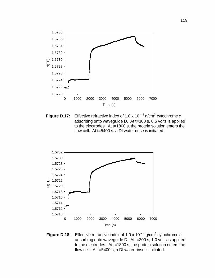
119

Time (s)

0 1000 2000 3000 4000 5000 6000 7000

N(T

E)

1.5720

1.5722

1.5724

1.5726

1.5728

1.5730

1.5732

1.5734

1.5736

1.5738

Time (s)

0 1000 2000 3000 4000 5000 6000 7000

N(T

E)

1.5710

1.5712

1.5714

1.5716

1.5718

1.5720

1.5722

1.5724

1.5726

1.5728

1.5730

1.5732

Figure D.17: Effective refractive index of 1.0 x 10 – 4 g/cm3 cytochrome c adsorbing onto waveguide D. At t=300 s, 0.5 volts is applied to the electrodes. At t=1800 s, the protein solution enters the flow cell. At t=5400 s, a DI water rinse is initiated.


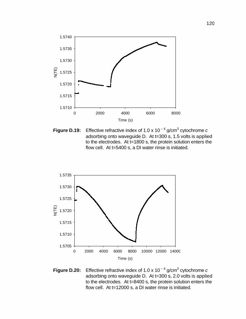
120

Time (s)

0 2000 4000 6000 8000

N(T

E)

1.5710

1.5715

1.5720

1.5725

1.5730

1.5735

1.5740

Time (s)

0 2000 4000 6000 8000 10000 12000 14000

N(T

E)

1.5705

1.5710

1.5715

1.5720

1.5725

1.5730

1.5735



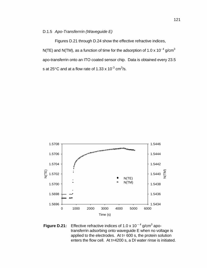
121

D.1.5 Apo-Transferrrin (Waveguide E)


N(TE) and N(TM), as a function of time for the adsorption of 1.0 x 10- 4 g/cm3

apo-transferrin onto an ITO coated sensor chip. Data is obtained every 23.5

s at 25°C and at a flow rate of 1.33 x 10-3 cm3/s.

Time (s)

0 1000 2000 3000 4000 5000 6000

N(T

E)

1.5696

1.5698

1.5700

1.5702

1.5704

1.5706

1.5708

N(T

M)

1.5434

1.5436

1.5438

1.5440

1.5442

1.5444

1.5446

N(TE)N(TM)

Figure D.21: Effective refractive indices of 1.0 x 10 – 4 g/cm3 apo-transferrin adsorbing onto waveguide E when no voltage is applied to the electrodes. At t= 600 s, the protein solution enters the flow cell. At t=4200 s, a DI water rinse is initiated.

122

Time (s)

0 2000 4000 6000 8000

N(T

E)

1.5700

1.5704

1.5708

1.5712

1.5716

1.5720

1.5724

N(T

M)

1.5436

1.5440

1.5444

1.5448

1.5452

1.5456

1.5460

N(TE)N(TM)

Time (s)

0 1000 2000 3000 4000 5000 6000 7000

N(T

E)

1.5755

1.5760

1.5765

1.5770

1.5775

1.5780

1.5785

N(T

M)

1.5465

1.5470

1.5475

1.5480

1.5485

1.5490

1.5495

N(TE) N(TM)

Figure D.22: Effective refractive indices of 1.0 x 10 – 4 g/cm3 apo-transferrin adsorbing onto waveguide E. At t=300 s, 0.5 volts is applied to the electrodes. At t=2400 s, the protein solution enters the flow cell. At t=6000 s, a DI water rinse is initiated.


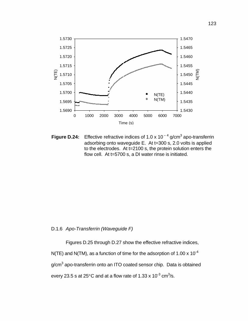
123

Time (s)

0 1000 2000 3000 4000 5000 6000 7000

N(T

E)

1.5690

1.5695

1.5700

1.5705

1.5710

1.5715

1.5720

1.5725

1.5730

N(T

M)

1.5430

1.5435

1.5440

1.5445

1.5450

1.5455

1.5460

1.5465

1.5470

N(TE) N(TM)

D.1.6 Apo-Transferrin (Waveguide F)


N(TE) and N(TM), as a function of time for the adsorption of 1.00 x 10-4

g/cm3 apo-transferrin onto an ITO coated sensor chip. Data is obtained

every 23.5 s at 25°C and at a flow rate of 1.33 x 10-3 cm3/s.


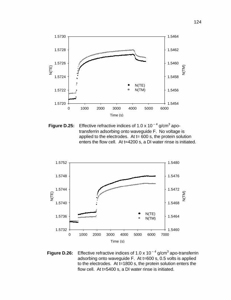
124

Time (s)

0 1000 2000 3000 4000 5000 6000

N(T

E)

1.5720

1.5722

1.5724

1.5726

1.5728

1.5730

N(T

M)

1.5454

1.5456

1.5458

1.5460

1.5462

1.5464

N(TE)N(TM)

Time (s)

0 1000 2000 3000 4000 5000 6000 7000

N(T

E)

1.5732

1.5736

1.5740

1.5744

1.5748

1.5752

N(T

M)

1.5460

1.5464

1.5468

1.5472

1.5476

1.5480

N(TE)N(TM)

Figure D.26: Effective refractive indices of 1.0 x 10 – 4 g/cm3 apo-transferrin adsorbing onto waveguide F. At t=600 s, 0.5 volts is applied to the electrodes. At t=1800 s, the protein solution enters the flow cell. At t=5400 s, a DI water rinse is initiated.

Figure D.25: Effective refractive indices of 1.0 x 10 – 4 g/cm3 apo-transferrin adsorbing onto waveguide F. No voltage is applied to the electrodes. At t= 600 s, the protein solution enters the flow cell. At t=4200 s, a DI water rinse is initiated.

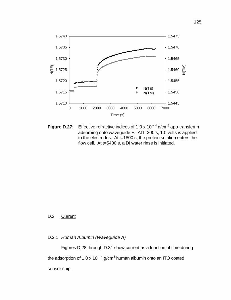
125

Time (s)

0 1000 2000 3000 4000 5000 6000 7000

N(T

E)

1.5710

1.5715

1.5720

1.5725

1.5730

1.5735

1.5740

N(T

M)

1.5445

1.5450

1.5455

1.5460

1.5465

1.5470

1.5475

N(TE) N(TM)

D.2 Current

D.2.1 Human Albumin (Waveguide A)

Figures D.28 through D.31 show current as a function of time during

the adsorption of 1.0 x 10 – 4 g/cm3 human albumin onto an ITO coated

sensor chip.

Figure D.27: Effective refractive indices of 1.0 x 10 – 4 g/cm3 apo-transferrin adsorbing onto waveguide F. At t=300 s, 1.0 volts is applied to the electrodes. At t=1800 s, the protein solution enters the flow cell. At t=5400 s, a DI water rinse is initiated.

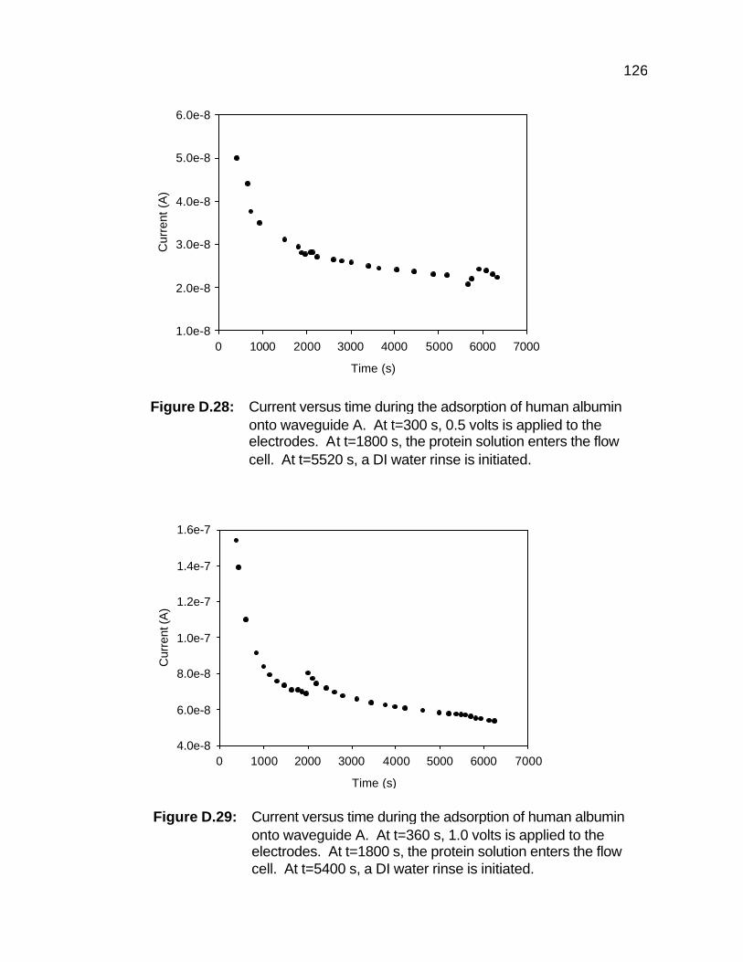
126

Time (s)

0 1000 2000 3000 4000 5000 6000 7000

Cur

rent

(A

)

1.0e-8

2.0e-8

3.0e-8

4.0e-8

5.0e-8

6.0e-8

Time (s)

0 1000 2000 3000 4000 5000 6000 7000

Cur

rent

(A)

4.0e-8

6.0e-8

8.0e-8

1.0e-7

1.2e-7

1.4e-7

1.6e-7

Figure D.28: Current versus time during the adsorption of human albumin onto waveguide A. At t=300 s, 0.5 volts is applied to the electrodes. At t=1800 s, the protein solution enters the flow cell. At t=5520 s, a DI water rinse is initiated.


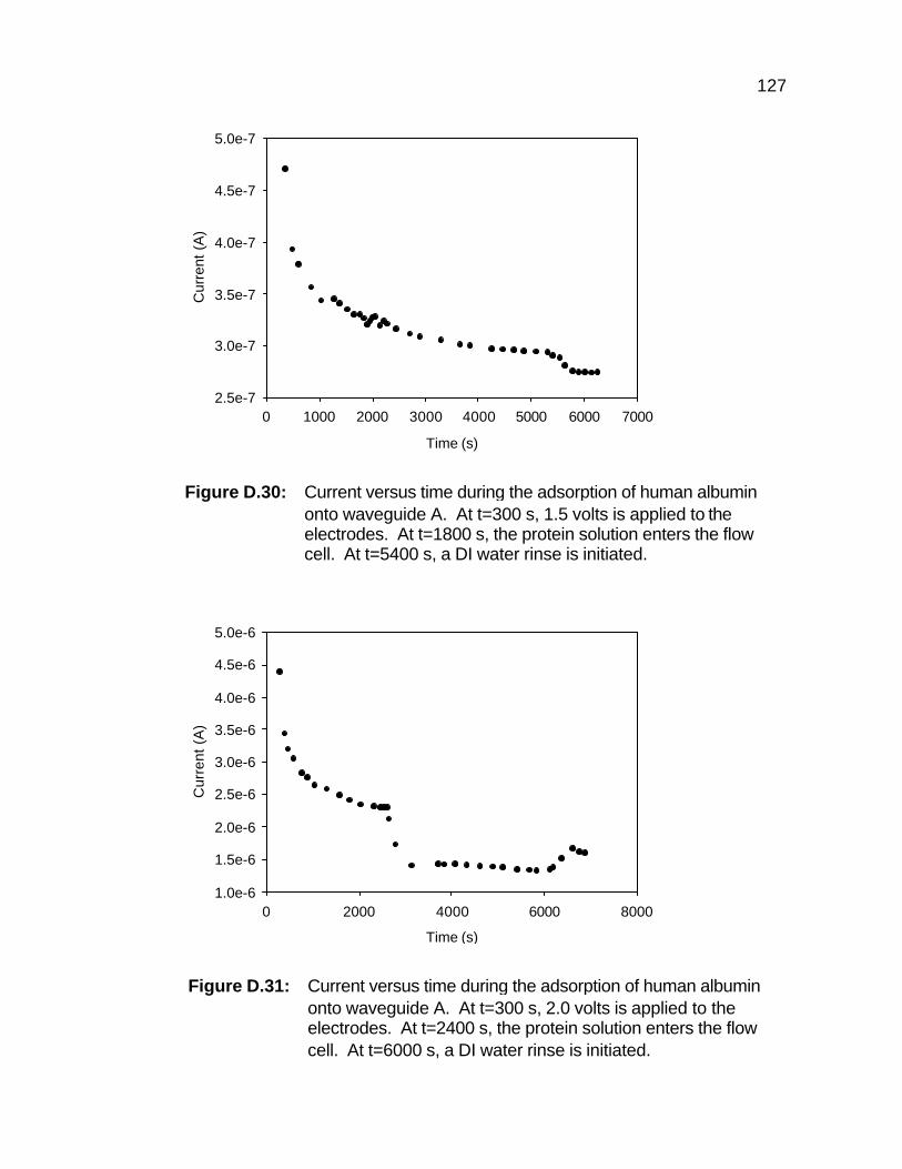
127

Time (s)

0 1000 2000 3000 4000 5000 6000 7000

Cur

rent

(A

)

2.5e-7

3.0e-7

3.5e-7

4.0e-7

4.5e-7

5.0e-7

Time (s)

0 2000 4000 6000 8000

Cur

rent

(A

)

1.0e-6

1.5e-6

2.0e-6

2.5e-6

3.0e-6

3.5e-6

4.0e-6

4.5e-6

5.0e-6



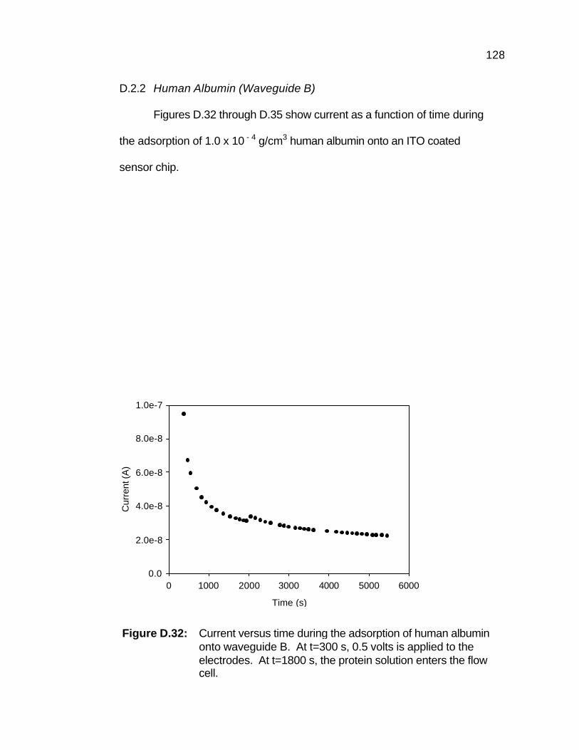
128

D.2.2 Human Albumin (Waveguide B)


the adsorption of 1.0 x 10 - 4 g/cm3 human albumin onto an ITO coated

sensor chip.

Time (s)

0 1000 2000 3000 4000 5000 6000

Cur

rent

(A)

0.0

2.0e-8

4.0e-8

6.0e-8

8.0e-8

1.0e-7

Figure D.32: Current versus time during the adsorption of human albumin onto waveguide B. At t=300 s, 0.5 volts is applied to the electrodes. At t=1800 s, the protein solution enters the flow cell.

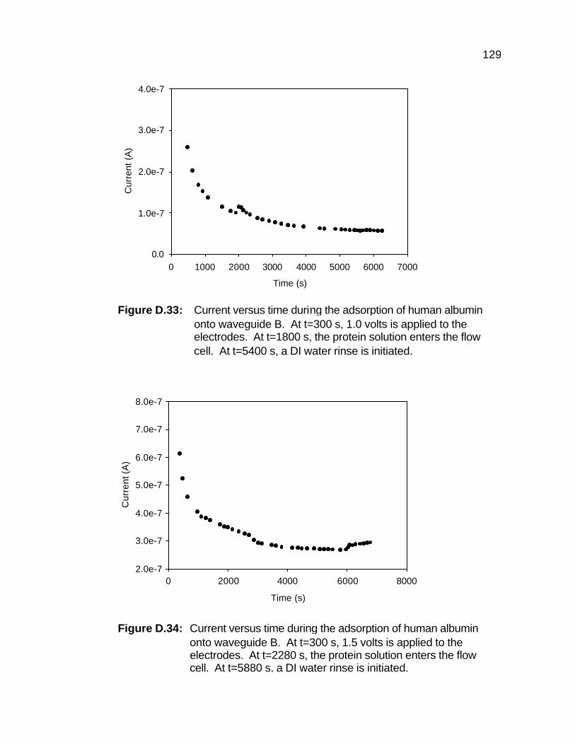
129

Time (s)

0 1000 2000 3000 4000 5000 6000 7000

Cur

rent

(A

)

0.0

1.0e-7

2.0e-7

3.0e-7

4.0e-7

Time (s)

0 2000 4000 6000 8000

Cur

rent

(A)

2.0e-7

3.0e-7

4.0e-7

5.0e-7

6.0e-7

7.0e-7

8.0e-7

Figure D.33: Current versus time during the adsorption of human albumin onto waveguide B. At t=300 s, 1.0 volts is applied to the electrodes. At t=1800 s, the protein solution enters the flow cell. At t=5400 s, a DI water rinse is initiated.


130

Time (s)

0 2000 4000 6000 8000

Cur

rent

(A

)

8.0e-7

1.2e-6

1.6e-6

2.0e-6

2.4e-6

2.8e-6

3.2e-6

D.2.3 Cytochrome c (Waveguide C)


the adsorption of 1.0 x 10 - 4 g/cm3 cytochromce c onto an ITO coated

sensor chip.


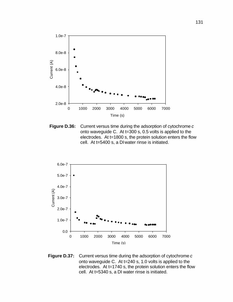
131

Time (s)

0 1000 2000 3000 4000 5000 6000 7000

Cur

rent

(A

)

2.0e-8

4.0e-8

6.0e-8

8.0e-8

1.0e-7

Time (s)

0 1000 2000 3000 4000 5000 6000 7000

Cur

rent

(A)

0.0

1.0e-7

2.0e-7

3.0e-7

4.0e-7

5.0e-7

6.0e-7

Figure D.37: Current versus time during the adsorption of cytochrome c onto waveguide C. At t=240 s, 1.0 volts is applied to the electrodes. At t=1740 s, the protein solution enters the flow cell. At t=5340 s, a DI water rinse is initiated.


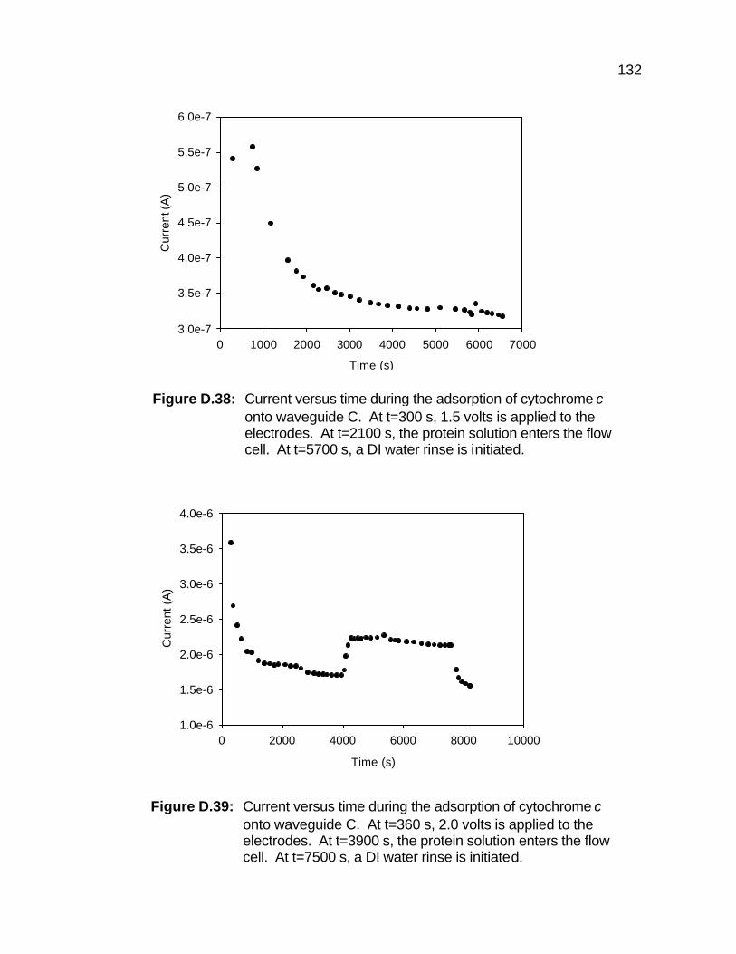
132

Time (s)

0 1000 2000 3000 4000 5000 6000 7000

Cur

rent

(A)

3.0e-7

3.5e-7

4.0e-7

4.5e-7

5.0e-7

5.5e-7

6.0e-7

Time (s)

0 2000 4000 6000 8000 10000

Cur

rent

(A

)

1.0e-6

1.5e-6

2.0e-6

2.5e-6

3.0e-6

3.5e-6

4.0e-6



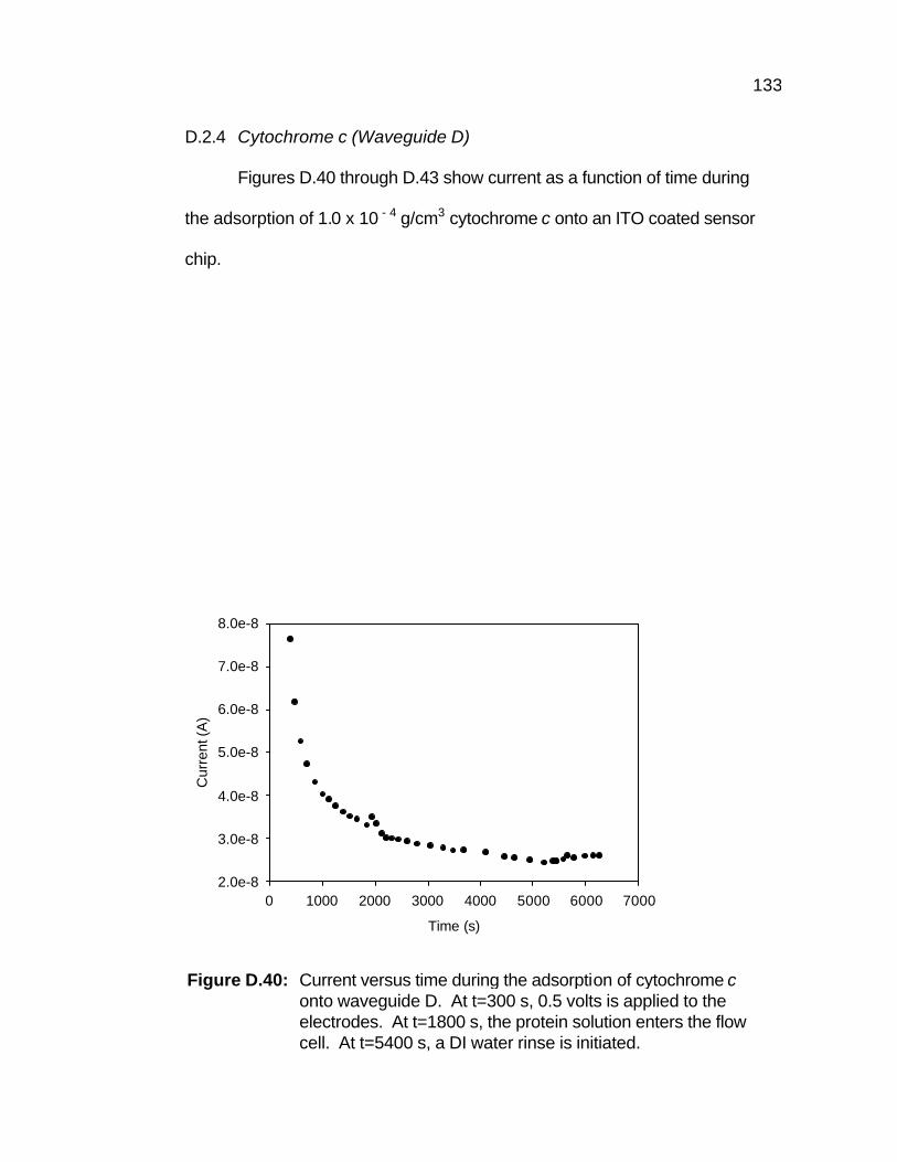
133

D.2.4 Cytochrome c (Waveguide D)


the adsorption of 1.0 x 10 - 4 g/cm3 cytochrome c onto an ITO coated sensor

chip.

Time (s)

0 1000 2000 3000 4000 5000 6000 7000

Cur

rent

(A)

2.0e-8

3.0e-8

4.0e-8

5.0e-8

6.0e-8

7.0e-8

8.0e-8

Figure D.40: Current versus time during the adsorption of cytochrome c

onto waveguide D. At t=300 s, 0.5 volts is applied to the electrodes. At t=1800 s, the protein solution enters the flow cell. At t=5400 s, a DI water rinse is initiated.

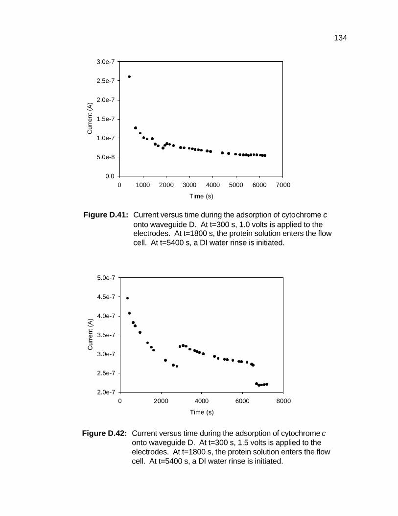
134

Time (s)

0 1000 2000 3000 4000 5000 6000 7000

Cur

rent

(A

)

0.0

5.0e-8

1.0e-7

1.5e-7

2.0e-7

2.5e-7

3.0e-7

Time (s)

0 2000 4000 6000 8000

Cur

rent

(A

)

2.0e-7

2.5e-7

3.0e-7

3.5e-7

4.0e-7

4.5e-7

5.0e-7

Figure D.41: Current versus time during the adsorption of cytochrome c onto waveguide D. At t=300 s, 1.0 volts is applied to the electrodes. At t=1800 s, the protein solution enters the flow cell. At t=5400 s, a DI water rinse is initiated.


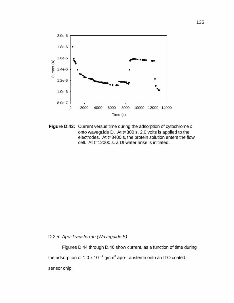
135

Time (s)

0 2000 4000 6000 8000 10000 12000 14000

Cur

rent

(A

)

8.0e-7

1.0e-6

1.2e-6

1.4e-6

1.6e-6

1.8e-6

2.0e-6

D.2.5 Apo-Transferrrin (Waveguide E)

Figures D.44 through D.46 show current, as a function of time during

the adsorption of 1.0 x 10 - 4 g/cm3 apo-transferrin onto an ITO coated

sensor chip.


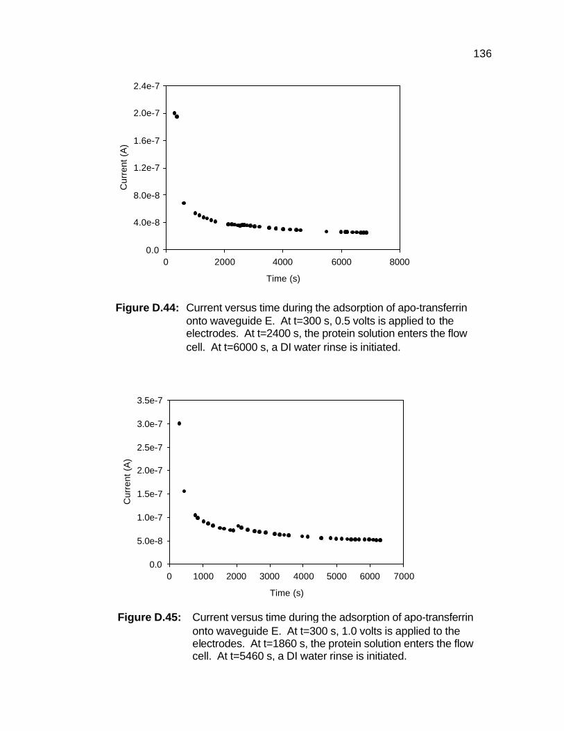
136

Time (s)

0 2000 4000 6000 8000

Cur

rent

(A

)

0.0

4.0e-8

8.0e-8

1.2e-7

1.6e-7

2.0e-7

2.4e-7

Time (s)

0 1000 2000 3000 4000 5000 6000 7000

Cur

rent

(A

)

0.0

5.0e-8

1.0e-7

1.5e-7

2.0e-7

2.5e-7

3.0e-7

3.5e-7

Figure D.44: Current versus time during the adsorption of apo-transferrin onto waveguide E. At t=300 s, 0.5 volts is applied to the electrodes. At t=2400 s, the protein solution enters the flow cell. At t=6000 s, a DI water rinse is initiated.


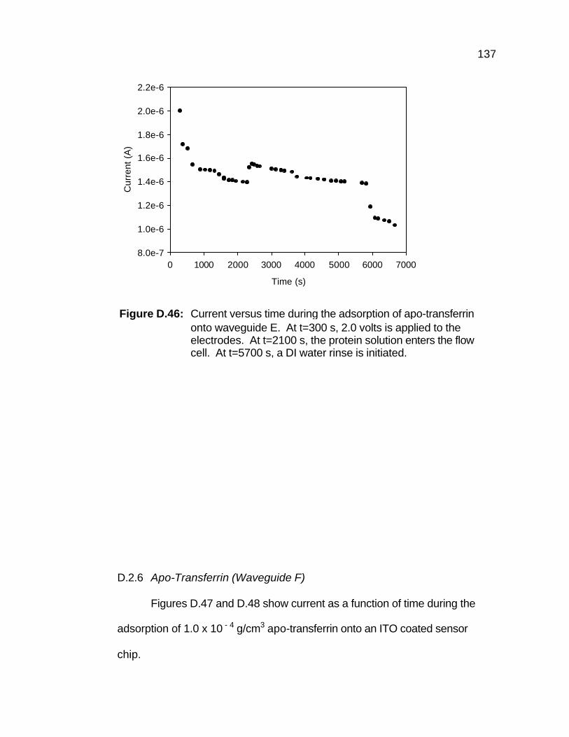
137

Time (s)

0 1000 2000 3000 4000 5000 6000 7000

Cur

rent

(A

)

8.0e-7

1.0e-6

1.2e-6

1.4e-6

1.6e-6

1.8e-6

2.0e-6

2.2e-6

D.2.6 Apo-Transferrin (Waveguide F)

Figures D.47 and D.48 show current as a function of time during the

adsorption of 1.0 x 10 - 4 g/cm3 apo-transferrin onto an ITO coated sensor

chip.


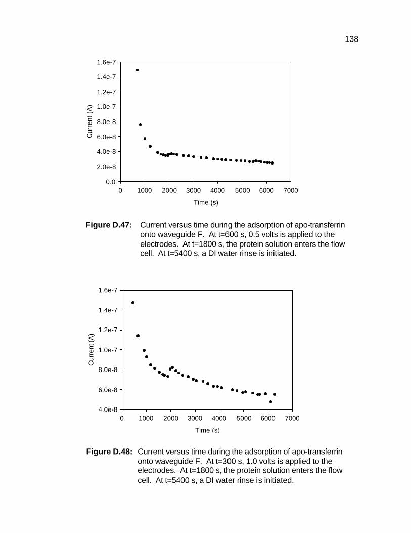
138

Time (s)

0 1000 2000 3000 4000 5000 6000 7000

Cur

rent

(A

)

0.0

2.0e-8

4.0e-8

6.0e-8

8.0e-8

1.0e-7

1.2e-7

1.4e-7

1.6e-7

Time (s)

0 1000 2000 3000 4000 5000 6000 7000

Cur

rent

(A)

4.0e-8

6.0e-8

8.0e-8

1.0e-7

1.2e-7

1.4e-7

1.6e-7

Figure D.48: Current versus time during the adsorption of apo-transferrin onto waveguide F. At t=300 s, 1.0 volts is applied to the electrodes. At t=1800 s, the protein solution enters the flow cell. At t=5400 s, a DI water rinse is initiated.

Figure D.47: Current versus time during the adsorption of apo-transferrin onto waveguide F. At t=600 s, 0.5 volts is applied to the electrodes. At t=1800 s, the protein solution enters the flow cell. At t=5400 s, a DI water rinse is initiated.

139

D.3 Electrode Potential

D.3.1 Albumin (Waveguide G)

Figure D.49 shows the effective refractive indices, N(TE) and N(TM),

as a function of time for the adsorption of 1.0 x 10 - 4 g/cm3 human albumin

onto an ITO coated sensor chip. Data is obtained every 23.5 s at 25°C and

at a flow rate of 1.33 x 10 - 3 cm3/s.

Time (s)

0 1000 2000 3000 4000 5000 6000 7000

N(T

E)

1.5836

1.5838

1.5840

1.5842

1.5844

1.5846

1.5848

1.5850

N(T

M)

1.5554

1.5556

1.5558

1.5560

1.5562

1.5564

1.5566

1.5568

N(TE)N(TM)

Figure D.49: Effective refractive indices for 1.0 x 10 – 4 g/cm3 human albumin adsorbed onto waveguide G. At t=300 s, 1.0 volts is applied to the electrodes. At t=2563 s, the protein solution enters the flow cell.

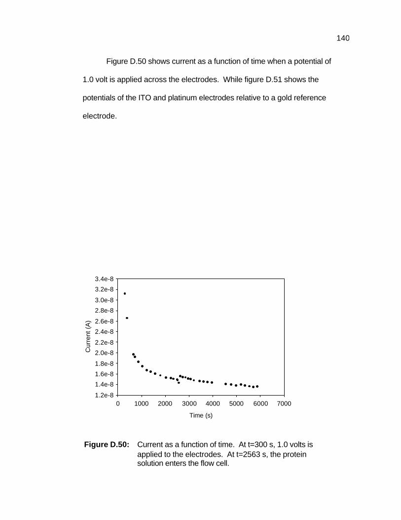
140

Figure D.50 shows current as a function of time when a potential of

1.0 volt is applied across the electrodes. While figure D.51 shows the

potentials of the ITO and platinum electrodes relative to a gold reference

electrode.

Time (s)

0 1000 2000 3000 4000 5000 6000 7000

Cur

rent

(A

)

1.2e-8

1.4e-8

1.6e-8

1.8e-8

2.0e-8

2.2e-8

2.4e-8

2.6e-8

2.8e-8

3.0e-8

3.2e-8

3.4e-8

Figure D.50: Current as a function of time. At t=300 s, 1.0 volts is applied to the electrodes. At t=2563 s, the protein solution enters the flow cell.

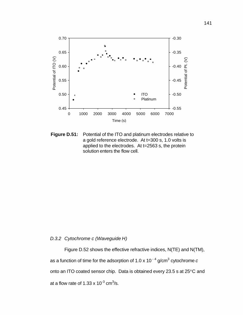
141

Time (s)

0 1000 2000 3000 4000 5000 6000 7000

Pot

entia

l of I

TO

(V

)

0.45

0.50

0.55

0.60

0.65

0.70

Pot

entia

l of P

t. (V

)

-0.55

-0.50

-0.45

-0.40

-0.35

-0.30

ITOPlatinum

D.3.2 Cytochrome c (Waveguide H)

Figure D.52 shows the effective refractive indices, N(TE) and N(TM),

as a function of time for the adsorption of 1.0 x 10 - 4 g/cm3 cytochrome c

onto an ITO coated sensor chip. Data is obtained every 23.5 s at 25°C and

at a flow rate of 1.33 x 10-3 cm3/s.

Figure D.51: Potential of the ITO and platinum electrodes relative to a gold reference electrode. At t=300 s, 1.0 volts is applied to the electrodes. At t=2563 s, the protein solution enters the flow cell.

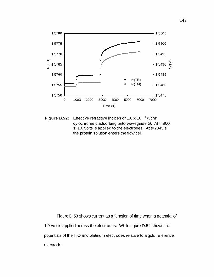
142

Time (s)

0 1000 2000 3000 4000 5000 6000 7000

N(T

E)

1.5750

1.5755

1.5760

1.5765

1.5770

1.5775

1.5780

N(T

M)

1.5475

1.5480

1.5485

1.5490

1.5495

1.5500

1.5505

N(TE)N(TM)

Figure D.53 shows current as a function of time when a potential of

1.0 volt is applied across the electrodes. While figure D.54 shows the

potentials of the ITO and platinum electrodes relative to a gold reference

electrode.

Figure D.52: Effective refractive indices of 1.0 x 10 – 4 g/cm3

cytochrome c adsorbing onto waveguide G. At t=900 s, 1.0 volts is applied to the electrodes. At t=2845 s, the protein solution enters the flow cell.

143

Time (s)

0 1000 2000 3000 4000 5000 6000 7000

Pot

entia

l of I

TO

(V)

0.40

0.45

0.50

0.55

0.60

0.65

0.70

Pot

entia

l of P

t. (V

)

-0.54

-0.52

-0.50

-0.48

-0.46

-0.44

-0.42

-0.40

-0.38

-0.36

ITOPlatinum

Figure D.53: Current as a function of time. At t=900 s, 1.0 volts is applied to the electrodes. At t=2845 s, the protein solution enters the flow cell.

Figure D.54: Potential of the ITO and platinum electrodes relative to a gold reference electrode. At t=900 s, 1.0 volts is applied to the electrodes. At t=2845 s, the protein solution enters the flow cell.

Time (s)

0 1000 2000 3000 4000 5000 6000 7000

Cur

rent

(A

)

1.6e-8

1.8e-8

2.0e-8

2.2e-8

2.4e-8

2.6e-8

2.8e-8

3.0e-8

3.2e-8

3.4e-8

144

References

1. Asanov, A. N., Wilson, W. W., Oldham, P. B., Anal. Chem. 70, 1115-

1163 (1998).

2. Asanov, A.N., DeLucas, L.J., Oldham, P.B., and Wilson, W.W., J.

Colloid Interface Sci. 191, 222 (1997).

3. Fraaije, J.G.E.M., Kleijn, J.M. and VanDerGraaf, M., Biophysical

Journal 57, 965-976 (1990).

4. Fievet, P., Mullet, M., Reggiani, J.C., Pagetti, J., Colloids and

Surfaces A: Physicochem. Eng. Aspects 144, 35-42 (1998).

5. Bernabeu, P. and Caprani, A., Biomaterials 11 (4), 258-264 (1990).

6. Garrett, R. H., Grisham, G. M., Biochemistry, 2nd ed., Saunders

College Publishing, 1999: 107, 159, 172.

7. Atkins, P., Physical Chemistry, 5th ed., New York, W. H. Freeman and

Company, 1994: 987.

8. Schaaf, P., and Talbot, J., Phys. Rev. Lett. 62, 175 (1989).

9. Tarjus, G., Schaaf, P., and Talbot, J., J. Stat. Phys. 63, 167 (1991).

10. Evans, J. W., Rev. Mod. Phys. 65, 1281 (1993).

11. Adamczyk, Z., Siweck, B., Zembala, M., and Belouscheck, P., Adv.

Colloid Surf. 48, 151 (1994).

12. Van Tassel, P. R., Viot, P., Tarjus G., J. Chem. Phys. 106 (2) 761-

769 (1997).

13. Van Tassel, P. R., Talbot, J., Tarjus, G., and Viot, P., Physical

Review E 53 (1), 785-798 (1996).

145

14. Brusatori, M. A., Van Tassel, P. R., Journal of Colloid and Interface

Science 219 (2), 333-338 (1999).

15. Lebowitz, J. L., Helfand, E., Praestgaard, E., Journal of Chemical

Physics 43 (3), 774-779 (1965).

16. Van Tassel, P. R., et. al., Langmuir 17 4392-4395 (2001).

17. Van Tassel, P. R., et. al., Biophysics, publication pending.

18. Guemouri, L., Ojier, J., and Ramsden, J. J., J. of Chemical Physics

109 (8), 3265-3268 (1998).

19. Ramsden, J. J., and Mate, M., J. Chem. Soc., Faraday Trans., 94 (6)

783-788 (1998).

20. Kurrat, R., Prenosil, J. E., Ramsden, J. J., J. of Colloid and Interface

Science 185, 1 – 8 (1997).

21. Lukosz, W. and Tiefenthaler, K., Sensors and Actuators 15, 273-284

(1988).

22. Nellen, PH. M. and Lukosz, W., Sensors and Actuators B1, 592-596

(1990).

23. Tiefenthaler, K. and Lukosz, W., J. Opt. Soc. Am. B 6, 209 (1989).

24. Lukosz, W., Sensors Actuators B 29, 37 (1995).

25. Manual provide with the optical biosensor, BIOS-1, Artificial Sensing

Instrument (ASI AG), Zurich, Switzerland.

26. Jackson, John David, Classical Electrodynamics, 3rd ed., John Wiley

& Sons, Inc., 1999: 302 – 308, 385, 386.

27. Sigma Chemical Company, Saint Louis Missouri, USA.

146

28. Fasman, Gerald, D., ed., Handbook of Biochemistry and Molecular

Biology, 3d ed., 5 Vols, Cleveland: CRC Press, c1975-1977, Vol. 2.

29. Luff, Jonathan J., Wilkinson, James S., Perrone, Guido, Applied

Optics 36 (27), 7066-7072 (1997).

30. Ramsden, J.J., J. Mater. Chem. 4 (8), 1263-1265 (1994).

31. Brusatori, Michelle, A., Van Tassel, Paul, R., Journal of Colloid and

Interface Science, submitted (2001).

32. Wangsness, Ronald K., Electromagnetic Fields, 2nd ed., John Wiley &

Sons, Inc., 1986: 405 - 421.

33. Hecht, Eugene, Optics, 3rd ed., Addison Wesley Longman, Inc., 1998:

109 - 126.

147

Abstract

PROTEIN ADSORPTION KINETICS UNDER AN APPLIED ELECTRIC FIELD: AN OPTICAL WAVEGUIDE LIGHTMODE SPECTROSCOPY STUDY

by


December 2001

Advisor: Dr. Paul Van Tassel Major: Chemical Engineering Degree: Doctor of Philosophy

The controlled placement of protein molecules onto surfaces represents

a crucial step toward many new biotechnological devices and processes. An

applied electric field offers a promising means of controlling the rate of

adsorption to the surface and the structure of the adsorbed layer. A method for

monitoring the time evolution of an adsorbed protein layer in the presence of

an electric field is presented. In this work, Optical Waveguide Lightmode

Spectroscopy (OWLS) is used to measure the mass and layer thickness of

protein adsorbing onto an indium tin oxide (ITO) electrode. Over a range of

applied potentials, a kinetic analysis of human albumin, cytochrome c, and

apo-transferrin is performed to determine the affects of surface and protein

charge and electrochemical properties of the electrode surface on the

adsorption process. It is found that in the transport-limited regime an applied

potential has a significant influence on the initial rate of adsorption of albumin,

148

while cytochrome c and apo-transferrin are unaffected in this region. During

the later stage of adsorption the density of each of the three proteins tested is

considerably enhanced by the presence of an applied electric field. This

enhancement is found to be independent of the net charge of the protein.

149

Autobiographical Statement Name: Michelle A. Brusatori

Date of Birth: June 13, 1965, Detroit, MI.

Education: ♦ Ph.D. Chemical Engineering, Dec. 2001 Minor in Physics Wayne State University, Detroit, MI. ♦ MS Chemical Engineering, May 1998 Wayne State University, Detroit, MI. ♦ BS Chemical Engineering, May 1996 Wayne State University, Detroit, MI. Experience: ♦ Graduate Research Assistant, May 1998 – Dec. 2001 Wayne State University, Detroit, MI.

♦ Graduate Teaching Assistant, Sept. 1996 – May 1998 Wayne State University, Detroit, MI.

♦ Undergraduate Research, May 1995 – Sept. 1996 Wayne State University, Detroit, MI.

♦ Production Manager

July 1984 – Dec. 1989 Alden design Inc., Sterling Heights, MI. Areas of Interest: ♦ Protein Adsorption Kinetics and Surface Reactions

♦ Optics ♦ Electromagnetic Theory

Awards ♦ College of Engineering Excellence in Teaching Award Wayne State University, 1997

protein adsorption kinetics under an applied

Documents