protein-protein-interaction networks · pdf fileulf leser: bioinformatics, summer semester...
TRANSCRIPT

Protein-Protein-Interaction Networks
Ulf Leser, Samira Jaeger

Ulf Leser: Bioinformatics, Summer Semester 2016 2
This Lecture
• Protein-protein interactions– Characteristics– Experimental detection methods– Databases
• Biological networks

Ulf Leser: Bioinformatics, Summer Semester 2016 3
Motivation
• Interaction: Physical binding of two or more proteins– E.g. signal transduction, gene regulation, metabolism, …– Transient or permanent– Directed effect (regulates), undirected (binds), specific
(activates)• Changes in protein structure may hinder bindings and
thus perturb natural cellular processes– Influence on all “downstream” proteins, i.e., proteins
reachable through a path of interactions• Interactome: Set of all PPIs in a cell (type, species, …)• Complex: Permanent binding of two or more proteins

Ulf Leser: Bioinformatics, Summer Semester 2016 4
Context-dependency
• PPI often is context-dependent– Cell type, cell cycle phase and state– Environmental conditions– Developmental stage– Protein modification– Presence of cofactors and other binding partners– …
• Disregarded by many PPI detection methods• Low quality of typical data sets

Ulf Leser: Bioinformatics, Summer Semester 2016 5
Experimental detection methods
• PPIs have been studied extensively using different experimental methods
• Many are small-scale: Two given proteins in a given condition
• High-throughput methods• Yeast two-hybrid assays (Y2H)• Tandem affinity purification and mass spectrometry (TAP-
MS)

Ulf Leser: Bioinformatics, Summer Semester 2016 6
Yeast two-hybrid screens
• Test if protein A (bait) is interacting with B (prey)– Choose a transcription factor T and reporter gene G such
that• If activated T binds to promoter of G, G is expressed • Expression of G can be measured• T can be split in two domains: DNA binding and activation
– Bait is fused to DNA binding domain of T– Prey is fused to activating domain of T– Both are expressed in genetically engineered yeast cells– If A binds to B, T is assembled and G is expressed
Bait protein Prey protein
BDAD
Transcription of reporter gene
Promoter
RNA PolymeraseBD
AD

Ulf Leser: Bioinformatics, Summer Semester 2016 7
Properties
• Advantages– Throughput: Many preys can be tested with same bait (and
vice versa)– Can be automized – high coverage of interactome– Readout can be very sensitive
• Problems– High rate of false positives (up to 50%)
• Artificial environment: Yeast cells• No post-translational modifications• No protein transport• Unclear if proteins in vivo are ever expressed at the same
time• ...
– Fusion influences binding behavior – false negatives

Ulf Leser: Bioinformatics, Summer Semester 2016 8
Tandem affinity purification and mass spectrometry
Bait
1. Tag the protein of interest
4. Purification
5. Purified protein
complexes
6. Identification of associated proteins by
mass spectrometry
2. Protein binds in its natural
environment
3. Complexes are fished by affinity
chromatography

Ulf Leser: Bioinformatics, Summer Semester 2016 9
Properties
• Advantages– Can capture PPI in (almost – the tag) natural conditions– Single bait can detect many interactions in one experiment– Few false positives
• Disadvantages– Tag may hinder PPI – false negatives– Purification and MS are delicate processes– Difficult MS since the input is a mixture of different
proteins– Individual complexes are not identified– Internal structure of complex is not resolved

Ulf Leser: Bioinformatics, Summer Semester 2016 10
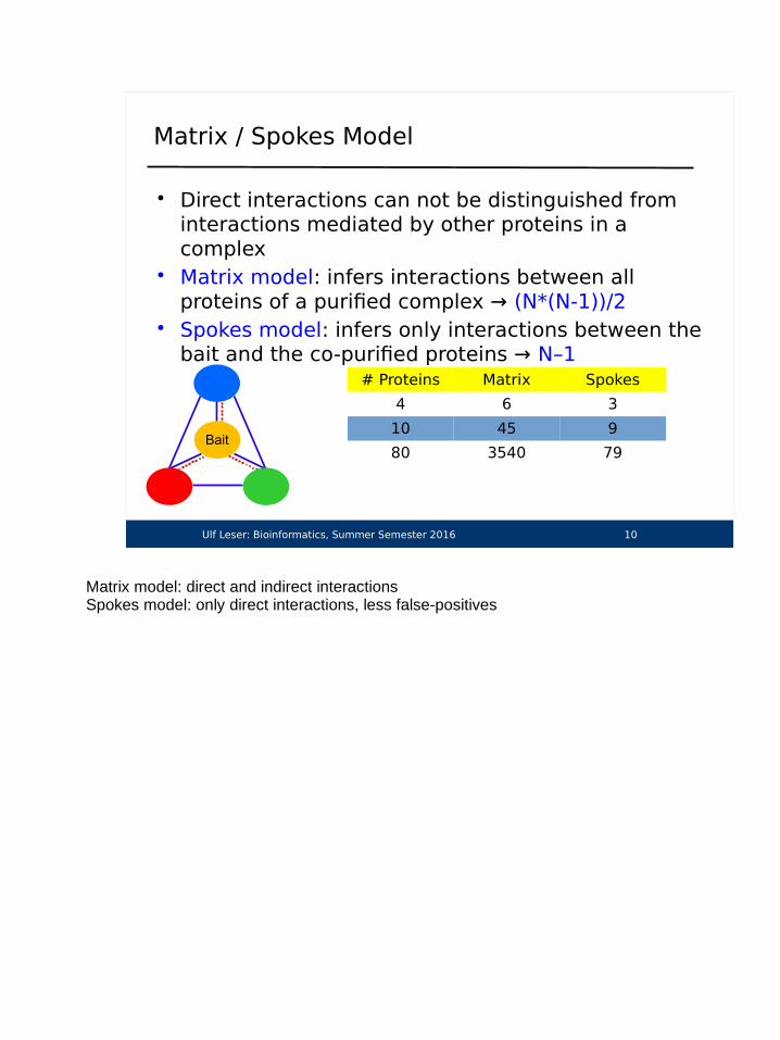
Matrix / Spokes Model
• Direct interactions can not be distinguished from interactions mediated by other proteins in a complex
• Matrix model: infers interactions between all proteins of a purified complex → (N*(N-1))/2
• Spokes model: infers only interactions between the bait and the co-purified proteins → N–1
Bait
# Proteins Matrix Spokes
4 6 3
10 45 9
80 3540 79

Ulf Leser: Bioinformatics, Summer Semester 2016 11
PPI Databases [KP10]
• There are >300 DBs related to PPI and pathways– See http://www.pathguide.org
• Manually curated“source” DBs (blue)– Experimentally
proven interactions– Gather data from
low-throughput methods

Ulf Leser: Bioinformatics, Summer Semester 2016 12
PPI Databases
• There are >300 DBs related to PPI and pathways– See http://www.pathguide.org
• Manually curated“source” DBs
• DBs integrating other DBs and HT data sets (red)

Ulf Leser: Bioinformatics, Summer Semester 2016 13
PPI Databases
• There are >300 DBs related to PPI and pathways– See http://www.pathguide.org
• Manually curated “source” DBs
• DBs integrating othersand HT data sets
• Predicted interactions(yellow)

Ulf Leser: Bioinformatics, Summer Semester 2016 14
PPI Databases
• There are >300 DBs related to PPI and pathways– See http://www.pathguide.org
• Manually curated “source” DBs
• DBs integrating othersand HT data sets
• Predicted interactions• Pathway DBs
(green)
Ulf Leser: Bioinformatics, Summer Semester 2016 15
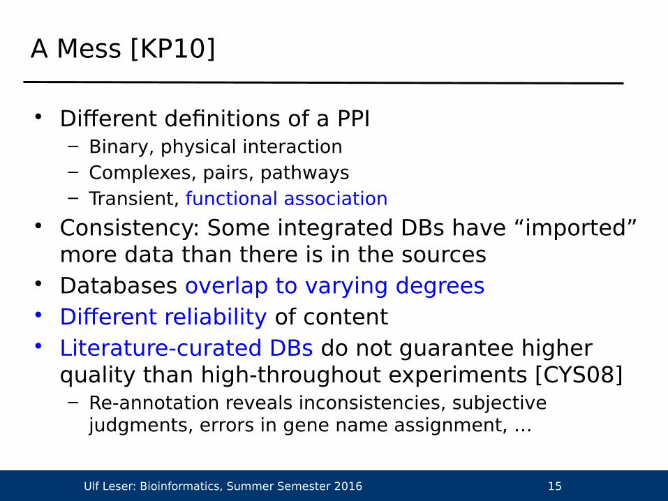
A Mess [KP10]
• Different definitions of a PPI– Binary, physical interaction– Complexes, pairs, pathways– Transient, functional association
• Consistency: Some integrated DBs have “imported” more data than there is in the sources
• Databases overlap to varying degrees• Different reliability of content• Literature-curated DBs do not guarantee higher
quality than high-throughout experiments [CYS08]– Re-annotation reveals inconsistencies, subjective
judgments, errors in gene name assignment, …
Ulf Leser: Bioinformatics, Summer Semester 2016 16
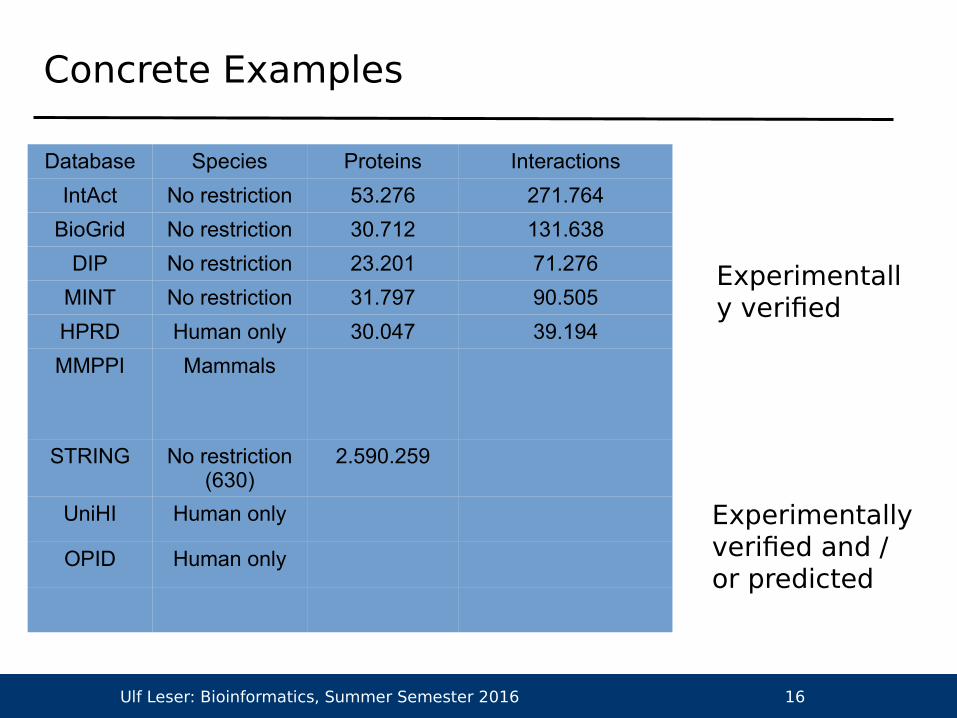
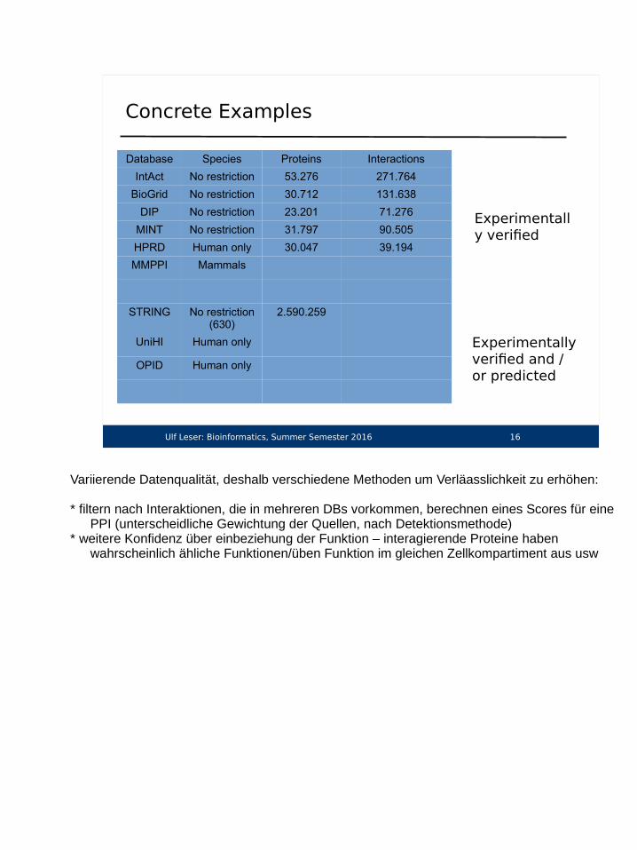
Concrete Examples
Database Species Proteins Interactions
IntAct No restriction 53.276 271.764
BioGrid No restriction 30.712 131.638
DIP No restriction 23.201 71.276
MINT No restriction 31.797 90.505
HPRD Human only 30.047 39.194
MMPPI Mammals
STRING No restriction (630)
2.590.259
UniHI Human only
OPID Human only
Experimentally verified
Experimentally verified and / or predicted

Ulf Leser: Bioinformatics, Summer Semester 2016 17
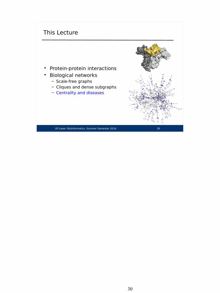
This Lecture
• Protein-protein interactions• Biological networks
– Scale-free graphs– Cliques and dense subgraphs– Centrality and diseases

Ulf Leser: Bioinformatics, Summer Semester 2015 18
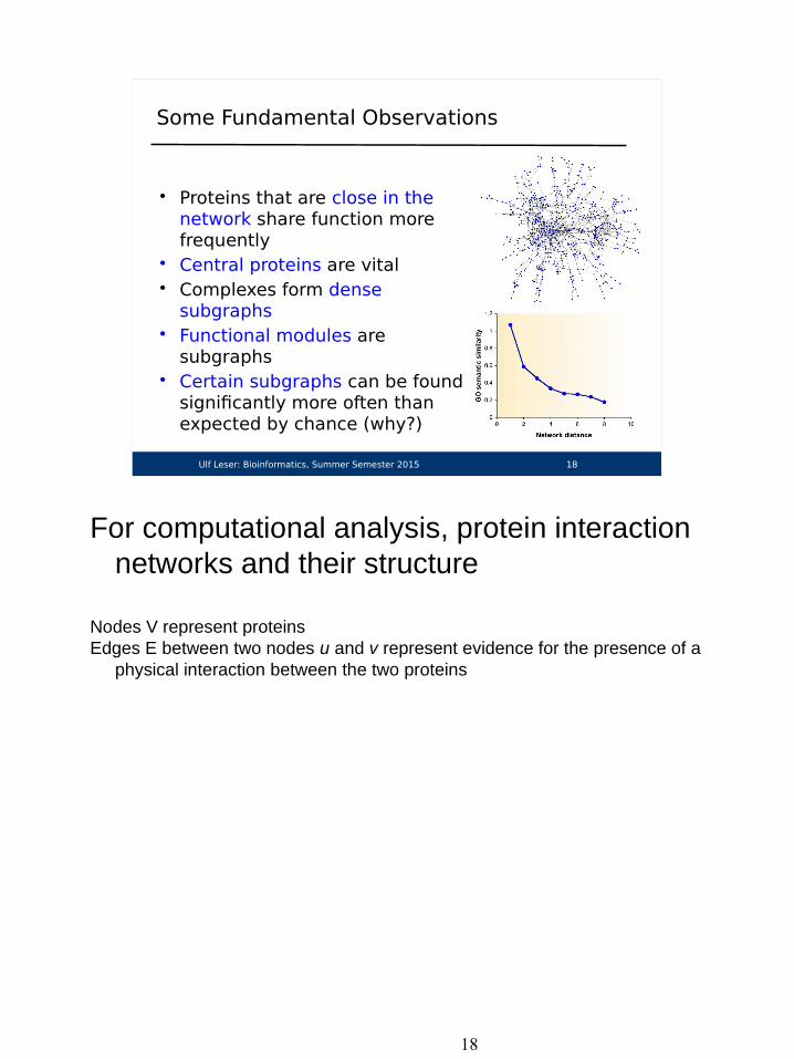
Some Fundamental Observations
• Proteins that are close in thenetwork share function more frequently
• Central proteins are vital• Complexes form dense
subgraphs• Functional modules are
subgraphs• Certain subgraphs can be found
significantly more often than expected by chance (why?)

Ulf Leser: Bioinformatics, Summer Semester 2015 19
Protein-protein interaction networks
• Networks are represented as undirected graphs• Definition of a graph: G = (V,E)
– V is the set of nodes (proteins)– E is the set of binary, undirected edges (interactions)
• Computational representation
B
C
A
D
A B C D
A 0 0 1 1
B 0 0 0 1
C 1 0 0 1
D 1 1 1 0
{ (A,C), (A,D), (B,D), (C,A), (C,D) (D,B) ,
(D,C), (D,A) }
Adjacency matrixAdjacency lists
Ulf Leser: Bioinformatics, Summer Semester 2016 20
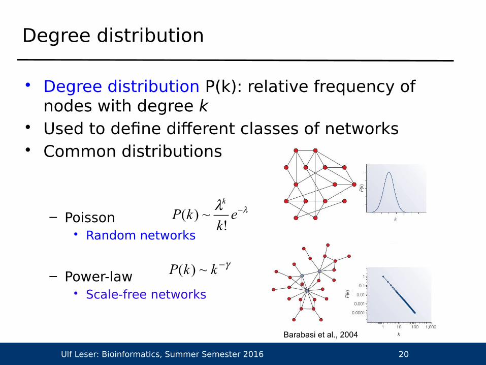
Degree distribution
• Degree distribution P(k): relative frequency of nodes with degree k
• Used to define different classes of networks• Common distributions
– Poisson• Random networks
– Power-law• Scale-free networks
Barabasi et al., 2004
kkP ~)(
ek
kPk
!~)(

Ulf Leser: Bioinformatics, Summer Semester 2016 21
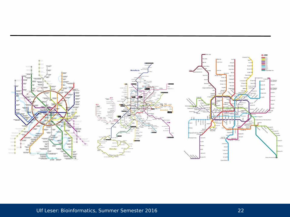
• Biological networks are (presumably)scale-free– Few nodes are highly connected (hubs)– Most nodes have very few connections
• Also true for many other graphs: electricity networks, public transport, social networks, …
• Evolutionary explanation– Growth: Networks grow by addition of new nodes – Preferential attachment: new nodes prefer linking to highly
connec. nodes• Possible explanation: Gene duplication – interaction with same targets
– Older nodes have more chances to connect to nodes– Hub-structure emerges naturally
Scale-free Networks
Ulf Leser: Bioinformatics, Summer Semester 2016 22

Ulf Leser: Bioinformatics, Summer Semester 2016 23
Other Biological Networks
• Regulatory networks: How genes / transcription factors influence the expression of each other– TF regulate expression of genes and of other TFs– Edges semantics: activate / inhibit / regulate– Important, for instance, in cell differentiation
• Signal networks: Molecular reaction to external stimulus– Transient interactions including small molecules– Temporal dimension important (fast)– Important, for instance, in oncology
• Metabolic networks• Protein-protein interaction networks
Ulf Leser: Bioinformatics, Summer Semester 2016 24
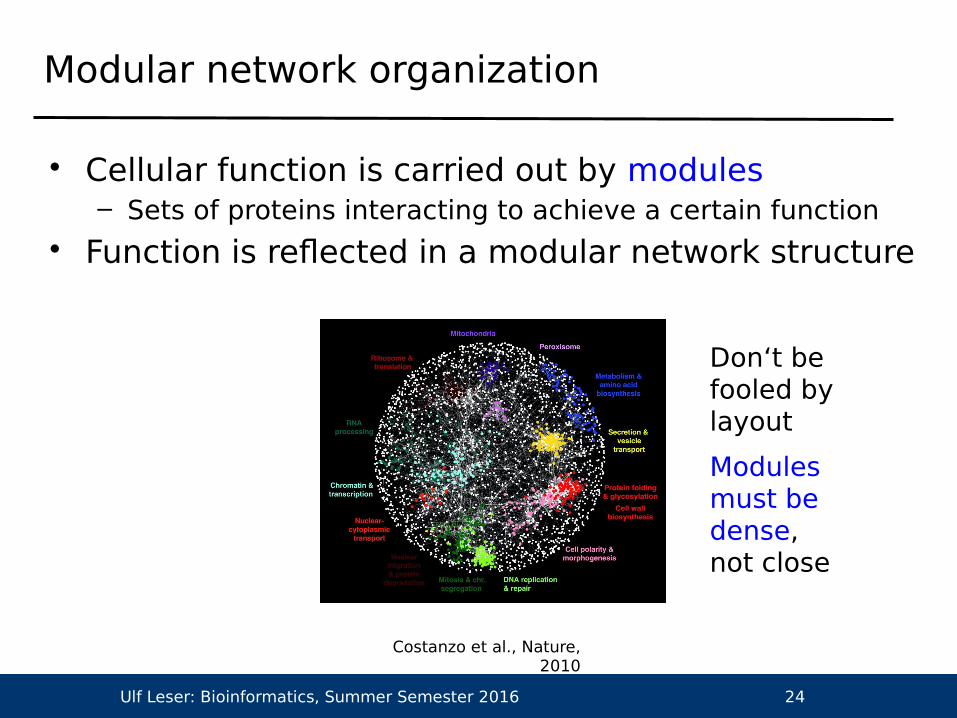
Modular network organization
• Cellular function is carried out by modules – Sets of proteins interacting to achieve a certain function
• Function is reflected in a modular network structure
Costanzo et al., Nature, 2010
Don‘t be fooled by layout
Modules must be dense, not close

Ulf Leser: Bioinformatics, Summer Semester 2016 25
Pathways in cancer
Ribosome subunits – Translation
Proteasome subunits – Protein degradation
Protein transport
MAPK/VEGF/ErbB signaling pathway
Functional Modules

Ulf Leser: Bioinformatics, Summer Semester 2016 26
Clustering Coefficient
• Modules (clusters) are densely connected groups of nodes• Cluster coefficient C reflects network modularity by measuring
tendency of nodes to cluster (‘triangle density’)
– Ev = number of edges between neighbors of v
– dv = number of neighbors of v
– = maximum number of edges between neighbors dv
Vv
vCV
C||
1)1(
2
vv
vv dd
EC
2
)1( vv dd

Ulf Leser: Bioinformatics, Summer Semester 2016 27
Example
v v v
Cv = 10/10 = 1 Cv = 3/10 = 0.3 Cv = 0/10 = 0
• Cluster coefficient C is a measure for the entire graph• We also want to find modules, i.e., regions in the graph with
high cluster coefficient• A clique is a maximal complete subgraph, i.e., a maximal set
of nodes where every pair is connected by an edge

Ulf Leser: Bioinformatics, Summer Semester 2016 28
Finding Modules / Cliques
• Finding all (maximal) cliques in a graph is intractable – NP-complete
• Finding “quasi-cliques” is equally complex– Cliques with some
missing edges– Same as subgraphs
with high clustercoefficient
• Various heuristics– E.g. a good quasi-clique probably contains a (smaller)
clique
build set S2 of all cliques of size 2i:= 2;repeat i := i+1; Si := ; for j := 1 to |Si-1| for k := j+1 to |Si-1| T := Si-1[j] Si-1[k]; if |T|=i-1 then N := Si-1[j] Si-1[k]; if N is a clique then Si := Si N; end if; end if; end for; end for;until |Si| = 0:
Ulf Leser: Bioinformatics, Summer Semester 2016 29
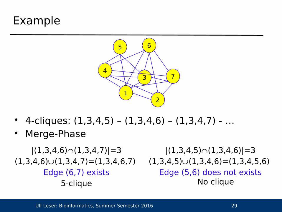
Example
• 4-cliques: (1,3,4,5) – (1,3,4,6) – (1,3,4,7) - … • Merge-Phase
4
1
3
2
7
65
|(1,3,4,6)(1,3,4,7)|=3(1,3,4,6)(1,3,4,7)=(1,3,4,6,7)
Edge (6,7) exists5-clique
|(1,3,4,5)(1,3,4,6)|=3(1,3,4,5)(1,3,4,6)=(1,3,4,5,6)
Edge (5,6) does not existsNo clique

Ulf Leser: Bioinformatics, Summer Semester 2016 30
This Lecture
• Protein-protein interactions• Biological networks
– Scale-free graphs– Cliques and dense subgraphs– Centrality and diseases

Ulf Leser: Bioinformatics, Summer Semester 2016 31
Network centrality
• Central proteins exhibit interesting properties– Essentiality – knock-out is lethal– Much higher evolutionary conservation– Often associated to (certain types of) human diseases
• Various measures exist– Degree centrality: Rank nodes by degree– Betweenness-centrality: Rank nodes by
number of shortest paths between any pair of nodes on which it lies
– Closeness-centrality: Rank nodes by their average distance to all other nodes
– PageRank– …

Ulf Leser: Bioinformatics, Summer Semester 2016 32
Network-based Disease Gene Ranking

Ulf Leser: Bioinformatics, Summer Semester 2016 33
Centrality of Seeds in (OMIM) Disease Networks
Fraction of seeds among top k% proteins; ~600 diseases from OMIM
d1 = direct interactions
d2 = direct and indirect interactions
Rank in % within disease network

Ulf Leser: Bioinformatics, Summer Semester 2016 34
Cross-Validation
• If a disease gene is not yet known – can we find it?
20%
Rank in % within disease network
Cro
ss-v
alid
atio
n re
cove
ry r
ate

Ulf Leser: Bioinformatics, Summer Semester 2016 35
Further Reading
• Jaeger, S. (2012). "Network-based Inference of Protein Function and Disease-Gene Associations". Dissertation, Humboldt-Universität zu Berlin.
• Goh, K. I., Cusick, M. E., Valle, D., Childs, B., Vidal, M. and Barabasi, A. L. (2007). "The human disease network." Proc Natl Acad Sci U S A 104(21): 8685-90.
• Ideker, T. and Sharan, R. (2008). "Protein networks in disease." Genome Res 18(4): 644-52.
• Barabasi, A. L. and Oltvai, Z. N. (2004). "Network biology: understanding the cell's functional organization." Nat Rev Genet 5(2): 101-13.

Protein-Protein-Interaction Networks
Ulf Leser, Samira Jaeger

Ulf Leser: Bioinformatics, Summer Semester 2016 2
This Lecture
• Protein-protein interactions– Characteristics– Experimental detection methods– Databases
• Biological networks
2

Ulf Leser: Bioinformatics, Summer Semester 2016 3
Motivation
• Interaction: Physical binding of two or more proteins– E.g. signal transduction, gene regulation, metabolism, …– Transient or permanent– Directed effect (regulates), undirected (binds), specific
(activates)• Changes in protein structure may hinder bindings and
thus perturb natural cellular processes– Influence on all “downstream” proteins, i.e., proteins
reachable through a path of interactions• Interactome: Set of all PPIs in a cell (type, species, …)• Complex: Permanent binding of two or more proteins
* Interaktion = Wechselwirkung, physikalische Bindung zwischen zwei Proteinen, beruhen meist auf nicht-kovalenten Bindungen wie van-der-Waals Kräfte, Wasserstoffbrücken usw.
* PPI spielen wichtige Rolle bei allen biologischen Prozessen, z.B. Signaltransduktionsprozesse, Metabolismus (Enzyme)
* PPI können permanent (stable) oder transient sein* transient: nur für eine kurzen Effekt kurzzeitig* permanent: Bildung von Multiprotein Komplexen
(zb Cytochrome c)* Arten von Bindungen: gerichtet (Regulation), ungerichtet
(Bindung), spezifisch (Aktivierung)

Ulf Leser: Bioinformatics, Summer Semester 2016 4
Context-dependency
• PPI often is context-dependent– Cell type, cell cycle phase and state– Environmental conditions– Developmental stage– Protein modification– Presence of cofactors and other binding partners– …
• Disregarded by many PPI detection methods• Low quality of typical data sets
4

Ulf Leser: Bioinformatics, Summer Semester 2016 5
Experimental detection methods
• PPIs have been studied extensively using different experimental methods
• Many are small-scale: Two given proteins in a given condition
• High-throughput methods• Yeast two-hybrid assays (Y2H)• Tandem affinity purification and mass spectrometry (TAP-
MS)
Experimentelle Methoden: Protein Microarrays, MS usw
Small scale: less than 100 PPI are considered, typischeerweise mittels X-Ray Kristallographie, Studien beschäftigen sich zumiest mit einem bestimmten Protein
Binary methods: direct physical interactions between proteins (Y2H)Co-compex: direct and indirect interactions (TAP-MS)
Beide sind large-scale
5

Ulf Leser: Bioinformatics, Summer Semester 2016 6
Yeast two-hybrid screens
• Test if protein A (bait) is interacting with B (prey)– Choose a transcription factor T and reporter gene G such
that• If activated T binds to promoter of G, G is expressed • Expression of G can be measured• T can be split in two domains: DNA binding and activation
– Bait is fused to DNA binding domain of T– Prey is fused to activating domain of T– Both are expressed in genetically engineered yeast cells– If A binds to B, T is assembled and G is expressed
Bait protein Prey protein
BDAD
Transcription of reporter gene
Promoter
RNA PolymeraseBD
AD
Hefe-Zwei-Hybrid-System
* testen ob Protein A (bait = Köder) und Protein B (prey = Beute) miteinander interagieren* dabei wird Prinzip der transkriptionellen Aktivierung genutzt
BD: Binding domainAD: Activation domain
* die Voraussetzung für den Test ist das Binden eines TFs an einen Promoter und die darauffolgende Transkription eines downstream liegenden Gens
* Schlüssel: AD und BD funktionieren auch wenn sie nur nahe beieinander sind, sie müssen nicht direkt binden
Samira:- Two fusion protein reconstitute a transcription factor – Bait and prey- utilizes the fact that Transcription Factors commonly require two domains - a DNA binding domain and an activation domain
promoting transcription. In order to find out which proteins interact with a certain protein of interest (termed bait ), the bait is fused to a DNA binding domain which binds to the promoter of a reporter gene, while the other proteins (termed prey) are fused with an activation domain. When a physical interaction between the bait and some
prey occurs, an expression of the reporter gene can be detected.An interaction between a protein containing a DNA binding domain (bait) and an activation domain (prey) can be detected by
measuring the expression level of the reporter gene.
Which proteins interact with protein of interest ?Fuse protein of interest, bait, to DNA binding domainFuse potential binding partners to activation domain
Physical interaction between bait and prey forms an intact functional transcriptional activator → Initiation of the expression of reporter gene
6

Ulf Leser: Bioinformatics, Summer Semester 2016 7
Properties
• Advantages– Throughput: Many preys can be tested with same bait (and
vice versa)– Can be automized – high coverage of interactome– Readout can be very sensitive
• Problems– High rate of false positives (up to 50%)
• Artificial environment: Yeast cells• No post-translational modifications• No protein transport• Unclear if proteins in vivo are ever expressed at the same
time• ...
– Fusion influences binding behavior – false negatives
Vorteile* ermöglicht Untersuchung von PPI in in vivo-ähnlichen Verhältnissen (d.h. im Milieu einer Zelle
und mit in Eukaryoten vorkommenden posttranslationalen Modifikationen, z.B. Glykosylierung, Palmitoylierung)
* Hefe ist relativ billig und leicht zu handhaben
Probleme* Interaktion der untersuchten Proteine muss im Zellkern stattfinden, da dort Trankription
stattfindet. Aber: Proteine falten sich in diesem Milieu ggf.anders als in dem wo sie üblicherweise auftreten
* Modifikationen der Hefe sind teilweise anders als in anderen Eukaryoten (führt zu veränderter Faltung) → insgesamt also falsch-positive Interaktionen möglich: Proteine interagieren nur wegen falscher Faltung miteinander
* auch falsch-negative resultieren daraus: keine Interaktion aufgrund von veränderter Faltung im Kern
* evt. Interaktion im Y2H Versuch, aber in Realität kein gemeinsamen Auftreten im Zellzyklus, Zellorganell oder Zelltyp
nur ca. 50% der mittels Y2H ermittelten Interaktionen sind biologisch bedeutendGroße Anzahl PPI kann mit Y2H nicht detektiert werden

Ulf Leser: Bioinformatics, Summer Semester 2016 8
Tandem affinity purification and mass spectrometry
Bait
1. Tag the protein of interest
4. Purification
5. Purified protein
complexes
6. Identification of associated proteins by
mass spectrometry
2. Protein binds in its natural
environment
3. Complexes are fished by affinity
chromatography
- In a single TAP-MS experiment, a protein of interest, “bait”, is modified by integrating a polypeptide tag into the protein via standard recombinant DNA techniques
- The bait protein is then expressed inside a cell where it may carry out its function as part of one or more protein complexes.
- To retrieve other proteins in a complex, the complex is purified from a cell lysate via affinity chromatography
using the tag of the bait protein. A single experiment is referred to as a purification. - Protein complexes are bound to an IgG column, and washed to remove majority of
contaminants- A single purification is supposed to identify “prey” proteins forming protein
complexes with the baitprotein. - TEV protease is then used to elute the semi-purified protein complexes which are
subsequently absorbed onto a calmodulin column. After further washing, purified protein complexes containing the protein of interest and its associated proteins
- The purified proteins are identified by standard mass spectrometry identification. - Ideally, these purified proteins would constitute the entire complex encompassing
all proteins interactingwith the bait protein.
8

Ulf Leser: Bioinformatics, Summer Semester 2016 9
Properties
• Advantages– Can capture PPI in (almost – the tag) natural conditions– Single bait can detect many interactions in one experiment– Few false positives
• Disadvantages– Tag may hinder PPI – false negatives– Purification and MS are delicate processes– Difficult MS since the input is a mixture of different
proteins– Individual complexes are not identified– Internal structure of complex is not resolved
Vorteile:
Nachteile:* MS/Purification sind anfällige,schwierige Experimente
Ulf Leser: Bioinformatics, Summer Semester 2016 10
Matrix / Spokes Model
• Direct interactions can not be distinguished from interactions mediated by other proteins in a complex
• Matrix model: infers interactions between all proteins of a purified complex → (N*(N-1))/2
• Spokes model: infers only interactions between the bait and the co-purified proteins → N–1
Bait
# Proteins Matrix Spokes
4 6 3
10 45 9
80 3540 79
Matrix model: direct and indirect interactionsSpokes model: only direct interactions, less false-positives

Ulf Leser: Bioinformatics, Summer Semester 2016 11
PPI Databases [KP10]
• There are >300 DBs related to PPI and pathways– See http://www.pathguide.org
• Manually curated“source” DBs (blue)– Experimentally
proven interactions– Gather data from
low-throughput methods
Drei verschiedene Typen von Datenbanken:
* primary databases: containing only experiemnetally proven interactions* enthalten PPI aus small scale experiments* berühmte Beispiele auf Folien:
* BioGRID: Biological General Repository for Interaction datasets* DIP: Database of interacting Proteins* IntAct: molecular interaction database* MNT: molecular interaction database* HPRD: Human Protein Reference Database
* DBs list Spezies, Experiment, Publikation, …* kaum Überlappung zwischen den Datenbanken: in sechs Resourcen gibt es drei PPI, die in
allen Quellen vorkommen, im vergleich sind die Anzahl der Interaktionen, die nur in einer DB vorkommen sehr hoch, zb ~20k in HPRD

Ulf Leser: Bioinformatics, Summer Semester 2016 12
PPI Databases
• There are >300 DBs related to PPI and pathways– See http://www.pathguide.org
• Manually curated“source” DBs
• DBs integrating other DBs and HT data sets (red)
* Wegen der Heterogenität der Daten in den DBs gibt es inzwischen Meta-Dbs, Daten werden kombiniert um zuverlässigere Daten zu erhalten
* nicht einfach: unterschiedliche Ids für Proteine (selbst innerhalb einer DB)

Ulf Leser: Bioinformatics, Summer Semester 2016 13
PPI Databases
• There are >300 DBs related to PPI and pathways– See http://www.pathguide.org
• Manually curated “source” DBs
• DBs integrating othersand HT data sets
• Predicted interactions(yellow)
* kombinieren Daten aus den anderen Datenbanken mit in silico methoden (am computer bestimmt)
* bekannteste: STRING DB* STRING integriert aus versch.Dbs und gewichtet die PPI* methoden um PPI zu predicten:
* aus sequenze Struktur ableiten, ähnliche Domänen die interagieren, interagieren vllt auch zwischen zwei Proteinen mit ähnlichen Domänen* ableitung von homologen Proteinen* co-expression usw.

Ulf Leser: Bioinformatics, Summer Semester 2016 14
PPI Databases
• There are >300 DBs related to PPI and pathways– See http://www.pathguide.org
• Manually curated “source” DBs
• DBs integrating othersand HT data sets
• Predicted interactions• Pathway DBs
(green)

Ulf Leser: Bioinformatics, Summer Semester 2016 15
A Mess [KP10]
• Different definitions of a PPI– Binary, physical interaction– Complexes, pairs, pathways– Transient, functional association
• Consistency: Some integrated DBs have “imported” more data than there is in the sources
• Databases overlap to varying degrees• Different reliability of content• Literature-curated DBs do not guarantee higher
quality than high-throughout experiments [CYS08]– Re-annotation reveals inconsistencies, subjective
judgments, errors in gene name assignment, …
Ulf Leser: Bioinformatics, Summer Semester 2016 16
Concrete Examples
Database Species Proteins Interactions
IntAct No restriction 53.276 271.764
BioGrid No restriction 30.712 131.638
DIP No restriction 23.201 71.276
MINT No restriction 31.797 90.505
HPRD Human only 30.047 39.194
MMPPI Mammals
STRING No restriction (630)
2.590.259
UniHI Human only
OPID Human only
Experimentally verified
Experimentally verified and / or predicted
Variierende Datenqualität, deshalb verschiedene Methoden um Verläasslichkeit zu erhöhen:
* filtern nach Interaktionen, die in mehreren DBs vorkommen, berechnen eines Scores für eine PPI (unterscheidliche Gewichtung der Quellen, nach Detektionsmethode)
* weitere Konfidenz über einbeziehung der Funktion – interagierende Proteine haben wahrscheinlich ähliche Funktionen/üben Funktion im gleichen Zellkompartiment aus usw

Ulf Leser: Bioinformatics, Summer Semester 2016 17
This Lecture
• Protein-protein interactions• Biological networks
– Scale-free graphs– Cliques and dense subgraphs– Centrality and diseases
- Vom Gen zum Protein- mRNA, andere Arten RNA- Kernidee von Microarrays- Affy versus two-color- Populäre chip Typen, kurzer Exkurs neue
Sachen (Exon, tiling)- Probleme mit den Daten- Normalisierung (1-2 Methoden) und
Qualitätssicherung (*wenige*Plotarten mit Kochrezept-artigen Hinweisen)- Technische / biologische Replikate- Wenn möglich was "echtes„
- http://plmimagegallery.bmbolstad.com/
17
Ulf Leser: Bioinformatics, Summer Semester 2015 18
Some Fundamental Observations
• Proteins that are close in thenetwork share function more frequently
• Central proteins are vital• Complexes form dense
subgraphs• Functional modules are
subgraphs• Certain subgraphs can be found
significantly more often than expected by chance (why?)
For computational analysis, protein interaction networks and their structure
Nodes V represent proteinsEdges E between two nodes u and v represent evidence for the presence of a
physical interaction between the two proteins
18

Ulf Leser: Bioinformatics, Summer Semester 2015 19
Protein-protein interaction networks
• Networks are represented as undirected graphs• Definition of a graph: G = (V,E)
– V is the set of nodes (proteins)– E is the set of binary, undirected edges (interactions)
• Computational representation
B
C
A
D
A B C D
A 0 0 1 1
B 0 0 0 1
C 1 0 0 1
D 1 1 1 0
{ (A,C), (A,D), (B,D), (C,A), (C,D) (D,B) ,
(D,C), (D,A) }
Adjacency matrixAdjacency lists
For computational analysis biological networks are modeled as graphs, protein interaction networks and their structure
Nodes V represent proteinsEdges E between two nodes u and v represent evidence for the presence of a
physical interaction between the two proteins
19

Ulf Leser: Bioinformatics, Summer Semester 2016 20
Degree distribution
• Degree distribution P(k): relative frequency of nodes with degree k
• Used to define different classes of networks• Common distributions
– Poisson• Random networks
– Power-law• Scale-free networks
Barabasi et al., 2004
kkP ~)(
ek
kPk
!~)(
* P(k) Wahrscheinlichkeit, dass ein beliebiger Knoten Grad k hat
* number of nodes with degree k N(k) divided by the total number of nodes in the network
* allows to distinguish between different network classes, eg random networks, scale free networks* in a random network the nodes follow a poisson distribution, which indicates that most nodes have approximately the same number of links* random networks: jeder Knoten hat in etwa den gleichen Knotengrad* scale free networks: wenige Knoten haben hohen Knotengrad, viele einen geringen
20

Ulf Leser: Bioinformatics, Summer Semester 2016 21
• Biological networks are (presumably)scale-free– Few nodes are highly connected (hubs)– Most nodes have very few connections
• Also true for many other graphs: electricity networks, public transport, social networks, …
• Evolutionary explanation– Growth: Networks grow by addition of new nodes – Preferential attachment: new nodes prefer linking to highly
connec. nodes• Possible explanation: Gene duplication – interaction with same targets
– Older nodes have more chances to connect to nodes– Hub-structure emerges naturally
Scale-free Networks
* in biological networks gamma is between 2 and 3* highly connected nodes are called hubs* typisch für scale free networks ist, dass es keinen typischen Knotengrad gibt* The smaller gamma, the more important the rate of the hubs in the network* zwei Mechanismen verantwortlich für scale-free Topologien:
* Growth (networks wachsen durch Hinzufügen neuer Knoten)* preferential attachment: nodesae mainly attached to nodes that are already highly connected* gemeinsamer Ursprung: duplikation* duplikation: zwei dientische Gen Produkte entstehen (Growth), außerdem werden duplizierte Gene mit den gleichen Gen Produkten interagieren wie ihr Vorfahr-Gen, da strukturelle Ähnlichkeit
21
Ulf Leser: Bioinformatics, Summer Semester 2016 22
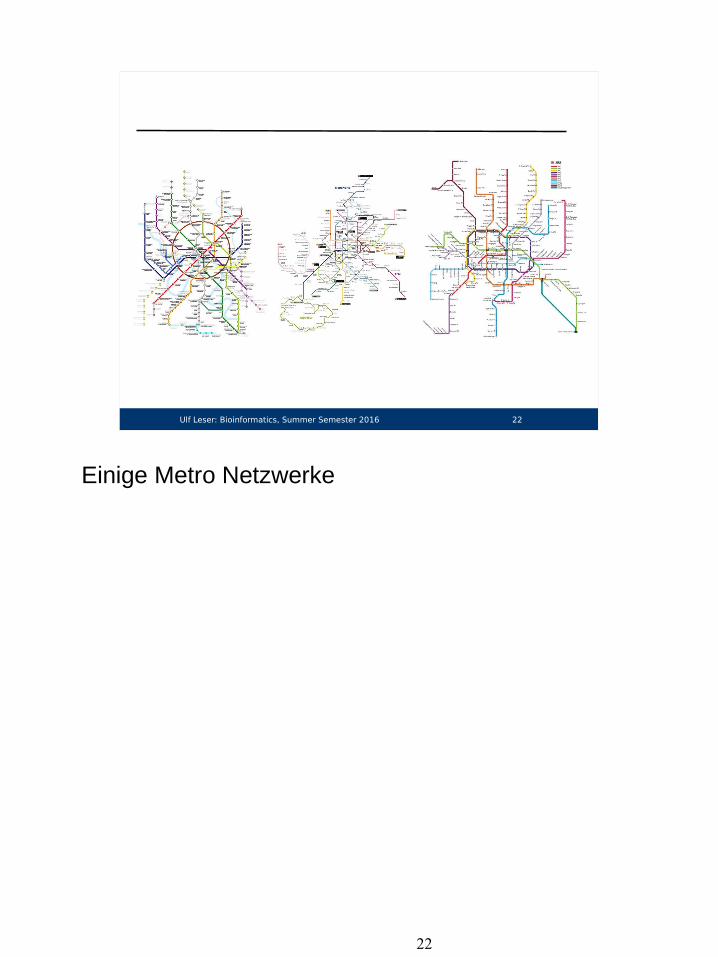
Einige Metro Netzwerke
22

Ulf Leser: Bioinformatics, Summer Semester 2016 23
Other Biological Networks
• Regulatory networks: How genes / transcription factors influence the expression of each other– TF regulate expression of genes and of other TFs– Edges semantics: activate / inhibit / regulate– Important, for instance, in cell differentiation
• Signal networks: Molecular reaction to external stimulus– Transient interactions including small molecules– Temporal dimension important (fast)– Important, for instance, in oncology
• Metabolic networks• Protein-protein interaction networks
Regulatory networks: The activity of genes is regulated by transcription factors, proteins that typically bind to DNA. Most transcription factors bind to multiple binding sites in a genome. As a result, all cells have complex gene regulatory networks. For instance, the human genome encodes on the order of 1,400 DNA-binding transcription factors that regulate the expression of more than 20,000 human genes.[9] Technologies to study gene regulatory networks include ChIP-chip, ChIP-seq, CliP-seq, and others.
Signal networks: Signals are transduced within cells or in between cells and thus form complex signaling networks. For instance, in the MAPK/ERK pathway is transduced from the cell surface to the cell nucleus by a series of protein–protein interactions, phosphorylation reactions, and other events. Signaling networks typically integrate protein–protein interaction networks, gene regulatory networks, and metabolic networks.

Ulf Leser: Bioinformatics, Summer Semester 2016 24
Modular network organization
• Cellular function is carried out by modules – Sets of proteins interacting to achieve a certain function
• Function is reflected in a modular network structure
Costanzo et al., Nature, 2010
Don‘t be fooled by layout
Modules must be dense, not close
This modularity refers to a group of physically or functionally linked molecules/proteins that work together to achieve a (relatively) distinct function
24

Ulf Leser: Bioinformatics, Summer Semester 2016 25
Pathways in cancer
Ribosome subunits – Translation
Proteasome subunits – Protein degradation
Protein transport
MAPK/VEGF/ErbB signaling pathway
Functional Modules

Ulf Leser: Bioinformatics, Summer Semester 2016 26
Clustering Coefficient
• Modules (clusters) are densely connected groups of nodes• Cluster coefficient C reflects network modularity by measuring
tendency of nodes to cluster (‘triangle density’)
– Ev = number of edges between neighbors of v
– dv = number of neighbors of v
– = maximum number of edges between neighbors dv
Vv
vCV
C||
1)1(
2
vv
vv dd
EC
2
)1( vv dd
Der Clusterkoeffizient (engl. clustering coefficient) ist in der Graphentheorie ein Maß für die Cliquenbildung bzw. Transitivität in einem Netzwerk. Sind alle Nachbarn eines Knotens paarweise verbunden, also jeder mit jedem, dann bilden sie eine Clique. Dies ist gleichbedeutend mit dem Begriff der Transitivität, denn innerhalb einer Clique gilt: Ist A mit B verbunden und A mit C, so sind auch B und C verbunden.[1] Man unterscheidet zwischen dem globalen Clusterkoeffizienten, der das gesamte Netzwerk charakterisiert und dem lokalen Clusterkoeffizienten, der einen einzelnen Knoten charakterisiert.
Lokaler CC: Quotient aus der Anzahl der Kanten, die zwischen seinen k_i Nachbarn tatsächlich verlaufen, und der Anzahl Kanten, die zwischen diesen Nachbarn maximal verlaufen könnten (ungerichteter Graph)
Each module can be reduced to a set of triangles – high density of triangles is reflected by a high clustering coefficient
For cliques C = 1For non-triangle graphs = 0
26

Ulf Leser: Bioinformatics, Summer Semester 2016 27
Example
v v v
Cv = 10/10 = 1 Cv = 3/10 = 0.3 Cv = 0/10 = 0
• Cluster coefficient C is a measure for the entire graph• We also want to find modules, i.e., regions in the graph with
high cluster coefficient• A clique is a maximal complete subgraph, i.e., a maximal set
of nodes where every pair is connected by an edge
Each module can be reduced to a set of triangles – high density of triangles is reflected by a high clustering coefficient
For cliques C = 1For non-triangle graphs = 0
27

Ulf Leser: Bioinformatics, Summer Semester 2016 28
Finding Modules / Cliques
• Finding all (maximal) cliques in a graph is intractable – NP-complete
• Finding “quasi-cliques” is equally complex– Cliques with some
missing edges– Same as subgraphs
with high clustercoefficient
• Various heuristics– E.g. a good quasi-clique probably contains a (smaller)
clique
build set S2 of all cliques of size 2i:= 2;repeat i := i+1; Si := ; for j := 1 to |Si-1| for k := j+1 to |Si-1| T := Si-1[j] Si-1[k]; if |T|=i-1 then N := Si-1[j] Si-1[k]; if N is a clique then Si := Si N; end if; end if; end for; end for;until |Si| = 0:
Anderes Beispiel: social network, finden des größten Subset an Leuten, die sich alle kennen

Ulf Leser: Bioinformatics, Summer Semester 2016 29
Example
• 4-cliques: (1,3,4,5) – (1,3,4,6) – (1,3,4,7) - … • Merge-Phase
4
1
3
2
7
65
|(1,3,4,6)(1,3,4,7)|=3(1,3,4,6)(1,3,4,7)=(1,3,4,6,7)
Edge (6,7) exists5-clique
|(1,3,4,5)(1,3,4,6)|=3(1,3,4,5)(1,3,4,6)=(1,3,4,5,6)
Edge (5,6) does not existsNo clique
Ulf Leser: Bioinformatics, Summer Semester 2016 30
This Lecture
• Protein-protein interactions• Biological networks
– Scale-free graphs– Cliques and dense subgraphs– Centrality and diseases
30

Ulf Leser: Bioinformatics, Summer Semester 2016 31
Network centrality
• Central proteins exhibit interesting properties– Essentiality – knock-out is lethal– Much higher evolutionary conservation– Often associated to (certain types of) human diseases
• Various measures exist– Degree centrality: Rank nodes by degree– Betweenness-centrality: Rank nodes by
number of shortest paths between any pair of nodes on which it lies
– Closeness-centrality: Rank nodes by their average distance to all other nodes
– PageRank– …

Ulf Leser: Bioinformatics, Summer Semester 2016 32
Network-based Disease Gene Ranking
-For associating proteins with disease we follow a strategy that is based on finding disease-related proteins according to their similarity to known disease-related genes.-Similarity with disease genes is measured in functional similarity and shared interactions
-For a given disease we first extract all genes that are known to be involved in the disease as seeds-From these seeds we compile a disease specific network by integrating direct and indirctly interacting proteins as well as proteins with functional similarity
• Problem: many (especially novel) genes have little information attached
• Under-annotated genes are under-represented in the network

Ulf Leser: Bioinformatics, Summer Semester 2016 33
Centrality of Seeds in (OMIM) Disease Networks
Fraction of seeds among top k% proteins; ~600 diseases from OMIM
d1 = direct interactions
d2 = direct and indirect interactions
Rank in % within disease network

Ulf Leser: Bioinformatics, Summer Semester 2016 34
Cross-Validation
• If a disease gene is not yet known – can we find it?
20%
Rank in % within disease network
Cro
ss-v
alid
atio
n re
cove
ry r
ate

Ulf Leser: Bioinformatics, Summer Semester 2016 35
Further Reading
• Jaeger, S. (2012). "Network-based Inference of Protein Function and Disease-Gene Associations". Dissertation, Humboldt-Universität zu Berlin.
• Goh, K. I., Cusick, M. E., Valle, D., Childs, B., Vidal, M. and Barabasi, A. L. (2007). "The human disease network." Proc Natl Acad Sci U S A 104(21): 8685-90.
• Ideker, T. and Sharan, R. (2008). "Protein networks in disease." Genome Res 18(4): 644-52.
• Barabasi, A. L. and Oltvai, Z. N. (2004). "Network biology: understanding the cell's functional organization." Nat Rev Genet 5(2): 101-13.