DRAFT

This is a draft version of a conference paper submitted for presentation at UNU-WIDER’s conference, held in Maputo on 5-6 July 2017. This is not a formal publication of UNU-WIDER and may refl ect work-in-progress.

Public economics for development5-6 July 2017 | Maputo, Mozambique

THIS DRAFT IS NOT TO BE CITED, QUOTED OR ATTRIBUTED WITHOUT PERMISSION FROM AUTHOR(S).

WIDER Development Conference

Impact of Fiscal Policy on Inequality and Poverty in Zambia Alejandro de la Fuente,1 Manuel Rosales,2 and Jon Jellema3

June 1, 2017

Abstract. This study assesses the redistributive impact of fiscal policy––and its individual elements––in

Zambia. The team uses fiscal incidence analysis to estimate the distributional effects of fiscal policy in Zambia.

In 2015 Zambia’s fiscal policy reduces inequality. The largest reduction in inequality is created by in-kind public

service expenditures on education.

However, Zambia’s fiscal policy also increases poverty in three ways. (1) It does a relatively low level of

targeted, direct-transfer spending. (2) It makes large expenditures on energy subsidies, which do not reach many

poor households. (3) The tax collection system both through direct and indirect tax instruments creates a burden

greater than the amounts that are received as direct or indirect benefits from subsidies or direct transfers. As a

result, the number of poor and vulnerable individuals who experience net cash subtractions from their incomes

is greater than the number of poor and vulnerable individuals who experience net additions. This dynamic creates

impoverishment among nearly 90 percent of the poor and vulnerable.

Eliminating subsidy spending and moving to directly compensate poorer households would help fiscal policy

achieve poverty reduction and even greater inequality reduction. Because the 2015-era coverage level for the

social cash transfer was low, for many poor households, energy subsidy expenditures delivered their only cash

benefit generated from public expenditures. If subsidies on fuel, electricity, and agricultural inputs were

eliminated entirely without any sizable increase in the SCT program coverage, the impact of fiscal policy on

poverty would likely be muted. Without reform, poor households will also continue to pay more into the fiscal

system than they receive from it in cash.

VAT exemptions reduce the indirect tax burden for all households but cannot eliminate an indirect tax burden

in targeted households. Zambia in 2015 exempted over 80 percent of the average household’s consumption

basket (according to LCMS 2015). However, VAT exemptions imply that some portion of value-added is not

taxed. VAT-exempted items are relatively important consumption-basket items for all households regardless of

income levels. Rather than exempting consumption categories from VAT, a more efficient way to deliver net

benefits to poor and vulnerable households is through targeted cash transfers at a scale large enough to

compensate for the burden created across households by VAT indirect taxes.

JEL Codes: D31, I32

Keywords: Fiscal Policy and Inequality, Income Inequality, Poverty, Social Assistance, Taxation

1 Senior Economist, Poverty and Equity Global Practice, World Bank, 701 18th Street, NW, Washington, DC 20433. Email:

adelafuente@worldbank.org. 2 Senior Economist, African Department, International Monetary Fund, 700 19th Street, NW,

Washington, DC 20433. Email: mrosales@imf.org. 3 Director of Projects, Advisory Services, and Training, Commitment to

Equity Institute, Tulane University. Email: jon.jellema@ceqinstitute.org.

The authors would like to extend sincere thanks to the Central Statistical Office of Zambia (CSO) and the Zambia Revenue

Authority (ZRA) for their support of, and appreciation for, this project. In particular, the team thanks John Kalumbi, Director of

CSO, and Goodson Sinyenga, Deputy Director of Economic and Financial Statistics at CSO, for their support. The authors are also

most grateful to the ZRA team for sharing data and useful inputs, and for their thoughtful comments and advice during the

preparation of the study. In particular, the team thanks Yenda G. Shamabobo, Senior Economist, and Kelvin Mptembamoto,

Assistant Director of Research and Policy at ZRA, for their support. Valuable inputs and comments also were received from CSO

and ZRA during a series of consultations held in Lusaka during early 2017. The authors would also like to thank the following staff

from the World Bank who provided comments and inputs on this report: Ina-Marlene E. Ruthenberg, Andrew Dabalen, Alan Fuchs,

Nadia Belhaj Hassine Belghith, Sebastien Dessus, Cather Signe Tovey, Paolo Belli, Xiaonan Cao, Zivanemoyo Chinzara, Willem

Janssen, Hellen Mbao, Alex Mwanakale, Nicolas Rosemberg, Gregory Smith, Netsanet Walelign, and Emily Weedon. The team

also wishes to thank Alfredo Baldini, IMF Resident Representative in Zambia, for his inputs to the process. The findings,

interpretations, and conclusions in this paper are entirely those of the authors. The findings do not necessarily represent the view

of the World Bank Group, its Executive Directors, or the countries they represent.

1

ABBREVIATIONS

CEQ Commitment to Equity

CIF cost, insurance, and freight

CIT corporate income tax

CSO Central Statistical Office (Zambia)

ECE early child education

FGP Fiscal Gains to the Poor

FI Fiscal Impoverishment

FISP Farmer Input Subsidy Program

GEWEL Girls Empowerment and Women’s Livelihoods Project

kWh kilowatt hour

MoH Ministry of Health

IMF International Monetary Fund

NSSP National Social Protection Policy

PAYE Pay as You Earn (personal income tax)

PER public expenditure review

PIT personal income tax

SADC South African Development Community

SCTS Social Cash Transfer Scheme

SSA Sub-Saharan Africa

VAT value-added tax

WBG World Bank Group

WDI World Development Indicators

WEO World Economic Outlook

WHO World Health Organization

ZESCO Zambian Electricity Corporation

ZMoAL Zambian Ministry of Agriculture and Livestock

2

INTRODUCTION and CONTEXT

The Republic of Zambia is a resource-rich country with massive mineral endowments (especially

copper)4, agricultural potential, and increasingly reliant on construction and other services as a share

of its GDP. The country is geographically large but relatively sparsely populated with a rapidly

growing population (approximately 15.7 million people) (CSO 2016).

In the past decade, Zambia has built on all of these factors to experience robust growth. In the 2000s, after

25 years of decline, per capita incomes improved considerably. In 2011 Zambia returned to lower middle-

income status. Between 2004 and 2014, it recorded impressive economic growth, which averaged 7.6

percent (Smith and others 2016), while Sub-Saharan Africa (SSA) was averaging 5.8 percent (WDI,

multiple years). Between 2004 and 2014, with population growth averaging close to 3.0 percent per annum,

Zambia’s real GDP per capita growth averaged 4.6 percent. During the 25 years, its per capita incomes

improved considerably, moving from US$925 in 1996 to $1,619 (2010 prices) in 2015 (Bhorat and others

2016).

Nevertheless, growth has not brought commensurate improvements in living standards, especially in

rural areas. In 2015 almost 55 percent of the population was living below the national poverty line (Central

Statistical Office 2016). In rural areas, home to the majority of Zambians, the 2015 poverty headcount ratio

exceeded 75 percent. Meanwhile, inequality (as measured by the Gini coefficient of consumption per

capita) in 2015 was 0.56—one of the highest rates globally. This level of inequality represents a significant

increase since 2010, when the Gini coefficient in Zambia hovered approximately 0.52.

Against this background of relatively solid economic growth but with entrenched poverty and

inequality, fiscal policy can directly impact poverty and inequality. This can happen both through the

government’s overall fiscal position – for instance, loose fiscal policy leads to macroeconomic instability

which could lead to higher inflation: the worst tax on the poor– and through the distributional implications

of tax policy and public spending. Experience shows that public spending that is targeted for poor or

vulnerable households may achieve a broader distribution of the benefits of economic growth. For instance,

taxes and transfers have played a significant redistributive role in rich countries and have somewhat

attenuated high inequality (Ravallion 2017).

Poverty reduction policy in Zambia is slowly becoming less growth centered. Previous poverty

reduction policy in Zambia focused on economic growth. Policymakers had shared the view that direct

transfer spending could lead to entitlements and dependency. Noting the limited impact of growth alone,

over the last decade, the government started rolling out unconditional cash transfers via safety net programs

as well as farming input subsidies to smallholders. The government recently also moved toward

withdrawing fuel and electricity subsidies to address current fiscal imbalances while creating fiscal space

for capital spending, addressing large payment arrears, and possibly increasing resources toward social

safety net programs. While allocating public resources, identifying fiscal interventions to help reduce

poverty increasingly has become a concern of the government.

The government’s current fiscal objectives are to address imbalances, including reducing public debt

levels and payment arrears to sustainable levels; and to improve macroeconomic stability. In the

energy sector, reforms will include removing subsidies by moving to full cost-recovery pricing while

maintaining the lifeline to protect the low-income sectors of the population. For electricity, tariff

adjustments are expected to reduce the budgetary burden of public electricity production, distribution, and

subsidization; and attract private investment to boost power supply. For fuel, the government has eliminated

subsidies by moving to full cost recovery. Future fuel prices will adjust to align with cost of future fuel

4 In 2015 Zambia was the second largest copper producer in SSA and the ninth largest in the world.

3

supplies (primarily unrefined fuel). Additionally, the government plans to withdraw from importing

finished products, enabling the oil marketing companies to assume importing them. The Farmer Input

Subsidy Program (FISP) will begin scaling down its coverage (from the current 1.6 million to 1.0 million

farmers) through a “graduation” program.

This study assesses the redistributive impact of fiscal policy, and its individual elements, in Zambia.

The study uses an internationally recognized methodology developed by the Commitment to Equity (CEQ)

Institute. The study estimates the impact of fiscal revenue collections (taxes) and fiscal expenditures––

direct cash and near-cash transfers, in-kind benefits, subsidies––on household-level income inequality and

poverty. It then provides evidence to help policy-makers and other Zambian stakeholders understand the

tradeoffs inherent between government’s current fiscal policy priorities (such as energy policy) and other

social goals (such as poverty reduction). Having an evidence-based understanding of fiscal policy in Zambia

is crucial for two reasons: (1) to inform the government’s ongoing efforts to tackle poverty and (2) to enable

an informed debate among policymakers and with the public while reassessing the scope and design of

existing fiscal instruments to reduce poverty going forward.

The impact of the fiscal system on poverty and inequality in Zambia is described via an estimation of

“pre-fiscal” and “post-fiscal” income measures (Box 1). The pre-fiscal measure comprises market

income before any transfers (including public spending on health and education, farming inputs, fuel and

energy subsidies and unconditional cash transfers) or taxes (including personal income taxes, VAT, alcohol

and tobacco excises) of any kind have been added. “Post-fiscal” income5 takes pre-fiscal income and adds

to it a subset of fiscal policies executed: subsidies and direct transfers received, direct and indirect taxes

paid, and in-kind transfers received through use of services. Poverty and inequality measures then are

derived under pre- and post-fiscal income measures and compared. The primary micro-data source used for

this study is the 2015 Zambian Living Conditions Monitoring Survey assisted by other sources of secondary

data including administrative records.

Zambian fiscal policy, and many of its elements taken individually, reduces income inequality. The

largest reduction in inequality is created by in-kind public service expenditures on education, and the overall

decrease in inequality is more pronounced in rural areas. However, the poverty headcount ratio rises

when fiscal policy is executed. Indirect taxes––most notably, VAT––increase the poverty headcount ratio,

and the direct transfers and subsidies received by poor and vulnerable households are too small to counteract

this impact.6

The study’s results broadly confirm other recent work on the incidence of fiscal policy. Cuesta et al.

(2012) find that neither in-kind education nor health spending nor agricultural input subsidy spending are

strongly pro-poor. The current team also finds, as do Dabalen et al. (2015), that the equitable distribution

of healthcare or education services is driven primarily by demographics and scale effects. In other words,

poor households have more children (on average) creating higher demand for health and education services

5 Post-fiscal income concepts include Net Market Income, Disposable Income, Consumable Income, and Final Income; see Figure

5 and accompanying text below. 6 The apparent contradiction – that one set of fiscal policies can be responsible for a reduction in inequality and an increase in

poverty – can be explained intuitively. The total net gain (or the amount received in benefits minus the amount paid in taxes) is

smaller for richer households, when measured as a percent of their pre-fiscal income, than the total net gain for poorer households

measured as a percent of their pre-fiscal income. Therefore, the post-fiscal income distribution is compressed relative to the pre-

fiscal income distribution and inequality falls. But the net gain from fiscal policy may still be negative or close to zero for all

households. In that case everyone or nearly everyone, including the poor, vulnerable, and the middle class, are measured with

lower levels of post-fiscal income than pre-fiscal income, and poverty rises. This pattern describes the actual distribution of net

fiscal policy gains and losses in Zambia in 2015.

4

in general: and the poor also rely more often on public (rather than private) education and healthcare than

do the rich.7

The rest of this report is organized as follows: Section 2 provides an overview of the main transfers and

taxes in Zambia. Section 3 explains the methodology behind the assessment and a description of the data

sources. Section 4 provides an overview of the main findings from the Zambia assessment with international

benchmark comparisons. Section 5 concludes by spelling out the implications of the results for policy in

Zambia.

PRIMER ON SOCIAL SPENDING AND TAXES IN ZAMBIA

The fiscal system in Zambia comprises a set of social expenditures and taxes. On the expenditure side,

benefits include public spending on health and education. In recent years, the country also has relied on

farming inputs and fuel and energy subsidies. A nascent system of social protection is in the making, mainly

through unconditional cash transfers. On the tax side, instruments include personal income taxes, VAT, and

alcohol and tobacco excises. Section 2 gives an overview of the size and composition of each of these main

fiscal tools.8

Social Spending and Transfers

Social spending in Zambia can be divided in three categories: in-kind transfers, direct transfers, and

subsidies. Table 1 provides a snapshot of these (and other) expenditures in fiscal year 2015.9 Social

expenditures––social protection, education, heath, and housing and urban spending––account for over 25

percent of total expenditures. Subsidy spending accounts for approximately 5 percent, infrastructure for just

over 10 percent, and defense and law and order for approximately 5 percent. Other sectors, such as Energy

and Mineral Development, Information and Communications Technology, Tourism, Trade, and Industry,

account for the remaining approximately 50 percent.

Table 1 provides a snapshot of the fiscal expenditures covered by this assessment. Defense spending

and Infrastructure are not covered, but most of the Social Protection portfolio is incorporated. The public

service pension fund is included, but, for reasons explained below, the study treats these expenditures as

part of the public sector or civil service wage bill rather than as a tax and transfer program.

Table 1. Zambia government expenditures, 2015

Expenditures Included

in

analysis? Kwacha

(billions)

GDP

(%)

Total expenditure 51.7 28.1

Social Spending 14.7 8.0

Social Protection 0.8 0.5

Social Assistance of which 0.2 0.08

Conditional or Unconditional Cash

Transfers

0.2 0.08 Yes

7 Therefore, education and health spending is equitable not from a policy design standpoint. In reality, higher-valued public health

and education services (like hospital-based care or university education) are more frequently accessed by richer households, which

creates a regressive distribution of the value of publicly-delivered services at some service levels or types. 8 The IMF notes that compensation to employees (civil servants) (at 50% of government revenues), subsidies (at 30%), and debt

service absorb over 100% of the budget’s ordinary revenues, thus limiting operational and other spending including social cash

transfers and public investment. (Zambia: Towards Achieving Fiscal Sustainability. Selected Issues Paper, forthcoming). 9 Zambia’s fiscal year is January 1–December 31.

5

Noncontributory Pensions --

Near-cash Transfers --

Other --

Social Insurance of which

Public Service Pension Fund 0.8 0.44 Yes

Education of which 9.4 5.1

Pre-school -- No

Primary -- Yes

Secondary -- Yes

Post-secondary non-tertiary No

Tertiary -- Yes

Health of which 4.5 2.4 Yes

Contributory

Noncontributory

Housing and Urban -- --

Subsidies of which 4.2 2.3

Energy of which 3.1 1.7

Electricity 0.4 0.2 Yes

Fuel 2.7 1.5 Yes

Food -- --

Agricultural Inputs 1.1 0.6 Yes

Water -- --

Infrastructure of which 6.2 0.0

Water and Sanitation 0.5 0.3 No

Rural Electrification 0.1 0.0 No

Rural Roads 5.6 3.0 No

Defense; Public Order; Safety Spending 3.2 1.8 No

Other 24.4 13.3 No

Source: Republic of Zambia Annual 2015 Economic Report (2016)

http://www.mof.gov.zm/index.php/publicfinancialmanagement/summary/91-detailed-annual-financial-reports/15046-financial-

report-2014-detailed and Republic of Zambia 2016 Budget Address, both from the Ministry of Finance.

http://www.mof.gov.zm/index.php/budgetdata/summary/15-budget-speeches/9751-budget-speech-2016

Note: Expenditures (and revenues) included may not be fully allocated within LCMS 2015 for various reasons. See sec. 3 for allocative methods and assumptions.

Some public expenditure elements have private analogues: for example, individuals who do not belong to

the public contributory pension system may contribute and receive income from a private pension fund.

Though such privately-arranged goods and services are included in measures of income, we do not attempt

to determine their impact on welfare or inequality as they are not part of the fiscal system. Other public

expenditure elements are part of the fiscal system but cannot be allocated because of data limitations. For

example, the household survey may not record who utilizes post-secondary, non-tertiary education or

available budget reporting may not have a separate entry for post-secondary, non-tertiary education

expenditures (or both limitations may be present).

6

In-Kind Transfers

Education

Education has remained a priority for Zambia. Between 2006 and 2013, the proportion of public

expenditure on education in total government expenditure was 15 percent–21 percent (equivalent to 3.7

percent–4.4 percent of GDP). In in 2014 and 2015, in real terms, public expenditure on education has

increased to over 5 percent of GDP. In the 2015 proposed budget, education is the largest single-sector

allocation, putting Zambia in the top 33 percent of Sub-Saharan African countries ranked by public

education expenditure as a share of GDP (World Bank 2015).

Enrollment at all levels continues to rise. Zambia’s public education system is organized according to

four levels: early child education (ECE) for preprimary school children; primary education (grades 1–7) for

children ages 7–14; secondary education (grades 8–12) for children ages 15–19, and tertiary (college and

university degree programs). “Basic” education consists of 9 years of education: 6 at the primary level and

3 at the secondary level. Since 2000, student enrollment has been increasing at all levels. Between 2009

and 2013, enrollment at higher education and secondary school levels increased substantially (48 percent).

The enrollment increase in secondary education reflects the growing number of graduates at the primary

education level. Similarly, the recent rapid growth of higher education enrollment is due mainly to the

increasing number of graduates from secondary education and probably due also to more students aspiring

to higher education. A 2014 study showed that almost 90 percent of primary and secondary students want

to pursue at least a bachelor’s degree in higher education.

In 2014 and 2015, the focus of education expenditure began to shift gradually from basic to secondary

and higher education, with increased capital outlays for those levels. Non-administrative expenditures are

highest at the primary education level. Between 2006 and 2013, per-student public expenditures at the

primary level saw a large increase (in nominal terms). Nonetheless, in 2013 public expenditure per student

at the high school level (grades 10–12) was 2.7 times larger than the same amount at the basic school level

(grades 1– 9), while expenditure per student at the university level was over 15 times larger than that at the

basic school level. Although a “free” primary education policy was introduced in 2002, students continue

to pay out-of-pocket fees. This reality further reduces the value of the in-kind transfer for primary education

provided via government expenditure. At the other end of the education spectrum, a relatively generous

bursary program subsidizes the cost of textbooks and other supplies for public university students who

come primarily from relatively wealthy households.

Private expenditures by poor households on public education can be traced partly to weak public

expenditure execution. For example, 30 percent of primary schools do not receive the government grants

that support the free education policy on time so end up collecting fees from students to cover the shortfall.

Likewise, by law, the bursary scheme is a loan/financing scheme––but the program lacks a loan collection

mechanism. These monies could be self-sustaining (instead of an adding annual budgetary burden), and the

current budget transfer that they require could be redirected toward pro-poor education spending. However,

at present, the scheme’s implementation constraints preclude this possibility.

Health

During the last decade, Zambia expanded its health investments. Zambia’s annual per capita total health

expenditure increased from US$26.50 in 2003 to $86.00 in 2014.10 The latter is equivalent to the

recommended US$86 per capita per annum (in 2012 constant dollars) for low-income countries (though

10 Government expenditures on health account for over 50% (US$48) of the total; the rest (US$38) is paid by donors, households,

employers. Figures come from the WHO Global Health Expenditure database: http://apps.who.int/nha/database.

7

Zambia recently moved into low-middle income status) to have a fully functioning health system (McIntyre

and Meheus 2014) ; and doubles the US$43 per capita that Zambia’s peers spend on health.

Between 2011 and 2015, the government’s nominal health budget increased by 135 percent, but expenditure

execution makes it difficult to efficiently provide the necessary high-quality services. For example, only 67

percent of the money allocated to districts in 2013 (and 201611) was disbursed (MoH 2016). In 2015

government health expenditures are skewed toward salaries and wages, which represent 59 percent of the

total government health budget and 85 percent of funds allocated to districts for health expenditures. This

rate is above the 40 percent historical average for African countries and 45 percent average for high-income

countries (Vujicic and others 2009).

Zambian health transfers are made through three levels of service provision. The first level consists

of local care provided at district hospitals, clinics, and ward-level health posts. The second level is populated

by the larger, better-staffed provincial general hospitals that provide direct and referral care. The third level

comprises national and specialized hospitals that focus on complicated procedures and rare conditions. In

practice, just over 33 percent of total health spending is allocated to the first service level, of which amount

nonpersonnel health spending takes up approximately 20 percent. While user fees charged by primary

providers were abolished between 2006 and 2011, the extent of fees and charges levied by public providers

of healthcare is unknown. For example, not all areas are served equally well by the drug and medical

supply distribution system so the total cost of a primary provider visit is not always zero or near zero.

Direct Transfers

In 2014, the Government of Zambia approved the National Social Protection Policy (NSSP). The

policy is intended to provide for “the well-being of all Zambians by ensuring that vulnerable people have

sufficient income security to meet basic needs and protection from worst impacts of risks and shocks.”

Toward this objective, the government organized its noncontributory programs (those typically tailored to

the poor and vulnerable) around the two pillars of social assistance and livelihoods and empowerment, as

well as a cross-cutting focus on disability in government programs. The largest programs within these areas

are the Social Cash Transfer Scheme (SCTS), the Farmer Input Support Program (FISP) and the Food

Security Pack, and the Girls Empowerment and Women’s Livelihoods (GEWEL) Project. In the incidence

analysis that follows, the team includes SCTS (as a direct transfer) and FISP (as a subsidy scheme). In 2015

GEWEL was known as the Woman’s Development Programme. Both coverage and public expenditures on

the program were minimal so the team does not include it.

Social Cash Transfer (SCT)

SCTS is the government’s flagship social assistance program. It targets poor households that include

one or more disabled members and poor and vulnerable individuals for regular consumption support

through an unconditional cash transfer. SCTS employs both a proxy means test and categorical targeting as

well as community-level advice concerning potential beneficiaries. Since its introduction in 2003, STCS

has been scaling up gradually. In 2011 the program covered approximately 33,000 of the poorest households

with monthly transfers of Kwacha 70 for households without disabled members, and Kwacha 140 for

households with disabled members (approximately $US7–14, respectively). By 2015 over 150,000 SCTS

beneficiaries could be found in approximately 50 percent of the country’s 103 districts (Republic of Zambia,

2016). In 2017 the government expects to cover 500,000 beneficiaries (Republic of Zambia, 2016) in all

103 districts with an increase in the monthly transfer amount to Kwacha 90 (approximately $9).

11 A review of budget performance in 2016 shows that 67% of allocated funds (at district level, and tertiary and secondary level

hospitals) was released January 1–October 3.

8

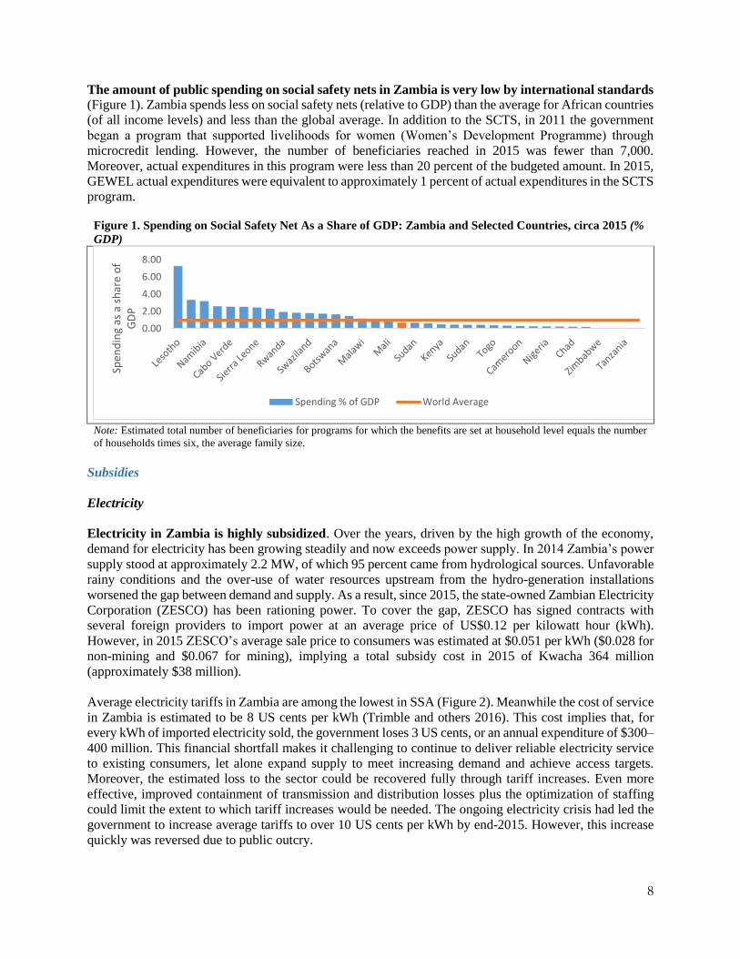
The amount of public spending on social safety nets in Zambia is very low by international standards

(Figure 1). Zambia spends less on social safety nets (relative to GDP) than the average for African countries

(of all income levels) and less than the global average. In addition to the SCTS, in 2011 the government

began a program that supported livelihoods for women (Women’s Development Programme) through

microcredit lending. However, the number of beneficiaries reached in 2015 was fewer than 7,000.

Moreover, actual expenditures in this program were less than 20 percent of the budgeted amount. In 2015,

GEWEL actual expenditures were equivalent to approximately 1 percent of actual expenditures in the SCTS

program.

Figure 1. Spending on Social Safety Net As a Share of GDP: Zambia and Selected Countries, circa 2015 (%

GDP)

Note: Estimated total number of beneficiaries for programs for which the benefits are set at household level equals the number

of households times six, the average family size.

Subsidies

Electricity

Electricity in Zambia is highly subsidized. Over the years, driven by the high growth of the economy,

demand for electricity has been growing steadily and now exceeds power supply. In 2014 Zambia’s power

supply stood at approximately 2.2 MW, of which 95 percent came from hydrological sources. Unfavorable

rainy conditions and the over-use of water resources upstream from the hydro-generation installations

worsened the gap between demand and supply. As a result, since 2015, the state-owned Zambian Electricity

Corporation (ZESCO) has been rationing power. To cover the gap, ZESCO has signed contracts with

several foreign providers to import power at an average price of US$0.12 per kilowatt hour (kWh).

However, in 2015 ZESCO’s average sale price to consumers was estimated at $0.051 per kWh ($0.028 for

non-mining and $0.067 for mining), implying a total subsidy cost in 2015 of Kwacha 364 million

(approximately $38 million).

Average electricity tariffs in Zambia are among the lowest in SSA (Figure 2). Meanwhile the cost of service

in Zambia is estimated to be 8 US cents per kWh (Trimble and others 2016). This cost implies that, for

every kWh of imported electricity sold, the government loses 3 US cents, or an annual expenditure of $300–

400 million. This financial shortfall makes it challenging to continue to deliver reliable electricity service

to existing consumers, let alone expand supply to meet increasing demand and achieve access targets.

Moreover, the estimated loss to the sector could be recovered fully through tariff increases. Even more

effective, improved containment of transmission and distribution losses plus the optimization of staffing

could limit the extent to which tariff increases would be needed. The ongoing electricity crisis had led the

government to increase average tariffs to over 10 US cents per kWh by end-2015. However, this increase

quickly was reversed due to public outcry.

0.00

2.00

4.00

6.00

8.00

Spen

din

g as

a s

har

e o

f G

DP

Spending % of GDP World Average

9

Figure 2. Electricity Tariffs in Sub-Saharan Africa (US$/kWh)

Source: Trimble et al. 2016.

Note: Constant 2014 US$ per kWh sold, excluding VAT.

Fuels

Zambia imports fuel, and the government handles all procurement. The bulk of the unprocessed

feedstock imports traditionally are brought to the state-owned Indeni refinery (via the state-owned Tazama

pipeline), in which they are refined to obtain the final market mix.12 In recent years, imports of refined

products, also procured by the government, gradually have increased and now represent approximately 50

percent of total fuel imports. These fuels are being imported directly by road. Retail prices set by the

government do not adjust automatically to input price changes or production costs. Consequently, as market

prices for fuel increase and the Zambian Kwacha loses value, for example, against other trading currencies,

fuel subsidies have become the norm. The financing gap is covered directly by an on-budget transfer. This

implicit fuel subsidy cost the government approximately $500 million in 2015.

Managed retail prices do not systematically adjust to reflect actual costs; therefore implicit fuel

subsidies are the norm. From early 2010 to mid-2014, retail prices in kwacha rose by close to 60 percent

for both petrol and diesel. In contrast, during the same period, measured in US dollars, the price increases

were lower at just under 20 percent, approximately only half of the almost 40 percent increase in the price

of crude oil. In the second half of 2014, the drop in international oil prices lowered the cost-reflective price

below the retail price for some shipments. In January 2015, retail prices were reduced by 20 percent which

brought retail prices again under the cost-reflective price.13

Farmer Input Support Program (FISP)

In 2002–03, the Government of Zambia introduced the Farmer Input Support Program (FISP). Its purpose

is to improve the supply and delivery of fertilizer and seeds for maize production14 at subsidized prices to

12 A blend of crude oil, condensate, naphtha, and gasoil (diesel). 13 Retail prices increases of 9 percent and 15 percent were approved in May and July 2015, respectively, but these increases did

not bring the retail price to or above the cost-reflective price.

14 In the early years of the program (2002/03–2008/09), participating farmers received 400 kg of fertilizer (200 kg each of

compound D and urea), and 20 kg of hybrid maize seed at a 50% subsidy. From 2009/10 on, the input pack size was halved to 200

kg of fertilizer and 10 kg of hybrid maize seed. In 2010/11, small quantities of rice seed were added to the program; and in 2011/12,

sorghum, cotton, and groundnut seed were added. In 2014/15 cottonseed was dropped, and the groundnut seed quantity increased

more than 10-fold. Subsidy rates have varied over time, ranging from 50%–79% for fertilizer, and 50%–100% for seed.

0.05

0.00

0.10

0.20

0.30

0.40

0.50

0.60

0.70

Eth

iop

ia

Sud

an

Zam

bia

Leso

tho

Sou

th A

fric

a

Mo

zam

biq

ue

Co

ngo

, Rep

.

Zim

bab

we

Gh

ana

Gu

ine

a

Cam

ero

on

Ken

ya

Uga

nd

a

Mal

i

Gab

on

Co

mo

ros

Rw

and

a

Sen

egal

Sier

ra L

eon

e

Lib

eri

a

10

farmers who cultivate less than 5 hectares of land15 to increase their household food security and incomes

through increased productivity. These inputs are procured at market prices by the government and then sold

below cost through the farmer cooperative system.

To qualify for FISP support, farmers need to belong to a cooperative or farmer association and have the

capacity to grow one hectare of maize. Land-constrained households (who are mostly poor households)

cannot access these inputs. Sometimes smallholders do not belong to cooperatives, so it is more often

relatively large farmers who can access the subsidized inputs, even though the objectives of the input

programs are to support the “vulnerable but viable” smallholder farmers in Zambia (Mason and others

2013).16 Its targeting criteria require the capacity to grow between 0.5 and 5.0 hectares of maize, which

already excludes the poorest and landless households.

FISP was envisaged as a temporary program to be phased out after three years. Instead, over the last

13 years, it has grown in scale and budget to the point of becoming one of Zambia’s two major agricultural

sector poverty reduction programs, the other being the Food Reserve Agency, a maize marketing board and

strategic food reserve. FISP began with a budget of US$22 million, but by 2015, the budget allocation was

$217 million, by far Zambia’s largest transfer program (also in number of beneficiaries). During the last 5

years, except for the 2012–13 season, FISP has reached more than 400,000 households per year. Despite

crowding out other public investments in agriculture, FISA could make a dent in poverty by making

available key inputs to a large population of poor farmers and potentially raise their productivity. However,

FISP access requires certain characteristics that exclude many poor households leading to a greater

concentration of FISP resources among non-poor households.

The effects of FISP on maize yields and consumer prices have been modest. Participation raises

production by 188 kilograms of maize for every 100 kilograms of FISP fertilizer, which is considerably

less than in Kenya, for example, where participation in a similar scheme (NAAIAP17) raises maize

production by an average of 361 kilograms (Mason and others 2015). FISP has had similarly modest effects

on reducing food prices: the available evidence for Zambia suggests modest reductions in retail maize

prices18 on the order of 1 to 4 percent (Ricker-Gilbert et al. 2013; Arndt et al. 2014).

Inefficiencies in program implementation explain part of FISPs’ impact on production. A study in the

2007–08 season found serious problems with late delivery: less than 4 percent of beneficiaries said they

received their inputs by the end of October when planting starts, and 69 percent said they did not get their

inputs until after the start of the rains. The same study discovered that only 44 percent of farmers actually

received the full fertilizer allowance which affected farmers’ production decisions.

15 Based on the 2014/15 official eligibility criteria, targeted beneficiaries were to be: (i) small-scale farmers (that is, cultivating

less than 5 ha of land); registered with the Ministry of Agriculture and Livestock (ZMoAL) and actively engaged in farming; (ii)

members of a farmer organization that had been selected to participate in FISP; and (iii) not concurrent beneficiaries of the Food

Security Pack Programme. The targeted beneficiaries also needed to have the financial means to pay the farmer share of the input

costs (for example, in 2014/15, approximately US$65 total for 200 kg of fertilizer and 10 kg of hybrid maize seed). In previous

years, the program also required that beneficiaries have the capacity to cultivate a minimum area of land (for example, 1 ha in

2012/13) (ZMoAL 2012).

16 Households with 2–5 ha of land make up 21% of the country’s poor smallholders. Nevertheless, they received 41% of the

fertilizer distributed through the program. In contrast, despite being 26% of the country’s poor smallholders and 24% of all

households, households with 0.5–1.0 ha received only 13% of the subsidies.

17 Receipt of 100 kg of fertilizer and 10 kg of improved maize seed if a household obtains a full input pack.

18 Lowering food prices could benefit urban consumers and net food buyers in rural areas, who make up over 33 percent of

households.

11

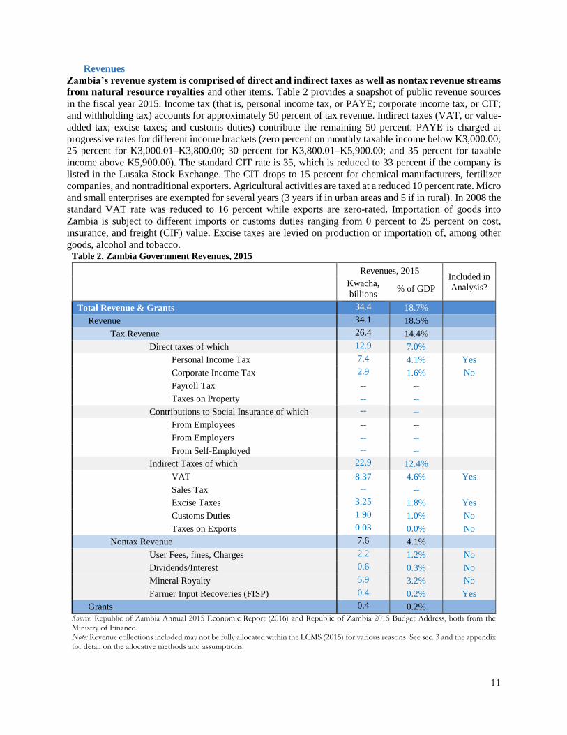
Revenues

Zambia’s revenue system is comprised of direct and indirect taxes as well as nontax revenue streams

from natural resource royalties and other items. Table 2 provides a snapshot of public revenue sources

in the fiscal year 2015. Income tax (that is, personal income tax, or PAYE; corporate income tax, or CIT;

and withholding tax) accounts for approximately 50 percent of tax revenue. Indirect taxes (VAT, or value-

added tax; excise taxes; and customs duties) contribute the remaining 50 percent. PAYE is charged at

progressive rates for different income brackets (zero percent on monthly taxable income below K3,000.00;

25 percent for K3,000.01–K3,800.00; 30 percent for K3,800.01–K5,900.00; and 35 percent for taxable

income above K5,900.00). The standard CIT rate is 35, which is reduced to 33 percent if the company is

listed in the Lusaka Stock Exchange. The CIT drops to 15 percent for chemical manufacturers, fertilizer

companies, and nontraditional exporters. Agricultural activities are taxed at a reduced 10 percent rate. Micro

and small enterprises are exempted for several years (3 years if in urban areas and 5 if in rural). In 2008 the

standard VAT rate was reduced to 16 percent while exports are zero-rated. Importation of goods into

Zambia is subject to different imports or customs duties ranging from 0 percent to 25 percent on cost,

insurance, and freight (CIF) value. Excise taxes are levied on production or importation of, among other

goods, alcohol and tobacco. Table 2. Zambia Government Revenues, 2015

Revenues, 2015 Included in

Analysis? Kwacha,

billions % of GDP

Total Revenue & Grants 34.4 18.7%

Revenue 34.1 18.5%

Tax Revenue 26.4 14.4%

Direct taxes of which 12.9 7.0%

Personal Income Tax 7.4 4.1% Yes

Corporate Income Tax 2.9 1.6% No

Payroll Tax -- --

Taxes on Property -- --

Contributions to Social Insurance of which -- --

From Employees -- --

From Employers -- --

From Self-Employed -- --

Indirect Taxes of which 22.9 12.4%

VAT 8.37 4.6% Yes

Sales Tax -- --

Excise Taxes 3.25 1.8% Yes

Customs Duties 1.90 1.0% No

Taxes on Exports 0.03 0.0% No

Nontax Revenue 7.6 4.1%

User Fees, fines, Charges 2.2 1.2% No

Dividends/Interest 0.6 0.3% No

Mineral Royalty 5.9 3.2% No

Farmer Input Recoveries (FISP) 0.4 0.2% Yes

Grants 0.4 0.2%

Source: Republic of Zambia Annual 2015 Economic Report (2016) and Republic of Zambia 2015 Budget Address, both from the Ministry of Finance. Note: Revenue collections included may not be fully allocated within the LCMS (2015) for various reasons. See sec. 3 and the appendix for detail on the allocative methods and assumptions.

12

At approximately 14 percent of GDP, Zambia’s tax ratio is low. The taxable base is eroded by a significant

list of exemptions. For example, value-added tax (VAT) exemptions include domestic kerosene, health,

education, domestic house rentals, water, transport, financial and life insurance services, and food and

agriculture, among others; books are zero-rated. VAT’s efficiency rate is defined as the actual, confirmed

VAT revenue raised relative to the value of consumption for each percentage point of the statutory VAT

rate, or the effective VAT rate (over all consumption) relative to the statutory rate. Against the background

of Zambia’s exemptions, the VAT efficiency rate is quite low, averaging 21 percent during 2008–12. The

efficiency rate increased to 36 percent in 2014 but in 2015 fell back to 28 percent.19 Zambia’s personal

income tax, the Pay-As-You-Earn (PAYE) tax, has a high threshold, and several income components (such

as capital gains) are excluded from the base. The base for the corporate income tax is limited by widespread

exemptions and multiple tax rates. Zambia does not have a property tax.

This study covers the majority of indirect taxes and the personal income tax. The team has information

on Zambia’s personal income tax (PAYE). However, the team does not have enough information to allocate

CIT burdens to households in the micro-dataset nor enough administrative information to allocate Social

Insurance contributions.

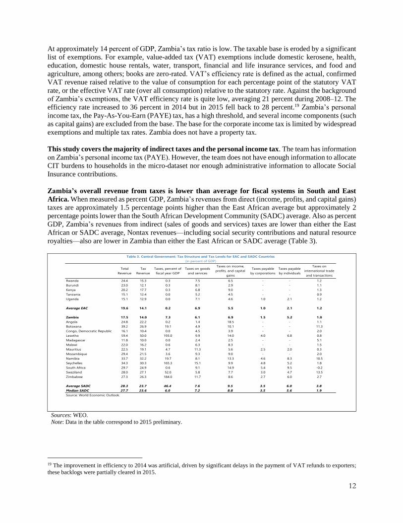
Zambia’s overall revenue from taxes is lower than average for fiscal systems in South and East

Africa. When measured as percent GDP, Zambia’s revenues from direct (income, profits, and capital gains)

taxes are approximately 1.5 percentage points higher than the East African average but approximately 2

percentage points lower than the South African Development Community (SADC) average. Also as percent

GDP, Zambia’s revenues from indirect (sales of goods and services) taxes are lower than either the East

African or SADC average, Nontax revenues––including social security contributions and natural resource

royalties––also are lower in Zambia than either the East African or SADC average (Table 3).

Sources: WEO.

Note: Data in the table correspond to 2015 preliminary.

19 The improvement in efficiency to 2014 was artificial, driven by significant delays in the payment of VAT refunds to exporters;

these backlogs were partially cleared in 2015.

Total

Revenue

Tax

Revenue

Taxes, percent of

fiscal year GDP

Taxes on goods

and services

Taxes on income,

profits, and capital

gains

Taxes payable

by corporations

Taxes payable

by individuals

Taxes on

international trade

and transactions

Rwanda 24.4 15.3 0.3 7.5 6.5 - - 1.2

Burundi 23.0 12.1 0.3 8.1 2.9 - - 1.1

Kenya 20.2 17.7 0.3 6.8 9.0 - - 1.3

Tanzania 15.1 12.4 0.0 5.2 4.5 - - 0.9

Uganda 15.1 12.9 0.0 7.1 4.6 1.0 2.1 1.2

Average EAC 19.6 14.1 0.2 6.9 5.5 1.0 2.1 1.2

Zambia 17.5 14.0 7.3 6.1 6.9 1.5 5.2 1.0

Angola 24.8 22.2 0.2 1.4 18.5 - - 1.1

Botswana 39.2 26.9 19.1 4.9 10.1 - - 11.3

Congo, Democratic Republic 16.1 10.4 0.0 4.5 3.9 - - 2.0

Lesotho 59.4 50.0 193.0 9.9 14.0 4.0 6.8 0.8

Madagascar 11.8 10.0 0.0 2.4 2.5 - - 5.1

Malawi 22.0 16.2 0.6 6.3 8.3 - - 1.5

Mauritius 22.5 19.1 4.7 11.3 5.6 2.5 2.0 0.3

Mozambique 29.4 21.5 3.6 9.3 9.0 - - 2.0

Namibia 33.7 32.2 19.7 8.1 13.3 4.6 8.3 10.5

Seychelles 34.3 30.3 165.3 15.1 9.9 4.8 5.2 1.8

South Africa 29.7 24.9 0.6 9.1 14.9 5.4 9.5 -0.2

Swaziland 28.0 27.1 52.0 5.8 7.7 3.0 4.7 13.5

Zimbabwe 27.3 26.3 184.0 11.7 8.6 2.7 6.0 2.7

Average SADC 28.3 23.7 46.4 7.6 9.5 3.5 6.0 3.8

Median SADC 27.7 23.6 6.0 7.2 8.8 3.5 5.6 1.9

Source: World Economic Outlook.

Table 3. Central Government: Tax Structure and Tax Levels for EAC and SADC Countries

(in percent of GDP)

13

METHODOLOGY, DATA, AND ASSUMPTIONS

Methodology

The impact of fiscal policy on micro-level welfare indicators is estimated by allocating fiscal policy

elements, programs, expenditures, or revenue collections to individuals and households appearing in

the 2015 Living Conditions Monitoring Survey (LCMS). Overall, the team’s framework for allocations

and post-allocation analysis follows the methodology developed by the Commitment to Equity (CEQ)

Institute to assess fiscal policy (Lustig 2016). To examine the amount of redistribution accomplished

(among others) and therefore the impact of the fiscal system on poverty and inequality, the study creates

measures of income––or “Income Concepts”––that exclude (“pre-fiscal”) and include (“post-fiscal”) these

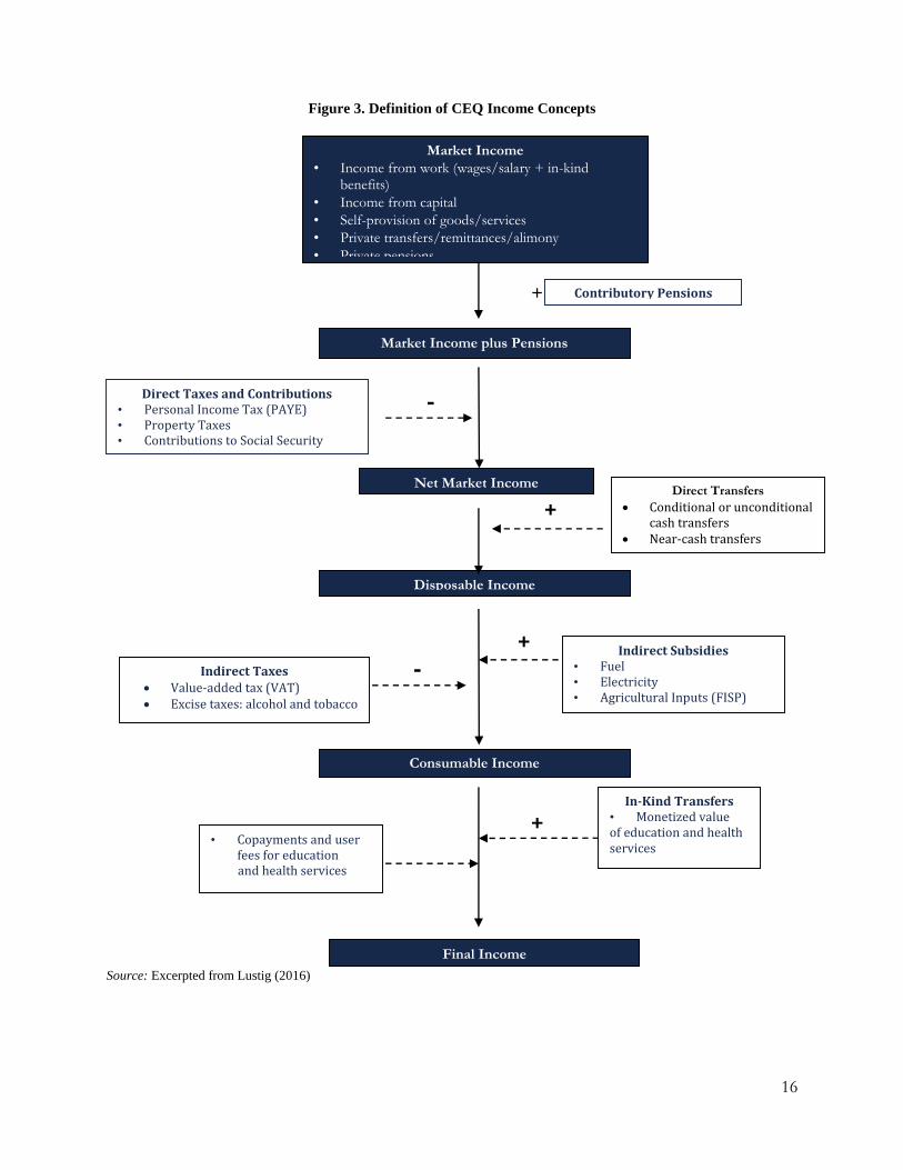
fiscal policy elements. Figure 5 summarizes the construction of these income concepts. Market Income, or

pre-fiscal income, is constructed by totaling for an individual all private sources of income: wages, capital

income, private transfer receipts, and gifts. The income concepts appearing in blue boxes below Market

Income include different elements of publicly provided transfers (or publicly mandated revenue

collections). Consequently, each is a post-fiscal income concept. Once the team has made the allocations,

it calculates measures of poverty and inequality.

Box 1: CEQ Terminology and Application in Zambia

Taxes and transfers, and fiscal policy more generally, are powerful instruments at the disposal of the state for reducing

extreme forms of material deprivation and narrowing the gap between economic elites and the rest. They can also help

to equalize opportunities, through public education for example, and thus increase social mobility and the productive

potential of the underprivileged. To assess whether governments are using these tools effectively, it is important to

be able to quantify how inequality and poverty change before and after the application of these fiscal policies.

To quantify the impact that fiscal policies have on income (or purchasing power, or welfare), the team first must

estimate a (counterfactual) income state that would be experienced before the transfers, benefits, and burdens

generated by the fiscal system are received or imposed. As a proxy for this state, the team defines pre-fiscal income

Ih as the cumulative income received from wages and salaries (that is, from labor market transactions) plus the market

value of auto-production and auto-consumption; from capital (including real estate); and from private transfers (such

as remittances from family members working abroad). The h subscript indexes a set of households (but equally could

index individuals).

The team then assembles a set of taxes and transfers Ti that it wants to examine: for example, Ti in Zambia might

include the Pay-as-You-Earn (PAYE) personal income tax and the Farmer Input Support Program (FISP). For each

household h, the team then uses the micro-data (for Zambia, the Living Conditions Monitoring Survey or LCMS), to

allocate shares (Sih) of each program i= 1,….I in Ti to each household h.

With the estimated shares, the team generates post-fiscal income at the household level Yh such that:

Yh = Ih - Σi Ti Sih. (1)

Figure 5 provides a schematic of the equation above. Figure 5 contains only one pre-fiscal income concept (Market

Income) and several post-fiscal income concepts (Disposable Income, Consumable Income, Final Income).

To determine the impact of the fiscal system on either poverty or inequality, the team takes the difference between its

preferred measures of poverty or inequality over the pre- and post-fiscal distributions. Naturally, the extent of the

fiscal system under consideration limits the team’s choice of the post-fiscal income concept. The impact of a fiscal

system that includes only two elements must be estimated over a post-fiscal income concept that includes only these

two elements.

To determine the impact of single tax or transfer (or a subset of taxes and transfers), the team takes the difference in

inequality (or poverty) at the post-fiscal income concept excluding the item in question (but including everything else

14

in the team’s fiscal system) and the post-fiscal income concept including the item in question (and also including

everything else in the team’s fiscal system).

A single tax or transfer (or a fiscal system) is inequality reducing when the addition of the fiscal item in question to

an income concept reduces measured inequality. A transfer is absolutely progressive if, when households are ranked

by pre-fiscal income levels, the cumulative household shares of the transfer are greater than cumulative population

shares. In a Lorenz curve figure, an absolutely progressive transfer’s concentration curve would lie above and to the

left of the 45 degree line. A transfer (tax) is relatively progressive if, when households are ranked by pre-fiscal income

levels, the cumulative household shares of the transfer (tax) are greater (less) than the cumulative household shares of

pre-fiscal income. In a Lorenz curve figure, a relatively progressive transfer’s (tax’s) concentration curve would lie

above and to the left (below and to the right) of the Lorenz curve for pre-fiscal income.

The team calls a transfer pro-poor when the transfers received, measured as a share or fraction of pre-transfer income,

decline with income. Notice that this definition of pro-poor includes cases in which the absolute transfer level declines

with income. For example, if a transfer is targeted to poor households, and non-poor households do not receive the

transfer, then, algebraically, transfers received are declining in income level. Because taxes always reduce purchasing

power, the team refrains from labeling taxes “pro-poor,” although when taxes paid (measured as a share of pre-tax

income) increase with income levels, they are by definition progressive. In everyday usage, for example, the team

often calls a marginal income tax rate schedule that has increasing marginal rates by taxable income bracket a

“progressive” income tax.

Two indicators we use to understand how a fiscal policy element is progressive or regressive are the concentration

shares and the incidence of a fiscal policy. Concentration shares calculate the share of the value of fiscal policy

captured by (or imposed on) a subset of the population such as the poorest 10 percent of individuals or the richest 10

percent of individuals. For example, if the richest 10 percent of Zambians pay 75 percent of the total PAYE taxes

collected in a given year, then the richest decile’s concentration share of PAYE taxes is 75 percent (and that in turn

implies that the other 90 percent of Zambians pay no more than 25 percent of total PAYE revenues). The incidence

of a fiscal policy element calculates the value of a benefit captured (or a tax imposed) relative to the value of income

before the benefit was received or before the tax was imposed.

While a pro-poor transfer is always progressive, the reverse is not necessarily true. Likewise, in a fiscal system with

more than one element, a pro-poor or progressive transfer (or a progressive tax) is not necessarily inequality reducing.

This study incorporates every type of fiscal policy element listed in Figure 3. The team adjudged the income

module in the LCMS to be unreliable.20 Team members felt the LCMS likely would lead to under-reporting of income

of those with little to no income from the (incomplete) LCMS list of income sources as well as of those with very high

incomes (from any source). Therefore, the study uses consumption expenditure as the measure of primary income.

The team assumes that total consumption expenditures––including the value of imputed rent for those living in owner-

occupied housing as well as the implied value of any auto-production/auto-consumption––are equal to the CEQ

Disposable Income concept (approximately in the middle of the flowchart in Figure 3). The team then works

“backwards” and “forwards” from Disposable Income to other CEQ income concepts to arrive at pre- and post-fiscal

measures.21

20 Consumption usually is preferred over income for four reasons. (1) Consumption is a better outcome indicator. Actual

consumption is related more closely to a person’s well-being in the sense of having enough to meet current basic needs. In contrast,

income is only one of the elements that will enable consumption of goods. Other elements include questions of access and

availability. (2) Consumption may reflect better a household’s ability to meet basic needs. Consumption expenditures reflect not

only the goods and services that a household can command based on its current income, but also whether that household can access

credit or insurance markets when current income is low or even negative. Thus, consumption can provide a better picture of actual

living standards than can current income, especially when incomes fluctuate greatly. (3) Consumption may be more accurately

measured than income. Especially in poor agrarian economies, incomes for rural households may fluctuate during the year, in line

with the harvest cycle. Fluctuation implies that householders may have difficulty in correctly recalling their incomes, causing the

income information to be of low quality. See, for example, Bollinger and Hirsch (2013) or Bollinger and Hirsch (2007) for thorough

treatments of the difficulties created by recall error and item non-response in socioeconomic survey income modules. (4) Large

shares of income are not monetized if households consume their own production or trade it for other goods. 21 Consumption expenditure is the team’s primary income measure. Moreover, all other income concepts including market income

are derived from consumption expenditure. For these reasons, the team does not create a Taxable Income (TI) concept. Other CEQ

15

Assessments do produce this income concept when relevant. Creating a Taxable Income concept requires knowledge of the

composition of Market Income. A Zambian household’s expenditure profile in the LCMS cannot provide any information on the

composition of its income. For the same reason, the team is unable to say anything about the savings or current asset profiles of

LCMS households: a current consumption expenditure profile provides no information on either investment spending or on the

returns accruing to any household assets.

16

Figure 3. Definition of CEQ Income Concepts

Source: Excerpted from Lustig (2016)

Market Income

• Income from work (wages/salary + in-kind benefits)

• Income from capital

• Self-provision of goods/services

• Private transfers/remittances/alimony

• Private pensions

Contributory Pensions

Direct Taxes and Contributions • Personal Income Tax (PAYE) • Property Taxes • Contributions to Social Security

Net Market Income

Market Income plus Pensions

+

Disposable Income

Direct Transfers

Conditional or unconditional cash transfers

Near-cash transfers

+

Indirect Subsidies • Fuel • Electricity • Agricultural Inputs (FISP)

• Agricultural inputs

+

Indirect Taxes Value-added tax (VAT) Excise taxes: alcohol and tobacco

-

In-Kind Transfers • Monetized value of education and health services

+ • Copayments and user

fees for education and health services

-

Consumable Income

Final Income

-

17

Zambia’s pre-fiscal income measure includes income received from the public pension system. Market

income reflects income before any transfers (including public spending on health and education, farming

inputs, fuel and energy subsidies, and unconditional cash transfers) or taxes (including personal income

taxes, VAT, and alcohol and tobacco excises) have been added. However, two scenarios for treating

contributory pensions usually are elaborated in the standard CEQ fiscal incidence methodology. These two

scenarios are (1) contributory pensions as deferred income (and pension contributions as voluntary saving)

or (2) contributory pensions as a government transfer (and pension contributions as a tax on income).

Zambia’s contributory pension system is available only to civil servants while employee contributions make

up an insignificant portion of government and pension-system revenues. In other words, in Zambia, the

contributory pension system functions much as a non-wage salary payment (to civil servants). Therefore,

the team’s pre-fiscal income measure becomes Market Income + Pensions (second blue box from top in

Figure 9).

Data Sources

The primary dataset providing the individual- and household-level information necessary to allocate

fiscal policy elements22 is the 2015 Zambia Living Conditions Monitoring Survey. This study focuses

solely on fiscal year 2015 because that is the last year for which LCMS is available. LCMS (2015) includes

modules covering health, education, economic and labor market activity, household consumption

expenditure, agricultural production, and rent (or, for owner-occupied housing, imputed rent). LCMS also

provides a roster per household that provides individual, demographic, and dwelling characteristics. The

2015 LCMS uses the 2010 Census of Population and Housing as the sampling frame and is representative

at the national level, by urban and rural areas, and by province. The survey was administered to

approximately 12,250 households, who comprised almost 63,000 individuals.

The team uses the 2013–14 Zambia Demographic and Health Survey (DHS) to impute a propensity

to visit public healthcare providers as well as to calculate shares of all recorded visits by household

type. The LCMS 2015 healthcare utilization module asks household members to recall whether they had

an illness or medical condition over the past two weeks for which they sought attention at a healthcare

facility. The Zambia 2013–2014 DHS includes more complete information on healthcare use––over a 12

month recall period, and not conditional upon illness or injury ––in a nationally representative sample

survey of women and men of reproductive age. The team uses propensity scores and shares of total clinic

and hospital-level visits estimated within the DHS to generate a household expected public healthcare

benefit received within the LCMS 2015.23

The source for total revenues collected by the government from households––via the personal income

tax, VAT, and excise taxes––is the 2015 Annual Economic Report published by the Ministry of

Finance. To impute “effective” or actual, prevailing rates (which may differ from statutory rates), the team

first scales down the expected tax take from LCMS households. Scaling is done so that the ratio of tax

revenues in final or audited budget reports to Private Final Household Consumption Expenditure in Zambia

National Accounts data are equivalent to the ratio of VAT collections from LCMS households to the value

of cumulative LCMS household consumption expenditure.

22 The allocations––including the assumptions and choices implicit in them––are described in the following section. 23 The DHS-to-LCMS imputation is made by estimating propensity scores (describing the likelihood of choosing a public healthcare

provider when healthcare services are acquired) in the DHS based on individual and household characteristics (education,

household size, and region) and income rank and then creating fitted values of that propensity score in the LCMS using the

analogous LCMS characteristics. We also use the DHS to estimate a decile’s share of all clinic-level healthcare visits and all

hospital-level healthcare visits over a 12-month period; in that estimation DHS households are ranked according to a household

wealth variable recorded in the DHS itself. We then assume that the share of total visits for a DHS decile are equivalent to an

LCMS decile’s share of total visits.

18

The team also took from the 2015 Annual Economic Report the government’s expenditures on

electricity, fuel subsidies, the Farmer Input Support Program (FISP), and in-kind healthcare and

education transfers. The team scaled these subsidies and in-kind transfers to equal the scaling of taxes.

The Social Cash Transfer (SCT) program’s 2015 expenditures as well as the SCT 2015 beneficiary total

were provided by the Ministry of Community Development and Social Welfare. The team found that total

SCT expenditures allocated among LCMS households were approximately equal to confirmed

expenditures, and the average transfer per household is approximately equal to the number of confirmed

SCT expenditures divided by the number of confirmed SCT recipients. Thus, the total amount of direct

transfer expenditures allocated is not scaled in the way that the other fiscal policy elements described above

are.

Allocation Overview

When and where possible, the study allocates fiscal policy elements to individuals or households based on

direct observation. For example, when an individual queried in a socioeconomic survey is asked to recall

how much she has paid in VAT on all her purchases in the last seven days, or is asked to provide receipts

detailing VAT payments, the team directly “observes” the total VAT collection from her. These VAT

payments recorded by individuals then are assumed to be the same VAT revenues listed in the executive,

administrative, and other budget reporting for the same year.

In Zambia’s LCMS, however, very few fiscal policy elements could be allocated via direct

observation.24 Instead, the study uses imputation and simulation (sometimes in combination with

direct observation). Imputation is used when a survey unit’s benefit recipient (taxpayer) status must be

inferred (rather than directly identified), or the amount received (paid) is retrieved from administrative

records or program (tax) rules (rather than directly recorded in the survey); or both. Simulation is available

when neither direct identification nor imputation can be used, so that the beneficiaries (taxpayers) and the

amount received (paid) are simulated based on the program (tax).25 The subheadings below provide a

summary of allocation assumptions and decisions for various fiscal policy element in this study.

Personal Income Taxes

Direct (personal income tax) taxpayer status is imputed based on a simple sum of “0/1” indicators

that describe the level of formality in an individual’s participation in the labor market, whether the

same individual makes social security contributions, and whether the individual makes pension

contributions. For LCMS households with at least one individual imputed to be a taxpayer, the household

tax burden is simulated according to the statutory marginal personal income tax rate schedule. The

individual’s total personal income tax burden is scaled down. The goal is that the total personal income

taxes collected from LCMS households relative to the total value of consumption expenditure in the LCMS,

are found to be equivalent to the total personal income tax collections in budget documents relative to the

value of total final household consumption expenditure in the national accounts.

Among the set of likely taxpayers in the LCMS, we replicated the distribution of the concentration shares

of PAYE taxes paid according to administrative records from the Zambian Revenue Authority (ZRA). That

is, we had actual, anonymous taxpayer records from the ZRA which allowed us to calculate the rank

position of all taxpayers (according to their total taxes paid) and their concentration shares of taxes paid.

24 Access to publicly delivered health and education services is observed directly as is the purchase of subsidized fuels and

electricity. However, the subsidy received for transactions in these services and goods must be imputed or simulated. 25 Imputation using secondary sources is used to improve the validity of an imputation of beneficiary or taxpayer status in the

LCMS by taking confirmed demographic or regional (or other) characteristics of beneficiaries (taxpayers) from a secondary source

and replicating the distribution of those characteristics in the imputed beneficiary LCMS population. For a detailed description of

these and other allocation methods, see Higgins and Lustig 2017.

19

We then re-created that distribution within our set of likely LCMS taxpayers, so that, for example, the top

10 percent of likely LCMS taxpayers (ranked by income) paid the same share – 37.6 percent – of total

PAYE taxes collected from all LCMS households that the top 10 percent of actual taxpayers paid in

confirmed PAYE collections from all Zambian households. Likewise, the bottom 10 percent of likely

LCMS taxpayers paid the same 0.9 percent share of total PAYE taxes collected from all LCMS households

that the bottom 10 percent taxpayers paid in confirmed PAYE collections form all Zambian households.

Recreating the confirmed distribution of concentration shares of actual taxpayers in the LCMS increased

PAYE’s overall progressivity.

Direct Transfers

The LCMS does not directly identify SCT beneficiary households. Instead, the team simulates SCT

eligibility based on household characteristics that inform the actual SCT targeting and selection. The study

takes as eligible households those living in regions in which SCT is available and who have 1 (or more)

disabled individuals; or have a dependency ratio of 3 or greater; or have a female household head. The team

then mixes a poverty-targeted allocation rule with a randomized allocation rule (among eligible households)

in each SCT region represented in the LCMS. This “mixed” poverty-targeted (among SCT-eligible) and

random allocation (among SCT-eligible) results in a “leakage” rate of approximately 25 percent overall: 25

percent of the available SCT benefits are received by non-poor households.

The number of SCT beneficiaries in 2015 is 166,269. SCT benefit amounts transferred––140 Zambian

Kwacha per month for households with at least 1 disabled member and 70 Kwacha per month for other

households––are simulated according to program rules. Finally, the regional SCT beneficiary quotas are

replicated within the LCMS so that the number of SCT beneficiaries (and benefits) allocated within the

LCMS matches (by region) the actual SCT beneficiaries (and benefits).

Farmer Input Support Program (FISP) Subsidies

FISP delivers subsidized agricultural inputs through authorized resellers (farmer cooperatives). The

Agricultural Enterprise Expenses module in the LCMS asks those whose livelihood is in agriculture where

they buy inputs. To qualify for FISP support, farmers must belong to a cooperative or farmer association

and have the capacity to grow one ha of maize.

LCMS households involved in agricultural production who buy fertilizer at farmer cooperatives are imputed

to be FISP recipients. According to the team’s estimations based on the LCMS 2015, approximately

410,000 households received FISP (proxied as those who receive inorganic fertilizer through cooperatives)

in the growing season that spanned 2014–2015. This number is close to official government figures. The

subsidy value of a FISP purchase is assumed to be a flat 1,800 Kwacha (regardless of the amount spent on

fertilizers purchased at cooperatives. This rate is taken from information provided by World Bank

Agriculture team colleagues XXXX. Thus, total FISP expenditures allocated to LCMS households are

equivalent to 1,800 times the total number of households who indicate making fertilizer purchases through

cooperatives.

Energy subsidies and indirect taxes

Fuel and electricity subsidies, VAT, and alcohol and tobacco excises are imputed based on household

consumption expenditure records. In other words, when households record purchases of energy, goods

that are standard-rated under the 2015 VAT schedule, or alcohol or tobacco, the subsidy or indirect tax

payment implicit in this purchase is imputed based on the relevant subsidy or tax schedule. For example, if

20

an LCMS household records $110 in alcohol purchases over a month, and the excise rate on alcohol

purchases is 10 percent, the household is imputed to have purchased $100 of alcohol and paid $10 in excises.

The team captures the estimated impacts of energy subsidies and indirect tax policies as they are

actually implemented, not as they are described statutorily. For example, not all energy is consumed

by households, and not all goods and services are standard-rated VAT products. In Zambia, the mining

sector accounts for a large portion of total electricity subsidy expenditure. Households’ electricity purchases

account for a much smaller share. The subsidies captured by the mining sector likely are passed on as lower

mining-sector output prices to other firms or producers that use mining products as inputs. When these

firms pass on embedded input subsidies to the final prices of their own goods, even subsides captured by

the mining sector can produce a benefit for the final consumer. This study estimates these indirect effects

of subsidies and the VAT regime and includes the indirect benefit (or burden) via the same imputation

procedure based on consumption expenditure records described above.26

In-kind transfers

Receipt of in-kind benefits is based on directly identified utilization of the public education or public

healthcare system. The LCMS records how many household members are enrolled in the public education

system (and at what levels) and whether any household members recently visited a public healthcare

facility. The monetized value of the in-kind transfer is based on the “government cost” approach. For

example, total education expenditures are divided by the total number of users (students) to get a uniform

per-user cost of producing and delivering the service. This per-user cost then is defined as the value of the

transfer received. This cost represents what the utilizing household would have to pay to acquire the service

at the government’s cost.

We used disaggregated (by facility type) administrative data to guide our estimation of the government cost

of a healthcare or education service acquired. For health, we used administrative summaries of Health

Ministry and Ministry of Community Development and Mother and Child Health expenditure to allocate

specific expenditures to hospital and clinical care providers. For example, the public expenditures

transferred to public hospitals for personnel and medical goods (including medicines) is not equivalent

overall or on a per-facility basis to public expenditures for the same items for public clinic-based healthcare.

Also for health, we utilized Zambia’s DHS to impute to each LCMS household a propensity to visit a public

healthcare provider (when healthcare services were acquired) as well as an expected share of total clinic-

level and hospital-level visits over a 12 month period. Each LCMS household then has an imputed share

of clinic-level and hospital-level public healthcare expenditures that may be different from their actual share

of clinic-level and hospital-level healthcare expenditures over the 2-week recall period and conditional

upon illness or injury recorded in the LCMS. We use the imputed share over a 12-month period to allocate

public healthcare expenditures.27

Note that for both public health and education services, the estimate of the value of the benefit we allocate

is limited by the information available. For example, we can separate clinic-level visits from hospital visits

in the micro-data; and we can separate clinic-level public expenditures from hospital-level expenditures;

26 This study follows the methodology developed described in the Commitment to Equity Handbook (Lustig, 2016), Chapter 4 to

allocate the indirect impact of indirect taxes on the prices of goods and services acquired in the private market. Basically, the

Handbook suggests solving a price-shifting model – with an Input-Output matrix as the empirical description of price determination

in the production side of the economy – assuming inelastic demand for all goods and services and fixed technologies of production.

That is, producers “push” any input taxes paid (subsidies received) onto the final price of the goods and services thereby raising

prices (lowering prices) relative to a no tax (no subsidy) counterfactual. 27 Additional details about each of these allocation procedures, including the assumptions made, is available in section C of the

Zambia CEQ Master Workbook.

21

but we cannot further determine exactly which service was received at either clinic or hospital. As we are

unable to describe the variation in the value of the services provided at any level, we cannot estimate the

distributional impact of higher expenditures for more complicated procedures (for example) at any level.

A “public healthcare service – clinic level” benefit can be considered an average value across all services

provided at the clinic level.

RESULTS

Redistributive Effects of Zambia’s Fiscal System

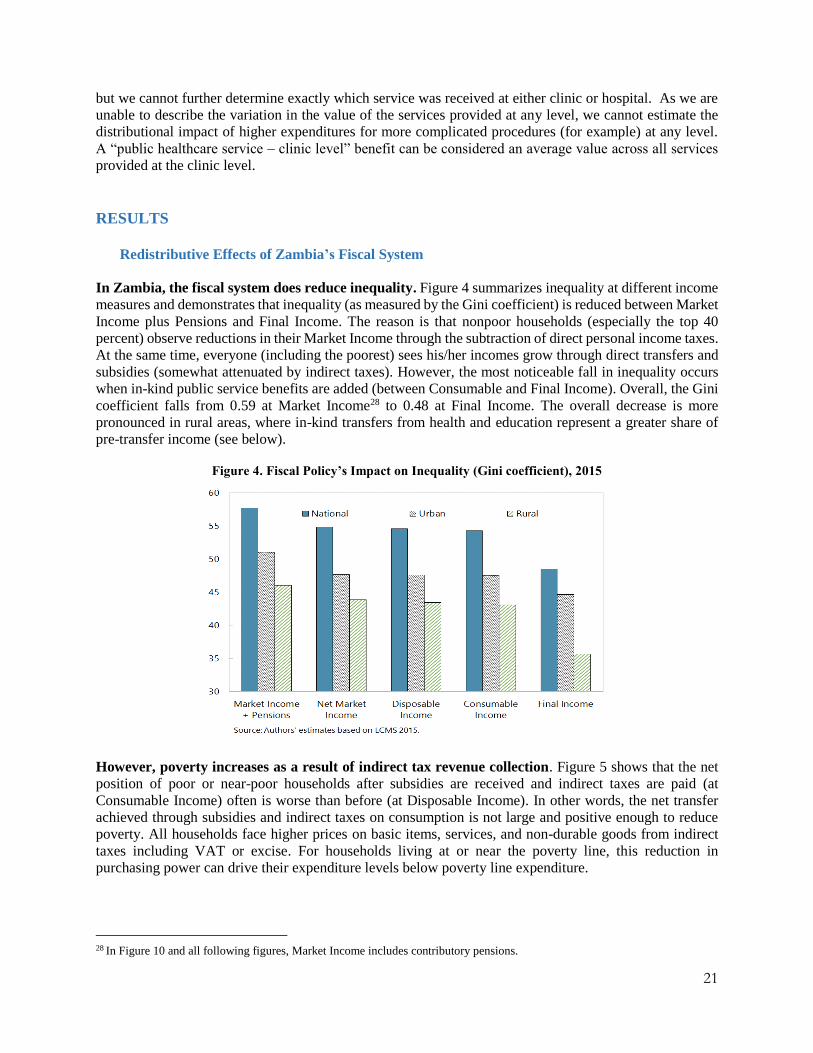
In Zambia, the fiscal system does reduce inequality. Figure 4 summarizes inequality at different income

measures and demonstrates that inequality (as measured by the Gini coefficient) is reduced between Market

Income plus Pensions and Final Income. The reason is that nonpoor households (especially the top 40

percent) observe reductions in their Market Income through the subtraction of direct personal income taxes.

At the same time, everyone (including the poorest) sees his/her incomes grow through direct transfers and

subsidies (somewhat attenuated by indirect taxes). However, the most noticeable fall in inequality occurs

when in-kind public service benefits are added (between Consumable and Final Income). Overall, the Gini

coefficient falls from 0.59 at Market Income28 to 0.48 at Final Income. The overall decrease is more

pronounced in rural areas, where in-kind transfers from health and education represent a greater share of

pre-transfer income (see below).

Figure 4. Fiscal Policy’s Impact on Inequality (Gini coefficient), 2015

However, poverty increases as a result of indirect tax revenue collection. Figure 5 shows that the net

position of poor or near-poor households after subsidies are received and indirect taxes are paid (at

Consumable Income) often is worse than before (at Disposable Income). In other words, the net transfer

achieved through subsidies and indirect taxes on consumption is not large and positive enough to reduce

poverty. All households face higher prices on basic items, services, and non-durable goods from indirect

taxes including VAT or excise. For households living at or near the poverty line, this reduction in

purchasing power can drive their expenditure levels below poverty line expenditure.

28 In Figure 10 and all following figures, Market Income includes contributory pensions.

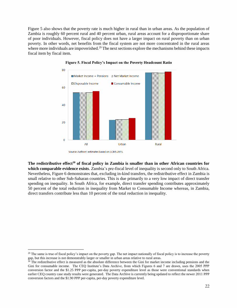
22

Figure 5 also shows that the poverty rate is much higher in rural than in urban areas. As the population of

Zambia is roughly 60 percent rural and 40 percent urban, rural areas account for a disproportionate share

of poor individuals. However, fiscal policy does not have a larger impact on rural poverty than on urban

poverty. In other words, net benefits from the fiscal system are not more concentrated in the rural areas

where more individuals are impoverished.29 The next sections explore the mechanisms behind these impacts

fiscal item by fiscal item.

Figure 5. Fiscal Policy’s Impact on the Poverty Headcount Ratio

The redistributive effect30 of fiscal policy in Zambia is smaller than in other African countries for

which comparable evidence exists. Zambia’s pre-fiscal level of inequality is second only to South Africa.

Nevertheless, Figure 6 demonstrates that, excluding in-kind transfers, the redistributive effect in Zambia is

small relative to other Sub-Saharan countries. This is due primarily to a very low impact of direct transfer

spending on inequality. In South Africa, for example, direct transfer spending contributes approximately

50 percent of the total reduction in inequality from Market to Consumable Income whereas, in Zambia,

direct transfers contribute less than 10 percent of the total reduction in inequality.

29 The same is true of fiscal policy’s impact on the poverty gap. The net impact nationally of fiscal policy is to increase the poverty

gap, but this increase is not demonstrably larger or smaller in urban areas relative to rural areas. 30 The redistributive effect is measured as the absolute difference between the Gini for market income including pensions and the

Gini for consumable income. The CEQ Institute’s Data Archive, from which Figures 6 and 7 are drawn, uses the 2005 PPP

conversion factor and the $1.25 PPP per-capita, per-day poverty expenditure level as those were conventional standards when

earlier CEQ country case study results were generated. The Data Archive is currently being updated to reflect the newer 2011 PPP

conversion factors and the $1.90 PPP per-capita, per-day poverty expenditure level.

23

Figure 6. Fiscal Policy’s Impact on Inequality (bars);

Initial Inequality (dots), select countries/years

Figure 7. Fiscal Policy’s Impact On Poverty

Headcount Ratio (bars); Pre-fiscal Poverty

Headcount Rate (dots), $1.25 PPP (2005) poverty

line, select countries/years (%)

The contribution of fiscal policy to increasing poverty is shared by other countries in Africa. Figure

7 shows that in most low-income countries in Africa including Zambia, fiscal policy (excluding in-kind

transfers) contributes to an increase in the poverty headcount ratio. In Tanzania, for example, the fiscal

system relies heavily on indirect taxes. Sixty-seven percent of all revenue from taxes comes from indirect

taxes alone. Moreover, the value-added tax and excise duties together are larger (as a source of revenues)

than revenues collected through the personal income tax system. Although the Tanzanian excise covers

socially costly goods including refined petroleum (for automobiles and heavy machinery), tobacco, and

alcohol, it also covers near-necessities such as bottled water, mobile phone air time, and kerosene (used as

cooking gas).

Zambia’s fiscal system is similarly weighted toward indirect taxes. Although the number of goods covered

by the Zambian excise system is fewer than in Tanzania, the VAT share of indirect taxes is larger in Zambia

than in Tanzania. Consequently, nearly every person–rich or poor––is affected by the Zambian indirect tax

system because at least one of the items she consumes regularly carries an explicit or implicit indirect tax

charge. As a result, after direct transfers and subsidies are received and direct and indirect taxes are paid,

most Zambian households’ net purchasing power is reduced.

How Many Zambians Are Impoverished or Made Better off by Fiscal Policy?

Calculating the poverty headcount before and after fiscal policy elements are applied gives a broad

indication of the advantage or disadvantage created by this policy. If the poverty headcount is higher

after the policy has been applied, the policy has disadvantaged some individuals. However, any individual

receiving (as benefits) a fiscal expenditure sees his/her income increase; and any person paying a tax (or

other revenue collection) sees her/his income decrease. The team can summarize these individual gains and

losses through the Fiscal Impoverishment (FI) and Fiscal Gains to the Poor (FGP) indices (first proposed

by Higgins and Lustig 2016).

The Fiscal Impoverishment (FI) Index “tracks” the pre-fiscal income of households who become poor

(or start poor and are made poorer) following the execution of a fiscal policy (or a set of fiscal

policies). The FI index can determine how much these households’ incomes had decreased and,

consequently, by how much they were impoverished. Table 3 shows that, if poverty is measured using the

$1.25 PPP [2005] line, after the addition of the personal income tax, the SCT transfer, the indirect VAT

and excise taxes; as well as the FISP, electricity, and fuel subsidies to Market Income, the net position of

24

all Zambian households is such that just over 50 percent of the population experienced one of the following

two outcomes. For some of these households, (1) pre-fiscal incomes were below the poverty line and net

contributions to the fiscal system were larger than net receipts and so total purchasing power was reduced

even further. For others, (2) pre-fiscal incomes were above the poverty line, net contributions to the fiscal

system were larger than net receipts, and total purchasing power was reduced such that post-fiscal incomes

(through Consumable Income) were below the poverty line.

Fiscal policy in Zambia impoverishes more people than do the fiscal policies of lower middle and

middle-income countries in Africa, Asia, and Latin America. Table 4 indicates that Zambia’s FI index

puts it at the bottom end of the distribution of FI performance: only Tanzania generates impoverishment

(via fiscal policy) at a rate comparable to Zambia. Column 5, which presents FI among the individuals who

are poor (rather than in the population at large), shows that even in Sri Lanka, where FI is negligible when

measured as a percent of the total population, approximately one-third of the consumable-income poor have

been impoverished by the (net) fiscal system. In Tanzania, Zambia, and Ethiopia, however, approximately

85 to 100 percent of the population measured as post-fiscal poor were impoverished by the fiscal system.

Table 3. Fiscal Impoverishment, ca. 2010

Country, survey year

(1) Market

income plus contributory

pensions poverty

headcount (%)

(2) Change in poverty

headcount (percentage

points)

(3) Market

income plus contributory

pensions inequality

(Gini)

(4) Fiscally

impoverished as % of

population

(5) Fiscally

impoverished as % of

consumable income poor

Armenia, 2011 12.8 -1.0 40.3 6.2 52.3 Bolivia, 2009 10.0 -0.2 50.3 6.6 63.2 Dominican Republic, 2013 5.7 -0.8 51.4 1.0 16.3 Ethiopia, 2011 31.9 1.3 32.2 28.5 83.2 Ghana, 2013 6.0 0.8 43.7 5.1 76.6 Guatemala, 2010 5.6 0.1 51.3 7.0 62.2 Indonesia, 2012 12.1 -1.5 39.4 4.1 39.2 Sri Lanka, 2010 5.0 -0.7 37.1 1.6 36.4 Tanzania, 2011 43.7 7.8 38.2 50.9 98.6 Uganda, 2012/13 17.9 0.1 41.3 12.2 67.7 Zambia, 2015 36.0 2.8 55.0 52.6 84.3

Sources: Zambia: authors’ calculations based on LMCS 2015; Uganda: Haas and others (2016); all others: Higgins and Lustig

(2016).

The FGP index is the mirror of FI. The FGP index tracks pre-fiscal poor households receiving (net)

benefits to determine much their incomes are increased from this receipt. The pre-fiscal poor are those

whose market incomes (including pensions) are below the poverty line. At Consumable Income, and using

the same $1.25 PPP [2005] poverty line as in table 3, 16 percent of the pre-fiscal poor receive (net) positive

transfers from Zambian fiscal policy. The fiscal system adds an average of approximately 21 percent to the

pre-fiscal-income of the poor individuals who receive positive net transfers.

Overall, the fiscal system adds less income to fewer of the pre-fisc poor and takes away more income from

more of the post-fisc poor. By now, the result is familiar: on net, the poverty headcount increases between

Market Income plus Pensions and Consumable Income.

Education Expenditures Are the Main Fiscal Instrument for Reducing Inequality

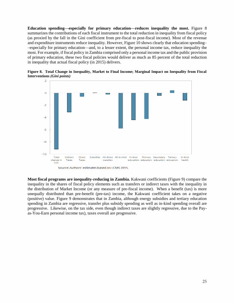
25

Education spending––especially for primary education––reduces inequality the most. Figure 8

summarizes the contributions of each fiscal instrument to the total reduction in inequality from fiscal policy

(as proxied by the fall in the Gini coefficient from pre-fiscal to post-fiscal income). Most of the revenue

and expenditure instruments reduce inequality. However, Figure 10 shows clearly that education spending–

–especially for primary education––and, to a lesser extent, the personal income tax, reduce inequality the

most. For example, if fiscal policy in Zambia comprised only a personal income tax and the public provision

of primary education, these two fiscal policies would deliver as much as 85 percent of the total reduction

in inequality that actual fiscal policy (in 2015) delivers.

Figure 8. Total Change in Inequality, Market to Final Income; Marginal Impact on Inequality from Fiscal

Interventions (Gini points)

Most fiscal programs are inequality-reducing in Zambia. Kakwani coefficients (Figure 9) compare the

inequality in the shares of fiscal policy elements such as transfers or indirect taxes with the inequality in

the distribution of Market Income (or any measure of pre-fiscal income). When a benefit (tax) is more

unequally distributed than pre-benefit (pre-tax) income, the Kakwani coefficient takes on a negative

(positive) value. Figure 9 demonstrates that in Zambia, although energy subsidies and tertiary education

spending in Zambia are regressive, transfer plus subsidy spending as well as in-kind spending overall are

progressive. Likewise, on the tax side, even though indirect taxes are slightly regressive, due to the Pay-

as-You-Earn personal income tax), taxes overall are progressive.

26

Figure 9. Kakwani Coefficients for Fiscal Policy Elements in Zambia, 2015

Over a two-week period, poor households utilize public healthcare services more often. Figure 10

indicates that individuals from poorer households are more likely to face adverse health events (over a two-

week period) than those from richer households. In addition, conditional on an adverse health event,

individuals from poorer households are more likely to use the public healthcare clinic system, and at least

as likely to use the public hospital system, than individuals from richer households.

Over an entire year poor households capture smaller shares of the in-kind public health benefits

available, however. Figure 11 shows the concentration shares for health, or the share of total in-kind

public health benefits captured, for each market income decile, when we use the Zambia DHS to estimate

public healthcare service utilization over an entire year and not conditional upon illness or injury. The

height of the bars represent the total concentration share, and the orange- and blue-shaded sub-bars represent

the contribution of hospital- and clinic-level care, respectively, to the overall concentration share. As the

LCMS also indicates, richer households utilize clinic-level public healthcare less often than richer

households in the DHS. However, richer households in the DHS utilize hospital-level public healthcare

(over a year-long period) much more frequently than poor households.

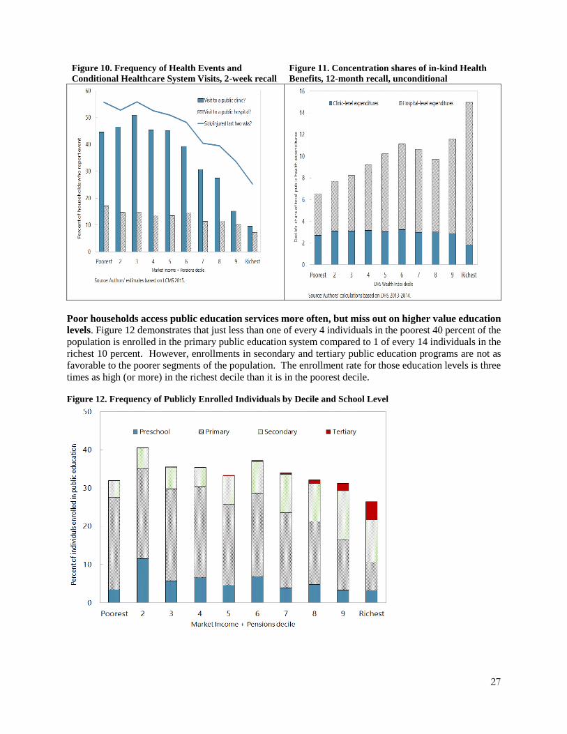
27

Figure 10. Frequency of Health Events and

Conditional Healthcare System Visits, 2-week recall Figure 11. Concentration shares of in-kind Health

Benefits, 12-month recall, unconditional

Poor households access public education services more often, but miss out on higher value education

levels. Figure 12 demonstrates that just less than one of every 4 individuals in the poorest 40 percent of the

population is enrolled in the primary public education system compared to 1 of every 14 individuals in the

richest 10 percent. However, enrollments in secondary and tertiary public education programs are not as

favorable to the poorer segments of the population. The enrollment rate for those education levels is three

times as high (or more) in the richest decile than it is in the poorest decile.

Figure 12. Frequency of Publicly Enrolled Individuals by Decile and School Level

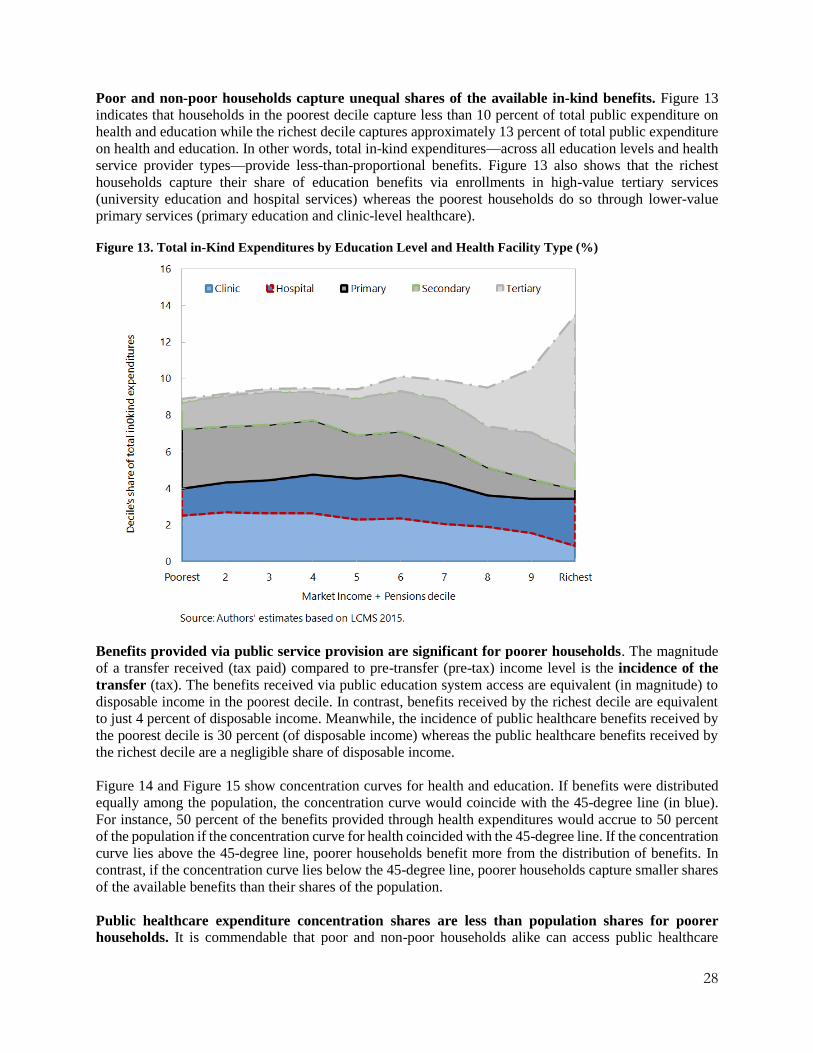
28

Poor and non-poor households capture unequal shares of the available in-kind benefits. Figure 13

indicates that households in the poorest decile capture less than 10 percent of total public expenditure on

health and education while the richest decile captures approximately 13 percent of total public expenditure

on health and education. In other words, total in-kind expenditures––across all education levels and health

service provider types––provide less-than-proportional benefits. Figure 13 also shows that the richest

households capture their share of education benefits via enrollments in high-value tertiary services

(university education and hospital services) whereas the poorest households do so through lower-value

primary services (primary education and clinic-level healthcare).

Figure 13. Total in-Kind Expenditures by Education Level and Health Facility Type (%)

Benefits provided via public service provision are significant for poorer households. The magnitude

of a transfer received (tax paid) compared to pre-transfer (pre-tax) income level is the incidence of the

transfer (tax). The benefits received via public education system access are equivalent (in magnitude) to

disposable income in the poorest decile. In contrast, benefits received by the richest decile are equivalent

to just 4 percent of disposable income. Meanwhile, the incidence of public healthcare benefits received by

the poorest decile is 30 percent (of disposable income) whereas the public healthcare benefits received by

the richest decile are a negligible share of disposable income.

Figure 14 and Figure 15 show concentration curves for health and education. If benefits were distributed

equally among the population, the concentration curve would coincide with the 45-degree line (in blue).

For instance, 50 percent of the benefits provided through health expenditures would accrue to 50 percent

of the population if the concentration curve for health coincided with the 45-degree line. If the concentration

curve lies above the 45-degree line, poorer households benefit more from the distribution of benefits. In

contrast, if the concentration curve lies below the 45-degree line, poorer households capture smaller shares

of the available benefits than their shares of the population.

Public healthcare expenditure concentration shares are less than population shares for poorer

households. It is commendable that poor and non-poor households alike can access public healthcare

29

services, and that poor households manage conditional access to the public healthcare system at the clinic

level as or more frequently than do non-poor households. However, per-capita benefits overall are greater

in richer households because of a higher likelihood of a higher-valued hospital visits among individuals in

non-poor households (Figure 14).

Figure 14. Health Benefits: Cumulative

Concentration Shares

Figure 15. Education Benefits: Cumulative

Concentration Shares

Source: Authors’ calculations based on LCMS 2015.

Public education expenditure is pro-poor only at the primary levels. The distributional pattern is very

pro-rich for early childhood education/pre-school, secondary school, and especially for colleges and

universities (Figure 15). Households in the poorest 50 percent of the population receive almost none of the

public tertiary education benefits available because these households contribute very few of the students

enrolled in public tertiary education. Public education expenditures might look more regressively

distributed if poorer households contributed primary school students at the same lower rate as do non-poor

households.

Cash Transfers Have Limited Coverage and Are Small

The Social Cash Transfer Scheme (SCTS) is progressive but provides low coverage. Figure 16 shows

that the bottom 40 percent of the population (ranked by Market Income + Pensions) receives nearly 70

percent of the SCTS benefits available. However, given the program’s coverage, even assuming perfect

targeting, the SCT would cover no more than 20 percent of the extreme poor (in 2015). Even under the

unlikely hypothesis that families could only receive one type of benefit from the multiple existing social

programs in Zambia and that these benefits are perfectly targeted to the extreme poor, all of the major

programs combined would cover less than 50 percent of the extreme poor.

Furthermore, the SCTS provides low benefits relative to needs. Despite the multiple positive impacts

of the transfer scheme,31 with ZMW 70 per month (US$10), a beneficiary family can cover approximately

10 percent of the cost of a monthly food basket that provides the minimum energy requirements for a family

of 6.32 Far from supplying a nutritionally balanced diet, this amount will buy only a 25-kg bag of white

maize and 1 liter of cooking oil per month per family. Over 300,000 children of secondary school age are

31 The SCT’s randomized control trial reveals multiple positive impacts at 2- and 3-year intervals. The grant helped reduce poverty

in beneficiary households and increased their consumption. The children in the beneficiary households experienced measurable

benefits, such as reduced incidence of diarrhea and lower school drop-out rates at the transitional ages of 11 to 14. The evaluation

also found a multiplier effect of 50%–70% attributable primarily to productive activities. 32 The cost of the food basket for a family of 6 for 1 month is estimated to cost KWA 686 at average annual prices of April/May

2015 (CSO and World Bank 2016).

30

members of these families. For most of these children, the SCTS benefit would be the only source of cash

income to cover school fees, which could cost between ZMW 2000–4000. Hence, very few families can

aspire to cover any portion of the school cost.

The SCT benefit package is too small to change the poverty headcount ratio. Additionally, SCT

coverage levels are not high enough to reduce the poverty gap. For example, the reduction in the poverty

gap from the SCT transfer is approximately 1 percent. When the SCT transfer is added to incomes, the

squared poverty gap––sometimes called an index of the severity of poverty––drops by approximately 2

points.

Figure 16. SCT Eligible Beneficiaries and SCT Coverage, 2015

Vast Majority of Subsidies Accrue to Non-Poor Households

The 2015 LCMS found that approximately 31 percent of households nationally are connected to the energy

grid. For urban households only, coverage rises to almost 70 percent, but only 4.4 percent of rural

households are connected. This infrastructure pattern limits the depth and breadth of energy subsidy

coverage. For example, less than 2 percent of households in the poorest 50 percent of the population can

benefit directly from the electricity subsidy while less than 1 percent of households in the poorest 50 percent

benefit directly from the fuel subsidy (Figure 17).

Figure 17. Electricity, Fuel, and FISP Subsidy Coverage Rates, 2015

31

FISP benefits primarily middle-income farmers. According to the LCMS 2015, approximately 410,000

households received FISP (proxied as those who receive inorganic fertilizer through cooperatives) during

the growing season spanning 2014 and 2015.33 FISP coverage rates are highest for farmers in the middle of

the income distribution (figure 17). As FISP delivers a uniform benefit amount to all beneficiaries (see

above), the bottom 60 percent of households capture over 75 percent of the FISP benefits while the richest

20 percent of households capture 7 percent of FISP benefits.

Program rules and corruption likely are preventing FISP from achieving pro-poor targeting. Diversion in

FISP, measured as the difference between what was allocated for FISP expenditure on inputs and what was

actually received by the targeted population, is estimated to be approximately 38 percent in Zambia (Mason

and Jayne 2013). Program rules may also prevent FISP benefits from being received by the poorest

agricultural households. To qualify for FISP support, farmers must belong to a cooperative or farmer

association and have the capacity to grow one hectare of maize. The result is that land-constrained (mostly

poor) households cannot access the funds from the program.

Fuel and electricity subsidies are regressive: subsidy incidence rises with income. The richest 10

percent of households capture nearly 90 percent of the total fuel available subsidies and over 50 percent of

the total available electricity subsidies (figures 18 and figure 19). Most rural households consume little fuel

or electricity directly, but benefit indirectly through, for example, lower prices for transport (because fuel

is a major input in transport). More benefits from fuel subsidies are concentrated in the richest urban deciles

than in the richest rural deciles. The benefits from electricity subsidies are captured in similar proportions

by the richest households in urban and rural areas.

Figure 18. Fuel Subsidy Concentration (%) Figure 19. Electricity Subsidy Concentration (%)

Energy subsides also have indirect welfare impacts by depressing prices for other non-fuel goods.

These indirect impacts34 are more equitably distributed than the subsidies themselves, but, relative to

33 This number is close to official government figures. 34 The indirect impacts of a subsidy regime are delivered via the production side of the economy. When producers use subsidized

energy, for example, as an input to production and when they pass the lower input costs onto the final prices of the goods they

produce, then private consumers benefit from the subsidy regime even when it is producer activity which generates the subsidy

32

disposable income, they are negligible for everyone. Even though the richest 10 percent of the population

captures nearly 50 percent of the indirect benefits of energy subsidies, these indirect benefits represent only

0.64 percent of income in the richest decile and 0.48 percent of income in the poorest decile (figure 21).

The Farmer Input Support Program (FISP) is distributed more equally than fuel and electricity

subsidies but is not pro-poor. The bottom 30 percent of households receive slightly over one-quarter (25.5

percent) of FISP total available benefits while the richest 30 percent receive just over a one-fifth (21

percent) share. The fourth through seventh deciles receive shares that range from approximately 11 percent

to 17 percent. When compared to Market Income (income not including subsidies), FISP begins to look

more pro-poor. FISP benefits received (relative to Market Income) are nearly 3.0 percent in the poorest 20

percent of households while they are less than 0.50 percent of disposable income in the richest 20 percent

of households (Figure 20). Similar to most Zambian subsidy programs that target non-luxury goods, FISP

delivers a meaningful benefit to some poor populations while most of the subsidies available are captured

by non-poor households.

Figure 20. Subsidy Benefit Incidence (Benefits As a Share of Pre-Benefit Income)

Poorer Households Contribute Smaller Shares of Both Direct and Indirect Taxes

Poorer households contribute little to taxes. Figure 21 shows that the bottom 40 percent of the Zambian

population pay less than 10 percent of the direct and indirect tax revenues collected from individuals and

households. Meanwhile, the top 10 percent pay nearly 80 percent of all PAYE (the personal income tax),

VAT, and excise taxes collected. Zambia obtains significant revenues from direct taxes, but the households

in the bottom 50 percent contribute less than 0.05 percent of total direct tax revenues. These same revenues

collected from the bottom 50 percent represent less than 0.05 percent of pre-tax income (in the bottom 50

percent of the population).

expenditure. The team estimates the indirect impacts of subsidies (and also the indirect impacts of the Value-added tax) by using

a price-shifting model together with the 2007 Zambian Input-Output matrix from 2007.

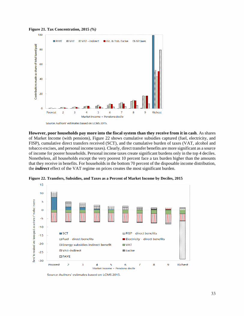
33

Figure 21. Tax Concentration, 2015 (%)

However, poor households pay more into the fiscal system than they receive from it in cash. As shares

of Market Income (with pensions), Figure 22 shows cumulative subsidies captured (fuel, electricity, and

FISP), cumulative direct transfers received (SCT), and the cumulative burden of taxes (VAT, alcohol and

tobacco excises, and personal income taxes). Clearly, direct transfer benefits are more significant as a source

of income for poorer households. Personal income taxes create significant burdens only in the top 4 deciles.

Nonetheless, all households except the very poorest 10 percent face a tax burden higher than the amounts

that they receive in benefits. For households in the bottom 70 percent of the disposable income distribution,

the indirect effect of the VAT regime on prices creates the most significant burden.

Figure 22. Transfers, Subsidies, and Taxes as a Percent of Market Income by Deciles, 2015

34

A move by the government to directly compensate poorer households would help fiscal policy achieve

poverty reduction and avoid fiscal impoverishment. Subsidy spending provides benefits directly and

indirectly to poor and rich households alike. Because the 2015-era coverage level for the social cash transfer

was low, energy subsidization delivered the only cash benefit generated from public expenditures for many

poor households. Using the fiscal incidence framework described in this report, we have estimated the

impacts on actual poverty and inequality levels if subsidy spending is reduced with SCT transfer spending

is increased. The table below demonstrates that partially or fully eliminating subsidy spending while using

a portion of that foregone expenditure to increase SCT coverage and benefit levels could reduce poverty by

as much as 4 percentage points, or could bring approximately 700,000 Zambians out of poverty.

Table 4. Fiscal Reforms and Poverty, Inequality Impacts

@ Disposable Income @ Consumable Income

Poverty

Headcount

Poverty

Gap Inequality

Poverty

Headcount

Poverty

Gap Inequality

Current/2015 54.4% 0.26 0.546 56.3% 0.28 0.543

Partial 53.9% 0.25 0.539 56.0% 0.27 0.534

Full 50.3% 0.24 0.539 53.3% 0.25 0.537 Source: Authors’ estimates based on LCMS 2015.

Notes: “Partial” reform includes the elimination of fuel and electricity subsidies and an increase in coverage of the SCT program

to 500,000 beneficiaries, and a 28 percent increase in SCT benefit levels. The increased SCT cost under “partial” reform represents

7 percent of foregone energy subsidy expenditures. “Full” reform includes the elimination of fuel, electricity, and FISP subsidies

and an increase in coverage of the SCT program to 500,000 beneficiaries, and a 100 percent increase in SCT benefit levels. The

increased SCT cost under “full” reform represents 18 percent of foregone energy and FISP expenditure.

CONCLUSIONS AND IMPLICATIONS

Fiscal policy in Zambia reduces inequality across a broad class of fiscal policy elements. Poorer

households receive a greater-than-proportional share of the government’s flagship direct transfer (the SCT

program). Direct taxes also are distributed progressively in that richer households are liable for tax shares

greater than their income shares. Subsidy spending is approximately proportional to income and therefore

does not much reduce or increase inequality. Indirect taxes overall reduce inequality.

Eliminating subsidy spending and moving to directly compensate poorer households would help fiscal

policy achieve poverty reduction and even greater inequality reduction. Because the 2015-era coverage

level for the social cash transfer was low, for many poor households, energy subsidy expenditures delivered

their only cash benefit generated from public expenditures. If subsidies on fuel, electricity, and agricultural

inputs were eliminated entirely while SCT program coverage was increased to 500,000 beneficiaries while

the benefit level was increased by 100 percent over its 2015 level, the poverty headcount ratio would be

expected to drop by approximately 4 percentage points (at Disposable Income) while inequality (as

measured by the Gini coefficient) would fall an additional 0.5 points. This SCT reform would require

resources equivalent to approximately 18 percent of the foregone subsidy expenditures.

Without reform, poor households will continue to pay more into the fiscal system than they receive

from it in cash. As we have shown, the share of subsidies on electricity, fuel, and agricultural inputs among

poor households is small while the benefit received is also small (relative to own income). Meanwhile, an

average household outside of the bottom 10 percent of the pre-fiscal income distribution faces a tax burden

from VAT, alcohol and tobacco excises, and personal income taxes higher than the amounts that are

received as direct or indirect benefits from subsidies or direct transfers. As a result, the number of poor and

vulnerable individuals who experience net cash subtractions from their incomes is greater than the number

of poor and vulnerable individuals who experience net additions. This dynamic creates impoverishment

among nearly 90 percent of the poor and vulnerable.

35

The FISP program should reform its standard operating procedure in order to better target poor

households. Particular FISP features – that access to subsidized inputs is controlled via cooperatives, for

example, or the requirement on land holdings – limit its coverage among very poor or remote households.

FISP targets poor households (at least those poor households who are involved in agriculture) better than

other subsidies, but the amount of program expenditure necessary to provide one FISP subsidy to a

household in the bottom 10 percent does not compare favorably to, for example, the SCT transfer.

VAT exemptions reduce the indirect tax burden for all households but cannot eliminate an indirect

tax burden in targeted households. Zambia in 2015 exempted over 80 percent of the average household’s

consumption basket (according to LCMS 2015).35 However, VAT exemptions imply that some portion of

value-added is not taxed. For example, producers of transport services still pay VAT charges on any non-

exempt inputs and, it is assumed, pass those input-VAT charges on to the final price of transport services.

As Figure 22 demonstrates, these indirect burdens are actually greater than direct VAT payments (on non-

exempt goods) for all but the very richest households. What this means, in essence, is that VAT-exempted

items are relatively important consumption-basket items for all households regardless of income levels.

Rather than exempting consumption categories from VAT, a more efficient way to deliver net benefits to

poor and vulnerable households is through targeted cash transfers at a scale large enough to compensate for

the burden created across households by VAT indirect taxes.

35 Most food, transport, education, health, and housing services are exempt from VAT.

36

REFERENCES

Arndt, C., K. Pauw, and J. Thurlow. 2014. “The Economywide Impacts and Risks of

Malawi’s Farm Input Subsidy Programme.” WIDER Working Paper No. 99/2014. Helsinki,

Finland: United Nations University, World Institute for Development Economics Research.

Bhorat, H., M. Oosthuizen, D. Yu, and N. Kachingwe. (2016). “Understanding Growth-Income Inequality

Interactions in Zambia.” Development Policy Research Unit, University of Cape Town. Mimeo.

Bollinger, Christopher and Barry Hirsch. 2007. “How Well are Earnings Measured in the Current

Population Survey? Bias from Nonresponse and Proxy Respondents,” Working Paper.

Bollinger, Christopher and Barry Hirsch. 2013. “Is Earnings Nonresponse Ignorable?” Journal of Labor

Economics, (24)3.

Burke, William J., T.S. Jayne, and J. Roy Black. 2012. “Getting More `Bang for the Buck’: Diversifying

Subsidies Beyond Fertilizer and Policy Beyond Subsidies.” Policy Synthesis Food Security Research

Project No. 52. Ministry of Agriculture and Livestock, Agricultural Consultative Forum: Michigan State

University and Lusaka, Zambia. ahttp://aec.msu.edu/fs2/zambia/index.htm

Central Statistics Office. 2016. “2015 Living Conditions and Monitoring Survey (LCMS) Report,”

Lusaka, Zambia.

Central Statistics Office (Zambia CSO) and World Bank. 2016. “The Methodology for Consumption-

Poverty Estimation in Zambia in 2015.”

Cuesta, J., P. Kabaso, and P. Suarez-Becerra. 2012. “How Pro-Poor and Progressive Is Social Spending in

Zambia?” Policy Research Working Paper 6052. Washington, DC: World Bank.

Dabalen, A., A. Narayan, J. Saavedra-Chanduvi, A. Hoyos Suarez, A. Abras, and S. Tiwari. 2015. Do

African Children Have an Equal Chance? A Human Opportunity Report for Sub-Saharan

Africa. Directions in Development–Poverty. Washington, DC: World Bank.

Jellema, Jon R., Nora Lustig, Astrid Haas, and Sebastian Wolf. 2016. “The Impact of Taxes, Transfers,

and Subsidies on Inequality and Poverty in Uganda.” Commitment to Equity Institute Working Paper No.

53.

Higgins, Sean and Nora Lustig. 2016. “Can a poverty-reducing and progressive tax and transfer system

hurt the poor?” Journal of Development Economics, 122(C).

Lustig, Nora, ed. 2016. Commitment to Equity Handbook: Estimating the Redistributive Impact of Fiscal

Policy. Washington, DC and New Orleans: Brookings Institution and CEQ Institute/Tulane University.

Jayne, T.S., Nicole M. Mason, William J. Burke, and Joshua Ariga. 2016. “Agricultural Input Subsidy

Programs in Africa: An Assessment of Recent Evidence.” Michigan State University International

Development Working Paper No. 145 to Equity Institute Working Paper No. 53.

Mason, N.M. T.S. Jayne, and R. Mofya-Mukuka. 2013. “Zambia’s Input Subsidy Programs.” Agricultural

Economics 44(6).

McIntyre D., and F. Meheus. 2014. Fiscal Space for Domestic Funding of Health and Other Social

Services. London: Chatham House.

37

Peters, David H., Sameh El-Saharty, Banafsheh Siadat, Katja Janovsky, and Marko Vujicic. 2009.

Improving Health Service Delivery in Developing Countries: From Evidence to Action. Directions in

Human Development. Washington, DC: World Bank.

Republic of Zambia. 2015. Budget Address. Ministry of Finance, Republic of Zambia, Lusaka.

http://www.mof.gov.zm/index.php/budgetdata/summary/15-budget-speeches/262-budget-speech-2015

_____. 2016. Budget Address. Ministry of Finance, Republic of Zambia, Lusaka.

http://www.mof.gov.zm/index.php/budgetdata/summary/15-budget-speeches/9751-budget-speech-2016

_____. 2016. 2015 Annual Economic Report. Ministry of Finance, Republic of Zambia, Lusaka.

http://www.mof.gov.zm/index.php/economicdata/summary/59-annual-economic-reports/11377-2015-

economic-report

MoH (Ministry of Health), Republic of Zambia. 2016. Ministry of Finance, Republic of Zambia, Lusaka.

Still need to check this source.

Ricker‐Gilbert, J., N.M. Mason, F.A. Darko, and S.T. Tembo. 2013. What Are the Effects of Input Subsidy

Programs on Maize Prices? Evidence from Malawi and Zambia. Agricultural Economics 44 (6): 671–86.

Smith, Gregory, Fiona Davies, and Zivanemoyo Chinzara. 2016. “Beating the Slowdown in Zambia.”

World Bank Operational Studies 25270. Washington, DC: World Bank.

Trimble, Chris, Masami Kojima, Ines Perez Arroyo, and Farah Mohammadzadeh. 2016. Financial

Viability of Electricity Sectors in Sub-Saharan Africa: Quasi-Fiscal Deficits and Hidden Costs. World

Bank Policy Research Working Paper 7788. Washington, DC: World Bank.

WDI (World Development Indicators). 2015. World Bank, Washington, DC.

http://data.worldbank.org/data-catalog/world-development-indicators

WHO (World Health Organization). 2015. Global Health Expenditure database. Geneva.

http://www.who.int/health-accounts/ghed/en/

World Bank. 2015. Education Public Expenditure Review in Zambia. Washington, DC: World Bank.

Chikuba, Zai, Malunga Syacumpi; and James Thurlow. 2013. A 2007 Social Accounting Matrix (SAM)

for Zambia. Washington, DC: Zambia Institute for Policy Analysis and Research and International Food

Policy Research Institute (IFPRI). https://www.ifpri.org/publication/2007-social-accounting-matrix-sam-

zambia.