pursuing photovoltaic cost-effectiveness

IEEE Industry Applications Magazine � september/october 2017 1077-2618/17©2017Ieee40

Countries with a Considerable number of photovoltaic (PV) installations are facing the challenge of overloading their power grid during peak power produc-tion hours if the power infrastructure remains the same. to address this, regulations have been imposed on PV sys-tems to ensure that more active and flexible power control is performed. as an advanced control strategy, absolute active power control (aaPC) can effectively solve overload-ing issues by limiting the maximum possible PV power to a certain level (i.e., the power limitation) and can also benefit the inverter reliability because of the reduced ther-mal loading of the power devices. however, its feasibility

is challenged by the associated energy losses. an increase in the inverter lifetime and a reduction of the energy yield can alter the cost of energy, demanding an optimization of the power limitation. therefore, aiming at minimizing the levelized cost of energy (lCoe), this article discusses how to optimize the power limit for the aaPC strategy.

the optimization method is demonstrated on a 3-kw, single-phase PV system with a real-field mission profile (i.e., solar irradiance and ambient temperature). the opti-mization results reveal that enabling the aaPC strategy pro-vides superior performance in terms of lCoe and energy production compared to the conventional PV inverter operating only in the maximum power point tracking (mPPt) mode. in the presented case study, the mini-mum of the lCoe is achieved for the PV system when

By Yongheng Yang, Eftichios Koutroulis,

Ariya Sangwongwanich, and Frede Blaabjerg

Pursuing Photovoltaic Cost-Effectiveness

©istockphoto.com/ urfinguss

Digital Object Identifier 10.1109/MIAS.2016.2600722 Date of publication: 26 June 2017

ABSOLUTE ACTIVE POWER CONTROL OFFERS HOPE IN SINGLE-PHASE PV SYSTEMS

september/october 2017 � IEEE Industry Applications Magazine 41

the power limit is optimized to a certain level of the designed maximum feed-in power (i.e., 3 kw). in addi-tion, the lCoe-based analysis method can be used in the design of PV inverters considering long-term mission profiles.

Studies to Datesolar PV installations are still growing at a spectacular rate worldwide [1]. thus, challenging issues occasionally appear, such as overloading of the distributed grid due to the peak power generation of PV systems [2]–[4]. in the case of the large-scale adoption of PV systems, advanced control strategies, e.g., power-ramp control and absolute power control, which are currently required for wind power systems in different countries, have been used to strengthen PV systems [3]–[12]. in the danish grid code [7], a constant power generation (CPG) control concept for PV systems by limiting the maximum feed-in power was proposed to solve the overloading issues in peak power production periods [6].

other methods have also been developed in the lit-erature. however, either increased total cost or control complexity has been observed in prior solutions. for instance, expanding the grid capacity (i.e., grid reinforce-ment) will incur an additional investment, and integrating energy storage systems to handle the peak power not only increases the control complexity but also lowers the entire system reliability [13]–[15]. in contrast, the aaPC scheme requires only minor software modifications when implemented, as it is a feasible and cost-effective strategy [12], [14]–[19]. this explains why such power control is receiving attention in some countries, such as Germany, denmark, and Japan [7], [9], [11].

in addition, aaPC feasibility in grid-connected PV applications has been investigated in [6] and [14] in terms of a rough estimation of the energy losses and the PV inverter lifetime, respectively, where the aaPC scheme is also referred to as a CPG control. the scheme, having a reasonable power limitation (e.g., 80%), does not annu-ally result in a substantial energy yield reduction [3], [6]. as a consequence of applying the aaPC strategy, a reduction of the thermal stresses on the power devices, e.g., insulated-gate bipolar transistors, has been achieved because the power losses inducing temperature rises will be changed when the PV system enters into the aaPC mode from the mPPt mode, and vice versa. therefore, a hybrid control method (mPPt–aaPC) will also contribute to improved reliability and extend the lifetime of the PV system beyond resolving the overloading issues [6], [14].

notably, both the energy production and the system lifetime are the main indicators of the lCoe, which has become the key to increasing the competitiveness of PV systems compared with other renewables [20]–[22]. many efforts have been devoted to the design and control of PV systems, with a common goal of reducing the cost of energy (i.e., producing a lower lCoe) [23]–[25]. for

instance, a circuit-level design of a PV inverter that con-siders the failure rate of the circuit devices (calculated according to [26]) was presented in [22]. furthermore, methods such as adopting highly efficient transformer-less PV inverters and reliability-oriented designs have been seen in recent applications [22]–[24], [27]–[32]. trans-formerless PV inverters can somehow increase energy production because of their high efficiency [28], [32], [33]. however, the mPPt–aaPC operational mode goes against the objective of maximizing the energy production of PV systems, although the capped energy is quite limited throughout the year [3], [6]. the improved reliability (i.e., the extended service time) of PV systems can compensate for such a loss to some extent, as long as the power limit is appropriately designed.

in that regard, this article serves to find the optimal power limitation level for the mPPt–aaPC scheme with a target of minimizing the lCoe considering long- term mission profiles (i.e., solar irradiance and am bient temperature).

Absolute Active Power Control

The Hybrid Power Control Methodfigure 1 shows the configuration of a single-phase, dou-ble-stage, grid-connected PV system with the hybrid power control and a general control structure of the boost converter stage. although there are several aaPC pos-sibilities to achieve a CPG when the available PV power ppv exceeds the power limit ,P limit modifying the mPPt control has been adopted from the viewpoint of simplic-ity and cost-effectiveness [19], [34]. figure 1 shows that the aaPC scheme is implemented in the control of the boost converter. as mentioned previously, the PV inverter can be transformerless to maintain a high efficiency, and thus a full-bridge inverter topology with a bipolar modulation scheme is adopted in figure 1. when considering the quality of the injected grid current ,ig an inductor-capac-itor-inductor (lCl) filter has been employed as the inter-mediate component between the full-bridge PV inverter and the grid.

with respect to the aaPC scheme in this article, the operating principle of a PV system with a hybrid control scheme (mPPt–aaPC) can be described as follows. when the available PV output power ppv exceeds the power limitation ,P limit the system should go into the aaPC mode. in that case, the PV output reference voltage v*pv is continuously perturbed toward certain points (e.g., points a and b in figure 2) at which a CPG operation of the PV panels is achieved. once ,Pppv limit1 the PV system oper-ates in the mPPt mode with a peak power injection to the grid from the PV panels (i.e., the energy harvesting is maximized). this can be further described as

whenwhen

,vvv v

PP p PP p P

* mpp

mpp

mpp it

it it

lim

lim limpv pv

pv

pv&

!

1$D

= =) ) (1)

IEEE Industry Applications Magazine � september/october 201742

where vD is the perturbation step size to achieve an aaPC operation, ppv is the PV instantaneous (available) power, Ppv is output power of the PV panels, and vmpp and Pmpp are the PV voltage and power, respectively, at the mPP. in both operational modes, a proportional integrator (Pi) controller is employed to regulate the PV output volt-age vpv through controlling the boost converter, as shown in figure 1.

figure 3 demonstrates the performance of a 3-kw sin-gle-phase double-stage PV system with the mPPt–aaPC scheme under a trapezoidal solar irradiance profile. the figure shows that the adopted control scheme [as illustrat-ed in figure 1(b) and (1)] can effectively achieve the con-stant power production of the PV system as well as smooth and stable operation mode transients, in contrast to the prior-art solutions [6], [16]–[18]. in this case, the PV system is operating in the region of low /dP dvpv pv according to the power–voltage characteristic of PV panels, as demon-strated in figure 2. the operating point in the aaPC mode of figure 3 was controlled at the left side of the mPP (i.e., point a in figure 2). however, it can also operate at the right side of the mPP (i.e., point b in figure 2) at the cost of increased power losses (because of power variations) due to the high /dP dvpv pv in that region [6]. moreover, the PV system may become unstable in that case [34]. hence, in this article, the aaPC operating point is regulated at the left side of the mPP, which is also enabled by the double-stage configuration [i.e., figure 1(a)].

Mission Profile Translationa mission profile is normally referred to as a simplified rep-resentation of relevant conditions under which the con-sidered system is operating [35]–[37]. for grid- connected PV systems, the mission profile includes the solar irradi-ance and the ambient temperature of certain locations where the PV systems are installed, and it can be taken as a reflection of the intermittent nature of the solar PV

PV Panels

°C

ipv

ipv

Vpv

Vpv

Vdc

Vdc Vinv Vg

Vg

ig

ig

ωt

Zg

Ppv

Plimit

L

Boost Converter

PWMb

PWMinv

MPPT–AAPC

Vdc∗

Cdc

PLL

Inverter Control

InverterLCL Filter Grid

L1 L2

+

ipv Vpv

Plimit MPPT–AAPCVpv

∗

+– PI PWMb

Duty Cycle

Boost Converter

(a)

(b)

Cf

FIGURE 1. A single-phase, double-stage, grid-connected PV system with an LCL filter: (a) a hardware schematic and overall control structure and (b) a control block diagram of the boost converter with the MPPT-AAPC scheme. PWM: pulsewidth modulation; PLL: phase-locked loop.

3

2.5

2

1.5

1

0.5

0 50 100 150 200 250 300 350PV Voltage (V)

Low dPpv/dvpv Hig

h dP

pv/d

v pv

PV

Out

put P

ower

(kW

)

dvpv

dPpv

A B

MPP2.4 kW

(80% of Rated)

Plimit = 2.4 kW

FIGURE 2. The power–voltage characteristic of a PV array (solar irradiance: 1,000 W/ ;m2 ambient temperature: 25 °C), where the power limit of 80% of the rated power (i.e., . kWP 2 4itlim = ) is also shown.


energy. thus, the mission profile becomes an essential part of the PV-inverter reliability analysis. specifically, to perform the reliability analysis of the PV inverter, the mission profile inevitably must be translated to the power losses and then the thermal loading in a long-term opera-tion (e.g., a yearly operational profile) [31], [32], [35], [38], [39]. if not appropriately handled, the analysis can be very time consuming because of the large amount of data. accordingly, a time-efficient and cost-effective mission pro-file translation method is introduced.

figure 4 illustrates details of the mission profile translation approach, with which the power losses and thermal loading of the power devices under any given mission profile can be obtained. a number of cases under constant environmental conditions (e.g., an ambient temperature of 25 °C and a solar irradiance level of , W/m )1 000 2 were first translated according to figure 4(a)

to build up the lookup-table-based loss and thermal models. subsequently, a long-term mission profile, even with a high sampling rate, can be directly translated to the total power losses (and also energy production) and the thermal loading of the power devices, which are then used for lCoe analysis.

The LCOE of PV Invertersthe PV inverter lCoe (€/wh) is a function of the PV inverter power rating Pr [20], [27]. it can be expressed as

,PE PC P

LCOE ry r

rinv=^ ^

^h hh

(2)

in which ( )Cinv $ (€) is the present total cost of the PV inverter during its lifetime and ( )Ey $ (wh) is the total energy injected into the grid by the PV inverter over its life span. where the PV inverter operates in the aaPC mode, its nominal power rating is constrained to ,P P itlimr = as discussed in the section “the hybrid Power Control method.” in the mPPt mode, it holds that ,P Pnr = with Pn being the inverter nominal power designed at standard test conditions (stC), i.e., a solar irradiance of 1 kw/m ,2 a solar cell temperature of 25 °C, and an air mass of 1.5. thus, in the mPPt mode, the

input power of the inverter is curtailed at Pn (i.e., the PV inverter is normally undersized [40], [41]), while in the aaPC mode, the power limit for curtailment is P itlim (i.e., to maintain a constant power production).

in (2), the present total cost of the PV inverter depends on the corresponding manufacturing and maintenance costs [27]:

( ) ( ) ( ),C P C P M Pinv r m r c r= + (3)

where ( )Cm $ (€) is the PV inverter manufacturing cost and ( )M Pc r (€) is the present value of the total maintenance

MissionProfile

MissionProfile

Electrical and Control Domain Thermal Domain

Thermal Model

PV Model

PV Inverter

MPPT–AAPC

Grid

Pin PoutPloss

PlossPloss

Tj

Tj Tj

PowerLosses

ThermalLoadingProfile

PowerLosses

ThermalLoadingProfile

Lookup-Table-BasedSimulation Model

(a) (b)

°C °C

FIGURE 4. An approach to translate mission profiles to power losses P loss and thermal loading (i.e., device junction temperature Tj): (a) for short-term mission profiles and (b) for long-term mission profiles.

3.5

3

2.5

2

1.5

1

0.5

0

PV

Pow

er (

kW)

3.5

3

2.5

2

1.5

1

0.5

0

PV

Pow

er (

kW)

10:43:37

200 250 300 350 400PV Voltage (V)

(b)

MPPTOperation

Actual OperationalTrajectory with the

AAPC Scheme

450

10:45:17 10:46:57 10:48:37 10:50:17Time (hh:mm:ss)

(a)

2.4 kW(80% of Rated)

Available PV Power

Plimit = 2.4 kW

Plimit = 2.4 kW

Actual PVOutput Power

MPPT AAPC MPPT

Ideal OperationalTrajectoryAAPC Operation

FIGURE 3. An operational example (experiments) of a 3-kW single-phase, double-stage PV system with the MPPT-AAPC scheme, where the power limit is set to be 80% of the rated power (i.e.,

. kWP 2 4itlim = ) and the ambient temperature is around 25 °C: (a) PV output power and (b) operational trajectories.


cost of the PV inverter through its lifetime. further-more, the PV inverter manufacturing cost is propor-tional to Pr:

( ) ,C P c P Cm r m r 0= + (4)

with cm being the proportionality factor (€/kw) and C0 the initial cost, which is considered zero in this article since it is much lower than the total cost of the PV inverter.

as a consequence, in the aaPC mode, the PV inverter cost is proportional to the preset power limit ,P itlim while in the mPPt mode, the inverter cost is proportional to the nominal power rating Pn that is designed at stC. the total maintenance cost ( )Mc $ depends on the PV inverter reliability features, which, in turn, depend on the power rating of the PV inverter. in the proposed methodology, the lifetime in years of the PV inverter power devices is initially calculated. it is assumed that each time the PV inverter power devices’ end of life is reached, mainte-nance on the PV inverter will be performed, imposing the corresponding maintenance cost. therefore, the present value of the total maintenance cost of the PV inverter

( )M Prc is calculated by reducing the (future) expenses occurring at the end of the power devices’ lifetime for repairing the PV inverter to the corresponding present value, as follows:

( )( )

,M P LF P R Pdg

11

· · ·c r j r c r j

j

j

n

1

=+

+

=

^ ^h h/ (5)

in which n is the PV system’s operational lifetime (e.g., 30 years), Rc (€/kw) is the present value of the PV inverter repair cost per kilowatts of the power rating, g (%) is the annual inflation rate, d (%) is the annual discount rate, and (·)LFj is the inverter lifetime, with

.j n1 # # if the lifetime of the power devices expires at the j th year of operation, ( ) ;LF P 1j n = otherwise,

( ) .LF P 0j n = notably, the repair cost Rc in (5) consists of both the purchase cost of the failed power devices and the potential labor and transportation expenses for repairing/replacing the PV inverter. the previous discussion, in the section “the hybrid Power Control method,” confirms that the aaPC control method will affect the lCoe (i.e., the cost of the PV energy).

the following demonstrates how to calculate the lCoe of only the PV inverter [as shown in (2)], considering the long-term mission profile effect on the inverter lifetime, where the grid fundamental-frequency thermal cycles are not considered at this stage. however, the PV panel cost also accounts for a major share of the total cost of the entire grid-connected PV system [20], [27], including other components such as capacitors and printed circuit boards for implementing the control algorithms. this becomes the main limitation of the presented lCoe optimization method, and it will affect the design results. nevertheless, the lCoe analysis approach and the optimization of the aaPC control power limitation can be of much value in assessing and designing multiple PV systems.

Minimized LCOE (Case Study Results)

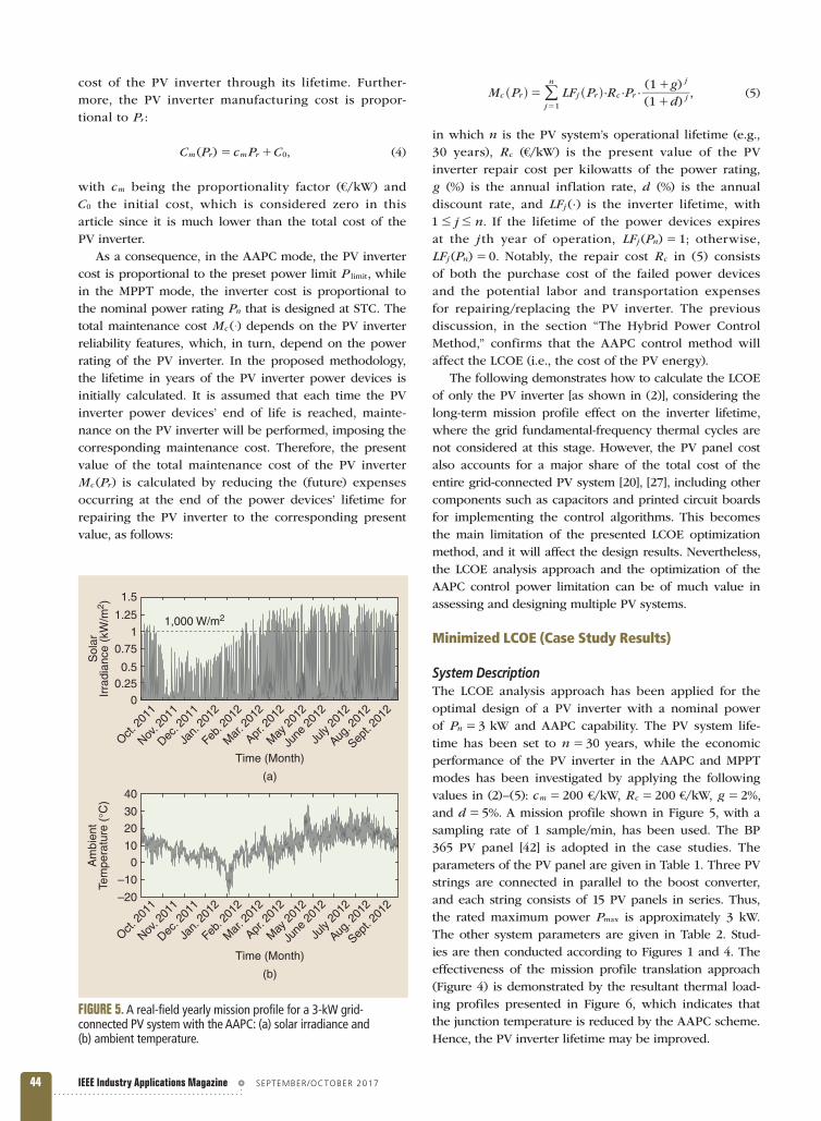
System Descriptionthe lCoe analysis approach has been applied for the optimal design of a PV inverter with a nominal power of P 3n = kw and aaPC capability. the PV system life-time has been set to n 30= years, while the economic performance of the PV inverter in the aaPC and mPPt modes has been investigated by applying the following values in (2)–(5): c 200m = €/kw, R 200c = €/kw, %,g 2= and %.d 5= a mission profile shown in figure 5, with a sampling rate of 1 sample/min, has been used. the bP 365 PV panel [42] is adopted in the case studies. the parameters of the PV panel are given in table 1. three PV strings are connected in parallel to the boost converter, and each string consists of 15 PV panels in series. thus, the rated maximum power Pmax is approximately 3 kw. the other system parameters are given in table 2. stud-ies are then conducted according to figures 1 and 4. the effectiveness of the mission profile translation approach (figure 4) is demonstrated by the resultant thermal load-ing profiles presented in figure 6, which indicates that the junction temperature is reduced by the aaPC scheme. hence, the PV inverter lifetime may be improved.

1.5

1.25

0.75

0.50.25

40

30

20

10

–10

–20

0

Sol

arIr

radi

ance

(kW

/m2 )

Am

bien

tTe

mpe

ratu

re (

°C)

0

1

Oct. 2

011

Nov. 2

011

Dec. 2

011

Jan.

2012

Feb.

2012

Mar

. 201

2

Apr. 2

012

May

201

2

June

201

2

July

2012

Aug. 2

012

Sept. 2

012

Oct. 2

011

Nov. 2

011

Dec. 2

011

Jan.

2012

Feb.

2012

Mar

. 201

2

Apr. 2

012

May

201

2

June

201

2

July

2012

Aug. 2

012

Sept. 2

012

Time (Month)

(b)

Time (Month)

(a)

1,000 W/m2

FIGURE 5. A real-field yearly mission profile for a 3-kW grid-connected PV system with the AAPC: (a) solar irradiance and (b) ambient temperature.


LCOE Analysisthe power losses can be obtained with the mission pro-file translation approach. Consequently, the energy yield can be calculated under different power limits ,P limit as illustrated in figure 7. in these simulations, the energy production has been normalized to the corresponding energy production in the mPPt mode. due to the limita-tion of feed-in power in the aaPC mode, the resultant energy production shown in figure 7 is lower than that in the mPPt mode for %P 0 110itlim = - of the rated power

.Pn however, when P itlim is higher than 120%, the energy production in the aaPC mode is higher than that pro-duced only in the mPPt mode, where the input power of the inverter is curtailed at the designed power rating ,Pn as shown in figure 7. this is because the PV panel rat-ing has been selected to be 3 kw at stC. since the mis-sion profile shown in figure 5 has some periods where the solar irradiance level is higher than , W/m ,1 000 2 the power production during those periods is higher than the designed ,Pn which is considered to be the power limitation in the mPPt mode (i.e., the PV system is actu-ally operating in the aaPC mode with a power limit of

P Pitlim n= ). thus, during those time intervals, the excess energy is lost when operating even in the mPPt mode.

lifetime estimation is not a direct outcome of the mis-sion profile-based analysis approach, which gives only the thermal loading profile for qualitative analysis. to calculate the lifetime (and then the lCoe), the thermal loading has to be interpreted properly according to specific lifetime models—i.e., the information (e.g., temperature cycle ampli-tude and mean junction temperature) in the random loading profile should be extracted by means of a counting algo-rithm such as a rain-flow counting process [43]–[45]. figure 8 illustrates the work flow of counting the thermal loading profiles (e.g., the loading profiles in figure 6). then, using the extracted information, the lifetime of the power devices can be estimated according to the lifetime model [46].

subsequently, the lifetime of the PV inverter, when oper-ating in the aaPC mode for various values of the power limitation ,P itlim is presented in figure 9. the figure shows that, for %,P 0 100itlim = - the PV inverter lifetime is higher than the operational lifetime of the PV system, thus guar-anteeing that no failure of the power devices will occur during that period. the corresponding present value of the

Table 2. The parameters of the single-phase, double-stage, grid-connected PV system shown in Figure 1

Parameter Symbol Value

Grid voltage amplitude vgn 325 V

Grid frequency 0~ 2 50#r rad/s

Boost converter inductor L 5 mH

dc-link capacitor Cdc , F2 200 n

Grid impedance LgRg

2 mH.20 X

LCL filter ,L L1 2

Cf

2 mH, 3 mH. F4 7 n

Sampling frequency fsw 10 kHz

Switching frequencies for both converters

,f finvb 10 kHz

Table 1. The parameters of the BP 365 solar PV panel at STC

Parameter Symbol ValueRated power Pmpp 65 W

Voltage at Pmpp Vmpp 17.6 V

Current at Pmpp Impp 3.69 A

Open-circuit voltage Voc 21.7 V

Short circuit current Isc 3.99 A Time (Month)

with AAPC Scheme

Without AAPC Scheme(i.e., MPPT Operation)

80

60

40

20

0

–20

Junc

tion

Tem

pera

ture

(°C

)

Oct. 2

011

Nov. 2

011

Dec. 2

011

Jan.

2012

Feb.

2012

Mar

. 201

2

Apr. 2

012

May

201

2

June

201

2

July

2012

Aug. 2

012

Sept. 2

012

FIGURE 6. Thermal loading (simulation results) of the power devices of the PV inverter with and without the AAPC ( . kWP 2 4limit = , i.e., 80% of the nominal power) under the yearly mission profile (Figure 5).

120

100

80

60

40

20

00 25 50 75 100

Power Limit (% of the Rated Power)

Nor

mal

ized

Ene

rgy

Pro

duct

ion

(%)

125 150

High Energy Production

Low Energy Production

FIGURE 7. The energy production simulation results of the 3-kW single-phase PV system in the MPPT–AAPC mode, according to the mission profile shown in Figure 5, which has been normalized to the corresponding energy production only in the MPPT mode for various values of the power limit P limit.


lifetime maintenance cost in the aaPC mode for various values of the power limitation P itlim is shown in figure 10. figure 9 also shows that, when the power limit P itlim reaches the range of 100–150% of the rated power, the PV inverter lifetime in the aaPC mode is progressively reduced to approxi-mately 21 years, corres ponding to one repair of the PV inverter during the PV system lifetime, and the mainte-nance cost is increased according to (5), as shown in figure 10. in con-trast, according to figures 7 and 9, the PV inverter lifetime with the same or higher energy production is approxi-mately 21 years, resulting in one inverter repair during the lifetime of

the PV system, which corresponds to Mc = €326.4.the total cost of the PV inverter operating in the mPPt–

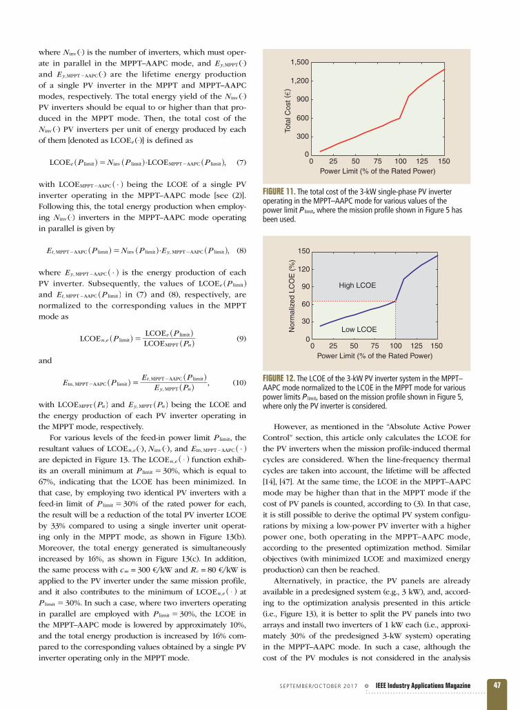
aaPC mode, including the manufacturing and maintenance expenses, according to (3), is plotted in figure 11. for values of the power limit P itlim in the range of 0–100% of the rated power, the maintenance cost is zero, as shown in figure 10. hence, the total cost depends only on the inverter construction cost, which is proportional to the power limit P itlim , according to (4). however, when P itlim > 100%, the total cost in the mPPt–aaPC mode is affected by both construction and maintenance expenses, as indicated in figure 11. in the operating mode of maximum power production, the total cost of the inverter is equal to Cinv = €926.4. although the lifetime energy production is higher in that case, as analyzed previously, the PV inverter cost is also higher in this operating mode when P 100itlim 2 % of ,Pn as shown in figure 11.moreover, the lCoes of a 3-kw PV inverter in the

mPPt–aaPC and mPPt modes, respectively, have been calculated using (2) for various values of the power limit P itlim to find the optimal power limitation under the mission profile shown in figure 5. the results are pre-sented in figure 12, which shows that the lCoe value in the mPPt–aaPC mode is always less than that in the only-mPPt mode (i.e., the conventional operational mode at unity power factor) but also that the energy production is less in the case of mPPt–aaPC operation, as discussed previously.

as a consequence, in practical applications, to achieve a total energy generation equal to or higher than that in the mPPt mode, multiple identical PV inverters would be reasonably considered a requirement to operate in paral-lel in the mPPt–aaPC mode, each of them having a feed-in power limitation of P itlim . in this case, the total number of inverters is given by

,N PE P

E Pinv it

,MPPT AAPC it

,MPPTlim

limy

y n=

-^ ^

^h hhc m (6)

Thermal LoadingProfile

Thermal Loading Interpretation

Counting Algorithms

• Level Crossing• Rain Flow• Simple Range Counting• Etc.

Thermal Information

• Tjm (Mean Junction Temperature)• ∆Tj (Temperature Cycle Amplitude)• ton (Cycle Period)• Etc.

Loading ProfileCounting

LifetimeModels

FIGURE 8. A thermal loading interpretation work flow of the loading profiles for lifetime estimation.

104

103

102

101

Est

imat

ed L

ifetim

e (Y

ears

)

0 25 50 75 100 125 150Power Limit (% of the Rated Power)

30 Years

FIGURE 9. The lifetime of the 3-kW single-phase PV inverter when operating in the MPPT–AAPC mode for various power limits P limit, considering the mission profile effect (the mission profile shown in Figure 5 has been used).

500

400

300

200

100

00 25 50 75 100 125 150


MaintenanceRequired

Pre

sent

Mai

nten

ance

Cos

t)

(

FIGURE 10. The present value of the lifetime maintenance cost of the 3-kW single-phase PV inverter when operating in the MPPT–AAPC mode for various values of the power limit ,P itlim considering the mission profile presented in Figure 5.


where ( )Ninv $ is the number of inverters, which must oper-ate in parallel in the mPPt–aaPC mode, and ( )E ,MPPTy $ and ( )E ,MPPT AAPCy $- are the lifetime energy production of a single PV inverter in the mPPt and mPPt–aaPC modes, respectively. the total energy yield of the ( )Ninv $ PV inverters should be equal to or higher than that pro-duced in the mPPt mode. then, the total cost of the

( )Ninv $ PV inverters per unit of energy produced by each of them [denoted as ( )LCOEe $ ] is defined as

LCOE LCOE ,P N P P·it inv it MPPT AAPC itlim lim lime = -^ ^ ^h h h (7)

with LCOE ·MPPT AAPC- ^ h being the lCoe of a single PV inverter operating in the mPPt–aaPC mode [see (2)]. following this, the total energy production when employ-ing ( )Ninv $ inverters in the mPPt–aaPC mode operating in parallel is given by

,E P N P E P·, MPPT AAPC it inv it , MPPT AAPC itlim lim limt y=- -^ ^ ^h h h (8)

where E ·, MPPT AAPCy - ^ h is the energy production of each PV inverter. subsequently, the values of LCOE P itlime ^ h and E P, MPPT AAPC itlimt - ^ h in (7) and (8), respectively, are normalized to the corresponding values in the mPPt mode as

LCOELCOELCOE

PP

P, it

MPPT

itlim

limn e

e

n=^ ^

^h hh (9)

and

,E PE P

E P, MPPT AAPC it

, MPPT

, MPPT AAPC itlim

lim

y

t

ntn =-

-^ ^^h h

h (10)

with LCOE PMPPT n^ h and E P, MPPTy n^ h being the lCoe and the energy production of each PV inverter operating in the mPPt mode, respectively.

for various levels of the feed-in power limit ,P itlim the resultant values of LCOE ( ), ( ),N, invn e $ $ and E ·, MPPT AAPCtn - ^ h are depicted in figure 13. the LCOE ,n e $^ h function exhib-its an overall minimum at %,P 30itlim = which is equal to 67%, indicating that the lCoe has been minimized. in that case, by employing two identical PV inverters with a feed-in limit of %P 30itlim = of the rated power for each, the result will be a reduction of the total PV inverter lCoe by 33% compared to using a single inverter unit operat-ing only in the mPPt mode, as shown in figure 13(b). moreover, the total energy generated is simultaneously increased by 16%, as shown in figure 13(c). in addition, the same process with cm = 300 €/kw and Rc = 80 €/kw is applied to the PV inverter under the same mission profile, and it also contributes to the minimum of LCOE ,n e $^ h at

%.P 30itlim = in such a case, where two inverters operating in parallel are employed with %,P 30itlim = the lCoe in the mPPt–aaPC mode is lowered by approximately 10%, and the total energy production is increased by 16% com-pared to the corresponding values obtained by a single PV inverter operating only in the mPPt mode.

however, as mentioned in the “absolute active Power Control” section, this article only calculates the lCoe for the PV inverters when the mission profile-induced thermal cycles are considered. when the line-frequency thermal cycles are taken into account, the lifetime will be affected [14], [47]. at the same time, the lCoe in the mPPt–aaPC mode may be higher than that in the mPPt mode if the cost of PV panels is counted, according to (3). in that case, it is still possible to derive the optimal PV system configu-rations by mixing a low-power PV inverter with a higher power one, both operating in the mPPt–aaPC mode, according to the presented optimization method. similar objectives (with minimized lCoe and maximized energy production) can then be reached.

alternatively, in practice, the PV panels are already available in a predesigned system (e.g., 3 kw), and, accord-ing to the optimization analysis presented in this article (i.e., figure 13), it is better to split the PV panels into two arrays and install two inverters of 1 kw each (i.e., approxi-mately 30% of the predesigned 3-kw system) operating in the mPPt–aaPC mode. in such a case, although the cost of the PV modules is not considered in the analysis

1,500

1,200

900

600

300

00 25 50 75 100 125 150


Tota

l Cos

t)

(

FIGURE 11. The total cost of the 3-kW single-phase PV inverter operating in the MPPT–AAPC mode for various values of the power limit P limit, where the mission profile shown in Figure 5 has been used.

150

120

90

60

30

00 25 50 75 100


Nor

mal

ized

LC

OE

(%

)

125 150

High LCOE

Low LCOE

FIGURE 12. The LCOE of the 3-kW PV inverter system in the MPPT–AAPC mode normalized to the LCOE in the MPPT mode for various power limits P limit, based on the mission profile shown in Figure 5, where only the PV inverter is considered.


here (they should be paid for by both the 3-kw system in the mPPt mode and the two 1-kw systems in the mPPt–aaPC mode), the investigation in this article is valid in terms of minimizing lCoe while maintaining a higher energy production.

Conclusionsthe lCoe of PV inverters with an aaPC scheme has been calculated and analyzed in this article within the context of a long-term, real-field mission profile. the analysis has

revealed that the hybrid power control (i.e., a mixture of the mPPt and aaPC operational modes, mPPt–aaPC) can contribute to an improved lifetime of the power devices because of the reduced thermal loading. however, a reduction of energy production is associated with this reliability benefit. this article demonstrates that, by opti-mizing the power limit imposed on multiple PV inverters operating in the hybrid mPPt–aaPC mode, a minimized lCoe can be obtained. simultaneously, an increase of the PV-generated energy is achieved compared to the use of a single PV inverter operating in only the mPPt mode.

most importantly, the presented optimization method and the lCoe analysis can be an effective design tool for PV system planning (e.g., with a cluster of PV inverters) when the mission profile (both long-term and line- frequency thermal cycles) and the PV panel cost are also considered. specifically, by applying the last part of the optimization design in this article (i.e., related to figure 13), the opera-tion of each inverter in the cluster of the PV systems can be optimally selected in such a way that 1) an overall constant power production is achieved, 2) the total energy produc-tion is not reduced, and 3) the lCoe is minimized.

Acknowledgmentsthis work was supported by the european Commis-sion through the european union’s seventh framework Program (fP7/2007–2013) through the solar-era.net transnational Project (PV2.3-PV2Grid), by energinet.dk (forskel, denmark, Project 2015-1-12359), and by the research Promotion foundation (rPf, Cyprus, Project Koina/solar-era.net/0114/02).

Author InformationYongheng Yang ([email protected]), Ariya Sangwong-wanich, and Frede Blaabjerg are with aalborg university, denmark. Eftichios Koutroulis is with the technical uni-versity of Crete, Chania, Greece. Yang is a member of the ieee. Koutroulis is a senior member of the ieee. blaabjerg is a fellow of the ieee. this article first appeared as “mini-mizing the levelized Cost of energy in single-Phase Photo-voltaic systems with an absolute active Power Control” at the 2015 ieee energy Conversion Congress and exposition. this article was reviewed by the ias renewable and sus-tainable energy Conversion systems Committee.

References[1] solarPower europe. (2017). Global market outlook for solar power 2017–2021. european Photovoltaic industry association. brussels, belgium. [online]. available: http://www.solarpowereurope.org/reports/global-market-outlook-2017/[2] d. rosenwirth and K. strubbe. (2013, mar. 21). integrating vari-able renewables as Germany expands its grid. RenewableEnergy-World.com. [online]. available: http://www.renewableenergyworld.com/ articles/2013/03/germanys-grid-expansion.html[3] fraunhofer ise. (2017, Jan. 9). recent facts about photovoltaics in Germany. fraunhofer institute for solar energy systems. freiburg, Germany. [online]. available: https://www.ise.fraunhofer.de/content/dam/ise/en/documents/publications/studies/recent-facts-about-photovoltaics- in-germany.pdf

250

200

150

100

50

0

5

4

3

2

1

0

200

150

100

50

0

10 30 50 70 90 110 130 150

0 25 50 75 100 125 150

Nor

mal

ized

LC

OE

(%

)N

orm

aliz

ed T

otal

Ene

rgy

Yie

ld (

%)

Opt

imiz

ed In

vert

er N

umbe

r


(a)

0 25 50 75 100 125 150Power Limit (% of the Rated Power)

(c)


(b)

Plimit = 30%LCOEn,e = 67%

Plimit = 30%Ninv = 2

Plimit = 30%Etn,MPPT–AAPC = 116%

FIGURE 13. The optimized results for the 3-kW PV inverter systems with the MPPT–AAPC scheme for various levels of the feed-in power limit P limit when only considering the cost of the PV inverters: (a) the minimized ( ),LCOE ,n e $ (b) the optimized number of PV inverters in parallel N inv, and (c) the obtained total energy production ( )E ,MPPT AAPCtn $- .


[4] e. reiter, K. ardani, r. margolis, and r. edge. (2015). industry pers pectives on advanced inverters for u.s. solar photovoltaic sys-tems: Grid benefits, deployment challenges, and emerging solutions. national renewable energy laboratory. Golden, Co., tech. rep. nrel/tP-7a40-65063. [online]. available: http://www.nrel.gov/docs/fy15osti/ 65063.pdf[5] Y. Yang, P. enjeti, f. blaabjerg, and h. wang, “wide-scale adoption of photovoltaic energy: Grid code modifications are explored in the distribution grid,” IEEE Ind. Appl. Mag., vol. 21, no. 5, pp. 21–31, sept. 2015. [6] Y. Yang, h. wang, f. blaabjerg, and t. Kerekes, “a hybrid power con-trol concept for PV inverters with reduced thermal loading,” IEEE Trans. Power Electron., vol. 29, no. 12, pp. 6271–6275, dec. 2014.[7] energinet.dk, “PV power plants with a power output above 11 kw,” technical regulation 3.2.2 (2nd ed.), mar. 2015.[8] energinet.dk, “wind power plants with a power output greater than 11 kw,” technical regulation 3.2.5, sept. 2010.[9] Renewable Energy Sources Act (Gesetz fur den Vorrang Erneuerbarer Energien), eeG act 2014, July 2014.[10] m. lang and a. lang, “the 2014 German renewable energy sources act revision: from feed-in tariffs to direct marketing to competitive bid-ding,” J. Energy Natural Resources Law, vol. 33, no. 2, pp. 131–146, 2015. [11] h. Kobayashi, “Grid interconnection requirements and techniques for distributed power generation in Japan,” in Proc. World Eng. Conf. and Conv., 28 nov.–4 dec. 2015.[12] t. stetz, f. marten, and m. braun, “improved low voltage grid-integra-tion of photovoltaic systems in Germany,” IEEE Trans. Sustain. Energy, vol. 4, no. 2, pp. 534–542, apr. 2013.[13] h. beltran, e. Perez, n. aparicio, and P. rodriguez, “daily solar ener-gy estimation for minimizing energy storage requirements in PV power plants,” IEEE Trans. Sustain. Energy, vol. 4, no. 2, pp. 474–481, apr. 2013.[14] Y. Yang, h. wang, and f. blaabjerg, “improved reliability of single-phase PV inverters by limiting the maximum feed-in power,” in Proc. IEEE Energy Conversion Congr. and Exposition, sept. 2014, pp. 128–135.[15] h. beltran, e. bilbao, e. belenguer, i. etxeberria-otadui, and P. rodriguez, “evaluation of storage energy requirements for constant production in PV power plants,” IEEE Trans. Ind. Electron., vol. 60, no. 3, pp. 1225–1234, mar. 2013.[16] a. sangwongwanich, Y. Yang, and f. blaabjerg, “high-performance constant power generation in grid-connected PV systems,” IEEE Trans. Power Electron., vol. 31, no. 3, pp. 1822–1825, mar. 2016.[17] a. ahmed, l. ran, s. moon, and J.-h. Park, “a fast PV power tracking control algorithm with reduced power mode,” IEEE Trans. Energy Con-vers., vol. 28, no. 3, pp. 565–575, sept. 2013.[18] a. hoke and d. maksimovic, “active power control of photovoltaic power systems,” in Proc. IEEE Conf. Technol. for Sustainability (SusTech), aug. 2013, pp. 70–77.[19] J. von appen, a. hettrich, and m. braun, “Grid planning and opera-tion with increasing amounts of PV storage systems,” presented at the int. renewable energy storage Conf., mar. 10, 2015.[20] fraunhofer ise. (2013, nov.). levelized cost of electricity—renew-able energy technologies. fraunhofer institute for solar energy systems. freiburg, Germany. [online]. available: http://publica.fraunhofer.de/eprints/urn_nbn_de_0011-n-2799302.pdf[21] Y. Xue, K. C. divya, G. Griepentrog, m. liviu, s. suresh, and m. man-jrekar, “towards next generation photovoltaic inverters,” in Proc. IEEE Energy Conversion Congr. and Exposition, sept. 2011, pp. 2467–2474.[22] J.-Y. Chen, C.-h. hung, J. Gilmore, J. roesch, and w. Zhu, “lCoe reduction for megawatts PV system using efficient 500 kw transformer-less inverter,” in Proc. IEEE Energy Conversion Congr. and Exposition, sept. 2010, pp. 392–397.[23] r. fu, t. l. James, and m. woodhouse, “economic measurements of polysilicon for the photovoltaic industry: market competition and manu-facturing competitiveness,” IEEE J. Photovolt., vol. 5, no. 2, pp. 515–524, mar. 2015.[24] J. n. mayer, P. simon, n. s. h. Philipps, t. schlegl, and C. senkpiel, “Current and future cost of photovoltaics,” presented at the int. renew-able energy agency Cost Competitiveness workshop, bonn, Germany (fraunhofer ise study on behalf of agora energiewende), mar. 23, 2015.[25] Y. Yang, e. Koutroulis, a. sangwongwanich, and f. blaabjerg, “mini-mizing the levelized cost of energy in single-phase photovoltaic systems with an absolute active power control,” in Proc. IEEE Energy Conversion Congr. and Exposition, sept. 2015, pp. 28–34.

[26] u.s. department of defense, “reliability prediction of electronic equipment,” u.s. department of defense, arlington, Va, tech. rep. mil-hdbK-217f notice 1, 1992.[27] e. Koutroulis and f. blaabjerg, “design optimization of transformer-less grid-connected PV inverters including reliability,” IEEE Trans. Power Electron., vol. 28, no. 1, pp. 325–335, Jan. 2013.[28] s. saridakis, e. Koutroulis, and f. blaabjerg, “optimization of siC-based h5 and Conergy-nPC transformerless PV inverters,” IEEE J. Emerg. Sel. Topics Power Electron., vol. 3, no. 2, pp. 555–567, June 2015.[29] Z. moradi-shahrbabak, a. tabesh, and G. r. Yousefi, “economical design of utility-scale photovoltaic power plants with optimum avail-ability,” IEEE Trans. Ind. Electron., vol. 61, no. 7, pp. 3399–3406, July 2014. [30] h. wang, m. liserre, f. blaabjerg, P. de Place rimmen, J. b. Jacobsen, t. Kvisgaard, and J. landkildehus, “transitioning to physics-of-failure as a reliability driver in power electronics,” IEEE J. Emerg. Sel. Topics Power Electron., vol. 2, no. 1, pp. 97–114, mar. 2014. [31] P. diaz reigosa, h. wang, Y. Yang, and f. blaabjerg, “Prediction of bond wire fatigue of iGbts in a PV inverter under a long-term opera-tion,” IEEE Trans. Power Electron., vol. 31, no. 10, pp. 1–12, oct. 2016.[32] Y. Yang, h. wang, f. blaabjerg, and K. ma, “mission profile based multi-disciplinary analysis of power modules in single-phase transformerless photovoltaic inverters,” in Proc. IEEE European Conf. Power Electronics and Applications, sept. 2013, pp. 1–10.[33] t. K. s. freddy, n. a. rahim, w.-P. hew, and h. s. Che, “Comparison and analysis of single-phase transformerless grid-connected PV inverters,” IEEE Trans. Power Electron., vol. 29, no. 10, pp. 5358–5369, oct. 2014.[34] a. sangwongwanich, Y. Yang, f. blaabjerg, and h. wang, “bench-marking of constant power generation strategies for single-phase grid-connected photovoltaic systems,” in Proc. Applied Power Electronics Conf. and Exposition, mar. 2016, pp. 370–377.[35] d. hirschmann, d. tissen, s. schroder, and r. w. de doncker, “reli-ability prediction for inverters in hybrid electrical vehicles,” IEEE Trans. Power Electron., vol. 22, no. 6, pp. 2511–2517, nov. 2007.[36] m. Ciappa, “lifetime prediction on the base of mission profiles,” Microelectron. Reliability, vol. 45, no. 9, pp. 1293–1298, 2005.[37] s. e. de leon-aldaco, h. Calleja, and J. aguayo alquicira, “reliability and mission profiles of photovoltaic systems: a fides approach,” IEEE Trans. Power Electron., vol. 30, no. 5, pp. 2578–2586, may 2015.[38] m. musallam, C. Yin, C. bailey, and m. Johnson, “mission pro-file-based reliability design and real-time life consumption estima-tion in power electronics,” IEEE Trans. Power Electron., vol. 30, no. 5, pp. 2601–2613, may 2015.[39] s. e. d. león-aldaco, h. Calleja, f. Chan, and h. r. Jiménez-Grajales, “effect of the mission profile on the reliability of a power converter aimed at photovoltaic applications: a case study,” IEEE Trans. Power Electron., vol. 28, no. 6, pp. 2998–3007, June 2013.[40] b. burger and r. rüther, “inverter sizing of grid-connected photovol-taic systems in the light of local solar resource distribution characteristics and temperature,” Solar Energy, vol. 80, no. 1, pp. 32–45, 2006. [41] s. Chen, P. li, d. brady, and b. lehman, “optimum inverter sizing in consideration of irradiance pattern and PV incentives,” in Proc. Applied Power Electronics Conf. and Exposition, mar. 2011, pp. 982–988.[42] Plexim Gmbh. (2017, June 8). PleCs user manual version 4.0.7. [online]. available: http://www.plexim.com/sites/default/files/ plecsmanual.pdf[43] m. musallam and C. m. Johnson, “an efficient implementation of the rainflow counting algorithm for life consumption estimation,” IEEE Trans. Rel., vol. 61, no. 4, pp. 978–986, dec. 2012.[44] a. t. bryant, P. a. mawby, P. r. Palmer, e. santi, and J. l. hudgins, “exploration of power device reliability using compact device models and fast electrothermal simulation,” IEEE Trans. Ind. Appl., vol. 44, no. 3, pp. 894–903, may 2008.[45] h. huang and P. a. mawby, “a lifetime estimation technique for voltage source inverters,” IEEE Trans. Power Electron., vol. 28, no. 8, pp. 4113–4119, aug. 2013.[46] u. scheuermann, “Pragmatic bond wire model,” presented at the european Center for Power electronics workshop lifetime modeling simulation, July 2013.[47] K. ma, m. liserre, f. blaabjerg, and t. Kerekes, “thermal loading and lifetime estimation for power device considering mission profiles in wind power converter,” IEEE Trans. Power Electron., vol. 30, no. 2, pp. 590–602, feb. 2015.

pursuing photovoltaic cost-effectiveness

Documents