push factors and capital flows to emerging markets: why ... · imf working papers describe research...

WP/15/127

IMF Working Papers describe research in progress by the author(s) and are published to elicit comments and to encourage debate. The views expressed in IMF Working Papers are those of the author(s) and do not necessarily represent the views of the IMF, its Executive Board, or IMF management.

Push Factors and Capital Flows to Emerging Markets: WhyKnowing Your Lender Matters More Than Fundamentals

by Eugenio Cerutti, Stijn Claessens, and Damien Puy

© 2015 International Monetary Fund WP/15/127

IMF Working Paper

Research Department

Push Factors and Capital Flows to Emerging markets: Why Knowing Your Lender Matters More Than Fundamentals

Prepared by Eugenio Cerutti, Stijn Claessens, and Damien Puy1

Authorized for distribution by Giovanni Dell’Ariccia

June 2015

Abstract

This paper analyzes the behavior of gross capital inflows across 34 emerging markets (EMs). We first confirm that aggregate inflows to EMs co-move considerably. We then report three findings: (i) the aggregate co-movement conceals significant heterogeneity across asset types as only bank-related and portfolio bond and equity inflows do co-move; (ii) while global push factors in advanced economies mostly explain the common dynamics, their relative importance varies by type of flow; and (iii) the sensitivity to common dynamics varies significantly across borrower countries, with market structure characteristics (especially the composition of the foreign investor base and the level of liquidity) rather than borrower country’s institutional fundamentals strongly affecting sensitivities. Countries relying more on international funds and global banks are found to be more sensitive to push factors. Our findings suggest that EMs need to closely monitor their lenders and investors to assess their inflow exposures to global push factors.

JEL Classification Numbers: F32, F36, G11, G15, G23

Keywords: Push factors, capital flows, emerging markets, mutual funds, global banks

Author’s E-Mail Address: [email protected], [email protected], [email protected]

1 Stijn Claessens is now at the Board of Governors of the Federal Reserve System, but much of the work for this paper was done while he was at the IMF. We are grateful to Valerie Cerra, Giovanni Dell’Ariccia, Jose Rodriguez Delgado, Johannes Weigand, Sophia Zhang and seminar participants at the IMF for useful comments, and to Yangfan Sun for help with the data.

IMF Working Papers describe research in progress by the author(s) and are published to elicit comments and to encourage debate. The views expressed in IMF Working Papers are those of the author(s) and do not necessarily represent the views of the IMF, its Executive Board, or IMF management.

2

Content

I. Introduction ______________________________________________________________3

II. Data and Methodology _____________________________________________________7A. Dataset _________________________________________________________________7 B. Econometric Framework __________________________________________________10

III. Results ________________________________________________________________12A. Factor Estimations, Factor Loadings and Variance Decompositions ________________12 B. What Drives the EM Common Dynamics? ____________________________________14 C. What Drives the Impact of Global Push Factors Across Countries? _________________15 D. Robustness _____________________________________________________________17

IV. Conclusion and Policy Implications _________________________________________17

Tables 1. Sample of Countries ______________________________________________________222. Variable Definitions, Frequency and Sources __________________________________233. Raw Statistics ___________________________________________________________254. Variance Decompositions _________________________________________________265. Drivers of the Estimated EM Common Factors _________________________________286. Explaining Countries’ Sensitivities to Push Factors _____________________________297. Bayesian Averaging Results _______________________________________________30

Figures 1. Inflows to EMs – BOP Raw Data ___________________________________________312. Common EM Factors – Gross vs. Disaggregated Flows __________________________323. Estimated Betas _________________________________________________________334. Estimated Common Factor in Total Gross Inflows vs. VIX _______________________355. The Model vs. the GFC and vs. the Taper Tantrum _____________________________366. Institutional Quality vs. Correlations _________________________________________38

References ________________________________________________________________29

3

I. INTRODUCTION

Various episodes of large, widespread waves of non-resident capital flowing to and from emerging markets (EMs) over the past decade have re-emphasized the importance of common factors in driving global capital flows. Following and extending the findings of Calvo, Leiderman, and Reinhart (1993, 1996) and related literature (among many others, Chuhan, Claessens, and Mamingi, 1998), a number of recent papers have documented how global conditions can drive capital flows by non-residents (“gross inflows”) to EMs, even more so than for advanced countries (e.g., Forbes and Warnock, 2012; Fratzscher, 2011). In the last few years, unconventional monetary policy (UMP) in several advanced countries have been found to have driven much of bond and equity inflows to EMs (e.g., Fratzscher, Lo Duca, and Straub, 2013; see further IMF 2013a-2013b). Although the importance of different “push” factors varies across studies, a consensus has emerged on the role of U.S. monetary policy, the supply of global liquidity (especially in U.S. dollars) and global risk aversion (Milesi-Ferretti and Tille, 2011, Shin, 2012, and Rey, 2013, among others) in helping explain the high synchronicity of capital flows to EMs. The literature has made less progress, however, in understanding the mechanisms by which global factors impact EM capital inflows and how they do so differently across EMs. The sudden (and unexpected) deterioration in financial conditions in EMs during the so-called “taper-tantrum” around May 2013 illustrated that not all EMs were equally exposed to changes in global conditions. While almost all EMs experienced outflows during this episode, some were much less affected than others (Sahay et al, 2014). Ahmed et al. (2014) showed that this differentiation across EMs was not unique to the 2013 episode. This naturally raises the question of the reasons behind such heterogeneous responses. Why are some EMs more sensitive to “push” factors than others? Put differently, when economic and financial conditions in core countries change, why do some EMs always profit (or lose) more than others and why? The expected normalization of monetary policy in the U.S. in the near future has made these questions highly relevant for policymakers, in particular those in EMs. Unfortunately, as it stands, the current literature yields inconclusive and at times conflicting results. Some empirical evidence points to the importance of borrowers’ macroeconomic and institutional fundamentals in dampening the effect of push factors. Ghosh et al. (2014), who focused their attention on the determinants of surges in inflows to EMs, found that while global factors act as “gatekeepers,” local fundamental factors determine the final magnitude of the surge. In particular, macroeconomic fundamentals, such as external financing needs, capital account openness, and exchange rate regime, shape the final magnitude of the surge. During the tantrum episode, Prachi et al. (2014) and Ahmed et al. (2014) found that countries with “better” macroeconomic fundamentals (such as stronger fiscal balance, higher level of reserves or deeper financial markets) suffered less deterioration in exchange rates, equity

4

prices and bond yields. In contrast, Aizenman et al. (2014) found that tapering over the very short term (24 hours following the announcement) was associated with sharper deterioration of financial conditions in robust EMs compared with fragile ones. Similarly, Eichengreen and Gupta (2014) did not find that better macroeconomic fundamentals (e.g., lower public debt, a higher level of reserves, or higher economic growth) provided insulation during the tantrum episode. Rather, larger markets experienced more pressures, as investors were better able to rebalance their portfolios in such countries given their relatively large and liquid financial markets. As such, the relative role of fundamental versus other financial market factors in affecting how global factors drive capital flows to EMs is still an open question. In part, the lack of consensus arises from different methodologies. With the exception of Ghosh et al. (2014), all recent studies have focused on the dynamics of prices in - rather than flows to - recipient markets and have restricted their attention to very short-lived episodes of financial stress. And although Ghosh et al. (2014) studied flows, the authors restricted their attention to net capital flows, which, as the authors emphasized, follow very different dynamics from gross flows, and do not lead to the same policy conclusions. As a result, the empirical literature, in its current state, does not allow us to derive general conclusions about the (differential) impact of push factors on capital inflows to EMs. This paper contributes to this debate by conducting a systematic analysis of the sensitivity of 34 EMs to global push factors using quarterly balance-of-payments (BOP) data for the period 2001-2013. To take into account the potential heterogeneity among different types of flows, we analyze total and disaggregated gross inflows separately. We use the standard BOP distinction between FDI flows, Portfolio Equity flows, Portfolio Bonds flows, and Other Investment (OI) to Banks and OI to Non-Banks.2 After compiling our panel dataset, we use a latent factor model in the spirit of Kose et al. (2003) to extract the common dynamics in gross inflows (total and by component) to all EMs. As we will discuss, using a latent factor approach provides a more general way to identify commonality and avoids having to determine which specific factors drive the commonality. Interestingly, although we do show that the commonality identified this way relates in expected ways to the traditional push

2 Consistent with the residence criterion of balance-of-payments statistics, we use the term capital “inflows” to refer to changes in the financial liabilities of a domestic country vis-à-vis non-residents. As such inflows can be positive and negative during any given quarter as non-residents can increase or reduce their financial exposures to a given country. Separately, residents can engage in “outflows,” i.e., change their net investment position abroad, which can be positive, when they build up asset abroad or negative, when they run down assets. We do not analyze these resident outflows as we are interested in the factors driving international investors’ behavior vis-à-vis the country. The breakdown of Other Investments into banks and non-banks follows Milesi-Ferretti and Tille (2011), where OI to Banks captures those OI transactions or holdings with banks as the domestic counterpart.

5

factors emphasized in the literature, we also find that typical observed proxies, such as the VIX, can capture only a small fraction of the actual co-movement we observe in the data. After estimating these common dynamics, we then study how the different EMs react to deviations in these (asset-specific) common factors. At the very general level, our results confirm the main findings in the literature. In particular, we find that gross inflows to EMs co-move greatly across countries as a result of global (push) factors, and that the magnitude of these effects varies substantially across countries (see Koepke 2015 for a recent review). At the same time, our findings qualify these results in several important respects. First, we find that aggregate co-movement conceals significant heterogeneity across asset types. Although bank-related and portfolio bond and equity inflows co-move substantially across EMs, FDI and OI to non-banks do not.3 In addition, while traditional global push factors identified in the literature, such as U.S. monetary policy, global liquidity or risk aversion, help explain these common dynamics, their relative importance varies greatly by type of flow. Second and more importantly, we find that the sensitivity to the common dynamics varies greatly across countries and within countries across different type of flows. Whereas some EMs display very low sensitivity to common dynamics in all types of flows, others, such as Brazil, Indonesia, Thailand, Turkey or South-Africa, are found to be highly sensitive in all types. Another group, including countries such as Pakistan, Philippines, India or Mexico, displays a high sensitivity in only one (or two) types. Examining the sources of this heterogeneity, we find that financial market characteristics, such as liquidity in the recipient country and composition of the foreign investor bases, rather than macroeconomic or institutional fundamentals, most robustly explain countries’ sensitivities. In line with Aizenman et al. (2014) and Eichengreen and Gupta (2014), we do not find that “good” fundamentals, in the form of high quality of institutions or low public debt, tend to provide insulation. Only in the case of portfolio bond inflows, do we find some macroeconomic fundamentals to play a statistically significant role: Countries with lower levels of reserves, higher trade openness and more flexible foreign exchange regimes tend to be more sensitive to global push factors. In the case of equity flows, we also find that the depth (or liquidity) of the local market plays a significant role in shaping the impact of global push factors, with liquid markets being substantially more sensitive to changes in global conditions. Finally, after controlling for all these characteristics, we find a strong and consistent role for the composition of the foreign investor base. Across bond, equity and bank flows, we show that countries relying more on international funds (e.g., mutual funds, ETFs) and global banks

3 This is important since FDI constitutes the largest share of capital inflows in the EMs under study.

6

among their non-resident investors are significantly more sensitive to global push factors.4 Overall, our findings suggest that EMs with deep financial markets and a high exposure to “fickle investors,” rather than those with more sound institutional or macroeconomic fundamentals, should expect to receive (or lose) external funding when financial conditions in advanced countries improve (or deteriorate). Our findings contribute to the literature in several respects. We are naturally connected to the literature on push factors and their impacts on EMs (see Forbes and Warnock, 2012 for a review), although we rely on a different methodology. The use of latent factors (rather than observed proxies) to capture the “true” co-movement in inflows circumvents the problem of choosing specific global factors, the significance of which has been found to highly vary across studies and samples.5 In fact, we find that the estimated factors tend to capture a much greater part of the co-movement than traditional observed variables do (such as the VIX). Also, contrary to most contributions in this field, our analysis largely relies on disaggregated inflows. Besides highlighting the wide heterogeneity in the behavior of different types of flows, this approach makes clear that the sensitivity of EMs to push factors is not universal and identical across flows. In fact, most EMs are found to be exposed to push factors through one or two components only. Second, our findings on the important roles of financial market characteristics for various types of inflows relate to recent findings on the pro-cyclical behavior of global investors, and related impact on the variability of EMs’ external funding. As documented by Bruno and Shin (2015a and 2015b), large, international active banks expand and contract their cross-border claims in part in response to monetary policy in advanced countries, notably in the U.S. As the global supply of credit expands (contracts), it tends to be directed at the margin towards (away from) EMs. Related, financial markets in economies more internationalized and with a larger foreign (bank) presence, which typically are EMs, have been found to be more affected by global monetary policy conditions (Cetorelli and Goldberg, 2012a).6 As far as portfolio flows are concerned, investors such as mutual funds have been found to

4 We do want to emphasize that this finding does not mean that borrowers’ fundamentals do not matter in shaping other properties of capital flows to EMs. As many contributions have convincingly shown (e.g., Alfaro et al. 2008), countries with poorer macroeconomic or institutional fundamentals tend to receive less capital inflows. We can confirm this result as well for our EM sample. Different from this “level” effect, however, our study concerns EMs’ sensitivities to global push factors, where our findings suggests that the traditional “push factor” debate may have over-stated the importance of fundamentals in shaping countries’ sensitivities at the expense of other important determinants. 5 Even though the US VIX is often used as a proxy of global push factors, several papers have highlighted that this variable is often not statistically significant outside the global financial crisis, when it does not vary as much. 6 In periods of acute stress, Cetorelli and Goldberg (2012b), Cerutti and Claessens (2014), Claessens and van Horen (2014) and others have shown that global banks can play a large role in transmitting stress to emerging-market economies, as during the 2007-09 financial crisis.

7

transmit shocks in advanced countries to a wide range of markets and largely independently of the state of fundamentals. Raddatz and Schmukler (2012) and Puy (2013) have found that international fund flows, in particular for EMs, tend to be highly pro-cyclical, with funds reducing their exposure to all countries when financial conditions deteriorate at home (i.e., in advanced markets), and increasing them when conditions at home improve. Using data on global mutual funds, Jotikasthira et al. (2012) also have found that funding shocks originating in advanced economies, i.e., where funds are domiciled, translate into fire sales (and purchases) for countries included in the portfolios, in particular for emerging markets. Although the behavior of specific classes of global investors (banks or funds) is now well documented and has been receiving increasing attention from policymakers, we are the first, to our knowledge, to show that the type of investor base and the state of development of the local financial markets importantly shape the responses to global monetary and financial developments for specific flows to EMs. The rest of the paper proceeds as follows. Section 2 describes the data and the empirical methodology we use. Section 3 presents the results and puts our analysis in the context of existing theoretical and empirical literature. Section 4 provides some robustness checks. The last section concludes with broader lessons and outstanding issues for policy and research.

II. DATA AND METHODOLOGY

This section introduces the dependent and independent variables we use and the various country characteristics we explore to explain the sensitivities of specific type of inflows to EMs to common dynamics. It also describes the econometric methodology.

A. Dataset

We study gross capital inflows to EMs with data obtained from the IMF’s Balance of Payment database, which cover transactions by foreign residents (a resident of the rest of the world) in domestic financial instruments.7 These capital inflows data are reported both in total and by their components: FDI flows, Portfolio Equity flows, Portfolio Bonds flows, Other Investment (OI) to Banks and OI to Non-Banks. FDI involves a controlling claim in a company (a stake of at least 10 percent), either by the setting up of new foreign operations or the acquisition of a company from a domestic owner. Portfolio investment covers holdings of bonds and equity that do not lead to a controlling stake. “Other investment” includes a broad residual array of transactions/holdings between residents and nonresidents, such as loans, 7 Foreign investors’ transactions, because of their volume and volatility, tend to affect heavily EM economic conditions (exchange rate, current account) and have therefore attracted most of the attention in the empirical literature (see for instance Broner et al., 2013).

8

deposits, trade credits etc. Within this category, following Milessi-Ferretti and Tille (2011), we separate out those transactions or holdings in which the domestic counterpart is a bank from other counterparts. We focus on quarterly capital inflows during the period 2001Q1-2013Q4 for a set of 34 emerging markets (see Table 1 for the exact sample of countries). All series are measured in U.S. dollars and normalized by the recipient country GDP (also measured in U.S. dollars at a quarterly frequency).8 As an illustration, Figure 1 reports the (total) gross inflows to the 34 EMs in our sample over the period, where flows are expressed as a percentage of the aggregate GDP of the 34 countries. The explanatory variables used in this paper fall in two broad categories: (i) variables that are used to identify push and pull factors; and (ii) variables capturing fundamentals and market characteristics that are used to evaluate the determinants behind EM sensitivities to the same push factors. Variables in each group are presented below while definitions, sources, frequency and summary statistics are reported in Tables 2 and 3. In the case of Push factors, we follow the literature and use the following variables: (i) the average GDP growth rate in four core economies (U.S., Euro Area, Japan, and U.K.), (ii) the US VIX, (iii) changes in the expected U.S. policy rate, (iv) the slope of the U.S. yield curve (the difference between the 10 year and the 3 month U.S. government T-bill yields), and (v) the U.S. real effective exchange rate (REER). We also use push variables that are potentially specific to some types of capital inflows. For banking inflows, we use the U.S. dealer bank leverage and TED spread (the difference between short-term interbank lending and government T-bill rates) to capture global banks’ leverage and funding conditions. For bond inflows, we use the 10-year U.S. government bond yield, to capture the relative cost of investing in cross-border bonds compared to investing in U.S. bonds; and the (lagged) return of the EMBI as a proxy for return-chasing in EM bond markets. For equity inflows, we use the (lagged) return in the MSCI emerging market index, to capture equity return-chasing in portfolio equity inflows. To control for the presence of potential Pull variables that are common to all EMs, we use an index of aggregate commodity prices and the (lagged) aggregate real GDP growth in EMs. In the case of fundamentals and market characteristics, we follow once again existing literature. Macroeconomic fundamentals are captured by a country’s level of trade openness, i.e., exports and imports as percent of GDP, the level of public debt (as percent of GDP), the level of foreign exchange reserves (as percent of GDP), the foreign exchange regime (fixed vs. degree of floating), and its average real GDP growth rate. Institutional quality is proxied by the ICRG Rule of Law and Investor Protection indexes.

8 Even though BOP data are available before 2001, we start our analysis in early 2000s since it is also based on other capital inflow dataset (e.g., EPFR fund flows), which do not have consistent coverage before the 2000s.

9

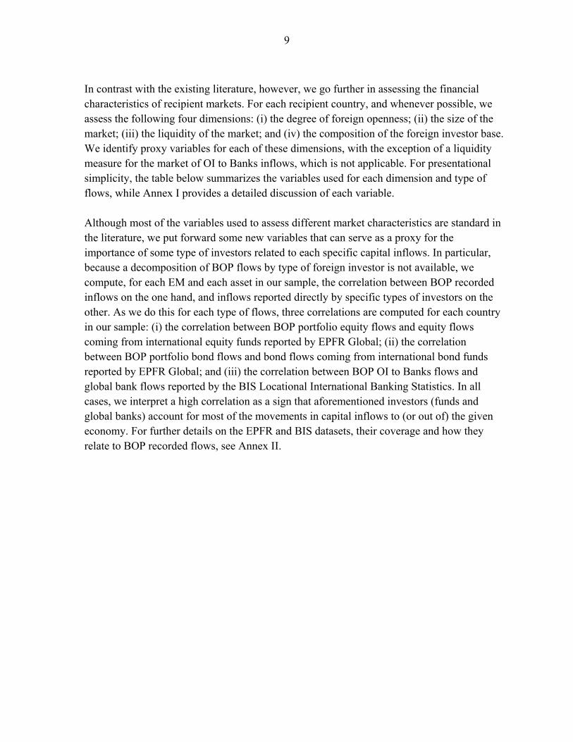
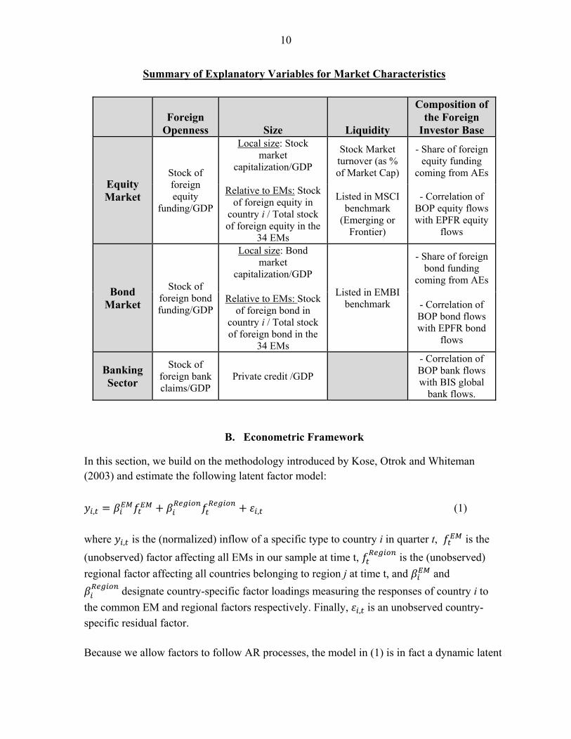
In contrast with the existing literature, however, we go further in assessing the financial characteristics of recipient markets. For each recipient country, and whenever possible, we assess the following four dimensions: (i) the degree of foreign openness; (ii) the size of the market; (iii) the liquidity of the market; and (iv) the composition of the foreign investor base. We identify proxy variables for each of these dimensions, with the exception of a liquidity measure for the market of OI to Banks inflows, which is not applicable. For presentational simplicity, the table below summarizes the variables used for each dimension and type of flows, while Annex I provides a detailed discussion of each variable. Although most of the variables used to assess different market characteristics are standard in the literature, we put forward some new variables that can serve as a proxy for the importance of some type of investors related to each specific capital inflows. In particular, because a decomposition of BOP flows by type of foreign investor is not available, we compute, for each EM and each asset in our sample, the correlation between BOP recorded inflows on the one hand, and inflows reported directly by specific types of investors on the other. As we do this for each type of flows, three correlations are computed for each country in our sample: (i) the correlation between BOP portfolio equity flows and equity flows coming from international equity funds reported by EPFR Global; (ii) the correlation between BOP portfolio bond flows and bond flows coming from international bond funds reported by EPFR Global; and (iii) the correlation between BOP OI to Banks flows and global bank flows reported by the BIS Locational International Banking Statistics. In all cases, we interpret a high correlation as a sign that aforementioned investors (funds and global banks) account for most of the movements in capital inflows to (or out of) the given economy. For further details on the EPFR and BIS datasets, their coverage and how they relate to BOP recorded flows, see Annex II.

10

Summary of Explanatory Variables for Market Characteristics

Foreign

Openness Size Liquidity

Composition of the Foreign

Investor Base

Equity Market

Stock of foreign equity

funding/GDP

Local size: Stock market

capitalization/GDP

Stock Market turnover (as % of Market Cap)

- Share of foreign equity funding

coming from AEs

Relative to EMs: Stock of foreign equity in

country i / Total stock of foreign equity in the

34 EMs

Listed in MSCI benchmark

(Emerging or Frontier)

- Correlation of BOP equity flows with EPFR equity

flows

Bond Market

Stock of foreign bond funding/GDP

Local size: Bond market

capitalization/GDP

Listed in EMBI benchmark

- Share of foreign bond funding

coming from AEs

Relative to EMs: Stock of foreign bond in

country i / Total stock of foreign bond in the

34 EMs

- Correlation of BOP bond flows with EPFR bond

flows

Banking Sector

Stock of foreign bank claims/GDP

Private credit /GDP

- Correlation of BOP bank flows with BIS global

bank flows.

B. Econometric Framework

In this section, we build on the methodology introduced by Kose, Otrok and Whiteman (2003) and estimate the following latent factor model:

, , (1)

where , is the (normalized) inflow of a specific type to country i in quarter t, is the

(unobserved) factor affecting all EMs in our sample at time t, is the (unobserved)

regional factor affecting all countries belonging to region j at time t, and and

designate country-specific factor loadings measuring the responses of country i to

the common EM and regional factors respectively. Finally, , is an unobserved country-

specific residual factor. Because we allow factors to follow AR processes, the model in (1) is in fact a dynamic latent

11

factor model. More precisely, we assume that idiosyncratic factors follow an AR(p) process:

, , , , , ⋯ , , , (2)

where , ~ 0, and , , , 0 for 0 and the world and regional factors

follow the respective AR(q) processes:

⋯ (3)

, , , ⋯ , , (4)

where ~ 0, , , ~ 0, and , , , , 0 for 0.

Given that the factors are unobservable, standard regression methods do not allow for the estimation of the model. As a consequence, we rely on Bayesian techniques as in Kose, Otrok and Whiteman (2003) for the estimation. As is standard in the literature, as a first step, we normalize the sign of the factor/loadings by (i) restricting the loading on the world factor for the first country in our sample to be positive and (ii) restricting the loadings on the regional factor for one country in each region to be positive. Second, to normalize the scales, we assume that each of the factor variances is equal to 1. Note that these normalizations do not affect the qualitative results and simply allow the identification of the model. In addition, we use Bayesian techniques with data augmentation to estimate the parameters and factors in (1)-(4). This implies simulating draws from complete posterior distribution for the model parameters and factors and successively drawing from a series of conditional distributions using a Markov Chain Monte Carlo (MCMC) procedure. Posterior distribution properties for the model parameters and factors are based on 300,000 MCMC replications after 30,000 burn-in replications. Following Kose, Otrok and Whiteman (2003), we use the following conjugate priors when estimating the model:

, ~ 0, (5)

, , … , , ~ 0, 1,0.5, … , 0.5 (6)

, … , ~ 0, 1,0.5, … , 0.5 (7)

, , … , , ~ 0, 1,0.5, … , 0.5 (8)

~ 6,0.001 (9) Where i=1,…, 34 and IG denotes the Inverse Gamma distribution, implying a rather diffuse

12

prior on the innovations variance. We also assume that the AR processes in (2)-(4) are stationary. In practice, in our implementation, we set the length of both the idiosyncratic and factor auto-regressive polynomials to 2. However, other (non-zero) values for p and q were tried with no substantial differences in the results. Similarly, reasonable deviations in priors did not generate any notable differences in the results presented below. Beside estimating the factors, we are particularly interested in measuring the influence of the common EM factor on the different EMs in our sample. As a result, most of the analysis below will focus on explaining the cross-country heterogeneity we observe in (i) factor

loadings and (ii) variance decomposition , where denotes the share of variance in country i’s funding that is attributable to the common EM dynamic. It is computed as follows:

/ , (10)

Intuitively, the loadings measure the contemporaneous impact of a sudden change in the direction of common EM factors on country i, whereas the variance decomposition is an estimate of the share of the total variance of country i’s funding that can be attributed to the common EM dynamics over the sample period. Finally, models are estimated using four regions, namely: (i) Latin America (ii) Asia (iii) Emerging Europe and (iv) Other. Table I provides the composition of each region. Note that although alternative regional decompositions could be used, the key results derived below are not sensitive to these decompositions as we focus on EMs’ sensitivity to the common

dynamics, captured through the or , both of which are invariant to the regional classification.

III. RESULTS

This section first presents the results of the factor estimation and discusses the cross sectional

dispersion we observe in the key statistics - and - highlighted above. After relating estimated factors to typical “observed” variables emphasized in the literature, we turn to a discussion of the country characteristics found to help explain the sensitivities of countries to global factors.

A. Factor Estimations, Factor Loadings and Variance Decompositions

The factor decomposition outlined in (1) yields the following three results. First, the model identifies precisely the commonality in (total) aggregated gross capital inflows to all EMs. Second, it shows that using total inflows conceals significant heterogeneity across assets.

13

While Portfolio Equity flows, Portfolio Bond flows and OI Banks do co-move across EMs, FDI and OI Non-Banks do not (Figure 2). Actually, with the exception of periods of global instability during which all flows go in the same direction, inflow dynamics can vary greatly across types of asset. This suggests, in turn, that different assets do not respond to the same driving (push or pull) forces, an aspect we analyze further in the next section. Third, the quantitative impact of the common EM dynamics varies a lot across markets and types of flows.

To show the heterogeneity in country responses, Figure 3 reports the coefficients estimated for equity, bond, and bank flows. In the case of equity flows, we find that a unit standard deviation in the common EM factor will generate, on impact, a unit standard deviation in equity flows to Pakistan and a 0.6 standard deviation in equity flows to India. In contrast, countries like Latvia, Estonia or Belarus do not experience any significant change in their foreign equity funding. Similarly, although Indonesia and South Africa bond flows react strongly to the common EM factor, bond flows to China, Colombia or Bulgaria are almost insensitive to the common dynamics.

Because the variance decompositions are a function of , the strong heterogeneity we observe in factor loadings naturally carries over to the variance decompositions. Table 4 reports the share of variance accounted for by the common EM factor and computed using equation (10). Intuitively, this variance decomposition provides a measure of the importance of this factor in driving the external funding of each country over the sample period. Note that because the model was not able to identify precisely any co-movement structure in the FDI and OI-to Non-Bank flows to EMs, only the results for Portfolio equity and bond flows and OI to bank flows, as well as aggregate inflows, are reported. Table 4 and Figure 3 highlight two important results. First, the impact of the common EM factors is large for a small number of countries – in particular for Asian countries - in the case of equity flows, whereas it is more evenly distributed across EMs for bond and bank flows. Second, substantial heterogeneity exists both across countries and across the different types of assets in the way common EM factors affect external funding. We can broadly identify three groups of EMs. The “high sensitivity” group contains countries that are relatively sensitive in all components, such as Brazil, Indonesia, Thailand, Turkey or South-Africa. The “asymmetric” group features countries with a high sensitivity in only one (or two) components, such as Pakistan, Philippines, India or Mexico. Finally, the “insensitive” group includes countries such as Estonia, Latvia or Chile that display very low relative sensitivity in all components. Interestingly, the highest sensitivities across all asset types are in this group. For instance, in the case of Pakistan and Philippines, more than half of the variance in their equity funding is accounted for by the common EM factor, implying that, to a great extent, both countries receive (or lose) equity funding whenever other EMs do.

14

B. What Drives the EM Common Dynamics?

In this section, we investigate the role of potential push and pull (internal) factors in driving the EM common factors estimated for the aggregate and each type of inflows in the previous section. In this context, we estimate the following equations for the EM common factors on aggregated inflows and separately for Portfolio Bond, Portfolio Equity, OI to Banks: (11) where the vectors include the general push, pull and type specific variables presented in Section 2. Given the 2001Q2-2013Q4 coverage of our sample, the total number of observations is 50. The signs of the coefficients of push variables are expected to be negative. A slowdown in growth in advanced economies leads to an expansion of capital flows to emerging market economies, as investors take advantage of better growth opportunities and higher yields (e.g., Reinhart and Reinhart, 2008). An increase in the VIX, i.e., increased uncertainty, is usually associated with a decrease of cross-border flows, as per Rey (2013). Similarly, an increase in the U.S. REER likely reduces cross-border flows since borrowers become riskier and less solvent in U.S. dollar terms as their currencies depreciate, as noted in Bruno and Shin (2015). A flatter yield curve, reflecting less profitable investment opportunities at home, may also trigger a search for yield abroad. For example, banks, which borrow short-term and lend long term, might turn to cross-border investments when the yield curves flattens, as also found by Cerutti, Claessens and Ratnovski (2014). Finally, higher expected policy rates would reduce cross-border flows to EMs since the opportunity and funding costs are expected to increase for investors. Most of the pre-crisis literature has used the level of a short term rate, such as the U.S. policy rate, but, following more recent analysis (e.g., Koepke 2014), we use the change in expected U.S. policy rates, also to deal with fact that the policy rate has been very stable in recent years. The expected sign of coefficients attached to commodity prices and to growth in EM economies are both positive. Since many EMs are net exporters of commodities, higher commodity prices, improve EMs’ economic perspectives and thus likely boost cross-border flows.9 With regard to the type (or asset) specific factors, the coefficients for return chasing variables and bank leverage are all expected to be positive since a high leverage indicates a lower perceived risk and higher willingness and capacity of banks to lend (Adrian and Shin, 2014; Bruno and Shin, 2015a). 9 Reinhart and Reinhart (2008) found evidence of a statistically significant and positive relationship between commodity prices and capital inflows between 1967 and 2006.

EMt t t t tf Push Pull Type Specific Factors

15

The actual regression results (Table 5) indicate that almost all coefficients, when statistically significant, have the expected signs. Among the push variables, VIX and REER are the most robust factors behind the commonality in aggregate inflows as well as in the various types of capital inflows (see columns 1, 5, 9, and 13). In contrast, the slope of the yield curve, GDP growth rate of core countries or the expected policy are only significant in some cases. 10 The explanatory power of the VIX is, however, very much driven by the global financial crisis, as shown in Figure 4. When using pull factors only, we find the price of commodities to be the only significant variable across the various types of capital inflows, with EM growth only significant in the case of OI to bank and total inflows (see columns 2, 6, 10 and 14). When push and pull variables are used simultaneously, the same results are found (see columns 3, 7, 11 and 15).11 In terms of explanatory power, we find that push factors dominate pull factors, even when asset-specific variables are included in the regressions (see columns 4, 8, 12, and 16), even though the latter themselves are also statistically significant and with the expected sign. As reported in the group level R2s, push factors account for about 65 percent of the overall R2s in the case of OI banks, about 60 percent of the R2s for Portfolio bonds, and about 75 percent in the case of Portfolio equity flows. In sum, the analysis of the drivers of the EM common dynamic clearly indicate that, as expected, various global push variables play a major role, but with the relative importance of some factors varying across types of flows.

C. What Drives the Impact of Global Push Factors Across Countries?

Next, we investigate what makes a country more sensitive (or immune) to changes in push factors. Why do some countries always gain (or lose) more inflows relative to other countries when conditions in core countries change? We take an agnostic approach and investigate whether macroeconomic and institutional fundamentals or financial market characteristics might explain such heterogeneity. In practice, this means that we regress the estimated factor

loadings for each asset (separately) on our two sets of fundamental-related and market-structure based variables introduce in Section 2 (see further Annexes I and II for a thorough discussion of the variables). Formally, the following cross-sectional regression is estimated for each type of flow separately:

. . (12)

10 The significant coefficient on G4 GDP growth on the bank regression is opposite to the expected one, but it could be capturing the fact that higher growth rates in core economies often tend to increase global bank funding (e.g. more deposits, etc), which could trigger positive cross-border flows 11 The only exception is EM GDP growth, which seems to lose explanatory power and even flip signs when used with more variables. It is excluded in some regressions for this motive.

16

Before turning to our key findings, we acknowledge that our benchmark regressions results are subject to some limitations. By construction, estimations are based on a small sample of 34 cross-country observations (for each asset). Given the sample size, using all (14) fundamental-related and market-structure based variables at once is therefore practically infeasible. To overcome these constraints, we use the following strategy: we first regress the

on the fundamentals and market variables separately. We then combine the variables that are significant in each category (if any) in one regression. To confirm that this procedure yields stable results, a Bayesian Model Averaging exercise is performed in the next section. At this point however, we emphasize that all results presented below are very robust to the issue of model uncertainty. Table 6 provides the benchmark results, which are as follows. First, for the case of equity and bank flows, higher betas do not coincide with “weaker” fundamentals such as lower growth, higher debt level or poor institutions (columns 1-3 and 7-9).12 As far as bond flows are concerned (columns 4-6), we find that countries with a higher level of reserves, higher trade openness and a more flexible foreign exchange regime are more sensitive to global push factors. Second, we find that our proxies for the importance of global investors (international mutual funds in the case of equity and bond flows, and global banks in the case of OI-to-bank flows) are highly significant and suggest a potentially strong quantitative impact for all types of assets. For instance, we find that going from a zero to a perfect correlation increases the predicted response to a shock in the common EM factor by 0.45 for equity, 0.24 for bonds and 0.75 for banks. Given the general levels of the betas, as also depicted in Figure 3, these are large effects. Third, equity markets that are more liquid (as measured by the turnover ratio) and belong to the MSCI Frontier index have a higher beta. Altogether, we also find that most of the cross sectional variation in loadings can be explained by the market-related variables. To sum up, the results show that EMs’ sensitivity to the common dynamics varies across countries and type of flows; with the nature of the investor base having the more important role in explaining the cross-country differences in the case of equity and bank flows, and also, although to a lesser extent, in the case of bond flows. Macroeconomic fundamentals (e.g., level of reserves, trade openness, and the type of exchange rate regimes) seem to be playing a key role in the case of bond flows. However there is no robust evidence that “good” macroeconomic (e.g., public debt, growth) or institutional fundamentals (e.g., Investment Climate and Rule of Law) have a role in explaining EM different sensitivities to global push factors.

12 Only bank flows seems to be sensitive to the choice of the exchange rate in column 7, but this result disappear once we control by market structure variables (column 9).

17

D. Robustness

This section provides some robustness checks. We first show that the estimated betas used in the regression are not only a reflection of the Great Financial Crisis (GFC), but that they also reflect outcomes during other periods of sharp variations in global push factors. When comparing factor loadings with actual retrenchments in capital flows during the GFC and the Taper Tantrum, we find that, in the overwhelming majority, countries with higher betas suffered a deeper retrenchment in flows in both episodes. This positive relationship is illustrated in Figure 5, which plots the beta coefficients for each asset on the y axis against the actual loss in funding experienced during the GFC (left panel) and the Tantrum (right panel). This finding shows that our approach is indeed capturing the “actual” sensitivity of most EM countries during periods of sharp movements in global push factors. Second, we show that the variables shown to be significant in the benchmark regression analysis are very robust to changes in covariates. Given the limited cross section at our disposal and the larger number of explanatory variables, the simple strategy we used to identify robust correlates might lead to misleading results. To address this issue of model uncertainty, we use a Bayesian Model Averaging (BMA) for each regression.13 In practice, BMA methods run the maximum combination of models and provide estimates and inference results that take into account the performance of the variable not only in the final “reported” model but over the whole set of possible specifications. After performing this robustness test, we find that the significant variables in the base regressions are always the most robust variables in the Bayesian averaging exercise (Table 7). Third, we find that institutional fundamentals are not themselves driving the importance of global investors (fund or bank) in our sample. In particular, one could expect that countries with strong institutional fundamentals attract more global investors to begin with. As a result, the correlation variables that we found to be significant could be indirectly proxying for the quality of local institutions. However, we do not find any relation between the correlations used in the previous sections and the institutional quality of recipient markets, as measured by the value of Law and Order and Investor Protection Index computed by ICRG (Figure 6).

IV. CONCLUSION AND POLICY IMPLICATIONS

After analyzing the sensitivity of 34 EMs to global push factors, we find that the cross-country differences in EM sensitivities to global push factors are, to a great extent, a function of market characteristics. In particular, the nature of a country’s foreign investor base (the

13 From a technical point of view, the BMA technique used here follows Fernandez, Ley, and Steel (2001).

18

larger the role of international mutual funds in the case of equity and bond flows, and global banks in the case of bank inflows) explains the higher sensitivity of some EMs to global push factors. Macroeconomic fundamentals, in particular the type of FX regime, seem to be playing a key role in explaining cross-country sensitivities; but only in the case of bond flows. Last, but not least, we do not find evidence that institutional fundamentals (e.g., Investor Protection, Rule of Law) or standard measures of macroeconomic performance (higher growth, lower debt) have a role in explaining EM different sensitivities to global push factors. Although these results have potentially important implications for EMs, they require a careful interpretation. First, we emphasize that our findings do not mean that borrowers’ fundamentals do not matter in shaping other crucial properties of capital flows to EMs. As a number of contributions have convincingly shown (e.g., Alfaro et al 2008), countries with macroeconomic or institutional deficiencies tend to receive less capital inflows, a result we confirm in our EM sample. Different from this “level” effect, however, our findings suggests that the traditional “push factor” debate may have over-stated the importance of fundamentals in shaping sensitivities to external shocks at the expense of other important determinants. In other words, good fundamentals do not assure a country’s insulation from global financial shocks. From a policy perspective, this implies that authorities in EMs should put efforts into collecting information about their foreign investor base and the role of large funds (or asset management companies) in it. While systematic and reliable information on the decomposition of foreign holdings by type of investors is still insufficient, despite recent efforts (see for instance Arslanalp and Tsuda, 2014), our analysis already shows that some measures can be created and used to assess countries’ sensitivities. Finally, we emphasize that further research is needed to understand the final macroeconomic impact of push factors at the country level. Although some countries might be highly sensitive to push factors, a number of parameters could dampen the overall impact of such waves of positive (or negative) inflows. For instance, the presence of a large pool of domestic investors absorbing the assets from foreigners leaving the country in times of stress could mitigate the final price and overall financial and economic impacts of sudden pressure in flows. A notable example among EMs in this respect is Malaysia, which is found to be sensitive to push factors in all assets in our analysis, but where negative inflows in times of stress are usually offset by local institutional investors repatriating foreign assets (IMF, 2013b). Examining discrepancies between how flows and asset prices react to global push factors, and this connects to the local institutional set up, constitutes useful avenues that we leave for further research.

19

References Alfaro, Laura, Sebnem Kalemli-Ozcan, and Vadim Volosovych, 2008, “Why Doesn't Capital

Flow from Rich to Poor Countries? An Empirical Investigation,” Review of Economics and Statistics, Vol. 90, No. 2, pp. 347-68.

Adrian, Tobias, and Hyun Song Shin, 2010, “Liquidity and Leverage,” Journal of Financial Intermediation, Vol. 19, No. 3, pp. 418-37.

–––––, 2014, “Procyclical Leverage and Value-at-Risk,” Review of Financial Studies, Vol. 27 No. 2, pp. 373-403.

Aizenman, Joshua, Mahir Binici, and Michael M. Hutchison, 2014, "The Transmission of Federal Reserve Tapering News to Emerging Financial Markets," NBER Working Paper No. 19980.

Ahmed Shaghil, Coulibaly Brahima, Zlate Andrei, 2014, “International Financial Spillovers

to Emerging Market Economies: How Important Are Economic Fundamentals?” Board of Governors of the Federal Reserve System Working Paper D2015-37.

Arslanalp, Serkan, and Tsuda, Takahiro, 2014, “Tracking Global Demand for Advanced

Economy Sovereign Debt. IMF Economic Review, Vol. 62, Issue 3, pp. 430-64. Broner, Fernando, Tatiana Didier, Aitor Erce, and Sergio L. Schmukler, 2013, “Gross Capital

Flows: Dynamics and Crises,” Journal of Monetary Economics Vol. 60, No. 1, pp. 113-33.

Bruno, V., and Hyun Song Shin, 2015a, “Cross-Border Banking and Global Liquidity,”

Review of Economic Studies, forthcoming.

Bruno, V., and Hyun Song Shin, 2015b, “Capital Flows and the Risk-Taking Channel of Monetary Policy,” Journal of Monetary Economics, forthcoming.

Calvo, Guillermo, Leonardo Leiderman, and Carmen Reinhart, 1993, “Capital Inflows and Real Exchange Rate Appreciation in Latin America: The Role of External Factors,” IMF Staff Papers, Vol. 40, No. 1, pp. 108-51.

Calvo, Guillermo, Leonardo Leiderman, and Carmen Reinhart, 1996, “Inflows of Capital to Developing Countries in the 1990s,” Journal of Economic Perspectives, Vol. 10, No. 2, pp.123-39.

Cerutti, Eugenio, and Stijn Claessens, 2014, “The Great Cross-Border Bank Deleveraging: Supply Side Characteristics and Intra-Group Frictions,” IMF Working Paper 2014/180.

Cerutti, Eugenio, Stijn Claessens, and Patrick McGuire, 2012, "Systemic Risks in Global Banking: What Available Data Can Tell Us and What More Data are Needed?" NBER Working Papers 18531, NBER.

20

Cerutti, Eugenio, Stijn Claessens, and Lev Ratnovski, 2014, “Global Liquidity and Drivers of Cross-Border Bank Flows,” IMF Working Paper, 2014/69.

Cetorelli, Nicola, and Linda Goldberg, 2012a, “Liquidity Management of U.S. Global Banks: Internal Capital Markets in the Great Recession,” Journal of International Economics, Vol. 88, pp. 299-311.

–––––, 2012b, “Banking Globalization and Monetary Transmission,” Journal of

Finance, Vol. 67, No. 5, pp. 1811-843. Chuhan, Punam, Stijn Claessens, and Nlandu Mamingi, 1998, “Equity and Bond Flows to

Asia and Latin America: The Role of Global and Country Factors,” Journal of Development Economics, Vol. 55, pp. 439-63.

Claessens, Stijn, and Swati Ghosh, 2013, “Capital Flow Volatility and Systemic Risk in Emerging Markets: The Policy Toolkit,” in O. Canuto and S. Ghosh (eds.), Dealing with Challenges of Macro Financial Linkages in Emerging Markets, World Bank, Washington, D.C.

Claessens, Stijn, and Neeltje Van Horen, 2014, “Foreign Banks: Trends and Impact,” Journal

of Money, Credit, and Banking, Vol. 46, No. 1, pp. 295-326. Eichengreen, Barry, and Poonam Gupta, 2014, "Tapering Talk: The Impact of Expectations

of Reduced Federal Reserve Security Purchases on Emerging Markets," Policy Research Working Paper Series 6754, The World Bank.

Fernandez, Carmen, Eduardo Ley, and Mark Steel, 2001, “Benchmark Priors for Bayesian

Model Averaging,” Journal of Econometrics, Vol. 100, No. 2, pp. 381-427. Forbes, Kristin J., and Francis E. Warnock, 2012, “Debt- and Equity-Led Capital Flow

Episodes,” NBER Working paper, No. 18329. Forbes, Kristin J., 2007. "The Microeconomic Evidence on Capital Controls: No Free

Lunch," in Capital Controls and Capital Flows in Emerging Economies: Policies, Practices and Consequences, pp. 171-202, NBER.

Fratzscher, Marcel, 2011, “Capital flows, Push versus pull factors and the global financial

crisis,” ECB Working Paper No 1364.

Fratzscher, Marcel, Marco Lo Duca, and Roland Straub, 2013, “On the International Spillovers of U.S. Quantitative Easing,” Discussion Papers of DIW Berlin 1304, DIW Berlin, German Institute for Economic Research.

Ghosh, Atish R., Mahvash Qureshi, Jun Il Kim, and Juan Zalduendo, 2014, "Surges,"

Journal of International Economics, Vol. 92, No. 2, pp. 266-85. IMF, 2013a, “Global Impact and Challenges of Unconventional Monetary Policies,

Background paper,” Washington, D.C.: IMF.

21

IMF, 2013b, "The Yin and Yang of Capital Flow Management: Balancing Capital Inflows with Capital Outflows," by Jaromir Benes, Jaime Guajardo, Damiano Sandri, and John Simon, World Economic Outlook, Chapter 4, Fall.

Jotikasthira, Chotibhak, Christian Lundblad, and Tarun Ramadorai, 2012, “Asset Fire Sales

and Purchases and the International Transmission of Funding Shocks,” Journal of Finance, Vol. 67, No. 6, pp. 2015–050.

Koepke, Robin, 2014, “Fed Policy Expectations and Portfolio Flows to Emerging Markets,” IIF Working Paper, May, Washington, D.C..

Koepke, Robin, 2015, “What Drives Capital Flows to Emerging Markets: A Survey of the Empirical Literature,” IIF Working Paper, April, Washington D.C..

Koepke, Robin, and Saacha Mohammed, 2014, “Portfolio Flows Tracker FAQ,” IIF Research Note.

Kose, Ayhan, Christopher Otrok, and Charles H. Whiteman, 2003, “International Business Cycles: World, Region, and Country-Specific Factors,” American Economic Review, Vol. 93, No. 4, pp. 1216-239.

Magnus, Jan, Powell,O and Prufer, P, 2010, “A Comparison of Two Model Averaging Techniques with an Application to Growth Empirics.” Journal of Econometrics, Vol. 154, No. 2, pp. 139-153.

Minoiu, Camelia, and Javier Reyes, 2013, “A Network Analysis of Global Banking: 1978-2010,” Journal of Financial Stability, Vol. 9, No. 2, pp. 168-84.

Milesi-Ferretti, Gian Maria, and Cédric Tille, 2011, "The Great Retrenchment: International Capital Flows during the Global Financial Crisis," Economic Policy, Vol. 26. No. 66, pp. 285-342.

Prachi, Mishra, Kenji Moriyama, Papa N'Diaye, and Lam Nguyen, 2014, "Impact of Fed Tapering Announcements on Emerging Markets," International Monetary Fund and the Reserve Bank of India. Mimeo.

Puy, Damien, 2013, "Institutional Investors Flows and the Geography of Contagion," Economics Working Papers ECO2013/06, European University Institute.

Raddatz, Claudio, and Sergio Schmukler, L., 2012, "On the International Transmission of Shocks: Micro-evidence from Mutual Fund Portfolios," Journal of International Economics, Vol. 88, No. 2, pp. 357-74.

Rey, Hélène, 2013, “Dilemma not Trilemma: The Global Financial Cycle and Monetary Policy Independence,” in Proceedings of the Federal Reserve Bank of Kansas City Economic Symposium at Jackson Hole.

Sahay, Ratna, Vivek Arora, Thanos Arvanitis, Hamid Faruqee, Papa N'Diaye, Tommaso Mancini-Griffoli, and an IMF Team, 2014. “Emerging Market Volatility: Lessons from the Taper Tantrum,” IMF Staff Discussion Note SDN 14/09, September.

Shin, Hyun Song, 2012, “Global Banking Glut and Loan Risk Premium” Mundell‐Fleming Lecture, IMF Economic Review Vol. 60, No. 2, pp. 155‐92.

22

Table 1. Sample of Countries

Latin America Asia Emerging Europe Other

Argentina India Belarus Turkey

Brazil China, Mainland Kazakhstan South Africa

Chile Indonesia Bulgaria Israel

Colombia Republic of Korea Russian Federation

Mexico Malaysia Ukraine

Peru Pakistan Czech Republic

Uruguay Philippines Slovak Republic

Venezuela, Rep. Bol. Thailand Estonia

Latvia

Hungary

Lithuania

Croatia

Slovenia

Poland

Romania

23

Table 2. Variable Definitions, Frequency and Sources

Variable Definition Frequency Source

Capital Flows

Capital inflows

gross inflow as % GDP, total and by component

Quarterly IMF Balance of Payment Statistics

Global Bank flows inflow as % GDP Quarterly

Bank of International Settlements - Locational Statistics

Mutual Fund Flows inflow as % GDP Quarterly EPFR

Push/Pull factor Analysis

Real GDP Growth

in %, QoQ, un-weighted average of US, Euro Area, Japan, and UK

Quarterly IMF WEO

US VIX CBOE S&P500 Volatility VIX Quarterly Datastream

Expected Change in Policy Rate

Difference between Policy Rate and 30 Day Federal Funds 6 Month Futures

Quarterly, average of monthly figures

Datatream and Cleveland Fed

US Yield Curve 10 year/3 month US Treasury yield spread Quarterly Datastream

US REER US Real Effective Exchange Rate Quarterly IMF WEO

Commodity Prices growth rate, QoQ Quarterly IMF WEO

US Dealer Bank Leverage (Equity+Total Liabilities)/Equity Quarterly US Fund Flows

US TED Spread 3-month TED spread (LIBOR - Treasury bill) Quarterly Datastream

10Y Bond Yield 10 year US Tresuary yield Quarterly Datastream

MSCI returns Return in the MSCI EM index Quarterly Datastream

EMBI returns Return in EMBI index Quarterly Datastream

Macroeconomic and Institutional fundamentals

Trade Openness (X+M)/GDP

Average over 2001-2013

World Development Indicators

FX regime* Index from 1 to 13


Ilzetzki, Reinhart and Rogoff (2004)

Public Debt as % GDP



Reserves as % GDP



Real GDP Growth %, annual



Rule of Law* Index from 1 to 10


ICRG

Investor Protection* Index from 1 to 10


ICRG

Cont’d…

24

Table 2. Variable Definitions, Frequency and Sources...contd…

Variable Definition Frequency Source

Market Characteristics

Foreign Openness

Stock of foreign Equity, Bond or Bank claims/GDP


IIP

Stock Market Capitalization

Stock Market Cap/GDP Average over 2001-2013

World Bank Financial Development Database

Bond Market Capitalization**

Bond Market Cap/GDP Average over 2001-2013


Private Credit Bank Credit to the Private Sector/GDP



Stock Market Turnover

Sum of all shares traded over the period / Stock market cap.



Share of Funding coming from Advanced Economies

Sum of Bond (Equity) coming from AEs and Financial centers***/Total Bond (Equity) Funding


CPIS

MSCI EM

Country listed in the MSCI Emerging index over the sample period

Dummy Morgan Stanley

MSCI FM

Country listed in the MSCI Frontier Market index over the sample period

Dummy Morgan Stanley

EMBI EM Country listed in the EMBI Emerging index over the sample period

Dummy JP Morgan

* In the case of ICRG ratings, a higher value of the index indicates better institutions. For the FX regime, a higher value implies a more flexible exchange rate. ** Bond Market Capitalization data are not available for all countries in our sample. When used on the restricted sample however, the bond market capitalization is not found significant. *** See Annex I for the list of source countries.

25

Table 3. Raw Statistics

Variables Obs Mean Std. Dev. Min Max

Fundamentals

Trade Openness 34 80.52 41.22 23.99 187.30

Public debt 34 40.69 19.08 5.95 79.21

Reserves 34 19.58 9.37 6.96 44.33

Exchange Rate Regime 34 8.29 3.04 2.00 13.00

Average Growth 34 4.76 1.73 0.78 9.94

Investor Protection 34 8.83 1.73 3.69 11.23

Rule of Law 34 3.59 1.01 1.54 5.00

Equity Market Characteristics

Foreign Openness -Equity 34 6.88 7.01 0.07 24.59

Relative Market Size -Equity 34 2.94 4.66 0.00 17.36

Stock Market Capitalization 33 43.19 40.52 0.49 190.54

MSCI EM Country 34 0.59 0.50 0.00 1.00

MSCI FM Country 34 0.29 0.46 0.00 1.00

Stock Market turnover 33 49.59 59.50 0.96 226.99

Share of Equity Funding from Advanced Economies 34 67.19 22.72 12.48 95.67

BOP Equity correlation with EPFR flows 34 0.24 0.26 -0.41 0.73

Bond Market Characteristics

Foreign Openness -Bond 34 10.04 6.48 0.12 30.47

Relative Market Size - Bond 34 2.94 4.22 0.00 19.27

EMBI Country 34 0.65 0.49 0.00 1.00

Share of Bond funding from Advanced Economies 34 67.27 16.74 23.25 92.09

BOP Bond correlation with EPFR flows 34 0.26 0.26 -0.55 0.67

Banking Market Characteristics

Foreign Openness - Other Investment 34 36.29 19.08 4.32 96.40

Private Credit/GDP 32 63.39 29.11 24.57 138.60

BOP OI-Bank correlation with BIS flows 34 0.13 0.22 -0.52 0.59

26

Table 4. Variance Decompositions Results This table reports, for each country in our sample, the (mean) of the share of variance accounted for by common and regional factors, as presented in Section 2. Results for aggregated inflows are reported under the column “All inflows”. Results by type of flows are reported under the corresponding column.

Portfolio Equity Portfolio Bond OI Bank All inflows

Global Regional Global Regional Global Regional Global Regional

Latin America

Argentina 25% 7% 12% 11% 29% 5% 12% 20%

Brazil 24% 4% 25% 6% 25% 11% 27% 5%

Chile 2% 10% 2% 20% 4% 4% 11% 13%

Colombia 1% 12% 1% 20% 8% 6% 1% 32%

Mexico 7% 8% 29% 11% 8% 32% 20% 15%

Peru 3% 5% 8% 2% 26% 3% 34% 19%

Uruguay 2% 16% 18% 14% 0% 8% 1% 3%

Venezuela, Rep. Bol. 0% 6% 7% 6% 3% 11% 3% 16%

Average 8% 8% 13% 11% 13% 10% 14% 15%

Asia

India 35% 16% 4% 34% 7% 2% 55% 4%

China,P.R.: Mainland 18% 4% 2% 3% 35% 7% 28% 1%

Indonesia 18% 8% 43% 9% 23% 23% 21% 8%

Korea, Republic of 7% 12% 11% 2% 19% 38% 50% 12%

Malaysia 18% 4% 16% 6% 22% 38% 39% 45%

Pakistan 60% 18% 13% 7% 1% 2% 2% 10%

Philippines 48% 4% 11% 2% 6% 2% 26% 1%

Thailand 32% 15% 17% 21% 20% 7% 53% 13%

Average 29% 10% 15% 11% 16% 15% 34% 12%

Emerging Europe

Belarus 0% 0% 10% 16% 7% 0% 1% 3%

Kazakhstan 30% 2% 20% 11% 1% 42% 4% 34%

Bulgaria 16% 62% 1% 2% 5% 38% 6% 60%

Russian Federation 8% 2% 15% 3% 23% 37% 36% 17%

Ukraine 3% 0% 11% 2% 10% 68% 8% 36%

Czech Republic 1% 10% 17% 10% 21% 6% 1% 12%

Slovak Republic 1% 1% 16% 3% 5% 9% 0% 2%

Estonia 1% 91% 5% 2% 1% 53% 6% 39%

Latvia 1% 1% 5% 46% 4% 59% 11% 50%

Hungary 1% 0% 14% 3% 1% 25% 1% 35%

27

Table 4. Variance Decompositions Results…contd…..

Lithuania 1% 16% 12% 5% 1% 75% 5% 63%

Croatia 3% 0% 1% 5% 15% 2% 2% 36%

Slovenia 35% 1% 4% 2% 5% 64% 17% 40%

Poland 1% 3% 22% 9% 1% 24% 32% 11%

Romania 30% 1% 11% 10% 2% 60% 8% 69%

Average 9% 13% 11% 9% 7% 38% 10% 43%

Other

Turkey 22% 20% 26% 3% 37% 6% 36% 5%

South Africa 17% 14% 30% 22% 22% 10% 41% 18%

Israel 3% 33% 13% 39% 2% 53% 17% 30%

Average 14% 22% 23% 10% 20% 23% 24% 29%

Table 5. Finding the Drivers of the Estimated EM Common Factors

This table reports the results of the regressions of the EM common factors (Portfolio Bond, Portfolio Equity, OI to Banks, and total flows) on the set push, pull and type specific variables presented in Section 2, during the period 2001Q2-2013Q4, and as stated in Equation 11 in the main text. Definitions, sources and frequency of all variables are presented in Table 2. Columns (1), (5), (9) and (13) report the results when push variables are used as regressors. Columns (2), (5), (10) and (14) report results only when push variables are used. Columns (3), (7), (10) and (15) report results when both push and pull variables are used. Finally, columns (4), (8), (12) and (16) report results when also type specific variables are added to pull and push variables. Robust standard errors are in parentheses. Asterisks denote significant coefficients, with ***, **, * indicating significance at 1%, 5%, and 10% percent level, respectively. R-squared at the group level are calculated based on the Shapley decomposition.

VARIABLES bank bond equity total

[1] [2] [3] [4] [5] [6] [7] [8] [9] [10] [11] [12] [13] [14] [15] [16] Core_GDP_Growth 0.132*** 0.0736* 0.0547 -0.00808 -0.0416 -0.0308 0.0527 0.0588 0.0329 0.0789* 0.00857 -0.0351

(0.0387) (0.0412) (0.0426) (0.0543) (0.0583) (0.0627) (0.0535) (0.0526) (0.0532) (0.0418) (0.0388) (0.0417) US VIX -0.0313*** -0.0161 0.00183 -0.0516*** -0.0356*** -0.0353*** -0.0273*** -0.0218* -0.0232* -0.0397*** -0.0209** 0.00264

(0.0105) (0.0112) (0.0154) (0.00997) (0.0106) (0.0104) (0.00839) (0.0130) (0.0116) (0.0108) (0.00991) (0.0167) Exp. Change in Policy Rate -0.117 -0.101 -0.00785 -0.325 -0.194 -0.198 0.0101 0.126 -0.0690 -0.401* -0.372* -0.415*

(0.265) (0.232) (0.253) (0.289) (0.304) (0.289) (0.342) (0.370) (0.333) (0.235) (0.214) (0.206) US yield_curve -0.0110 -0.127 -0.0374 0.118 -0.1000 -0.0131 -0.258** -0.392** -0.268** -0.0820 -0.233** -0.164

(0.0702) (0.104) (0.107) (0.114) (0.167) (0.126) (0.110) (0.147) (0.108) (0.0849) (0.102) (0.132) US REER -0.0592*** -0.0567*** -0.0855*** -0.0386*** -0.0454*** -0.0172 0.00337 -0.00481 0.00386 -0.0358*** -0.0334*** -0.0617***

(0.00995) (0.0115) (0.0188) (0.00755) (0.00942) (0.0121) (0.00807) (0.00903) (0.00808) (0.00776) (0.00940) (0.0182) Commodityprice_pch 0.0561*** 0.0314** 0.0282** 0.0451*** 0.0241* 0.0291** 0.0222* 0.00262 -0.00673 0.0552*** 0.0382*** 0.0279**

(0.0119) (0.0119) (0.0124) (0.0121) (0.0129) (0.0133) (0.0129) (0.0153) (0.0156) (0.0131) (0.00954) (0.0119) L.RGDP_EM_growth 0.0988** -0.0396 -0.0399 0.00976 -0.120** 0.0530 -0.0896* 0.0896* -0.0551 -0.0153

(0.0439) (0.0551) (0.0600) (0.0530) (0.0530) (0.0508) (0.0530) (0.0448) (0.0417) (0.0445) Global_bank_leverage 0.0682** 0.0569

(0.0335) (0.0516) TED -0.527** -0.778**

(0.261) (0.292) US 10 bond yield -0.240* 0.0382

(0.135) (0.130) L.EMBI_growth 0.0330* -0.00357

(0.0165) (0.0139) L.MSCI_growth 0.0153** 0.0195

(0.00592) (0.0125) Observations 50 50 50 50 50 50 50 50 50 50 50 50 50 50 50 50 R-squared (overall) 0.660 0.415 0.710 0.731 0.510 0.238 0.569 0.580 0.396 0.091 0.421 0.436 0.643 0.468 0.733 0.789 R-squared (push variables) 0.660 - 0.477 0.477 0.510 - 0.420 0.330 0.396 - 0.363 0.327 0.643 - 0.454 0.381 R-squared (pull variables) - 0.415 0.233 0.234 - 0.238 0.149 0.144 - 0.091 0.058 0.026 - 0.468 0.279 0.227 R-squared (type variables) - - - 0.021 - - - 0.106 - - - 0.083 - - - 0.181

18

18 1828 28

Table 6. Explaining Countries’ Sensitivities to Push Factors

This table presents the results of the estimation of the regression of EM sensitivities in each type of flow on the set of macro, institutional and market characteristics presented in Section 2, Annex I and Annex 2. Definitions, sources and frequency of all variables is presented in Table 2. Columns (1), (4) and (7) report the results when only macroeconomic and institutional fundamentals are used as regressors. Columns (2), (5) and (8) report results only when market characteristics are used. Finally, columns (3), (6) and (9) report results when using as regressors the variables that are found significant in each sub-group. For a robustness check of this approach and corresponding results, see Section 4.

Equity Beta Bond Beta Bank Beta

(1) (2) (3) (4) (5) (6) (7) (8) (9)

Fundamentals

Trade Openness -0.000236 0.00179** 0.00110** 0.000708

Debt/GDP 0.00163 0.00193 -0.00104

Reserves/GDP 0.00190 -0.00450 -0.00559*** 0.00567

FX Regime 0.0192 0.0315*** 0.0203** 0.0342** 0.00766

Average Growth 0.0508 0.0122 0.0486

Investor Protection -0.0114 -0.00423 0.000348

Law and Order -0.0199 -0.0256 -0.0696

Market Characteristics

Foreign Openness 0.000124 0.00281 -0.00306

Local Market Size (%GDP) 0.000714 0.000733

Relative Market Size -0.00328 0.00608

MSCI EM Benchmark (dummy) -0.0648 0.0233

MSCI Frontier Benchmark (dummy) 0.228*** 0.242***

Turnover Ratio 0.00176*** 0.00170***

Share of Funding from AE 0.00167 0.00108

Correlation with EPFR (or BIS) flows 0.474*** 0.454*** 0.260** 0.241** 0.705*** 0.75***

constant 0.0123 -0.0369 0.0637 -0.0130 0.110 0.101 -0.207 0.146 0.0994

R-sq 0.244 0.546 0.521 0.409 0.288 0.429 0.324 0.520 0.530

29

Table 7. Bayesian Averaging Results Given our limited cross section, standard regression methods could fail to select robust relations. To address this issue and confirm the significance of the variables highlighted in section 3, we use a Bayesian Model Averaging technique presented in Fernandez, Ley, and Steel (2001). Intuitively, the objective of Model Averaging is to address the problem of model uncertainty by (i) running the maximum combination of models and (ii) providing estimates and inference results that take into account the performance of the variable not only in the final “reported” model but over the whole set of specifications. In practice, these two steps boil down to estimate a parameter of interest conditional on each model in the model space and computing the unconditional estimate as a weighted average of the conditional estimates. This table 6 reports the results of the Bayesian Averaging obtained for the Equity, Bond and Bank regressions presented in Section 3.c. Along with coefficient and t-statistics, it reports individual Post-Inclusion Probabilities (henceforth PIPs). In line with Magnus et al. (2010), variables with the highest PIPs are considered as robust. Overall, we find that our key results (i.e. those related to market characteristics) are very robust to the variation in the set of regressors.

Equity- Bayesian Averaging Bond- Bayesian Averaging Bank - Bayesian Averaging

Coef. t-Stat PIP Coef. t-Stat PIP Coef. t-Stat PIP

Trade/GDP 0.000 -0.17 0.09 Trade/GDP 0.000 0.3 0.15 Trade/GDP -0.041 -0.79 0.47

Debt/GDP 0.000 0.04 0.07 Debt/GDP 0.000 0.24 0.12 Debt/GDP -0.024 -0.4 0.21

Reserves/GDP 0.000 -0.02 0.07 Reserves/GDP -0.001 -0.41 0.21 Reserves/GDP 0.023 0.25 0.14

FX Regime 0.002 0.29 0.13 FX Regime 0.019 1.34 0.73 FX Regime 0.048 0.19 0.12

Average Growth 0.008 0.43 0.22 Average Growth -0.001 -0.14 0.1 Average Growth -0.017 -0.05 0.1

Investor Protection -0.003 -0.27 0.13 Investor Protection 0.000 -0.05 0.09 Investor Protection -0.129 -0.2 0.12

Law and Order -0.009 -0.34 0.17 Law and Order -0.001 -0.13 0.09 Law and Order 0.105 0.16 0.1

Foreign Equity Stock/GDP 0.000 0.17 0.09 Foreign Bond Stock/GDP 0.001 0.27 0.14 Foreign OI stock -0.004 -0.12 0.1

Local Equity Size 0.000 0.17 0.09 Private credit/GDP 0.027 0.52 0.29

Relative Equity Size 0.000 0.07 0.08 Relative Market Size 0.000 0.13 0.1

MSCI Benchmark (dummy) 0.000 -0.01 0.09 EMBI Benchmark (dummy) 0.007 0.25 0.12

MSCI Frontier Benchmark (dummy) 0.184 1.48 0.77

Turnover Ratio 0.001 1.45 0.77

Share of Equity Funding from AE 0.000 0.24 0.11 Share of Bond Funding from AE 0.000 0.26 0.13

Correlation w/ EPFR Equity flows 0.325 1.39 0.74 Correlation w/ EPFR Bond flows 0.102 0.7 0.41 Correlation w/ BIS flows 37.545 4.09 0.99

30

Figure 1. Inflows to EMs – BOP Raw Data – Aggregated for 34 EMs

-1.5

-1

-0.5

0

0.5

1

1.5

2

2.5

3

3.5

Mar

-01

Sep

-01

Mar

-02

Sep

-02

Mar

-03

Sep

-03

Mar

-04

Sep

-04

Mar

-05

Sep

-05

Mar

-06

Sep

-06

Mar

-07

Sep

-07

Mar

-08

Sep

-08

Mar

-09

Sep

-09

Mar

-10

Sep

-10

Mar

-11

Sep

-11

Mar

-12

Sep

-12

Mar

-13

Sep

-13

31

Figure 2. Common EM Factors – Gross vs. Disaggregated Flows

This figure plots the estimated common EM dynamics estimated using the model exposed in Section 2. The series “All inflows” in red reports the results of the co-movement analysis obtained using total or aggregated gross inflows (not distinguishing by type of flow). Results by type of flows, i.e equity, bond, OI to bank, and OI to non-bank are also reported.

-4

-3

-2

-1

0

1

2

3

4

Mar

-01

No

v-0

1

Jul-

02

Mar

-03

No

v-0

3

Jul-

04

Mar

-05

No

v-0

5

Jul-

06

Mar

-07

No

v-0

7

Jul-

08

Mar

-09

No

v-0

9

Jul-

10

Mar

-11

No

v-1

1

Jul-

12

Mar

-13

No

v-1

3

All inflows

Portfolio Equity

Portfolio Bond

OI-Bank

FDI

OI-NonBank

32

32

Figure 3. Estimated Betas

Equity Flows

Bond Flows

33

OI to Bank Flows

Note: lower and upper dots on each side of the reported betas report the 5th and 95th percentile of the posterior distribution respectively.

34

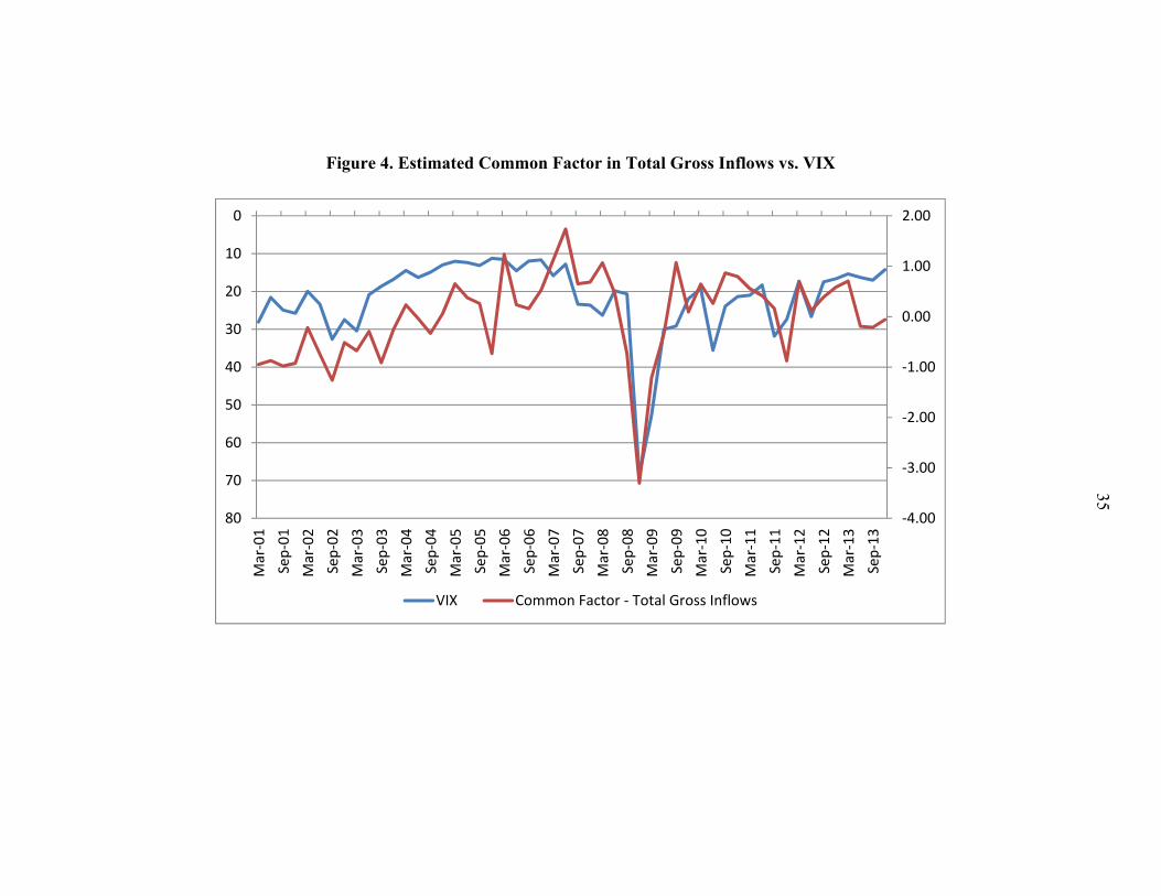
Figure 4. Estimated Common Factor in Total Gross Inflows vs. VIX

-4.00

-3.00

-2.00

-1.00

0.00

1.00

2.000

10

20

30

40

50

60

70

80

Mar

-01

Sep

-01

Mar

-02

Sep

-02

Mar

-03

Sep

-03

Mar

-04

Sep

-04

Mar

-05

Sep

-05

Mar

-06

Sep

-06

Mar

-07

Sep

-07

Mar

-08

Sep

-08

Mar

-09

Sep

-09

Mar

-10

Sep

-10

Mar

-11

Sep

-11

Mar

-12

Sep

-12

Mar

-13

Sep

-13

VIX Common Factor - Total Gross Inflows

35

Figure 5. The Model vs. the GFC and vs. the Taper Tantrum The left panel reports the cumulative drop in Equity (Bond or Bank) inflows for each EMs during the GFC against the corresponding beta coefficient (on the y-axis, as presented in Section 3 and Figure 4). The right panel plots the same beta coefficient against the cumulative drop experienced in any given asset during the taper tantrum episode. In the case of the GFC, the cumulative drop is computed at the peak of the crisis, namely 2007 Q4 and 2008 Q1. In the case of the tantrum, because the retrenchment was experienced in June/July 2013 and was very short lived, some countries experienced a dip in 2013 Q3 whereas others were affected in 2013 Q4 (or both). To circumvent this issue, we measure the cumulative drop over the Taper Tantrum as the minimum value among these two quarters. Note however that although the other procedure yield different quantitative assessment of the dip experienced, the general picture is invariant to the method chosen.

36

s

37

37

Figure 6. Institutional Quality vs. Correlations

Figure 6 plots the proxies used for institutional quality against the BOP correlation with EPFR and BIS flows computed for each country in our sample. We use the ICRG Law and Order and Investor protection ratings to proxy for institutional quality. The first, second and third panel reports are dedicated to Equity, Bond and Bank correlations respectively.

Turkey

South AfricaArgentina

Brazil

Chile

Colombia

Mexico

Peru

Uruguay

Venezuela, Rep. Bol.

Israel

India

Indonesia

Korea, Republic of

Malaysia

Pakistan

Philippines

Thailand

Belarus Kazakhstan

Bulgaria

Russian Federation

China,P.R.: Mainland

Ukraine

Czech Republic

Slovak RepublicEstonia

Latvia

HungaryLithuania

Croatia

SloveniaPoland

Romania

12

34

5L

aw

an

d O

rde

r

-.5 0 .5 1EPFR Equity Correlation

Turkey

South Africa

Argentina

Brazil

Chile

Colombia

Mexico

Peru

Uruguay


Israel

India

Indonesia

Korea, Republic of

Malaysia

Pakistan

Philippines

Thailand

Belarus

Kazakhstan

Bulgaria

Russian Federation


Ukraine

Czech RepublicSlovak Republic

Estonia LatviaHungaryLithuania

Croatia

Slovenia

Poland

Romania

46

81

01

2In

vest

me

nt

Ris

k

-.5 0 .5 1EPFR Equity Correlation

38

Figure 6. Institutional Quality vs. Correlations…contd…

Turkey


Brazil

Chile

Colombia

Mexico

Peru

Uruguay


Israel

India

Indonesia

Korea, Republic of

Malaysia

Pakistan

Philippines

Thailand

Belarus Kazakhstan

Bulgaria

Russian Federation


Ukraine

Czech Republic


Latvia

HungaryLithuania

Croatia

SloveniaPoland

Romania

12

34

5L

aw

an

d O

rde

r

-.5 0 .5 1EPFR Bond Correlation

Turkey

South Africa

Argentina

Brazil

Chile

Colombia

Mexico

Peru

Uruguay


Israel

India

Indonesia

Korea, Republic of

Malaysia

Pakistan

Philippines

Thailand

Belarus

Kazakhstan

Bulgaria

Russian Federation


Ukraine


Estonia LatviaHungaryLithuania

Croatia

Slovenia

Poland

Romania

46

81

01

2In

vest

me

nt

Ris

k

-.5 0 .5 1EPFR Bond Correlation

Tur


Brazil

Chile

Colombia

Mexico

Peru

Uruguay


Israel

India

Indonesia

Korea, Republic of

Malaysi

Pakistan

Philippines

Thailand

BelarusKazakhstan

Bulgaria

Russian Federation


Ukraine

Czech Republic


Latvia

HungaryLithuania

Croatia

SloveniaPoland

Romania

12

34

5L

aw

an

d O

rde

r

-.5 0 .5BIS Bank Correlation

Tur

South Africa

Argentina

Brazil

Chile

Colombia

Mexico

Peru

Uruguay


Israel

India

Indonesia

Korea, Republic of

Malaysi

Pakistan

Philippines

Thailand

Belarus

Kazakhstan

Bulgaria

Russian Federation


Ukraine


EstoniaLatvia HungaryLithuania

Croatia

Slovenia

Poland

Romania

46

81

01

2In

vest

me

nt

Ris

k

-.5 0 .5BIS Bank Correlation

39 38

40

Annex I – Details on Market Structure Variables

Because not all variables are applicable (or available) for all assets classes, we provide below a summary of the variables chosen to proxy for these dimensions, as well as their definition. Sources are presented in Table 2.

Foreign Openness and Size measures are based on stock variables and are used to proxy for the amount of foreign funding received and the size of the local market, respectively. To distinguish between the local and the relative size of a given market, the stock of foreign equity (or bond) in any given country is normalized (i) by the GDP of the recipient market and (ii) by the total of foreign equity (or bond) into the 34 EMs considered in this paper.

Liquidity measures are standard and rely on trading data when available. In the case of Equity markets, we use the turnover ratio, measured by the total value of shares traded every year divided by the average market capitalization. Because trading statistics are not available for all 34 bond markets on a consistent basis, we proxy for the level of liquidity of bond markets by creating a dummy variable which captures the membership of country to the key EM benchmarks (EMBI for Bond markets and MSCI for Equity markets).

The Composition of the Foreign Investor Base captures two characteristics of the lender profile of EMs. First we control for the source of funds by computing the share of the total stock of foreign equity (or bond) funding that is coming from advanced economies.14 Second we proxy for the importance of international funds and international (or global) banks in the foreign investor base. Because a decomposition of BOP stocks or flows by type of lender type is not available however, we compute, for each country in our sample, the correlation between BOP recorded equity (or bond) flows and EPFR recorded flows, which capture flows from Mutual funds in advanced economies to (or out of) Emerging Markets. For Bank flows, we use BIS locational statistics and compute the correlation between BOP recorded bank flows and BIS recorded flows. In both cases we interpret a high correlation as a sign that aforementioned investors (funds and global banks) account for most of the movements in capital inflows to (or out of) any given economy. For details on EPFR and BIS datasets, their coverage and how they relate to BOP recorded flows, see Annex II.

14 This includes G10 countries as well as key financial or offshore centers (Luxembourg, Ireland, Cayman, Barbados, Bahamas, Cayman, Guernsey and Jersey).

41

Annex II – BOP Flows, EPFR Fund flows and BIS banking flows

This annex presents the key properties of the other capital flows dataset based on dealer data used in this paper, the EPFR global dataset and BIS locational Banking statistics, and their connection with BOP recorded flows. In both cases, we argue that using the correlation between each of these datasets and its counterpart in the BOP statistics approximates well the importance of such intermediaries in driving capital flows to Emerging Markets. To proxy for the importance of funds (in particular Mutual Funds) in driving portfolio flows recorded in the BOP, we use the EPFR global dataset. Since its creation, the EPFR global has been tracking the performance and asset allocation of a vast number of equity and debt funds domiciled in developed countries and important offshore financial centers. Over time, its coverage increased significantly, reaching currently a wide industry and geographic coverage. As of 2013, the EPFR global was collecting information from more than 29,000 equity funds and 18,000 fixed-income funds representing US$20 trillion of assets invested in over 80 mature and emerging markets. As a result of its extensive coverage and quality,15 the EPFR global has been widely used recent seminal contributions funds behavior, in particular in the “country flows” format used in this paper (e.g., Raddatz and Schmukler (2012), Jotikasthira et al. (2012), Fratzscher (2012) and other references therein). In particular, given that an overwhelming majority of funds followed by the EPFR global dataset (i) are located in Advanced economies and (ii) account for a significant share of the external funding received by EMs, the “country flows” dataset has proved to be a good (high frequency) proxy of total gross inflows in (or out) of Emerging countries. For instance, Miao and Pant (2012) showed that EPFR fund flows correlate well with BoP recorded capital flows into emerging markets, thereby suggesting that when funds play an important role in the foreign investor base of a given country, EPFR flows act as a timely and accurate proxy for overall portfolio flows. On the other hand, two important methodological issues prevent us from simply retrenching EPFR flows from BOP recorded flows to assess the importance of funds. First, EPFR only covers a fraction of the mutual fund industry. Second, because EPFR Fund flows are based on dealer transactions, recorded flows are not always consistent with the residency criteria used to record transactions in the BOP data. For instance, when a fund dedicated to India and located in the U.S. sells an Indian Bond to another non-resident (which is not covered by EPFR), this sale is recorded as an outflow from India in the EPFR data, but does not generate a negative inflow in India’s BOP. As a result, the discrepancy between BOP and EPFR flows can be large is some occasions (see Koepke and Mohammed, 2014) for a

15 The EPFR dataset has been found to be a reliable data source. Comparing TNAs (Total Net Assets) and monthly returns of a subsample of EPFR funds to CRSP mutual fund data, Jotikasthira et al. (2012) found only minor differences between EPFR and CRSP datasets. See Puy (2013) for a thorough discussion of EPFR dataset.

42

thorough discussion). Relying on the correlation, rather than share in gross inflows, allows us to circumvent these issues. To proxy the importance of global banks in driving non-resident gross inflows to banks, as recorded in the BOP, we use the BIS international banking statistics. The BIS international banking statistics (IBS) track internationally active banks’ foreign positions through two main datasets: the BIS Consolidated Banking Statistics (CBS) and the BIS Locational Banking Statistics (LBS). We use the BIS LBS instead of BIS CBS because the first dataset provides data following the same residency principle as the one used in BOP data (see Cerutti et al. 2012 for further details). LBS captures the cross-border positions of all banks—defined as “Deposit-taking corporations, except the central bank” in the Balance of Payments Manual (BPM6)—domiciled in the reporting area (about 40 countries, mostly advanced countries and financial centers), including gross position vis-à-vis their foreign affiliates, against borrower countries. From the LBS data, based on publically available data, it is possible to breakdown how much are the gross inflows going to the banking and non-banking sector of each borrower country. The evolution of the global banks’ claims (as reported by BIS) against the banking sector of each borrower country in our sample is the series that we correlate with Other Investment to banks in order to define the correlation variable used as proxy for the composition of the foreign investor base. Since LBS is largely reflecting the position of key major international banking centers (e.g. Minoiu and Reyes, 2013, find that the top globally connected lenders in the LBS dataset are the banks operating in Belgium, France, Germany, Japan, Switzerland, U.K., and U.S.) we interpret a high correlation between the selected LBS series and Other Investment to banks in a given EM country as signaling a larger activity of global banks in that borrower country. In addition to global banks, BOP figures also include non-banks and banks located outside BIS reporting countries (e.g. China) as lenders.

push factors and capital flows to emerging markets: why ... · imf working papers describe research...

Documents