Python

Pawel Lachowicz, PhD

QuantAtRisk eBooks

for Quants

Volume

Fundamentals of Python 3.5Fundamentals of NumPy

Standard Library

7

Table of Contents

Preface 11

About the Author 13

Acknowledgements 15

1. Python for Fearful Beginners………………….17 1.1. Your New Python Flight Manual 17 1.2. Python for Quantitative People 21 1.3. Installing Python 25

1.3.1. Python, Officially 25 1.3.2. Python via Anaconda (recommended) 29

1.4. Using Python 31 1.4.1. Interactive Mode 31 1.4.2. Writing .py Codes 31 1.4.3. Integrated Developments Environments (IDEs) 32

PyCharm 32 PyDev in Eclipse 34 Spyder 37 Rodeo 38 Other IDEs 39

2. Fundamentals of Python………………………41 2.1. Introduction to Mathematics 41

2.1.1. Numbers, Arithmetic, and Logic 41

Integers, Floats, Comments 41 Computations Powered by Python 3.5 43 N-base Number Conversion 44 Strings 45 Booleans 46 If-Elif-If 46

8

Comparison and Assignment Operators 47 Precedence in Python Arithmetics 48

2.1.2. Import, i.e. "Beam me up, Scotty!" 49 2.1.3. Built-In Exceptions 51 2.1.4. math Module 55 2.1.5. Rounding and Precision 56 2.1.6. Precise Maths with decimal Module 58 2.1.7. Near-Zero Maths 62 2.1.8. fractions and Approximations of Numbers 64 2.1.9. Formatting Numbers for Output 66

2.2. Complex Numbers with cmath Module 71 2.2.1. Complex Algebra 71 2.2.2. Polar Form of z and De Moivre’s Theorem 73 2.2.3. Complex-valued Functions 75 References and Further Studies 77

2.3. Lists and Chain Reactions 79 2.3.1. Indexing 81 2.3.2. Constructing the Range 82 2.3.3. Reversed Order 83 2.3.4. Have a Slice of List 85 2.3.5. Nesting and Messing with List’s Elements 86 2.3.6. Maths and statistics with Lists 88 2.3.7. More Chain Reactions 94 2.3.8. Lists and Symbolical Computations with sympy Module 98 2.3.9. List Functions and Methods 102 Further Reading 104

2.4. Randomness Built-In 105 2.4.1. From Chaos to Randomness Amongst the Order 105 2.4.2. True Randomness 106 2.4.3. Uniform Distribution and K-S Test 110 2.4.4. Basic Pseudo-Random Number Generator 114

Detecting Pseudo-Randomness with re and collections Modules 115

2.4.5. Mersenne Prime Numbers 123 2.4.6. Randomness of random. Mersenne Twister. 126

Seed and Functions for Random Selection 129

Random Variables from Non-Random Distributions 131

2.4.7. urandom 132 References 133 Further Reading 133

9

2.5. Beyond the Lists 135 2.5.1. Protected by Tuples 135

Data Processing and Maths of Tuples 135

Methods and Membership 137

Tuple Unpacking 138

Named Tuples 139 2.5.2. Uniqueness of Sets 139 2.5.3. Dictionaries, i.e. Call Your Broker 141

2.6. Functions 145 2.6.1. Functions with a Single Argument 146

2.6.2. Multivariable Functions 147 References and Further Studies 149

3. Fundamentals of NumPy for Quants………….151 3.1. In the Matrix of NumPy 151

Note on matplotlib for NumPy 153

3.2. 1D Arrays 155 3.2.1. Types of NumPy Arrays 155

Conversion of Types 156 Verifying 1D Shape 156 More on Type Assignment 157 3.2.2. Indexing and Slicing 157

Basic Use of Boolean Arrays 158 3.2.3. Fundamentals of NaNs and Zeros 159 3.2.4. Independent Copy of NumPy Array 160 3.2.5. 1D Array Flattening and Clipping 161 3.2.6. 1D Special Arrays 163

Array—List—Array 164 3.2.7. Handling Infs 164 3.2.8. Linear and Logarithmic Slicing 165 3.2.9. Quasi-Cloning of Arrays 166

3.3. 2D Arrays 167 3.3.1. Making 2D Arrays Alive 167 3.3.2. Dependent and Independent Sub-Arrays 169 3.3.3. Conditional Scanning 170 3.3.4. Basic Engineering of Array Manipulation 172

3.4. Arrays of Randomness 177 3.4.1. Variables, Well Shook 177

Normal and Uniform 177 Randomness and Monte-Carlo Simulations 179 3.4.2. Randomness from Non-Random Distributions 183

10

3.5. Sample Statistics with scipy.stats Module 185 3.5.1. Downloading Stock Data from Yahoo! Finance 186 3.5.2. Distribution Fitting. PDF. CDF. 187 3.5.1. Finding Quantiles. Value-at-Risk. 189

3.6. 3D, 4D Arrays, and N-dimensional Space 193 3.6.1. Life in 3D 194 3.6.2. Embedding 2D Arrays in 4D, 5D, 6D 196

3.7. Essential Matrix and Linear Algebra 203 3.7.1. NumPy’s ufuncs: Acceleration Built-In 203 3.7.2. Mathematics of ufuncs 205 3.7.3. Algebraic Operations 208

Matrix Transpositions, Addition, Subtraction 208 Matrix Multiplications 209 @ Operator, Matrix Inverse, Multiple Linear Regression 210 Linear Equations 213 Eigenvectors and Principal Component Analysis (PCA) for N-Asset Portfolio 215

3.8. Element-wise Analysis 223 3.8.1. Searching 223 3.8.2. Searching, Replacing, Filtering 225 3.8.3. Masking 227 3.8.4. Any, if Any, How Many, or All? 227 3.8.5. Measures of Central Tendency 229

Appendixes……………………………………….231 A. Recommended Style of Python Coding 231 B. Date and Time 232 C. Replace VBA with Python in Excel 232 D. Your Plan to Master Python in Six Months 233

11

Preface This is the first part out of the Python for Quants trilogy, the book-series that provides you with an opportunity to commence your programming experience with Python—a very modern and dynamically evolving computer language. Everywhere.

This book is completely different than anything ever written on Python, programming, quantitative finance, research, or science. It became one of the greatest challenges in my career as a writer—being able to deliver a book that anyone can learn programming from in the most gentle but sophisticated manner—starting from absolute beginner. I made a lot of effort not to follow any rules in book writing, solely preserving the expected skeleton: chapters, sections, margins.

It is written from a standpoint of over 21 years of experience as a programmer, with a scientific approach to the problems, seeking pinpoint solutions but foremost blended with a heart and soul—two magical ingredients making this book so unique and alive.

It is all about Python strongly inclined towards quantitative and numerical problems. It is thought of quantitative analysts (also known as quants) occupying all rooms from bedrooms to Wall Street trading rooms. Therefore, it is written for traders, algorithmic traders, and financial analysts. All students and PhDs. In fact, for anyone who wishes to learn Python and apply its mathematical abilities.

In this book you will find numerous examples taken from finance, however the content is not strictly limited to that one single field. Again, it is all about Python. From the beginning to the end. From the tarmac to the stratosphere of dedicated programming.

Within Volume I, we will try to cover the quantitative aspects of Fundamentals of Python supplemented with most useful language’s structures taken from the Python’s Standard Library. We will be studying the numerical and algebraical concepts of NumPy to equip you with the best of Python 3.5. Yes, the newest version of the interpreter. This book is up to date.

12

If you hold a copy of this ebook it means you are very serious about learning Python quickly and efficiently. For me it is a dream to guide you from cover to cover, leaving you wondering "what’s next?", and making your own coding in Python a truly remarkable experience. Volume I is thought of as a story on the quantitatively dominated side of Python for beginners which, I do hope, you will love from the very first page.

If I missed something or simply left anything with a room for improvement—please email me at pawel@quantatrisk.com. The 1st edition of Volume II will come out along with the 2nd edition of Volume I. Thank you for your feedback in advance.

Ready for Python for Quants fly-thru experience? If so, fasten your seat belt and adjust a seat to an upright position. We are now clear for take-off!

Enjoy your flight!

Paweł Lachowicz, PhD November 26th, 2015

13

About the Author

Paweł Lachowicz was born in Wrocław, Poland in 1979. At the age of twelve he became captivated by programming capability of the Commodore Amiga 500. Over the years his mind was sharply hooked on maths, physics, and computer science, concurrently exploring the frontiers of positive thinking and achieving "the impossible" in life. In 2003 he graduated from Warsaw University defending his MSc degree in astronomy; four years later—a PhD degree in signal processing applied directly to black-hole astrophysics at Polish Academy of Sciences in Warsaw, Poland. His novel discoveries secured his post-doctoral research position at the National University of Singapore in 2007. In 2010 Pawel shifted his interest towards financial markets, trading, and risk management. In 2012 he founded QuantAtRisk.com portal where he continuously writes on quantitative finance, risk, and applied Python programming.

Today, Pawel lives in Sydney, Australia (dreaming of moving to Singapore or to the USA) and serves as a freelance financial consultant, risk analyst, and algorithmic trader. Worldwide. Relaxing, he fulfils his passions as a writer, motivational speaker, yacht designer, photographer, traveler, and (sprint) runner.

He never gives up.

58

A superbly handy function in math arsenal is trunc which provides a stiff separation of the real number from its fractional part: >>> e 2.718281828459045 >>> y = trunc(e) 2 >>> type(y) <class 'int'> >>> y == floor(e) True

where the last logical test is positive despite the type of y is an integer and floor(e) is a float. It is always better to use trunc than floor function if you want to get the real value of your number. In certain cases (big numbers) rounding to the floor may fail. That is why the trunc function is a perfect choice.

2.1.6. Precise Maths with decimal Module

Python’s Standard Library goes one step forward. It grants us access to its another little pearl known as decimal module. Now the game is all about precision of calculations. When we use floating-point mathematical operations usually we do not think how computer represents the floats in its memory. The truth is a bit surprising when you discover that:

>>> r = 0.001 >>> print("r= %1.30f" % r) # display 30 decimal places r= 0.001000000000000000020816681712 instead of

r= 0.001000000000000000000000000000 It is just the way it is: the floats are represented in a binary format that involves a finite number of bits of their representation. When used in calculations, the floats provide us with a formal assurance up to 17 decimal places. However, the rest is not ignored and in case of heavy computations those false decimal digits may propagate. In order to “see” it—run the following code:

r = 0.001 t = 0.002 print("r = %1.30f" % r) print("t = %1.30f" % t) print("r+t = %1.30f" % (r+t)) You should get:

r = 0.001000000000000000020816681712 t = 0.002000000000000000041633363423 r+t = 0.003000000000000000062450045135 It is now clear how those “happy endings” accumulate an error. The question you may ask is: “Should I be worried about that?”

trunc()

Code 2.6

In many cases the function of trunc can be replaced with the operation of the floor division:

from math import trunc from random import random as r x = r()*100 # float print(x//1 == trunc(x))

True

thought the former returns a float and trunc an integer if x is float.

You may obtain a pure fractional part of the float as follows, e.g:

>>> from math import pi >>> pi 3.141592653589793 >>> pi - pi//1 0.14159265358979312

79

2.3. Lists and Chain Reactions

Python introduces four fundamental data structures: lists, tuples, sets, and dictionaries. When encountered for the very first time, the concept may cause mixed feelings on data aggregation, manipulation, and their use. As a beginner in Python you just need to take a leap of faith that such clever design, in fact, pays huge dividends in practice. For many reasons and by many people Python’s lists are considered as one of the language’s greatest assets. You can think of lists as of data collectors or containers. The fundamental structure is a sequence, e.g. of numbers, strings, or a mix of numbers and strings. Data are then organised in a given order and each element of such data sequence has its assigned position, thus an index. By making a reference by index we gain an immediate access to data or sub-data structures in a given list.

Not only we can build single lists containing data of different types but also use them concurrently to generate new lists or to gather results from (many) numerical calculations in one place. I dare to call this process—the chain reactions—a bit of nuclear power of Python at your private disposal.☺

The Python’s lists may seem a bit uncomfortable in the beginning. This are two reasons: (a) the indexing starts from zero and not from one; (b) slicing the list requires an odd use of indexing. The pain vanishes with practice and those two obstacles become your natural instinct.

Similarly as applied in C++ or Java languages, the indexing starting at 0th-position is highly unnatural. We usually do not start the counting process of fruits in a box from zero, right? The only example that could justify counting something from zero is: money in your wallet. First, you have nothing: >>> wallet = [] # an empty list in Python; square brackets >>> wallet [] >>> type(wallet) <class 'list'>

or >>> wallet = [None]; wallet [None]

where None is of <class 'NoneType'>. Next, you earn $1.50 by selling, say, an apple to your first customer and you jot this transaction down (add it to your Python’s list) for the record: >>> wallet = [None, 1.50] >>> wallet[0] # there is no physical value assigned >>> wallet[1] # index=1 :: 2nd position in the list 1.5

80

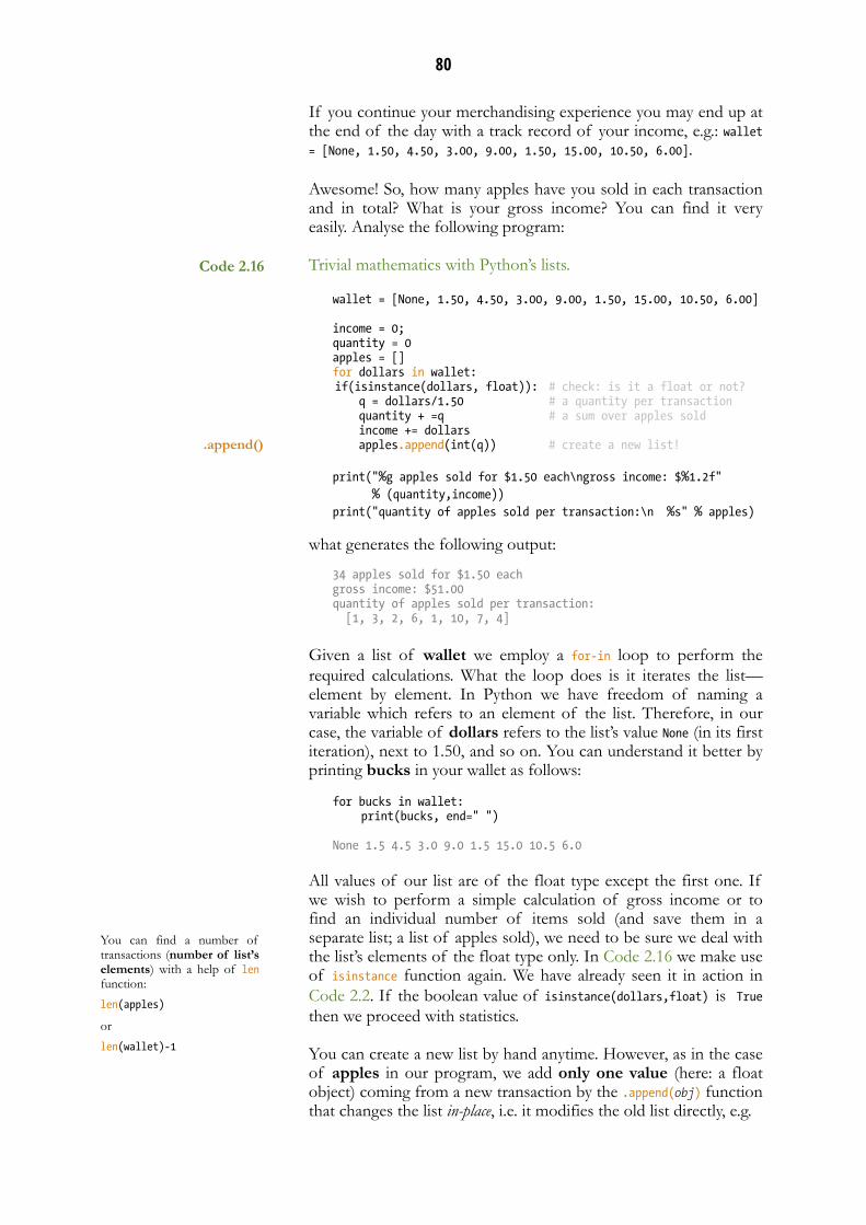
If you continue your merchandising experience you may end up at the end of the day with a track record of your income, e.g.: wallet = [None, 1.50, 4.50, 3.00, 9.00, 1.50, 15.00, 10.50, 6.00].

Awesome! So, how many apples have you sold in each transaction and in total? What is your gross income? You can find it very easily. Analyse the following program:

Trivial mathematics with Python’s lists. wallet = [None, 1.50, 4.50, 3.00, 9.00, 1.50, 15.00, 10.50, 6.00]

income = 0; quantity = 0 apples = [] for dollars in wallet: if(isinstance(dollars, float)): # check: is it a float or not? q = dollars/1.50 # a quantity per transaction quantity + =q # a sum over apples sold income += dollars apples.append(int(q)) # create a new list!

print("%g apples sold for $1.50 each\ngross income: $%1.2f" % (quantity,income)) print("quantity of apples sold per transaction:\n %s" % apples) what generates the following output:

34 apples sold for $1.50 each gross income: $51.00 quantity of apples sold per transaction: [1, 3, 2, 6, 1, 10, 7, 4]

Given a list of wallet we employ a for-in loop to perform the required calculations. What the loop does is it iterates the list—element by element. In Python we have freedom of naming a variable which refers to an element of the list. Therefore, in our case, the variable of dollars refers to the list’s value None (in its first iteration), next to 1.50, and so on. You can understand it better by printing bucks in your wallet as follows:

for bucks in wallet: print(bucks, end=" ")

None 1.5 4.5 3.0 9.0 1.5 15.0 10.5 6.0

All values of our list are of the float type except the first one. If we wish to perform a simple calculation of gross income or to find an individual number of items sold (and save them in a separate list; a list of apples sold), we need to be sure we deal with the list’s elements of the float type only. In Code 2.16 we make use of isinstance function again. We have already seen it in action in Code 2.2. If the boolean value of isinstance(dollars,float) is True then we proceed with statistics.

You can create a new list by hand anytime. However, as in the case of apples in our program, we add only one value (here: a float object) coming from a new transaction by the .append(obj) function that changes the list in-place, i.e. it modifies the old list directly, e.g.

You can find a number of transactions (number of list’s elements) with a help of len function:

len(apples)

or

len(wallet)-1

.append()

Code 2.16

97

You may get a completely different outcome if you generate lst as:

lst = [[i, stock, price] for i in range(1, n+1) \ for stock in tickers \ for price in [randomprice()*n]]

what would cause a triple loop over all possible elements.

As a supplement to the abovementioned code, it is a slightly modified version (for a single stock only) that might look like this:

import random from datetime import datetime, timedelta

def randomprice(): return random.uniform(115, 121) # float

def randomvolume(): return random.randrange(100000, 1000000) # integer

lst2 = [[(datetime.now()+timedelta(days=i)).strftime("%d-%m-%Y"), stock, price, volume] \ for i in range(10) \ for stock in ['AAPL'] \ for price in [randomprice()] \ for volume in [randomvolume()]] print(lst2)

[['08-05-2015','AAPL', 119.36081566260756, 771321], ['09-05-2015', 'AAPL', 118.89791980293758, 142487], ['10-05-2015', 'AAPL', 115.78468917663126, 771096], ['11-05-2015', 'AAPL', 119.37994620603668, 936208], ['12-05-2015', 'AAPL', 118.92154718243538, 540723], ['13-05-2015', 'AAPL', 119.59934410132043, 242330], ['14-05-2015', 'AAPL', 119.29542558713318, 725599], ['15-05-2015', 'AAPL', 117.59180568515953, 465050], ['16-05-2015', 'AAPL', 115.18821876802848, 771109], ['17-05-2015', 'AAPL', 118.07603557924027, 408705]]

Above, we added more functionality from the Standard Library in the form of a (formatted) string storing a date. Without additional documentation on the datetime module you may decipher that we are using a running index i from 0 to 9 as a forward-looking time delay: the first entry is as for "now", i.e. for a current date (e.g., "08-05-2015") and the following nine dates are shifted by i i.e. by 1, 2, …, 9 days. The function .strftime("%d-%m-%Y") helps us to convert the datetime object into a readable date (a string variable).

Having that, the quickest way to extract a list of prices or volumes is via an alternative application of the zip function—the argument unpacking:

date, _, prices, vol = zip(*lst2) # use _ to skip a sublist print(list(prices[-3:]))

[117.59180568515953, 115.18821876802848, 118.07603557924027]

where we displayed last three stock prices from the unpacked list of prices. In addition, if you look for the day when the volume was largest, try to add:

zip(*list) Argument unpacking for lists

datetime is a handy module to convert or combine time and dates into more useful forms. We will cover it in greater detail within Appendix. For now, a few examples:

>>> d = datetime.now() >>> d datetime.datetime(2015, 7, 7, 12, 42, 5, 384105) >>> d.year 2015 >>> d + timedelta(seconds=-11) datetime.datetime(2015, 7, 7, 12, 41, 54, 384105)

Code 2.21

189

mu_fit2, sig_fit2 = -0.0000, 1.0000

as expected. As far as the numbers are lovely, the picture tells a whole story. Extending further 3.9: # --Plotting PDFs fig, ax1 = plt.subplots(figsize=(10, 6)) # plt.subplot(211) plt.hist(ret, bins=50, normed=True, color=(.6, .6, .6)) plt.hold(True) plt.axis("tight") plt.plot(x, pdf, 'r', label="N($\mu_{fit}$,$\sigma_{fit}$)") plt.legend() # plt.subplot(212) plt.hist(z, bins=50, normed=True, color=(.6, .6, .6)) plt.axis("tight") plt.hold(True) plt.plot(x, stdpdf, 'b', label="N($\mu_{fit2}$,$\sigma_{fit2}$) = N(0,1)") plt.legend() plt.show()

we combine both pdf ’s with the original (upper) and transformed (bottom) MA daily returns distributions (see the chart above).

3.5.3. Finding Quantiles. Value-at-Risk.

The starting point is trivial. For any given distribution, k is called α-quantile such:

It means that in case of the Normal distribution, we have to perform the integration in the interval:

Pr(X < k) = ↵

190

To 3.9, we add:

# --Finding k such that Pr(X<k)=alpha given alpha alpha = 0.05 k = norm.ppf(alpha, mu_fit, sig_fit) print("\nk = %.5f" % k)

where .ppf function stands for the inverse of the cumulative density function or percent point function (ppf). The task can be reversed and formulated as follows: given k find α. In Python we solve it by:

# --Finding Pr(X<k) given k pr = norm.cdf(k, mu_fit, sig_fit) print("Pr(X<k) = %.5f" % pr)

what delivers the output:

k = -0.02753 Pr(X<k) = 0.05000

if the same value of k is used for the latter computation. This result, derived here based on MA stock data, simply communicates that there is 5% of chances that on the next day, MA may lose 2.75% or more. Saying so, in fact, we define a quantitative measure of risk—VaR or Value-at-Risk described more formally as:

where by L we denote a loss (in percent) that an asset can experience on the next day. Having that, there are at least two methods of finding VaR for the sample data: analytical and empirical.

The analytical way is based on (1) fitting the distribution with the model, e.g. the Normal distribution, and (2) finding α-quantile or, saying in terms of finance, (1-α)VaR, based on the model integration as have performed above. The empirical method is through a "manual" integration of the distribution. It requires a design of a special custom function:

def findvar(ret, alpha=0.05, nbins=200): # Function computes the empirical Value-at-Risk (VaR) for # return-series # (ret) defined as NumPy 1D array, given alpha # # compute a normalised histogram (\int H(x)dx = 1) # nbins: number of bins used (recommended nbins>50) hist, bins = np.histogram(ret, bins=nbins, density=True) wd = np.diff(bins) # resolution of H(x) # cumulative sum from -inf to +inf cumsum = np.cumsum(hist * wd) # find an area of H(x) for computing VaR crit = cumsum[cumsum <= alpha] n = len(crit) # (1-alpha)VaR VaR = bins[n] return VaR

.ppf

Pr(L �VaR1�↵) = ↵

np.histogram

np.cumsum

Z k

�1N(x;µ,�)dx = ↵

203

3.7. Essential Matrix and Linear Algebra

3.7.1. NumPy’s ufuncs: Acceleration Built-In

When you buy a nice car with 300 horsepower under the hood, you expect it to perform really well in most road conditions. The amount of torque combined with a high-performance engine gives you a lot of thrust and confidence while overtaking. The same level of expectations arises when you decide, from now on, to use Python for your numerical computations.

Everyone heard about highly efficient engines of C, C++, or Fortran when it comes to the speed of the code execution. A magic takes place while the code is compiled to its machine-digestible version in order to gain the noticeable speed-ups. The trick is that within these languages every variable is declared, i.e. its type is known in advance before any mathematical operation begins. This is not the case of Python where variables are checked on-the-way as the interpreter reads the code. For example, if we declare:

r = 7

Python checks the value on the right-hand side first and if it does not have a floating-point representation, it will assume and remember that r is an integer. So, what does it have to do with the speed? Analyse the following case study.

Let’s say we would like to compute the values of the function:

for a grid of x defined between 0.00001 and 100 with the resolution of 0.00001. Based on our knowledge till now, we can find all corresponding solutions using at least two methods: list and loop or list comprehension. The third method employs so-called NumPy’s universal functions (or ufuncs for short). As we will see below, the former two methods are significantly slower than the application of ufuncs. The latter performs vectorised operations on arrays, i.e. a specific ufunc applies to each element. Since the backbone of ufuncs is CPython, the performance of our engine is optimised for speed.

Compute f(x) as given above using three different methods: (1) list and loop, (2) list comprehension, and (3) NumPy’s ufuncs. Measure and compare the time required to reach the end result.

from math import sin, cos, exp, pi, sqrt, pow from time import time import numpy as np from matplotlib import pyplot as plt

def fun(x): return sqrt(abs(sin(x-pi)*pow(cos(x+pi), 2)) * (1+exp(-x/ sqrt(2*pi))))

Code 3.12

f(x) =

r|sin(x� ⇡) cos

2(x+ ⇡)|

⇣1 + e

�xp2⇡

⌘