quantitative analysis of computer interaction movements
TRANSCRIPT

Quantitative analysis of computer interaction movements
Citation for published version (APA):Nieuwenhuizen, C. J. H. (2015). Quantitative analysis of computer interaction movements. TechnischeUniversiteit Eindhoven.
Document status and date:Published: 01/01/2015
Document Version:Publisher’s PDF, also known as Version of Record (includes final page, issue and volume numbers)
Please check the document version of this publication:
• A submitted manuscript is the version of the article upon submission and before peer-review. There can beimportant differences between the submitted version and the official published version of record. Peopleinterested in the research are advised to contact the author for the final version of the publication, or visit theDOI to the publisher's website.• The final author version and the galley proof are versions of the publication after peer review.• The final published version features the final layout of the paper including the volume, issue and pagenumbers.Link to publication
General rightsCopyright and moral rights for the publications made accessible in the public portal are retained by the authors and/or other copyright ownersand it is a condition of accessing publications that users recognise and abide by the legal requirements associated with these rights.
• Users may download and print one copy of any publication from the public portal for the purpose of private study or research. • You may not further distribute the material or use it for any profit-making activity or commercial gain • You may freely distribute the URL identifying the publication in the public portal.
If the publication is distributed under the terms of Article 25fa of the Dutch Copyright Act, indicated by the “Taverne” license above, pleasefollow below link for the End User Agreement:www.tue.nl/taverne
Take down policyIf you believe that this document breaches copyright please contact us at:[email protected] details and we will investigate your claim.
Download date: 06. Feb. 2022

QUANTITATIVE ANALYSIS OF COMPUTER INTERACTION
MOVEMENTS
Karin NieuwenhuizenQ
UA
NTITA
TIVE
AN
ALY
SIS O
F CO
MP
UT
ER
INT
ER
AC
TIO
N M
OV
EM
EN
TS K
AR
IN N
IEU
WE
NH
UIZ
EN
ISBN: 978-90-386-3839-3ISBN: 978-90-386-3839-3
QUANTITATIVE ANALYSIS
OF COMPUTER INTERACTION MOVEMENTS
Op woensdag 13 mei 2015 om 16.00 uur vindt de
promotie plaats in zaal 4 van het Auditorium van
de TU/e.
Aansluitend is er een receptie waarvoor u van
harte bent uitgenodigd.
Karin Nieuwenhuizen
tot het bijwonen van de openbare
verdediging van mijn proefschrift
UITNODIGING

Quantitative analysis of computer InteractIon
movements

A catalogue record is available from the Eindhoven University of Technology Library
ISBN: 978-90-386-3839-3
Cover design and layout: Saskia RendersPrinted by: Gildeprint Drukkerijen
© Karin Nieuwenhuizen, 2015
All rights reserved. No part of this book may be reproduced or transmitted in any form or by any means, electronic or mechanical, including photocopying, recording, or by any information storage and retrieval system, without permission from the author.
ter verkrijging van de graad van doctor aan de Technische Universiteit Eindhoven, op gezag van
de rector magnificus prof.dr.ir. F.P.T. Baaijens, voor een commissie aangewezen door het College voor Promoties,
in het openbaar te verdedigen op woensdag 13 mei 2015 om 16:00 uur
door
Catharina Johanna Henrieke Nieuwenhuizen
geboren te Geldrop
Quantitative analysis of computer InteractIon
movements
proefschrift

Dit proefschrift is goedgekeurd door de promotoren en de samenstelling van de promotiecommissie is als volgt:
voorzitter: prof.dr.ir. A.C. Brombacher1e promotor: prof.dr.ir. J.B.O.S. Martens2e promotor: prof.dr.ir. R. van Liereleden: prof. R. Balakrishnan (University of Toronto) prof.dr. D.V. Keyson (Technische Universiteit Delft) prof.dr. W.A. IJsselsteijn prof.dr.ir. J.H. Eggen

Table of contents
introduction 71.1 3D user interfaces 81.2 Evaluation frameworks 111.3 Research approach 131.4 Research objectives 141.5 Thesis outline 14
interaction task design 172.1 3D interaction tasks 182.2 Goal-directed movement tasks 212.3 Experimental set-up 28
Performance characterization: Fitts’ law 353.1 Task performance characterization 363.2 Experiment 443.3 Conclusion & discussion 63
Movement characterization 674.1 Measures characterizing movement quality 684.2 Selection procedure to reduce number of measures 764.3 Experiment 784.4 Conclusion & discussion 99
Movement phases 1035.1 Division in movement phases 1045.2 Explorative study 1055.3 Movement parsing method 1125.4 Experiment 1145.5 Conclusion & discussion 139
application to 3D environment 1436.1 3D movements 1446.2 Experiment 1476.3 Conclusion & discussion 158
Conclusions and future directions 1617.1 Summary of contributions 1627.2 Research conclusions 1637.3 Future directions 167
References 173
appendices 185A.1 Phase-based measures 186A.2 Clustering selection task 187A.3 Clustering tracing task 189A.4 Measures 3D steering movement 191

Chapter 1
Introduction
Chapter 18
“For many years, the field of VEs and 3D UIs were so novel and the possibilities so limitless that many researchers simply focused on developing new devices, interaction techniques, and UI metaphors – exploring the design space – without taking the time to assess how good the new designs were.“ (Bowman, Kruijff, LaViola, & Poupyrev, 2004)
Several researchers in the field of 3D interaction have not only argued for a common focus with respect to the development of 3D interactive systems but also for a common research focus to evaluate these systems in a systematic way (Bowman et al., 2004; Gabbard, Hix, & Swan, 1999; Grissom & Perlman, 1995; Poupyrev, Weghorst, Billinghurst, & Ichikawa, 1997). Nevertheless, most experimental studies in which input devices, interaction techniques and system parameters are evaluated represent idiosyncratic characteristics of the available systems. In this thesis we will take a first step towards developing a more thorough and standardized method for the quantitative evaluation of spatial input devices and interaction techniques used especially in mixed reality (MR) desktop systems.
1.1 3D user interfaces
1.1.1 Mixed reality environmentsMost computer interactions occur via a direct manipulation interface, also called a WIMP (Windows, Icons, Menu, Pointer) interface. The most obvious way to improve human-computer interaction is to create specialized input devices and interaction techniques to use in combination with WIMP interfaces. A more challenging approach is to develop new interfaces with interaction styles more closely related to real-world interactions – also called post-WIMP interfaces – such as MR desktop systems.
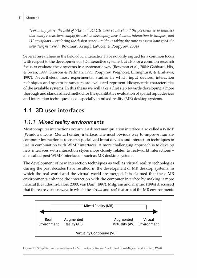
The development of new interaction techniques as well as virtual reality technologies during the past decades have resulted in the development of MR desktop systems, in which the real world and the virtual world are merged. It is claimed that these MR environments enhance the interaction with the computer interface by making it more natural (Beaudouin-Lafon, 2000; van Dam, 1997). Milgram and Kishino (1994) discussed that there are various ways in which the virtual and real features of the MR environments
Figure 1.1. Simplified representation of a “virtuality continuum” (adopted from Milgram and Kishino, 1994)

Introduction 9
can be combined along a virtuality continuum (see Figure 1.1), which results in different MR desktop interfaces. Several examples of these MR desktops are the Personal Space Station (Mulder & Van Liere, 2002), Virtual Interaction Platform (Aliakseyeu, Martens, Subramanian, Vroubel, & Wesselink, 2001), MagicBook (Billinghurst, Kato, & Poupyrev, 2001), LivePaper (Robinson & Robertson, 2001), DigitalDesk (Wellner, 1993), and LiveBoard (Elrod et al., 1992).
What the above-mentioned MR desktop environments have in common is that real physical objects in the user’s environment play a role in the interaction. For example, the MagicBook uses a real book to let people interact with the three-dimensional (3D) virtual models that are appearing out of the pages (Billinghurst et al., 2001). The Personal Space Station (PSS) supports direct interaction with 3D data with the help of several graspable input devices, like a thimble device, a cutting plane device, a ruler device and a cube device (Mulder & Van Liere, 2002). The design of these mixed reality systems do not only require the design of new input devices but also the design of new interaction styles. For example, LivePaper, LiveBoard and DigitalDesk are stylus-based display systems, in which the pen allows for button-click interactions as well as gesture-based interactions (Elrod et al., 1992; Robinson & Robertson, 2001; Wellner, 1993). Also the Virtual Interaction Platform (VIP) allows for a different way of interacting with the computer by supporting bi-manual interactions (Aliakseyeu et al., 2001).
These interaction styles are more intuitive because they let people apply their existing skills by interacting with everyday objects. However, this in itself doesn’t guarantee improved performance; amongst other things, we still need systematic ways to assess the performance of these new interaction techniques.
1.1.2 Usability evaluationAn important aspect that should be taken into account when designing MR desktop systems is its usability:
“The extent to which a product can be used by specified users to achieve specified goals with effectiveness, efficiency and satisfaction in a specified context of use.” (ISO 9241-11, 1998)
To design spatial interaction systems (such as MR desktop systems) that are easy to use and learn, an iterative design approach should be followed in which the user is involved throughout the process (Bowman et al., 2004; Gabbard et al., 1999).
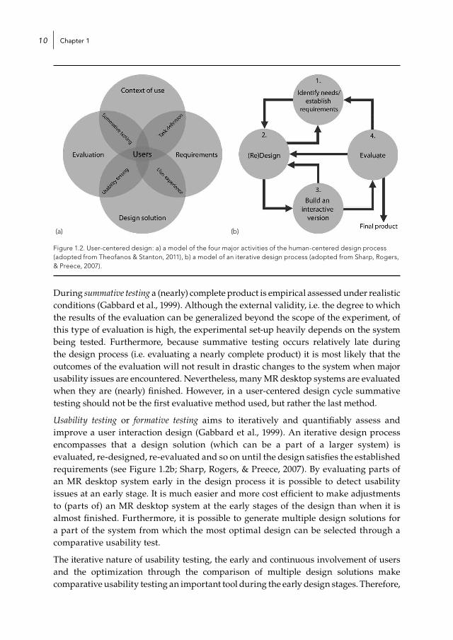
Most models of the human-centered design process contain four major activities: understanding context of use, specifying requirements, producing design solutions and evaluating designs. Figure 1.2a shows these activities of the human-centered design process and how they are overlapping in time and scope (Theofanos & Stanton, 2011). In this diagram two different evaluation approaches are presented: summative testing (overlap between evaluation and context of use) and usability testing (overlap between design solution and evaluation).
Chapter 110
During summative testing a (nearly) complete product is empirical assessed under realistic conditions (Gabbard et al., 1999). Although the external validity, i.e. the degree to which the results of the evaluation can be generalized beyond the scope of the experiment, of this type of evaluation is high, the experimental set-up heavily depends on the system being tested. Furthermore, because summative testing occurs relatively late during the design process (i.e. evaluating a nearly complete product) it is most likely that the outcomes of the evaluation will not result in drastic changes to the system when major usability issues are encountered. Nevertheless, many MR desktop systems are evaluated when they are (nearly) finished. However, in a user-centered design cycle summative testing should not be the first evaluative method used, but rather the last method.
Usability testing or formative testing aims to iteratively and quantifiably assess and improve a user interaction design (Gabbard et al., 1999). An iterative design process encompasses that a design solution (which can be a part of a larger system) is evaluated, re-designed, re-evaluated and so on until the design satisfies the established requirements (see Figure 1.2b; Sharp, Rogers, & Preece, 2007). By evaluating parts of an MR desktop system early in the design process it is possible to detect usability issues at an early stage. It is much easier and more cost efficient to make adjustments to (parts of) an MR desktop system at the early stages of the design than when it is almost finished. Furthermore, it is possible to generate multiple design solutions for a part of the system from which the most optimal design can be selected through a comparative usability test.
The iterative nature of usability testing, the early and continuous involvement of users and the optimization through the comparison of multiple design solutions make comparative usability testing an important tool during the early design stages. Therefore,
(a) (b)
Figure 1.2. User-centered design: a) a model of the four major activities of the human-centered design process (adopted from Theofanos & Stanton, 2011), b) a model of an iterative design process (adopted from Sharp, Rogers, & Preece, 2007).

Introduction 11
we will focus on this type of usability tests for the development of a methodology to assess the performance of (parts of) MR desktop systems.
1.2 evaluation frameworksIn the late 1990s several 3D interaction researchers have proposed frameworks for the evaluation of 3D interaction techniques (Bowman & Hodges, 1999; Gabbard et al., 1999; Poupyrev et al., 1997). Figure 1.3a illustrates the testbed evaluation proposed by Bowman and Hodges (1999) and Figure 1.3b illustrates the sequential evaluation methodology proposed by Gabbard et al. (1999). Poupyrev et al. (1997) proposed a conceptual framework for immersive direct manipulation called VRMAT (Virtual Reality Manipulation Assessment Testbed). Two important steps these three evaluation methodologies have in common are the development of a taxonomy for interaction techniques or tasks and the definition of performance criteria.
(a) (b)
Figure 1.3. Frameworks for the evaluation of 3D interaction techniques: a) testbed evaluation (adopted from Bowman, Kruijff, LaViola, & Poupyrev, 2004), and b) sequential evaluation methodology (adopted from Gabbard, Hix & Swan, 1999).
1.2.1 TaxonomyTo evaluate parts of 3D interaction systems, such as input devices and interaction techniques, in a systematic way standardized and representative tasks are required. It is argued that each complex spatial interaction task is composed of the same basic interaction tasks, which can be identified by means of a task analysis (Bowman et al., 2004; Gabbard et al., 1999; Poupyrev et al., 1997). The resultant taxonomy of basic
Chapter 112
interaction tasks is useful for the definition of representative experimental tasks that can be used in the systematic evaluation of input devices and interaction techniques used, for example, in MR desktop systems.
Foley, Wallace and Chan (1984) suggested that each 2D interaction sequence could be decomposed into a series of basic interaction tasks. They identified the following basic 2D interactions: a) select, b) position, c) orient, d) path, e) quantify, and f) text. Based on this task analysis Poupyrev et al. (1997) incorporated three basic tasks in their testbed, namely selection, position and orientation tasks. In addition, this 2D task decomposition served as a basis for the taxonomy of 3D interaction techniques proposed by Bowman and Hodges (1999), which also includes selection, position and orientation as the main spatial interaction tasks. Together with the description of the task parameters, which can influence the user performance on spatial selection, position and orientation tasks (Poupyrev et al., 1997), these taxonomies provide a good starting point for the development of experimental tasks to evaluate 3D computer interactions.
1.2.2 Performance assessmentAnother important aspect of a usability evaluation is the performance assessment. In this thesis we will focus on the user’s task performance.
1.2.2.1 Performance metricsThe three evaluation frameworks included only a limited number of task performance measures which are related to speed and accuracy (Bowman & Hodges, 1999; Gabbard et al., 1999; Poupyrev et al., 1997). Time is used to determine the performance speed and the number of errors or the proximity to the desired position or orientation is used to determine the accuracy of the task performance. These measures are often the only measures used in the evaluation of MR desktop systems and we believe that additional measures should be used to gain more profound insight into the way input devices and interaction techniques are used.
In our opinion, considerably more information can be derived from the interaction movements that can assist in understanding why a certain input device or interaction technique is faster in use than another one. Insights with respect to how interaction movements are carried out can not only help explaining differences between input devices or interaction techniques, but can also reveal opportunities to further improve the designs that are being evaluated. Aspects of the interaction movements that should be taken into account, besides speed and accuracy, are the smoothness of the traveled path and the smoothness of the displacement over time. In our opinion, high quality interaction movements are fast, without any perturbations in the traveled path and the velocity course.

Introduction 13
1.2.2.2 Performance modelsNot only additional quantitative measures can provide more insight with respect to the interaction movements, but also the development or optimization of performance models. Performance models “aim to predict the performance of a user on a particular task within the interface” (Bowman et al., 2004). A well-known performance model is Fitts’ law which predicts the time required to rapidly move to a target area as a function of the target distance and the target size. A different approach towards Fitts’ law modeling by means of a slightly more complex model might result in a more accurate description of the speed-accuracy relationship as well as a better fit of the data and a better discrimination between experimental conditions.
In this thesis we will show that the optimization of the Fitts’ law performance model and the use of additional performance measures (derived from the traveled path and the velocity course) will result in more accurate descriptions of interaction movements. More insight into the produced interaction movements can help designers and researchers to better understand the differences and commonalities between input devices and interaction techniques that are being evaluated. We believe that this deepened understanding of interaction movements is valuable input to further improve the input devices and interaction techniques used in MR desktop systems.
1.3 Research approachAlthough the end goal is a complete methodology to systematically evaluate the performance of spatial input devices and interaction techniques we acknowledge that in this thesis we can only take a first step towards developing such a methodology. As mentioned before, complex computer interaction tasks (2D and 3D) are composed of a sequence of basic interaction tasks. This thesis only focuses on the objective performance assessment of these basic interaction tasks. Consequently, subjective performance assessment, such as user satisfaction, is out of scope. Furthermore, the initial development of the methodology will be based on 2D interaction movements. It is considered beneficial to start the development of the methodology in the field of 2D interaction for the following reasons:
1. The complexity of interactions is considerably lower in a 2D environment than in a 3D environment due to the fewer degrees of freedom. In addition, 2D environments are more readily available than 3D environments. As a result, 2D interaction movements are more easily accessible than 3D interaction movements.
2. The variety of performance measures used to assess the quality of the different spatial input devices and interaction techniques is limited. Most often only completion time and accuracy (error occurrence) are used to describe performance. However, in the field of 2D interaction research numerous other measures are used besides completion time and accuracy, which provides a better starting point.
Chapter 114
3. Since we will focus on interaction movements it is assumed that the methodology applied to assess the performance of 2D interaction movements can be easily transferred to 3D interaction movements.
1.4 Research objectivesAs previously stated, the aim of this thesis is to develop a standardized method for the quantitative evaluation of spatial input devices and interaction techniques. This methodology can be a valuable tool for designers and researchers of spatial input devices and interaction techniques to evaluate and further improve their design solutions. Our first objective is to explore the design of basic (spatial) interaction tasks that are able to generate simple interaction movements. Our second objective is to show how a more elaborate and quantitative description of the interaction movements can be obtained. This description can help to understand the differences between input devices and interaction techniques and reveal issues with respect to the quality of the interaction movements. Overall, our work aims to answer the following general research questions:
1. Does the optimization of Fitts’ law result in a more accurate description of the relationship between movement time and the task characteristic? And what are the benefits of optimizing the Fitts’ law relationship?
2. Are more complex performance measures (based on the traveled path, velocity course and movement phases), that require more effort with respect to data logging and computation, able to capture additional aspects of movement quality besides the aspects already captured by the time and error measures?
3. How can measures be selected that can best describe the differences between input devices or interaction techniques with respect to movement quality?
4. How well can the developed quantitative evaluation approach be transferred to 3D interaction movements?
1.5 thesis outlineIn this chapter we have introduced the topic of performance evaluation of spatial interaction systems (and specifically MR desktop systems) and the scope of our research. Before we will focus on the quantitative description of interaction movements we will address some issues with respect to the design of more standardized spatial interaction tasks in Chapter 2.
In Chapter 3 we will discuss several issues with respect to Fitts’ law that need to be addressed in order to draw methodologically sound conclusions from this performance model. We will propose a slightly more complex performance model which includes Fitts’ law as a special case. It will be demonstrated that the fit of the Fitts’ law model can be improved by applying a transformation to the movement time data and by generalizing the Fitts’ law relationship.

Introduction 15
In Chapters 4 and 5 we will investigate whether performance measures based on the traveled path, velocity course and movement phases are able to capture additional aspects of movement quality besides the aspects already captured by the time and error measures. In addition, we will propose a selection procedure that is aimed at selecting performance measures which are able to address a specific question (e.g. which performance measures can discriminate between the input devices that are being evaluated).
In Chapter 6, all the steps of revealing information from the interaction movements (including performance modeling, applying additional quantitative performance metrics and dividing movements into movement phases) will be applied to 3D interaction movements. Finally, in Chapter 7 we will reflect on the conclusions that were drawn based on the results presented in this thesis. Furthermore, we will discuss future directions.

16

Chapter 2
Interaction task design

Chapter 218
Experimental tasks, used to evaluate spatial input devices and interaction techniques, are often very diverse and represent idiosyncratic characteristics of the available 3D systems. However, in order to systematically evaluate the quality of interaction movements produced during the use of a 3D system, simple but representative tasks are essential. A first step towards designing representative spatial interaction tasks is to acquire a good understanding of the elementary interaction tasks, for example by means of a task analysis (Bowman, Kruijff, LaViola, & Poupyrev, 2004). Furthermore, practices in the fields of movement research and 2D interaction research can serve as a source of inspiration for the design of 2D and 3D interaction tasks.
2.1 3D interaction tasksSpatial experimental tasks can be rather complex such that a multitude of successive elementary interaction movements and manipulations are required to complete the task, such as:
- object rotation or docking (e.g. Bade, Ritter, & Preim, 2005; Hachet, Bossavit, Cohé, & de la Rivière, 2011; Hachet, Guitton, & Reuter, 2003; Martinet, Casiez, & Grisoni, 2010; Ware, 1990; Zhai, Milgram, & Buxton, 1996),
- way finding (e.g. Bowman, Davis, Hodges, & Badre, 1999; Chittaro & Scagnetto, 2001; Elmqvist, Tudoreanu, & Tsigas, 2008; Haik, Barker, Sapsford, & Trainis, 2002; Zhai, Kandogan, Smith, & Selker, 1999),
- scene exploration (e.g. Ware & Osborne, 1990; Ware & Slipp, 1991),
- structure building (e.g. Chen & Bowman, 2006; Martinez et al., 2010; Oh & Stuerzlinger, 2005), and
- information searches (e.g. Chen, Pyla, & Bowman, 2004; Cockburn & McKenzie, 2002; Halvey, Hannah, Wilson, & Brewster, 2012; Sebrechts, Cugini, Laskowski, Vasilakis, & Miller, 1999).
As mentioned in the introduction, complex computer interaction tasks (2D and 3D) are composed of the same elementary interaction tasks, or subtasks. These elementary interaction tasks can be identified by means of a task analysis, resulting in a taxonomy of interaction tasks (Bowman & Hodges, 1999; Gabbard, Hix, & Swan, 1999; Poupyrev, Weghorst, Billinghurst, & Ichikawa, 1997). Foley Wallace and Chan (1984) suggested that each 2D interaction sequence could be decomposed into the following elementary 2D interactions: a) select, b) position, c) orient, d) path, e) quantify, and f) text. Since 3D computer interactions bear much resemblance with 2D interactions, the taxonomy of 2D tasks developed by Foley et al. (1984) was a starting point for the 3D task analyses included in the testbeds proposed by Bowman and Hodges (1999) and Poupyrev et al. (1997).
Bowman and Hodges (1999) created a taxonomy of interaction techniques for object interaction and travel, which they identified as the two main 3D computer interaction tasks. With respect to the interaction with objects in 3D environments, the most important
Interaction task design 19
elementary interaction tasks are to select, position and orient an object, which are also included in several 3D evaluation frameworks (Bowman & Hodges, 1999; Poupyrev et al., 1997). According to Bowman and Hodges (1999) object selection refers to “the act of specifying or choosing an object for some purpose” and object manipulation “is the task of setting the position and orientation (and possibly other characteristics such as scale or shape) of a selected object”. Although object manipulation requires the selection of an object (i.e. object attachment), object selection can also be a stand-alone task, e.g. to select a menu-item or to delete an object (Bowman & Hodges, 1999). Therefore, object selection and object manipulation are considered to be different subtasks of object interaction.
Although travel tasks are more common in fully immersive virtual environments, travel tasks are also important for mixed reality (MR) desktop systems. Travel can be described as: to move or go from one place or point to another. An important characteristic of travel is that the path or end-point are not specified a priori, but rather explored. In a virtual environment traveling is achieved by changing the user’s viewpoint, also called viewpoint manipulation.
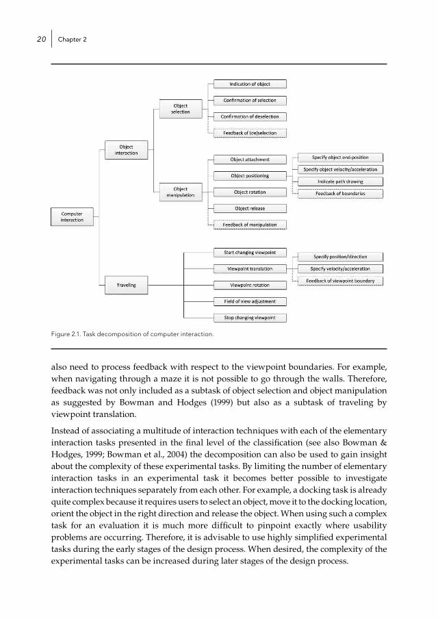
2.1.1 Task decompositionBased on the taxonomy of selection and manipulation techniques of Bowman and Hodges (1999) and the taxonomy of travel techniques of Bowman et al. (1999) we propose a slightly modified decomposition of computer interaction tasks (see Figure 2.1). In this task decomposition the selection/manipulation taxonomy is combined with the travel taxonomy to account for the most important 2D and 3D computer interaction tasks.
With respect to object interaction we made two modifications to the selection/manipulation taxonomy of Bowman and Hodges (1999). One of the adaptations is that we consider release as an inherent part of the selection task (i.e. object deselection) or the manipulation task (i.e. object release) and not as a separate subtask of object interaction. The other adaptation is that object positioning is further specified. Because object positioning can be viewed as an object travel task (an object is moved1 instead of the viewpoint) the elaboration of object positioning is adopted from the taxonomy of travel techniques (Bowman et al., 1999), i.e. the specification of the end-position and the velocity or acceleration. Furthermore, tasks are added to also be able to account for tasks like drawing (indicate path drawing) and tracing (feedback of boundaries).
With respect to travelling two subtasks were added to the taxonomy of travel techniques of Bowman et al. (1999). Navigation through a 3D environment cannot only be accomplished by translating and rotating the viewpoint, but also by changing the field of view (i.e. zooming). Therefore, field of view adjustment is added as a subtask of traveling. When adjusting the position of the viewpoint (viewpoint translation), users
1 Pointer movement is considered a special case of an object positioning task.
Chapter 220
also need to process feedback with respect to the viewpoint boundaries. For example, when navigating through a maze it is not possible to go through the walls. Therefore, feedback was not only included as a subtask of object selection and object manipulation as suggested by Bowman and Hodges (1999) but also as a subtask of traveling by viewpoint translation.
Instead of associating a multitude of interaction techniques with each of the elementary interaction tasks presented in the final level of the classification (see also Bowman & Hodges, 1999; Bowman et al., 2004) the decomposition can also be used to gain insight about the complexity of these experimental tasks. By limiting the number of elementary interaction tasks in an experimental task it becomes better possible to investigate interaction techniques separately from each other. For example, a docking task is already quite complex because it requires users to select an object, move it to the docking location, orient the object in the right direction and release the object. When using such a complex task for an evaluation it is much more difficult to pinpoint exactly where usability problems are occurring. Therefore, it is advisable to use highly simplified experimental tasks during the early stages of the design process. When desired, the complexity of the experimental tasks can be increased during later stages of the design process.
Figure 2.1. Task decomposition of computer interaction.
Interaction task design 21
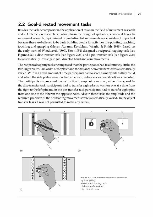
2.2 Goal-directed movement tasksBesides the task decomposition, the application of tasks in the field of movement research and 2D interaction research can also inform the design of spatial experimental tasks. In movement research, rapid-aimed or goal-directed movements are considered important because these are believed to be basic building blocks for activities like pointing, reaching, touching and grasping (Meyer, Abrams, Kornblum, Wright, & Smith, 1988). Based on the early work of Woodworth (1899), Fitts (1954) designed a reciprocal tapping task (see Figure 2.2a), a disc-transfer task (see Figure 2.2b) and a pin-transfer task (see Figure 2.2c) to systematically investigate goal-directed hand and arm movements.
The reciprocal tapping task encompassed that the participants had to alternately strike the two target plates. The width of the plates and the distance between them were systematically varied. Within a given amount of time participants had to score as many hits as they could and when the side plates were touched an error (undershoot or overshoot) was recorded. The participants also received the instruction to emphasize accuracy rather than speed. In the disc-transfer task participants had to transfer eight plastic washers one at a time from the right to the left pin and in the pin-transfer task participants had to transfer eight pins from one side to the other in the opposite holes. Also in these tasks the amplitude and the required precision of the positioning movements were systematically varied. In the object transfer tasks it was not permitted to make any errors.
(a) (b)
(c)
Figure 2.2. Goal-directed movement tasks used by Fitts’ (1954): a) reciprocal tapping task, b) disc-transfer task and c) pin-transfer task.
Chapter 222
The experimental tasks Fitts (1954) used are simple object interaction tasks intended to elicit goal-directed movements. When considering the task decomposition presented in the previous sections the tapping task consists of an object positioning task of an interaction device followed by an object selection task by means of physical touch, which is repeated a number of times. The disc-transfer task and the pin transfer task are straight-forward object manipulation tasks: an object attachment is followed by an object positioning task (traveling and final positioning) and an object release task after which the cycle is repeated until the remaining objects are re-positioned. This shows that in these interaction tasks a limited number of elementary interaction tasks are combined, which results in fairly simple, but representative experimental tasks. Consequently, 3D computer interaction tasks resembling these interaction tasks with real objects will be very useful in the systematic evaluation of 3D interaction techniques and input devices.
2.2.1 Pointing tasksIn the field of 2D interaction research more effort has been invested in designing standardized tasks for the evaluation of interaction techniques and input devices than in the field of 3D interaction research. These standardized tasks are presented in the ISO standard (ISO 9241-9, 2000) as part of a method for evaluating the efficiency and effectiveness of existing and new input devices. The structure of these standardized tasks closely resembles that of the tasks Fitts (1954) proposed to investigate goal-directed movements of the arm and hand. Especially the one-directional pointing task is very similar to the reciprocal tapping task used by Fitts. In the one-directional pointing task two target rectangles of a certain width and with a certain distance between them are presented to a user on a computer screen. The user is required to point at the two target rectangles alternately by moving a cursor back and forth and to select the target when the cursor is above it. In addition to the one-directional pointing task, a multi-directional pointing task is described in the ISO standard. In this task the targets are presented on the circumference of a larger circle and the user is required to point and select the targets in consecutive order (see Figure 2.3a). The advantage of a multi-directional task is that it takes into account the difficulty associated with the direction of the movement.
Instead of a reciprocal selection task, researchers can also choose to use a discrete selection task. For example, Card et al. (1978) used a discrete multidirectional selection task instead of a reciprocal selection task to demonstrate that Fitts’ law can also be applied to these interaction movements. Since a discrete task has more similarities with everyday computer use we believe that in order to evaluate the performance of input devices and interaction techniques it is preferable to use a discrete selection task instead of a reciprocal selection task. Figure 2.3b shows a discrete multi-directional selection task we used in a study aimed at investigating goal-directed movements in more detail (see also Nieuwenhuizen, Aliakseyeu, & Martens, 2009a). Although the targets appeared in different directions relative to the starting point (red target), only one destination target was shown at the time (green target).

Interaction task design 23
(a) (b)
Figure 2.3. 2D selection tasks a) reciprocal multidirectional selection task (adopted from the ISO standard, and b) discrete multidirectional selection task (adopted from Nieuwenhuizen et al., 2009a).
The interaction tasks described in the ISO standard have inspired the design of many 2D pointing tasks which were used to systematically evaluate interaction techniques and input devices. Unfortunately, there is no such standard for the design of 3D pointing tasks. We agree with Raynal et al. (2013) and Teather and Stuerzlinger (2011) that a standard comparable to the ISO 9241-9 for the evaluation of 2D computer interactions would benefit the systematic evaluation of 3D interaction techniques and input devices. Fortunately, several researchers in the field of 3D interaction have recently put effort in designing 3D experimental tasks that resemble the 2D interaction tasks described in the ISO standard (Pino, Tzemis, Ioannou, & Kouroupetroglou, 2013; Raynal et al., 2013; Teather & Stuerzlinger, 2011).
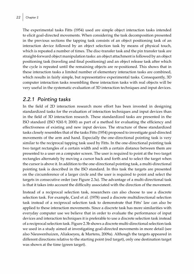
Teather and Stuerzlinger (2011) designed a 3D version of the 2D reciprocal multi-directional selection task in which thirteen spherical targets were placed on top of cylinders of varying height (see Figure 2.4a). Pino et al. (2013) diverged somewhat more from the multidirectional selection task in their design of a 3D selection task. They placed eight spheres on the vertices of a cube and the user had to select the target which was diagonally opposite from the starting target to which the cursor automatically teleported. Figure 2.4b shows an example of a 3D implementation of the 2D selection task we used in a previous study (see Figure 2.3b). This example resembles the discrete selection task Raynal et al. (2013) proposed in which the spherical targets were placed onto a larger supportive sphere. The task axis between the starting sphere and the destination sphere always ran through the center of the sphere.
We believe that this approach towards the design of simple but representative selection tasks allows for a systematic evaluation of 3D selection interactions. Besides the general
Chapter 224
layout of the 3D selection tasks there are various task parameters that should be considered when designing these interaction tasks. Besides the independent variables target size, target distance and target direction (which are also mentioned in the ISO standard) Poupyrev et al. (1997) presented several other task parameters that are important to take into account when designing 3D selection tasks:
- number of objects to be selected, - occlusion of target object, - presence and density of distractor objects, - dynamics of target object (e.g. moving or stationary), and - bounding volume of target object.
In addition to these task parameters there are still some other parameters to consider. For example, in the case of a multidirectional selection task or when distractor objects are present it should be clearly communicated what the destination target is. Furthermore, it should be determined whether or not visual or auditory cues will be provided in the case of a target selection or a target miss. Another consideration is what to do when a target is missed, i.e. will the trial be ended or will the participant be able to continue until the target is correctly selected. For a 3D environment it should also be considered to enhance depth perception (e.g. with head tracking and/or textured environments) for this will be beneficial for the user’s performance. Awareness of the possible task parameters, such as the ones mentioned above, is imperative when pursuing to design the most optimal 3D selection task for gathering the required interaction data.
(a) (b)
Figure 2.4. 3D selection tasks: a) reciprocal multidirectional selection task (adopted from Teather and Stuerzlinger, 2011), and b) example of a 3D discrete multi-directional selection task derived from the 2D discrete selection task in Figure 2.3b (starting sphere lies in the center of the surrounding target spheres).
Interaction task design 25
2.2.2 Tracing tasksOther goal-directed movements that have been extensively studied are strokes, i.e. the fundamental units of human handwriting movements (Plamondon, 1993). Pencil strokes were studied already in 1899 by Woodworth to determine the relationship between speed and accuracy of voluntary upper limb movements (Woodworth, 1899). Participants were required to make horizontal pencil strokes at a constant speed on a paper attached to a kymograph, rotating on a horizontal axis. Plamondon and others investigated handwriting strokes in detail and were able to model goal-directed strokes for signature verification and handwriting recognition (Plamondon & Clément, 1991; Plamondon & Guerfali, 1998; Plamondon, Yu, Stelmach, & Clement, 1991). The task they used required participants to draw 2 cm lines on a paper grid with a digitizer pen, while the direction of the movement was specified on a display.
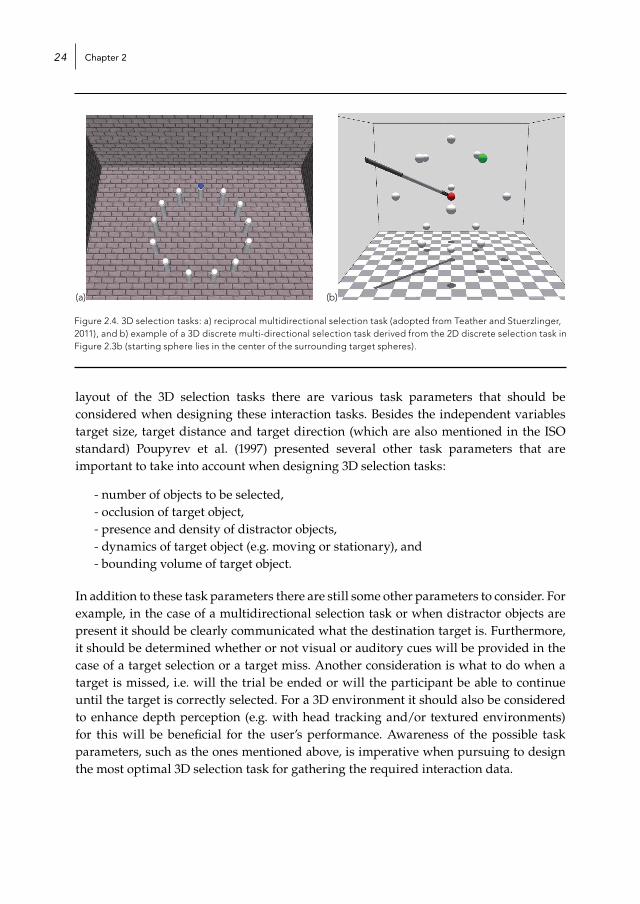
The development of the pen computing technology facilitated writing and drawing on a computer. As a result, trajectory-based tasks such as writing and drawing are nowadays also common computer interaction tasks (Accot & Zhai, 1999). The ISO standard (ISO 9241-9, 2000) includes two trajectory-based tasks to systematically investigate these tracing movements, as well as steering movements (e.g. steering through nested menus). The general layout of the one-directional straight tracing task is very similar to that of the one-directional selection task. In this one-directional tracing task participants are required to move an object (or draw a line) from one side of a straight tunnel (i.e. two parallel lines) to the other. The width and the length of the tunnel can be systematically varied.
(a) (b)
Figure 2.5. 2D tracing tasks: a) round tracing task (adopted from ISO standard), and b) multidirectional straight tracing task (adopted from Nieuwenhuizen et al., 2009a).
Chapter 226
The other trajectory-based task in the ISO standard is a circular (any direction) tracing task (see Figure 2.5a) in which the participant moves an object (or draws a line) through a circular tunnel with a certain width and radius. Although this task is presented as an any direction tracing task the movement is fundamentally different from a straight tracing task positioned in various different directions. Figure 2.5b shows an implementation of a multidirectional straight tracing task we used in a study aimed at investigating goal-directed movements in more detail (see also Nieuwenhuizen et al., 2009a). As in the case of the selection tasks, the layouts of these 2D tracing tasks are quite simple and the difficulty of the task (i.e. length, width and direction of the paths) can be systematically varied.
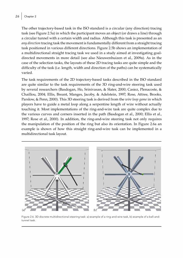
The task requirements of the 2D trajectory-based tasks described in the ISO standard are quite similar to the task requirements of the 3D ring-and-wire steering task used by several researchers (Basdogan, Ho, Srinivasan, & Slater, 2000; Casiez, Plenacoste, & Chaillou, 2004; Ellis, Breant, Manges, Jacoby, & Adelstein, 1997; Rose, Attree, Brooks, Parslow, & Penn, 2000). This 3D steering task is derived from the wire loop game in which players have to guide a metal loop along a serpentine length of wire without actually touching it. Most implementations of the ring-and-wire task are quite complex due to the various curves and corners inserted in the path (Basdogan et al., 2000; Ellis et al., 1997; Rose et al., 2000). In addition, the ring-and-wire steering task not only requires the manipulation of the position of the ring but also its orientation. In Figure 2.6a an example is shown of how this straight ring-and-wire task can be implemented in a multidirectional task layout.
(a) (b)
Figure 2.6. 3D discrete multidirectional steering task: a) example of a ring-and-wire task, b) example of a ball-and-tunnel task.
Interaction task design 27
Casiez et al. (2004), used straight paths because they believed that complicated paths would not allow them to distinguish between the influence of different input devices and the influence of learning time. In addition, they implemented the ring-and-wire task in such a way that the cursor orientation was automatically oriented perpendicular to the path. This reduces the complexity of the task since participants only have to focus on the positioning of the ring and not its orientation. However, this automatic orientation of the cursor cannot be implemented when there are sharp bends in the path. Therefore, the ball-and-tunnel task Casiez et al. (2004) also used in their experiment lends itself somewhat better for a straightforward steering or position manipulation task. Liu, Martens and van Liere (2011a) also designed a ball-and-tunnel task to decouple the positioning of the input device from the orientation of the input device. In this task the target ball in the tunnel is pushed forward with a cursor ball. The use of a spherical shape for both the target and the cursor ensured that they intersected at one point and that the orientation of the input device did not play a role during the steering task. Figure 2.6b shows an example of how the straight ball-and-tunnel task can be implemented in a multidirectional task layout.
Also in the case of the 3D trajectory-based tasks, such as the ones described above, there are several task parameters that should be taken into account when designing these tasks. In the ISO standard some independent variables are mentioned, such as path length (or radius of the circular path), path width and path direction. Other task parameters that can be varied are:
- number of curves in path, - curvature of bend(s) in path, - occlusion of path, - texture of tunnel, and - size of target object within tunnel.
Furthermore, it should be determined what to do when the steering movement is out of bounds, i.e. does the participant have to restart at the beginning or is the participant able to continue where he/she left off. In addition, it would help the participant if it is clearly communicated when the steering movement is out of bounds (e.g. by means of visual or auditory feedback). As in the case of the selection task, the enhancement of depth perception (e.g. with head tracking and/or textured environments) will also benefit the performance.
The designs of the 3D selection and tracing tasks described in this section are highly straightforward, which is also indicated by the limited number of elementary interaction tasks that are incorporated in these tasks. Nevertheless, these tasks are still representative in that they are able to elicit goal-directed movements, which are the basic building blocks for numerous computer interactions. Therefore, we believe that these 3D selection and tracing tasks are highly suitable for formative usability testing to iteratively and quantifiably assess and improve an interaction design. In other words, these 3D interaction tasks, together with the task decomposition, provide

Chapter 228
a solid base for the development of tasks to systematically evaluate selection and steering movements.
2.3 experimental set-upFor the development of a more thorough analysis method to assess the quality of interaction movements we used datasets of a 2D discrete multidirectional selection task, a 2D multidirectional straight tracing task and a 3D ball-and-tunnel steering task. The 2D datasets are used for the data analysis of Chapter 3, 4 and 5 and the 3D dataset is analyzed in Chapter 6. The method of the 2D selection and tracing experiment is described in Section 2.3.1 (see also Nieuwenhuizen et al., 2009a) and the method of the 3D steering experiment is described in Section 2.3.2 (see also Liu, van Liere, & Kruszyński, 2011b)2.
2.3.1 Method 2D interaction
2.3.1.1 ParticipantsEight university employees voluntarily participated in a typical Fitts’ law study that we undertook to generate data that we intended to use to explore the characteristics of simple interaction movements. The group consisted of 5 males and 3 females. Their age ranged from 30 to 35 years (M = 32.4 years). All participants indicated that their right hand was their preferred hand when using the mouse. Two participants indicated that their left hand was the preferred hand when using the stylus.
2.3.1.2 Experimental TaskParticipants were asked to perform a multi-directional point-and-select task and a multi-directional tracing task:
Point-and-select task: Participants were required to select a presented target as fast as possible but they were asked not to miss too many targets. In this task 8 target circles were arranged in larger circles with a diameter of 48 mm, 96 mm and 144 mm around a central home circle (see Figure 2.7a). The targets had three different sizes: 3 mm, 6 mm and 9 mm. The 9 combinations of target distance (A) and target size (S) resulted in 7 different levels of difficulty (ID= 2.7, 3.2, 3.5, 4.1, 4.6, 5 and 5.6 bits3). At the beginning of a new trial, the target was presented together with the home circle (3 mm). The targets were presented in random order, with the restriction that subsequent targets were never positioned in the same direction. The data collection started when the home circle was selected and continued until the target was correctly selected.
2 Both experiments were conducted within the QUASID research project, which was a cooperation between the Eindhoven University of Technology and the Centrum voor Wiskunde en Informatica (CWI) in Amsterdam funded by the Nederlandse Organisatie voor Wetenschappelijk Onderzoek (NWO). Due to this cooperation, researchers were granted access to each other’s data.
3 ID is the index of difficulty in “bits/response”: log2(2A/W), see also Chapter 3.
Interaction task design 29
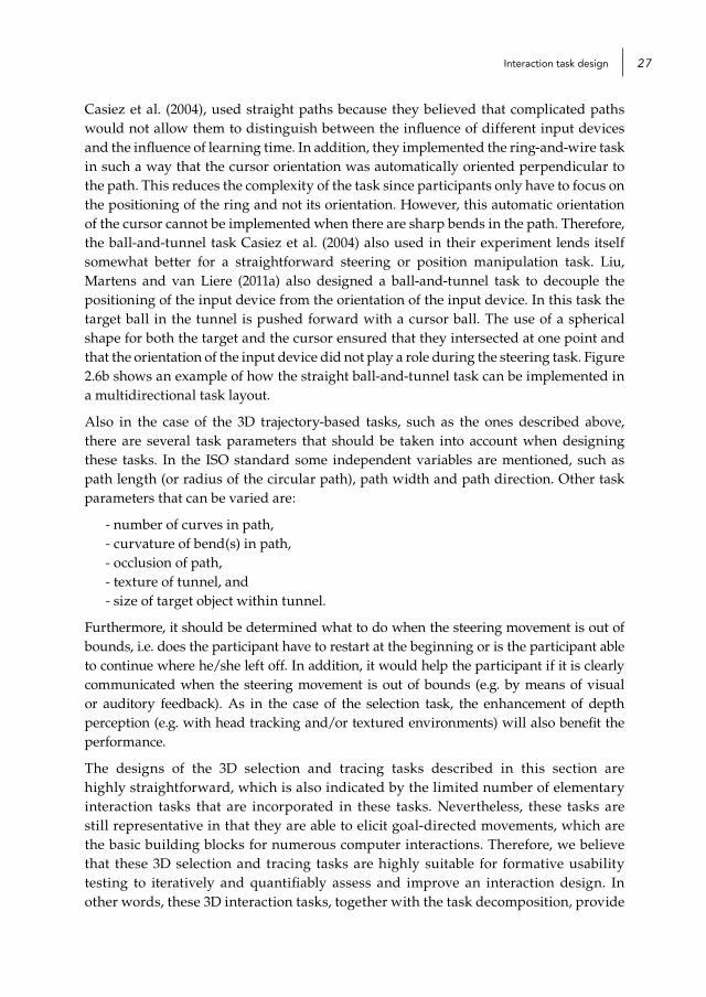
Tracing task: Participants were required to make tracing movements through a straight tunnel as fast as possible. In this task tunnels of 3 different lengths (48 mm, 96 mm and 144 mm) were positioned in 8 different directions (see Figure 2.7b). The tunnels were of 3 different widths: 7 mm, 14 mm and 21 mm. The start area was 3 mm in length, whereas the stop area was 10 mm in length. The 9 combinations of tunnel length (L) and tunnel width (W) resulted in 7 different levels of difficulty (ID = 2.29, 3.43, 4.57, 6.86, 10.29, 13.71, 20.57 bits). At the beginning of a trial only one tunnel was presented. The tunnels were presented in random order, with the restriction that subsequent tunnels were never positioned in the same direction in order to prevent learning effects. The data collection started when a button press occurred while the cursor was on top of the start area and continued until the button was released while the cursor was on top of the stop area. When the button was released while the cursor was not on top of the stop area or when the cursor did not stay within the tunnel boundaries the trial would be restarted. Although these trials were recorded they are not included in the analysis of movement paths.
(a) (b)
Figure 2.7. Experimental task: a) point-and-select task; b) tracing task.
2.3.1.3 ApparatusThe selection task was presented on a 21-inch WACOM Cintiq 21UX tablet, with integrated display. The resolution of the screen was set at 1600x1200 pixels. The position of the screen was changed in between sessions: when participants were using the mouse the screen was positioned vertically and when they were using the stylus the screen was tilted horizontally so that the screen would face upwards (see Figure 2.8). The mouse had a constant CD-ratio of 1:4, while the CD-ratio was obviously equal to 1:1 in the case of the stylus with integrated display.

Chapter 230
(a) (b)
Figure 2.8. Screen set-up: a) when using the mouse; b) when using the stylus.
2.3.1.4 DesignThe design of the experiment followed a 2x2x3x3x8 within-subjects model with task (2 levels), input device (2 levels), target distance ‘A’ or tunnel length ‘L’ (3 levels), target size ‘S’ or tunnel width ‘W’ (3 levels) and 8 directions as independent variables. The eight directions will be condensed into 2 levels, namely orientation (horizontal-vertical versus oblique). This resulted for each task in a 2x3x3x2 within-subjects model.
2.3.1.5 ProcedureAt the beginning of the experiment session a short instruction about the task was presented on the WACOM display. The experiment consisted of 4 (2 task x 2 input device) sessions, each containing 72 trials, i.e., 8 target directions combined with 3 different sizes and 3 different distances. A practice session of 27 trials, i.e., 3 directions combined with 3 sizes and 3 distances, preceded each actual experimental session. During these practice trials participants could adjust to a change in condition. The order of the four experimental sessions was balanced so that the number of participants using the mouse during the first session was equal to the number of participants using it during the second session. In addition, the number of participants performing the selection task during the first session was equal to the number of participants performing this task during the second session.
2.3.2 Method 3D interaction
2.3.2.1 ParticipantsFourteen right-handed computer users voluntarily participated in the 3D steering experiment. Of these 14 participants 10 had previous experience of working with virtual environments. The group consisted of 11 males and 3 females and their age ranged from 25 to 38 years (M = 32.3).
Interaction task design 31
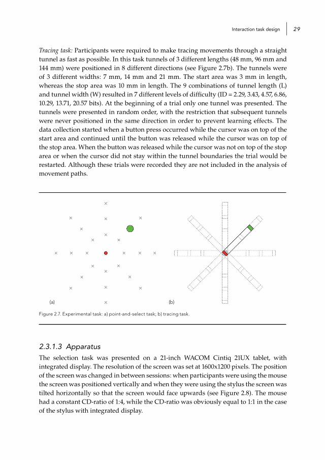
2.3.2.2 Experimental taskThe ball-and-tunnel task required users to push a virtual target ball through a tunnel, with the same diameter as the target ball, as fast as possible. The interaction device was an input stylus with a small cursor ball (with a radius of 5 mm) on the tip of the stylus. This cursor ball was used to enlarge the interaction area between the stylus and the target ball, since it is easier to push the target ball with a volume than with a point. The use of a spherical shape for both the target and the cursor ensures that they intersect at one point and that the orientation of the input device does not play a role during the steering task. When the cursor ball was in contact with the target ball, the target ball could be pushed through the tunnel. Consequently, the steering path width (the amplitude of the cursor ball when in contact with the target ball) is larger than the tunnel width, namely the tunnel width plus two times cursor ball radius (see Figure 2.9a). When the cursor ball lost contact with the target ball and the cursor ball did not intersect with the tunnel, the user had to return the cursor ball to the tunnel and continue the task from where he/she left off. This means that the position of the target ball can be used as a progress indicator of the task.
In this experiment force feedback is used to support the participants’ task performance. The aim of the force feedback is to assist the participants, to some extent, in keeping the cursor ball within the path boundaries. In practice, participants feel as if the cursor ball is dragged slightly toward the center of the tunnel once they deviate from the center of the tunnel (but are still within the tunnel). The magnitude of the force (F) is proportional to the distance that the cursor ball deviates from the center of the tunnel (see Figure 2.9b) and is computed by Hooke’s law:
F = kD , (2.1)
where k resembles a spring constant (k = 50 N/m) and D is the distance (D ∈ [0, radius tunnel]). The direction of the force is from the center of the cursor ball to the nearest point on the tunnel center (see Figure 2.9b).
(a) (b)
Figure 2.9. Ball-and-tunnel task: a) a cursor ball pushes a target ball through a tunnel. Tunnel width = diameter of target ball; steering path width = tunnel width + 2x radius cursor ball = 2x (radius of target ball + radius of cursor ball), b) task with force feedback in which any deviation from the tunnel center is pulled back by a force that is proportional to the distance of the deviation.

Chapter 232
The tunnels were of 3 different lengths (240 mm, 300 mm and 360 mm) and of 2 different widths (20 mm and 30 mm4). The combinations of tunnel length (L) and steering path width (W) resulted in 6 different levels of difficulty (ID = 6, 7.5, 8, 9, 10, 12). Furthermore, paths of different curvatures were used, where curvature is defined as ρ = 1/radius. In this way, a path can be thought of as a segment on a circle with a given radius. The four curvature values corresponded to a circle with an infinite radius (straight line) and with a radius of 250 mm, 125 mm and 83.3 mm (see Figure 2.10). The paths were positioned in the xy-plane with the start of the paths at the origin. The trial started when the target ball was at the beginning of the tunnel and the task continued until the target ball reached the end of the tunnel.
Figure 2.10. Four different path curvatures.
2.3.2.3 ApparatusThe experiment was performed in a desktop virtual environment (see Figure 2.11a), equipped with:
- desktop PC with an Intel (R) Core (TM) 2 Quad CPU Q6600 (2.40 GHz) and a Nvidia Quadro FX 5600 GPU,
- 67-inch 3D-capable Samsung HL67A750 LED DLP HDTV, - pair of NuVision 60GX stereoscopic LCD glasses, - ultrasound Logitech 3D tracker, and - Novint Flacon haptic device (see Figure 2.11b).
4 The tunnel widths of 20mm and 30mm correspond to steering path widths of 30mm and 40mm, respectively (tunnel width plus two times cursor ball radius of 5mm).

Interaction task design 33
(a) (b)
Figure 2.11. Experimental set-up: a) desktop VR environment, and b) the Novint Falcon haptic device.
The monitor resolution was set at 1920 x 1080 pixels. The monitor had a refresh rate of 120 Hz, the Falcon was updated around 700 Hz5 and the head tracker had a refresh rate of 60 HZ. The overall end-to-end latency of the system during the experiment was measured to be approximately 80 ms, using the method proposed by Steed (2008).
2.3.2.4 DesignWe adopted a repeated measures design in each block, introducing paths of different length, width and curvature. The specific settings for each property include:
- path length (L): 0.24 m, 0.30 m, 0.36 m - path width (W): .03 and .04 m - path curvature (ρ): 0, 4, 8, and 12 m-1 - force feedback: on and off.
Each condition (a combination of path properties and force feedback) was repeated 3 times, resulting in 3x2x4x2x3 trials (L x W x ρ x F x repetition) per participant. There were in total 2016 trials for 14 participants.
2.3.2.5 ProcedureThe experiment consisted of two sessions: with force feedback and without force feedback. The order of these two experimental sessions was balanced, which means that half of the participants started with the session in which the force feedback was turned on and the other half started with the session in which the force feedback was turned
5 Our sense of touch is far more sensitive than our visual system. In graphics a refresh rate of 60Hz is quite acceptable, while in haptics it is widely believed that a response frequency of 300-1000Hz is needed to ensure accurate interaction (Delingette, 1998; Picinbono, Lombardo, Delingette, & Ayache, 2002). Although, the Falcon is able to update at 1000Hz, the frequency was reduced to approximately 700Hz due to other computational requirements (e.g. scene rendering). Nevertheless, this still managed to provide a consistent and smooth sense of touch.

Chapter 234
off. Participants were required to practice an equal number of trials at the beginning of each session before the data collection was started. Trials were presented in a random order which differed from one participant to another. Participants were allowed to have a break whenever they suffered from fatigue between trials.

Chapter 3
Performance characterization: Fitts’ law
Chapter 336
3.1 task performance characterizationAs mentioned in the previous chapter, research with respect to 2D interaction has invested effort in designing standardized tasks, such as selection and tracing tasks. The difficulty of these tasks can be varied, for example, by using distinct target distances or tunnel lengths and by varying target sizes or tunnel widths. Although participants are asked to emphasize accuracy rather than speed when executing the tasks of varying difficulty, there is an intuitive trade-off between speed and accuracy. When participants are moving fast they are more prone to make errors and when participants pursue accuracy they will move slower in order not to make mistakes. This speed-accuracy relationship is frequently used to describe task performance and is best known as Fitts’ law (Fitts, 1954).
3.1.1 Speed-accuracy trade-off: Fitts’ lawFitts (1954) modeled the speed-accuracy relationship by relating the time required to rapidly move to a target area to the target distance and the target size. Fitts’ law was originally developed to model human movement on a one-dimensional repetitive tapping task. Card et al. (1978) were the first to also use Fitts’ law to compare the performance of various input devices, such as a mouse, a rate-controlled isometric joystick, step keys, and text keys. Over the years, Fitts’ law has been frequently applied and as a result it has become a well-established model in the HCI field.
The Fitts’ law model originates from information theory and is based on the assumption that performance is limited by the information capacity of the motor system. According to Fitts (1954) “the information capacity of the motor system is specified by its ability to produce consistently one class of movements from among several alternative movement classes”. It becomes more difficult to produce the same motor response when the distance towards the target increases or when the target width, or tolerance limit, decreases. To compare performance across conditions Fitts defined the index of performance (Ip) as:
Ip = -log2(Ws/2A)/t bits/sec , (3.1)
where t is the average movement time, Ws is the target width and A is the amplitude or target distance. The logarithmic term is called the index of difficulty (ID) in ‘bits/response’, which increases with a larger target distance and a smaller target width. The index of performance was initially intended to compare different task conditions with each other and Fitts (1954) was able to show that it was approximately constant over a range of target distances and target widths.
3.1.2 Issues with respect to Fitts’ lawAlthough Fitts’ law has been frequently used as a performance model, we can identify several issues that should be more thoroughly addressed in order to draw methodologically sound conclusions from the Fitts’ law comparison method.
Performance characterization: Fitts’ law 37
3.1.2.1 Issue 1: Applying parametric statisticsFitts and Peterson (1964) used the index of performance to describe movement time as a function of the ratio between target distance and target width:
T = a + b ID = a + b log2 (2A/Ws), (3.2)
where a and b are linear regression coefficients and ID is the index of difficulty. This relationship was not only used to compare different task conditions with each other but also to characterize different experimental conditions by means of their regression coefficients (Fitts & Peterson, 1964; Fitts & Radford, 1966). For example, Fitts and Peterson (1964) compared two different experimental tasks (continuous vs. discrete movement) and Fitts and Radford (1966) compared different instruction conditions (accurate vs. fast) and movement-preparation conditions (self-initiated responses vs. responses initiated following a signal). This trend of comparing not only the task conditions but also other experimental conditions was adopted by several researchers in the HCI field, who mainly use Fitts’ law to compare input devices or interaction techniques with each other (Balakrishnan, 2004; Card et al., 1978; Guiard, Beaudouin-Lafon, & Mottet, 1999; Isokoski, 2006; MacKenzie, Sellen, & Buxton, 1991).
When comparing averages or when performing other parametric statistical analyses, such as linear regression, it is essential that the data distributions around the different mean values are normal with equal variances (i.e. satisfy homoscedasticity). When this condition is not satisfied, then drawing conclusions about the magnitude of differences (i.e. the effect sizes) between conditions using standard methods such as a t-test is, strictly speaking, not allowed (Grissom & Kim, 2005). Especially the normality assumption poses a problem for the Fitts’ law analysis method as response time distributions are frequently positively skewed: the longest response times are usually much longer than the average response time whereas the shortest response times are rarely much smaller than the average response time (Heathcote, Popiel, & Mewhort, 1991). In addition, the standard deviation of the measured times usually increases with the average task completion time. This means that the task completion times of easy tasks, which generally take less time than more difficult tasks, show less variation than the task completion times of more difficult tasks.
It is possible to correct for problems with normality and homoscedasticity of distributions by transforming the data (Field, 2009). A common way of dealing with the positively-skewed time distributions is to take the logarithm of time, i.e. applying a logarithmic transformation. However, a clear motivation for this logarithmic transformation over other non-linear transformations seems to be missing. It is suggested by Field (2009) to just try out different transformations and observe the effect on the equality of variance. We will propose an alternative approach to this problem that is more theoretically sound.

Chapter 338
3.1.2.2. Issue 2: Calculating average values over participantsIn general, mean values are calculated for each experimental condition before regression analysis is applied to the movement times in order to determine the Fitts’ law regression coefficients. Determining the mean value for each experimental condition, amongst others, implies that the differences between participants are not taken into account. In other words, the data is being treated as between-subjects data instead of within-subjects data.
Fitts and Radford (1966) presented the results of their tapping task study for each participant separately. Their results illustrated that there were considerable differences between participants with respect to both regression coefficients, which indicated that people were comfortable with different speed-accuracy trade-offs. This means that a part of the variation in the data can be explained by the differences between people, hence masking within-subject effects. Therefore, we propose that when modeling time performance data according to Fitts’ law, the model should also offer the possibility to account for differences in speed-accuracy trade-offs between participants.
3.1.2.3 Issue 3: Judging lack of fitAnother important issue is the possibility to judge whether or not the proposed linear regression model fits the data well. A lack-of-fit (LOF) test is traditionally used to determine a model’s fit (Draper & Smith, 1998):
,(3.3)
where Yij are the individual observations, i is the average of response values (y-values) for one specific predictor value (x-value), i and ni are the corresponding predicted response value and number of repetitions, n is the number of distinct predictor values and N is the total number of observations. As indicated by Equation (3.3) the lack-of-fit test includes two parts: a lack-of-fit sum of squares in the nominator that can possibly be reduced by increasing the complexity of the model used to predict the averages, and a residual sum of squares in the denominator that is not influenced by this prediction. The lack-of-fit test allows to assess (by means of an F(n-2, N-n) test) the discrepancy between the observed averages and the ones predicted by the model.
Equation (3.3) reveals that the lack of fit can only be determined when each experimental condition contains multiple observations. In other words, there should be more than one value of the response variable for each value of the predictor variable (Kleinbaum, Kupper, Nizam, & Muller, 2007). However, as mentioned in the previous section, mean values for the experimental conditions are often calculated first before applying Fitts’ law. This means that the variation present in the data is discarded, which removes the possibility to judge the accurateness or the ‘fit’ of the model.

Performance characterization: Fitts’ law 39
Instead of using the lack-of-fit test to judge the model’s fit researchers provide the R-squared1 and argue that the data fits well when it is close to one (Drewes, 2010). When there is only a limited amount of data points (for instance, by only modeling the mean values) it is relatively easy to get an R-squared close to one. There are hence two problems with using R-squared to judge the lack of fit. First, R-squared is a measure of effect size and, therefore, it is not really an accepted criterion for expressing the lack of fit of a (linear) model. Second, there is no accepted method to specify a threshold value for R-squared in order to distinguish models with an adequate fit from others.
3.1.2.4 Issue 4: Using effective width instead of target widthIn order to correct for the varying error rates at different ID values the effective target width (We) is frequently used in Fitts’ law calculations instead of the displayed target width (W):
We = 4.133 · SDx, (3.4)
where SDx is the standard deviation of the selection coordinates measured along the task axis (ISO 9241-9, 2000). The coefficient in Equation (3.4) corresponds to a nominal error rate of 4%, which means that 96% of the end-point distribution is covered (MacKenzie, 1992; Murata, 1999).
The effective target width is not a priori known, but can only be calculated after the data is collected and as such becomes a measured quantity. One of the assumptions of linear regression analysis is that an independent variable is assumed to be error-free, which means that it should not be contaminated with measurement errors (Poole & O’Farrell, 1971). Because the effective width is a measured quantity (containing measurement error), it is advised to use statistical methods that can deal with two measured quantities, such as structural equation modeling (SEM) or multidimensional scaling (MDS), instead of linear regression analysis (i.e. Fitts’ law). Consequently, we prefer not to use the effective target width and to optimize the data fit in a different way.
Another reason for using the nominal target width (W) instead of the effective target width (We) was put forward by Zhai, Kong and Ren (2004). They systematically explored the speed-accuracy tradeoff based on the a priori known target width (W) and the a posteriori determined effective target width (We). One of the conclusions was that “Revisions of index difficulty to a behavior form, either through We, or its more aggressive version Wm, consistently weaken the regularity within a particular operating bias condition”. In other words, the goodness of fit within each condition was reduced when using We instead of W, which is not desirable when comparing conditions within the experiment.
1 R-squared is the proportion of variability in a data set that is accounted for by the statistical model.

Chapter 340
3.1.2.5 Issue 5: Variations of Fitts’ lawThe number of variations to Fitts’ law that have been proposed over the years is another issue. As Fitts’ law is sometimes used to compare the results of different experiments with each other it becomes particularly difficult when researchers apply different formulations of Fitts’ law. Welford (1968) was the first to propose an alternative formulation, which, in his opinion, was based on an improved index of task difficulty:
T = a + b · log2(A/W + 0.5) (3.5)
MacKenzie (1989) proposed yet another adjustment to the Fitts’ law formula based on Shannon’s Theorem 17 which to his opinion was “more theoretically sound” and would yield “a better fit with empirical data” (see also MacKenzie et al., 1991):
T = a + b · log2(A/W + 1) (3.6)
The above-mentioned variations of the Fitts’ law formula do not question the logarithmic relationship between movement time and the task characteristic (i.e. the ratio between target distance and target width). Meyer et al. (1988) however argue, based on a statistical model of movement performance, that the relationship should not be logarithmic but square root:
T = a + b · (A/W)0.5 (3.7)
In turn, according to Accot and Zhai (1999) this relationship should be a linear one when considering steering movements through a straight tunnel:
T = a + b · (A/W), (3.8)
where a and b are regression coefficients, A is the length of the tunnel and W is its width.
These variations in Fitts’ law show that there is no consensus about the precise relationship between movement time and the task characteristic (A/W). This lack of consensus, combined with the finding that people might adhere to different speed-accuracy trade-offs, warrants for a more general approach towards Fitts’ law modeling.
In order to deal with the issues described above we propose a slightly more general model, i.e. a power-law model, which includes all previous proposals of Fitts’ law as special cases.
3.1.3 Data processing and statistical modelingIn this section we propose the use of non-linear power-law models for two purposes. The first purpose is to characterize the relationship between average task completion times and task characteristic (A/W). Using this class of models it is possible to investigate what kind of relationship, e.g. linear, logarithmic, square root or other, can best express this mapping for a specific data set. Second, the power-law modeling approach also makes it possible to correct for problems with normality and homoscedasticity of the data and
Performance characterization: Fitts’ law 41
with differences between participants. The method of maximum-likelihood estimation (MLE) will be used throughout to estimate and compare the parameters of our non-linear models. According to this method the optimum estimate of model parameters is obtained by maximizing the likelihood function (Martens, 2009). This MLE takes all the data into account and not merely the mean values when assessing the lack of fit between a model and the data and is, moreover, not restricted to linear (regression) models.
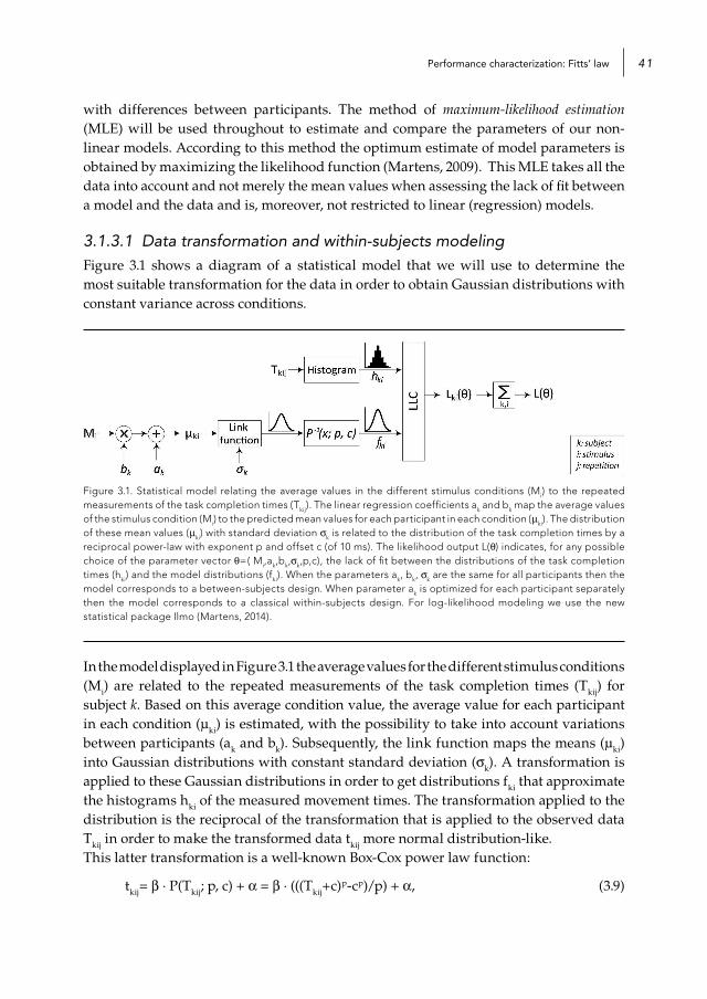
3.1.3.1 Data transformation and within-subjects modelingFigure 3.1 shows a diagram of a statistical model that we will use to determine the most suitable transformation for the data in order to obtain Gaussian distributions with constant variance across conditions.
Figure 3.1. Statistical model relating the average values in the different stimulus conditions (Mi) to the repeated measurements of the task completion times (Tkij). The linear regression coefficients ak and bk map the average values of the stimulus condition (Mi) to the predicted mean values for each participant in each condition (µki). The distribution of these mean values (µki) with standard deviation σk is related to the distribution of the task completion times by a reciprocal power-law with exponent p and offset c (of 10 ms). The likelihood output L(θ) indicates, for any possible choice of the parameter vector θ=( Mi,ak,bk,σk,p,c), the lack of fit between the distributions of the task completion times (hki) and the model distributions (fki). When the parameters ak, bk, σk are the same for all participants then the model corresponds to a between-subjects design. When parameter ak is optimized for each participant separately then the model corresponds to a classical within-subjects design. For log-likelihood modeling we use the new statistical package Ilmo (Martens, 2014).
In the model displayed in Figure 3.1 the average values for the different stimulus conditions (Mi) are related to the repeated measurements of the task completion times (Tkij) for subject k. Based on this average condition value, the average value for each participant in each condition (µki) is estimated, with the possibility to take into account variations between participants (ak and bk). Subsequently, the link function maps the means (µki) into Gaussian distributions with constant standard deviation (σk). A transformation is applied to these Gaussian distributions in order to get distributions fki that approximate the histograms hki of the measured movement times. The transformation applied to the distribution is the reciprocal of the transformation that is applied to the observed data Tkij in order to make the transformed data tkij more normal distribution-like. This latter transformation is a well-known Box-Cox power law function:
tkij= β · P(Tkij; p, c) + α = β · (((Tkij+c)p-cp)/p) + α, (3.9)
Chapter 342
where tkij are the transformed task completion times and (α, β) are usually chosen such that the minimum and maximum data values are mapped onto themselves (see Martens, 2003).
The statistical model in Figure 3.1 enables the optimization of the Box-Cox transformation instead of assuming that a specific transformation on the data (e.g. logarithmic) is the best solution. The maximum likelihood criterion L(θ) expresses the lack of fit, for any possible choice of parameters, between the modeled distributions (fki) and the observed distributions of the task completion times (hki). By keeping the value of σk constant across the different experimental conditions, we explicitly pursue that the transformed data satisfy as closely as possible the requirement of homoscedasticity. When applying a transformation to data, this transformation can obviously not depend on the conditions that need to be compared with each other (Field, 2009), which is why the parameters (p and c) of this transformation are independent of such conditions. It is relatively straightforward to adapt the model of Figure 3.1 to a within-subjects design by determining the likelihood for each participant separately and summing them to obtain the overall likelihood. The model in Figure 3.1 corresponds to a within-subjects design when the parameters ak, bk, and σk are optimized separately for each participant k. This can be viewed as a within-subjects correction. When b1=…=bk and σ1=…=σk, then the within-subjects correction corresponds to the correction proposed by Loftus and Mason (1994). The measured times after transformation and within-subjects corrections can be used in parametric analysis methods such as factor analysis and multi-dimensional scaling.
3.1.3.2 Modeling Fitts’ lawIn Figure 3.2 we present Fitts’ law as a statistical model. The difference between this model and the model shown in Figure 3.1 is that the average values for each participant in each condition (µki) are derived from the independent variable task characteristic (Ai/Wi).
Figure 3.2. Power-law model relating Ai/Wi in condition i to the repeated measurements of the task completion times (Tkij). The linear regression coefficients ak and bk map the index of difficulty IDi
*, which is a power-law function of Ai/Wi with exponent q and offset d, to the predicted average response time µki
*. The likelihood output L(θ) indicates, for any possible choice of the parameter vector θ=( ak,bk,µki,σk,p,c), how well the difference between the distributions of the task completion time (hki) and distributions of the mean values (fki) can be described by a Gaussian distribution with standard deviation equal to σk. When parameters ak, bk, σk are the same for all participants the model corresponds to a between-subjects design. When parameter bk is optimized for each participant separately the model corresponds to a classical within-subjects design.
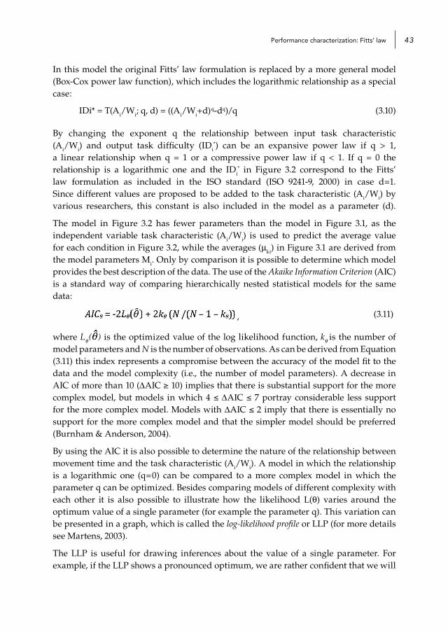
Performance characterization: Fitts’ law 43
In this model the original Fitts’ law formulation is replaced by a more general model (Box-Cox power law function), which includes the logarithmic relationship as a special case:
IDi* = T(Ai/Wi; q, d) = ((Ai/Wi+d)q-dq)/q (3.10)
By changing the exponent q the relationship between input task characteristic (Ai/Wi) and output task difficulty (IDi
*) can be an expansive power law if q > 1, a linear relationship when q = 1 or a compressive power law if q < 1. If q = 0 the relationship is a logarithmic one and the IDi
* in Figure 3.2 correspond to the Fitts’ law formulation as included in the ISO standard (ISO 9241-9, 2000) in case d=1. Since different values are proposed to be added to the task characteristic (Ai/Wi) by various researchers, this constant is also included in the model as a parameter (d).
The model in Figure 3.2 has fewer parameters than the model in Figure 3.1, as the independent variable task characteristic (Ai/Wi) is used to predict the average value for each condition in Figure 3.2, while the averages (µki) in Figure 3.1 are derived from the model parameters Mi. Only by comparison it is possible to determine which model provides the best description of the data. The use of the Akaike Information Criterion (AIC) is a standard way of comparing hierarchically nested statistical models for the same data:
, (3.11)
where Lθ( ) is the optimized value of the log likelihood function, kθ is the number of model parameters and N is the number of observations. As can be derived from Equation (3.11) this index represents a compromise between the accuracy of the model fit to the data and the model complexity (i.e., the number of model parameters). A decrease in AIC of more than 10 (∆AIC ≥ 10) implies that there is substantial support for the more complex model, but models in which 4 ≤ ∆AIC ≤ 7 portray considerable less support for the more complex model. Models with ∆AIC ≤ 2 imply that there is essentially no support for the more complex model and that the simpler model should be preferred (Burnham & Anderson, 2004).
By using the AIC it is also possible to determine the nature of the relationship between movement time and the task characteristic (Ai/Wi). A model in which the relationship is a logarithmic one (q=0) can be compared to a more complex model in which the parameter q can be optimized. Besides comparing models of different complexity with each other it is also possible to illustrate how the likelihood L(θ) varies around the optimum value of a single parameter (for example the parameter q). This variation can be presented in a graph, which is called the log-likelihood profile or LLP (for more details see Martens, 2003).
The LLP is useful for drawing inferences about the value of a single parameter. For example, if the LLP shows a pronounced optimum, we are rather confident that we will
Chapter 344
obtain a very similar result for the optimal parameter value if the experiment would be repeated. Whereas, if the LLP shows a shallow optimum, we are less confident about the value of the parameter and we should be more careful when drawing inferences. In order to decide whether the likelihood for a certain parameter value is significantly different from the likelihood in the case of the optimal parameter value, a 95% confidence interval needs to be determined. In an LLP for a single model parameter this 95% confidence interval is obtained by intersecting the LLP with a horizontal line at height χ2
.05(1) = 3.84. This means that a hypothesized value for a model parameter is rejected if it falls outside of this confidence interval, i.e. LLP(θ) > 3.84 (Martens, 2003).
3.2 experiment
3.2.1 Research QuestionsWe will focus on modeling the movement time (or task completion time) data and investigate whether it is beneficial to follow a different modeling procedure with respect to Fitts’ law. Based on the statistical model we proposed in the previous section we would like to answer the following questions:
How well does Fitts’ law discern differences between experimental conditions and is there a possibility for improvement?
Are there problems with the normality and homogeneity of the movement time data and is transformation of the data required?
What kind of model (e.g. linear, logarithmic or power-law) best describes the relationship between movement time and the task characteristic?
What are the benefits of a modeling approach that is more general than Fitts’ law?
3.2.2 Method
3.2.2.1 Experimental set-upThe data from the 2D experiment described in the previous chapter will be used to investigate the added value of the proposed Fitts’ law modeling procedure. For the full description of the experimental set-up see Section 2.3.1.
3.2.3 Results
3.2.3.1 Classical Fitts’ law modelingAn important objective of this chapter is to compare the performance of several device-task combinations using the Fitts’ law information processing model. Therefore, the movement time is first modeled according to the linear Fitts’ law model as described

Performance characterization: Fitts’ law 45
in the ISO standard (see Equation (3.6)). Figure 3.3 shows the relationship between the index of difficulty (ID) and the movement time for the selection task and the tracing task. The graph of the selection task shows that there is little difference between the four conditions (input device x orientation). The graph of the tracing task displays larger differences between the four conditions, shown by the larger variation in the offset and gain parameters. This graph shows that the tracing task carried out with the mouse resulted in lower performance than the tracing task carried out with a stylus, especially in the oblique direction.
(a) (b)
Figure 3.3. Relation of movement time (in ms) to the index of task difficulty (ID): (a) for the selection task with ID=Iog(A/S+1) and (b) for the tracing task with ID=L/W.
Table 3.1. R2-values indicating the fit of the Fitts’ law model for the selection task and the tracing task.
Device orientation
selection task tracing task
R2 Rp2
Lack of FitR2 Rp
2Lack of fit
F p F p
MouseHor-Vert .35 .37 1.11 .35 .48 .51 1.64 .12
Oblique .38 .39 .61 .75 .70 .72 3.20 <.01
StylusHor-Vert .33 .37 2.47 <.05 .58 .70 14.71 <.01
Oblique .37 .39 1.43 .19 .54 .61 7.57 <.01
The degree to which the Fitts’ law model fits the data is expressed by the lack-of-fit test (see Table 3.1). The R2 is the proportion of variability in the data (i.e. movement time) that is accounted for by the statistical model (i.e. Fitts’ law), which is often used as a measure of fit. The R2 of the pure error (Rp2) is the maximum R2 that can be achieved by a model with a perfect prediction for the average times in all conditions. Table 3.1 shows that in the case of the selection task the R2-values are lower than in the case of the tracing task. However,
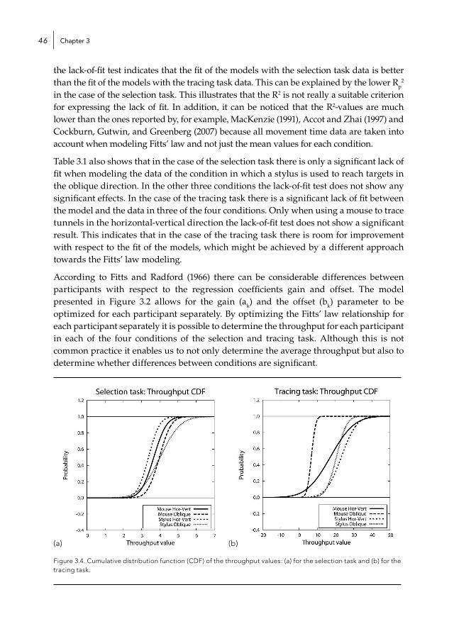
Chapter 346
the lack-of-fit test indicates that the fit of the models with the selection task data is better than the fit of the models with the tracing task data. This can be explained by the lower Rp
2
in the case of the selection task. This illustrates that the R2 is not really a suitable criterion for expressing the lack of fit. In addition, it can be noticed that the R2-values are much lower than the ones reported by, for example, MacKenzie (1991), Accot and Zhai (1997) and Cockburn, Gutwin, and Greenberg (2007) because all movement time data are taken into account when modeling Fitts’ law and not just the mean values for each condition.
Table 3.1 also shows that in the case of the selection task there is only a significant lack of fit when modeling the data of the condition in which a stylus is used to reach targets in the oblique direction. In the other three conditions the lack-of-fit test does not show any significant effects. In the case of the tracing task there is a significant lack of fit between the model and the data in three of the four conditions. Only when using a mouse to trace tunnels in the horizontal-vertical direction the lack-of-fit test does not show a significant result. This indicates that in the case of the tracing task there is room for improvement with respect to the fit of the models, which might be achieved by a different approach towards the Fitts’ law modeling.
According to Fitts and Radford (1966) there can be considerable differences between participants with respect to the regression coefficients gain and offset. The model presented in Figure 3.2 allows for the gain (ak) and the offset (bk) parameter to be optimized for each participant separately. By optimizing the Fitts’ law relationship for each participant separately it is possible to determine the throughput for each participant in each of the four conditions of the selection and tracing task. Although this is not common practice it enables us to not only determine the average throughput but also to determine whether differences between conditions are significant.
(a) (b)
Figure 3.4. Cumulative distribution function (CDF) of the throughput values: (a) for the selection task and (b) for the tracing task.
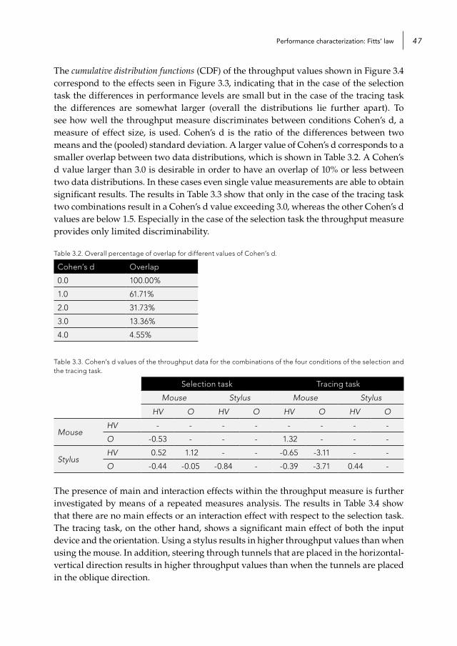
Performance characterization: Fitts’ law 47
The cumulative distribution functions (CDF) of the throughput values shown in Figure 3.4 correspond to the effects seen in Figure 3.3, indicating that in the case of the selection task the differences in performance levels are small but in the case of the tracing task the differences are somewhat larger (overall the distributions lie further apart). To see how well the throughput measure discriminates between conditions Cohen’s d, a measure of effect size, is used. Cohen’s d is the ratio of the differences between two means and the (pooled) standard deviation. A larger value of Cohen’s d corresponds to a smaller overlap between two data distributions, which is shown in Table 3.2. A Cohen’s d value larger than 3.0 is desirable in order to have an overlap of 10% or less between two data distributions. In these cases even single value measurements are able to obtain significant results. The results in Table 3.3 show that only in the case of the tracing task two combinations result in a Cohen’s d value exceeding 3.0, whereas the other Cohen’s d values are below 1.5. Especially in the case of the selection task the throughput measure provides only limited discriminability.
Table 3.2. Overall percentage of overlap for different values of Cohen’s d.
Cohen’s d Overlap
0.0 100.00%
1.0 61.71%
2.0 31.73%
3.0 13.36%
4.0 4.55%
Table 3.3. Cohen’s d values of the throughput data for the combinations of the four conditions of the selection and the tracing task.
Selection task Tracing task
Mouse Stylus Mouse Stylus
HV O HV O HV O HV O
MouseHV - - - - - - - -
O -0.53 - - - 1.32 - - -
StylusHV 0.52 1.12 - - -0.65 -3.11 - -
O -0.44 -0.05 -0.84 - -0.39 -3.71 0.44 -
The presence of main and interaction effects within the throughput measure is further investigated by means of a repeated measures analysis. The results in Table 3.4 show that there are no main effects or an interaction effect with respect to the selection task. The tracing task, on the other hand, shows a significant main effect of both the input device and the orientation. Using a stylus results in higher throughput values than when using the mouse. In addition, steering through tunnels that are placed in the horizontal-vertical direction results in higher throughput values than when the tunnels are placed in the oblique direction.
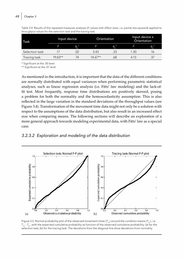
Chapter 348
Table 3.4. Results of the repeated measures analyses (F-values with effect sizes, i.e. partial eta-squared) applied to throughput values for the selection task and the tracing task.
TaskInput device Orientation Input device x
Orientation
F ηp2 F ηp
2 F ηp2
Selection task .17 .02 3.43 .33 1.30 .16
Tracing task 19.65** .74 14.67** .68 4.13 .37 * Significant at the .05 level ** Significant at the .01 level
As mentioned in the introduction, it is important that the data of the different conditions are normally distributed with equal variances when performing parametric statistical analyses, such as linear regression analysis (i.e. Fitts’ law modeling) and the lack-of-fit test. Most frequently, response time distributions are positively skewed, posing a problem for both the normality and the homoscedasticity assumption. This is also reflected in the large variation in the standard deviations of the throughput values (see Figure 3.4). Transformation of the movement time data might not only be a solution with respect to the assumptions of the data distribution, but also result in an increased effect size when comparing means. The following sections will describe an exploration of a more general approach towards modeling experimental data, with Fitts’ law as a special case.
3.2.3.2 Exploration and modeling of the data distribution
(a) (b)
Figure 3.5. Normal probability plot of the observed movement times (Tkij) around the condition means (Tki·), i.e. Tkij - Tki·, with the expected cumulative probability as function of the observed cumulative probability: (a) for the selection task; (b) for the tracing task. The deviations from the diagonal line show deviations from normality.

Performance characterization: Fitts’ law 49
In order to see if there are problems with the normality of the movement time data, P-P plots are created for the selection task data and the tracing task data (see Figure 3.5a and Figure 3.5b). The data of the different conditions should be normally distributed around the condition means, i.e. Tkij - Tki· ∼ N(0, σ). When the data is normally distributed, the data points should be placed on the diagonal line, which is also depitched in the graphs. Figure 3.5 clearly shows that the data deviates from this ideal line, especially in the case of the tracing task. This means that the data of the different conditions in both the selection task and the tracing task are not normally distributed around the conditional means. In addition, it can be observed that the tracing task data is somewhat more skewed than the selection task data, because the data deviates more from the ideal line.
(a) (b)
Figure 3.6. Normalized standard deviations (SD) of the observed movement times (Tkij) as function of the task characteristics (A=target distance, S=target size, L=tunnel length and W=tunnel width): (a) for the selection task; (b) for the tracing task. Participants (k) are treated as repetitions and in the graphs no distinction is made between the different orientations. The input devices, mouse or stylus, correspond to the drawn and dotted lines, respectively.
Figure 3.6a and Figure 3.6b show the variation in standard deviations for the selection task and tracing task, respectively. The variance of 36 conditions is compared: input device (2 levels) * orientation (2 levels) * task (9 levels). Especially the tracing task shows large differences in the standard deviation between the different task characteristics and between the input devices. The results of the Levene’s test for the equality of variances confirm that for both the selection task and the tracing task the variances of the different conditions are not homogenous, F(35,1100)=2.00, p<.01 and F(35,1116)=14.49, p<.001, respectively. With respect to the tracing task the Levene’s test also reveals that the variation in standard deviations is larger for the mouse, F(17,550)=13.05, p<.001 than for the stylus, F(17,550)=6.29, p<.001. This is not the case for the selection task where the variation in standard deviations is approximately the same for the mouse, F(17, 550)=2.08, p<.01 and the stylus, F(17,550)=2.02, p<.01.

Chapter 350
The exploration of the data distributions showed that a considerable amount of the data is not normally distributed and that there is no homogeneity of variance. Therefore, it needs to be determined whether a transformation should be applied to the data and, if so, what the optimal transformation would be. Field (2009) indicated that a logarithmic, a square root and a reciprocal transformation can be used to reduce a positive skew. In order to determine the appropriate transformation (i.e. value of p), the model in Figure 3.1 is applied to the selection task data and the tracing task data in which the data of all input devices and all participants are combined. Models with different values of the parameter p (see Equation (3.9)) are applied to the data: a linear model (p=1), a square root model (p=0.5), a logarithmic model (p=0) and a reciprocal model (p=-1) are compared to a model with the optimized value of p. The AIC values in Table 3.5 show that for the selection task data the model with the optimized value of parameter p (p=-.39) results in a significant better fit than the other models: in all comparisons the decrease in AIC is larger than 10. When these comparisons are applied to the tracing data the ∆AIC shows that also for the tracing task the optimized value of p (p=-.24) results in a significant better fit.
Table 3.5. AIC of the linear (p=1), square root (p=0.5), logarithmic (p=0) and reciprocal (p=-1) model in comparison to the optimized model.
TransformationSelection task Tracing task
AIC optimized (p=-.39) AIC optimized (p=-.24)
Linear (p=1) 386.52 944.08
Square root (p=0.5) 152.81 304.57
Logarithmic (p=0) 26.97 27.48
Reciprocal (p=-1) 63.69 224.68
(a) (b)
Figure 3.7. The log-likelihood profile (LLP) of parameter p: (a) for the selection task; (b) for the tracing task. Intersection with the horizontal line at X2
.05(1) = 3.84 indicates the 95% confidence interval for this parameter.

Performance characterization: Fitts’ law 51
Figure 3.7a and Figure 3.7b show the log-likelihood profile (LLP)2 of parameter p for the selection task and the tracing task. These figures show that there is a pronounced minimum for the LLP functions and that the value of p is significantly different from 1 and also from 0 (these values lie outside the indicated confidence interval). Although these results show that an optimized transformation (to accomplish a Gaussian distribution) is significantly better than a logarithmic transformation, these figures also show that a logarithmic transformation is better than a linear, a square root or a reciprocal transformation.
Figure 3.8 shows two P-P plots for the selection task. This figure shows the movement time data after a logarithmic transformation (see Figure 3.8a) and after an optimized transformation (see Figure 3.8b). When comparing both graphs to the graph in Figure 3.5a it can be seen that both transformations result in distributions that are closer to the normal distribution: the data points fall closer to the ideal diagonal line.
(a) (b)
Figure 3.8. Normal probability plot of the observed movement times (Tkij) around the condition means (Tki·), i.e. Tkij - Tki·, with the expected cumulative probability as function of the observed cumulative probability: (a) after logarithmic transformation (q=0); (b) after optimal transformation (q=-.39). The deviations from the diagonal line show deviations from normality.
Especially in the case of the tracing task the improvement of the shape of the distribution is clearly visible. Figure 3.9a shows the P-P plot of the movement time data after a logarithmic transformation and Figure 3.9b shows the P-P plot of the movement time data after an optimized transformation. Compared to the graph shown in Figure 3.5b both transformations result in distributions that are much closer to the normal distribution.
2 The log-likelihood profile (LLP) shows how much the LLC differs from its optimal value if one selected model parameter is varied around its optimal value, while the other model parameters are re-optimized for each new value of the selected parameter.

Chapter 352
(a) (b)
Figure 3.9. Normal probability plot of the observed movement times (Tkij) around the condition means (Tki·), i.e. Tkij - Tki·, with the expected cumulative probability as function of the observed cumulative probability: (a) after logarithmic transformation (q=0); (b) after optimal transformation (q=-.24). The deviations from the diagonal line show deviations from normality.
The maximum-likelihood estimation (MLE) optimizes the fit between the Gaussian models of constant variance and the histograms of the transformed data and, therefore, a correlation between a better fit and an equality of variance can be expected. The results of the Levene’s test for the equality of variances indeed show that after applying an optimized transformation the difference in variance decreases for both the selection task F(35,1100)=1.33 p=.11 and the tracing task F(35,1116)=2.47, p<.001. In the case of the selection task, the Levene’s test is not significant (p>.05), which means that the transformation results in data distributions with equal variances. In the case of the tracing task there are still some significant differences in the variances of the different conditions, but the reduction in the test statistics from F-value=14.49 to F-value=2.47 indicates a substantial improvement.
Table 3.6 shows the results of Levene’s tests after a linear, a square root, a logarithmic, a reciprocal or an optimized transformation is applied to the movement times of the selection task and the tracing task, respectively. In the case of the selection task the results show that the logarithmic transformation results in higher equality of variance than the optimized transformation (i.e. lowest F-value). In the case of the tracing task the optimized transformation results in the highest equality of variance (i.e. lowest F-value). The effect of the optimized transformation differs only minimally from that of the logarithmic transformation. In view of the small differences, and because it is a common practice to apply a logarithmic transformation to positively skewed time distributions, it is decided to use a logarithmic transformation rather than an optimized transformation for our movement times in our subsequent analyses.
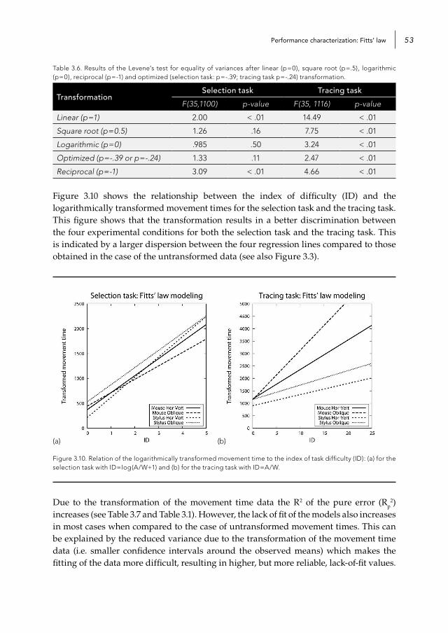
Performance characterization: Fitts’ law 53
Table 3.6. Results of the Levene’s test for equality of variances after linear (p=0), square root (p=.5), logarithmic (p=0), reciprocal (p=-1) and optimized (selection task: p=-.39; tracing task p=-.24) transformation.
TransformationSelection task Tracing task
F(35,1100) p-value F(35, 1116) p-value
Linear (p=1) 2.00 < .01 14.49 < .01
Square root (p=0.5) 1.26 .16 7.75 < .01
Logarithmic (p=0) .985 .50 3.24 < .01
Optimized (p=-.39 or p=-.24) 1.33 .11 2.47 < .01
Reciprocal (p=-1) 3.09 < .01 4.66 < .01
Figure 3.10 shows the relationship between the index of difficulty (ID) and the logarithmically transformed movement times for the selection task and the tracing task. This figure shows that the transformation results in a better discrimination between the four experimental conditions for both the selection task and the tracing task. This is indicated by a larger dispersion between the four regression lines compared to those obtained in the case of the untransformed data (see also Figure 3.3).
(a) (b)
Figure 3.10. Relation of the logarithmically transformed movement time to the index of task difficulty (ID): (a) for the selection task with ID=Iog(A/W+1) and (b) for the tracing task with ID=A/W.
Due to the transformation of the movement time data the R2 of the pure error (Rp2)
increases (see Table 3.7 and Table 3.1). However, the lack of fit of the models also increases in most cases when compared to the case of untransformed movement times. This can be explained by the reduced variance due to the transformation of the movement time data (i.e. smaller confidence intervals around the observed means) which makes the fitting of the data more difficult, resulting in higher, but more reliable, lack-of-fit values.

Chapter 354
Table 3.7. R2-values indicating the fit of the Fitts’ law model with the logarithmically transformed movement times for the selection task and the tracing task.
Device Orientation
Selection task Tracing task
R2 Rp2
Lack of FitR2 Rp
2Lack of fit
F p F p
MouseHor-Vert .40 .42 .98 .45 .52 .56 4.14 <.01
Oblique .40 .41 .63 .73 .71 .77 9.96 <.01
StylusHor-Vert .42 .46 3.08 <.01 .54 .70 21.50 <.01
Oblique .43 .45 1.73 .10 .52 .64 13.20 <.01
The cumulative distributions of the throughput values (see Figure 3.11) are further indications of the fact that the transformation of the movement times improves the discrimination between the experimental conditions. The Cohen’s d values in Table 3.8 confirm these findings: in most cases the Cohen’s d value is higher when the throughput values are based on the logarithmically transformed movement times than in the case of the measured movement times (see also Table 3.3). Another benefit of the transformation of the movement times is the increased equality of variance of the throughput values (see Figure 3.11), especially in the case of the tracing task (see also Figure 3.4).
(a) (b)Figure 3.11. Cumulative distribution function (CDF) of the throughput values based on the logarithmically transformed movement times: (a) for the selection task and (b) for the tracing task.
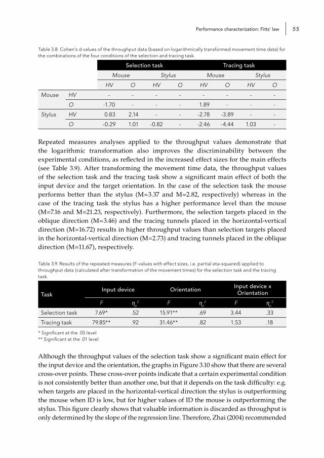
Performance characterization: Fitts’ law 55
Table 3.8. Cohen’s d values of the throughput data (based on logarithmically transformed movement time data) for the combinations of the four conditions of the selection and tracing task.
Selection task Tracing task
Mouse Stylus Mouse Stylus
HV O HV O HV O HV O
Mouse HV - - - - - - - -
O -1.70 - - - 1.89 - - -
Stylus HV 0.83 2.14 - - -2.78 -3.89 - -
O -0.29 1.01 -0.82 - -2.46 -4.44 1.03 -
Repeated measures analyses applied to the throughput values demonstrate that the logarithmic transformation also improves the discriminability between the experimental conditions, as reflected in the increased effect sizes for the main effects (see Table 3.9). After transforming the movement time data, the throughput values of the selection task and the tracing task show a significant main effect of both the input device and the target orientation. In the case of the selection task the mouse performs better than the stylus (M=3.37 and M=2.82, respectively) whereas in the case of the tracing task the stylus has a higher performance level than the mouse (M=7.16 and M=21.23, respectively). Furthermore, the selection targets placed in the oblique direction (M=3.46) and the tracing tunnels placed in the horizontal-vertical direction (M=16.72) results in higher throughput values than selection targets placed in the horizontal-vertical direction (M=2.73) and tracing tunnels placed in the oblique direction (M=11.67), respectively.
Table 3.9. Results of the repeated measures (F-values with effect sizes, i.e. partial eta-squared) applied to throughput data (calculated after transformation of the movement times) for the selection task and the tracing task.
TaskInput device Orientation Input device x
Orientation
F ηp2 F ηp
2 F ηp2
Selection task 7.69* .52 15.91** .69 3.44 .33
Tracing task 79.85** .92 31.46** .82 1.53 .18 * Significant at the .05 level** Significant at the .01 level
Although the throughput values of the selection task show a significant main effect for the input device and the orientation, the graphs in Figure 3.10 show that there are several cross-over points. These cross-over points indicate that a certain experimental condition is not consistently better than another one, but that it depends on the task difficulty: e.g. when targets are placed in the horizontal-vertical direction the stylus is outperforming the mouse when ID is low, but for higher values of ID the mouse is outperforming the stylus. This figure clearly shows that valuable information is discarded as throughput is only determined by the slope of the regression line. Therefore, Zhai (2004) recommended
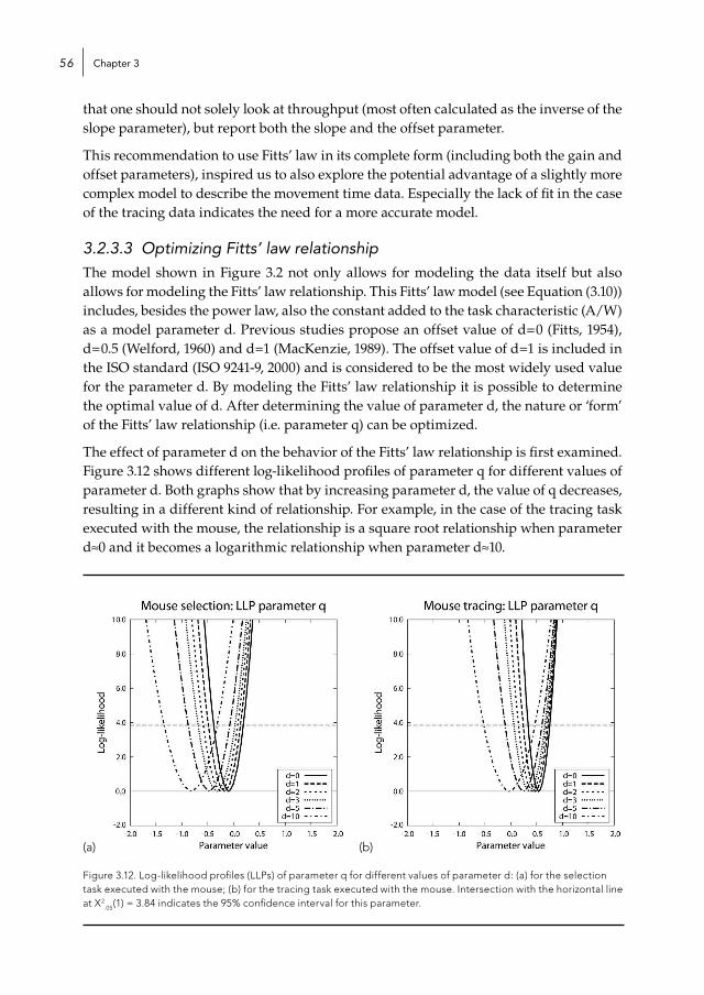
Chapter 356
that one should not solely look at throughput (most often calculated as the inverse of the slope parameter), but report both the slope and the offset parameter.
This recommendation to use Fitts’ law in its complete form (including both the gain and offset parameters), inspired us to also explore the potential advantage of a slightly more complex model to describe the movement time data. Especially the lack of fit in the case of the tracing data indicates the need for a more accurate model.
3.2.3.3 Optimizing Fitts’ law relationshipThe model shown in Figure 3.2 not only allows for modeling the data itself but also allows for modeling the Fitts’ law relationship. This Fitts’ law model (see Equation (3.10)) includes, besides the power law, also the constant added to the task characteristic (A/W) as a model parameter d. Previous studies propose an offset value of d=0 (Fitts, 1954), d=0.5 (Welford, 1960) and d=1 (MacKenzie, 1989). The offset value of d=1 is included in the ISO standard (ISO 9241-9, 2000) and is considered to be the most widely used value for the parameter d. By modeling the Fitts’ law relationship it is possible to determine the optimal value of d. After determining the value of parameter d, the nature or ‘form’ of the Fitts’ law relationship (i.e. parameter q) can be optimized.
The effect of parameter d on the behavior of the Fitts’ law relationship is first examined. Figure 3.12 shows different log-likelihood profiles of parameter q for different values of parameter d. Both graphs show that by increasing parameter d, the value of q decreases, resulting in a different kind of relationship. For example, in the case of the tracing task executed with the mouse, the relationship is a square root relationship when parameter d 0 and it becomes a logarithmic relationship when parameter d 10.
(a) (b)
Figure 3.12. Log-likelihood profiles (LLPs) of parameter q for different values of parameter d: (a) for the selection task executed with the mouse; (b) for the tracing task executed with the mouse. Intersection with the horizontal line at X2
.05(1) = 3.84 indicates the 95% confidence interval for this parameter.
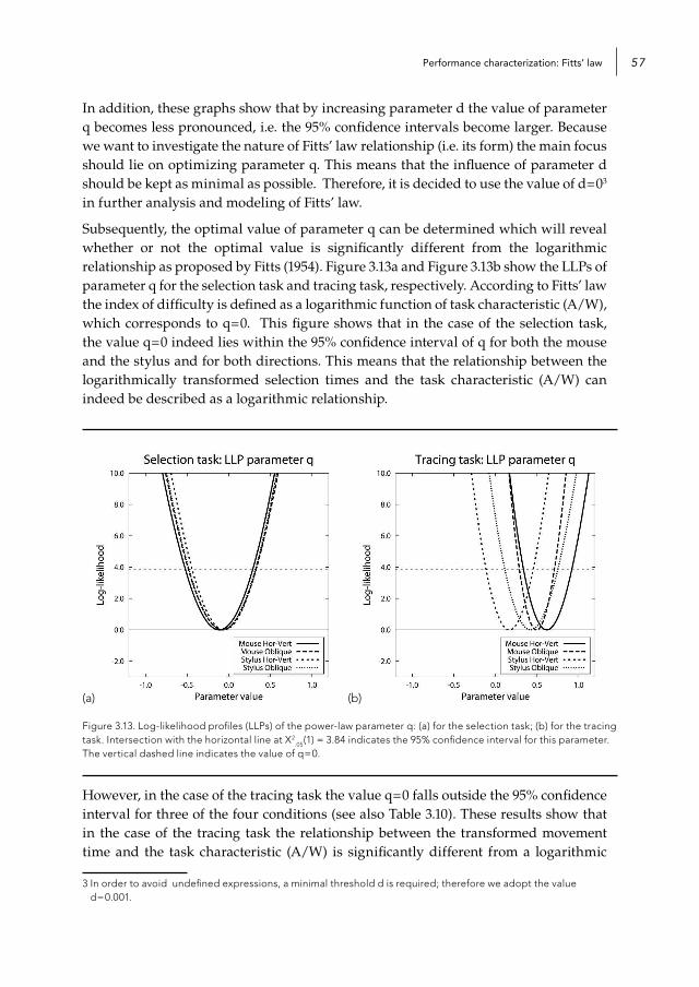
Performance characterization: Fitts’ law 57
In addition, these graphs show that by increasing parameter d the value of parameter q becomes less pronounced, i.e. the 95% confidence intervals become larger. Because we want to investigate the nature of Fitts’ law relationship (i.e. its form) the main focus should lie on optimizing parameter q. This means that the influence of parameter d should be kept as minimal as possible. Therefore, it is decided to use the value of d=03
in further analysis and modeling of Fitts’ law.
Subsequently, the optimal value of parameter q can be determined which will reveal whether or not the optimal value is significantly different from the logarithmic relationship as proposed by Fitts (1954). Figure 3.13a and Figure 3.13b show the LLPs of parameter q for the selection task and tracing task, respectively. According to Fitts’ law the index of difficulty is defined as a logarithmic function of task characteristic (A/W), which corresponds to q=0. This figure shows that in the case of the selection task, the value q=0 indeed lies within the 95% confidence interval of q for both the mouse and the stylus and for both directions. This means that the relationship between the logarithmically transformed selection times and the task characteristic (A/W) can indeed be described as a logarithmic relationship.
(a) (b)
Figure 3.13. Log-likelihood profiles (LLPs) of the power-law parameter q: (a) for the selection task; (b) for the tracing task. Intersection with the horizontal line at X2
.05(1) = 3.84 indicates the 95% confidence interval for this parameter. The vertical dashed line indicates the value of q=0.
However, in the case of the tracing task the value q=0 falls outside the 95% confidence interval for three of the four conditions (see also Table 3.10). These results show that in the case of the tracing task the relationship between the transformed movement time and the task characteristic (A/W) is significantly different from a logarithmic
3 In order to avoid undefined expressions, a minimal threshold d is required; therefore we adopt the value d=0.001.
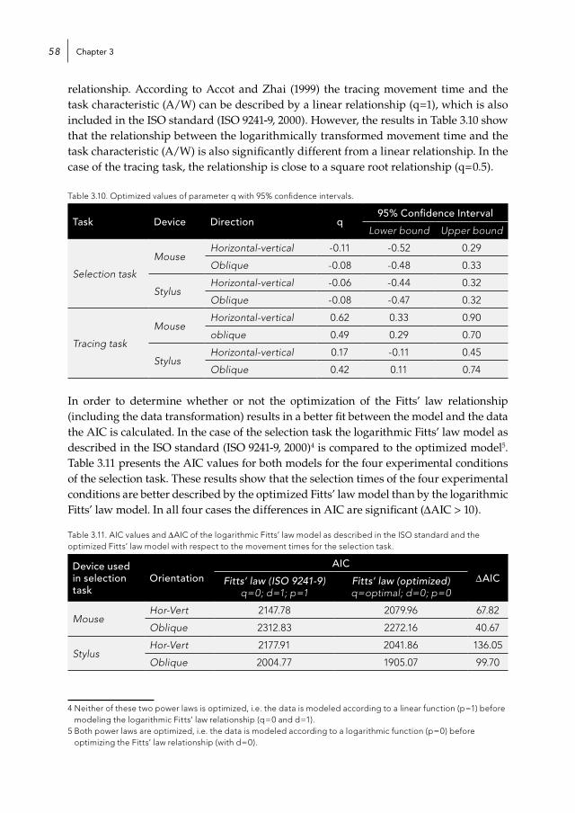
Chapter 358
relationship. According to Accot and Zhai (1999) the tracing movement time and the task characteristic (A/W) can be described by a linear relationship (q=1), which is also included in the ISO standard (ISO 9241-9, 2000). However, the results in Table 3.10 show that the relationship between the logarithmically transformed movement time and the task characteristic (A/W) is also significantly different from a linear relationship. In the case of the tracing task, the relationship is close to a square root relationship (q=0.5).
Table 3.10. Optimized values of parameter q with 95% confidence intervals.
Task Device Direction q95% Confidence Interval
Lower bound Upper bound
Selection task
MouseHorizontal-vertical -0.11 -0.52 0.29
Oblique -0.08 -0.48 0.33
StylusHorizontal-vertical -0.06 -0.44 0.32
Oblique -0.08 -0.47 0.32
Tracing task
MouseHorizontal-vertical 0.62 0.33 0.90
oblique 0.49 0.29 0.70
StylusHorizontal-vertical 0.17 -0.11 0.45
Oblique 0.42 0.11 0.74
In order to determine whether or not the optimization of the Fitts’ law relationship (including the data transformation) results in a better fit between the model and the data the AIC is calculated. In the case of the selection task the logarithmic Fitts’ law model as described in the ISO standard (ISO 9241-9, 2000)4 is compared to the optimized model5. Table 3.11 presents the AIC values for both models for the four experimental conditions of the selection task. These results show that the selection times of the four experimental conditions are better described by the optimized Fitts’ law model than by the logarithmic Fitts’ law model. In all four cases the differences in AIC are significant (∆AIC > 10).
Table 3.11. AIC values and ∆AIC of the logarithmic Fitts’ law model as described in the ISO standard and the optimized Fitts’ law model with respect to the movement times for the selection task.
Device used in selection task
OrientationAIC
∆AICFitts’ law (ISO 9241-9) q=0; d=1; p=1
Fitts’ law (optimized) q=optimal; d=0; p=0
MouseHor-Vert 2147.78 2079.96 67.82
Oblique 2312.83 2272.16 40.67
StylusHor-Vert 2177.91 2041.86 136.05
Oblique 2004.77 1905.07 99.70
4 Neither of these two power laws is optimized, i.e. the data is modeled according to a linear function (p=1) before modeling the logarithmic Fitts’ law relationship (q=0 and d=1).
5 Both power laws are optimized, i.e. the data is modeled according to a logarithmic function (p=0) before optimizing the Fitts’ law relationship (with d=0).
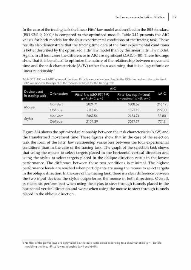
Performance characterization: Fitts’ law 59
In the case of the tracing task the linear Fitts’ law model as described in the ISO standard (ISO 9241-9, 2000)6 is compared to the optimized model5. Table 3.12 presents the AIC values for both models for the four experimental conditions of the tracing task. These results also demonstrate that the tracing time data of the four experimental conditions is better described by the optimized Fitts’ law model than by the linear Fitts’ law model. Again, in all four cases the differences in AIC are significant (∆AIC > 10). These findings show that it is beneficial to optimize the nature of the relationship between movement time and the task characteristic (A/W) rather than assuming that it is a logarithmic or linear relationship.
Table 3.12. AIC and ∆AIC values of the linear Fitts’ law model as described in the ISO standard and the optimized Fitts’ law model with respect to the movement times for the tracing task.
Device used in tracing task Orientation
AIC ∆AICFitts’ law (ISO 9241-9)
q=1; d=0; p=1Fitts’ law (optimized) q=optimal; d=0; p=0
MouseHor-Vert 2024.71 1808.52 216.19
Oblique 2112.45 1893.15 219.30
StylusHor-Vert 2467.54 2434.74 32.80
Oblique 2104.39 2027.27 77.12
Figure 3.14 shows the optimized relationship between the task characteristic (A/W) and the transformed movement time. These figures show that in the case of the selection task the form of the Fitts’ law relationship varies less between the four experimental conditions than in the case of the tracing task. The graph of the selection task shows that using the mouse to select targets placed in the horizontal-vertical direction and using the stylus to select targets placed in the oblique direction result in the lowest performance. The difference between these two conditions is minimal. The highest performance levels are reached when participants are using the mouse to select targets in the oblique direction. In the case of the tracing task, there is a clear difference between the two input devices: the stylus outperforms the mouse in both directions. Overall, participants perform best when using the stylus to steer through tunnels placed in the horizontal-vertical direction and worst when using the mouse to steer through tunnels placed in the oblique direction.
6 Neither of the power laws are optimized, i.e. the data is modeled according to a linear function (p=1) before modeling the linear Fitts’ law relationship (q=1 and d=0).

Chapter 360
(a) (b)
Figure 3.14. Optimized relation of the logarithmically transformed movement time to the task characteristic (A/W): (a) for the selection task and (b) for the tracing task.
The optimization of the Fitts’ law relationship do not result in higher Rp2 values (see
Table 3.13 and Table 3.7). However, the results of the lack-of-fit test show that the model’s fit is somewhat better in the case of the optimized Fitts’ law relationship (see Table 3.13) than in the case of the logarithmic Fitts’ law relationship (see Table 3.7). The differences are somewhat larger for the tracing task than for the selection task. Nevertheless, in the case of the tracing task the lack-of-fit values are still significant, indicating that there is still room for improvement.
Table 3.13. R2-values indicating the fit of the optimized Fitts’ law model for the selection task and the tracing task.
Device Orientation
Selection task Tracing task
R2 Rp2
Lack of FitR2 Rp
2Lack of fit
F p F p
MouseHor-Vert .40 .42 .87 .53 .53 .56 3.47 <.01
Oblique .40 .41 .56 .79 .73 .77 6.75 <.01
StylusHor-Vert .42 .46 3.02 <.01 .58 .70 16.00 <.01
Oblique .43 .45 1.64 .13 .54 .64 11.22 <.01
Calculating throughput when the relationship between the task characteristic (A/W) and the transformed movement time is optimized, does not only discard the variation in the offset (parameter a) but also the variation in the form of the relationship (parameter q). Throughput is hence not suitable to characterize performance as a single measure. In order to compare experimental conditions with each other we propose an alternative performance rate (PR) measure that takes into account the offset, gain and form of the
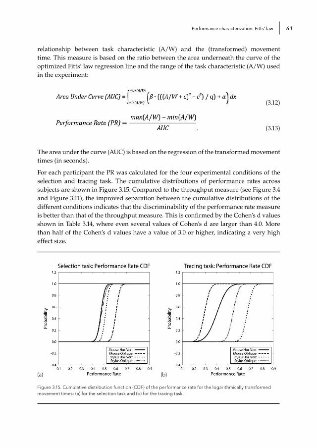
Performance characterization: Fitts’ law 61
relationship between task characteristic (A/W) and the (transformed) movement time. This measure is based on the ratio between the area underneath the curve of the optimized Fitts’ law regression line and the range of the task characteristic (A/W) used in the experiment:
(3.12)
. (3.13)
The area under the curve (AUC) is based on the regression of the transformed movement times (in seconds).
For each participant the PR was calculated for the four experimental conditions of the selection and tracing task. The cumulative distributions of performance rates across subjects are shown in Figure 3.15. Compared to the throughput measure (see Figure 3.4 and Figure 3.11), the improved separation between the cumulative distributions of the different conditions indicates that the discriminability of the performance rate measure is better than that of the throughput measure. This is confirmed by the Cohen’s d values shown in Table 3.14, where even several values of Cohen’s d are larger than 4.0. More than half of the Cohen’s d values have a value of 3.0 or higher, indicating a very high effect size.
(a) (b)
Figure 3.15. Cumulative distribution function (CDF) of the performance rate for the logarithmically transformed movement times: (a) for the selection task and (b) for the tracing task.
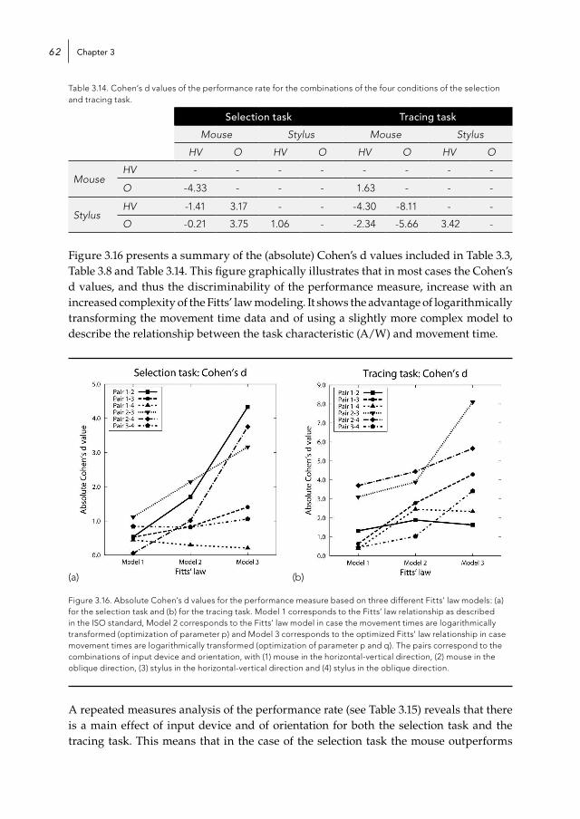
Chapter 362
Table 3.14. Cohen’s d values of the performance rate for the combinations of the four conditions of the selection and tracing task.
Selection task Tracing task
Mouse Stylus Mouse Stylus
HV O HV O HV O HV O
MouseHV - - - - - - - -
O -4.33 - - - 1.63 - - -
StylusHV -1.41 3.17 - - -4.30 -8.11 - -
O -0.21 3.75 1.06 - -2.34 -5.66 3.42 -
Figure 3.16 presents a summary of the (absolute) Cohen’s d values included in Table 3.3, Table 3.8 and Table 3.14. This figure graphically illustrates that in most cases the Cohen’s d values, and thus the discriminability of the performance measure, increase with an increased complexity of the Fitts’ law modeling. It shows the advantage of logarithmically transforming the movement time data and of using a slightly more complex model to describe the relationship between the task characteristic (A/W) and movement time.
(a) (b)
Figure 3.16. Absolute Cohen’s d values for the performance measure based on three different Fitts’ law models: (a) for the selection task and (b) for the tracing task. Model 1 corresponds to the Fitts’ law relationship as described in the ISO standard, Model 2 corresponds to the Fitts’ law model in case the movement times are logarithmically transformed (optimization of parameter p) and Model 3 corresponds to the optimized Fitts’ law relationship in case movement times are logarithmically transformed (optimization of parameter p and q). The pairs correspond to the combinations of input device and orientation, with (1) mouse in the horizontal-vertical direction, (2) mouse in the oblique direction, (3) stylus in the horizontal-vertical direction and (4) stylus in the oblique direction.
A repeated measures analysis of the performance rate (see Table 3.15) reveals that there is a main effect of input device and of orientation for both the selection task and the tracing task. This means that in the case of the selection task the mouse outperforms
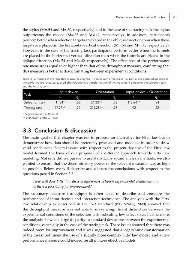
Performance characterization: Fitts’ law 63
the stylus (M=.54 and M=.50, respectively) and in the case of the tracing task the stylus outperforms the mouse (M=.35 and M=.42, respectively). In addition, participants perform better when selection targets are placed in the oblique direction than when these targets are placed in the horizontal-vertical direction (M=.54 and M=.50, respectively). However, in the case of the tracing task participants perform better when the tunnels are placed in the horizontal-vertical direction than when the tunnels are placed in the oblique direction (M=.54 and M=.42, respectively). The effect size of the performance rate measure is equal to or higher than that of the throughput measure, confirming that this measure is better at discriminating between experimental conditions.
Table 3.15. Results of the repeated measures analysis (F-values with effect sizes, i.e. partial eta-squared) applied to the performance rates (calculated after logarithmic transformation of the movement times) for the selection task and the tracing task.
TaskInput device Orientation Input device x Orientation
F ηp2 F ηp
2 F ηp2
Selection task 11.24* .62 24.33** .78 112.64** .94
Tracing task 77.97** .92 371.28** .98 .92 .12
* Significant at the .05 level** Significant at the .01 level
3.3 Conclusion & discussionThe main goal of this chapter was not to propose an alternative for Fitts’ law but to demonstrate how data should be preferably processed and modeled in order to draw valid conclusions. Several issues with respect to the present-day use of the Fitts’ law model formed the basis of our proposal of a different approach towards Fitts’ law modeling. Not only did we pursue to use statistically sound analysis methods, we also wanted to ensure that the discriminatory power of the relevant measures was as high as possible. Below we will describe and discuss the conclusions with respect to the questions posed in Section 3.2.1.
How well does Fitts’ law discern differences between experimental conditions and is there a possibility for improvement?
The summary measure throughput is often used to describe and compare the performance of input devices and interaction techniques. The analysis with the Fitts’ law relationship as described in the ISO standard (ISO 9241-9, 2000) showed that the throughput measure was not able to make a significant distinction between the experimental conditions of the selection task indicating low effect sizes. Furthermore, the analysis showed a large disparity in standard deviations between the experimental conditions, especially in the case of the tracing task. These issues showed that there was indeed room for improvement and it was suggested that a logarithmic transformation of the measured times, the use of a slightly more complex Fitts’ law model, and a new performance measure could indeed result in more effective models.

Chapter 364
Are there problems with the normality and homogeneity of the movement time data and is transformation of the data required?
The data showed that there were indeed problems with the normality and homogeneity of the movement time data. Especially in the case of the tracing task the data was highly skewed and there was a large variation in the variances across conditions. After applying transformations to the data there was a large improvement with respect to the normality and the homogeneity of the data. In addition, the discriminatory power of the summary measure throughput also increased, revealing some additional significant effects between the experimental conditions. Therefore, it could be concluded that transformation of movement time was required before applying parametrical statistical analyses that assume that the data of the various conditions is normally distributed with equal variances. This transformation will place the data on a scale that is linearly interpretable, which makes effect size comparisons possible.
What kind of model (e.g. linear, logarithmic or power-law) describes the relationship between movement time and the task characteristic best?
The optimization of the Fitts’ law model showed that in the case of the selection task the relationship between the task characteristic and the logarithmically transformed movement time was indeed well approximated by a logarithmic relationship. However, in the case of the tracing task, there was a considerable discrepancy between the values for the optimal transformation (parameter q) from 0 (a logarithmic transformation) and 1 (no transformation). This led us to conclude that a power-law function instead of the predetermined logarithmic or linear function is better to describe the relationship between the task characteristic (A/W) and movement time.
Although the optimized model was slightly more complex than the original Fitts’ law model, the more accurate description of the relationship, the increased fit of the data and the better discrimination between experimental conditions outweighed the disadvantage of including an additional parameter in the model. A solution for the increased complexity was also offered in the form of the performance rate measure that did not only take into account the offset but also the gain and the form of the relationship between the task characteristic (A/W) and the (logarithmically transformed) movement times.
What are the benefits of optimizing the Fitts’ law relationship?
We demonstrated that the fit of the Fitts’ law model could be improved by applying a transformation to the movement time data and by optimizing the Fitts’ law relationship. This resulted not only in data distributions that were more normally distributed with a higher equality of variances but also in larger effect sizes, especially for the newly proposed measure of performance rate. The benefits of these outcomes were that the conclusions drawn from the results were not only more statistically sound, but also more accurate (due to the better fit) and more convincing (due to the larger effect sizes). In other words, the optimization of the Fitts’ law relationship allowed for a higher contrast between variables such as input devices and interaction techniques.

Performance characterization: Fitts’ law 65
- - -
Throughput and performance rate are summary statistics that can point out differences between experimental conditions. Although the proposed approach towards Fitts’ law modeling of movement time data results in more robust and methodologically sound conclusions, it does not assist in understanding the underlying reasons for the performance differences. In other words, it does not describe in what way the performance of certain input devices or interaction techniques are different. More information can be gathered with respect to the movement quality besides movement time, which is simply based on the registration of the begin- and endpoint of a movement. As a matter of fact, there are already a vast amount of measures to characterize the movement path or the velocity profile. However, when aiming at providing a clear view of the movement quality, it is preferable to have only a limited number of measures that can capture different aspects of the movement behavior. In the next chapter we will investigate to what extent measures characterizing different properties of the movement (i.e. movement path and velocity profile) are complementary to each other and how measures can be selected to provide an appropriate description of movement quality.

Chapter 366

Chapter 4
Movement characterization

Chapter 468
4.1 Measures characterizing movement qualityTo determine which input device or interaction technique performs best, numerous measures have been proposed that can be derived from the executed movement. The complexity of these measures and the effort required to derive the measures from the executed movement varies considerably. Some of the proposed measures can be easily derived from the registration of the begin- and endpoint of the movement, others are more complex and require frequent path sampling and extensive computation. By providing a summary description of the movement, these measures can assist in understanding why a particular input device or interaction technique is faster in use than another one.
With numerous possible measures to apply, the question arises how we can select a handful of measures that are able to provide an adequate description of the movement quality. Our aim is not to end up with a fixed selection of measures to be used in the evaluation of input devices and interaction techniques, but to describe a process of how to select a few measures from a large set of alternatives. We want to support the selection process by providing insights into the possible added value of more complex measures and propose a selection procedure that is aimed at addressing a specific question. The measures1 we will take into account in this exploration can be divided in three clusters, based on the derivation method: a) begin- and endpoint measures, b) position-based measures and c) velocity-based measures1.
4.1.1 Begin- and endpoint measuresThe simplest way of recording performance on selection and pointing tasks is to register the begin- and endpoints of a movement, e.g. by logging the discrete button clicks when people are using a computer mouse or stylus. This method of logging data is relatively simple and it does not result in large amounts of data that require extensive data analysis. The measures that are most frequently derived from the begin- and endpoint registration are movement time (also referred to as movement duration, task completion time, positioning time and overall time), the number of errors and/or the error rate (i.e. percentage of trials containing errors).
Zhai, Buxton and Milgram (1994) used the measure ‘error magnitude’ to communicate the size of the errors made during task performance. The error magnitude is defined as the Euclidean distance from the position where the error occurred to the target location. In the case of a selection task this will correspond to the distance between the position of the cursor at the time of the button click (outside the target area) and the target boundary. In the case of a tracing task this will correspond to the distance between the position of the cursor when leaving the tunnel and the boundary of the target area. A disadvantage of this measure is that it does not contain any values when no errors occur.
1 We will only consider measures that can be derived from a single movement.

Movement characterization 69
4.1.2 Position-based measuresMacKenzie, Kauppinen & Silfverberg (2001) acknowledged that speed-accuracy measures like movement time and error rates are “gross measures” and that they lack “any information on the movement during a trial”. Therefore, they suggested that more thorough analyses of the movement path would be necessary to establish why some input devices or interaction techniques result in higher performance. To look at the movement path in more detail it is necessary to frequently log the pointer position, which requires a more complex data processing method.
4.1.2.1 Accuracy measuresMacKenzie et al. (2001) proposed four discrete accuracy measures and three continuous accuracy measures, which intend to quantify smoothness (or lack of it) in pointer movement. According to them these measures can capture movement variation that cannot be captured by “accuracy measures based only on end-point variation”.
Table 4.1. Description of the discrete accuracy measures proposed by MacKenzie et al. (2001) assessing the pointer deviation from the ‘perfect target selection task’.
Measure Description Illustration
Target re-entryOccurs when the pointer enters, leaves and enters the target area again.
Task axis crossing
Occurs when the pointer crosses the task axis (line connecting the starting point to the target center).
Movement direction change
Occurs when direction changes in pointer’s path are parallel to the task axis (local extreme values orthogonal to the task axis).
Orthogonal direction change
Occurs when direction changes in pointer’s path are orthogonal to the task axis (local extreme values parallel to the task axis).
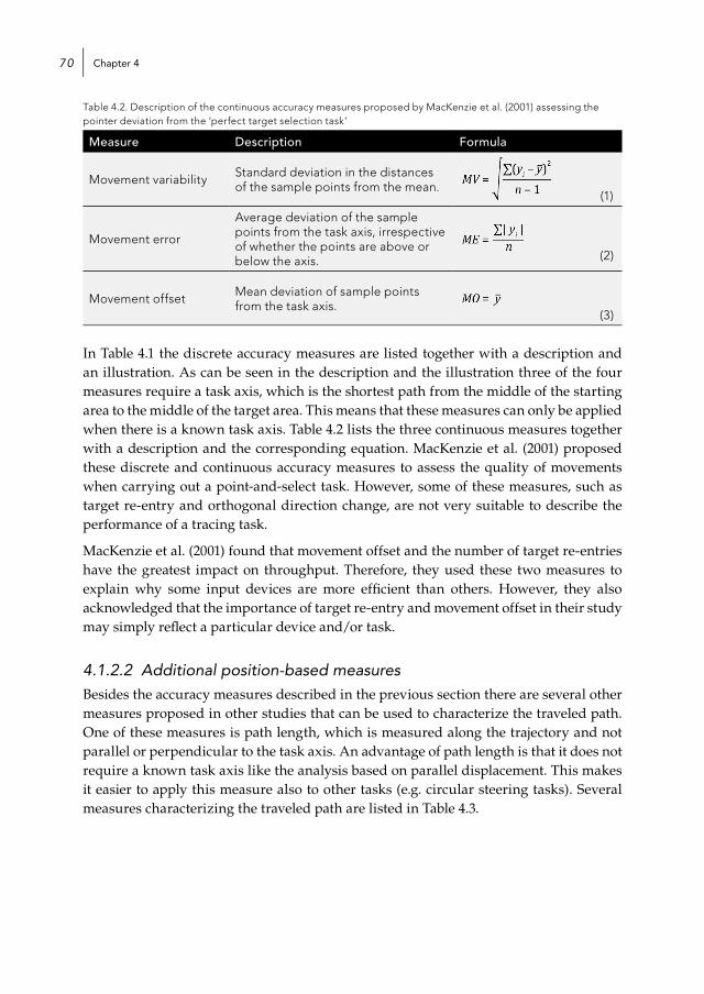
Chapter 470
Table 4.2. Description of the continuous accuracy measures proposed by MacKenzie et al. (2001) assessing the pointer deviation from the ‘perfect target selection task’
Measure Description Formula
Movement variability Standard deviation in the distances of the sample points from the mean.
(1)
Movement error
Average deviation of the sample points from the task axis, irrespective of whether the points are above or below the axis. (2)
Movement offset Mean deviation of sample points from the task axis.
(3)
In Table 4.1 the discrete accuracy measures are listed together with a description and an illustration. As can be seen in the description and the illustration three of the four measures require a task axis, which is the shortest path from the middle of the starting area to the middle of the target area. This means that these measures can only be applied when there is a known task axis. Table 4.2 lists the three continuous measures together with a description and the corresponding equation. MacKenzie et al. (2001) proposed these discrete and continuous accuracy measures to assess the quality of movements when carrying out a point-and-select task. However, some of these measures, such as target re-entry and orthogonal direction change, are not very suitable to describe the performance of a tracing task.
MacKenzie et al. (2001) found that movement offset and the number of target re-entries have the greatest impact on throughput. Therefore, they used these two measures to explain why some input devices are more effi cient than others. However, they also acknowledged that the importance of target re-entry and movement offset in their study may simply refl ect a particular device and/or task.
4.1.2.2 Additional position-based measuresBesides the accuracy measures described in the previous section there are several other measures proposed in other studies that can be used to characterize the traveled path. One of these measures is path length, which is measured along the trajectory and not parallel or perpendicular to the task axis. An advantage of path length is that it does not require a known task axis like the analysis based on parallel displacement. This makes it easier to apply this measure also to other tasks (e.g. circular steering tasks). Several measures characterizing the traveled path are listed in Table 4.3.

Movement characterization 71
Table 4.3. Description of the position-based measures.
Measure Description Reference
Path length Length of traveled path.(Adam et al., 1995; Teulings, Contreras-Vidal, Stelmach, & Adler, 1997)
Path length efficiency
Ratio between the traveled path and the shortest path. (Keates & Trewin, 2005)
High curvature analysis
Number of times the angle between 3 successive sample points is less than 80 deg.
(Goldvasser, McGibbon, & Krebs, 2001)
Final positioning time
Interval from (the last) target entry until the end of the trial.
(Akamatsu, MacKenzie, & Hasbroucq, 1995; Behbehani, Kondraske, & Richmond, 1988)
In addition, some characteristics that can be derived from the path are related to whether or not the pointer traverses beyond the target area, i.e. overshoots the target area. Although these measures can be used to characterize the path of a selection movement, it is expected that they are not really suitable to characterize the path of a tracing movement. During the tracing task the trial is restarted once the pointer traverses beyond the boundaries of the target (or stop) area. Since the participants will be moving more cautiously to stay within the tunnel boundaries, overshoots will hardly occur. The overshoot measures are presented in Table 4.4.
Table 4.4. Description of the position-based measures, regarding target overshoots.
Measure Description Reference
Overshoot occurrence
Frequency of trials in which the pointer traverses beyond the target area (in the direction of the task axis).
(Buck, 1980)
Overshoot timeIn the case of an overshoot, the interval from the moment the cursor first traverses beyond the target area until the end of the trial.
(Behbehani et al., 1988; Buck, 1980)
Percentage of maximum overshoot
In the case of an overshoot, the largest percent deviation of the cursor from the target (based on parallel displacement) once it traverses beyond the target area.
(Behbehani et al., 1988)
Although position-based measures take into account information about the traveled path they do not take into account the detailed course of the movement as a function of time. Figure 4.1 shows not only the traveled path of a goal-directed movement, but also the corresponding path length (in percentage) over time. This graph shows that path length is not monotonically increasing which indicates that more information about the quality of movement can be derived from the executed movement. In the next section measures will be discussed that are based on the derivative of the traveled path, i.e. the movement velocity.
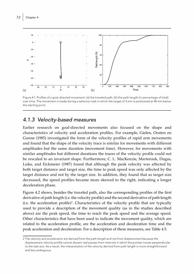
Chapter 472
(a) (b)
Figure 4.1. Profiles of a goal-directed movement: (a) the traveled path, (b) the path length (in percentage of total) over time. The movement is made during a selection task in which the target of 3 mm is positioned at 48 mm below the starting point.
4.1.3 Velocity-based measuresEarlier research on goal-directed movements also focused on the shape and characteristics of velocity and acceleration profiles. For example, Gielen, Oosten en Gunne (1985) investigated the form of the velocity profiles of rapid arm movements and found that the shape of the velocity trace is similar for movements with different amplitudes but the same duration (movement time). However, for movements with similar amplitudes but different durations the traces of the velocity profile could not be rescaled to an invariant shape. Furthermore, C. L. MacKenzie, Marteniuk, Dugas, Liske, and Eickmeier (1987) found that although the peak velocity was affected by both target distance and target size, the time to peak speed was only affected by the target distance and not by the target size. In addition, they found that as target size decreased, the speed profiles became more skewed to the right, indicating a longer deceleration phase.
Figure 4.2 shows, besides the traveled path, also the corresponding profiles of the first derivative of path length (i.e. the velocity profile) and the second derivative of path length (i.e. the acceleration profile)2. Characteristics of the velocity profile that are typically used to provide a description of the movement quality (as in the studies described above) are the peak speed, the time to reach the peak speed and the average speed. Other characteristics that have been used to indicate the movement quality, which are related to the acceleration profile, are the acceleration and deceleration time and the peak acceleration and deceleration. For a description of these measures, see Table 4.5.
2 The velocity and acceleration are derived from the path length and not from displacement because the displacement velocity profile cannot discern real pauses from intervals in which the pointer moves perpendicular to the task axis. As a result, the interpretation of the velocity derived from path length is more straightforward and less ambiguous.
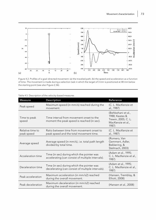
Movement characterization 73
(a) (b)
Figure 4.2. Profiles of a goal-directed movement: (a) the traveled path, (b) the speed and acceleration as a function of time. The movement is made during a selection task in which the target of 3 mm is positioned at 48 mm below the starting point (see also Figure 2.36).
Table 4.5. Description of the velocity-based measures.
Measure Description Reference
Peak speed Maximum speed (in mm/s) reached during the movement.
(C. L. MacKenzie et al., 1987)
Time to peak speed
Time interval from movement onset to the moment the peak speed is reached (in sec).
(Behbehani et al., 1988; Keates & Trewin, 2005; C. L. MacKenzie et al., 1987)
Relative time to peak speed
Ratio between time from movement onset to peak speed and the total movement time.
(C. L. MacKenzie et al., 1987)
Average speed Average speed (in mm/s), i.e. total path length divided by total time.
(Romero, Van Gemmert, Adler, Bekkering, & Stelmach, 2003)
Acceleration time Time (in sec) during which the pointer was accelerating (can consist of multiple intervals).
(Adam et al., 1995; C. L. MacKenzie et al., 1987)
Deceleration time Time (in sec) during which the pointer was decelerating (can consist of multiple intervals).
(Adam et al., 1995; C. L. MacKenzie et al., 1987)
Peak acceleration Maximum acceleration (in mm/s2) reached during the overall movement.
(Hansen, Tremblay, & Elliott, 2008)
Peak deceleration Maximum deceleration (in mm/s2) reached during the overall movement. (Hansen et al., 2008)

Chapter 474
When looking at the velocity profile in Figure 4.2 it can be noticed that this velocity profile does not have a fluent single bell-shaped form. These irregularities have traditionally been interpreted as corrective submovements performed when the primary initiated movement (or primary submovement) does not end at the target (Wisleder & Dounskaia, 2007). According to the Deterministic Iterative-Corrections Model (Crossman & Goodeve, 1983) each submovement travels a constant proportion of the remaining distance towards the center of the target (see Figure 4.3a). According to the Stochastic Optimized-Submovement Model (Meyer et al, 1988) the primary movement is programmed to reach the target center, but can miss the target due to noise in the motor system. In these cases a secondary submovement is immediately executed (see Figure 4.3b). Irrespective of the underlying movement model, these corrections can also be used to determine the movement quality.
(a) (b)
Figure 4.3. Movement models: (a) Deterministic Iterative-Corrections Model; (b) Stochastic Optimized-Submovement Model .
Meyer et al. (1988) proposed parsing criteria to indicate the end of the primary submovement. Dounskaia, Wisleder and Johnson (2005) used these parsing criteria to identify the type of submovements made during a movement. The measures with respect to the number and the type of submovements can be used to investigate the smoothness of the velocity profile. We adjusted the criteria to parse movements into submovements so they could be applied to speed profiles based on path length (Nieuwenhuizen, Aliakseyeu, & Martens, 2009a). We preferably use path length to determine the pointer’s speed because the displacement velocity profile cannot discern real pauses from intervals in which the pointer moves perpendicular to the task axis. In addition, the analysis based on path length does not require a known task axis like the analysis based on parallel displacement, which makes it easier to extend the method to other tasks (such as circular steering tasks). The following submovements can be identified3 (see Figure 4.4):
a. type-1 submovement starts when the speed becomes (almost) zero (less than 0.02 times the movement’s peak speed), which means that a submovement can only occur at the beginning of a movement interval;
b. type-2 submovement starts at a zero-crossing of acceleration from negative to positive (in combination with a positive jerk that exceeds 0.01 times the maximally observed jerk4) and hence corresponds to a local minimum in the velocity profile;
3 For the argumentation of the parsing criteria see Chapter 5.4 Jerk is the derivative of acceleration

Movement characterization 75
c. type-3 submovement starts at a zero-crossing of jerk from positive to negative (in combination with a negative value of its derivative that exceeds 0.01 times the maximally observed value).
Figure 4.4. Examples of a type-1, type-2 and type-3 submovement.
Type-1 submovements are considered to be coarse interruptions in the smoothness of the movement, whereas type-3 submovements are considered as subtle accuracy regulations. As mentioned before, the characterizations can be used to describe the quality of the velocity profile in terms of smoothness. Other measures indicating the smoothness of the velocity profile are related to the pauses occurring during the movement: more and longer pauses are associated with a lower movement quality. Table 4.6 shows the measures that are related to the smoothness of the velocity profile.
Table 4.6. Description of the velocity-based measures regarding the smoothness of the velocity profile.
Measure Description Reference
Number of submovements
Total number of submovements made during the overall movement.
(Walker, Meyer, & Smelcer, 1993)
Number of type-1 submovements
Number of type-1 submovements made during the overall movement (i.e. number of movement intervals).
(Dounskaia et al., 2005)
Number of type-2 submovements
Number of type-2 submovements made during the overall movement.
(Dounskaia et al., 2005)
Number of type-3 submovements
Number of type-3 submovements made during the overall movement.
(Dounskaia et al., 2005)
Pause occurrence Percentage of trials in which one or more pauses occurred. (Walker et al., 1993)
Number of pauses Number of times a pause (>0ms, >100ms or > 250ms) occurred during a trial.
(Keates & Trewin, 2005)
Pause time
Amount of time the movement speed is (almost) zero (less than 0.02 times the movement’s peak speed). In the case of multiple pauses during a trial the average pause time is calculated.
(Walker et al., 1993)
Chapter 476
4.2 Selection procedure to reduce number of measuresAs the previous sections show, there are already a considerable number of measures to characterize a movement path and the speed profile and it is fairly straightforward to define additional ones. However, it is preferable to have only a manageable number of measures that capture different aspects of behavior to provide a holistic view of movement quality. It is not only preferable that the measures capture different aspects of behavior, but also that they can discriminate well between different conditions. We will look at the different techniques that might assist us in such a selection process.
4.2.1 Multiple regression analysisMultiple regression analysis is used to predict the values of one variable on the basis of two or more other variables (Field, 2009). MacKenzie et al. (2001) used multiple regression analysis to see how the accuracy measures correlate with throughput. The number of target re-entries and movement offset had the highest adjusted partial correlation with throughput, r=-.82 and r=-.73, respectively. The model including the number of target re-entries and movement offset explained 61% of the variance in throughput. These two measures were hence selected for the analysis of differences across input devices because they were the only two measures contributing significantly to the prediction of throughput.
Multiple regression analysis mainly focuses on the measures that are related to a certain pre-selected measure, like throughput or movement time. However, it does not consider measures that capture different aspects of behavior and that can provide additional information. In other words, the measures selected with multiple regression analysis assess the same movement aspects as the chosen dependent variable.
4.2.2 Principal Component Analysis With a large set of measures it is likely that several measures are assessing the same movement aspect, which means that some of these measures are redundant. To see which measures cluster together we applied exploratory factor analysis to our movement data in a previous study (Nieuwenhuizen et al., 2009a). Principal component analysis (PCA) can be used to extract a few unobserved or underlying variables called factors from a large initial set of observed variables (Field, 2009). In this study we were able to identify four different factors and for each factor we selected the three measures with the highest factor loadings. This resulted in a list of nine measures, besides time-related measures, that in our opinion could provide a thorough description of the quality of the movements produced in our study.
However, the PCA technique aims at identifying the underlying orthogonal dimensions of a given dataset and not necessarily at identifying all possible clusters (e.g. of measures revealing the same pattern) within the dataset. This means that when one cluster can be seen as combination of two other (orthogonal) clusters, the PCA will only reveal

Movement characterization 77
2 dimensions. However, intuitively we would like all three clusters to be identified, because the measures in each cluster can reveal different patterns in the data and therefore assess complementary aspects of the movement quality.
4.2.3 Recursive Clustering Analysis Recursive clustering analysis (RCA) distinguishes itself from PCA in the fact that the input measures are clustered in 1D clusters that are not necessarily independent. The primary requirement is that all observed measures are assigned to the 1D cluster with which they have the highest loading. Additional 1D clusters are created when one or more measures (depending on the selected eigenvalue) do not load highly on existing clusters.
When designing input devices or interaction techniques we are interested in measures that can best describe the differences between these input devices or interaction techniques. As mentioned before, MacKenzie et al. (2001) used multiple regression analysis to select measures that have a high correlation with a pre-selected measure (e.g. throughput or movement time) and contribute significantly to the prediction of this measure. When this pre-selected measure is not able to make a distinction between different input devices or interaction techniques it is most likely that the selected measures will also not reveal any differences. Therefore, we believe that multiple regression analysis is not an appropriate approach to selecting measures, because the selected measures might not always provide insights into the independent variables we are interested in.
We propose to use recursive clustering analysis to select measures based on the pattern that this cluster of measures is able to reveal. For example, when we are interested in the differences between these input devices, the recursive factor analysis will cluster the measures according to the underlying patterns and help identifying the pattern that can best discriminate between these input devices. The cluster of measures corresponding to this pattern can then be selected to describe the characteristics of the movements made with the input devices. Although the input devices can be equally fast, the description of the movements (based on the selected measures) can provide useful insights into the different ways the input devices are used and, consequently, reveal possibilities to improve the design.

Chapter 478
4.3 Experiment
4.3.1 Research questionsWe will focus on the identification and interpretation of patterns (of main and interaction effects) in the selection and tracing task data. Based on the measures and the selection procedure described in the previous paragraphs we would like to answer the following questions:
Which patterns in the data (i.e. main and interaction effects) can be revealed by begin- and endpoint measures (like movement time and error) in the case of the selection task and the tracing task?
Are more complex measures, that require more effort with respect to data logging and computation, able to capture additional aspects of movement quality besides the aspects already captured by the time and error measures in the case of the selection task and the tracing task?
- Are position-based measures able to reveal different or more discerning patterns in the data than the ones already revealed by the begin- and endpoint measures?
- Are velocity-based measures able to reveal different or more discerning patterns in the data than the ones already revealed by the begin- and endpoint and position-based measures?
- Which measures can best describe the differences between input devices (mouse and stylus) with respect to movement quality in the case of the selection task and the tracing task?
4.3.2 Method
4.3.2.1 Experimental set-upThe data from the 2D experiment described in Chapter 2 will also be used to investigate the added value of position-based and velocity-based measures. For the full description of the experimental set-up see Section 2.3.1.
4.3.2.2 Input data filtering The position data was filtered as a function of time since taking derivatives of noisy signals easily gives rise to spurious details. The data was filtered using a Gaussian time filter with a standard deviation of 25 ms, which is comparable to the 7 Hz low-pass filter proposed in earlier studies. The advantage of a Gaussian filter is that it is known not to introduce spurious details, as explained in the theory of scale space filtering (Koenderink, 1984).
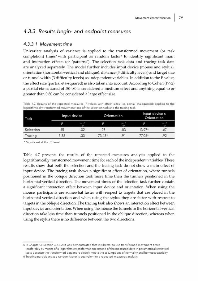
Movement characterization 79
4.3.3 Results begin- and endpoint measures
4.3.3.1 Movement timeUnivariate analysis of variance is applied to the transformed movement (or task completion) times5 with participant as random factor6 to identify significant main and interaction effects (or ‘patterns’). The selection task data and tracing task data are analyzed separately. The model further includes input device (mouse and stylus), orientation (horizontal-vertical and oblique), distance (3 difficulty levels) and target size or tunnel width (3 difficulty levels) as independent variables. In addition to the F-value, the effect size (partial eta-squared) is also taken into account. According to Cohen (1992) a partial eta-squared of .50-.80 is considered a medium effect and anything equal to or greater than 0.80 can be considered a large effect size.
Table 4.7. Results of the repeated measures (F-values with effect sizes, i.e. partial eta-squared) applied to the logarithmically transformed movement time of the selection task and the tracing task.
TaskInput device Orientation Input device x
Orientation
F ηp2 F ηp
2 F ηp2
Selection .15 .02 .25 .03 13.97* .67
Tracing 3.38 .33 73.43* .91 77.05* .92
* Significant at the .01 level
Table 4.7 presents the results of the repeated measures analysis applied to the logarithmically transformed movement time for each of the independent variables. These results show that both the selection and the tracing task do not show a main effect of input device. The tracing task shows a significant effect of orientation, where tunnels positioned in the oblique direction took more time than the tunnels positioned in the horizontal-vertical direction. The movement times of the selection task further contain a significant interaction effect between input device and orientation. When using the mouse, participants are somewhat faster with respect to targets that are placed in the horizontal-vertical direction and when using the stylus they are faster with respect to targets in the oblique direction. The tracing task also shows an interaction effect between input device and orientation. When using the mouse the tunnels in the horizontal-vertical direction take less time than tunnels positioned in the oblique direction, whereas when using the stylus there is no difference between the two directions.
5 In Chapter 3 (Section 3.2.3.2) it was demonstrated that it is better to use transformed movement times (preferably by means of a logarithmic transformation) instead of the measured data in parametrical statistical tests because the transformed data more closely meets the assumptions of normality and homoscedasticity.
6 Treating participant as a random factor is equivalent to a repeated-measures analysis
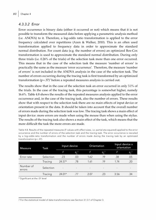
Chapter 480
4.3.3.2 ErrorError occurrence is binary data (either it occurred or not) which means that it is not possible to transform the measured data before applying a parametric analysis method (i.e. ANOVA) to it. Therefore, a log-odds ratio transformation is applied to the error frequency calculated over repetitions (Azen & Walker, 2010). This is an often used transformation applied to frequency data in order to approximate the standard normal distribution. For count data (e.g. the number of errors) an optimized Box-Cox transformation is used to approximate the standard normal distribution. During only three trials (i.e. 0.26% of the trials) of the selection task more than one error occurred. This means that in the case of the selection task the measure ‘number of errors’ is practically the same as the measure ‘error occurrence’. Therefore, the measure ‘number of errors’ is not included in the ANOVA analysis in the case of the selection task. The number of errors occurring during the tracing task is first transformed by an optimized transformation (p=.37)7 before a repeated measures analysis is carried out.
The results show that in the case of the selection task an error occurred in only 3.1% of the trials. In the case of the tracing task, this percentage is somewhat higher, namely 16.6%. Table 4.8 shows the results of the repeated measures analysis applied to the error occurrence and, in the case of the tracing task, also the number of errors. These results show that with respect to the selection task there are no main effects of input device or orientation present in the data. It should be taken into account that the overall number of errors made during the selection task was low. The tracing task shows a main effect of input device: more errors are made when using the mouse than when using the stylus. The results of the tracing task also shows a main effect of the task, which means that the more difficult the task the more errors are made.
Table 4.8. Results of the repeated measures (F-values with effect sizes, i.e. partial eta-squared) applied to the error occurrence and the number of errors of the selection task and the tracing task. The error occurrence is rescaled by a log-odds-ratio transformation and the number of errors made during the tracing task by an optimized transformation (p=.37).
Measure TaskInput device Orientation Input device x
orientation
F ηp2 F ηp
2 F ηp2
Error rate Selection .23 .03 1.62 .19 .38 .05
Tracing 24.57* .78 1.61 .19 1.74 .20
Number of errors Selection - - - - - -
Tracing 24.01* .77 2.07 .23 3.56 .34
* Significant at the .01 level
7 For the statistical model of data transformations see Section 3.1.3.1 of Chapter 3.

Movement characterization 81
As mentioned before, the percentage of trials in which an error was made during the selection and tracing task was fairly low: 3.1% and 16.6% of the trials, respectively. Since the measure of error magnitude only contains a value when an error occurs, this measure does not contain a proficient amount of information (i.e. has too many missing values) to discriminate between the various conditions in the case of the selection task. Therefore, the measure ‘error magnitude’ is not considered useful to quantify the quality of movements made in the current study.
In some studies movement time and error are the only quantitative measures used to determine which input device or interaction technique performs best (see for example Ahlström, 2005; Huff et al., 2006; MacKenzie, Sellen, & Buxton, 1991; Ware & Balakrishnan, 1994). Based on the analysis of the time and error measures of the current study one of the conclusions would be that, there is hardly any difference in performance between the mouse and the stylus especially in the case of the selection task. Although the mouse is equally fast (or slow) as the stylus, the movements might differ with respect to efficiency (with respect to path length and speed). This will be further explored in the next sections.
4.3.4 Results position-based measuresIn order to determine the complementary aspects captured by the position-based measures, a recursive clustering analysis is carried out. Before applying the clustering analysis all measures are transformed by a separately optimized Box-Cox transformation8. These transformations are implemented to achieve that all transformed measures are approximately normally distributed. For the derivation of the clusters an eigenvalue boundary of 1 is used9.
4.3.4.1 Selection taskIn Section 4.1.2 several measures are summed up to describe the traveled path. After deriving these measures from the selection task data a first check reveals that some of these position-based measures are not very useful to describe selection movements. In the selection task an overshoot occurred only in 32% of the trials. As a result, the measures ‘overshoot time’ and ‘percentage of maximum overshoot’ do not contain enough values (i.e. have too many missing values) for parametric analysis and will not be included in the clustering analysis.
8 See Figure 3.1 in Section 3.1.3.1 of Chapter 3 for the transformation model.9 An eigenvalue boundary of 1 prevents the creation of a cluster that contains only a single item (i.e. the identified
clusters will always consist of 2 or more measures).

Chapter 482
Table 4.9. Clustering of the measures according to the patterns identified with the 1D recursive clustering analysis of the begin- and endpoint measures and position-based measures applied to the selection task data.
Cluster A1 (Cronbach’s Alpha = .90)
Cluster A2(Cronbach’s Alpha = .84)
Measure R P Measure R P
Movement error .95 .09 Overshoot occurrence .93 .10
Movement variability .93 .10 Path length efficiency .87 .12
Movement offset .91 .11 High curvature analysis .84 .14
Task axis crossing .85 .12 Final positioning time .65 .18
Movement direction change .81 .14
Path length .70 .27
Target re-entry .33 .30
Cluster A3(Cronbach’s Alpha = .77)
Measure R P
Movement time .85 .14
Orthogonal direction change .82 .11
Error rate .81 .26
The recursive clustering analysis reveals three clusters within the time, error and position-based measures derived from the selection task data. Table 4.9 shows the separate clusters of measures together with the Cronbach’s Alpha, the correlations of the measures with the corresponding pattern (R-values) and the corresponding P-values. The Cronsbach’s Alpha is larger than .70 for all three clusters, indicating that the measures in each cluster have a good internal consistency and can reveal a similar pattern in the data. Although the first cluster has a high Cronbach’s Alpha, the measure ‘target re-entry’ has a low correlation (R=.33) with the corresponding pattern. This means that the measure of ‘target re-entry’ does not really fit within this cluster and does not correspond to any of the identified patterns. Since there is only one measure with such a low correlation, the recursive clustering algorithm didn’t see a need to create an additional cluster.
The clustering analysis shows that the time and error measures are clustered together (in cluster A3), which means that the other two clusters contain only position-based measures. This clearly shows that the position-based measures are able to reveal different patterns in the data than the time and error measures. This means that the position-based measures are indeed complementary to the time and error measures and can assist in gathering additional insights with respect to the executed movements.
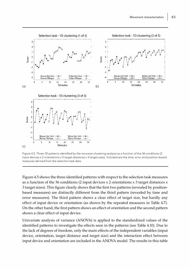
Movement characterization 83
(a) (b)
(c)
Figure 4.5. Three 1D patterns identified by the recursive clustering analysis as a function of the 36 conditions (2 input devices x 2 orientations x 3 target distances x 3 target sizes). Included are the time, error and position-based measures derived from the selection task data.
Figure 4.5 shows the three identified patterns with respect to the selection task measures as a function of the 36 conditions (2 input devices x 2 orientations x 3 target distances x 3 target sizes). This figure clearly shows that the first two patterns (revealed by position-based measures) are distinctly different from the third pattern (revealed by time and error measures). The third pattern shows a clear effect of target size, but hardly any effect of input device or orientation (as shown by the repeated measures in Table 4.7). On the other hand, the first pattern shows an effect of orientation and the second pattern shows a clear effect of input device.
Univariate analysis of variance (ANOVA) is applied to the standardized values of the identified patterns to investigate the effects seen in the patterns (see Table 4.10). Due to the lack of degrees of freedom, only the main effects of the independent variables (input device, orientation, target distance and target size) and the interaction effect between input device and orientation are included in the ANOVA model. The results in this table

Chapter 484
confirm the effects seen in Figure 4.5, but also reveal additional main and interaction effects. The first pattern does not only reveal a strong effect of orientation but also a highly significant main effect of distance and an interaction effect between input device and orientation. The second pattern does not only show a strong main effect of input device, but also of target size. The third pattern shows a highly significant main effect of distance and target size and only a small effect of input device.
Table 4.10. Results of the ANOVA (F-values and effect sizes, i.e. partial eta-squared) applied to the identified patterns within the begin- and endpoint measures and position-based measures derived from the selection task data (see Figure 4.5). To emphasize the larger effects, results with an effect size <.30 are greyed out.
PatternInput device Orientation Device x
orientationTarget
distance Target size
F ηp2 F ηp
2 F ηp2 F ηp
2 F ηp2
1 2.11 .07 174.84** .86 126.38** .82 161.38** .92 6.60** .32
2 236.03** .89 5.90* .17 .18 .01 1.66 .11 53.52** .79
3 5.26* .16 .04 .00 3.04 .10 28.01** .67 70.13** .83
* Significant at the .05 level** Significant at the .01 level
4.3.4.2 Tracing task
Table 4.11. Clustering of the measures according to the patterns identified with the 1D recursive clustering analysis of the begin- and endpoint measures and position-based measures applied to the tracing task data.
Cluster A1(Cronbach’s Alpha = .86)
Cluster A2(Cronbach’s Alpha = .84)
Measure R P Measure R P
Movement direction change .93 .08 Movement error .98 .04
Movement time .92 .09 Movement offset .92 .09
Task axis crossing .86 .12 Movement variability .90 .10
Path length .80 .24 Final positioning time .46 .25
Path length efficiency .48 .19
Cluster A3(Cronbach’s Alpha = .85)
Measure R P
Error rate .94 .08
Number of errors .93 .08
Orthogonal direction change .78 .17
High curvature analysis .66 .20

Movement characterization 85
Also in the case of the tracing task a first check of the derived measures reveals that some of these position-based measures are not very useful to describe tracing movements. During the tracing task an overshoot occurs in only 9 trials (i.e. 0.78% of the trials) and a target re-entry occurs in only 3 trials (i.e. 0.26% of the trials). This means that there is no information contained in the measures ‘target re-entry’, ‘overshoot occurrence’, ‘overshoot time’ and ‘percentage of maximum overshoot’. These measures will therefore not be included in the clustering analysis.
Table 4.11 shows the results of the recursive clustering analysis of the time, error and position-based measures applied to the tracing task data. This table shows three clusters with Cronbach’s Alpha larger than .80. The correlations show that two measures do not really fit within the identified clusters, namely the final positioning time (R=.46) and path length efficiency (R=.48). In contrast to the selection task, the time and error measures of the tracing task are not part of the same cluster, but of two separate clusters. This means that the begin- and endpoint measures are able to reveal two different kind of patterns in the data. The other pattern is revealed by several position-based measures, indicating that also in the case of the tracing task the position-based measures can be of added value.
(a) (b)
(c)
Figure 4.6. Three 1D patterns identified by recursive clustering analysis as a function of the 36 conditions (2 input devices x 2 orientations x 3 tunnel lengths x 3 tunnel widths). Included are the time, error and position-based measures derived from the tracing task data.
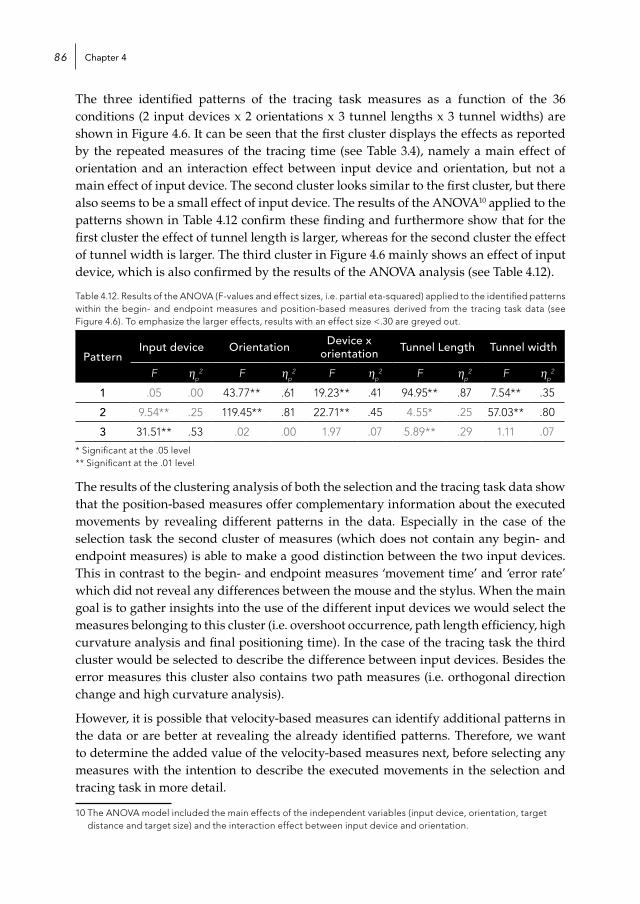
Chapter 486
The three identified patterns of the tracing task measures as a function of the 36 conditions (2 input devices x 2 orientations x 3 tunnel lengths x 3 tunnel widths) are shown in Figure 4.6. It can be seen that the first cluster displays the effects as reported by the repeated measures of the tracing time (see Table 3.4), namely a main effect of orientation and an interaction effect between input device and orientation, but not a main effect of input device. The second cluster looks similar to the first cluster, but there also seems to be a small effect of input device. The results of the ANOVA10 applied to the patterns shown in Table 4.12 confirm these finding and furthermore show that for the first cluster the effect of tunnel length is larger, whereas for the second cluster the effect of tunnel width is larger. The third cluster in Figure 4.6 mainly shows an effect of input device, which is also confirmed by the results of the ANOVA analysis (see Table 4.12).
Table 4.12. Results of the ANOVA (F-values and effect sizes, i.e. partial eta-squared) applied to the identified patterns within the begin- and endpoint measures and position-based measures derived from the tracing task data (see Figure 4.6). To emphasize the larger effects, results with an effect size <.30 are greyed out.
PatternInput device Orientation Device x
orientation Tunnel Length Tunnel width
F ηp2 F ηp
2 F ηp2 F ηp
2 F ηp2
1 .05 .00 43.77** .61 19.23** .41 94.95** .87 7.54** .35
2 9.54** .25 119.45** .81 22.71** .45 4.55* .25 57.03** .80
3 31.51** .53 .02 .00 1.97 .07 5.89** .29 1.11 .07
* Significant at the .05 level** Significant at the .01 level
The results of the clustering analysis of both the selection and the tracing task data show that the position-based measures offer complementary information about the executed movements by revealing different patterns in the data. Especially in the case of the selection task the second cluster of measures (which does not contain any begin- and endpoint measures) is able to make a good distinction between the two input devices. This in contrast to the begin- and endpoint measures ‘movement time’ and ‘error rate’ which did not reveal any differences between the mouse and the stylus. When the main goal is to gather insights into the use of the different input devices we would select the measures belonging to this cluster (i.e. overshoot occurrence, path length efficiency, high curvature analysis and final positioning time). In the case of the tracing task the third cluster would be selected to describe the difference between input devices. Besides the error measures this cluster also contains two path measures (i.e. orthogonal direction change and high curvature analysis).
However, it is possible that velocity-based measures can identify additional patterns in the data or are better at revealing the already identified patterns. Therefore, we want to determine the added value of the velocity-based measures next, before selecting any measures with the intention to describe the executed movements in the selection and tracing task in more detail.
10 The ANOVA model included the main effects of the independent variables (input device, orientation, target distance and target size) and the interaction effect between input device and orientation.

Movement characterization 87
4.3.5 Results velocity-based measuresIn order to determine the added value of the velocity-based measures, these measures are added to the time, error and position-based measures in the recursive clustering analysis. Before applying the clustering analysis these velocity-based measures are also transformed by a separately optimized Box-Cox transformation. These transformations are implemented to achieve that the transformed measures are normally distributed. For the derivation of the clusters again an eigenvalue boundary of 1 is used11.
4.3.5.1 Selection taskTable 4.13. Clustering of the measures according to the patterns identified with the 1D recursive clustering analysis of the begin- and endpoint measures, position-based measures and velocity-based measures applied to the selection task data.
Cluster B1(Cronbach’s Alpha = .96)
Cluster B2(Cronbach’s Alpha = .91)
Measure R P Measure R P
Relative time to peak speed .97 .09 Acceleration time .96 .07
Time to peak speed .96 .10 Deceleration time .94 .08
Number of type-3 submovements .96 .10 Movement direction change .94 .08
Number of submovements .91 .12 Movement time .86 .13
Peak deceleration .87 .16 Task axis crossing .83 .12
Peak acceleration .85 .17 Number of type-2 submovements .81 .15
Final positioning time .84 .13 Orthogonal direction change .61 .15
Path length efficiency .71 .17 Target re-entry .34 .30
Cluster B3(Cronbach’s Alpha = .91)
Cluster B4(Cronbach’s Alpha = .99)
Measure R P Measure R P
Number of type-1 submovements .91 .11 Movement error 1.00 .02
High curvature analysis .91 .11 Movement variability .98 .05
Overshoot occurrence .86 .14 Movement offset .98 .05
Number of pauses .85 .09
Pause occurrence .85 .09
Error rate .60 .36
Cluster B5(Cronbach’s Alpha = .94)
Measure R P
Path length .96 .10
Average speed .96 .08
Peak speed .91 .13
11 An eigenvalue boundary of 1 prevents the creation of a cluster that contains only a single item (i.e. the identified clusters will always consist of 2 or more measures).
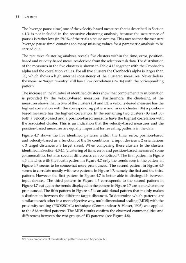
Chapter 488
The ‘average pause time’, one of the velocity-based measures that is described in Section 4.1.3, is not included in the recursive clustering analysis, because the occurrence of pauses is rather low (in 29.0% of the trials a pause occurs). This means that the measure ‘average pause time’ contains too many missing values for a parametric analysis to be carried out.
The recursive clustering analysis reveals five clusters within the time, error, position-based and velocity-based measures derived from the selection task data. The distribution of the measures in the five clusters is shown in Table 4.13 together with the Cronbach’s alpha and the correlation values. For all five clusters the Cronbach’s alpha is larger than .90, which shows a high internal consistency of the clustered measures. Nevertheless, the measure ‘target re-entry’ still has a low correlation (R=.34) with the corresponding pattern.
The increase in the number of identified clusters show that complementary information is provided by the velocity-based measures. Furthermore, the clustering of the measures shows that in two of the clusters (B1 and B2) a velocity-based measure has the highest correlation with the corresponding pattern and in one cluster (B4) a position-based measure has the highest correlation. In the remaining two clusters (B3 and B5) both a velocity-based and a position-based measure have the highest correlation with the associated cluster. This is an indication that the velocity-based measures and the position-based measures are equally important for revealing patterns in the data.
Figure 4.7 shows the five identified patterns within the time, error, position-based and velocity-based as a function of the 36 conditions (2 input devices x 2 orientations x 3 target distances x 3 target sizes). When comparing these clusters to the clusters identified in Section 4.3.4.1 (clustering of time, error and position-based measures) some commonalities but also several differences can be noticed12. The first pattern in Figure 4.5 matches with the fourth pattern in Figure 4.7, only the trends seen in the pattern in Figure 4.7 seems to be somewhat more pronounced. The second pattern in Figure 4.5 seems to correlate mostly with two patterns in Figure 4.7, namely the first and the third pattern. However the first pattern in Figure 4.7 is better able to distinguish between input devices. The third pattern in Figure 4.5 corresponds to the second pattern in Figure 4.7 but again the trends displayed in the pattern in Figure 4.7 are somewhat more pronounced. The fifth pattern in Figure 4.7 is an additional pattern that mainly makes a distinction between the different target distances. To determine which patterns are similar to each other in a more objective way, multidimensional scaling (MDS) with the proximity scaling (PROXSCAL) technique (Commandeur & Heiser, 1993) was applied to the 8 identified patterns. The MDS results confirm the observed commonalities and differences between the two groups of 1D patterns (see Figure 4.8).12
12 For a comparison of the identified patterns see also Appendix A.2.

Movement characterization 89
(a) (b)
(c) (d)
(e)
Figure 4.7. Five 1D patterns identified by recursive clustering analysis as a function of the 36 conditions (2 input devices x 2 orientations x 3 target distances x 3 target sizes). Included are the time, error, position-based and velocity-based measures derived from the selection task data.
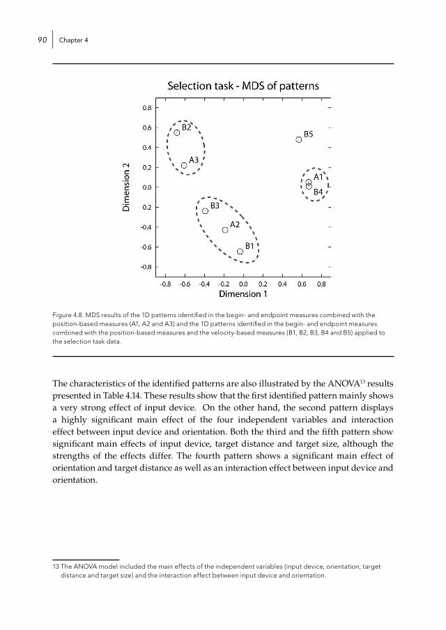
Chapter 490
Figure 4.8. MDS results of the 1D patterns identified in the begin- and endpoint measures combined with the position-based measures (A1, A2 and A3) and the 1D patterns identified in the begin- and endpoint measures combined with the position-based measures and the velocity-based measures (B1, B2, B3, B4 and B5) applied to the selection task data.
The characteristics of the identified patterns are also illustrated by the ANOVA13 results presented in Table 4.14. These results show that the first identified pattern mainly shows a very strong effect of input device. On the other hand, the second pattern displays a highly significant main effect of the four independent variables and interaction effect between input device and orientation. Both the third and the fifth pattern show significant main effects of input device, target distance and target size, although the strengths of the effects differ. The fourth pattern shows a significant main effect of orientation and target distance as well as an interaction effect between input device and orientation.
13 The ANOVA model included the main effects of the independent variables (input device, orientation, target distance and target size) and the interaction effect between input device and orientation.

Movement characterization 91
Table 4.14. Results of the ANOVA (F-values and effect sizes, i.e. partial eta-squared) applied to the identified patterns in the begin- and endpoint measures, position-based measures and velocity-based measures derived from the selection task data (see Figure 4.7). To emphasize the larger effects, results with an effect size <.30 are greyed out.
PatternInput device Orientation Device x
orientationTarget
distance Target size
F ηp2 F ηp
2 F ηp2 F ηp
2 F ηp2
1 1410.30** .98 .85 .03 2.98 .10 2.23 .14 1.23 .08
2 111.08** .80 53.08** .66 50.95** .65 156.77** .92 87.80** .86
3 88.96** .76 7.14* .20 9.55** .25 9.94** .40 91.07** .87
4 10.11** .27 101.49** .78 86.83** .76 52.93** .79 .44 .03
5 260.29** .90 3.53 .11 7.20* .21 1945.21** .99 15.87** .53
* Significant at the .05 level** Significant at the .01 level
4.3.5.2 Tracing taskA trial during the tracing task rarely contains more than one pause (only in 0.35% of the trials). This means that the measure ‘number of pause’ contains almost the same information as the measure ‘pause occurrence’. Furthermore, a pause is identified in only 6.3% of the trials, which means that the measure ‘pause time’ contains too many missing values for parametric analysis. The number of pauses and pause time are therefore not included in the clustering analysis.
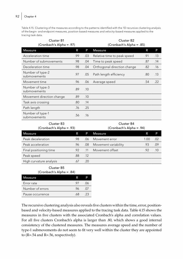
Chapter 492
Table 4.15. Clustering of the measures according to the patterns identified with the 1D recursive clustering analysis of the begin- and endpoint measures, position-based measures and velocity-based measures applied to the tracing task data.
Cluster B1(Cronbach’s Alpha = .97)
Cluster B2(Cronbach’s Alpha = .85)
Measure R P Measure R P
Acceleration time .99 .03 Relative time to peak speed .91 .13
Number of submovements .98 .04 Time to peak speed .87 .14
Deceleration time .98 .04 Orthogonal direction change .82 .16
Number of type-2 submovements .97 .05 Path length efficiency .80 .13
Movement time .96 .06 Average speed .54 .22
Number of type-3 submovements .89 .10
Movement direction change .89 .10
Task axis crossing .80 .14
Path length .76 .25
Number of type-1 submovements .56 .16
Cluster B3(Cronbach’s Alpha = .93)
Cluster B4(Cronbach’s Alpha = .94)
Measure R P Measure R P
Peak deceleration .98 .06 Movement error 1.00 .02
Peak acceleration .96 .08 Movement variability .93 .09
Final positioning time .92 .11 Movement offset .92 .10
Peak speed .88 .12
High curvature analysis .67 .20
Cluster B5(Cronbach’s Alpha = .84)
Measure R P
Error rate .97 .06
Number of errors .96 .07
Pause occurrence .68 .23
The recursive clustering analysis also reveals five clusters within the time, error, position-based and velocity-based measures applied to the tracing task data. Table 4.15 shows the measures in five clusters with the associated Cronbach’s alpha and correlation values. For all five clusters Cronbach’s alpha is larger than .80, which shows a good internal consistency of the clustered measures. The measures average speed and the number of type-1 submovements do not seem to fit very well within the cluster they are appointed to (R=.54 and R=.56, respectively).
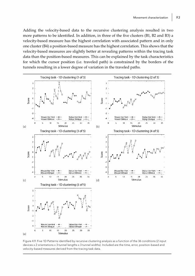
Movement characterization 93
Adding the velocity-based data to the recursive clustering analysis resulted in two more patterns to be identified. In addition, in three of the five clusters (B1, B2 and B3) a velocity-based measure has the highest correlation with associated pattern and in only one cluster (B4) a position-based measure has the highest correlation. This shows that the velocity-based measures are slightly better at revealing patterns within the tracing task data than the position-based measures. This can be explained by the task characteristics for which the cursor position (i.e. traveled path) is constrained by the borders of the tunnels resulting in a lower degree of variation in the traveled paths.
(a) (b)
(c) (d)
(e)
Figure 4.9. Five 1D Patterns identified by recursive clustering analysis as a function of the 36 conditions (2 input devices x 2 orientations x 3 tunnel lengths x 3 tunnel widths). Included are the time, error, position-based and velocity-based measures derived from the tracing task data.

Chapter 494
The three patterns identified within the time, error and position-based measures (see Figure 4.6) are similar to three of the five patterns identified within the time, error, position-based and velocity-based measures (see Figure 4.9)14. This means that the two other patterns (B2 and B3) are able to reveal two new patterns within the tracing task data. The observations with respect to the commonalities and dissimilarities between the two groups of 1D patterns are confirmed by the MDS (PROXSCAL) analysis applied to the 8 identified patterns (see Figure 4.10).
Figure 4.10. MDS results of the 1D patterns identified within the begin- and endpoint measures combined with the position-based measures (A1, A2 and A3) and the 1D patterns identified within the begin- and endpoint measures combined with the position-based measures and the velocity-based measures (B1, B2, B3, B4 and B5) applied to the tracing task data.
The characteristics of the identified patterns are also illustrated by the results of the ANOVA analysis15 presented in Table 4.16. These results show that the two additional patterns display a strong effect of input device. The second pattern also shows an effect of tunnel length. The third pattern shows a significant effect of the four independent
14 The first pattern in Figure 4.6 corresponds to the first pattern in Figure 4.9, the second pattern in Figure 4.6 corresponds to the fourth pattern in Figure 4.9 and the third pattern in Figure 4.6 corresponds to the fifth pattern in Figure 4.9. For a comparison of the identified patterns see also Appendix A.3.
15 The ANOVA model included the main effects of the independent variables (input device, orientation, target distance and target size) and the interaction effect between input device and orientation.

Movement characterization 95
variables (with the strongest effect of input device) and an interaction effect between input device and orientation.
Table 4.16. Results of the ANOVA (F-values and effect sizes, i.e. partial eta-squared) applied to the identified patterns within the begin- and endpoint measures, position-based measures and velocity-based measures derived from the tracing task data (see Figure 4.9). To emphasize the larger effects, results with an effect size <.30 are greyed out.
PatternInput device Orientation Device x
orientation Tunnel length Tunnel width
F ηp2 F ηp
2 F ηp2 F ηp
2 F ηp2
1 .01 .00 21.03** .43 13.73** .33 65.75** .82 14.65 .51
2 287.28** .91 2.12 .07 .30 .01 23.62** .63 .62 .04
3 197.39** .88 26.88** .49 13.55** .33 14.58** .51 65.16** .82
4 1.62 .06 137.70** .83 24.65** .47 4.80* .26 39.95** .74
5 14.21** .34 .02 .00 3.17 .10 4.15* .23 1.71 .11
* Significant at the .05 level** Significant at the .01 level
The recursive clustering analysis shows that adding the velocity-based measures mainly results in the identification of one or more patterns that are better able to discriminate between input devices. This is the case for the measures derived from the selection task data as well as for the measures derived from the tracing task data. These findings are confirmed by the 2D clustering of the identified patterns shown in Figure 4.11 and Figure 4.12 for the selection task and the tracing task, respectively.
Figure 4.11a and Figure 4.12a show the 2D clustering of the identified patterns in the time, error and position-based measures of the selection task and the tracing task, respectively. Figure 4.11b and Figure 4.12b show the 2D clustering when the velocity-based measures are also included in the clustering analysis of the selection task and the tracing task, respectively. Besides the direction of the identified patterns also the distribution of the 36 conditions (2 input devices x 2 orientations x 3 target distances x 3 target sizes) are displayed in these figures. These distributions show that for both the selection and the tracing task the addition of the velocity-based measures enables a better discrimination between the conditions of the different input devices. In Figure 4.11b and Figure 4.12b the conditions corresponding to the different input devices and orientations are better grouped together (especially with respect to the different input devices) than the conditions displayed in Figure 4.11a and Figure 4.12a.

Chapter 496
(a) (b)
Figure 4.11. 2D clustering of the identified 1D patterns in the selection task data with: a) begin- and endpoint measures and position-based measures; b) begin- and endpoint measures, position-based measures and velocity-based measures. The length of the vectors indicates the amount of variation explained.
(a) (b)
Figure 4.12. 2D clustering of the identified 1D patterns in the tracing task data with: a) begin- and endpoint measures and position-based measures; b) begin- and endpoint measures, position-based measures and velocity-based measures. The length of the vectors indicates the amount of variation explained.

Movement characterization 97
4.3.6 Results measure selectionAs shown in Paragraph 4.3.3.1 movement time does not reveal a difference between input devices in both the selection task and the tracing task. This means that measures selected with multiple regression analysis will also not reveal any differences between input devices. We believe that the selection method based on recursive clustering analysis can help in gathering more insights into the differences between input devices (as described in Paragraph 4.2.3).
4.3.6.1 Selection taskThe results of the ANOVA analysis applied to the identified patterns within the measures derived from the selection task data showed that one cluster of measures (cluster B1) is highly capable of making a distinction between input devices. This cluster includes measures such as (relative) time to peak speed, number of (type-3) submovements, peak deceleration and acceleration, final positioning time and path length efficiency. Although the other patterns are also able to make a distinction between input devices, the measures of the selected cluster (B1) will reveal larger and therefore more important differences between the input devices (except maybe for path efficiency, which has a somewhat lower correlation with the pattern).
Table 4.17. Results of the repeated measures (F-values with effect sizes, i.e. partial eta-squared) applied to selection of measures derived from the selection task data. Results that are not significant (p>.05) are greyed out.
MeasureInput device Device x
orientation
Device xtarget
distance
Device xtarget size
F ηp2 F ηp
2 F ηp2 F ηp
2
Final positioning time 193.09** .96 .35 .02 .38 .04 3.35 .32
Relative time to peak speed 147.66** .96 1.32 .16 2.25 .24 1.45 .17
Time to peak speed 137.07** .95 .41 .06 11.12** .61 .26 .04
Number of type-3 submovements 121.19** .95 11.20* .62 9.15** .57 .26 .04
Number of submovements 96.36** .93 22.34** .76 10.85** .61 1.01 .13
Peak acceleration 78.41** .92 13.39** .66 1.40 .17 1.22 .15
Peak deceleration 76.97** .92 9.68* .58 1.23 .15 1.78 .20
Path length efficiency 13.70** .66 3.88 .36 .19 .03 .22 .03
* Significant at the .05 level** Significant at the .01 level
In Table 4.17 the results are presented of the repeated measures analysis applied to the measures which are selected to describe the difference between the input devices in the case of the selection task. These results show that with respect to selection movements the largest difference between the mouse and the stylus can be noticed in the final

Chapter 498
positioning time, i.e. the time to select a target once the cursor has (last) entered the target. This positioning time is longer for the mouse than for the stylus. This means that keeping the cursor on target and pressing the button to select the target is more difficult when using the mouse than when using the stylus.
With respect to the movement towards the target, the movements made with the mouse sooner reach the peak speed, also relatively to the total movement time (in the latter case the difference between the input devices is even larger). In addition, the peak deceleration and acceleration is higher for mouse movements. This can be explained by the control-to-display ratio (1:4) of the mouse compared to that of the stylus (1:1), which enables users to move faster with the mouse and sooner reaching the peak speed with a higher acceleration rate.
Furthermore, movements made with the stylus contain more submovements, especially type-3 submovements, which are considered to be subtle accuracy regulations. In addition, the path length efficiency is also higher, which means that although selection movements with the stylus are slower, they are more often subtly corrected along the way, which makes them more efficient with respect to the traveled path.
4.3.6.2 Tracing taskThe results of the ANOVA analysis applied to the identified patterns within the measures derived from the tracing task data showed that two clusters of measures (cluster B2 and cluster B3) are best able to make a distinction between the mouse and the stylus. Measures loading high on the second pattern include (relative) time to peak speed, orthogonal direction change and path length efficiency. Measures loading high on the third pattern are peak deceleration and acceleration, final positioning time and peak speed. Since average speed and high curvature analysis have a low correlation with the corresponding pattern, we decided not to include these measures in the selection.
Table 4.18 shows the results of the repeated measures analysis applied to the measures which are selected to describe the difference between the input devices in the case of the tracing task. These results show that with respect to tunnel tracing the largest difference between the input devices is revealed by the time at which the peak speed is reached: movements with the mouse reach their peak speed sooner, also relatively to the total movement time (in the latter case the difference between the input devices is even larger). Furthermore, the peak acceleration, peak deceleration and peak speed are higher when using the mouse than when using the stylus. Again, this can be explained by the different control-to-display ratio of the mouse and the stylus.

Movement characterization 99
Table 4.18. Results of the repeated measures (F-values with effect sizes, i.e. partial eta-squared) applied to selection of measures derived from the tracing task data. Results that are not significant (p>.05) are greyed out.
MeasureInput device Device x
orientationDevice x
tunnel lengthDevice x
tunnel width
F ηp2 F ηp
2 F ηp2 F ηp
2
Relative time to peak speed 91.41** .93 .07 .01 .75 .10 5.72* .45
Orthogonal direction change 72.67** .91 .01 .00 .01 .00 1.03 .13
Peak acceleration 34.92** .83 43.11** .86 1.38 .17 22.59** .76
Path length efficiency 32.44** .82 1.42 .17 6.40* .48 9.55** .58
Peak deceleration 31.38** .82 24.96** .78 .20 .03 16.26** .70
Time to peak speed 27.96** .80 2.41 .26 1.80 .21 19.87** .74
Final positioning time 10.25* .59 1.65 .19 1.55 .18 2.37 .25
Peak speed 5.23* .43 45.51** .87 13.48** .66 48.03** .87
* Significant at the .05 level** Significant at the .01 level
In contrast to the selection task the path length efficiency of movements made with the mouse is higher than that of the movements made with the stylus. In the case of the mouse the mean path efficiency value was lower than 1, which means that participants often did not continue to the center of the target area but ended the movement as soon as the target border was crossed. Another explanation is that with the stylus more orthogonal direction changes were made, which makes the movement less efficient. Finally, the final positioning time was longer when the mouse was used than when the stylus was used, which can be an indication that the motion termination is more difficult when using the mouse than when using the stylus.
4.4 Conclusion & discussionThe main goal of this chapter was not to propose a selection of measures that we think should be used in the evaluation of input devices and interaction techniques. As was already acknowledged by MacKenzie et al. (2001) the importance of certain measures can simply reflect a particular device and/or task. Therefore, we only wanted to support the selection process by providing insights into the possible added value of more complex measures and by proposing a selection procedure that was more aimed at addressing a specific question such as distinguishing between two input devices. Below we will describe and discuss the conclusions with respect to the questions posed in Section 4.3.1.
Are more complex measures, that require more effort with respect to data logging and computation, able to capture additional aspects of movement quality besides the aspects already captured by the time and error measures in the case of the selection task and the tracing task?
In other words, do the benefits of having more complex measures to describe movement

Chapter 4100
quality outweigh the costs of deriving these measures from the data? We believe they do. The analysis of the begin-and end-point measures showed that movement time did not reveal any difference between input devices in neither the selection nor the tracing task and the error measures only showed a significant difference between input devices in the tracing task. The cluster analysis including the begin- and endpoint measures and the position-based measures showed that besides the patterns including the time and error measures additional patterns were identified. In the case of the selection task, one of the additional patterns (not containing begin- and endpoint measures) was very capable to make a distinction between the two input devices. In the case of the tracing task, several position-based measures were clustered with the error measures and were also able to differentiate input devices from each other.
The inclusion of the velocity-based measures resulted in the identification of two additional patterns for both the selection and tracing task data. The increase in the number of identified clusters showed that complementary information was provided by the velocity-based measures. In addition, the inclusion of the velocity-based measures revealed patterns that were considerably better at making a distinction between the two input devices, especially in the case of the selection task. In this experimental setting the velocity-based measures were considered to be important for the description of the differences between the mouse and the stylus for both the selection task and the tracing task data.
In the case of the tracing task a velocity-based measure had the highest correlation with the corresponding pattern in three of the five clusters and a position-based measure had the highest correlation with the corresponding pattern in only one cluster. This suggested that it would be more beneficial to select velocity-based measures to describe the quality of tracing movement than position-based measures because they were slightly better at revealing patterns within the tracing task data. In the case of the tracing task data this could be the case, due to the task characteristics for which the cursor position was constrained by the borders of the tunnels resulting in a lower degree of variation in the traveled paths. However, in the case of the selection task data the degree to which the position-based and the velocity-based measures correlated with the corresponding patterns showed that both the velocity-based measures and the position-based measures were equally important for revealing patterns in the data. Therefore, we advise to select measures from all three groups of measures (begin- and endpoint, position-based and velocity-based measures) for gathering insights into movement quality.
What measures would be selected when we want to describe the differences in movement quality of the used input devices (mouse and stylus) in the case of the selection task and the tracing task?
The selection of measures to be used in an experiment has mainly been a subjective process that also largely depended on the system being tested. MacKenzie et al. (2001) acknowledged this in their conclusion that the importance of the measures target re-entry and movement offset in their study could simply reflect a particular device and/or

Movement characterization 101
task. In the introduction we proposed a different approach towards selecting measures which is more tailored to the question we would like to answer. For example, when designing input devices or interaction techniques we will be interested in measures that can best describe the differences between these input devices or interaction techniques. We showed that recursive clustering analysis could be well used to select measures based on the pattern (in our case the difference between input devices) that this cluster of measures was able to reveal.
The selection of measures resulted in a clear description of the main aspects in which the movements made with mouse and the stylus differed from each other. Of the eight selected measures six measures were the same for both the selection task and the tracing task: final positioning time, time and relative time to peak speed, peak acceleration and deceleration and path length efficiency. The difference between input devices used in the selection task could be further described by the number of submovements and the number of type-3 submovements. In the case of the tracing task the difference between input devices could also be described by the number of orthogonal direction changes and the peak speed of the movement.
- - -
Position-based measures and velocity based measures were able to provide a more detailed insight into the movement quality. In the next chapter we will explore whether or not it is beneficial to look at movements in even more detail by dividing them into movement phases.

Chapter 4102

Chapter 5
Movement phases

Chapter 5104
5.1 Division in movement phasesIn the previous chapter the movement quality was associated with features derived from the traveled path and the velocity and acceleration profile. However, it is possible to investigate aiming movements in even greater detail by dividing the movements into different phases. By characterizing the movement phases it is possible to pinpoint more precisely during what stage of the movement certain differences with respect to movement quality occur between for example input devices or interaction techniques. The idea of dividing movements into phases stems from early research into the characteristics of voluntary movements. Already in 1899, Robert Woodworth published a model of aimed movements that divides them into two components (Woodworth, 1899). According to this model, goal-directed movements consist of an initial impulse or ballistic phase and a perceptually guided final control or correction phase. The initial part of the movement is relatively fast, but as people get close to the target the movement becomes slower and is characterized by irregularities in the time-displacement profile.
According to Meyer, Abrams, Kornblum, Wright, & Smith (1988), the ballistic phase is programmed to reach the target, and the unintended errors are corrected during the correction phase using sensory feedback (see also Figure 4.3). Based on the two-component model, Meyer et al. (1988) proposed parsing criteria to indicate the end of the first submovement, or ballistic phase: a) a zero-crossing of the displacement velocity from positive to negative (type-1); b) a zero-crossing of the acceleration, which is the derivative of velocity, from negative to positive (type-2); c) a zero-crossing of jerk, which is the derivative of acceleration, from positive to negative (type-3). Recent comparative studies used these criteria to divide movements into submovements in order to look at movements in more detail (Hourcade, 2006; Hwang, Keates, Langdon, & Cohen, 2005; Wisleder & Dounskaia, 2007).
Although Woodworth’s model formed the basis for Meyer’s optimized dual-submovement model, the criteria that Meyer et al. (1988) proposed do not necessarily divide the movement into a ballistic phase and a correction phase. They assumed that goal-directed movements consisted of maximally two submovements and that the ballistic phase ends after the first submovement. If one examines the velocity profiles of goal-directed movements, one can observe that this is frequently not the case. For example, Figure 5.1a shows an example of a velocity profile of a goal-directed movement carried out with a mouse. This graph shows that not one but two large submovements were necessary to get into the neighborhood of the target. Another example is shown in Figure 5.1b, which demonstrates that subtle changes in the deceleration rate, also called type-3 submovements, can occur when using a stylus. According to Wisleder and Dounskaia (2007) type-3 submovements occur during relatively smooth motions and are only an indication of subtle accuracy regulation. In other words, they are not believed to signal actual interruptions in the ballistic movement and, therefore, they are not likely to indicate the end of the ballistic phase.
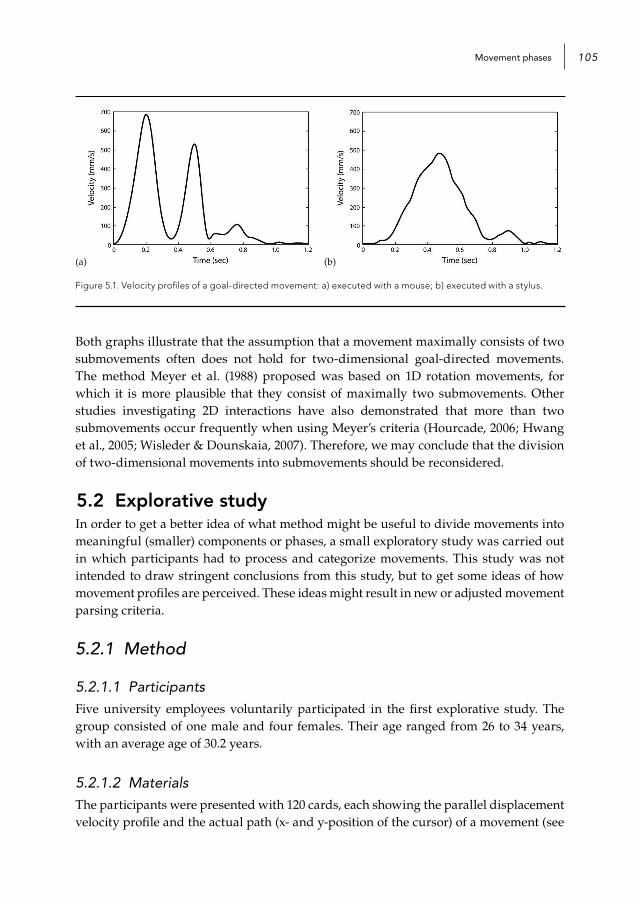
Movement phases 105
(a) (b)
Figure 5.1. Velocity profiles of a goal-directed movement: a) executed with a mouse; b) executed with a stylus.
Both graphs illustrate that the assumption that a movement maximally consists of two submovements often does not hold for two-dimensional goal-directed movements. The method Meyer et al. (1988) proposed was based on 1D rotation movements, for which it is more plausible that they consist of maximally two submovements. Other studies investigating 2D interactions have also demonstrated that more than two submovements occur frequently when using Meyer’s criteria (Hourcade, 2006; Hwang et al., 2005; Wisleder & Dounskaia, 2007). Therefore, we may conclude that the division of two-dimensional movements into submovements should be reconsidered.
5.2 Explorative studyIn order to get a better idea of what method might be useful to divide movements into meaningful (smaller) components or phases, a small exploratory study was carried out in which participants had to process and categorize movements. This study was not intended to draw stringent conclusions from this study, but to get some ideas of how movement profiles are perceived. These ideas might result in new or adjusted movement parsing criteria.
5.2.1 Method
5.2.1.1 ParticipantsFive university employees voluntarily participated in the first explorative study. The group consisted of one male and four females. Their age ranged from 26 to 34 years, with an average age of 30.2 years.
5.2.1.2 MaterialsThe participants were presented with 120 cards, each showing the parallel displacement velocity profile and the actual path (x- and y-position of the cursor) of a movement (see
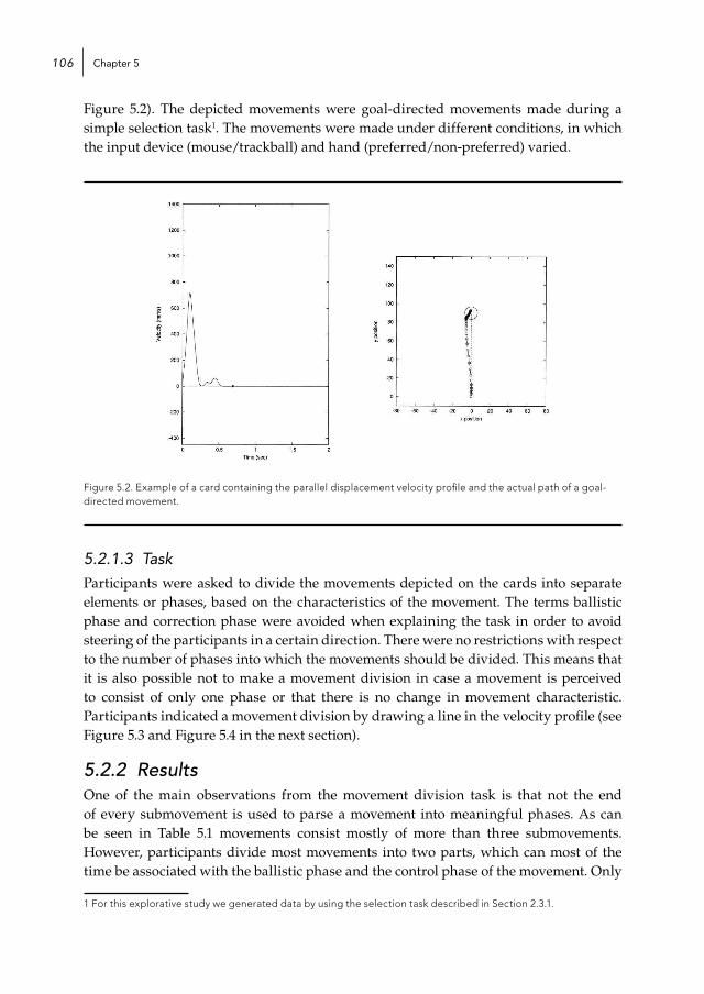
Chapter 5106
Figure 5.2). The depicted movements were goal-directed movements made during a simple selection task1. The movements were made under different conditions, in which the input device (mouse/trackball) and hand (preferred/non-preferred) varied.
Figure 5.2. Example of a card containing the parallel displacement velocity profile and the actual path of a goal-directed movement.
5.2.1.3 TaskParticipants were asked to divide the movements depicted on the cards into separate elements or phases, based on the characteristics of the movement. The terms ballistic phase and correction phase were avoided when explaining the task in order to avoid steering of the participants in a certain direction. There were no restrictions with respect to the number of phases into which the movements should be divided. This means that it is also possible not to make a movement division in case a movement is perceived to consist of only one phase or that there is no change in movement characteristic. Participants indicated a movement division by drawing a line in the velocity profile (see Figure 5.3 and Figure 5.4 in the next section).
5.2.2 Results One of the main observations from the movement division task is that not the end of every submovement is used to parse a movement into meaningful phases. As can be seen in Table 5.1 movements consist mostly of more than three submovements. However, participants divide most movements into two parts, which can most of the time be associated with the ballistic phase and the control phase of the movement. Only
1 For this explorative study we generated data by using the selection task described in Section 2.3.1.

Movement phases 107
one participant (pp 5) divides movements slightly more often into three parts than into two parts. This division into three parts often corresponds to the ballistic phase and a correction phase that consists of a phase in which large correction movements are made and a phase in which small correction movements (i.e. fine tuning) are made. This was also mentioned by participant 4 who tried to make a distinction between large correction movements and small correction movements..
Table 5.1. Percentage of movements divided into 1, 2, 3, 4, 5 or more than 5 parts by parsing software (PS)2 and the 5 participants (PP).
Number of elements
1 2 3 4 5 >5
PS 1.7 14.2 25.8 25 14.2 19.2
PP 1 33.3 50.0 15.8 0 0.8 0
PP 2 30.0 44.2 17.5 7.5 0.8 0
PP 3 0.8 92.5 6.7 0 0 0
PP 4 0.8 59.2 39.2 0.8 0 0
PP 5 2.5 40.0 40.8 12.5 4.2 0
Table 5.2 shows the mean number of submovements that occur before the first division indication. This table shows that participants do not systematically indicate the end of the first phase after the primary submovement, which, according to Meyer et al. (1988), is the criterion to divide a movement into its ballistic phase and correction phase. Especially when looking at the movements made with the trackball the first phase often contains several submovements.
Table 5.2. Mean number of submovements before first division indication by the 5 participants (PP) for input device (mouse / trackball) and hand of use (preferred hand / non-preferred hand).
PP
Number of submovements
Mouse Trackball
Pref. hand N-pref. hand Pref. hand N-pref. hand
1 2.4 2.0 2.7 2.6
2 2.4 1.8 3.1 2.6
3 1.7 1.5 2.0 1.4
4 1.4 1.1 1.7 1.4
5 1.4 1.2 1.9 1.3
The divisions participants made are identified as type-1, type-2 or type-3 submovements, where type-1 movements do not only indicate overshoots with a velocity zero-crossing from positive to negative (Meyer et al., 1988) but also velocity zero-crossings from negative to positive and submovements following a pause (where velocity becomes
2 To divide movements into submovements the parsing criteria of Meyer et al. (1988) were used.
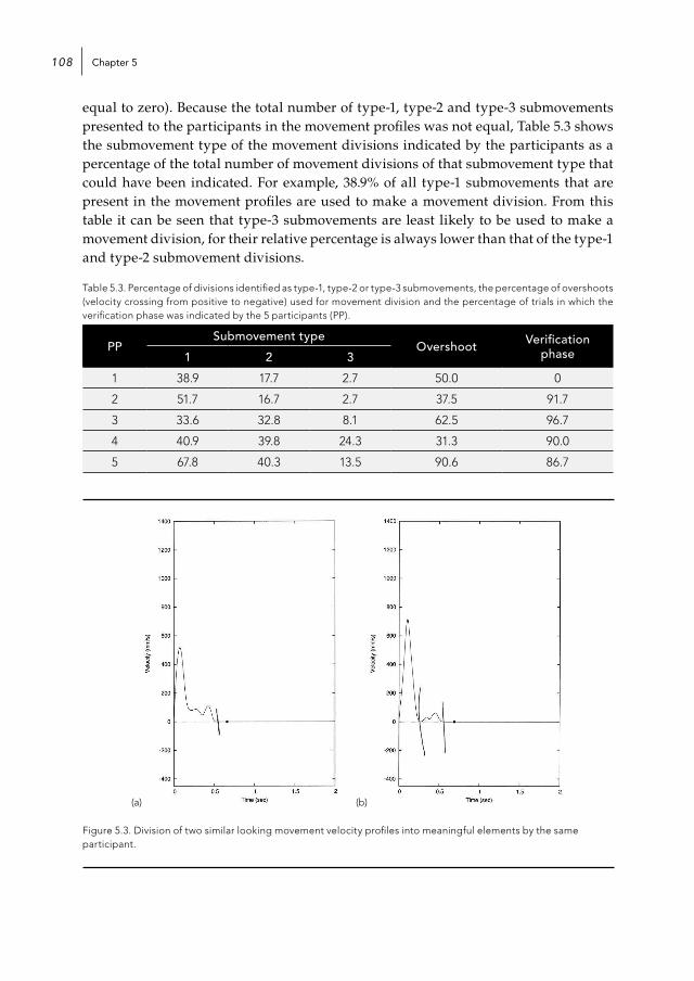
Chapter 5108
equal to zero). Because the total number of type-1, type-2 and type-3 submovements presented to the participants in the movement profiles was not equal, Table 5.3 shows the submovement type of the movement divisions indicated by the participants as a percentage of the total number of movement divisions of that submovement type that could have been indicated. For example, 38.9% of all type-1 submovements that are present in the movement profiles are used to make a movement division. From this table it can be seen that type-3 submovements are least likely to be used to make a movement division, for their relative percentage is always lower than that of the type-1 and type-2 submovement divisions.
Table 5.3. Percentage of divisions identified as type-1, type-2 or type-3 submovements, the percentage of overshoots (velocity crossing from positive to negative) used for movement division and the percentage of trials in which the verification phase was indicated by the 5 participants (PP).
PPSubmovement type
Overshoot Verification phase1 2 3
1 38.9 17.7 2.7 50.0 0
2 51.7 16.7 2.7 37.5 91.7
3 33.6 32.8 8.1 62.5 96.7
4 40.9 39.8 24.3 31.3 90.0
5 67.8 40.3 13.5 90.6 86.7
(a) (b)
Figure 5.3. Division of two similar looking movement velocity profiles into meaningful elements by the same participant.

Movement phases 109
Type-1 submovements are most likely to be used to make a movement division and especially events when the cursor stops moving (pauses) are strong indicators for the end of a movement phase. Figure 5.3 shows an example of the previously described observation. This figure shows two different velocity profiles, which are processed by the same participant. The velocity profiles are quite similar to each other, but an essential difference is that in the first movement profile (Figure 5.3a) the cursor doesn’t come to a hold before the target is reached, whereas in the second movement profile (Figure 5.3b) the cursor shortly stops before the target is reached. As can be seen in the first case both type-2 submovements are not used to indicate a movement division, whereas in the second case only the type-1 submovement is used to indicate the end of a movement phase.
Another important observation is that an overshoot with a velocity zero-crossing from positive to negative, which is one of the three criteria Meyer et al. (1988) proposed to divide movements into submovements, is not always used to indicate the end of a movement phase. Table 5.3 shows the percentage of overshoots participants use to indicate the end of a movement phase. Only one participant systematically uses the overshoot to indicate the end of a movement phase and the other participants only use it about half of the time. From the movement profiles it can be seen that especially when the path fluently continues after passing by the target, the velocity zero-crossing is not used to indicate the end of a movement phase. This is illustrated in Figure 5.4, which shows the division of the same overshoot movement (Figure 5.4a) into phases by two participants. In both cases the division is indicated at the first pause after the pointer returned to the target and not at the velocity zero-crossing (see Figure 5.4b and Figure 5.4c).
(a) (b) (c)
Figure 5.4. Goal-directed movement overshooting the target: a) traveled path, b & c) corresponding velocity profile with a division into meaningful elements by two participants.

Chapter 5110
As can also be seen in Table 5.3 four participants consistently indicate a border at the position where the cursor stopped moving, just before the target selection. This indicates that also parts in which no movement occurs can be characterized as meaningful. Movement characteristics that are further noticed are the small submovements before the large movement towards the target is initiated. Only one of the movement profiles presented to the participants contained a substantial submovement before the larger ballistic movement. Three of the five participants discern this submovement from the rest of the movement. Three other movement profiles contained a small submovement before the large movement towards the target. One participant consistently discerns these small submovements from the rest of the movements. This indicates that not only the small submovements at the end but also the small submovements at the beginning of the interaction movements are valuable to discriminate.
5.2.3 Summary and considerationsAlthough no stringent conclusions can be drawn from the explorative study the findings confirm that a division in a ballistic phase and a correction phase (as proposed by Woodworth, 1899) is an intuitive division. However, also the phase at the end of the movement in which the cursor does not move anymore (i.e. verification phase) is considered important. This supports the identification of additional phases at the beginning and the end of the movement in which no movement occurs as proposed by Thompson, McConnell, Slocum, and Bohan (2007). Although none of the movements presented to the participants contained a latency phase (time before the cursor started moving), it is considered of similar value as the verification phase. Furthermore, not only the small (sub)movements at the end of the interaction movement (i.e. correction phase) but also the small (sub)movements at the beginning are valuable to discriminate. This means that several different phases of movement should be identified with a parsing method:
- Latency phase: phase before the actual movement is initiated, i.e. this phase can be seen as the preparation phase
- Initiation phase: phase in which small (sub)movements are made before the ballistic movement, often perpendicular or opposite to the task axis. This phase can be seen as a coordination/orientation phase. Although in the case of mouse and trackball interactions the occurrence of small (sub)movements before the ballistic movement is relatively low, they are possibly more common when using other input devices or interaction techniques.
- Ballistic phase: phase in which the target is approached and the largest distance is crossed. This phase is characterized by a high peak speed.
- Correction phase: phase in which the movement is continued by correcting the error made during the ballistic phase. Several additional (sub)movements are sometimes necessary to reach the target and these movements are characterized by relatively low peak speeds. In addition, in most of the cases a shorter distance is traveled than in the ballistic phase.
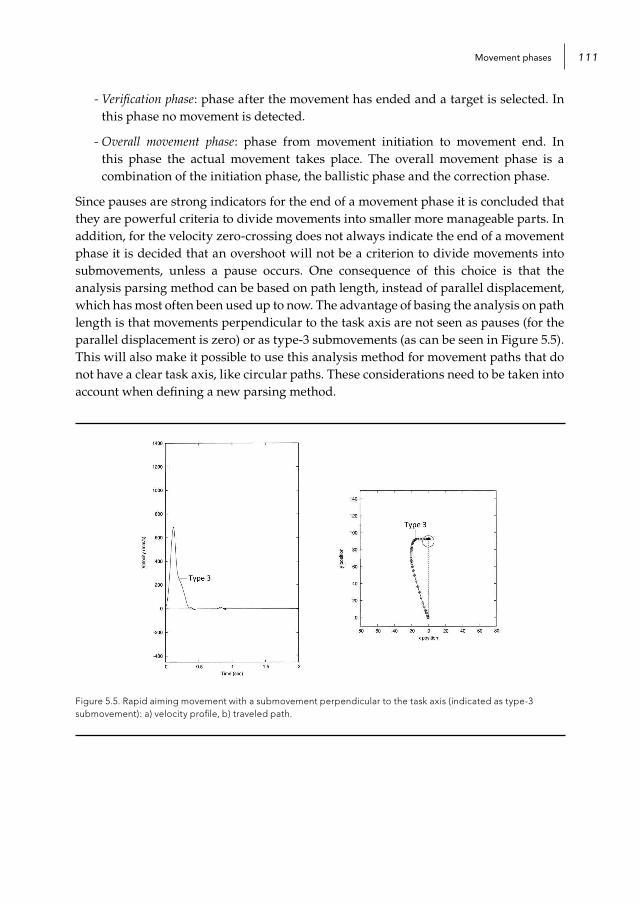
Movement phases 111
- Verification phase: phase after the movement has ended and a target is selected. In this phase no movement is detected.
- Overall movement phase: phase from movement initiation to movement end. In this phase the actual movement takes place. The overall movement phase is a combination of the initiation phase, the ballistic phase and the correction phase.
Since pauses are strong indicators for the end of a movement phase it is concluded that they are powerful criteria to divide movements into smaller more manageable parts. In addition, for the velocity zero-crossing does not always indicate the end of a movement phase it is decided that an overshoot will not be a criterion to divide movements into submovements, unless a pause occurs. One consequence of this choice is that the analysis parsing method can be based on path length, instead of parallel displacement, which has most often been used up to now. The advantage of basing the analysis on path length is that movements perpendicular to the task axis are not seen as pauses (for the parallel displacement is zero) or as type-3 submovements (as can be seen in Figure 5.5). This will also make it possible to use this analysis method for movement paths that do not have a clear task axis, like circular paths. These considerations need to be taken into account when defining a new parsing method.
Figure 5.5. Rapid aiming movement with a submovement perpendicular to the task axis (indicated as type-3 submovement): a) velocity profile, b) traveled path.
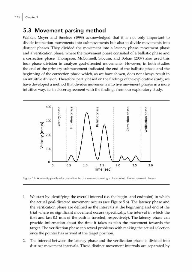
Chapter 5112
5.3 Movement parsing methodWalker, Meyer and Smelcer (1993) acknowledged that it is not only important to divide interaction movements into submovements but also to divide movements into distinct phases. They divided the movement into a latency phase, movement phase and a verification phase, where the movement phase consisted of a ballistic phase and a correction phase. Thompson, McConnell, Slocum, and Bohan (2007) also used this four phase division to analyze goal-directed movements. However, in both studies the end of the primary submovement indicated the end of the ballistic phase and the beginning of the correction phase which, as we have shown, does not always result in an intuitive division. Therefore, partly based on the findings of the explorative study, we have developed a method that divides movements into five movement phases in a more intuitive way, i.e. in closer agreement with the findings from our exploratory study.
Figure 5.6. A velocity profile of a goal-directed movement showing a division into five movement phases.
1. We start by identifying the overall interval (i.e. the begin- and endpoint) in which the actual goal-directed movement occurs (see Figure 5.6). The latency phase and the verification phase are defined as the intervals at the beginning and end of the trial where no significant movement occurs (specifically, the interval in which the first and last 0.1 mm of the path is traveled, respectively). The latency phase can provide information about the time it takes to plan the movement towards the target. The verification phase can reveal problems with making the actual selection once the pointer has arrived at the target position.
2. The interval between the latency phase and the verification phase is divided into distinct movement intervals. These distinct movement intervals are separated by

Movement phases 113
pauses in which no or only minimal movement of the pointer occurs. A pause is defined as an interval in which the speed of the pointer remains below 0.02 times the movement’s peak speed. In contrast to earlier studies we propose to determine the speed of the pointer along the movement path instead of considering the parallel displacement of the pointer. Path length is used to determine the pointer’s speed because the displacement velocity profile cannot discern real pauses from intervals in which the pointer moves perpendicular to the task axis. In addition, the analysis based on path length does not require a known task axis like the analysis based on parallel displacement, which makes it easier to extend the method to other tasks (such as circular steering tasks).
3. For each identified movement interval it is determined whether or not it makes a considerable contribution to approaching the target. If the path length of a movement interval is contributing more than 25% to the total path length it is considered to be part of the ballistic phase. This criterion is introduced to be able to deal with cases where several movements are required to reach the target, such as the one depicted in Figure 5.a. If a movement interval does not make a considerable contribution it can be part of the initiation phase, the correction phase or the ballistic phase. The movement interval will be considered part of the initiation phase when it occurs before the first ballistic movement and it will be considered part of the correction phase when it occurs after the last ballistic movement. Otherwise it will be considered part of the ballistic phase (in between large movement intervals).
4. Finally, the separate movement intervals are divided into submovements. We do this for two reasons. First, we use this division to get more detailed information on how the movement was performed (i.e., fluently or with corrections). Second, we use this division to determine whether or not the last movement interval of the ballistic phase contains some correction submovements at the end. The criteria proposed by Meyer et al. (1988) were adjusted so they could be applied to speed profiles based on path length:
a. type-1 submovement starts when the speed becomes (almost) zero (less than 0.02 times the movement’s peak speed), which means that a submovement can only occur at the beginning of a movement interval;
b. type-2 submovement starts at a zero-crossing of acceleration from negative to positive (in combination with a positive jerk that exceeds 0.01 times the maximally observed jerk3) and hence corresponds to a local minimum in the velocity profile;
c. type-3 submovement starts at a zero-crossing of jerk from positive to negative (in combination with a negative value of its derivative that exceeds 0.01 times the maximally observed value).
3 Jerk is the derivative of acceleration
Chapter 5114
The thresholds on the slopes of the zero-crossings are incorporated to avoid sub movement detection during small involuntary tremor or slow drift. The minimal requirements for submovements proposed by Meyer et al. (1988) are specific for their 1D rotation task, and need to be adapted for the case of a 2D movement path. The following minimal requirements for a submovement (to avoid the division of movements into meaningless small submovements) are: a submovement should traverse a distance of at least 1 mm and last for at least 50 ms, while the maximum velocity should exceed 0.02 times the maximally observed velocity. Submovements that do not meet this requirement are combined with bordering submovements.
If the last movement in the ballistic phase consists of multiple submovements the ballistic phase ends at the first type-2 submovement that occurs in the last 75%-95% of the traveled path length. The corrective submovements that occur during the final part of the interaction movement are considered to assist in positioning the pointer within the target boundaries. They should hence be considered as being part of the correction phase. As mentioned before, type-3 submovements are only considered to be indications of subtle accuracy regulation and are therefore not used to signal the end of the ballistic phase. If the last ballistic movement consists of only one submovement the end of this movement coincides with the end of the ballistic phase.
In order to draw meaningful conclusions from interaction movements we believe it is not only important to divide interaction movements into meaningful components, but also to assess the key characteristics of these movement phases. Especially the characterization of the ballistic phase and the correction phase by means of the position- and velocity-based measures might be of additional value when describing movement quality.
5.4 Experiment
5.4.1 Research questionAs in the previous chapter, we will start by investigating the patterns revealed by the simplest form of characterizing movement quality, namely the duration and occurrence of the identified movement phases. Subsequently, we will also focus on the identification and interpretation of patterns (of main and interaction effects) revealed by the position-based and velocity-based measures applied to the ballistic and the correction phase. Based on the division of movements into phases and the characterization of these phases we would like to answer the following questions:
Are the occurrence and the duration of the various movement phases able to reveal different patterns in the data (i.e. main and interaction effects) compared to the overall movement duration in the case of the selection task and the tracing task?
Movement phases 115
What patterns (main and interaction effects) do phase-based measures reveal and are they different from the aspects already captured by the phase duration and phase occurrence measures in the case of the selection task and the tracing task?
- Do ballistic phase measures reveal patterns that are different or similar from the patterns revealed by the correction phase measures?
- Do phase-based measures reveal patterns that are different or similar from the patterns revealed by the overall movement measures?
What phase-based measures can best describe the differences between input devices (mouse and stylus) with respect to movement quality in the case of the selection task and the tracing task?
5.4.2 Method
5.4.2.1 Experimental set-upThe data from the 2D experiment described in Chapter 2 will also be used to investigate the additional value of the measures characterizing the different movement phases. For the full description of the experimental set-up see Section 2.3.1.
5.4.2.2 Input data filtering The position data was filtered as a function of time since taking derivatives of noisy signals easily gives rise to spurious details. The data was filtered using a Gaussian time filter with a standard deviation of 25 ms, which is comparable to the 7 Hz low-pass filter proposed in earlier studies. The advantage of a Gaussian filter is that it is known not to introduce spurious details, as explained in the theory of scale space filtering (Koenderink, 1984).
5.4.3 Results movement phases
5.4.3.1 Phase occurrenceUnivariate analysis of variance is applied to the phase occurrence measure with participant as random factor4 to identify significant main and interaction effects (or ‘patterns’). The model further includes input device (mouse and stylus), orientation (horizontal-vertical and oblique), distance (3 difficulty levels) and target size or tunnel width (3 difficulty levels) as independent variables. The selection task data and tracing task data are analyzed separately. Since all of the trials contain a ballistic phase, the occurrence measure does not contain any discriminative information with respect to the ballistic phase and is not taken into account in the parametric analysis.
4 Treating participant as a random factor is equivalent to a repeated-measures analysis.

Chapter 5116
(a) (b)
Figure 5.7. Phase occurrence (with 95% confidence intervals) as a function of the input device (mouse/stylus) for: a) the selection task, b) the tracing task.
Figure 5.7 shows the average frequency of the different movement phases while using the mouse and the stylus during the selection task (see Figure 5.7a) and the tracing task (see Figure 5.7b). With respect to the selection task (see Figure 5.7a), it can be seen that the occurrence of the latency phase and the initiation phase is higher when using the stylus than when using the mouse. On the other hand, the correction phase and the verification phase occur more often when using the mouse than when using the stylus. These results show that the movement initiation proceeds smoother when using the mouse (i.e. lower frequency of the latency and initiation phase), however, the approach towards the target is less efficient. As a result, more corrections are required to end up at the target area. Furthermore, the higher frequency of the verification phase might indicate that the movement termination is somewhat easier when using the stylus than when using the mouse.
Table 5.4 presents the ANOVA results applied to the frequency occurrence (after log-odds ratio transformation5) in terms of the F-value and the effect size (partial eta-squared). According to Cohen (1992) a partial eta-squared of .50-.80 is considered a medium effect and anything equal to or greater than .80 can be considered a large effect size. The ANOVA results confirm that the main effects of input device are significant for these four movement phases. In addition, the latency phase occurrence shows a significant interaction effect between input device and target distance, whereas the verification phase occurrence shows a significant interaction effect between input device and target size (see Table 5.4). As the distance becomes larger, the difference between the mouse and the stylus with respect to the latency occurrence also increases. With respect to the verification phase the difference between the mouse and the stylus decreases as the target becomes smaller.
5 The log-odds ratio is an often used transformation applied to frequency data in order to approximate the standard normal distribution (Azen & Walker, 2010).
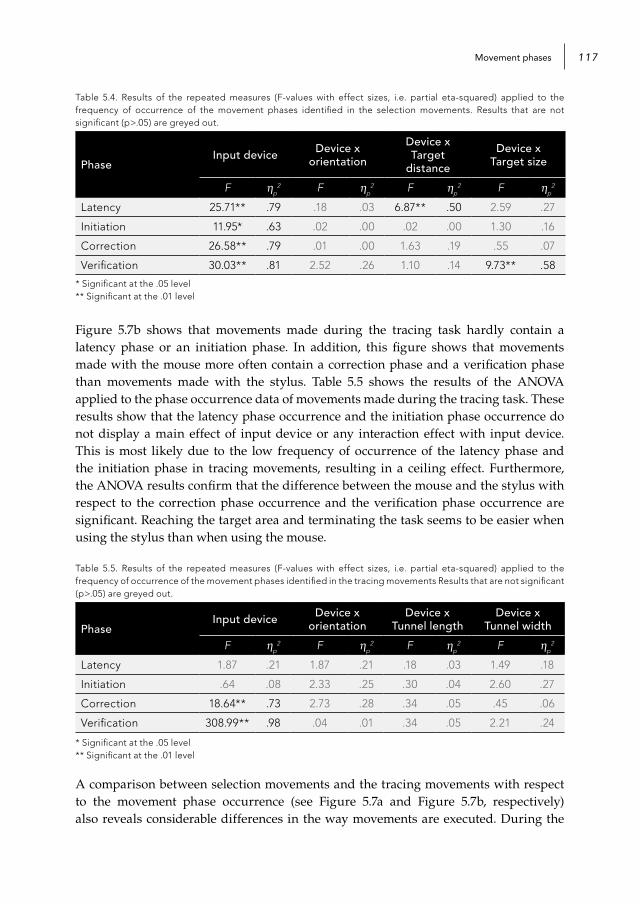
Movement phases 117
Table 5.4. Results of the repeated measures (F-values with effect sizes, i.e. partial eta-squared) applied to the frequency of occurrence of the movement phases identified in the selection movements. Results that are not significant (p>.05) are greyed out.
PhaseInput device Device x
orientation
Device xTarget
distance
Device xTarget size
F ηp2 F ηp
2 F ηp2 F ηp
2
Latency 25.71** .79 .18 .03 6.87** .50 2.59 .27
Initiation 11.95* .63 .02 .00 .02 .00 1.30 .16
Correction 26.58** .79 .01 .00 1.63 .19 .55 .07
Verification 30.03** .81 2.52 .26 1.10 .14 9.73** .58
* Significant at the .05 level** Significant at the .01 level
Figure 5.7b shows that movements made during the tracing task hardly contain a latency phase or an initiation phase. In addition, this figure shows that movements made with the mouse more often contain a correction phase and a verification phase than movements made with the stylus. Table 5.5 shows the results of the ANOVA applied to the phase occurrence data of movements made during the tracing task. These results show that the latency phase occurrence and the initiation phase occurrence do not display a main effect of input device or any interaction effect with input device. This is most likely due to the low frequency of occurrence of the latency phase and the initiation phase in tracing movements, resulting in a ceiling effect. Furthermore, the ANOVA results confirm that the difference between the mouse and the stylus with respect to the correction phase occurrence and the verification phase occurrence are significant. Reaching the target area and terminating the task seems to be easier when using the stylus than when using the mouse.
Table 5.5. Results of the repeated measures (F-values with effect sizes, i.e. partial eta-squared) applied to the frequency of occurrence of the movement phases identified in the tracing movements Results that are not significant (p>.05) are greyed out.
PhaseInput device Device x
orientationDevice x
Tunnel lengthDevice x
Tunnel width
F ηp2 F ηp
2 F ηp2 F ηp
2
Latency 1.87 .21 1.87 .21 .18 .03 1.49 .18
Initiation .64 .08 2.33 .25 .30 .04 2.60 .27
Correction 18.64** .73 2.73 .28 .34 .05 .45 .06
Verification 308.99** .98 .04 .01 .34 .05 2.21 .24
* Significant at the .05 level** Significant at the .01 level
A comparison between selection movements and the tracing movements with respect to the movement phase occurrence (see Figure 5.7a and Figure 5.7b, respectively) also reveals considerable differences in the way movements are executed. During the
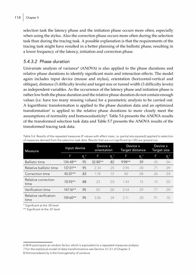
Chapter 5118
selection task the latency phase and the initiation phase occurs more often, especially when using the stylus. Also the correction phase occurs more often during the selection task than during the tracing task. A possible explanation is that the requirements of the tracing task might have resulted in a better planning of the ballistic phase, resulting in a lower frequency of the latency, initiation and correction phase.
5.4.3.2 Phase durationUnivariate analysis of variance6 (ANOVA) is also applied to the phase durations and relative phase durations to identify significant main and interaction effects. The model again includes input device (mouse and stylus), orientation (horizontal-vertical and oblique), distance (3 difficulty levels) and target size or tunnel width (3 difficulty levels) as independent variables. As the occurrence of the latency phase and initiation phase is rather low both the phase duration and the relative phase duration do not contain enough values (i.e. have too many missing values) for a parametric analysis to be carried out. A logarithmic transformation is applied to the phase duration data and an optimized transformation7 is applied to the relative phase durations to more closely meet the assumptions of normality and homoscedasticity8. Table 5.6 presents the ANOVA results of the transformed selection task data and Table 5.7 presents the ANOVA results of the transformed tracing task data.
Table 5.6. Results of the repeated measures (F-values with effect sizes, i.e. partial eta-squared) applied to selection of measures derived from the selection task data. Results that are not significant (p>.05) are greyed out.
MeasureInput device Device x
orientationDevice x
Target distanceDevice x
Target size
F ηp2 F ηp
2 F ηp2 F ηp
2
Ballistic time 134.48** .95 32.80** .82 9.98** .59 .45 .06
Relative ballistic time 137.01** .95 2.34 .25 2.94 .30 .71 .09
Correction time 45.07** .83 1.18 .13 .82 .08 .26 .03
Relative correction time 70.93** .88 .23 .03 1.43 .13 .13 .02
Verification time 147.16** .95 .05 .00 3.54 .29 .77 .09
Relative verification time 159.60** .95 3.06 .24 2.11 .20 .91 .10
* Significant at the .05 level** Significant at the .01 level
6 With participant as random factor, which is equivalent to a repeated-measures analysis.7 For the statistical model of data transformations see Section 3.1.3.1 of Chapter 3.8 Homoscedasticity is the homogeneity of variance.

Movement phases 119
Table 5.7. Results of the repeated measures (F-values with effect sizes, i.e. partial eta-squared) applied to selection of measures derived from the tracing task data. Results that are not significant (p>.05) are greyed out.
MeasureInput device Device x
orientationDevice x
Tunnel lengthDevice x
Tunnel width
F ηp2 F ηp
2 F ηp2 F ηp
2
Ballistic time 1.34 .16 45.83** .87 32.59** .82 88.15** .93
Relative ballistic time 124.49** .95 10.28* .60 5.34* .43 34.28** .83
Correction time 97.66** .93 .09 .02 9.63** .59 3.69 .36
Relative correction time 298.06** .97 3.68 .37 5.22* .44 .12 .02
Verification time 33.78** .83 1.34 .15 2.34 .24 .24 .03
Relative verification time 27.03** .79 21.00** .72 .59 .07 7.40** .48
* Significant at the .05 level** Significant at the .01 level
The analysis of the transformed overall movement time presented in the previous chapter (see Section 4.3.3.1) did not reveal any differences between the mouse and the stylus. However, the results in Table 5.6 and Table 5.7 clearly show a difference between the two input devices with respect to the duration of the various phases. Only the duration of the ballistic phase of tracing movements does not show a significant effect of input device. The results in these tables further show that the relative phase duration displays an equal or higher effect size than the phase duration in almost all cases. The relative duration corrects to some extent for the task difficulty since there is a close correspondence between the overall duration and the task difficulty. Therefore, we prefer to use the relative duration, complementary to the overall movement duration, to describe the differences between the two input devices.
Figure 5.8 shows the relative duration of the ballistic, correction and verification phase when using the mouse and the stylus during the selection task (see Figure 5.8a) and the tracing task (see Figure 5.8b). Figure 5.8a shows that the proportion of the ballistic phase (of the total selection time) is larger when using the stylus than when using the mouse. On the other hand the relative duration of the correction and the verification phase are longer when using the mouse than when using the stylus. The same pattern can be observed for the tracing task data. Furthermore, the significant interaction effects show that the task difficulty of the tracing task has a large impact on the difference in performance of the two input devices. The more difficult the task the worse the performance of the mouse compared to the stylus.
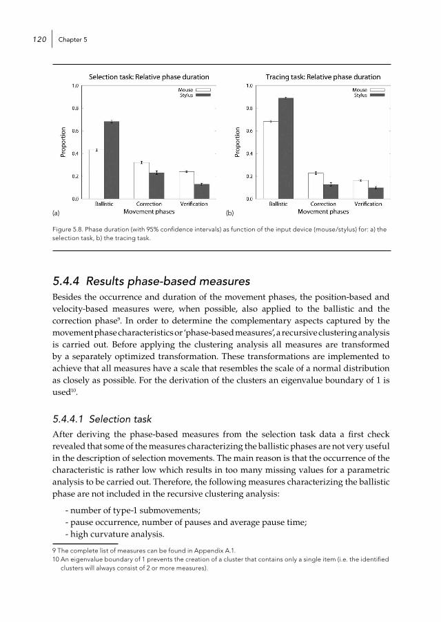
Chapter 5120
(a) (b)
Figure 5.8. Phase duration (with 95% confidence intervals) as function of the input device (mouse/stylus) for: a) the selection task, b) the tracing task.
5.4.4 Results phase-based measuresBesides the occurrence and duration of the movement phases, the position-based and velocity-based measures were, when possible, also applied to the ballistic and the correction phase9. In order to determine the complementary aspects captured by the movement phase characteristics or ‘phase-based measures’, a recursive clustering analysis is carried out. Before applying the clustering analysis all measures are transformed by a separately optimized transformation. These transformations are implemented to achieve that all measures have a scale that resembles the scale of a normal distribution as closely as possible. For the derivation of the clusters an eigenvalue boundary of 1 is used10.
5.4.4.1 Selection taskAfter deriving the phase-based measures from the selection task data a first check revealed that some of the measures characterizing the ballistic phases are not very useful in the description of selection movements. The main reason is that the occurrence of the characteristic is rather low which results in too many missing values for a parametric analysis to be carried out. Therefore, the following measures characterizing the ballistic phase are not included in the recursive clustering analysis:
- number of type-1 submovements; - pause occurrence, number of pauses and average pause time; - high curvature analysis.
9 The complete list of measures can be found in Appendix A.1. 10 An eigenvalue boundary of 1 prevents the creation of a cluster that contains only a single item (i.e. the identified
clusters will always consist of 2 or more measures).

Movement phases 121
In the case of the description of the correction phase the average pause time was not included in the recursive clustering analysis due to the low occurrence rate.
Table 5.8. Clustering of measures according to the patterns identified with the 1D recursive clustering analysis of the phase-based measures applied to the ballistic phase of the selection movements.
Cluster B1(Cronbach’s Alpha = .98)
Cluster B2(Cronbach’s Alpha = .99)
Measure R P Measure R P
Number of submovements .99 .04 Movement error 1.0 .01
Acceleration time .99 .05 Movement variability .99 .04
Number of type-3 submovements .99 .05 Movement offset .99 .04
Time to peak speed .99 .06
Ballistic phase duration .98 .06
Deceleration time .96 .08
Number of type-2 submovements .90 .13
Relative duration of ballistic phase .90 .15
Relative time to peak speed .75 .17
Cluster B3(Cronbach’s Alpha = .86)
Cluster B4(Cronbach’s Alpha = .95)
Measure R P Measure R P
Task axis crossing .92 .09 Peak speed 1.0 .02
Movement direction change .90 .11 Average speed .99 .05
Orthogonal direction change .80 .21 Peak acceleration .93 .12
Path length efficiency .74 .18 Peak deceleration .92 .13
Path length .71 .26
The recursive clustering analysis reveals four clusters within the phase-based measures derived from the ballistic phase of the selection movements. Table 5.8 shows the four clusters together with the Cronbach’s Alpha, the correlations of the measures with the corresponding pattern (R-values) and the corresponding P-values11. The internal consistency of the four clusters is high, shown by the large Cronbach’s alpha values (>.86). All measures show a relatively good fit with the cluster they are appointed to (R>.71).
11 P-value is the ratio between the error and the variation in the data. Lower P-values indicate a measure with more discriminative power (higher signal-to-noise ratio).
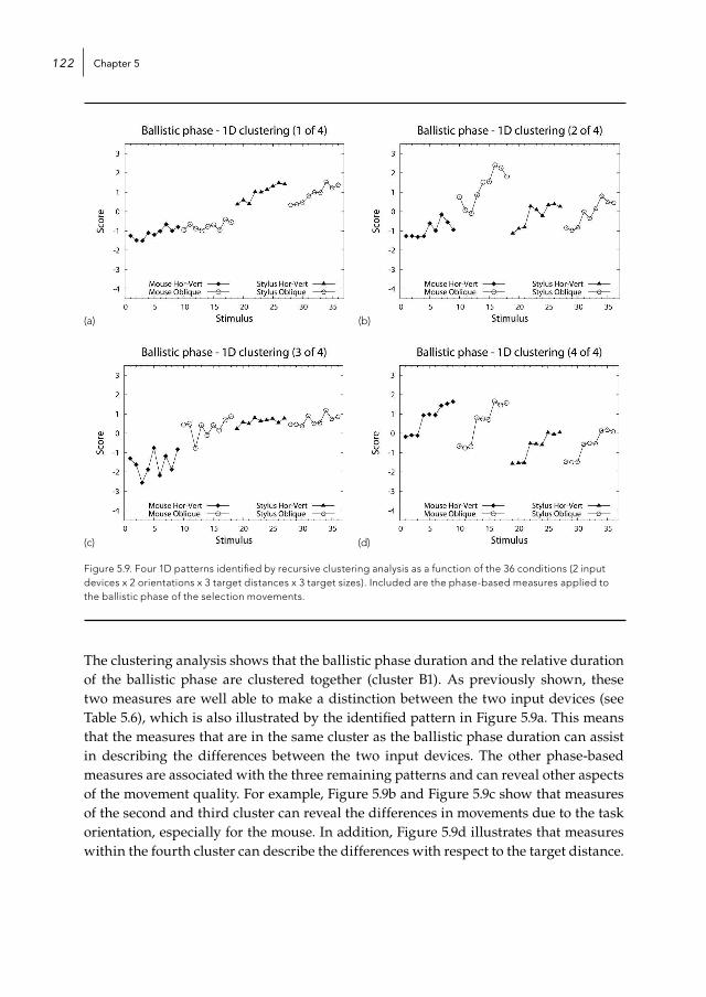
Chapter 5122
(a) (b)
(c) (d)
Figure 5.9. Four 1D patterns identified by recursive clustering analysis as a function of the 36 conditions (2 input devices x 2 orientations x 3 target distances x 3 target sizes). Included are the phase-based measures applied to the ballistic phase of the selection movements.
The clustering analysis shows that the ballistic phase duration and the relative duration of the ballistic phase are clustered together (cluster B1). As previously shown, these two measures are well able to make a distinction between the two input devices (see Table 5.6), which is also illustrated by the identified pattern in Figure 5.9a. This means that the measures that are in the same cluster as the ballistic phase duration can assist in describing the differences between the two input devices. The other phase-based measures are associated with the three remaining patterns and can reveal other aspects of the movement quality. For example, Figure 5.9b and Figure 5.9c show that measures of the second and third cluster can reveal the differences in movements due to the task orientation, especially for the mouse. In addition, Figure 5.9d illustrates that measures within the fourth cluster can describe the differences with respect to the target distance.

Movement phases 123
To support the observations based on the patterns in Figure 5.9, ANOVA analyses are applied to the standardized values of the identified patterns. Due to the lack of degrees of freedom, only the main effects of the independent variables (input device, orientation, target distance and target size) and the interaction effect between input device and orientation are included in the ANOVA model. The results are presented in Table 5.9 and confirm the observations made in the previous paragraph. The results further show that none of the patterns can make a distinction between the different target sizes (see Table 5.9). This is an indication that the execution of the ballistic phase in selection movements is rather independent of the target size.
Table 5.9. Results of the ANOVA (F-values and effect sizes, i.e. partial eta-squared) applied to the identified patterns in the phase-based measures derived from the ballistic phase of the selection movements. To emphasize the larger effects, results with an effect size <.30 are greyed out.
PatternInput device Orientation Device x
orientationTarget
distance Target size
F ηp2 F ηp
2 F ηp2 F ηp
2 F ηp2
1 773.76** .97 4.26* .13 9.90** .26 34.02** .71 .42 .03
2 8.14** .23 106.44** .79 93.46** .77 52.04** .79 .59 .04
3 98.29** .78 55.20** .66 48.76** .64 4.05* .23 .80 .05
4 752.14** .96 3.35 .11 10.28** .27 456.58** .97 .98 .00
* Significant at the .05 level** Significant at the .01 level
Table 5.10 shows the clustering of measures based on the recursive clustering analysis of the position-based measures derived from the correction phase of the selection movements. In addition, the Cronbach’s Alpha, the correlations of the measures with the corresponding pattern (R-values) and the corresponding P-values are indicated. The Cronsbach’s Alpha is larger than .90 for all three clusters, indicating that the measures in each cluster have a high internal consistency and can reveal a similar pattern in the data. The measures path length efficiency and number of type-3 submovements have a relatively low correlation with the corresponding pattern (R=.59 and R=.51). This means that these measures do not really fit within the clusters they are appointed to and that they do not correspond to any of the identified patterns. In the case of the path length efficiency this is most likely due to the lower discriminative ability of the measure itself (indicated by the relatively high P-value of .24). The P-value of the number of type-3 submovements is not very high (P=.14) which may indicate that it will better fit within an additional cluster, representing a different pattern. However, when there is only one measure representing a different pattern, the recursive clustering algorithm (with eigenvalue boundary of 1) does not see a need to create an additional cluster.

Chapter 5124
Table 5.10. Clustering of measures according to the patterns identified with the 1D recursive clustering analysis of the phase-based measures applied to the correction phase of the selection movements.
Cluster C1(Cronbach’s Alpha = .95)
Cluster C2(Cronbach’s Alpha = .90)
Measure R P Measure R P
Peak speed .96 .08 Acceleration time .88 .13
Path length .94 .10 Number of pauses .85 .09
Peak deceleration .94 .11 Pause occurrence .85 .09
Peak acceleration .88 .13 Time to peak speed .81 .13
Movement error .87 .11 Number of type-1 submovements .79 .14
Average speed .87 .14 Movement direction change .64 .17
Movement variability .85 .12 Orthogonal direction change .64 .18
Movement offset .81 .13 High curvature analysis .63 .19
Task axis crossing .70 .20
Path length efficiency .59 .24
Cluster C3(Cronbach’s Alpha = .93)
Measure R P
Deceleration time .95 .07
Correction phase duration .95 .08
Relative duration of correction phase .90 .12
Number of submovements .88 .10
Relative time to peak speed .85 .13
Number of type-2 submovements .73 .16
Correction phase occurrence .71 .14
Number of type-3 submovements .51 .14
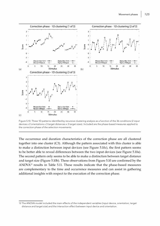
Movement phases 125
(a) (b)
(c)
Figure 5.10. Three 1D patterns identified by recursive clustering analysis as a function of the 36 conditions (2 input devices x 2 orientations x 3 target distances x 3 target sizes). Included are the phase-based measures applied to the correction phase of the selection movements.
The occurrence and duration characteristics of the correction phase are all clustered together into one cluster (C3). Although the pattern associated with this cluster is able to make a distinction between input devices (see Figure 5.10c), the first pattern seems to be better able to reveal differences between the two input devices (see Figure 5.10a). The second pattern only seems to be able to make a distinction between target distance and target size (Figure 5.10b). These observations from Figure 5.10 are confirmed by the ANOVA12 results in Table 5.11. These results indicate that the phase-based measures are complementary to the time and occurrence measures and can assist in gathering additional insights with respect to the execution of the correction phase.
12 The ANOVA model included the main effects of the independent variables (input device, orientation, target distance and target size) and the interaction effect between input device and orientation.

Chapter 5126
Table 5.11. Results of the ANOVA (F-values and effect sizes, i.e. partial eta-squared) applied to the identified patterns in the phase-based measures derived from the correction phase of the selection movements. To emphasize the larger effects, results with an effect size <.30 are greyed out.
PatternInput device Orientation Device x
orientation Target distance Target size
F ηp2 F ηp
2 F ηp2 F ηp
2 F ηp2
1 217.18** .89 12.58** .31 21.77** .44 50.23** .78 2.00 .13
2 6.01* .18 2.27 .08 .42 .02 14.15** .50 31.59** .69
3 79.43** .74 .11 .00 9.37** .25 11.14** .44 17.69** .56
* Significant at the .05 level** Significant at the .01 level
(a) (b)
Figure 5.11. MDS results of the 1D patterns identified in a) the position-based measures derived from the ballistic phase (B1, B2, B3 and B4) and the correction phase (C1, C2 and C3) of the selection movements; b) the position-based measures derived from the ballistic phase (B1, B2, B3 and B4) and the correction phase (C1, C2 and C3) and the begin- and endpoint measures, position-based measures and the velocity-based measures derived from the selection movements (A1, A2, A3, A4 and A5, see also Figure 4.8 in Chapter 4).
Multidimensional scaling (MDS) with the proximity scaling (PROXSCAL) technique (Commandeur & Heiser, 1993) was applied to the seven identified patterns to examine the degree to which the patterns identified in the ballistic phase measures correspond to the patterns identified in the correction phase measures. Figure 5.11a shows the common space of the four patterns derived from the ballistic phase measures (B1, B2, B3 and B4) and the three patterns derived from the correction phase measures (C1, C2 and C3). It can be seen that only one ballistic phase pattern (B4) is similar to a correction phase pattern (C1). The distance between the other ballistic phase patterns and the correction phase patterns is much larger, signifying that these patterns are not quite similar. This
Movement phases 127
shows that the characterizations of both phases are complementary to each other with respect to the description of movement quality.
Not only the similarities between the ballistic phase patterns and the correction phase patterns was examined but also the similarities between these patterns and the patterns derived from the overall movement described in Chapter 4. Figure 5.11b shows the result of the MDS analysis with the proximity scaling (PROXSCAL) technique. This figure shows that all patterns identified in the measures characterizing the ballistic and correction phase can be associated with patterns identified in the measures characterizing the overall movement. This means that the characterization of the movement phases does not necessarily reveal any new trends with respect to movement quality, but rather provides a more detailed description of movement quality.
5.4.4.2 Tracing taskAlso in the case of the tracing task, several measures characterizing the ballistic and correction phases are not very useful due to the low occurrence rate. Therefore, the following measures characterizing the ballistic phase are not included in the recursive clustering analysis:
- number of type-1 submovement; - pause occurrence, number of pauses and average pause time; - high curvature analysis; - orthogonal direction phase.
In the case of the description of the correction phase the following measures are not included in the recursive clustering analysis due to the low occurrence rate:
- orthogonal direction changes; - number of pauses and average pause time.
The recursive clustering analysis, applied to the phase-based measures derived from the ballistic phase of the tracing movements, reveals four clusters. Table 5.12 shows the four clusters together with the Cronbach’s Alpha, the correlations of the measures with the corresponding pattern (R-values) and the corresponding P-values. Again, the internal consistency of the four clusters is high, shown by the large Cronbach’s alpha values (>.86) and all measures show a relatively good fit with the cluster they are appointed to (R>.75).

Chapter 5128
Table 5.12. Clustering of the measures according to the patterns identified with the 1D recursive clustering analysis of the phase-based measures applied to the ballistic phase of the tracing movements.
Cluster B1(Cronbach’s Alpha = .98)
Cluster B2(Cronbach’s Alpha = .95)
Measure R P Measure R P
Ballistic phase duration .99 .03 Peak speed .97 .06
Deceleration time .99 .04 Peak deceleration .96 .09
Acceleration time .98 .04 Peak acceleration .91 .12
Number of submovements .98 .04 Average speed .87 .11
Number of type-2 submovements .97 .05
Movement direction change .90 .09
Number of type-3 submovements .88 .11
Task axis crossing .78 .14
Path length .75 .25
Clustera B3(Cronbach’s Alpha = .92)
Cluster B4(Cronbach’s Alpha = .86)
Measure R P Measure R P
Movement error .98 .05 Relative duration of ballistic phase .95 .10
Movement variability .94 .08 Time to peak speed .92 .11
Movement offset .87 .11 Relative time to peak speed .79 .15
Path length efficiency .78 .18
The results of the clustering analysis show that the ballistic phase duration and the relative duration of the ballistic phase are not clustered together. The ANOVA results in Table 5.7 (see Section 5.4.3.2) already showed that of these two measures only the relative duration of the ballistic phase can make a distinction between the two input devices. This large effect of input device is also illustrated by the pattern in Figure 5.12d, which is associated with the cluster containing the relative duration of the ballistic phase. The pattern of the first cluster containing the ballistic phase duration measure does not only display an effect of orientation, but also a clear effect of tunnel length and tunnel width (see Figure 5.12a).
Since the duration measures of the ballistic phase are part of two separate clusters (B1 and B4), there are two clusters of measures left that can reveal different patterns in the data compared to the ones already revealed by the duration measures. Besides an effect of input device the second pattern shown in Figure 5.12b also displays an effect of tunnel width, especially when using the mouse. The third pattern mainly shows an effect of orientation and an interaction effect between input device and orientation (see Figure 5.12c). These observations are confirmed by the ANOVA13 results presented in Table 5.13.
13 The ANOVA model included the main effects of the independent variables (input device, orientation, target distance and target size) and the interaction effect between input device and orientation.
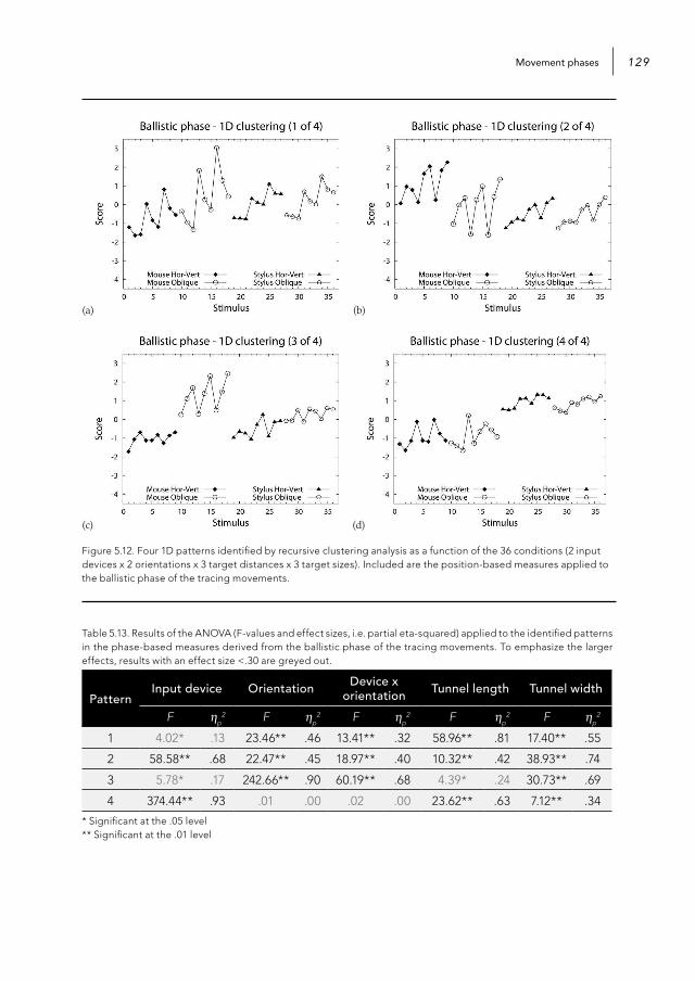
Movement phases 129
(a) (b)
(c) (d)
Figure 5.12. Four 1D patterns identified by recursive clustering analysis as a function of the 36 conditions (2 input devices x 2 orientations x 3 target distances x 3 target sizes). Included are the position-based measures applied to the ballistic phase of the tracing movements.
Table 5.13. Results of the ANOVA (F-values and effect sizes, i.e. partial eta-squared) applied to the identified patterns in the phase-based measures derived from the ballistic phase of the tracing movements. To emphasize the larger effects, results with an effect size <.30 are greyed out.
PatternInput device Orientation Device x
orientation Tunnel length Tunnel width
F ηp2 F ηp
2 F ηp2 F ηp
2 F ηp2
1 4.02* .13 23.46** .46 13.41** .32 58.96** .81 17.40** .55
2 58.58** .68 22.47** .45 18.97** .40 10.32** .42 38.93** .74
3 5.78* .17 242.66** .90 60.19** .68 4.39* .24 30.73** .69
4 374.44** .93 .01 .00 .02 .00 23.62** .63 7.12** .34
* Significant at the .05 level** Significant at the .01 level

Chapter 5130
Table 5.14. Clustering of the measures according to the patterns identified with the 1D recursive clustering analysis of the phase-based measures applied to the correction phase of the tracing movements.
Cluster C1(Cronbach’s Alpha = .97)
Cluster C2(Cronbach’s Alpha = .87)
Measure R P Measure R P
Deceleration time .99 .05 Movement error .95 .08
Correction phase duration .98 .05 Movement offset .93 .09
Path length .98 .06 Movement variability .93 .10
Relative time to peak speed .94 .11 Task axis crossing .58 .31
Path length efficiency .93 .13
Peak speed .91 .12
Number of submovements .90 .08
Peak deceleration .90 .11
Correction phase occurrence .89 .13
Number of type-2 submovements .87 .09
Acceleration time .85 .12
Number of type-3 submovements .78 .21
Time to peak speed .71 .13
Average speed .66 .21
Pause occurrence .62 .31
Movement direction change .55 .28
Cluster C3(Cronbach’s Alpha = .79)
Measure R P
Number of type-1 submovements .94 .09
Relative duration of correction phase .84 .16
High curvature analysis .67 .24
Peak acceleration .66 .17
An obvious result from the recursive clustering analysis is that the majority of the correction phase measures are clustered together in the first cluster (see Table 5.14). This is also the case for the correction phase duration and correction phase occurrence measures. Since most measures reveal the same pattern as the correction phase duration, these measures can help in understanding why the correction phase is longer when using the mouse than when using the stylus. The relative duration of the correction phase is assigned to the third cluster. This means that only measures of the second cluster can reveal an additional pattern in the data that is complementary to the ones revealed by the occurrence and duration measures of the correction phase.

Movement phases 131
(a) (b)
(c)
Figure 5.13. Three 1D patterns identified by recursive clustering analysis as a function of the 36 conditions (2 input devices x 2 orientations x 3 target distances x 3 target sizes). Included are the position-based measures applied to the correction phase of the tracing movements.
Figure 5.13 shows the three identified patterns within the phase-based measures derived from the correction phase of tracing movements as a function of the 36 conditions (2 input devices x 2 orientations x 3 target distances x 3 target sizes). This figure shows that especially the first and the third pattern are able to distinguish between the two input devices. The second pattern is better at making a distinction between the two orientations. These observations are supported by the ANOVA14 results of the patterns presented in Table 5.15. The results in this table further show that the second pattern is the only pattern that is able to make a distinction between the different tunnel widths.
14 The ANOVA model included the main effects of the independent variables (input device, orientation, target distance and target size) and the interaction effect between input device and orientation.
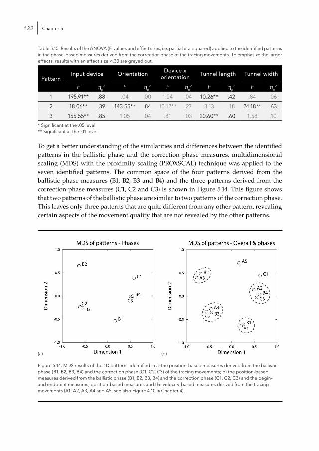
Chapter 5132
Table 5.15. Results of the ANOVA (F-values and effect sizes, i.e. partial eta-squared) applied to the identified patterns in the phase-based measures derived from the correction phase of the tracing movements. To emphasize the larger effects, results with an effect size <.30 are greyed out.
PatternInput device Orientation Device x
orientation Tunnel length Tunnel width
F ηp2 F ηp
2 F ηp2 F ηp
2 F ηp2
1 195.91** .88 .04 .00 1.04 .04 10.26** .42 .84 .06
2 18.06** .39 143.55** .84 10.12** .27 3.13 .18 24.18** .63
3 155.55** .85 1.05 .04 .81 .03 20.60** .60 1.58 .10
* Significant at the .05 level** Significant at the .01 level
To get a better understanding of the similarities and differences between the identified patterns in the ballistic phase and the correction phase measures, multidimensional scaling (MDS) with the proximity scaling (PROXSCAL) technique was applied to the seven identified patterns. The common space of the four patterns derived from the ballistic phase measures (B1, B2, B3 and B4) and the three patterns derived from the correction phase measures (C1, C2 and C3) is shown in Figure 5.14. This figure shows that two patterns of the ballistic phase are similar to two patterns of the correction phase. This leaves only three patterns that are quite different from any other pattern, revealing certain aspects of the movement quality that are not revealed by the other patterns.
(a) (b)
Figure 5.14. MDS results of the 1D patterns identified in a) the position-based measures derived from the ballistic phase (B1, B2, B3, B4) and the correction phase (C1, C2, C3) of the tracing movements; b) the position-based measures derived from the ballistic phase (B1, B2, B3, B4) and the correction phase (C1, C2, C3) and the begin- and endpoint measures, position-based measures and the velocity-based measures derived from the tracing movements (A1, A2, A3, A4 and A5, see also Figure 4.10 in Chapter 4).

Movement phases 133
Also in the case of the tracing task the similarities between the patterns of the ballistic and correction phase and the patterns derived from the overall movement described in Chapter 4 are further examined. Figure 5.14b shows the common space of the MDS analysis with the proximity scaling (PROXSCAL) technique. The results show that almost all patterns characterizing the ballistic and correction phase can be associated with patterns characterizing the overall movement. Only the distance between first pattern of the correction phase measures (C1) and a pattern characterizing the overall movement (A5) is somewhat larger. As mentioned in the previous section, this indicates that the characterization of the movement phases does not necessarily reveal new trends with respect to movement quality, but rather provides a more detailed description of movement quality.
5.4.5 Results measure selectionAlthough the phase occurrence and duration measures already provide more insight into the execution of the selection and tracing movements, the phase-based measures can provide further details of the movement execution. Another advantage of dividing movements into movement phases is that the discriminative ability of these phase-based measures might be higher than the overall movement measures. As mentioned in the previous chapter we are especially interested in the differences between the input devices. When designing and evaluating input devices this would be the main focus besides the interaction effects between the input devices and the task characteristics. For the description of the ballistic and the correction phase of the selection and tracing movements we aim at selecting five measures to describe each phase.
5.4.5.1 Selection taskThe results of the ANOVA analysis applied to the identified patterns in the measures derived from the ballistic phase of the selection movements (see Table 5.9) showed that two clusters of measures (cluster B1 and cluster B4) show the largest effect of input device. Since these two clusters together contain more than five measures we select only the measures with the highest discriminative ability (i.e. highest F-values and effect sizes). The selected measures are: a) number of type-3 submovements, b) number of submovements, c) time to peak speed, d) acceleration time and e) peak acceleration.
Univariate analysis of variance is applied to the selected measures with participant as random factor and input device (mouse and stylus), orientation (horizontal-vertical and oblique), distance (3 difficulty levels) and target size (3 difficulty levels) as independent variables. The results of the ANOVA analyses applied to the selected ballistic phase measures are presented in Table 5.16. The largest difference between the mouse and the stylus can be discerned in the number of type-3 submovements made during the ballistic phase: when using the stylus the number of type-3 submovements is larger than when using the mouse. But this also accounts for the total number of submovements. The results further show that it takes longer to reach the peak speed when using the stylus

Chapter 5134
and also the time period during which the stylus is accelerating is longer. In addition, the average speed is much lower when using the stylus than when using the mouse. These differences between the mouse and the stylus can be explained by the control-to-display ratio (1:4) of the mouse compared to that of the stylus (1:1). This enables users to move faster with the mouse and to reach the peak speed faster, resulting in a shorter acceleration period.
Table 5.16. Results of the repeated measures (F-values with effect sizes, i.e. partial eta-squared) applied to the selected phase-based measures derived from the ballistic phase of selection movements. Results that are not significant (p>.05) are greyed out.
MeasureInput device Device x
orientation
Device xtarget
distance
Device xtarget size
F ηp2 F ηp
2 F ηp2 F ηp
2
Type-3 submovements 124.97** .95 3.40 .33 9.75** .58 .06 .01
Number of submovements 107.44** .94 20.67** .75 17.30** .71 .41 .06
Time to peak speed 100.87** .94 1.15 .14 5.05* .42 .35 .05
Acceleration time 88.95** .93 15.50** .69 11.45** .62 1.42 .17
Average speed 87.12** .93 31.62** .66 7.01** .50 .72 .09
* Significant at the .05 level** Significant at the .01 level
The results in Table 5.16 also show some interaction effects between input device and orientation. This is because the targets placed in the oblique direction result in a larger number of submovements, longer acceleration time and lower peak acceleration when using the mouse, whereas for the stylus this is not the case. This is an indication that when using the mouse the selection task is more difficult when the targets are placed in the oblique direction. Also, when the distance becomes larger, the difference between the stylus and the mouse becomes larger with respect to all five measures. This indicates that the target distance has a large impact on the execution of the ballistic phase of selection movements.
The identified patterns with respect to the measures derived from the correction phase of the selection movements (see Table 5.11) showed that one cluster of measures (cluster C1) is able to make the best distinction between input devices. This cluster contains ten measures, which means that only half of these measures will be selected to describe the correction phase based on their discriminative ability (i.e. highest F-values and effect sizes). The selected measures are: a) peak speed, b) path length, c) peak deceleration, d) movement error and e) peak acceleration.
Table 5.17 presents the results of the univariate analysis of variance applied to the selected correction phase measures. The model included participant as random factor and input device (mouse and stylus), orientation (horizontal-vertical and oblique), distance (3
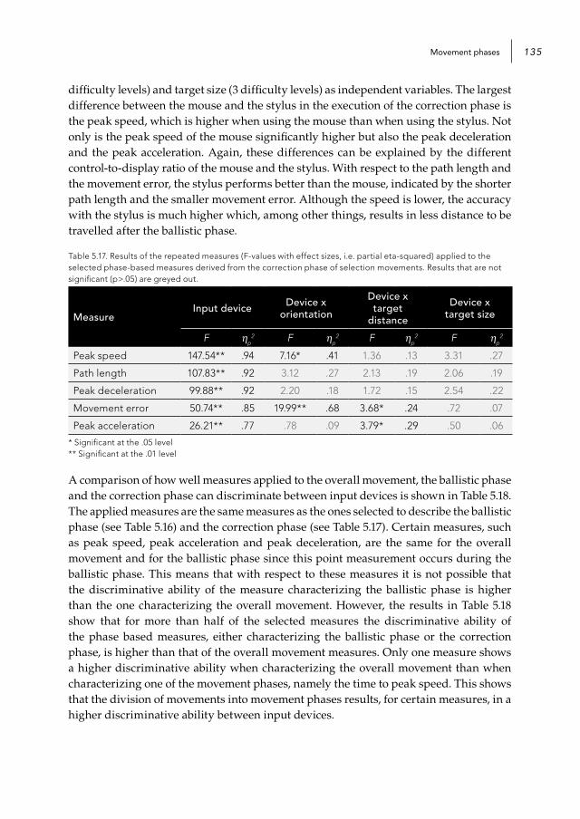
Movement phases 135
difficulty levels) and target size (3 difficulty levels) as independent variables. The largest difference between the mouse and the stylus in the execution of the correction phase is the peak speed, which is higher when using the mouse than when using the stylus. Not only is the peak speed of the mouse significantly higher but also the peak deceleration and the peak acceleration. Again, these differences can be explained by the different control-to-display ratio of the mouse and the stylus. With respect to the path length and the movement error, the stylus performs better than the mouse, indicated by the shorter path length and the smaller movement error. Although the speed is lower, the accuracy with the stylus is much higher which, among other things, results in less distance to be travelled after the ballistic phase.
Table 5.17. Results of the repeated measures (F-values with effect sizes, i.e. partial eta-squared) applied to the selected phase-based measures derived from the correction phase of selection movements. Results that are not significant (p>.05) are greyed out.
MeasureInput device Device x
orientation
Device xtarget
distance
Device xtarget size
F ηp2 F ηp
2 F ηp2 F ηp
2
Peak speed 147.54** .94 7.16* .41 1.36 .13 3.31 .27
Path length 107.83** .92 3.12 .27 2.13 .19 2.06 .19
Peak deceleration 99.88** .92 2.20 .18 1.72 .15 2.54 .22
Movement error 50.74** .85 19.99** .68 3.68* .24 .72 .07
Peak acceleration 26.21** .77 .78 .09 3.79* .29 .50 .06
* Significant at the .05 level** Significant at the .01 level
A comparison of how well measures applied to the overall movement, the ballistic phase and the correction phase can discriminate between input devices is shown in Table 5.18. The applied measures are the same measures as the ones selected to describe the ballistic phase (see Table 5.16) and the correction phase (see Table 5.17). Certain measures, such as peak speed, peak acceleration and peak deceleration, are the same for the overall movement and for the ballistic phase since this point measurement occurs during the ballistic phase. This means that with respect to these measures it is not possible that the discriminative ability of the measure characterizing the ballistic phase is higher than the one characterizing the overall movement. However, the results in Table 5.18 show that for more than half of the selected measures the discriminative ability of the phase based measures, either characterizing the ballistic phase or the correction phase, is higher than that of the overall movement measures. Only one measure shows a higher discriminative ability when characterizing the overall movement than when characterizing one of the movement phases, namely the time to peak speed. This shows that the division of movements into movement phases results, for certain measures, in a higher discriminative ability between input devices.
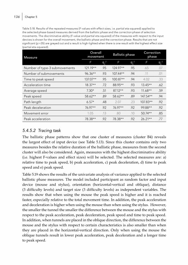
Chapter 5136
Table 5.18. Results of the repeated measures (F-values with effect sizes, i.e. partial eta-squared) applied to the selected phase-based measures derived from the ballistic phase and the correction phase of selection movements. The discriminative ability (F-value and partial eta-squared) of the measures with respect to the input devices is shown for the overall movement, the ballistic phase and the correction phase. Results that are not significant (p>.05) are greyed out and a result is high-lighted when there is one result with the highest effect size (partial eta-squared).
MeasureOverall
movement Ballistic phase Correction phase
F ηp2 F ηp
2 F ηp2
Number of type-3 submovements 121.19** .95 124.97** .95 .65 .07
Number of submovements 96.36** .93 107.44** .94 .11 .01
Time to peak speed 137.07** .95 100.87** .94 4.02 .33
Acceleration time 18.37** .72 88.95** .93 13.45** .62
Average speed 7.30* .51 87.12** .93 11.68** .59
Peak speed 58.62** .89 58.62** .89 147.54** .94
Path length 6.57* .48 2.07 .23 107.83** .92
Peak deceleration 76.97** .92 76.97** .92 99.88** .92
Movement error 1.05 .13 .80 .10 50.74** .85
Peak acceleration 78.38** .92 78.38** .92 26.21** .77
5.4.5.2 Tracing taskThe ballistic phase patterns show that one cluster of measures (cluster B4) reveals the largest effect of input device (see Table 5.13). Since this cluster contains only two measures besides the relative duration of the ballistic phase, measures from the second cluster will also be considered. Again, measures with the highest discriminative ability (i.e. highest F-values and effect sizes) will be selected. The selected measures are: a) relative time to peak speed, b) peak acceleration, c) peak deceleration, d) time to peak speed and e) peak speed.
Table 5.19 shows the results of the univariate analysis of variance applied to the selected ballistic phase measures. The model included participant as random factor and input device (mouse and stylus), orientation (horizontal-vertical and oblique), distance (3 difficulty levels) and target size (3 difficulty levels) as independent variables. The results show that when using the mouse the peak speed is higher and it is reached faster, especially relative to the total movement time. In addition, the peak acceleration and deceleration is higher when using the mouse than when using the stylus. However, the smaller the tunnel the smaller the difference between the mouse and the stylus with respect to the peak acceleration, peak deceleration, peak speed and time to peak speed. In addition, when tunnels are placed in the oblique direction, the difference between the mouse and the stylus with respect to certain characteristics is also smaller than when they are placed in the horizontal-vertical direction. Only when using the mouse the oblique tunnels result in lower peak acceleration, peak deceleration and a longer time to peak speed.
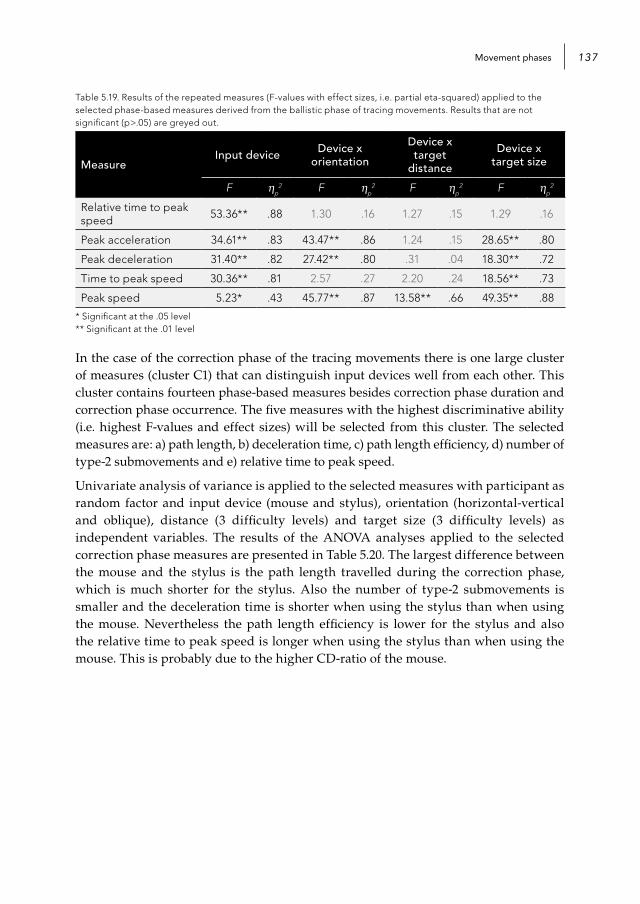
Movement phases 137
Table 5.19. Results of the repeated measures (F-values with effect sizes, i.e. partial eta-squared) applied to the selected phase-based measures derived from the ballistic phase of tracing movements. Results that are not significant (p>.05) are greyed out.
MeasureInput device Device x
orientation
Device xtarget
distance
Device xtarget size
F ηp2 F ηp
2 F ηp2 F ηp
2
Relative time to peak speed 53.36** .88 1.30 .16 1.27 .15 1.29 .16
Peak acceleration 34.61** .83 43.47** .86 1.24 .15 28.65** .80
Peak deceleration 31.40** .82 27.42** .80 .31 .04 18.30** .72
Time to peak speed 30.36** .81 2.57 .27 2.20 .24 18.56** .73
Peak speed 5.23* .43 45.77** .87 13.58** .66 49.35** .88
* Significant at the .05 level** Significant at the .01 level
In the case of the correction phase of the tracing movements there is one large cluster of measures (cluster C1) that can distinguish input devices well from each other. This cluster contains fourteen phase-based measures besides correction phase duration and correction phase occurrence. The five measures with the highest discriminative ability (i.e. highest F-values and effect sizes) will be selected from this cluster. The selected measures are: a) path length, b) deceleration time, c) path length efficiency, d) number of type-2 submovements and e) relative time to peak speed.
Univariate analysis of variance is applied to the selected measures with participant as random factor and input device (mouse and stylus), orientation (horizontal-vertical and oblique), distance (3 difficulty levels) and target size (3 difficulty levels) as independent variables. The results of the ANOVA analyses applied to the selected correction phase measures are presented in Table 5.20. The largest difference between the mouse and the stylus is the path length travelled during the correction phase, which is much shorter for the stylus. Also the number of type-2 submovements is smaller and the deceleration time is shorter when using the stylus than when using the mouse. Nevertheless the path length efficiency is lower for the stylus and also the relative time to peak speed is longer when using the stylus than when using the mouse. This is probably due to the higher CD-ratio of the mouse.

Chapter 5138
Table 5.20. Results of the repeated measures (F-values with effect sizes, i.e. partial eta-squared) applied to the selected phase-based measures derived from the correction phase of tracing movements. Results that are not significant (p>.05) are greyed out.
MeasureInput device Device x
orientation
Device xtarget
distance
Device xtarget size
F ηp2 F ηp
2 F ηp2 F ηp
2
Path length 318.78** .98 .41 .06 12.86** .66 .57 .08
Deceleration time 174.93** .96 .02 .00 6.27* .48 4.51* .41
Path length efficiency 161.78** .96 .06 .01 .57 .08 .27 .04
Type-2 submovements 88.85** .92 .53 .08 3.24 .33 7.14** .51
Relative time to peak speed 87.75** .91 .94 .14 .76 .10 3.83* .37
* Significant at the .05 level** Significant at the .01 level
The interaction effects between input device and target distance show that when the tunnel becomes longer the difference in path length and deceleration time between the mouse and the stylus becomes larger. This is mainly caused by the poorer mouse performance. In the case of the interaction effect between input device and target size the difference between the mouse and the stylus becomes larger when the tunnel width becomes smaller. Only in the case of the number of type-2 submovements there is a clear trend showing that the smaller tunnel width results in more type-2 submovements when using the mouse and in less type-2 submovements when using the stylus.
Table 5.21. Results of the repeated measures (F-values with effect sizes, i.e. partial eta-squared) applied to the selected phase-based measures derived from the ballistic phase and the correction phase of tracing movements. The discriminative ability (F-value and partial eta-squared) of the measures with respect to the input devices is shown for the overall movement, the ballistic phase and the correction phase. Results that are not significant (p>.05) are greyed out and a result is high-lighted when there is one result with the highest effect size (partial eta-squared).
MeasureOverall
movement Ballistic phase Correction phase
F ηp2 F ηp
2 F ηp2
Relative time to peak speed 91.41** .93 53.36** .88 87.75** .91
Peak acceleration 34.61** .83 34.61** .83 1.73 .20
Peak deceleration 31.38** .82 31.38** .82 35.94** .82
Time to peak speed 28.48** .80 30.36** .81 8.03* .51
Peak speed 5.23* .43 5.23* .43 44.66** .86
Path length 173.61** .96 170.64** .96 318.78** .98
Deceleration time 1.443 .17 .27 .04 174.93** .96
Path length efficiency 32.44** .82 1.32 .16 161.78** .96
Number of type-2 submovements .38 .05 .39 .05 88.85** .92

Movement phases 139
Table 5.21 shows a comparison of how well measures applied to the overall movement, the ballistic phase and the correction phase can discriminate between input devices. The applied measures are a combination of the measures selected to describe the ballistic phase (see Table 5.19) and the correction phase (see Table 5.20). As mentioned in the previous section, point measurements such as peak speed, peak acceleration and peak deceleration, are the same for the overall movement and the ballistic phase. Also in the case of the tracing task the discriminative ability of more than half of the selected phase based measures, either characterizing the ballistic phase or the correction phase, is higher than that of the overall movement measures (see Table 5.21). Only in one case a measure characterizing the overall movements shows a higher discriminative ability than when characterizing one of the movement phases, namely the relative time to peak speed. Again these results show that the division of movements into movement phases results, for certain measures, in a higher discriminative ability between input devices.
5.5 Conclusion & discussionThe main goal of this chapter was to further explore the quality of interaction movements by dividing them into smaller parts. In order to do so, we first developed a method to divide movements into five movement phases which we believed was more intuitive than the previously proposed division methods. By characterizing the ballistic phase (i.e. approach towards the target) and the correction phase (i.e. final correction towards the target) by means of position-based and velocity-based measures we wanted to acquire a more detailed description of the movement execution. Below we will describe and discuss the conclusions with respect to the questions posed in Section 5.4.1.
Are the frequency of occurrence and the duration of the various movement phases able to reveal different patterns in the data (i.e. main and interaction effects) than the overall movement duration in the case of the selection task and the tracing task?
The overall movement time did not reveal any differences between the two input devices, especially in the case of the selection task. However, the duration of the ballistic, correction and verification phase and the occurrence of the latency, initiation, correction and verification phase were able to reveal differences between the mouse and the stylus. In the case of the selection task the ballistic phase duration was shorter when using the mouse, whereas the correction and verification phase were shorter when using the stylus. Together with the occurrence of the different phases it could be concluded that the movement initiation proceeded smoother when using the mouse (i.e. lower frequency of the latency and initiation phase). Although the target approach with a mouse was faster, it was less accurate than the stylus. This meant that in order to end up at the target area more corrections (and time) were required when using the mouse. Furthermore, the higher frequency (and durations) of the verification phase indicated that the movement termination was somewhat more difficult when using the mouse than when using the stylus.

Chapter 5140
The tracing task showed similar trends, except with respect to the duration of the ballistic phase which did not display a significant difference between the mouse and the stylus. However, the relative duration of the ballistic phase did show a significant main effect of input device, indicating that relative measures should preferably be used to characterize the time intervals of the movement phases. Although the trends with respect to the movement phase occurrence were similar, a comparison between selection task and the tracing task also revealed considerable differences between the tasks in the way movements were executed. During the selection task the latency phase and the initiation phase occured more often than during the tracing task, especially when using the stylus. Also the correction phase occured more often during the selection task than during the tracing task. A possible explanation could be that the requirements of the tracing task might have resulted in a better planning of the ballistic phase, resulting in a lower frequency of the latency, initiation and correction phase.
These findings demonstrated that the characterizations of the movement phases by means of duration and occurrence provided insights that could not be obtained from the analysis of the overall movement times. The latency and initiation phase occurrence was not always high enough to characterize these phases by means of time, position-based or velocity-based measures. However, the identification of these phases resulted in a better definition of the ballistic and correction phase. As a result, the characterizations of the ballistic and correction phase by means of the time, position-based and velocity-based measures were more accurate.
What patterns (main and interaction effects) do phase-based measures reveal and are they different from the aspects already captured by the phase duration and phase occurrence measures in the case of the selection task and the tracing task?
With regard to the selection task the duration and relative duration of the ballistic phase belonged to the same cluster, which was also the case for the occurrence, duration and relative duration of the correction phase. As a result, all the other identified clusters of phase-based measures revealed additional aspects of the movement execution besides the ones already revealed by the occurrence and duration measures. The increase in the number of identified clusters showed that complementary information was provided by the phase-based measures.
With regard to the tracing task the phase-based measures were more likely to reveal the same patterns or trends as the duration and occurrence measures, especially in the case of the correction phase. This was because the duration and relative duration of the ballistic phase belonged to two separate clusters of measures, which was also the case for the occurrence, duration and relative duration of the correction phase. As a result, only one cluster of correction phase measures was able to reveal additional patterns in the data. In the case of the ballistic phase, there were two clusters of measures that were able to reveal additional patterns in the data. Nevertheless, the phase-based measures could provide more detailed insights into the identified trends, especially with respect to the differences between the two input devices.
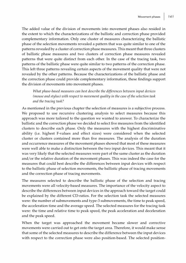
Movement phases 141
The added value of the division of movements into movement phases also resided in the extent to which the characterizations of the ballistic and correction phase provided complementary information. Only one cluster of measures characterizing the ballistic phase of the selection movements revealed a pattern that was quite similar to one of the patterns revealed by a cluster of correction phase measures. This meant that three clusters of ballistic phase measures and two clusters of correction phase measures revealed patterns that were quite distinct from each other. In the case of the tracing task, two patterns of the ballistic phase were quite similar to two patterns of the correction phase. This left three patterns revealing certain aspects of the movement quality that were not revealed by the other patterns. Because the characterizations of the ballistic phase and the correction phase could provide complementary information, these findings support the division of movements into movement phases.
What phase-based measures can best describe the differences between input devices (mouse and stylus) with respect to movement quality in the case of the selection task and the tracing task?
As mentioned in the previous chapter the selection of measures is a subjective process. We proposed to use recursive clustering analysis to select measures because this approach was more tailored to the question we wanted to answer. To characterize the ballistic and the correction phase we decided to select five measures from the identified clusters to describe each phase. Only the measures with the highest discriminative ability (i.e. highest F-values and effect sizes) were considered when the selected cluster or clusters contained more than five measures. The analysis of the duration and occurrence measures of the movement phases showed that most of these measures were well able to make a distinction between the two input devices. This meant that it was very likely that the selected measures were part of the same cluster as the duration and/or the relative duration of the movement phases. This was indeed the case for the measures that could best describe the differences between input devices with respect to the ballistic phase of selection movements, the ballistic phase of tracing movements and the correction phase of tracing movements.
The measures selected to describe the ballistic phase of the selection and tracing movements were all velocity-based measures. The importance of the velocity aspect to describe the differences between input devices in the approach toward the target could be explained by the different CD-ratios. For the selection task the selected measures were: the number of submovements and type-3 submovements, the time to peak speed, the acceleration time and the average speed. The selected measures for the tracing task were: the time and relative time to peak speed, the peak acceleration and deceleration and the peak speed.
When the target was approached the movement became slower and corrective movements were carried out to get onto the target area. Therefore, it would make sense that some of the selected measures to describe the difference between the input devices with respect to the correction phase were also position-based. The selected position-
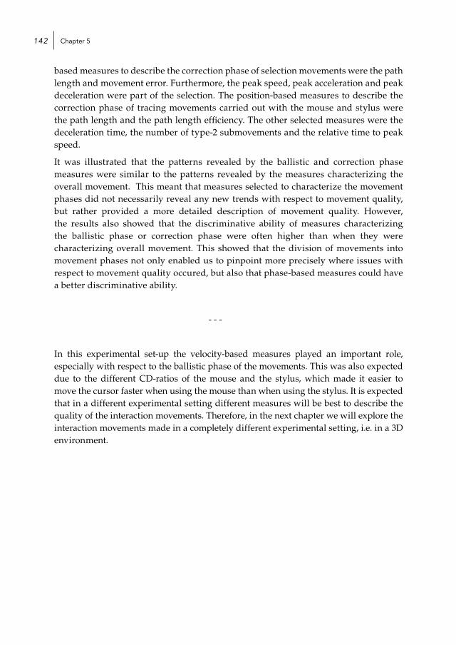
Chapter 5142
based measures to describe the correction phase of selection movements were the path length and movement error. Furthermore, the peak speed, peak acceleration and peak deceleration were part of the selection. The position-based measures to describe the correction phase of tracing movements carried out with the mouse and stylus were the path length and the path length efficiency. The other selected measures were the deceleration time, the number of type-2 submovements and the relative time to peak speed.
It was illustrated that the patterns revealed by the ballistic and correction phase measures were similar to the patterns revealed by the measures characterizing the overall movement. This meant that measures selected to characterize the movement phases did not necessarily reveal any new trends with respect to movement quality, but rather provided a more detailed description of movement quality. However, the results also showed that the discriminative ability of measures characterizing the ballistic phase or correction phase were often higher than when they were characterizing overall movement. This showed that the division of movements into movement phases not only enabled us to pinpoint more precisely where issues with respect to movement quality occured, but also that phase-based measures could have a better discriminative ability.
- - -
In this experimental set-up the velocity-based measures played an important role, especially with respect to the ballistic phase of the movements. This was also expected due to the different CD-ratios of the mouse and the stylus, which made it easier to move the cursor faster when using the mouse than when using the stylus. It is expected that in a different experimental setting different measures will be best to describe the quality of the interaction movements. Therefore, in the next chapter we will explore the interaction movements made in a completely different experimental setting, i.e. in a 3D environment.

Chapter 6
Application to 3D Environment

Chapter 6144
As mentioned in the introduction, the main goal of this thesis is to develop a methodology to quantitatively evaluate the performance of spatial input devices and interaction techniques. In the previous chapters four major components of our quantitative approach towards the evaluation of interaction movements were addressed and applied to 2D interaction movements, i.e.:
1. Applying a more optimized Fitts’ law modeling.
2. Combining begin- and endpoint, position-based and velocity-based measures.
3. Dividing movements into smaller, meaningful parts, such as movement phases.
4. Using recursive clustering analysis to select complementary measures.
In the current chapter it will be investigated how well the developed quantitative evaluation methods can be transferred to 3D interaction movements. We believe that our approach can certainly be used for the performance evaluation of simple, well-practiced 3D interaction movements. However, in the case of more complex 3D interaction tasks (especially when not well-practiced) adjustments might be necessary to be able to cope with these interaction movements in a meaningful way.
6.1 3D movementsAs mentioned in the introduction, mixed reality (MR) environments are developed to enhance the interaction with the computer interface by making it more natural (Beaudouin-Lafon, 2000; van Dam, 1997). These interaction styles are considered more intuitive because they let people apply their existing skills from interacting with everyday objects in the real world. However, this does not automatically mean that interaction movements in these MR environments are as fast, as efficient or as smooth as movements in the real world. Moving around in a virtual environment or moving objects in a virtual environment is still quite different from moving around and interacting with objects in the real world. Bowman, Kruijff, LaViola and Poupyrev (2004) described that 3D interaction in a virtual world is more difficult because “the physical world contains many more cues for understanding and constraints and affordances for action that cannot currently be represented accurately in a computer simulation”. As a result, performance in 3D virtual environments is as yet lagging behind compared to the performance in the real world (Liu, van Liere, Nieuwenhuizen, & Martens, 2009; Nieuwenhuizen, Liu, van Liere, & Martens, 2009b).
Basic movements made in real life and in 2D computer environments have the characteristics of goal-directed movements. It was shown in the previous chapter that these goal-directed movements can be divided into movement phases, which enables us to pinpoint more precisely where issues with respect to movement quality occur. However, this approach of dividing interaction movements into movement phases is only meaningful when these interaction movements are indeed goal-directed. The study in which we compared movements made in the real world and in a 3D virtual world showed that also simple 3D selection movements can be goal-directed in nature (Liu et al., 2009;

Application to 3D environment 145
Nieuwenhuizen et al., 2009b). However, when considering a more challenging 3D task, such as the ball-and-tunnel task described in Section 2.3.2, a preliminary inspection of the data shows that these interactions mainly consist of multiple successive movement intervals1 instead of one goal-directed movement interval. This means that a different approach towards attaining more detailed information from interaction movements is needed.
6.1.1 Movement intervalsFigure 6.1 shows an example of a steering movement (of average duration and with an average number of movement intervals) from the ball-and-tunnel task described in Section 2.3.2. This figure shows that the velocity profile does not have the characteristics of a typical goal-directed movement, in which the ballistic movement is programmed to reach the target location and the unintended errors are corrected during the correction phase. Instead, the steering movement consists of multiple successive movement intervals, varying in duration and traveled distance. The velocity profile of the steering movement in Figure 6.1 clearly illustrates that it is not meaningful to divide this kind of interaction movements into different movement phases.
Figure 6.1. Example of a steering movement of average duration and with an average number of movement intervals.
1 Movement intervals are intervals between pauses in which the cursor or pointer’s speed exceeds 0.02 times the movement’s peak speed.
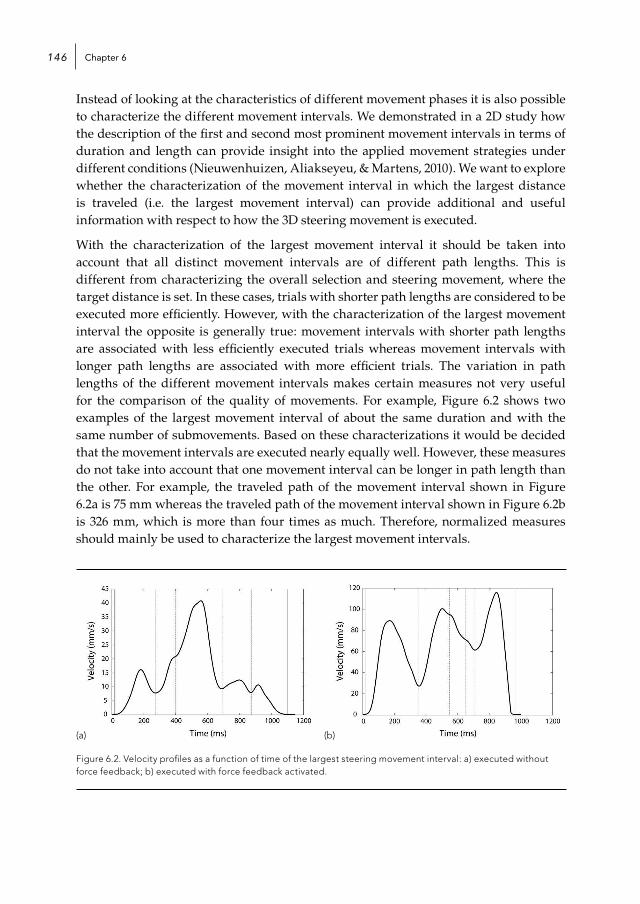
Chapter 6146
Instead of looking at the characteristics of different movement phases it is also possible to characterize the different movement intervals. We demonstrated in a 2D study how the description of the first and second most prominent movement intervals in terms of duration and length can provide insight into the applied movement strategies under different conditions (Nieuwenhuizen, Aliakseyeu, & Martens, 2010). We want to explore whether the characterization of the movement interval in which the largest distance is traveled (i.e. the largest movement interval) can provide additional and useful information with respect to how the 3D steering movement is executed.
With the characterization of the largest movement interval it should be taken into account that all distinct movement intervals are of different path lengths. This is different from characterizing the overall selection and steering movement, where the target distance is set. In these cases, trials with shorter path lengths are considered to be executed more efficiently. However, with the characterization of the largest movement interval the opposite is generally true: movement intervals with shorter path lengths are associated with less efficiently executed trials whereas movement intervals with longer path lengths are associated with more efficient trials. The variation in path lengths of the different movement intervals makes certain measures not very useful for the comparison of the quality of movements. For example, Figure 6.2 shows two examples of the largest movement interval of about the same duration and with the same number of submovements. Based on these characterizations it would be decided that the movement intervals are executed nearly equally well. However, these measures do not take into account that one movement interval can be longer in path length than the other. For example, the traveled path of the movement interval shown in Figure 6.2a is 75 mm whereas the traveled path of the movement interval shown in Figure 6.2b is 326 mm, which is more than four times as much. Therefore, normalized measures should mainly be used to characterize the largest movement intervals.
(a) (b)
Figure 6.2. Velocity profiles as a function of time of the largest steering movement interval: a) executed without force feedback; b) executed with force feedback activated.
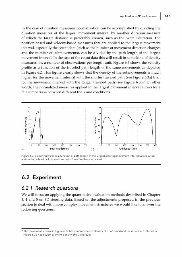
Application to 3D environment 147
In the case of duration measures, normalization can be accomplished by dividing the duration measures of the largest movement interval by another duration measure of which the target distance is preferably known, such as the overall duration. The position-based and velocity-based measures that are applied to the largest movement interval, especially the count data (such as the number of movement direction changes and the number of submovements), can be divided by the path length of the largest movement interval. In the case of the count data this will result in some kind of density measures, i.e. a number of observations per length unit. Figure 6.3 shows the velocity profile as a function of the traveled path length of the same movements as depicted in Figure 6.2. This figure clearly shows that the density of the submovements is much higher for the movement interval with the shorter traveled path (see Figure 6.3a) than for the movement interval with the longer traveled path (see Figure 6.3b)2. In other words, the normalized measures applied to the largest movement interval allows for a fair comparison between different trials and conditions.
(a) (b)
Figure 6.3. Velocity profiles as a function of path length of the largest steering movement interval: a) executed without force feedback; b) executed with force feedback activated.
6.2 Experiment
6.2.1 Research questionsWe will focus on applying the quantitative evaluation methods described in Chapter 3, 4 and 5 on 3D steering data. Based on the adjustments proposed in the previous section to deal with more complex movement structures we would like to answer the following questions:
2 The movement interval in Figure 6.3a has a submovement density of 0.067 (5/75) and the movement interval in Figure 6.3b has a submovement density of 0.015 (5/326).
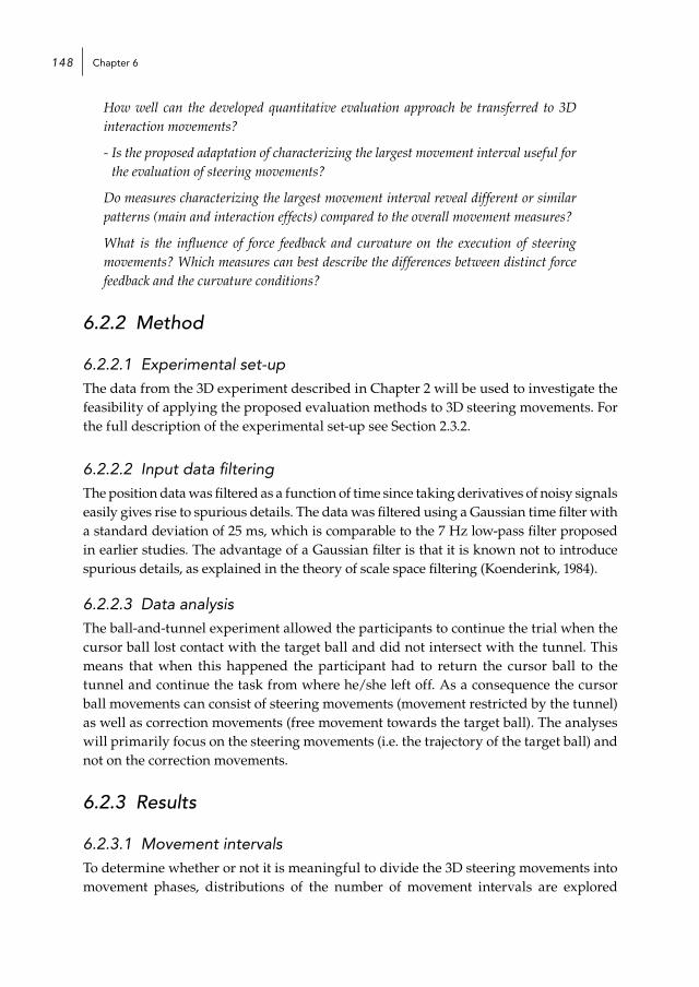
Chapter 6148
How well can the developed quantitative evaluation approach be transferred to 3D interaction movements?
- Is the proposed adaptation of characterizing the largest movement interval useful for the evaluation of steering movements?
Do measures characterizing the largest movement interval reveal different or similar patterns (main and interaction effects) compared to the overall movement measures?
What is the influence of force feedback and curvature on the execution of steering movements? Which measures can best describe the differences between distinct force feedback and the curvature conditions?
6.2.2 Method
6.2.2.1 Experimental set-upThe data from the 3D experiment described in Chapter 2 will be used to investigate the feasibility of applying the proposed evaluation methods to 3D steering movements. For the full description of the experimental set-up see Section 2.3.2.
6.2.2.2 Input data filtering The position data was filtered as a function of time since taking derivatives of noisy signals easily gives rise to spurious details. The data was filtered using a Gaussian time filter with a standard deviation of 25 ms, which is comparable to the 7 Hz low-pass filter proposed in earlier studies. The advantage of a Gaussian filter is that it is known not to introduce spurious details, as explained in the theory of scale space filtering (Koenderink, 1984).
6.2.2.3 Data analysisThe ball-and-tunnel experiment allowed the participants to continue the trial when the cursor ball lost contact with the target ball and did not intersect with the tunnel. This means that when this happened the participant had to return the cursor ball to the tunnel and continue the task from where he/she left off. As a consequence the cursor ball movements can consist of steering movements (movement restricted by the tunnel) as well as correction movements (free movement towards the target ball). The analyses will primarily focus on the steering movements (i.e. the trajectory of the target ball) and not on the correction movements.
6.2.3 Results
6.2.3.1 Movement intervalsTo determine whether or not it is meaningful to divide the 3D steering movements into movement phases, distributions of the number of movement intervals are explored
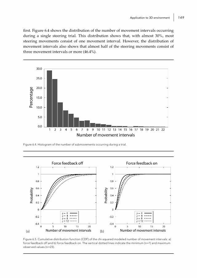
Application to 3D environment 149
first. Figure 6.4 shows the distribution of the number of movement intervals occurring during a single steering trial. This distribution shows that, with almost 30%, most steering movements consist of one movement interval. However, the distribution of movement intervals also shows that almost half of the steering movements consist of three movement intervals or more (46.4%).
Figure 6.4. Histogram of the number of submovements occurring during a trial.
(a) (b)
Figure 6.5. Cumulative distribution function (CDF) of the chi-squared modeled number of movement intervals: a) force feedback off and b) force feedback on. The vertical dotted lines indicate the minimum (n=1) and maximum observed values (n=23).
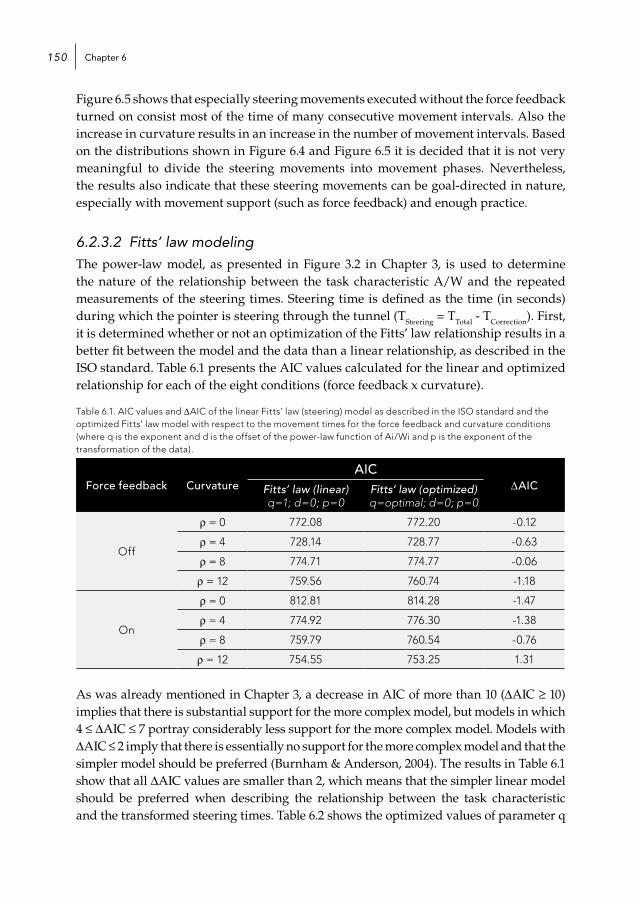
Chapter 6150
Figure 6.5 shows that especially steering movements executed without the force feedback turned on consist most of the time of many consecutive movement intervals. Also the increase in curvature results in an increase in the number of movement intervals. Based on the distributions shown in Figure 6.4 and Figure 6.5 it is decided that it is not very meaningful to divide the steering movements into movement phases. Nevertheless, the results also indicate that these steering movements can be goal-directed in nature, especially with movement support (such as force feedback) and enough practice.
6.2.3.2 Fitts’ law modelingThe power-law model, as presented in Figure 3.2 in Chapter 3, is used to determine the nature of the relationship between the task characteristic A/W and the repeated measurements of the steering times. Steering time is defined as the time (in seconds) during which the pointer is steering through the tunnel (TSteering = TTotal - TCorrection). First, it is determined whether or not an optimization of the Fitts’ law relationship results in a better fit between the model and the data than a linear relationship, as described in the ISO standard. Table 6.1 presents the AIC values calculated for the linear and optimized relationship for each of the eight conditions (force feedback x curvature).
Table 6.1. AIC values and ΔAIC of the linear Fitts’ law (steering) model as described in the ISO standard and the optimized Fitts’ law model with respect to the movement times for the force feedback and curvature conditions (where q is the exponent and d is the offset of the power-law function of Ai/Wi and p is the exponent of the transformation of the data).
Force feedback CurvatureAIC
ΔAICFitts’ law (linear) q=1; d=0; p=0
Fitts’ law (optimized) q=optimal; d=0; p=0
Off
ρ = 0 772.08 772.20 -0.12
ρ = 4 728.14 728.77 -0.63
ρ = 8 774.71 774.77 -0.06
ρ = 12 759.56 760.74 -1.18
On
ρ = 0 812.81 814.28 -1.47
ρ = 4 774.92 776.30 -1.38
ρ = 8 759.79 760.54 -0.76
ρ = 12 754.55 753.25 1.31
As was already mentioned in Chapter 3, a decrease in AIC of more than 10 (ΔAIC ≥ 10) implies that there is substantial support for the more complex model, but models in which 4 ≤ ΔAIC ≤ 7 portray considerably less support for the more complex model. Models with ΔAIC ≤ 2 imply that there is essentially no support for the more complex model and that the simpler model should be preferred (Burnham & Anderson, 2004). The results in Table 6.1 show that all ΔAIC values are smaller than 2, which means that the simpler linear model should be preferred when describing the relationship between the task characteristic and the transformed steering times. Table 6.2 shows the optimized values of parameter q

Application to 3D environment 151
together with the 95% confidence interval. These results show that the optimized power values q are not very well defined and that the value q=1, indicating a linear relationship, lies well within the confidence intervals. These results confirm the conclusion based on the ΔAIC values that a linear relationship should be preferred.
Table 6.2. Optimized values of parameter q with 95% confidence intervals as a function of the force feedback for the modeling of the 3D steering times.
Force Feedback Curvature q95% Confidence Interval
Lower bound Upper bound
Off
ρ = 0 -0.58 -3.08 1.74
ρ = 4 -0.28 -2.54 1.91
ρ = 8 -0.45 -2.73 1.65
ρ = 12 0.10 -1.93 2.16
On
ρ = 0 -0.10 -3.51 3.22
ρ = 4 -0.12 -3.17 2.92
ρ = 8 -0.35 -2.89 2.13
ρ = 12 -1.07 -3.94 1.17
Figure 6.6 shows the linear relationships between the task characteristic (A/W) and the logarithmically transformed steering times for each of the eight conditions (force feedback x curvature). This figure clearly shows that force feedback results in a better performance, indicated by the lower offset and gain values. Furthermore, it is shown that an increase in curvature of the tunnel results in lower performance levels. The difference between the various curvatures is larger for the condition in which force feedback was absent than in the condition in which the force feedback was present.
(a) (b)
Figure 6.6. Relation of the logarithmically transformed steering time to the task characteristic (A/W): (a) for the condition without force feedback and (b) for the condition with force feedback.

Chapter 6152
For each participant the performance rate (as presented in Chapter 3, Equation 3.12 and 3.13) as well as throughput (1/b) were derived from the individually optimized linear relationships. Subsequently, repeated measures analyses with force feedback and curvature as within-subjects factor were applied to the performance rate and throughput values. The results of the repeated measures analyses are presented in Table 6.3. These results show that both measures reveal significant main effects of force feedback and curvature and a significant interaction effect between force feedback and curvature. Participants perform better when they experience force feedback and when the tunnels have a low curvature. Furthermore, the results in Table 6.3 show that the performance rate has larger effect sizes than throughput, indicating a higher discriminative ability.
Table 6.3. Results of the repeated measures (F-values with effect sizes, i.e. partial eta-squared) applied to the performance rate and throughput (calculated after transformation of the effective steering time data).
Performance rate Throughput (1/b)
F(1,13) ηp2 F(1,13) ηp
2
Force feedback 79.27** .86 58.84** .82
Curvature 66.15** .84 8.37** .39
Force feedback x curvature 49.62** .79 5.20** .29** Significant at the .01 level
6.2.3.3 Steering time and errorAs mentioned in Chapter 4, the measures that are most often derived from the recorded interaction movements are time and error. Therefore, we first want to identify significant main and interaction effects (or ‘patterns’) that are present in these two measures by means of repeated measures analyses. The repeated measures analyses include force feedback (on and off), curvature (ρ = 0, ρ = 4, ρ = 8 and ρ = 12), tunnel length (240 mm, 300 mm and 360 mm) and tunnel width (30 mm and 40 mm) as within-subjects factors. Before the repeated measures analyses are carried out, a logarithmic transformation is applied to the steering time3 data and an optimal transformation (p=.28) is applied to the number of errors (i.e. steering error).
Table 6.4. Results of the repeated measures (F-values with effect sizes, i.e. partial eta-squared) applied to the transformed steering time and number of errors.
TaskForce feedback Curvature Force feedback x
Curvature
F ηp2 F ηp
2 F ηp2
Steering time 178.21** .93 86.12** .87 4.73** .27
Steering error 137.66** .91 36.69** .74 2.09 .14
* Significant at the .05 level** Significant at the .01 level
3 Steering time is defined as the time (in sec) during which the pointer was steering through the tunnel (TSteering = TTotal - TCorrection)

Application to 3D environment 153
The variation in the task characteristics tunnel length and tunnel width resulted in significant main effects within steering time (F=355.83, ηp
2=.97 and F=426.87, ηp2=.97,
respectively) and steering error (F=24.05, ηp2=.65 and F=101.98, ηp
2=.89, respectively). This means that more difficult tasks, i.e. longer and narrower tunnels, result in an increase in time and error. Since these results were intended and expected, we will focus more on the other independent variables, force feedback and curvature, when discussing the remaining results.
The results with respect to the force feedback and curvature are shown in Table 6.4, which includes the F-values as well as the effect size (partial eta-squared). Both steering time and steering error show significant main effects of force feedback and curvature. This means that force feedback enables users to move faster and make fewer errors. On the other hand, users need more time and make more errors when they have to steer through paths with a stronger curvature (see Table 6.5). The interaction effect between force feedback and curvature is only significant for steering time, although the effect size is rather small. The benefit of force feedback increases when curvature increases.
Table 6.5. Mean values of the original data and the transformed data for each level of force feedback and curvature.
MeasureForce
feedback Curvature
Off On ρ = 0 ρ = 4 ρ = 8 ρ = 12
Steering timeM (Original) 4.56 1.96 2.63 3.06 3.45 3.89
M (Transf.) 7.81 4.42 5.26 5.90 6.36 6.94
Nr of errorsM (Original) 4.05 1.30 1.48 2.39 2.95 3.88
M (Transf.) 11.33 6.46 6.67 8.46 9.64 10.81
6.2.3.4 Movement descriptionAs mentioned in Section 6.2.2.3, the analyses will primarily focus on the steering movements (i.e. the trajectory of the target ball) and not on the correction movements. This means that the position data of the target ball is analyzed instead of the position data of the cursor ball. Because the path of the target ball is fixed (the tunnel is of the same width as the target ball), most position-based measures cannot be derived from the position data, except for the path length and path length efficiency measures. The continuous and discrete measures to characterize the overall movements are presented in Table 1 and Table 2 of Appendix A.4. Besides the overall measures we also selected several duration measures, position-based measures and velocity-based measures to characterize the largest movement interval (see Table 3, Table 4 and Table 5 of Appendix A.4, respectively). As proposed in the introduction most of these measures to characterize the largest movement interval are normalized.
Recursive clustering analysis is applied to the steering measures described in Appendix A.4, together with steering time and steering error (i.e. number of errors). The recursive

Chapter 6154
clustering analysis reveals two clusters within the steering measures. Table 6.6 shows the two clusters together with the Cronbach’s Alpha, the correlations of the measures with the corresponding pattern (R-values) and the corresponding P-values4. The internal consistency of both clusters is very high, shown by the large Cronbach’s alpha values (=.99). Many measures show a good fit with the cluster they are appointed to: 27 out of 32 measures have an R-value larger than .90. The correlations show that two measures do not really fit well within the second cluster, namely the relative time to peak speed (R=.59) and the path length of the largest movement (R=.55). The clustering of measures shows that the first cluster primarily contains measures that are related to the efficiency of the overall movement (e.g. the number of errors and movement intervals and the steering efficiency) and the largest movement interval (e.g. the relative duration and path length of and before the largest movement). The second cluster mainly contains measures that are related to velocity of the executed movement and its course (e.g. the average and peak speed and the occurrence of submovements).
Table 6.6. Clustering of the measures according to the patterns identified with the 1D recursive clustering analysis of the 3D steering measures (OM = overall movement and LM = largest movement).
Cluster 1(Cronbach’s Alpha = .99)
Cluster 2(Cronbach’s Alpha = .99)
Measure R P Measure R P
Time to LM .98 .04 LM average speed .99 .05
Nr of errors .98 .05 Density nr of submovements .98 .06
Nr of movement intervals (type-1) .98 .05 Peak speed (LM) .98 .06
Nr of pauses .98 .05 OM average speed .98 .06
Relative duration of LM .97 .06 Density nr of type-2 submovements .98 .06
Relative path length of LM .97 .07 Peak deceleration (LM) .98 .07
Steering efficiency .97 .07 Steering time .96 .07
Pause occurrence .95 .06 Peak acceleration (LM) .96 .10
Relative path length before LM .94 .08 OM Acceleration time .95 .08
Path length before LM .94 .08 Relative acceleration time .95 .08
Relative steering time .93 .10 LM ratio acceleration-deceleration time .95 .09
Error occurrence .92 .07 OM nr of submovements .95 .09
Ratio correction-steering time .89 .11 OM ratio acceleration-deceleration time .94 .10
Relative time to LM .87 .12 OM nr of type-2 submovements .93 .10
Density nr of type-3 submovements .91 .12
OM nr of type-3 submovements .89 .11
Relative time to peak speed .59 .21
LM path length .55 .26
4 P-value is the ratio between the error and the variation in the data. Lower P-values indicate a measure with more discriminative power (higher signal-to-noise ratio).

Application to 3D environment 155
(a) (b)
Figure 6.7. Two 1D patterns identified by recursive clustering analysis as a function of the 48 conditions (2 force feedback settings x 4 curvatures x 2 tunnel widths x 3 tunnel lengths).
Figure 6.7 shows the two identified patterns with respect to the steering measures as a function of the 48 conditions (2 force feedback settings x 4 curvatures x 2 tunnel widths x 3 tunnel lengths). The first thing to notice from these graphs is that the differences between the two patterns are rather limited. Nevertheless, the second pattern seems to be somewhat better able to make a distinction between the two force feedback conditions also due to a lower level of variance. On the other hand, the first pattern seems to be slightly better at distinguishing between the four curvature conditions.
Univariate analysis of variance (ANOVA) was applied to the standardized values of the two identified patterns to investigate the nature of these patterns. Due to the lack of degrees of freedom, only the main effects of the independent variables (force feedback, curvature, tunnel length and tunnel width) and the 2-way interactions are included in the ANOVA model. The results of these ANOVA analyses are presented in Table 6.7 and confirm the effects seen in Figure 6.7. The results in this table show that both patterns are very well able to discriminate between the two force feedback conditions and the four curvature conditions. The effect sizes show that, in general, measures from the first cluster are somewhat better in discriminating between the curvature conditions and measures from the second cluster are somewhat better in discriminating between the force feedback conditions. Furthermore, the first pattern seems to be able to discriminate better between the different tunnel lengths and the second pattern between the different tunnel widths. Overall, the difference between the nature of the first and the second pattern is fairly limited.
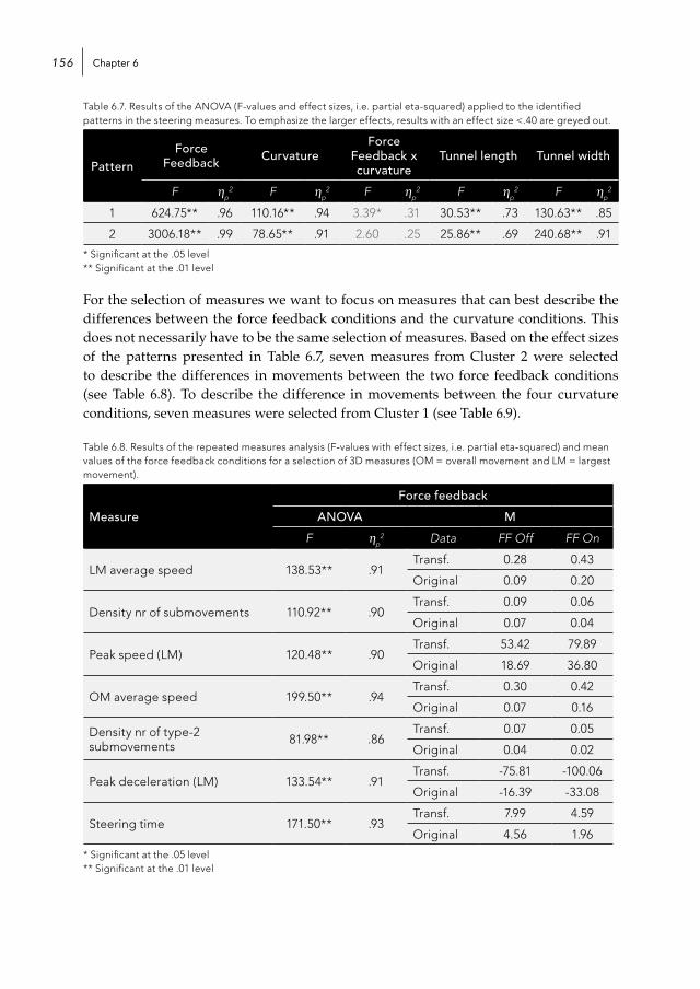
Chapter 6156
Table 6.7. Results of the ANOVA (F-values and effect sizes, i.e. partial eta-squared) applied to the identified patterns in the steering measures. To emphasize the larger effects, results with an effect size <.40 are greyed out.
PatternForce
Feedback CurvatureForce
Feedback x curvature
Tunnel length Tunnel width
F ηp2 F ηp
2 F ηp2 F ηp
2 F ηp2
1 624.75** .96 110.16** .94 3.39* .31 30.53** .73 130.63** .85
2 3006.18** .99 78.65** .91 2.60 .25 25.86** .69 240.68** .91
* Significant at the .05 level** Significant at the .01 level
For the selection of measures we want to focus on measures that can best describe the differences between the force feedback conditions and the curvature conditions. This does not necessarily have to be the same selection of measures. Based on the effect sizes of the patterns presented in Table 6.7, seven measures from Cluster 2 were selected to describe the differences in movements between the two force feedback conditions (see Table 6.8). To describe the difference in movements between the four curvature conditions, seven measures were selected from Cluster 1 (see Table 6.9).
Table 6.8. Results of the repeated measures analysis (F-values with effect sizes, i.e. partial eta-squared) and mean values of the force feedback conditions for a selection of 3D measures (OM = overall movement and LM = largest movement).
Measure
Force feedback
ANOVA M
F ηp2 Data FF Off FF On
LM average speed 138.53** .91Transf. 0.28 0.43
Original 0.09 0.20
Density nr of submovements 110.92** .90Transf. 0.09 0.06
Original 0.07 0.04
Peak speed (LM) 120.48** .90Transf. 53.42 79.89
Original 18.69 36.80
OM average speed 199.50** .94Transf. 0.30 0.42
Original 0.07 0.16
Density nr of type-2 submovements 81.98** .86
Transf. 0.07 0.05
Original 0.04 0.02
Peak deceleration (LM) 133.54** .91Transf. -75.81 -100.06
Original -16.39 -33.08
Steering time 171.50** .93Transf. 7.99 4.59
Original 4.56 1.96
* Significant at the .05 level** Significant at the .01 level
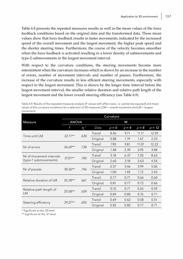
Application to 3D environment 157
Table 6.8 presents the repeated measures results as well as the mean values of the force feedback conditions based on the original data and the transformed data. These mean values show that force feedback results in faster movements, indicated by the increased speed of the overall movement and the largest movement, the higher peak speed and the shorter steering times. Furthermore, the course of the velocity becomes smoother when the force feedback is activated resulting in a lower density of submovements and type-2 submovements in the largest movement interval.
With respect to the curvature conditions, the steering movements become more intermittent when the curvature increases which is shown by an increase in the number of errors, number of movement intervals and number of pauses. Furthermore, the increase of the curvature results in less efficient steering movements, especially with respect to the largest movement. This is shown by the longer time interval before the largest movement interval, the smaller relative duration and relative path length of the largest movement and the lower overall steering efficiency (see Table 6.9).
Table 6.9. Results of the repeated measures analysis (F-values with effect sizes, i.e. partial eta-squared) and mean values of the curvature conditions for a selection of 3D measures (OM = overall movement and LM = largest movement).
Measure
Curvature
ANOVA M
F ηp2 Data ρ = 0 ρ = 4 ρ = 8 ρ = 12
Time until LM 22.11** .630Transf. 8.46 9.71 11.11 12.59
Original 0.88 1.19 1.67 2.23
Nr of errors 36.69** .738Transf. 7.90 9.81 11.07 12.22
Original 1.48 2.39 2.95 3.88
Nr of movement intervals (type-1 submovements) 37.01** .740
Transf. 5.18 6.37 7.20 8.63
Original 2.60 3.18 3.63 4.54
Nr of pauses 38.26** .746Transf. 2.57 3.46 3.99 5.06
Original 1.00 1.45 1.72 2.43
Relative duration of LM 25.38** .661Transf. 0.77 0.71 0.66 0.60
Original 0.81 0.77 0.72 0.66
Relative path length of LM 25.08** .659
Transf. 0.76 0.71 0.65 0.59
Original 0.84 0.80 0.76 0.71
Steering efficiency 29.27** .692Transf. 0.69 0.62 0.58 0.51
Original 0.85 0.80 0.77 0.71
* Significant at the .05 level** Significant at the .01 level
Chapter 6158
6.3 Conclusion & discussionThe main goal of this chapter was to explore the extensibility of the quantitative evaluation methods from 2D interaction movements to 3D interaction movements. The four components of the quantitative evaluation approach (applying the optimized Fitts’ law modeling, using different types of measures, dividing movements into smaller parts and selecting measures by cluster analysis) were applied to 3D steering movements. Below we will describe and discuss the conclusions with respect to the questions posed in Section 6.2.1.
How well can the developed quantitative evaluation approach be transferred to 3D interaction movements?
The results showed that most of the quantitative evaluation methods could be easily transferred to 3D interaction movements:
- The Fitts’ law modeling showed clear differences between the force feedback and curvature conditions. Furthermore, the measure performance rate we proposed in Chapter 3 showed a higher discriminative ability than throughput especially for showing the effect of curvature (indicated by the higher effect sizes).
- Although the set-up of the experimental task restricted the use of most position-based measures (because the path of the target ball was fixed) it was possible to apply a variety of duration, position-based and velocity-based measures to the 3D steering movements. The cluster analysis showed that the first cluster mainly consisted of (normalized) duration and position-based measures, whereas the second cluster mainly contained velocity-based measures. This showed that the velocity-based measures were able to identify different patterns within the steering data compared to the duration and position-based measures, i.e. they were complementary to each other.
- The distributions of the movement intervals showed that almost half of the steering movements consisted of three movement intervals or more. In other words, a large portion of the steering movements were not goal-directed in nature. This meant that the division of the steering movements into movement phases would not have been very meaningful. Although this particular component of the evaluation approach (dividing movements into movement phases) could not be applied to the evaluated 3D steering movements it was possible to gather additional information by characterizing the largest movement interval of each trial. The results showed that several measures characterizing the largest movement interval were selected for their ability to differentiate between the force feedback conditions or between the curvature conditions. Although the characterization of the largest movement interval provided additional information about how the steering movements were executed it was more difficult to pin-point exactly where issues with respect to movement quality occured as with the phase-based measures.
Application to 3D environment 159
- The recursive clustering analysis revealed two clusters of measures of which the first cluster was somewhat better at revealing differences between the curvature conditions and the second cluster between the force feedback conditions. As a result two sets of measures were selected that were very well able to describe the influence of force feedback and curvature on the steering movements.
What patterns (main and interaction effects) do measures characterizing the largest movement interval reveal and are they different from the aspects already captured by the overall movement measures.
The results of the recursive clustering analysis showed that the characterization of the largest movement interval did not reveal any new patterns in the data. The measures characterizing the overall movement and the largest movement interval were about equally divided over the two clusters. Both of these clusters could differentiate well between the two force feedback conditions and the four curvature conditions. The difference between the clusters could be better explained by the type of measures that were clustered together: the first cluster primarily contained measures that were related to the steering fluency and the efficiency of the overall movement and the largest movement interval and the second cluster mainly contained measures that were related to velocity of the executed movement and its course.
What is the influence of force feedback and curvature on the execution of the steering movements? Which measures can best describe the difference between the force feedback and the curvature conditions?
The patterns revealed by the recursive cluster analysis showed that the measures from Cluster 1 were somewhat better in discriminating between the four curvature conditions. As mentioned before, this cluster mainly contained measures related to the steering fluency and the efficiency of the overall movement and the largest movement interval, such as the number of errors, the number of movement intervals, the time until the largest movement interval and the relative duration and path length of the largest movement interval. The repeated measures analyses clearly showed that an increase in curvature of the tunnel resulted in steering movement that were more intermittent and that were less efficient, especially with respect to the execution of the largest movement interval.
The identified patterns showed that the measures from Cluster 2 were generally better in discriminating between the force feedback conditions. This cluster primarily contained measures related to the velocity of the steering movement and its course, such as the average speed, the peak speed, the peak deceleration, and the density and number of submovements. The repeated measures analysis showed that when the force feedback was turned on the steering movements were faster and the course of the velocity became much smoother.
The two groups of selected measures were able to describe the largest effects of force feedback and curvature on the 3D steering movements (based on the identified patterns).
Chapter 6160
This did not mean that other measures were not able to discriminate between the force feedback or curvature conditions. As the identified patterns showed, measures from both clusters were generally well able to discriminate between the force feedback and the curvature conditions.
- - -
The results of this chapter clearly showed that most components of the quantitative evaluation methods that were described in Chapter 3, 4 and 5 can be transferred to 3D interaction movements. Especially when the interaction movements are goal-directed in nature, the methods will be of great support in understanding how interaction movements are executed and in pinpointing where issues with respect to movement quality occur (i.e. during which phase of the movement). However when interaction movements are not goal-directed in nature the method of dividing movements into movement phases cannot be applied. Although we proposed to characterize the largest movement interval, further studies are necessary to determine what the best method is to abstract more detailed information from more complex interaction movements.

Chapter 7
Conclusions and future directions
Chapter 7162
7.1 Summary of contributionsAs mentioned in the introduction, movement time and error rate are often the only quantitative measures used in the evaluation of mixed reality (MR) desktop systems. In this thesis we have explored several ways to systematically abstract more detailed information from goal-directed interaction movements in order to provide a more detailed description of these movements. The main contributions of this thesis correspond to the four major components of our quantitative approach towards the evaluation of interaction movements:
1. We proposed a more general model for Fitts’ law which allows for a more precise modeling of the movement time data (see Chapter 3). Based on the optimized Fitts’ law modeling an alternative measure for throughput is proposed that takes into account the offset, gain and form of the relationship between task characteristic (A/W) and the (transformed) movement time (i.e. performance rate).
2. We showed that it is beneficial to also use more complex measures, i.e. measures that require more effort with respect to data logging and computation (such as position-based and velocity-based measures) besides movement time and error rate (see Chapter 4).
3. We proposed a method that divides movements into five movement phases in a more intuitive way (see Chapter 5). We demonstrated that the characterization of the movement phases resulted in a more detailed description of the interaction movements.
4. We demonstrated that recursive cluster analysis can be used to select complementary measures that are able to address a specific research question, such as understanding the difference between certain input devices or interaction techniques (see Chapter 4 and Chapter 5).
Throughout the iterative design process (design and re-design) these quantitative evaluation components can be applied in usability tests to gather more detailed information about the interaction movements for the purpose of comparing multiple design solutions of, for example, input devices and interaction techniques. These detailed comparative descriptions will subsequently reveal the benefits and drawbacks of the evaluated input devices or interaction techniques which can serve as input for the next re-design cycle. In Chapter 6 we showed that the different components of our evaluation approach cannot only be used in usability tests evaluating 2D computer interactions but also in usability tests evaluating 3D computer interactions. Conclusions with respect to these four major components of the evaluation approach are further addressed in the next section.

Conclusions and future directions 163
7.2 Research conclusions
7.2.1 Optimizing Fitts’ law modeling
Optimization of Fitts’ Law modeling ensures that the conclusions drawn from the results are more statistically sound (due to improved normality and homogeneity), more accurate (due to the better fit) and more convincing (due to the larger effect sizes) than conclusions drawn from the traditional Fitts’ law model as described in the ISO standard (ISO 9241-9, 2000).
The optimization of Fitts’ law modeling we proposed consists of two important elements:
- transformation of measured data, and- application of a more general Fitts’ law model.
The proposed approach towards Fitts’ law modeling also allows for a more informative summary measure which takes into account the offset, gain and form of the relationship between the task characteristic (A/W) and the (transformed) movement time (i.e. performance rate).
7.2.1.1 Data transformationExploration of the movement time data of the 2D experiment revealed issues with respect to the normality and homogeneity of the data. Especially in the case of the tracing task the movement time data was highly skewed and there was a large variation in de condition variances. It was shown that the transformation of the movement time data resulted in a large improvement with respect to the normality and the homogeneity of the data. Consequently, it is more valid to draw conclusions from parametric statistical analyses, such as linear regression analysis (i.e. Fitts’ law) because the movement time data is placed on a scale that is linearly interpretable. Not only is it more valid to interpret the Fitts’ law regression results, the discriminatory power of the summary measure throughput also increased by the transformation of the movement time data. As a result, some additional significant effects between the experimental conditions were revealed.
These results clearly show the advantages of transforming skewed and non-homogeneous data before applying parametric analysis. The advantage of the proposed approach towards data modeling is that different data transformations can be compared with each other to select the most beneficial transformation instead of just picking one. For example, the logarithmic, square root and reciprocal transformations, which according to Field (2009) are able to reduce a positive skew, can be easily compared with each other in order to select the best transformation. When applying a transformation to a data distribution it should be taken into account that the same transformation must be applied to the data of the conditions that are compared with each other (Field, 2009). This means that when different input devices are compared with each other the data of these input devices should be transformed by the same function.

Chapter 7164
7.2.1.2 Optimized Fitts’ law modelingAs mentioned before, we proposed a more general model for Fitts’ law which allows for a more precise modeling of the relationship between movement time and the task characteristic (A/W). The added value of the optimization of Fitts’ Law modeling was illustrated best by the modeling of the tracing task data: it was shown that a power-law function instead of the predetermined logarithmic function best described the relationship between the task characteristic (A/W) and the transformed tracing time. In addition, the form of the relationship between the task characteristic (A/W) and the transformed tracing time was also quite different for the four experimental conditions of input devices and movement directions.
Furthermore, the proposed measure ‘performance rate’ was better able to make a significant distinction between the different 2D input devices and movement directions, especially in the case of the selection task data. The Cohen’s d values (indicating the effect sizes) showed that the discriminability of the performance rate measure was better than that of the throughput (1/b). Also in the case of the 3D experiment the effect sizes, i.e. partial eta-squared, of the performance rate measure were higher than those of the throughput measure. This shows that the optimization of the Fitts’ law relationship and its derivative measure ‘performance rate’ allow for a better comparison between variables such as input devices and interaction techniques.
Although the performance rate measure can discern well between different experimental conditions, it should be taken into account that interaction effects of the independent variables (such as input devices or interaction techniques) with the task characteristic (A/W) are not revealed. However, a graph can illustrate possible interaction effects between the independent variables and the task characteristic. Therefore, we recommend that a summary measure like throughput or performance rate is used in combination with a graph of the Fitts’ law relationships in its complete form, as suggested by Zhai (2004).
7.2.2 Combining begin- and endpoint, position-based and velocity-based measures.
For a complete description of the effect of independent variables on the quality of interaction movements a combination of begin- and endpoint, position-based and velocity-based measures should be applied to these interaction movements.
In the case of the 2D experiment, the description of the difference between the input devices was the main focus of the data analysis. Although differences were expected, movement time was not able to reveal any differences between the input devices in both the selection and the tracing task data. Furthermore, error rate only revealed a significant difference between input devices in the case of the tracing task. The inclusion of position-based measures and subsequently velocity-based measures in the recursive

Conclusions and future directions 165
clustering analysis revealed additional patterns in the data of which some were able to discriminate well between the two input devices. The increase in the number of identified clusters showed that complementary information is provided by the position-based and the velocity-based measures. Furthermore, these results clearly illustrate that erroneous conclusions might be drawn about the difference between input devices or interaction techniques when only movement time and error rate are used as performance measures.
In the case of the 3D experiment the position-based and velocity-based measures did not reveal any additional patterns in the 3D steering data. However, the selected position-based and velocity-based measures were able to provide considerably more insight into the effect of force feedback and tunnel curvature on the execution of steering movements than the information provided by the steering time and the number of errors. The results of both the 2D and 3D experimental data show that although the position-based and velocity-based measures require more effort to derive from interaction movements (compared to movement time and error rate), the benefits with respect to the description of movement quality certainly outweigh the costs.
A disadvantage of the experimental set-up of the 3D steering task was that only a limited number of position-based measures could be derived from the steering movements, because the path was restricted. When designing experimental interaction tasks it should be determined beforehand whether the desired measures can be derived from the interaction movements in order to get a satisfactory description of the interaction movements.
7.2.3 Dividing movements into smaller, meaningful parts, such as movement phases.
Dividing movements into smaller, meaningful parts (especially goal-directed movements into movement phases) ensures a more detailed description of interaction movements, a more precise allocation of where issues with respect to movement quality occur and a higher discriminative ability of various measures compared to the overall movement measures.
The goal-directed selection and tracing movements of the 2D experiment were divided into five movement phases to gather more detailed information about the movement execution. Although the occurrence of the latency and initiation phase was not high enough to characterize these phases by means of time, position-based or velocity-based measures, the identification of these phases resulted in a better definition of the ballistic and correction phase. Consequently, the characterizations of the ballistic and correction phase by means of the time, position-based and velocity-based measures were more accurate.
The added value of dividing goal-directed movements into movement phases is clearly shown by the characterization of the various movement phases by means of their

Chapter 7166
duration and occurrence rate. In contrast to the overall movement time, the duration of the ballistic, correction and verification phase and the occurrence of the latency, initiation, correction and verification phase were able to reveal differences between the mouse and the stylus. In short, the target approach (ballistic phase) when using the mouse is relatively faster, but less accurate than with the stylus, which means that more corrections towards the target (correction phase) are required.
To further characterize the ballistic phase and the correction phase the position-based and velocity-based measures were applied to these phases when possible (i.e. phase-based measures). The recursive clustering analysis and the multi-directional scaling (MDS) showed that some of the patterns revealed by ballistic phase measures were complementary to those of the correction phase for both the selection task and the tracing task. MDS showed that some of the identified patterns were even complementary to the patterns revealed by the overall movement measures. This means that the phase-based measures cannot only provide a more detailed description of the interaction movements but they can also reveal additional effects that are present in the data. In addition, the division of movements into movement phases resulted, for certain measures, in a higher discriminative ability between input devices.
The 3D steering task showed that when the interaction movements are not goal-directed in nature, it is not meaningful to divide these movements into movement phases. These steering movements were not composed of distinctive movement phases but often of multiple, successive movement intervals. Therefore, the characterization of the largest movement interval (i.e. interval during which the largest distance was traveled) was used to gather more information about the movement quality. Although the measures characterizing the largest movement interval were not able to reveal any new patterns in the data, they do provide more detailed information about the execution of the interaction movements.
7.2.4 Using recursive clustering analysis to select measures.
Recursive clustering analysis can be used as an objective method to select measures that are able to address a specific research question, by looking at the pattern that a particular cluster of measures is able to reveal.
The main goal of the recursive clustering analysis (RCA) is to group measures in the same cluster that are more similar to each other (i.e. measures that reveal a similar underlying 1D pattern) than to those in other clusters (i.e. measures that reveal different patterns). The resultant clusters can, for example, provide valuable insight with respect to the ability of certain measures to provide complementary information. However, we showed that this clustering method can also be used to select measures in a targeted way by identifying the 1D pattern that can best discriminate between the different levels of a certain independent variable. The performance measures that are able to reveal this selected 1D pattern can subsequently provide a clear description of the main
Conclusions and future directions 167
aspects in which the interaction movements differ from each other with respect to this independent variable (e.g. the two input devices in the case of the 2D experiment and the force feedback and curvature conditions in the case of the 3D experiment).
A drawback of the proposed method is that a larger number of measures are required in order to get properly sized clusters and end up with a nice selection of measures that is able to answer the question at hand. However, it is difficult to predict the discriminability of a measure since it is highly dependent on the system (e.g. task, input device, interaction technique, environment and context) being evaluated. Although the selection method requires somewhat more effort with respect to deriving a considerable number of measures from the data, researchers are less restricted by the measures they picked beforehand without having any ideas about their discriminative ability. In order to improve the design of for example input devices or interaction techniques we are foremost interested in a description of the main aspects in which the interaction movements do differ from each other (i.e. measures that display a high discriminative ability) and not of the aspects in which the movements do not differ.
Another drawback of the proposed selection method is that the recursive clustering analysis is not included in often used software packages such as SPSS and SAS. An alternative, but more effortful, approach is to compare the effect sizes with respect to a particular independent variable (e.g. input device) which needs to be determined for each measure separately. Measures with the highest effect size can then be selected to provide a description of the most important differences between the levels of this independent variable (e.g. between the mouse and stylus).
7.3 Future directionsIn this thesis several quantitative methods are proposed to gather more detailed information about the way interaction movements are carried out. However, there are still some questions remaining with respect to (certain elements of) the proposed evaluation approach which might require further research. We will address several directions for future research, which are related to the broader application of the proposed methodology (external validity and complex interaction movements), the human aspect of the interaction (user experience and physiological measures) and the accessibility of the methodology.
7.3.1 External validityAs mentioned in the introduction, this thesis is a first step towards the development of a more thorough and standardized method for the quantitative evaluation of spatial input devices and interaction techniques used especially in mixed reality (MR) desktop systems. The initial development of the proposed methodology was based on 2D interaction movements and the method was used to evaluate a pen-based MR desktop system (with and without force feedback). We showed that the different components of our evaluation approach can be applied in usability tests evaluating elementary 3D

Chapter 7168
computer interactions. A next step would be to apply this evaluation methodology to other types of MR desktop systems, e.g. MR systems in which tangible objects are used for interaction purposes, to further improve and strengthen the methodology and to ascertain its generalizability.
Also the generalizability of the results with respect to the more general Fitts’ law model could be the focus of future research. As mentioned in Chapter 3, Fitts’ law was introduced in the HCI field in 1978 by Card et al. (1978) to compare the performance of various input devices, such as the mouse, rate controlled isometric joystick, step keys, and text keys. Since then, Fitts’ law has been frequently applied in many different HCI studies and as a result it has become a well-established model in the HCI field. Unlike the generalized Fitts’ law model we proposed, the external validity of the original Fitts’ law model has been determined over a prolonged period of time. The direct comparison of the generalized Fitts’ law model and the original Fitts’ law model (in the 2D and 3D study) clearly shows the merits of the more general Fitts’ law model. However, more research applying the generalized Fitts’ law model and the performance rate measure is essential to support the claim of external validity of the research results described in this thesis. An even more compelling comparison would be when the generalized Fitts’ law model would be applied to data sets of already reported studies, especially to the original Fitts’ law data set (Fitts, 1954).
7.3.2 Complex interaction movementsThe analysis of the 3D steering data showed that when an interaction task becomes more difficult the interaction movements become less goal-directed in nature. In these cases, the interaction movements are more a sequence of discrete movement intervals (separated by pauses) and the division of these interaction movements into movement phases becomes meaningless. In the case of more complex 3D tasks (e.g. docking tasks) and less clearly defined tasks (e.g. way-finding tasks) it will be even more the case that the interaction movements do not have the clear characteristics of simple goal-directed movements.
Instead of dividing the 3D steering movements into movement phases we characterized the largest movement interval to gather additional information about the movement execution. However, in contrast to the characterization of movement phases, the characterization of the largest movement interval was not really able to provide a clear indication of where most interaction problems occur during the movement. Furthermore, the information that is residing within the other movement intervals is discarded. Instead of comparing just the mean values of the largest movement interval, future research should explore the possibility of comparing the distributions of all movement intervals with each other. This future research should, among other things, answer the questions of what statistical analysis methods can be used best for the comparison of distributions and whether the comparison of distributions is able to provide sufficiently complementary information about the movement execution.
Conclusions and future directions 169
7.3.3 User experienceThe main goal of the methodology proposed in this thesis was to gather more detailed information from goal-directed movements by focusing on the task performance. However, it remains a question how users experienced the various computer interactions and how satisfied they were with the interaction movements they produced. User satisfaction with respect to input devices and interaction techniques has been assessed by means of an interview (MacKenzie & Jusoh, 2001) or a short questionnaire (Baudisch, Cutrell, & Robertson, 2003; Douglas, Kirkpatrick, & MacKenzie, 1999; Lapointe, 2004; Silfverberg, MacKenzie, & Kauppinen, 2001; Silva, Lyons, Kawato, & Tetsutani, 2003; see also ISO 9241-9, 2000). These short questionnaires are adapted from the ISO standard 9241-9 and mainly focus on fatigue and effort. Due to the general nature of the comfort-rating scales included in the ISO standard these questionnaires are not really able to assess the degree to which users are satisfied with the executed movements. Future research could focus more on the subjective evaluation of interaction movements which would complement the objective evaluation method proposed in this thesis.
It would not only be valuable to assess user satisfaction but also to explore how it is related to the coordination of interaction movements1. During some movements the muscles might be organized better in working together than during other movements (Malone & Crowston, 1994). In other words, some movements might be better coordinated than other movements. However, it is not exactly known what people understand by the term ‘coordination’ and what elements are important to describe coordination (e.g. to be included in a questionnaire). It would also be worthwhile to explore which aspects of movement coordination have the highest and the lowest impact on user satisfaction. Furthermore, when users are not able to produce well-coordinated movements they might also experience stress or frustration. It requires further investigation whether the level of stress experienced during system interaction can be assessed with the help of a questionnaire such as the shortened version of the State Anxiety Inventory (Bruns Alonso, Hummels, Keyson, & Hekkert, 2011; Marteau & Bekker, 1992) or the Self-Assessment-Manikin (Bradley & Lang, 1994; Thüring & Mahlke, 2007).
7.3.4 Physiological measurementsIn this thesis, the main focus was on developing a more quantitative evaluation method that can reveal “in what way” the performance of certain input devices or interaction techniques are different. Although we only focused on the resultant interaction movements in the computer environment, there is also a physical component that can inform us how interaction movements are carried out. Difference in posture or required physical effort might provide us with a deeper understanding of why certain input devices or interaction techniques are easier to use than others. As Hogan and Flash
1 Malone and Crowston (1994) defined coordination as the act of managing interdependencies between activities. Coordination can be seen as an organized working together of muscles aimed at bringing about a purposeful movement.
Chapter 7170
(1987) mentioned: “Even simple movements require the coordination of a bewildering number of muscles”. Compared to the use of a personal computer it is expected that an MR desktop system demands more extensive coordination skills and more physical effort due to the extra dimension (i.e. increase in the degrees of freedom of movement), although this is also dependent on the system and design solutions being used. In our opinion, it would be an interesting direction for future research to relate quantitative cursor movement measures to physiological measures.
One of the physiological measures that might be highly useful for this purpose is electromyography (EMG). EMG is a technique used for the evaluation and recording of the electrical activity produced by skeletal muscles. Not only the muscle activity but also the amount of local muscle fatigue can be indicated by means of surface electromyographic (sEMG) signal processing (Cifrek, Medved, Tonković, & Ostojić, 2009). Although the EMGs can be easily acquired on the surface of human skin through conveniently attachable electrodes (Ahsan, Ibrahimy, & Khalifa, 2009), the data gathering, processing and analysis of the EMG data will be more demanding than that of the pointer data. Nevertheless, the combination of these two types of data might provide invaluable insight into the execution of computer interaction movements.
Interaction with a computer system can not only result in physical stress but also in mental stress (i.e. frustration), as was also mentioned in the previous section. There are several ways to indirectly measure emotional states like frustration such as galvanic skin response, heart rate, interbeat interval, heart rate variability, blood pressure, blood volume pulse, rate of respiration and depth of breath (Picard, Vyzas, & Healey, 2001; Puri, Olson, Pavlidis, Levine, & Starren, 2005). The ongoing development of wearables might facilitate the registration of these emotion indicators in an unobtrusive way. It would be interesting to explore how the qualitative and quantitative measures of user experience can be used in combination with the pointer data to further optimize (3D) computer interactions.
7.3.5 Accessibility of methodologyThe methodology proposed in this thesis is intended to support designers and researchers of spatial input devices and interaction techniques with the evaluation and improvement of their design solutions. However, the generalized Fits’ law modeling and the recursive clustering analysis for the selection of measures require a certain level of statistical knowledge. Also the derivation of the large number of measurements requires some effort and knowledge of mathematical software packages. This might discourage designers and researchers to apply (parts of) the quantitative methodology to gather more detailed information from spatial interaction movements. Therefore, effort should not only be invested to further improve and extend the quantitative evaluation methodology but also to increase the accessibility of the methodology (also outside academia).

Conclusions and future directions 171
A possible way to lower the threshold for applying a more extensive evaluation methodology is to develop a tool in which the different components of the quantitative methodology are incorporated. For example, it would be valuable if this tool is able to support the recording of interaction movements, after which various measures are automatically derived from the registered interaction movements and clustered based on their similarity. Although it will require a considerable effort to increase the accessibility of the proposed evaluation methodology it can allow this methodology to live up to its full potential.

172

References

174
Accot, J., & Zhai, S. (1997). Beyond Fitts’ law: Models for trajectory-based HCI tasks. In Proceedings of the SIGCHI Conference on Human Factors in Computing Systems (pp. 295–302). New York, NY: ACM Press.
Accot, J., & Zhai, S. (1999). Performance evaluation of input devices in trajectory-based tasks: an application of the steering law. In Proceedings of the SIGCHI Conference on Human Factors in Computing Systems (pp. 466–472). New York, NY, USA: ACM Press.
Adam, J. J., Paas, F. G. W. C., Eyssen, I. C. J. M., Slingerland, H., Bekkering, H., & Drost, M. (1995). The control of two-element, reciprocal aiming movements: Evidence for chunking. Human Movement Science, 14(1), 1–11.
Ahlström, D. (2005). Modeling and improving selection in cascading pull-down menus using Fitts’ law, the steering law and force fields. In Proceedings of the SIGCHI Conference on Human Factors in Computing Systems (pp. 61–70). New York, NY: ACM.
Ahsan, M. R., Ibrahimy, M. I., & Khalifa, O. O. (2009). EMG signal classification for human computer interaction: A review. European Journal of Scientific Research, 33(3), 480–501.
Akamatsu, M., MacKenzie, I. S., & Hasbroucq, T. (1995). A comparison of tactile, auditory, and visual feedback in a pointing task using a mouse-type device. Ergonomics, 38(4), 816–827.
Aliakseyeu, D., Martens, J.-B., Subramanian, S., Vroubel, M., & Wesselink, W. (2001). Visual Interaction Platform. In Proceedings of the IFIP International Conference on Human-Computer Interaction (Vol. 2001, pp. 232–239).
Azen, R., & Walker, C. M. (2010). Categorical Data Analysis for the Behavioral and Social Sciences. Routledge.
Bade, R., Ritter, F., & Preim, B. (2005). Usability comparison of mouse-based interaction techniques for predictable 3d rotation. In Proceedings of the International Symposium on Smart Graphics (pp. 138–150). Springer Berlin Heidelberg.
Balakrishnan, R. (2004). “Beating” Fitts’ law: virtual enhancements for pointing facilitation. International Journal of Human-Computer Studies, 61, 857–874.
Basdogan, C., Ho, C.-H., Srinivasan, M. A., & Slater, M. (2000). An experimental study on the role of touch in shared virtual environments. ACM Transaction on Computer-Human Interaction, 7(4), 443–460.
Baudisch, P., Cutrell, E., & Robertson, G. (2003). High-density cursor: a visualization technique that helps users keep track of fast-moving mouse cursors. In Proceedings of the IFIP International Conference on Human-Computer Interaction (pp. 236–243).
References 175
Beaudouin-Lafon, M. (2000). Instrumental interaction: an interaction model for designing post-WIMP user interfaces. In Proceedings of the SIGCHI Conference on Human Factors in Computing Systems (pp. 446–453). New York, NY: ACM.
Behbehani, K., Kondraske, G. V., & Richmond, J. R. (1988). Investigations of upper extremity visuomotor control performance measures. IEEE Transactions on Biomedical Engineering, 35(7), 518–525.
Billinghurst, M., Kato, H., & Poupyrev, I. (2001). The MagicBook: a transitional AR interface. Computers & Graphics, 25(5), 745–753.
Bowman, D. A., Davis, E. T., Hodges, L. F., & Badre, A. N. (1999). Maintaining spatial orientation during travel in an immersive virtual environment. Presence: Teleoperators and Virtual Environments, 8(6), 618–631.
Bowman, D. A., & Hodges, L. F. (1999). Formalizing the design, evaluation, and application of interaction techniques for immersive virtual environments. Journal of Visual Languages & Computing, 10(1), 37–53.
Bowman, D. A., Kruijff, E., LaViola, J. J., & Poupyrev, I. (2004). 3D user interfaces: Theory and practice. Redwood City, CA, USA: Addison Wesley Longman Publishing Co., Inc.
Bradley, M. M., & Lang, P. J. (1994). Measuring emotion: The self-assessment manikin and the semantic differential. Journal of Behavior Therapy and Experimental Psychiatry, 25(1), 49–59.
Bruns Alonso, M., Hummels, C. C. M., Keyson, D. V., & Hekkert, P. P. M. (2011). Measuring and adapting behavior during product interaction to influence affect. Personal and Ubiquitous Computing, 17(1), 81–91.
Buck, L. (1980). Motor performance in relation to control-display gain and target width. Ergonomics, 23(6), 579–589.
Burnham, K. P., & Anderson, D. R. (2004). Multimodel inference: Understanding AIC and BIC in model selection. Sociological Methods & Research, 33(2), 261 –304.
Card, S. K., English, W. K., & Burr, B. J. (1978). Evaluation of mouse, rate-controlled isometric joystick, step keys, and text keys for text selection on a CRT. Ergonomics, 21(8), 601–613.
Casiez, G., Plenacoste, P., & Chaillou, C. (2004). Does DOF separation on elastic devices improve user 3D steering task performance? In Lecture notes in computer science (pp. 70–80). Springer.
Chen, J., & Bowman, D. A. (2006). Effectiveness of cloning techniques for architectural virtual environments. In Proceedings of the IEEE Conference on Virtual Reality (pp. 103–110).
176
Chen, J., Pyla, P. S., & Bowman, D. A. (2004). Testbed evaluation of navigation and text display techniques in an information-rich virtual environment. In Proceedings of the IEEE Conference on Virtual Reality (pp. 181–289).
Chittaro, L., & Scagnetto, I. (2001). Is semitransparency useful for navigating virtual environments? In Proceedings of the ACM Symposium on Virtual Reality Software and Technology (pp. 159–166). New York, NY, USA: ACM.
Cifrek, M., Medved, V., Tonković, S., & Ostojić, S. (2009). Surface EMG based muscle fatigue evaluation in biomechanics. Clinical Biomechanics, 24(4), 327–340.
Cockburn, A., Gutwin, C., & Greenberg, S. (2007). A predictive model of menu performance. In Proceedings of the SIGCHI Conference on Human Factors in Computing Systems (pp. 627–636). New York, NY: ACM Press.
Cockburn, A., & McKenzie, B. (2002). Evaluating the effectiveness of spatial memory in 2D and 3D physical and virtual environments. In Proceedings of the SIGCHI Conference on Human Factors in Computing Systems (pp. 203–210). New York, NY, USA: ACM.
Cohen, J. (1992). A power primer. Psychological Bulletin, 112(1), 155–159.
Commandeur, J. J. F., & Heiser, W. J. (1993). Mathematical derivations in the proximity scaling (PROXSCAL) of symmetric data matrices (Tech. Rep. No. RR-93-03). Leiden, The Netherlands: Department of Data Theory, Leiden University.
Crossman, E. R. F. W., & Goodeve, P. J. (1983). Feedback control of hand-movement and Fitts’ law. The Quarterly Journal of Experimental Psychology Section A, 35(2), 251–278.
Delingette, H. (1998). Toward realistic soft-tissue modeling in medical simulation. Proceedings of the IEEE, 86(3), 512–523.
Douglas, S. A., Kirkpatrick, A. E., & MacKenzie, I. S. (1999). Testing pointing device performance and user assessment with the ISO 9241, Part 9 Standard. In Proceedings of the SIGCHI Conference on Human Factors in Computing Systems (pp. 215–222). New York, NY, USA: ACM.
Dounskaia, N., Wisleder, D., & Johnson, T. (2005). Influence of biomechanical factors on substructure of pointing movements. Experimental Brain Research, 164(4), 505–516.
Draper, N. R., & Smith, H. (1998). Applied regression analysis (3rd ed). New York, NY, USA: John Wiley & Sons.
Drewes, H. (2010). Only one Fitts’ law formula please! In Proceedings of the SIGCHI Conference Extended Abstracts on Human Factors in Computing Systems (pp. 2813–2822). New York, NY, USA: ACM Press.

References 177
Ellis, S. R., Breant, F., Manges, B., Jacoby, R., & Adelstein, B. D. (1997). Factors influencing operator interaction with virtual objects viewed via head-mounted see-through displays: Viewing conditions and rendering latency. In Proceedings of the IEEE Virtual Reality Annual International Symposium (pp. 138–145).
Elmqvist, N., Tudoreanu, M. E., & Tsigas, P. (2008). Evaluating motion constraints for 3D wayfinding in immersive and desktop virtual environments. In Proceedings of the SIGCHI Conference on Human Factors in Computing Systems (pp. 1769–1778). New York, NY, USA: ACM.
Elrod, S., Bruce, R., Gold, R., Goldberg, D., Halasz, F., Janssen, W., … Welch, B. (1992). Liveboard: A large interactive display supporting group meetings, presentations, and remote collaboration. In Proceedings of the SIGCHI Conference on Human Factors in Computing Systems (pp. 599–607). New York, NY, USA: ACM.
Field, A. (2009). Discovering statistics using SPSS (3rd ed.). London: Sage Publications.
Fitts, P. M. (1954). The information capacity of the human motor system in controlling the amplitude of movement. Journal of Experimental Psychology, 47(6), 381–391.
Fitts, P. M., & Peterson, J. R. (1964). Information capacity of discrete motor responses. Journal of Experimental Psychology, 67(2), 103–112.
Fitts, P. M., & Radford, B. K. (1966). Information capacity of discrete motor responses under different cognitive sets. Journal of Experimental Psychology, 71(4), 475–482.
Foley, J. D., Wallace, V. L., & Chan, P. (1984). The human factors of computer graphics interaction techniques. IEEE Computer Graphics and Applications, 4(11), 13–48.
Gabbard, J. L., Hix, D., & Swan, J. E. (1999). User-centered design and evaluation of virtual environments. IEEE Computer Graphics and Applications, 19(6), 51–59.
Gielen, C. C., van den Oosten, K., & Pull ter Gunne, F. (1985). Relation between EMG activation patterns and kinematic properties of aimed arm movements. Journal of Motor Behavior, 17(4), 421–442.
Goldvasser, D., McGibbon, C. A., & Krebs, D. E. (2001). High curvature and jerk analyses of arm ataxia. Biological Cybernetics, 84(2), 85–90.
Grissom, R. J., & Kim, J. J. (2005). Effect sizes for research: A broad practical approach. Mahwah, NJ, USA: Lawrence Erlbaum Associates.
Grissom, S. B., & Perlman, G. (1995). StEP(3D): a standardized evaluation plan for three-dimensional interaction techniques. International Journal of Human-Computer Studies, 43(1), 15–41.
Guiard, Y., Beaudouin-Lafon, M., & Mottet, D. (1999). Navigation as multiscale pointing: Extending Fitts’ model to very high precision tasks. In Proceedings of the SIGCHI Conference on Human Factors in Computing Systems (pp. 450–457). New York, NY, USA: ACM.
178
Hachet, M., Bossavit, B., Cohé, A., & de la Rivière, J.-B. (2011). Toucheo: Multitouch and stereo combined in a seamless workspace. In Proceedings of the Annual ACM Symposium on User Interface Software and Technology (pp. 587–592). New York, NY, USA: ACM.
Hachet, M., Guitton, P., & Reuter, P. (2003). The CAT for efficient 2D and 3D interaction as an alternative to mouse adaptations. In Proceedings of the ACM Symposium on Virtual Reality Software and Technology (pp. 225–112). New York, NY, USA: ACM.
Haik, E., Barker, T., Sapsford, J., & Trainis, S. (2002). Investigation into effective navigation in desktop virtual interfaces. In Proceedings of the International Conference on 3D Web Technology (pp. 59–66). New York, NY, USA: ACM.
Halvey, M., Hannah, D., Wilson, G., & Brewster, S. A. (2012). Investigating gesture and pressure interaction with a 3D display. In Proceedings of the International Conferences on Advances in Multimedia Modeling (pp. 395–405). Springer Berlin Heidelberg.
Hansen, S., Tremblay, L., & Elliott, D. (2008). Real-time manipulation of visual displacement during manual aiming. Human Movement Science, 27(1), 1–11.
Heathcote, A., Popiel, S. J., & Mewhort, D. J. K. (1991). Analysis of response time distributions: An example using the Stroop task. Psychological Bulletin, 109(2), 340–347.
Hogan, N., & Flash, T. (1987). Moving gracefully: Quantitative theories of motor coordination. Trends in Neurosciences, 10(4), 170–174.
Hourcade, J. P. (2006). Learning from preschool children’s pointing sub-movements. In Proceedings of the Conference on Interaction Design and Children (pp. 65–72). New York, NY, USA: ACM.
Huff, R., Dietrich, C. A., Nedel, L. P., Freitas, C. M. D. S., Comba, J. L. D., & Olabarriaga, S. D. (2006). Erasing, digging and clipping in volumetric datasets with one or two hands. In Proceedings of the ACM International Conference on Virtual Reality Continuum and Its Applications (pp. 271–278). New York, NY, USA: ACM.
Hwang, F., Keates, S., Langdon, P., & Cohen, J. (2005). A submovement analysis of cursor trajectories. Behaviour & Information Technology, 24(3), 205–217.
ISO 9241-9. (2000). Ergonomic requirements for office work with visual display terminals (VDTs) - Part 9 - Requirements for on-keyboard input devices. International Organisation for Standardisation.
ISO 9241-11. (1998). Ergonomic requirements for office work with visual display terminals (VDTs) - Part 11 - Guidance on usability. International Organisation for Standardisation.
References 179
Isokoski, P. (2006). Variability of throughput in pointing device tests: button-up or button-down? In Proceedings of the Nordic Conference on Human-Computer Interaction (pp. 68–77). New York, NY, USA: ACM Press.
Keates, S., & Trewin, S. (2005). Effect of age and Parkinson’s disease on cursor positioning using a mouse. In Proceedings of the International ACM SIGACCESS Conference on Computers and Accessibility (pp. 68–75). New York, NY, USA: ACM.
Kleinbaum, D. G., Kupper, L. L., Nizam, A., & Muller, K. E. (2007). Applied regression analysis and other multivariable methods (4th ed.). Duxbury Press.
Koenderink, J. J. (1984). The structure of images. Biological Cybernetics, 50(5), 363–370.
Lapointe, J.-F. (2004). A comparative study of point-and-select devices for large screen interaction. In The 3rd IEEE International Workshop on Haptic, Audio and Visual Environments and Their Applications, 2004. HAVE 2004. Proceedings (pp. 43–46).
Liu, L., Martens, J.-B., & van Liere, R. (2011a). Revisiting path steering for 3D manipulation tasks. International Journal of Human-Computer Studies, 69(3), 170–181.
Liu, L., van Liere, R., & Kruszyński, K. J. (2011b). Modeling the effect of force feedback for 3D steering tasks. In Proceedings of the Eurographics Conference on Virtual Environments (pp. 31–38). Aire-la-Ville, Switzerland, Switzerland: Eurographics Association.
Liu, L., van Liere, R., Nieuwenhuizen, C., & Martens, J.-B. (2009). Comparing aimed movements in the real world and in virtual reality. In Proceedings of the IEEE Conference on Virtual Reality (pp. 219–222). Washington, DC, USA: IEEE Computer Society.
Loftus, G. R., & Masson, M. E. J. (1994). Using confidence intervals in within-subject designs. Psychonomic Bulletin & Review, 1, 476–490.
MacKenzie, C. L., Marteniuk, R. G., Dugas, C., Liske, D., & Eickmeier, B. (1987). Three-dimensional movement trajectories in Fitts’ task: Implications for control. The Quarterly Journal of Experimental Psychology Section A, 39(4), 629–647.
MacKenzie, I. S. (1989). A note on the information-theoretic basis for Fitts’ law. Journal of Motor Behavior, 21, 323–330.
MacKenzie, I. S. (1992). Fitts’ law as a research and design tool in human-computer interaction. Human-Computer Interaction, 7(1), 91–139.
MacKenzie, I. S., & Jusoh, S. (2001). An evaluation of two input devices for remote pointing. In M. R. Little & L. Nigay (Eds.), Lecture notes in computer science (pp. 235–250). Springer Berlin Heidelberg.
MacKenzie, I. S., Kauppinen, T., & Silfverberg, M. (2001). Accuracy measures for evaluating computer pointing devices. In Proceedings of the SIGCHI Conference on Human Factors in Computing Systems (pp. 9–16). New York, NY, USA: ACM Press.
180
MacKenzie, I. S., Sellen, A., & Buxton, W. A. S. (1991). A comparison of input devices in element pointing and dragging tasks. In Proceedings of the SIGCHI Conference on Human Factors in Computing Systems (pp. 161–166). New York, NY, USA: ACM Press.
Malone, T. W., & Crowston, K. (1994). The interdisciplinary study of coordination. ACM Comput. Surv., 26(1), 87–119.
Marteau, T. M., & Bekker, H. (1992). The development of a six-item short-form of the state scale of the Spielberger State—Trait Anxiety Inventory (STAI). British Journal of Clinical Psychology, 31(3), 301–306.
Martens, J.-B. (2003). Image technology design: A Perceptual approach. Norwell, MA: Kluwer Academic Publisher.
Martens, J.-B. (2009). Interactive statistical modeling with XGms. Trends in Interactive Visualization, 1–22.
Martens, J.-B. (2014). Interactive Statistics with Illmo. ACM Transactions on Interactive Intelligent Systems, 4(1), 1–28.
Martinet, A., Casiez, G., & Grisoni, L. (2010). The effect of DOF separation in 3D manipulation tasks with multi-touch displays. In Proceedings of the ACM Symposium on Virtual Reality Software and Technology (pp. 111–118). New York, NY, USA: ACM.
Martinez, D., Kieffer, S., Martinez, J., Molina, J. P., Macq, B., & Gonzalez, P. (2010). Usability evaluation of virtual reality interaction techniques for positioning and manoeuvring in reduced, manipulation-oriented environments. The Visual Computer, 26(6-8), 619–628.
Meyer, D. E., Abrams, R. A., Kornblum, S., Wright, C. E., & Smith, J. E. K. (1988). Optimality in human motor performance: Ideal control of rapid aimed movements. Psychological Review, 95(3), 340–370.
Milgram, P., & Kishino, F. (1994). A taxonomy of mixed reality visual displays. IEICE Transactions on Information and Systems, E77-D(12), 1321–1329.
Mulder, J. D., & Van Liere, R. (2002). The personal space station: Bringing interaction within reach. In Proceedings of the Virtual Reality International Conference (Vol. 2002, pp. 73–81). Citeseer.
Murata, A. (1999). Extending effective target width in Fitts’ law to a two-dimensional pointing task. International Journal of Human-Computer Interaction, 11(2), 137.
Nieuwenhuizen, K., Aliakseyeu, D., & Martens, J.-B. (2009a). Insight into goal-directed movements: beyond Fitts’ law. In Proceedings of the IFIP International Conference on Human-Computer Interaction (pp. 274–287). Berlin, Heidelberg: Springer-Verlag.

References 181
Nieuwenhuizen, K., Aliakseyeu, D., & Martens, J.-B. (2010). Insight into goal-directed movement strategies. In Proceedings of the SIGCHI Conference on Human Factors in Computing Systems (pp. 883–886). New York, NY, USA: ACM Press.
Nieuwenhuizen, K., Liu, L., van Liere, R., & Martens, J.-B. (2009b). Insights from dividing 3D goal-directed movements into meaningful phases. IEEE Computer Graphics and Applications, 29(6), 44–53.
Oh, J.-Y., & Stuerzlinger, W. (2005). Moving objects with 2D input devices in CAD systems and desktop virtual environments. In Proceedings of Graphics Interface Conference (pp. 195–202). School of Computer Science, University of Waterloo, Waterloo, Ontario, Canada: Canadian Human-Computer Communications Society.
Picard, R. W., Vyzas, E., & Healey, J. (2001). Toward machine emotional intelligence: Analysis of affective physiological state. IEEE Transactions on Pattern Analysis and Machine Intelligence, 23(10), 1175–1191.
Picinbono, G., Lombardo, J.-C., Delingette, H., & Ayache, N. (2002). Improving realism of a surgery simulator: Linear anisotropic elasticity, complex interactions and force extrapolation. The Journal of Visualization and Computer Animation, 13(3), 147–167.
Pino, A., Tzemis, E., Ioannou, N., & Kouroupetroglou, G. (2013). Using Kinect for 2D and 3D pointing tasks: Performance evaluation. In M. Kurosu (Ed.), Proceedings of the International Conference on Human-Computer Interaction (pp. 358–367). Springer Berlin Heidelberg.
Plamondon, R. (1993). Looking at handwriting generation from a velocity control perspective. Acta Psychologica, 82(1–3), 89–101.
Plamondon, R., & Clément, B. (1991). Dependence of peripheral and central parameters describing handwriting generation on movement direction. Human Movement Science, 10(2–3), 193–221.
Plamondon, R., & Guerfali, W. (1998). The generation of handwriting with delta-lognormal synergies. Biological Cybernetics, 78(2), 119–132.
Plamondon, R., Yu, L., Stelmach, G. E., & Clement, B. (1991). On the automatic extraction of biomechanical information from handwriting signals. IEEE Transactions on Systems, Man and Cybernetics, 21(1), 90–101.
Poole, M. A., & O’Farrell, P. N. (1971). The assumptions of the linear regression model. Transactions of the Institute of British Geographers, (52), 145–158.
Poupyrev, I., Weghorst, S., Billinghurst, M., & Ichikawa, T. (1997). A framework and testbed for studying manipulation techniques for immersive VR. In Proceedings of the ACM Symposium on Virtual Reality Software and Technology (pp. 21–28). New York, NY, USA: ACM.

182
Puri, C., Olson, L., Pavlidis, I., Levine, J., & Starren, J. (2005). StressCam: Non-contact Measurement of Users’ Emotional States Through Thermal Imaging. In CHI ’05 Extended Abstracts on Human Factors in Computing Systems (pp. 1725–1728). New York, NY, USA: ACM.
Raynal, M., Dubois, E., & Schmitt, B. (2013). Towards unification for pointing task evaluation in 3D desktop virtual environment. In Proceeding of the International Conference on Human Factors in Computing and Informatics (pp. 562–580). Springer Berlin Heidelberg.
Robinson, J. A., & Robertson, C. (2001). The LivePaper system: Augmenting paper on an enhanced tabletop. Computers & Graphics, 25(5), 731–743.
Romero, D. H., Van Gemmert, A. W. A., Adler, C. H., Bekkering, H., & Stelmach, G. E. (2003). Time delays prior to movement alter the drawing kinematics of elderly adults. Human Movement Science, 22(2), 207–220.
Rose, F. D., Attree, E. A., Brooks, B. M., Parslow, D. M., & Penn, P. R. (2000). Training in virtual environments: Transfer to real world tasks and equivalence to real task training. Ergonomics, 43(4), 494–511.
Sebrechts, M. M., Cugini, J. V., Laskowski, S. J., Vasilakis, J., & Miller, M. S. (1999). Visualization of search results: A comparative evaluation of text, 2D, and 3D interfaces. In Proceedings of the Annual International ACM SIGIR Conference on Research and Development in Information Retrieval (pp. 3–10). New York, NY, USA: ACM.
Sharp, H., Rogers, Y., & Preece, J. (2007). Interaction design: Beyond human-computer interaction (2nd ed.). Wiley.
Silfverberg, M., MacKenzie, I. S., & Kauppinen, T. (2001). An Isometric Joystick As a Pointing Device for Handheld Information Terminals. In Proceedings of Graphics Interface 2001 (pp. 119–126). Toronto, Ont., Canada, Canada: Canadian Information Processing Society.
Silva, G. C. D., Lyons, M. J., Kawato, S., & Tetsutani, N. (2003). Human Factors Evaluation of a Vision-Based Facial Gesture Interface. In Conference on Computer Vision and Pattern Recognition Workshop, 2003. CVPRW ’03 (Vol. 5, pp. 52–52).
Steed, A. (2008). A Simple Method for Estimating the Latency of Interactive, Real-time Graphics Simulations. In Proceedings of the ACM Symposium on Virtual Reality Software and Technology (pp. 123–129). New York, NY, USA: ACM.
Teather, R. J., & Stuerzlinger, W. (2011). Pointing at 3D targets in a stereo head-tracked virtual environment. In Proceedings of the IEEE Symposium on 3D User Interfaces (pp. 87–94).

References 183
Teulings, H.-L., Contreras-Vidal, J. L., Stelmach, G. E., & Adler, C. H. (1997). Parkinsonism Reduces Coordination of Fingers, Wrist, and Arm in Fine Motor Control. Experimental Neurology, 146(1), 159–170.
Theofanos, M. F., & Stanton, B. C. (2011). Usability Standards across the Development Lifecycle. In M. Kurosu (Ed.), Human Centered Design (pp. 130–137). Springer Berlin Heidelberg.
Thompson, S. G., McConnell, D. S., Slocum, J. S., & Bohan, M. (2007). Kinematic analysis of multiple constraints on a pointing task. Human Movement Science, 26(1), 11–26.
Thüring, M., & Mahlke, S. (2007). Usability, aesthetics and emotions in human–technology interaction. International Journal of Psychology, 42(4), 253–264.
Van Dam, A. (1997). Post-WIMP user interfaces. Communications of the ACM, 40(2), 63–67.
Walker, N., Meyer, D. E., & Smelcer, J. B. (1993). Spatial and temporal characteristics of rapid cursor-positioning movements with electromechanical mice in human-computer interaction. Human Factors: The Journal of the Human Factors and Ergonomics Society, 35(3), 431–458.
Ware, C. (1990). Using hand position for virtual object placement. The Visual Computer, 6(5), 245–253.
Ware, C., & Balakrishnan, R. (1994). Reaching for objects in VR displays: lag and frame rate. ACM Transactions on Computer-Human Interaction, 1(4), 331–356.
Ware, C., & Osborne, S. (1990). Exploration and virtual camera control in virtual three dimensional environments. In Proceedings of the Symposium on Interactive 3D Graphics (pp. 175–183). New York, NY, USA: ACM.
Ware, C., & Slipp, L. (1991). Using velocity control to navigate 3D graphical environments: A comarison of three interfaces. Proceedings of the Human Factors and Ergonomics Society Annual Meeting, 35(5), 300–304.
Welford, A. T. (1960). The measurement of sensory-motor performance: Survey and reappraisal of twelve years’ progress. Ergonomics, 3(3), 189–230.
Welford, A. T. (1968). Fundamentals of skill. London, UK: Methuen.
Wellner, P. (1993). Interacting with paper on the DigitalDesk. Communications of the ACM, 36(7), 87–96.
Wisleder, D., & Dounskaia, N. (2007). The role of different submovement types during pointing to a target. Experimental Brain Research, 176(1), 132–149.
Woodworth, R. S. (1899). Accuracy of voluntary movement. The Psychological Review: Monograph Supplements, 3(3), i–114.
Zhai, S. (2004). Characterizing computer input with Fitts’ law parameters - the information and non-information aspects of pointing. International Journal of Human-Computer Studies, 61, 791–809.
184
Zhai, S., Buxton, W., & Milgram, P. (1994). The “Silk Cursor”: investigating transparency for 3D target acquisition. In Proceedings of the SIGCHI Conference on Human Factors in Computing Systems (pp. 459–464). New York, NY, USA: ACM.
Zhai, S., Kandogan, E., Smith, B. A., & Selker, T. (1999). In search of the “Magic Carpet”: Design and experimentation of a bimanual 3D navigation interface. Journal of Visual Languages & Computing, 10(1), 3–17.
Zhai, S., Kong, J., & Ren, X. (2004). Speed–accuracy tradeoff in Fitts’ law tasks—on the equivalency of actual and nominal pointing precision. International Journal of Human-Computer Studies, 61(6), 823–856.
Zhai, S., Milgram, P., & Buxton, W. (1996). The influence of muscle groups on performance of multiple degree-of-freedom input. In Proceedings of the SIGCHI Conference on Human Factors in Computing Systems (pp. 308–315). New York, NY, USA: ACM.

Appendices
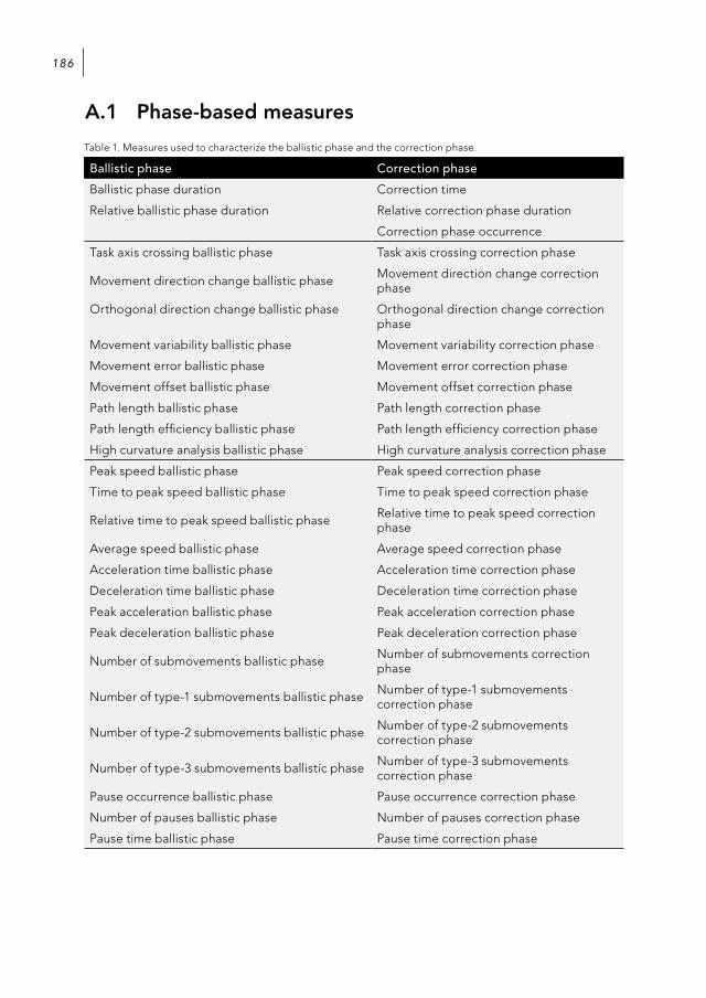
186
A.1 Phase-based measures
Table 1. Measures used to characterize the ballistic phase and the correction phase.
Ballistic phase Correction phase
Ballistic phase duration Correction time
Relative ballistic phase duration Relative correction phase duration
Correction phase occurrence
Task axis crossing ballistic phase Task axis crossing correction phase
Movement direction change ballistic phase Movement direction change correction phase
Orthogonal direction change ballistic phase Orthogonal direction change correction phase
Movement variability ballistic phase Movement variability correction phase
Movement error ballistic phase Movement error correction phase
Movement offset ballistic phase Movement offset correction phase
Path length ballistic phase Path length correction phase
Path length efficiency ballistic phase Path length efficiency correction phase
High curvature analysis ballistic phase High curvature analysis correction phase
Peak speed ballistic phase Peak speed correction phase
Time to peak speed ballistic phase Time to peak speed correction phase
Relative time to peak speed ballistic phase Relative time to peak speed correction phase
Average speed ballistic phase Average speed correction phase
Acceleration time ballistic phase Acceleration time correction phase
Deceleration time ballistic phase Deceleration time correction phase
Peak acceleration ballistic phase Peak acceleration correction phase
Peak deceleration ballistic phase Peak deceleration correction phase
Number of submovements ballistic phase Number of submovements correction phase
Number of type-1 submovements ballistic phase Number of type-1 submovements correction phase
Number of type-2 submovements ballistic phase Number of type-2 submovements correction phase
Number of type-3 submovements ballistic phase Number of type-3 submovements correction phase
Pause occurrence ballistic phase Pause occurrence correction phase
Number of pauses ballistic phase Number of pauses correction phase
Pause time ballistic phase Pause time correction phase

Appendices 187
A.2 Clustering selection taskTable 1. 1D patterns identified by recursive clustering analysis within the overall movement measures (T=movement time, E=error measures, PB=position-based measures, VB=velocity-based measures).
Overall (T, E, PB) Overall (T, E, PB, VB)
(a) (a)
(b) (b)
(c) (c)
(d)
(e)
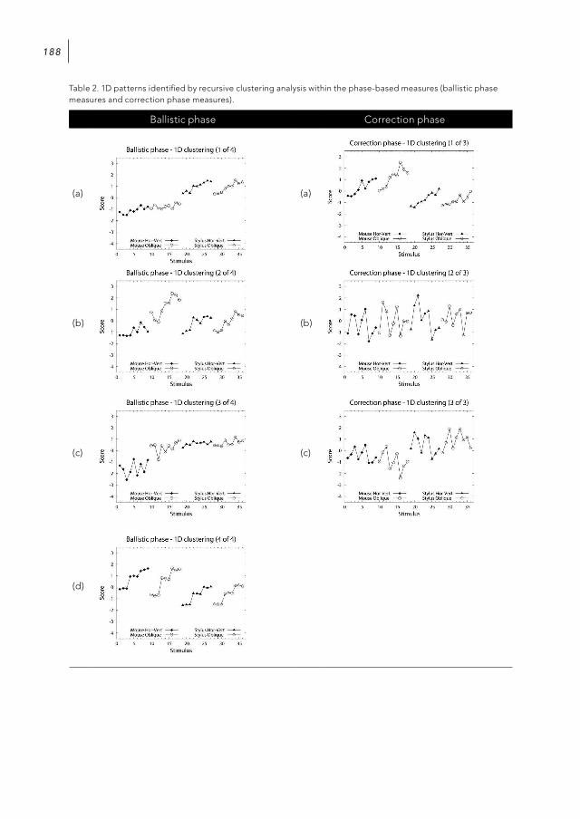
188
Table 2. 1D patterns identified by recursive clustering analysis within the phase-based measures (ballistic phase measures and correction phase measures).
Ballistic phase Correction phase
(a) (a)
(b) (b)
(c) (c)
(d)

Appendices 189
A.3 Clustering tracing taskTable 1. 1D patterns identified by recursive clustering analysis within the overall movement measures (T=movement time, E=error measures, PB=position-based measures, VB=velocity-based measures).
Overall (T, E, PB) Overall (T, E, PB, VB)
(a) (a)
(b) (b)
(c) (c)
(d)
(e)

190
Table 2. 1D patterns identified by recursive clustering analysis within the phase-based measures (ballistic phase measures and correction phase measures).
Ballistic phase Correction phase
(a) (a)
(b) (b)
(c) (c)
(d)
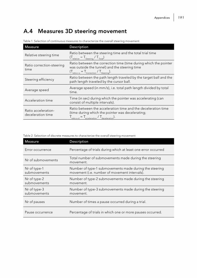
Appendices 191
A.4 Measures 3D steering movement
Table 1. Selection of continuous measures to characterize the overall steering movement.
Measure Description
Relative steering time Ratio between the steering time and the total trial time (Trelative = TSteering / TTotal)
Ratio correction- steering time
Ratio between the correction time (time during which the pointer was outside the tunnel) and the steering time (Tratio c-s = TCorrection / TSteering).
Steering efficiency Ratio between the path length traveled by the target ball and the path length traveled by the cursor ball.
Average speed Average speed (in mm/s), i.e. total path length divided by total time.
Acceleration time Time (in sec) during which the pointer was accelerating (can consist of multiple intervals).
Ratio acceleration-deceleration time
Ratio between the acceleration time and the deceleration time (time during which the pointer was decelerating; Tratio a-d = Tacceleration / Tdeceleration).
Table 2. Selection of discrete measures to characterize the overall steering movement
Measure Description
Error occurrence Percentage of trials during which at least one error occurred
Nr of submovements Total number of submovements made during the steering movement.
Nr of type-1 submovements
Number of type-1 submovements made during the steering movement (i.e. number of movement intervals).
Nr of type-2 submovements
Number of type-2 submovements made during the steering movement.
Nr of type-3 submovements
Number of type-3 submovements made during the steering movement.
Nr of pauses Number of times a pause occurred during a trial.
Pause occurrence Percentage of trials in which one or more pauses occurred.
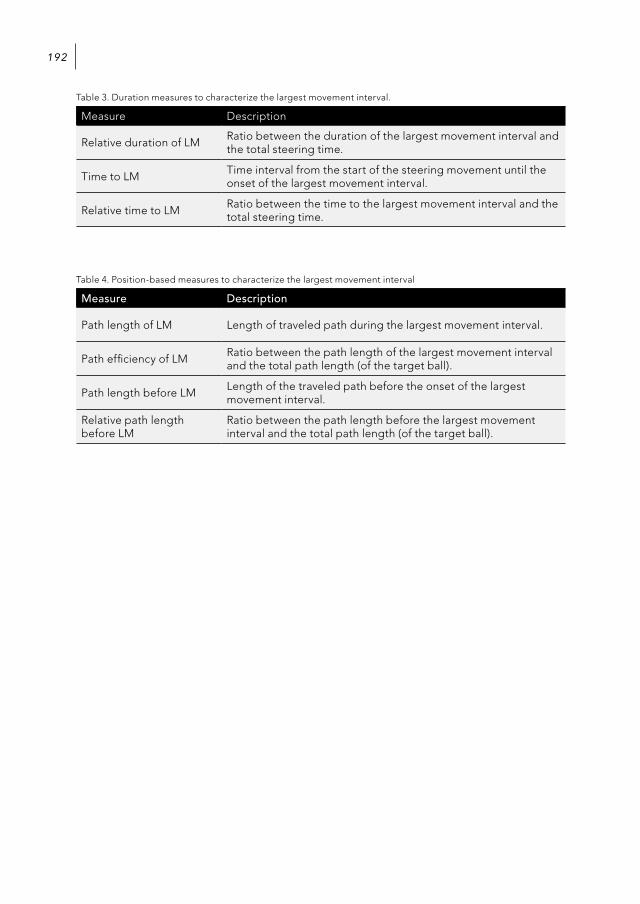
192
Table 3. Duration measures to characterize the largest movement interval.
Measure Description
Relative duration of LM Ratio between the duration of the largest movement interval and the total steering time.
Time to LM Time interval from the start of the steering movement until the onset of the largest movement interval.
Relative time to LM Ratio between the time to the largest movement interval and the total steering time.
Table 4. Position-based measures to characterize the largest movement interval
Measure Description
Path length of LM Length of traveled path during the largest movement interval.
Path efficiency of LM Ratio between the path length of the largest movement interval and the total path length (of the target ball).
Path length before LM Length of the traveled path before the onset of the largest movement interval.
Relative path length before LM
Ratio between the path length before the largest movement interval and the total path length (of the target ball).

Appendices 193
Table 5. Velocity-based measures to characterize the largest movement interval
Measure Description
Speed of LM Average speed (in mm/s), i.e. path length of largest movement interval divided by the duration of the largest movement interval.
Peak speed Maximum speed (in mm/s) reached during the largest movement interval.
Peak acceleration Maximum acceleration (in mm/s2) reached during the largest movement interval.
Peak deceleration Maximum deceleration (in mm/s2) reached during the largest movement interval.
Relative time to peak speed
Ratio between the time to peak speed (time interval from the onset of the largest movement interval to the moment the peak speed is reached) and the duration of the largest movement interval
Relative acceleration time of LM
Ratio between the time during which the pointer was accelerating during the largest movement interval and the duration of the largest movement interval.
Ratio acceleration-deceleration time of LM
Ratio between the acceleration time and the deceleration time of the largest movement interval (Tratio a-d = Tacceleration / Tdeceleration).
Density of nr of submovements
Ratio between the number of submovements and the path length of the largest movement interval.
Density of nr of type-2 submovements
Ratio between the number of type-2 submovements and the path length of the largest movement interval.
Density of nr of type-3 submovements
Ratio between the number of type-3 submovements and the path length of the largest movement interval.

194
Summary
For the development of 3D interactive systems, such as MR desktop systems, that are easy to use and learn it is important to systematically evaluate the various system components, such as input devices, interaction techniques and system parameters. However, most experimental studies in which (parts of) 3D interaction systems are evaluated apply tasks that have idiosyncratic characteristics of the available systems. Furthermore, these studies often apply only a limited number of performance metrics, such as time and error, to assess performance. Therefore, a more thorough method is developed for the quantitative evaluation of spatial input devices and interaction techniques. The main contributions of the thesis correspond to four distinct components of this quantitative approach towards the evaluation of interaction movements, of which the initial development is based on 2D interaction movements.
First, a more general model for Fitts’ law is proposed which allows for a more precise modeling of the relationship between movement time and task difficulty by i.a. incorporating Box-Cox functions. Results showed that especially in the case of a 2D tracing task a power-law function different from the originally proposed logarithmic function is required to accurately describe the relationship between movement time and task difficulty. Another advantage of this more advanced data modeling is that the entire distribution of the observed data is considered and not merely the average movement times. Results showed that non-linear transformations on the movement time distributions are able to resolve problems with the normality and homogeneity of variance, especially in the case of the 2D tracing task. Based on the optimized Fitts’ law modeling an alternative measure for throughput is proposed that takes into account the offset, gain and form of the relationship between movement time and task difficulty (i.e. performance rate). Both the

196
optimized modeling and the performance rate measure resulted in a higher contrast between experimental conditions.
Second, it is argued to not only apply movement time and error rate measures but also to use more complex measures such as position-based and velocity-based measures which require more effort with respect to data logging and computation. Although differences were expected between the evaluated 2D input devices (mouse and stylus), results showed that movement time was not able to reveal any differences in the case of the 2D selection and tracing tasks. The error rate was only able to reveal differences between the input devices in the case of the 2D tracing task. The inclusion of position-based measures and subsequently velocity-based measures in the recursive clustering analysis revealed additional patterns in the data of which some were able to discriminate well between the two input devices.
Third, a method is proposed that more intuitively divides movements into five movement phases: latency phase, initiation phase, ballistic phase, correction phase and verification phase. In contrast to the overall movement time, the duration of the ballistic, correction and verification phases and the occurrence of the latency, initiation, correction and verification phases were able to reveal differences between the evaluated input devices. The characterization of especially the ballistic phase and the correction phase, by means of position-based and velocity-based measures, resulted in a more detailed description of the 2D interaction movements. The recursive clustering analysis and the multi-directional scaling (MDS) analysis showed that some of the patterns revealed by the ballistic phase and the correction phase measures were complementary to the patterns revealed by the overall movement measures. In addition, certain position-based and velocity-based measures displayed a higher discriminative ability between the 2D input devices when

Summary 197
characterizing the ballistic and the correction phase than when characterizing the overall movement.
Finally, it is illustrated that recursive clustering analysis can be used to select measures in a more targeted way by identifying the 1D pattern that can best discriminate between the different levels of a certain independent variable. The performance measures that are able to reveal this selected 1D pattern can subsequently provide a clear description of the main aspects in which the interaction movements differ from each other with respect to this independent variable (e.g. the two input devices in the case of the 2D experiment).
Although the initial development of the quantitative evaluation method is based on 2D interaction movements, it is demonstrated that the different components of the evaluation method can also be used in usability tests evaluating 3D computer interactions. This means that the proposed methodology can be a valuable tool for designers and researchers of spatial input devices and interaction techniques to evaluate and further improve their design solutions.

198

Acknowledgements
“Strength does not come from physical capacity. It comes from an indomitable will.” (Mahatma Ghandi)
Over the past few years I’ve experienced that utmost determination is a necessity when pursuing a doctorate degree. Yet, I couldn’t have succeeded without the help of many others. First of all, I would like to thank my promotor and daily supervisor Jean-Bernard. I learned a great deal from our discussions and your vision on sound statistical modeling. At times you’ve shown me what the Dutch saying ‘vechten tegen de bierkaai’ entails in the scientific world and you taught me not to give up. Thank you Robert, for being my second promotor. I enjoyed our cooperation within the QUASID project together with your PhD students Ferdi and Lei. I would also like to thank the members of my PhD committee: Berry, David, Ravin and Wijnand. Your remarks and insightful feedback helped me to further improve this dissertation.
Dima and Miguel, thank you for your support and our frequent and inspiring Skype discussions. Maybe one day we will write that article. Also thanks to my former colleagues of the UCE group. It has been a true privilege to be a part of this research group. Without my colleagues in room 2.44 it wouldn’t have been as much fun. Thank you Abdullah, Aga, Alex, Berke, Derya, Evan, Iris, Javed, Javier, Maurits, Metaxas, Saskia, Swethan, Qonita and Wouter for all the coffee and lunch breaks we enjoyed together.

200
My gratitude also goes to my family and friends for keeping me mentally sane. Mum and dad, you’ve always been there for me when I needed you and that means the world to me. Especially, the last couple of months you’ve helped me tremendously by watching your granddaughter when I needed to work on this dissertation. Mieke, Ayalies and Marleen, thank you for encouraging me and for listening to me when I once again complained about the progress of this work. Now I have to find something else to complain about! I would also like to thank and compliment Saskia Renders for her hard work on the graphical design and the layout of this book.
Lauren, my precious little girl, you entered our world when I was almost at the finish line. It has been a challenge to take the final few steps with you depending on me, but we did it! I can honestly say: “How wonderful life is while you’re in the world” (Elton John). This also applies to Victor, the love of my life. ‘Lief’, you are truly the definition of support. Your patience and your relentless belief in me gave me the strength to carry this through to the end. I do not have words enough to express my gratitude. This book is dedicated to you.

Curriculum Vitae
Karin Nieuwenhuizen was born on December 3rd 1980 in Geldrop, the Netherlands. In 2004 she obtained her psychology degree at the Maastricht University (UM). She majored in cognitive ergonomics and graduated on the subject of designing auditory alarm signals for an Intensive Care Unit that were easy to learn and to identify. In 2004 she entered the postgraduate User System Interaction (USI) program to further specialize in user-centered design methodologies. She obtained her PDEng degree with the thesis entitled ‘Investigation of the Potential Halo Effect of HomeLab on User Evaluations’ in 2006. Subsequently, she started her PhD research within the QUASID (Quantitative Spatial Interaction Design) project at the User Centered Engineering group of the department of Industrial Design at the Eindhoven University of Technology (TU/e). The results of this research, focusing on the development of a quantitative method for the evaluation of spatial input devices and interaction techniques used especially in mixed-reality desktop systems, are presented in this dissertation. During the completion of this dissertation she was also employed as a usability researcher at a small commercial company.

202
List of publicationsNieuwenhuizen, K., & Martens, J.-B. (2014). Advanced Modeling of Selection and Steering Data: Beyond Fitts’ Law. Manuscript submitted for publication.
Nieuwenhuizen, K., Aliakseyeu, D., & Martens, J.-B. (2010). Insight into goal-directed movement strategies. In Proceedings of the SIGCHI Conference on Human Factors in Computing Systems (pp. 883–886). New York, NY, USA: ACM Press.
Nieuwenhuizen, K., Liu, L., van Liere, R., & Martens, J.-B. (2009). Insights from dividing 3D goal-directed movements into meaningful phases. IEEE Computer Graphics and Applications, 29(6), 44–53.
Nieuwenhuizen, K., Aliakseyeu, D., & Martens, J.-B. (2009). Insight into goal-directed movements: beyond Fitts’ law. In Proceedings of the IFIP International Conference on Human-Computer Interaction (pp. 274–287). Berlin, Heidelberg: Springer-Verlag.
Liu, L., van Liere, R., Nieuwenhuizen, C., & Martens, J.-B. (2009). Comparing aimed movements in the real world and in virtual reality. In Proceedings of the IEEE Conference on Virtual Reality (pp. 219–222). Washington, DC, USA: IEEE Computer Society.

QUANTITATIVE ANALYSIS OF COMPUTER INTERACTION
MOVEMENTS
Karin Nieuwenhuizen
QU
AN
TITATIV
E A
NA
LYSIS
OF C
OM
PU
TE
R IN
TE
RA
CT
ION
MO
VE
ME
NT
S KA
RIN
NIE
UW
EN
HU
IZE
N
ISBN: 978-90-386-3839-3ISBN: 978-90-386-3839-3
QUANTITATIVE ANALYSIS
OF COMPUTER INTERACTION MOVEMENTS
Op woensdag 13 mei 2015 om 16.00 uur vindt de
promotie plaats in zaal 4 van het Auditorium van
de TU/e.
Aansluitend is er een receptie waarvoor u van
harte bent uitgenodigd.
Karin Nieuwenhuizen
tot het bijwonen van de openbare
verdediging van mijn proefschrift
UITNODIGING