quantitative analysis of systems beyond markov …lcs.ios.ac.cn/~zhanglj/slides/buchholz.pdfls...

LS Informatik IV

Quantitative Analysis of Systems

– Beyond Markov Models -

Peter BuchholzInformatik IVTU Dortmund

Peter Buchholz: Beyond Markov Models 1

LS Informatik IV

Overview

1. Beyond Markov Automata

2. Analysis of an Automaton

3. Equivalence of Automata

4. Some Aspects of Model Checking

5. Conclusions


LS Informatik IV

A Stochastic Automata ModelAn SA is defined as (L, ini , C, ena, sus, trans, res) where

I L = {1, . . . ,N} is a finite set of locations (automata states),I ini : L → [0, 1] defines the initial distribution over the set of locationsI C is a finite set of clock processes with classes (defined later)

(K is the set of clock process class pairs),I ena : L → C enabled clock processes in a location,I sus : L → C suspended clock processes in a location, for I ∈ L,

ena(I ) ∩ sus(I ) = ∅,I trans : L×K×L → [0, 1] is the transition function that assigns to a

source location, an enabled clock process class pair and a destinationlocation a probability distribution over the set of locations,

I res : L ×K × L → C reset function.


LS Informatik IV

Example 1:

c1 c2

1

c1 c4

c2 c3

c3

c3

Queueing System with

service times)

(general inter−arrival and

c1

c3

c2

c4

c2

c3

c1

c3

preemptive pritoity resume

class 1 (blue) with priority

5

c4

2

3

4

c3 service 1

c4 service 2

c2 arrival 2

c1 arrival 1


LS Informatik IV

Example 2:

c1 c4 c5

c6

up

down

c2 c6

c1 c4 c5

c3 c6 c4

c5 c6

reboot failure maintenance

c4 maintenance (2 classes wait and duration)

c1 failure (2 classes, soft and hard)

c3 repair

c2 reboot

c6 shut down

c5 gain

c5 res(c6)

c1,k1 c1,k2 c4,k1

c6 c6 c6

c2

c3

c4,k2


LS Informatik IV

How to model clock processes?

I In principle every stochastic process may be used

I But we would like to analyze the process numerically/analytically!

I Use some form of phase type process

I Markov processes and beyond ...!?


LS Informatik IV

How to model clock processes?I In principle every stochastic process may be used

I But we would like to analyze the process numerically/analytically!

I Use some form of phase type process

I Markov processes and beyond ...!?


LS Informatik IV

Markov Automata (MA):I clock process c ∈ C is an MMAP:(

π(c)0 ,G(c)

0 ,G(c)1 , . . . ,G(c)

k

)nc is the size of the state space π(c)

0 is the initial vector

G(c)0 is the generator of an absorbing Markov process

G(c)k (1 ≤ k ≤ K ) are non-negative,

G(c)0 +

∑Kk=1 G(c)

k is an irreducible generator matrix

Probabilistic interpretation of the behavior


LS Informatik IV

Phase type processes beyond Markov processes:

Matrix-exponential (ME) distributions: (π0,G0) such that

F(π0,G0) = 1− π0eGot I1

is a valid distribution function.Example:

π0 = (2.63479,−1.22850,−0.406283)

G0 =

−2.25709 0 00 −2.25709 −2.3381870 2.338187 −2.25709

distribution with CV 2 = 0.2009


LS Informatik IV

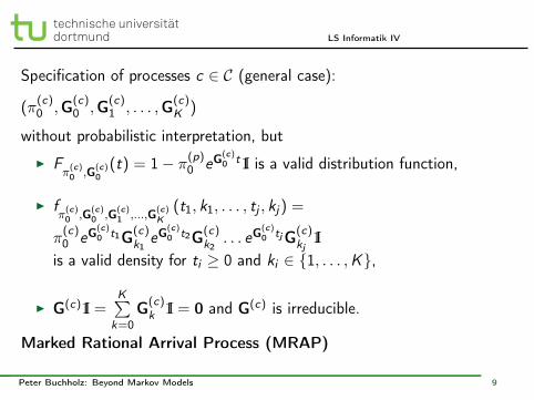
Specification of processes c ∈ C (general case):

(π(c)0 ,G(c)

0 ,G(c)1 , . . . ,G(c)

K )

without probabilistic interpretation, but

I Fπ

(c)0 ,G(c)

0(t) = 1− π(p)

0 eG(c)0 t I1 is a valid distribution function,

I fπ

(c)0 ,G(c)

0 ,G(c)1 ,...,G(c)

K(t1, k1, . . . , tj , kj) =

π(c)0 eG(c)

0 t1G(c)k1

eG(c)0 t2G(c)

k2. . . eG(c)

0 tjG(c)kj

I1is a valid density for ti ≥ 0 and ki ∈ {1, . . . ,K},

I G(c) I1 =K∑

k=0G(c)

k I1 = 0 and G(c) is irreducible.

Marked Rational Arrival Process (MRAP)


LS Informatik IV

Behavior of MRAPs:I process behaves deterministically according to the ODE π̇ = πG0

(i.e., πt = π0eG0t)

I at time t an event of type/class k occurs with density πtGk I1

I if event k occurs at time t, the state changes from πtπt I1 to πtGk

πtGk I1

state is given by the whole vector πt

Piecewise Deterministic Markov Process

Behavior is deterministic for a given historyH = (t0, k1, t1, k2, . . . , tH−1, kH , tH)(removing the stochastic part)Peter Buchholz: Beyond Markov Models 10

LS Informatik IV

Some properties of MRAP (π0,G0,G1, . . . ,GK ):

I the MRAP is class random if for every state π that is reached afteran arbitrary history H πeG0t′Gk holds for every k ∈ {1, . . . ,K} andsome t ′ ≥ 0

I the MRAP has an equivalent Markovian representation if anequivalent MMAP exists (definition of equivalence later)

I MRAPs without a finite MMAP representation exist

I the MRAP is minimal if no equivalent MRAP with a state space of asmaller dimension exists.


LS Informatik IV

Behavior of an SA (with MRAPs):

I the initial vector π0 =(π1

0, . . . , πN0)

where πI0 = νI ⊗p∈ena(I )∪sus(I ) π

(p)0 and νI is the probability to start

in location I

I in a location I MRAPs from ena(I ) behave deterministicallyaccording to the ODE π̇ = π ⊕c∈ena(I ) G(c)

0

I location changes occur according to events defined by the rates ofenabled MRAPs

I state changes occur at event times with respect toI state change in the MRAP that causes the eventI enabling/suspending/disabling of events in the destination locationI resetting of event due to function res(.)

An SA describes an MRAP!Peter Buchholz: Beyond Markov Models 12

LS Informatik IV

Analysis of an SA with representation (π0,G0,G1, . . . ,GK ):I expectation of the state at time t:

pt = E [πt ] = π0e(G0+∑K

k=1 Gk)t

I state at time t for history H = (t0, k1, t1, . . . , kH , tH) witht =

∑Hh=1 th:

πt =π0eGot0

∏Hh=1 Gkhe

G0th

π0eGot0∏H

h=1 GkheG0th I1

I if values of the state components in πt or pt are added, then aprobability distribution over the locations of the SA is defined


LS Informatik IV

Equivalence of SAs:1. Locations of the SA are observable

equivalent SAs have isomorphic locations but possibly differentprocesses in C

2. Locations observe predicatessets of locations with different predicates have to be distinguished,but not locations with the same predicates

3. Locations are not observablelocations need not be distinguished, only events are observable

1. and 2. can be transformed in 3. by defining pseudo events for statesthat have to be distinguished, e.g., event e is state I withtrans(I , e, I ) = 1 and corresponding process with G0 = (−µ), G1 = (µ).


LS Informatik IV

Equivalence of MRAPs

(π0,G0,G1, . . . ,GK ) and (φ0,H0,H1, . . . ,HK ) are equivalent

if and only if for all histories H = (t0, k1, t1, . . . , kH , 0):

π0

(H∏

h=1

eG0th−1Gkh

)I1 = φ0

(H∏

h=1

eH0th−1Hkh

)I1

i.e., the conditional density of observing a sequence of events is identicalfor both MRAPs


LS Informatik IV

Let (π0,G0,G1, . . . ,GK ) and (φ0,H0,H1, . . . ,HK ) be two equivalentMRAPs of size m and n (m ≥ n), respectively.

Then one of the following two relations hold:1. there exists a m × n matrix V with:

V I1 = I1, π0V = φ0 and GkV = VHk for all k = 0, . . . ,K

2. there exists an n ×m matrix W with:

W I1 = I1, π0 = Wφ0 and WGk = HkW for all k = 0, . . . ,K

V or W can be efficiently computed to find a minimal equivalentrepresentation for a given MRAP


LS Informatik IV

An Example:

π0 = (0.5, 0, 0, 0.5) , G0 =

−1 1 0 00 −2 2 00 0 −3 30 0 0 −4

,

G1 =

0 0 0 00 0 0 00 0 0 01.5 0 0 1.5

, G2 =

0 0 0 00 0 0 00 0 0 00.5 0 0 0.5

An equivalent MRAP of size 3

φ0 = (0, 0, 1) ,H0 =

−1.36364 4.13365 −6.65777−1.14992 −1.46376 4.02489

0 1.1726 −3.1726

,

H1 =

0 0 2.915820 0 −1.058410 0 1.5

,H2 =

0 0 0.971940 0 −0.35280 0 0.5

.


LS Informatik IV

Computation of minimal equivalentrepresentations

I compute minimal representations for all processes in C

I compute minimal representation for the whole SA

Steps for larger state spaces:

1. compute stochastic bisimulation (ordinary and inverse)

2. compute the minimal representation from the minimized processesaccording to bisimulation


LS Informatik IV

Model Checking of SAsCSL formulas for SAs

I tt is a location formula

I an atomic proposition a ∈ AP is a location formula

I if Φ and Ψ are location formulas, so are ¬Φ and Φ ∨Ψ,

I if Φ is a location formula, then so is Sonp,

I if ϕ is a path formula, the Ponp(ϕ) is a location formula,

I if Φ and Ψ are location formulas, then XintΦ and ΦUintΨ are pathformulas.

int ⊆ R≥0, on∈ {<,≤,≥, >} and p ∈ [0, 1]


LS Informatik IV

Model Checking Approaches:

I formulas with atomic propositions for locations are evaluated as usual

I steady state analysisI for irreducible SAs solve p

(∑Kk=0 Gk

)= 0 or

p(∑K

k=1 Gk

)(−G0)−1 = 0 subject to p I1 = 1

I otherwise determine the strongly connected components and computethe stationary vector for strongly connected components(locations may belong to more than one strongly connectedcomponent)

add the values in π belonging to locations to obtain a probabilitydistribution


LS Informatik IV

Model Checking Approaches:Compute probabilities for path formulas:

I for ΦU[t0,t1]Ψ (0 ≤ t0 ≤ t1):

I make all locations that do not observe Φ or Ψ absorbing and computeb1 = e

∑Kk=0 Gk [¬Φ∨¬Ψ](t1−t0) I1

I make all locations that do not observe Φ absorbing and computeb0 = e

∑Kk=0 Gk [¬Φ]t0b1

I for each I ∈ LProbI (ΦU[t0,t1Ψ) = ⊗p∈ena(I )∪sus(I )π

(p)0 · bI

0 orProbI (ΦU[t0,t1Ψ) = pI · bI

0for some vector p reached during an execution of the SA

I check ProbI (ΦU[t0,t1Ψ) on p


LS Informatik IV

Model Checking Approaches:

I for X[t0,t1]Φ (0 ≤ t0 ≤ t1) with initial vector ⊗p∈ena(I )∪sus(I )π(p)0 :

for each location I ∈ LI define

F(p)I ,Φ =

∑J∈{1,...,N},Φ(J)=tt

∑Kpk=1 trans(I , (p, k), J)G(p)

k and

F(p)I =

(G(p)

0 F(p)I ,Φ I1

0 0

)

compute(b(p)

I , β(p)I

)=(π

(p)0 eG(p)

0 t0 , 0)

eF(p)I (t1−t0)

I check∑

p∈ena(I ) β(p)I on p

I similar approach for initial vector pI


LS Informatik IV

Conclusions

I new class of automata

I interpretation as a piecewise deterministic Markov process

I numerical analysis

I equivalence relations

I first ideas for model checking state labels/rewards

I composition of SAs can be defined and preserves equivalence(not presented here)

I model checking path labels (not presented here)


LS Informatik IV

Open issues

I complete characterization of equivalent automata by CSL formulas

I introduction of indeterminism

I decision whether an automaton is valid SA(vector matrices describe a valid stochastic process)

I decision whether an SA has an equivalent representation as an MA


LS Informatik IV

Thank you!


quantitative analysis of systems beyond markov …lcs.ios.ac.cn/~zhanglj/slides/buchholz.pdfls...

Documents