Quantitative Finance II

Introduction to Mathematica: Simulation of Various Time Series

Summer Semester 2009/2010 by Jozef Baruník

* If viewed in .pdf format - for full functionality use Mathematica 7 notebook (.nb) version of this .pdf

This material serves as an general introduction to Mathematica environment including methods forTime Series simulation, Exporting and Importing the simulates Series, Plots, etc. as well as workwith Financial Data.

Introduction to Mathematica

Use Mathematica just like a calculator: you type in a question and Mathematica gives you theanswer Always use "Shift + Enter" to evaluate the input:

2 + 2

2

Type "2" "spacebar" and "2" to multiply:

2 µ 2

4

2D quick plot of function

Plot@Sin@1.5 xD^2, 8x, 0, 10<D

2 4 6 8 10

0.2

0.4

0.6

0.8

1.0

What is wrong? 2D quick plot does not work.Always use capital letters of functions, if anything goes "blue", it means that the funciton is unde-fined and Mathematica do not know what to do. To correct this line, just use capital P in "Plot":

plot@Sin@1.5 xD^2, 8x, 0, 10<D

plotASin@1.5 xD2, 8x, 0, 10<E

Go interactive and explore the behavior of function SinHa xL2 when changing parameter a:

Manipulate@Plot@Sin@a xD, 8x, 0, 10<D, 8a, 1, 10<D

a

2 4 6 8 10

-1.0

-0.5

0.5

1.0

Rotate 3D plots (just click and rotate the plot). Be carefull to separate "x" and "y" by space!

Plot3D@Sin@x yD, 8x, -3, 3<, 8y, -2, 2<D

Go interactive and explore the behavior of function SinHa x yL2 when changing parameter a:

Manipulate@Plot3D@Sin@a x yD, 8x, 0, 3<, 8y, 0, 3<D, 8a, 1, 4<D

a

Create List

2 QF_Intro_to_Mathematica.nb

Create List

Table@i, 8i, 1, 10<D

81, 2, 3, 4, 5, 6, 7, 8, 9, 10<

Create List with step size

Table@i, 8i, 1, 10, 2<D

81, 3, 5, 7, 9<

Plot elements from list

ListPlot@Table@i^2, 8i, 0, 10, 2<DD

1 2 3 4 5 6

20

40

60

80

100

Plot elements from list and join them

ListPlot@Table@i^2, 8i, 0, 10, 2<D, Joined Ø TrueD

1 2 3 4 5 6

20

40

60

80

100

Do not know how to change the plot? Use HELP (click on ">>" to get full help of function)

? Plot

Plot@ f , 8x, xmin, xmax<D generates a plot of f as a function of x from xmin to xmax.Plot@8 f1, f2, …<, 8x, xmin, xmax<D plots several functions fi.  à

Simulation of Time Series

Simulate Gaussian White Noise of length 100

QF_Intro_to_Mathematica.nb 3

RandomReal@NormalDistribution@0, 1D, 100D

8-0.686707, -0.218381, -1.16088, -0.37313, 0.0494906, -1.1003, 0.243749, 0.148945,0.227386, -0.962981, 0.393586, 0.670044, 0.672376, 0.335671, 1.13432, -0.0743773,0.320686, 0.676653, 2.00726, -0.862832, 0.533586, 0.0478635, -1.67511, 0.997238,0.754853, 2.20484, -0.570669, -0.584319, -0.761533, 0.413886, 1.44649, 0.250877,0.120462, -0.348304, -0.381419, -1.3334, 0.690217, -0.294642, -0.621348,-1.00763, 1.11646, 0.272846, -0.405526, -0.344932, -0.179411, -0.465833,2.03893, 0.936651, 1.64247, 0.680343, -0.433698, -0.318865, -0.355071, -0.960908,-0.993452, 0.551928, 0.0369989, -0.809543, -0.0182234, -0.692205, -1.60214,0.450587, 0.102433, 0.121183, 0.332172, -0.266114, -0.0888837, 1.24322, 1.17231,-0.877914, -1.11828, -1.46671, -1.25267, -0.883514, 1.65832, -1.26849, 0.252409,-0.217343, 1.35487, -0.699556, -0.675679, -0.318231, 0.958456, 0.488199,-1.11016, 1.66337, -1.27434, 0.723305, -1.70289, 0.281487, 0.569813, 0.865684,0.258749, -1.03529, -0.866935, -1.83263, 0.228277, 0.516266, -1.80196, -1.23769<

Now we want to plot the Gaussian White Noise of length 1000, so first we simulate it, save tovariable "GWhiteNoise" and then plot:

GWhiteNoise = RandomReal@NormalDistribution@0, 1D, 1000D;

Note that if you use ";", the cell evaluates but does not show result (in this case we only wnat togenerate the series into the variable

ListPlot@GWhiteNoiseD

200 400 600 800 1000

-3

-2

-1

1

2

3

Use Joined to get the time series plot

ListPlot@GWhiteNoise, Joined Ø TrueD

200 400 600 800 1000

-3

-2

-1

1

2

3

Use Options to enhance the plot

4 QF_Intro_to_Mathematica.nb

ListPlot@GWhiteNoise, Joined Ø True, Frame Ø True, PlotStyle Ø BlackD

0 200 400 600 800 1000

-3

-2

-1

0

1

2

3

Simulate AR(1) process:

rt = f0 +f1 rt-1 + et,

where 8et< is assumed to be a white noise et ~ NI0, s2M

First set f parameters

fi0 = 0.2;fi1 = 0.9;

Generate "ar1" variable as list containing Gaussian White Noise, and then simply iterativelly generateAR(1) process

ar1 = Table@RandomReal@NormalDistribution@0, 1DD, 8500<D;Do@ar1@@tDD = fi0 + fi1 ar1@@t - 1DD + RandomReal@NormalDistribution@0, 1DD;,

8t, 2, Length@ar1D<D;

No we have AR(1) saved in "ar1" variable so we can plot it:

ListPlot@ar1, Joined Ø True, Frame Ø True, PlotStyle Ø BlackD

0 100 200 300 400 500

-4

-2

0

2

4

6

8

Now generate ARH2L time series

rt = f0 +f1 rt-1 +f2 rt-2 + et,

where 8et< is assumed to be awhite noise et ~ NI0, s2M.

Again set f parameters first:

QF_Intro_to_Mathematica.nb 5

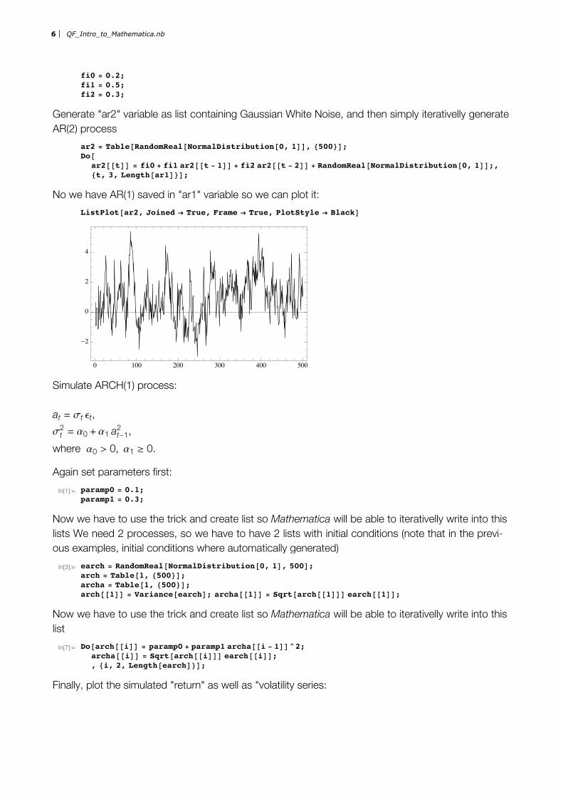
fi0 = 0.2;fi1 = 0.5;fi2 = 0.3;

Generate "ar2" variable as list containing Gaussian White Noise, and then simply iterativelly generateAR(2) process

ar2 = Table@RandomReal@NormalDistribution@0, 1DD, 8500<D;Do@

ar2@@tDD = fi0 + fi1 ar2@@t - 1DD + fi2 ar2@@t - 2DD + RandomReal@NormalDistribution@0, 1DD;,8t, 3, Length@ar1D<D;

No we have AR(1) saved in "ar1" variable so we can plot it:

ListPlot@ar2, Joined Ø True, Frame Ø True, PlotStyle Ø BlackD

0 100 200 300 400 500

-2

0

2

4

Simulate ARCH(1) process:

at = st et,

st2 = a0 +a1 at-1

2 ,

where a0 > 0, a1 ¥ 0.

Again set parameters first:

In[1]:= paramp0 = 0.1;paramp1 = 0.3;

Now we have to use the trick and create list so Mathematica will be able to iterativelly write into thislists We need 2 processes, so we have to have 2 lists with initial conditions (note that in the previ-ous examples, initial conditions where automatically generated)

In[3]:= earch = RandomReal@NormalDistribution@0, 1D, 500D;arch = Table@1, 8500<D;archa = Table@1, 8500<D;arch@@1DD = Variance@earchD; archa@@1DD = Sqrt@arch@@1DDD earch@@1DD;

Now we have to use the trick and create list so Mathematica will be able to iterativelly write into thislist

In[7]:= Do@arch@@iDD = paramp0 + paramp1 archa@@i - 1DD^2;archa@@iDD = Sqrt@arch@@iDDD earch@@iDD;, 8i, 2, Length@earchD<D;

Finally, plot the simulated "return" as well as "volatility series:

6 QF_Intro_to_Mathematica.nb

In[8]:= ListPlot@arch, Joined Ø True, Frame Ø True, PlotStyle Ø BlackDListPlot@archa, Joined Ø True, Frame Ø True, PlotStyle Ø BlackD

Out[8]=

0 100 200 300 400 5000.10

0.15

0.20

0.25

Out[9]=

0 100 200 300 400 500

-1.0

-0.5

0.0

0.5

1.0

1.5

Exportinh and Importing simulated Time Series and Figures

Export figure of simulated volatility to .pdf (eventually to any other format supported by Mathematica)

In[10]:= myfigure = ListPlot@arch, Joined Ø True, Frame Ø True, PlotStyle Ø BlackD;Export@"SimulatedVolatility.pdf", myfigureD

Out[11]= SimulatedVolatility.pdf

Export simulated ARCH series to .txt (eventually to any other format supported by Mathematica) soyou can use it by any other program

In[12]:= Export@"ARCHsimulatedseries.txt", archaD

Out[12]= ARCHsimulatedseries.txt

Exported time series and figures always goes to your home directory. To find out the home direc-tory, use :

In[13]:= Directory@D

You can also Import any data to Mathematica worksheet and work with it using Import:

In[17]:= importedseries = Import@"ARCHsimulatedseries.txt", "List"D;

And now plot imported series

QF_Intro_to_Mathematica.nb 7

Working with financial data in Mathematica

Mathematica has built in connection to lates financial databases. Internet connection and rightproxy settings needed for functioning.

Plot the stock market index S&P 500 evolution since January 1, 1987 :

In[21]:= DateListPlot@FinancialData@"SP500", "Jan. 1, 1987"D, Joined Ø TrueD

Out[21]=

1990 1995 2000 2005 2010200

400

600

800

1000

1200

1400

Plot the trading volume for GE stock from the beginning of 2007 until March 2010

In[25]:= DateListPlot@FinancialData@"GE", "Volume", 882007, 1, 1<, 82010, 3, 1<<D, Filling Ø AxisD

Out[25]=

Find the current exchange rate between euros and U.S. dollars:

In[26]:= FinancialData@"EURêUSD"D

Out[26]= 1.3633

Find the price of gold in U.S. dollars:

In[27]:= FinancialData@"XAUêUSD"D

Out[27]= 1123.5

8 QF_Intro_to_Mathematica.nb