quantitative methods and detection techniques in

Clemson UniversityTigerPrints

All Dissertations Dissertations

8-2007

QUANTITATIVE METHODS ANDDETECTION TECHNIQUES INHYPERSPECTRAL IMAGING INVOLVINGMEDICAL AND OTHER APPLICATIONSAnkita RoyClemson University, [email protected]

Follow this and additional works at: https://tigerprints.clemson.edu/all_dissertations

Part of the Optics Commons

This Dissertation is brought to you for free and open access by the Dissertations at TigerPrints. It has been accepted for inclusion in All Dissertations byan authorized administrator of TigerPrints. For more information, please contact [email protected].

Recommended CitationRoy, Ankita, "QUANTITATIVE METHODS AND DETECTION TECHNIQUES IN HYPERSPECTRAL IMAGINGINVOLVING MEDICAL AND OTHER APPLICATIONS" (2007). All Dissertations. 108.https://tigerprints.clemson.edu/all_dissertations/108

https://tigerprints.clemson.edu?utm_source=tigerprints.clemson.edu%2Fall_dissertations%2F108&utm_medium=PDF&utm_campaign=PDFCoverPages

https://tigerprints.clemson.edu/all_dissertations?utm_source=tigerprints.clemson.edu%2Fall_dissertations%2F108&utm_medium=PDF&utm_campaign=PDFCoverPages

https://tigerprints.clemson.edu/dissertations?utm_source=tigerprints.clemson.edu%2Fall_dissertations%2F108&utm_medium=PDF&utm_campaign=PDFCoverPages

https://tigerprints.clemson.edu/all_dissertations?utm_source=tigerprints.clemson.edu%2Fall_dissertations%2F108&utm_medium=PDF&utm_campaign=PDFCoverPages

http://network.bepress.com/hgg/discipline/204?utm_source=tigerprints.clemson.edu%2Fall_dissertations%2F108&utm_medium=PDF&utm_campaign=PDFCoverPages

https://tigerprints.clemson.edu/all_dissertations/108?utm_source=tigerprints.clemson.edu%2Fall_dissertations%2F108&utm_medium=PDF&utm_campaign=PDFCoverPages

mailto:[email protected]

QUANTITATIVE METHODS AND DETECTION TECHNIQUES IN HYPERSPECTRAL IMAGING INVOLVING MEDICAL AND OTHER

APPLICATIONS

A Dissertation Presented to

the Graduate School of Clemson University

In Partial Fulfillment of the Requirements for the Degree

Doctor of Philosophy Physics

by Ankita Roy August 2007

Accepted by: Dr. Bruce Rafert, Committee Chair

Dr. John Ballato Dr. Joseph R. Manson

Dr. Emil Alexov

- ii - ii

ABSTRACT

This research using Hyperspectral imaging involves recognizing targets through spatial

and spectral matching and spectral un-mixing of data ranging from remote sensing to

medical imaging kernels for clinical studies based on Hyperspectral data-sets generated

using the VFTHSI [Visible Fourier Transform Hyperspectral Imager], whose high

resolution Si detector makes the analysis achievable. The research may be broadly

classified into (I) A Physically Motivated Correlation Formalism (PMCF), which places

both spatial and spectral data on an equivalent mathematical footing in the context of a

specific Kernel and (II) An application in RF plasma specie detection during carbon

nanotube growing process. (III) Hyperspectral analysis for assessing density and

distribution of retinopathies like age related macular degeneration (ARMD) and error

estimation enabling the early recognition of ARMD, which is treated as an ill-conditioned

inverse imaging problem. The broad statistical scopes of this research are two fold- target

recognition problems and spectral unmixing problems. All processes involve

experimental and computational analysis of Hyperspectral data sets is presented, which is

based on the principle of a Sagnac Interferometer, calibrated to obtain high SNR levels.

PMCF computes spectral/spatial/cross moments and answers the question of how

optimally the entire hypercube should be sampled and finds how many spatial-spectral

pixels are required precisely for a particular target recognition. Spectral analysis of RF

plasma radicals, typically Methane plasma and Argon plasma using VFTHSI has enabled

better process monitoring during growth of vertically aligned multi-walled carbon

- iii - iii

nanotubes by instant registration of the chemical composition or density changes

temporally, which is key since a significant correlation can be found between plasma

state and structural properties.

A vital focus of this dissertation is towards medical Hyperspectral imaging applied to

retinopathies like age related macular degeneration targets taken with a Fundus imager,

which is akin to the VFTHSI. Detection of the constituent components in the diseased

hyper-pigmentation area is also computed. The target or reflectance matrix is treated as a

highly ill-conditioned spectral un-mixing problem, to which methodologies like inverse

techniques, principal component analysis (PCA) and receiver operating curves (ROC) for

precise spectral recognition of infected area.

The region containing ARMD was easily distinguishable from the spectral mesh plots

over the entire band-pass area. Once the location was detected the PMCF coefficients

were calculated by cross correlating a target of normal oxygenated retina with the de-

oxygenated one. The ROCs generated using PMCF shows 30% higher detection

probability with improved accuracy than ROCs based on Spectral Angle Mapper (SAM).

By spectral unmixing methods, the important endmembers/carotenoids of the MD

pigment were found to be Xanthophyl and lutein, while β-carotene which showed a

negative correlation in the unconstrained inverse problem is a supplement given to

ARMD patients to prevent the disease and does not occur in the eye. Literature also

shows degeneration of meso-zeaxanthin. Ophthalmologists may assert the presence of

- iv - iv

ARMD and commence the diagnosis process if the Xanthophyl pigment have

degenerated 89.9%, while the lutein has decayed almost 80%, as found deduced

computationally. This piece of current research takes it to the next level of precise

investigation in the continuing process of improved clinical findings by correlating the

microanatomy of the diseased fovea and shows promise of an early detection of this

disease.

- v - v

DEDICATION

I would like to dedicate this dissertation to my father, Arun Roy, who can only

experience this from his heavenly abode. He always wished me of achieving something

worthwhile during my teenage years, which inspired me to take up a doctoral program in

Physics later and complete my research voyage. I would also like to dedicate it to my

mother, Surabhi Roy, who is an amazing lady and whose continuous encouragement,

sacrifices and long lasting dream of me attaining the highest academic degree has

constantly motivated me to fulfill her long cherished dream. I will remain grateful to my

parents for their struggle to make me what I am today.

I met someone during my undergraduate years at the Indian Institute of Technology, who

later became my closest friend and constant motivator – my husband, Dr. Saswata Ghosh,

who was completing his doctoral studies along with me. I thank him for his patience,

suggestions, inspiration and understanding during these five long years and would like to

dedicate this dissertation to him along with my parents.

- vi - vi

ACKNOWLEDGEMENTS

First of all, I would like to acknowledge my advisor, Prof. Bruce Rafert, whose excellent

guidance in spite of his busy schedule of serving as the Graduate School Dean of

Clemson University and former Graduate School Dean of Michigan Tech, made this

research possible. At MTU, he initiated me to this research topic of hyperspectral

imaging science and helped me tremendously through our discussions and lab work to

accomplish the research objectives in attaining a doctorate in Physics from Clemson

University. I am extremely thankful to him for his continuous support through this long

journey from Houghton, MI to Clemson SC. I express my gratitude to him for always

believing in me and all the appreciation, which has boosted my confidence largely. I also

admire his incredible efforts in keeping the dissertation on track along with his

remarkable multi-tasking techniques, challenging me to set and exceed goals. I have

learnt a lot from him, which will benefit me a lot in the future years ahead.

I am grateful for the guidance of my dissertation committee: Dr. Joseph Manson, Dr.

John Ballato and Dr. Emil Alexov. The research meetings with them yielded valuable

insight for some of the investigations pursued in this dissertation.

I would like to thank Gene Butler and Kamel Belkacem-Boussaid of Kestrel Corp,

Albuquerque, NM for providing hyperspectral data-sets taken with the Fundus imager,

which were key data in the investigations of age-related macular degeneration using

hyperspectral imaging. I am thankful to Prof. Peter Barnes, Physics Department Chair at

- vii - vii

Clemson University for his support, Prof. Jacek Borysow, co-advisor for Masters Thesis

(related to doctoral dissertation) for his help in the Hyperspectral imaging research

application in Nanotechnology, Prof. Ravi Pandey, Chair of Physics Department at MTU

for his help during university transfer.

- viii - viii

TABLE OF CONTENTS

TITLE PAGE ............................................................................................................................................. i ABSTRACT .............................................................................................................................................. ii DEDICATION .......................................................................................................................................... v ACKNOWLEDGEMENTS .................................................................................................................... vi LIST OF TABLES .................................................................................................................................. xii LIST OF FIGURES ........................................................................................................................... …xiii CHAPTER

1 INTRODUCTION............................................................................................................................... 1

1.1 INTRODUCTION & MOTIVATION ................................................................................................... 1

1.2 THE TECHNOLOGY OF HYPERSPECTRAL IMAGING ....................................................................... 3

1.3 ADVANTAGES OF HYPERSPECTRAL IMAGING FOR CURRENT RESEARCH WITH VFTHSI .............. 9

2 INSTRUMENTATION, THEORY AND EXPERIMENTS ......................................................... 12

2.1 OVERVIEW OF THE VFTHSI ....................................................................................................... 12

2.2 THEORY AND DESIGN OF OPTICS IN IMAGER .............................................................................. 16

2.2.1 Physics of Temporal Coherence ........................................................................................... 17

2.2.2 The Sagnac Interferometer ................................................................................................... 18

2.2.3 Fourier Spectroscopy ............................................................................................................ 20

2.2.3.1 Mathematical derivation and importance of the autocorrelation function ................... 24

2.2.4 Fourier Transform Lens ........................................................................................................ 28

2.2.4.1 Theory of Quantitative FT Analysis ............................................................................ 32

2.2.4.2 Nyquist Frequency and sampling theorem .................................................................. 33

2.2.5 Cylindrical Lens ................................................................................................................... 35

2.2.6 Silicon Detector .................................................................................................................... 36

2.2.6.1 The Detector Array Design ......................................................................................... 37

- ix - ix

2.3 CALIBRATION OF THE SI DETECTOR: .......................................................................................... 39

2.4 GENERATING HYPERCUBES - ANALYSIS AND EXAMPLES ............................................................ 45

2.4.1 Experiments, Methods & Results ......................................................................................... 45

2.4.2 Noise Reduction, SNR, & Filtering ...................................................................................... 47

2.4.3 Generating the final Hypercube ............................................................................................ 49

3 PHYSICALLY MOTIVATED CORRELATION FORMALISM (PMCF) ................................ 52

3.1 METHODOLOGY ......................................................................................................................... 52

3.1.1 Correlation Moments ............................................................................................................ 55

3.2 CORRELATION RESULTS ............................................................................................................. 56

3.2.1 PMCF using MTU images (Spectral Matching) ................................................................... 58

3.2.2 Spatial matching with PMCF ................................................................................................ 63

3.3 CONCLUSIONS ............................................................................................................................ 66

4 APPLICATION OF HYPERSPECTRAL IMAGING IN RF PLASMA SPECIE DETECTION

DURING NANO-TUBE GROWING PROCESS .................................................................................... 68

4.1 EXPERIMENTAL DETAILS ........................................................................................................... 68

4.2 THE R-F DUAL PLASMA SOURCE DESCRIPTION ......................................................................... 70

4.3 CALIBRATION USING RF ARGON PLASMA .................................................................................. 74

4.4 RESULTS OF HYPERSPECTRAL ANALYSIS OF RF CH4 PLASMA .................................................. 82

4.5 PLASMA ANALYSIS CONCLUSIONS ............................................................................................. 88

5 ERROR ESTIMATION IN AN ILL-CONDITIONED INVERSE IMAGING PROBLEM OF

REFLECTANCE ........................................................................................................................................ 90

5.1 AGE RELATED MACULAR DEGENERATION [ARMD] ................................................................... 91

5.2 THE FUNDUS HYPERSPECTRAL IMAGING INSTRUMENT .............................................................. 94

5.2.1 Construction Details ............................................................................................................. 94

5.2.2 Details of the operational settings of the Fundus .................................................................. 99

- x - x

5.2.3 Data Collection & Processing ..............................................................................................100

5.3 IMPORTANCE & MOTIVATION OF RETINAL HSI ........................................................................106

5.4 MATHEMATICAL MODELS INVOLVING INVERSE IMAGING METHODS ........................................108

5.4.1 SVD with Generalized Inverse Methods .............................................................................111

5.4.2 Filtering Techniques ............................................................................................................114

5.4.3 Error Estimation ..................................................................................................................115

5.5 PRINCIPAL COMPONENT ANALYSIS TECHNIQUES ......................................................................117

5.6 DETECTION TECHNIQUES USING RECEIVER OPERATING CURVES ..............................................120

6 HYPER-SPECTRAL ANALYSIS & UN-MIXING OF MACULAR DEGENERATION

PIGMENT ..................................................................................................................................................124

6.1 INTRODUCTION..........................................................................................................................124

6.2 SPECTRAL ANALYSIS OF REFLECTANCE DATA ..........................................................................127

6.2.1 Spectral Analysis of Normal Oxygenated Retina ................................................................127

6.2.2 Analysis for the Macular Degeneration spectral Profile ......................................................133

6.2.2.1 Macular Degeneration Detection with PMCF for Subject ‘A’ ...................................138

6.2.2.2 Detection Techniques using Receiver Operating Curves for subject ‘A’ ...................142

6.2.2.3 PMCF Detection of MD for Subject ‘B’ ....................................................................146

6.2.2.4 Plotting spectra of Macular Degeneration from different parts of the interferogram .148

6.2.2.5 ROC detection for subject ‘B’ ....................................................................................151

6.2.2.6 ROC for subject ‘B’ based on Spectral Angle Mapper ..............................................153

6.3 LINEAR SPECTRAL UNMIXING PROBLEM OF MD USING INVERSE TECHNIQUES ........................158

6.3.1 Reconstruction of spectral profiles of different end-members of macular pigmentation from

reference literature .............................................................................................................................160

6.3.2 Results and Discussions for the Spectral Unmixing of MD ................................................169

7 CONCLUSIONS ..............................................................................................................................173

7.1 DISSERTATION SUMMARY .........................................................................................................173

- xi - xi

7.2 CONCLUSIONS FROM HYPER-SPECTRAL ANALYSIS & PHYSICALLY MOTIVATED CORRELATION

FORMALISM .............................................................................................................................................175

7.3 CONCLUSIONS ON APPLICATIONS ON MEDICAL HYPER-SPECTRAL IMAGING OF DISEASED RETINA

176

7.4 FUTURE RESEARCH DIRECTIONS ...............................................................................................179

7.4.1 Future work involving retinal hyper-spectral imaging ........................................................179

7.4.2 Future Work using PMCF ...................................................................................................181

APPENDIX………………………………………………………………………………………………..185

BIBLIOGRAPHY .....................................................................................................................................194

- xii - xii

LIST OF TABLES

Table 2.1. Ar –I Spectral lines observed with VFTHSI ............................................................................... 44

Table 4.1. RF Methane Plasma Spectral Lines. ............................................................................................ 74

Table 4.2. RF Argon plasma lines ................................................................................................................ 80

Table 5.1. Estimated Errors with no filters, TSVD, Tikhonov for ill-conditioned Reflectance Matrices. .116

Table 6.1. Table showing the Hg–I lines from NIST reference tables and their relative intensity values...130

Table 6.2. Spectral Information of Endmembers of MD .............................................................................161

Table 6.3. Percentage Compositions of MD components from Inverse Methods. ......................................169

Table 6.4. Statistics......................................................................................................................................170

Table 6.5. Primary Components. .................................................................................................................171

- xiii - xiii

LIST OF FIGURES

Figure1.1: HYPERCUBE SHOWING x,y, λ profiles IMAGE STACK……………………………. 7

Figure1.2: MD Hypercube ………………………………...……………………………………….…7

Figure 1.3: Diagram depicting Linear Un-Mixing problem and end-member analysis …………..….7

Figure 2.1a: Schematic of the VFTHSI ………………………………………………………..……12

Figure 2.1b: Visible Hyperspectral Imager ………………………………………………………….13

Figure 2.1c Actual set-up inside the interferometer …………………………………........................13

Figure 2.2.2a: Schematic of a Sagnac Interferometer………………………………………….…….18

Figure 2.2.1b: Intensity on the detector Vs normalized mirror displacement ………………….……21

Figure 2.2.2a: Schematic of a Fourier Transform lens ……………………………………………...27

Figure 2.2.4.2 Shannon Sampling Theorem Depiction ……………………………………….……..30

Figure 2.3a Showing Spectral Responsivity function of the detector………………………………...36

Fig 2.3b: Calibration Graph with He & Detector response data ………………………………..…....38

Fig2.3c RF Argon plasma Spectral Analysis ………………………………………………….……..39

Figure 2.4a: 2-D Image Interferogram & Filtered Signal Interferogram plot a row of the target …..40

Figure:2.4b: Signal and spectrum & Spatial Profile - He-Ne…………………………. ………….....41

Figure 2.4 c: Parametric Study of SNR Vs Resolution …………………………………………..….43

Figure 2.4d Spectrum hypercube for 1024 rows Vs frequency ……………………………………...45

Figure 2.4 e :Hypercubes of two different aerial targets ………………………………………..…...46

Figure 3.1: hypercube with x,y, λ profiles ……………………………………………………..…. ..50

Fig 3.2a Spectral-spectral Correlation of He-Ne target. ………………………………………..……52

Fig 3.2 b: Spatial-spatial correlation of He-Ne source. …………………………………………..…53

Fig 3.2c Spectral Library plots in ENVI of water, sky, buildings & greenery ……..…………..……54

Fig 3.2d: Cross Correlation Graph …………………………………………..………………..……...55

Fig 3.2e: Selected AOI within MTU Hypercube…………………..………………………………....55

- xiv - xiv

Fig 3.2f Correlation mesh-plots of all arrays in the AOI and a water pixel ……..………...……56

Fig 3.2g: 3-D histogram showing the Maximum value of correlation….…………………….…57

Fig 3.2h : AOI for spatial mapping with PMCF…………….…………………………………...58

Fig 3.2i: PMCF coefficient Vs Col Location for spatial mapping…….…………………………59

Fig 3.2j: Spatial mapping with PMCF……………………………….…………………………..60

Fig 4.2a : PE-CVD chamber (showing top and bottom plasma around electrodes) ………….…66

Figure 4.2b: Experimental setup of the dual RF-PECVD chamber…………………..……….…66

FIGURE 4.3a Spectral response function of the detector…………………………..…………....68

Fig 4.3b(i) He spectra with VFTHSI…………………………………………..………………...70

Fig 4.3b(ii): Pixel -Wavelength mapping…………………………………….………………....71

Fig 4.3c Interferogram of RF Argon Plasma in PECVD chamber………………………………72

Figure 4.3d: RF Argon plasma analysis…………………………………………………………73

Figure 4.4a: Plot of Two Rows of Signal Interferograms of the CH4 glow plasma…………….75

Figure 4.4b: The Interferogram Image of Methane Plasma……………………………………..75

Fig 4.4c: Interferogram of a frame during scanning of CH4 RF-plasma………………………...76

Figure 4.4d: Hyperspectral Analysis of Methane RF-Plasma Spectra…………………………..78

Figure 4.4e: SEM image of grown VA-MWCNTs……………………………………………..79

Fig 5.1: Diseased Retina showing growth of macular degeneration pigment…………….….…..84

Fig 5.2i The Schematic of Fundus Hyperspectral Imager…………………………………..…...85

Fig 5.2ii: A ray trace layout of the Fundus………………………………………………..……..86

Fig 5.2iii: Hyperspectral Fundus Imaging System …………………………………..……....…88

Fig 5.2iv: Hypercube of normal retina………………………………………………….….….…88

Fig 5.2v: Basic FTVHSI Processing……………………………………………………..….…...94

Fig 5.4: The spectra of 10 elements (unconvoluted/non-overlapped, well conditioned matrix)....98

Fig 5.5a : Simulated spectra-Xanthophyl pigment………………………………………….…....98

Fig 5.5b: Xanthophyl spectra from reference……………………………………….……….…..98

Figure 5.6 : TSVD filter……………………………………………………………….…….….101

- xv - xv

Figure5.7 : Tikhonov Filtering……………………………………………………………..101

Fig 5.8: Demonstration of ROCs……………………………………………….………….107

Fig6.2.1a : Image of Retina of a normal subject…………………………………..……….112

Fig6.2.1b (Left) shows the interferogram of normal retina…………………………..…….113

Figure 6.2.1c Filtered signal interferogram and the corresponding spectrum of a normal

retina (row 196)…………………………………………………………………….……..115

Fig 6.2.2a : Interferogram and scene – subject A………………………………….………117

Fig 6.2.2b Interferogram showing Hg emssion……………………………………….…...118

Fig 6.2.2c Calibration spectra- Hg emission spectra………………………………….…..119

Fig 6.2.2d interferograms and scene images of macular degeneration-subject ‘b’……..…120

Fig 6.2.2e interferograms and scene images of macular degeneration-subject ‘c’……..…121

Fig 6.2.2f: Correlation coefficient plot showing MD infected area –sub ‘A’…………..…122

Fig 6.2.2g: Mesh plot of all spectral profiles in the infected retina- subject ‘A’…………..124

Fig 6.2.2h: PMCF coefficients showing MD……………………………………….…..…125

Fig 6.2.2i: Histogram plots for detection probability and false alarm……………….….....127

Fig 6.2.2j: ROC analysis for subject ‘A’ diagnosed with macular degeneration…….….....128

Fig 6.2.2k: Correlation coefficient plot showing MD for subject ‘B’……………..…...….129

Fig 6.2.2l: Mesh plot of all spectral profiles in the infected retina –sub ‘B’………....……130

Fig 6.2.2 m: Macular Degeneration Pigment spectra at different parts of AOI……………131

Fig 6.2.2 n: MD Spectrum – known spectral library in the inverse problem………………132

Fig 6.2.2 o: error-bar plot of PMCF coefficients showing MD……………………...…….133

Fig 6.2.2p: Histogram plot of prob detection and false alarm – sub ‘B’…………………..134

Fig 6.2.2q: ROC graph for MD detection – Sub ‘B’……………………………………….135

Fig 6.2.2r : Schematic for Spectral Angle Mapper…………………………………...……137

Fig 6.2.2s: Plot of SAM coefficient in detecting MD cells for Subject ‘B’……………….138

Fig 6.2.2t: Histogram plot of pro detection and false alarm using SAM ………………….139

Fig 6.2.2u: ROC graph using SAM for sub ‘B’……………………………………………140

- xvi - xvi

Fig 6.3a: Xanthophyl spectrum……………………………………………………….145

Fig 6.3b: Lutein absorbance spectra…………………………………………………..146

Fig 6.3c: UV-VIS spectra of some carotenoids……………………………………….146

Fig 6.3d: Lutein Reflectance Spectrum……………………………………………….148

Fig 6.3e: Xanthophyl pigment reflectance spectrum………………………………….148

Fig 6.3f: Beta carotenoid Reflectance spectrum………………………………………149

- 1 - 1

Chapter 1

1 INTRODUCTION

1.1 Introduction & Motivation

Hyperspectral Imaging (HSI) is a powerful imaging tool for pattern recognition and

spectral analysis. The motivation of the research is recognizing targets through spatial

and spectral matching ranging from remote sensing targets to medical imaging kernels for

clinical studies. The thesis develops a set of new statistical models and quantitative

methods for detection techniques. Some of the models developed are aimed at

minimizing the error expressed in terms of its variance so that the constituent

composition of the target to be recognized can be estimated with reasonably high

precision, correlation moment model for hypercube sampling, spectral un-mixing models

for ill-conditioned data-sets and inverse imaging techniques. These models are robust in

nature and can be utilized to exploit any kind of data set like plasma images taken during

Carbon nanotube (CNT) growth to medical image matrices or even financial data-sets.

This research is based on Hyperspectral data-sets generated using the VFTHSI [Visible

Fourier Transform Hyperspectral Imager][15], whose extremely high resolution detector

makes the analysis achievable and can be broadly classified into (I) A Physically

Motivated Correlation Formalism (PMCF), which places both spatial and spectral data on

an equivalent mathematical footing in the context of a specific Kernel and (II) An

- 2 - 2

application in RF plasma specie detection during carbon nanotube growing process. (III)

Error estimation enabling the early detection of macular degeneration in a diseased retina,

which is treated as an ill-conditioned inverse imaging problem.

In PMCF, optimal combinations of independent data can be selected from the entire

Hypercube via the method of ‘Correlation Moments’ [5]. An experimental and

computational analysis of Hyperspectral data sets is presented in the next chapter, which

is based on the principle of a Sagnac Interferometer, calibrated to SNR [signal to noise

ratio] levels greater than 100. The captured Signal Interferograms of different remote

sensing targets and lab-based data with the provision of customized scan of targets with

the same exposures are processed using inverse imaging transformations and filtering

techniques to obtain the spectral profiles and generate Hypercubes to compute

Spectral/Spatial/Cross Moments. PMCF answers the question of how optimally the entire

hypercube should be sampled and finds how many spatial-spectral pixels are required for

particular target recognition.

Spectral analysis of RF plasma radicals, typically Methane plasma and Argon plasma [6]

(used for calibration) using VFTHSI has been shown as an application of HSI. Also

temporal changes of the plasma density can be easily identified owing to inherent

registration of FOV [Field of view] frames. The specie detection in the plasma chamber

would enable better growth of vertically aligned multi-walled carbon nanotubes (VA-

MWCNTs), since a significant correlation can be found between plasma state and

- 3 - 3

structural properties. VA-MWCNTs are grown by a technique called dual-RF-plasma

enhanced CVD (dual-RF PECVD) [21].The challenge in the detection technique was

enhanced by some operational as well as calibration difficulties faced.

A continuing clinical need exists to find diagnostic tools that will detect and characterize

the extent of retinal abnormalities as early as possible with non-invasive, highly sensitive

techniques. Using a Hyperspectral Fundus Imager [4], which is akin to the VFTHSI,

detection of the constituent components in the diseased area indicated by hyper-

pigmentation in a retinal macular degeneration target through Hyperspectral analysis is a

vital focus of this thesis. The detection accuracy will be challenged when the medical

image matrix decomposed into matrices containing small singular values is subjected to

inverse imaging techniques resulting in instability and high error or noise amplification.

To overcome this aspect in the spectral un-mixing problem, the image matrix is treated

with statistical methodologies like inverse techniques and principal component analysis

(PCA) for precise spectral recognition of infected area. Thus Hyperspectral imaging

analysis shows promise for early detection of various retinopathies by distinguishing

between oxygenated and deoxygenated hemoglobin.

1.2 The Technology of Hyperspectral Imaging

HSI creates a larger number of images from contiguous, rather than disjoint, regions of

the spectrum, typically, with much finer resolution. This increases sampling of the

spectrum provides a great increase in information. The Hyperspectral imager captures

- 4 - 4

thousands of frames of the target registered inherently, which when reloaded as a matrix,

(also termed a hypercube) through statistical computations have two spatial dimensions x

and y profiles across the entire bandwidth given by the z-profile. Each spatial pixel has an

associated continuous spectrum that can identify the chemical composition of the

constituents contained in that pixel (Figure1.1). Figure 1.2 shows an example of an

experimentally generated hypercube denoting oxygenated and deoxygenated parts in the

retinal fovea of a subject infected with macular degeneration. The Imaging spectrometer

[3] or Hyperspectral sensors like the one discussed in this research – Visible Fourier

Transform Hyperspectral Imager are remote sensing instruments that combine the spatial

presentation of an imaging sensor with the analytical capabilities of a spectrometer. They

may have up to several hundred narrow spectral bands with spectral resolution on the

order of 10 nm or narrower. Imaging spectrometers produce a complete spectrum for

every pixel of the image. The MTU VFTHSI is based on the principle of a Sagnac

Interferometer, utilizes a Dalsa CA-D7 1024x1024 12-bit CCD and EPIX PIXCI-D frame

grabber controlled by a Power Pro PC, where each frame has a high resolution of

1024*1024, indicating the registration of 1024 binning pixels. The spectral resolution as

calculated is nearly 1.13 nm. A detailed discussion of the instrumentation is given in

Chapter 2.

Hypercube data have accuracy and detail sufficient to begin to match observed spectra to

the known library of spectral profiles. One of the first Hyperspectral sensors was

designed in the early 1980s by the Jet Propulsion laboratory (JPL) [22]. The airborne

- 5 - 5

imaging spectrometer (AIS) greatly extended the scope of remote sensing by the virtue of

spectral bands; their fine spatial, spectral and radiometric details and the accuracy of the

calibration. Another of the first major HSI instruments was developed by NASA and JPL

called the AVIRIS [22] in 1989 which is still used for visible and infrared imaging

spectroscopy designed to capture data in oceanography, ecology, geosciences, hydrology

and many other fields. VFTHSI uses a much sophisticated optics and sensor design to

capture extremely high resolution images as discussed in the next chapter. In general, a

Hyperspectral sensor has an objective lens that collects radiation reflected or emitted

from the FOV, a collimating lens projects the radiation as a beam of parallel rays through

a diffraction grating [14] or interferometer that separates the radiation into discrete

spectral bands. Energy in each spectral band is then detected by linear arrays of silicon or

indium antimonide extending the bandwidth from visible to infrared. The hypercube as

shown in Fig 1.1 consisting of 2 spatial axes and a spectral axis normally has the frame

with the shortest wavelength on top and the longest wavelength at the bottom. Immediate

wavelengths are found as slices through the cube at intermediate positions. Values for a

single pixel observed along the edge of the cube form a spectral trace describing the

spectral profile of the constituent components contained in that pixel.

After image acquisition, hypercube generation and pixel matching, there may be

obstacles in target recognition even with high resolution ~ nm. Surface materials

recorded by the sensor are not always characteristic of the subsurface conditions. For

instance, in remote sensing Hyperspectral imaging atmospheric effects, shadowing and

- 6 - 6

topographic variations contribute to observed spectra to confuse interpretations. The

composite spectra observed by the sensor will not clearly match the pure spectra of

spectral libraries. Linear mixing [41] refers to additive combinations of diverse materials

that occur in patterns too fine to be resolved by sensors. Linear mixing occurs when the

radiations from the components of a composite surface remain separate till it reaches the

detector array, while nonlinear mixing occurs when the radiations from several surfaces

combines before reaching the detector, resulting in a highly dispersed pattern of the

image. Hyperspectral imaging in this research combines linear and non-linear mixing

methods [9] to find out constituent components of a diseased area of the retina. To

explain linear un-mixing, let us take three points forming end-members indicating pure

pixels that contribute to the varied mixture of pixels within the data. So, in general, a

shape defined by n+1 vertices is the simplest shape that encompasses interior points, i.e.

for 2 dimensional data (n=2). Here the simplex is a triangle n+1=3 and the faces of the

shape are facets and the exterior surface is a convex hull. So, in the figure 1.3, [A, B, C]

are the observed approximations of the idealized spectra [A′, B′, C′]. So, in data space

analysis always the smallest simplex that fits the data is considered. This process defines

n+1facets that permit identification of the n end-members. These vertices when projected

back into the original spectral domain, end-members spectra can be estimated.

HSI like Multispectral imaging (MSI) [22], is a passive technique (i.e., depends upon the

sun or some other independent illumination source), but many remote sensing tasks

which are impractical or impossible with an MSI system can be accomplished with HSI.

- 7 - 7

For example, detection of chemical or biological weapons, bomb damage assessment of

underground structures, and foliage penetration to detect troops and vehicles are just a

few potential HSI missions. Before Hyperspectral imaging, there were multi-spectral

instruments that would provide a target image at different bands. The basic filter wheel

system is a basic multispectral instrument, where the filter wheel holds color filters that

select desired spectral bands. The optical system images the target scene onto a detector

while the filters pass trough the optical path, thus providing a 2-D image of the target at a

spectral band. Landsat Satellites have 2 multispectral imagers observe target at the visible

and IR regions and are used to map and classify large AOIs. Hyperspectral imaging

systems have very high resolution ~ 1 nm compared to multispectral imaging with 100nm

or greater and this marks the basic difference between HSI and MSI. In other words, a

given spectral region such as the visible region could be split into hundreds of spectral

bands instead of just RGB as may be the case in multispectral imaging.

- 8 - 8

BAND 2

BAND 1

A’

C’

A

B

C

Fig 1.3: Diagram depicting Linear Un-Mixing problem and end-member analysis

Figure1.1: HYPERCUBE SHOWING x,y, λ profiles IMAGE STACK

(WHERE THE Z-PROFILE OF A PIXEL YIELDS A SPECTRAL SIGNATURE)

Figure1.2: MD Hypercube

( showing oxygenated & deoxygenated hemoglobin in a macular degeneration infected area- Courtesy: LSU eye center , New Orleans)

- 9 - 9

1.3 Advantages of Hyperspectral Imaging for Current Research with VFTHSI

The visible FT Hyperspectral imager is also used by industries and has been launched in

airborne satellites for constructing Landsat-like pictures from Mighty Sat-II. The obvious

advantage from multispectral imagers [22] is the increase in the number of detector

channels [16] with 1024 detector arrays (described in details in Chapter 2). The amount

of information contained is relatively large compared to other multi-spectral or

hyperspectral imagers. The imager has a full well capacity of 400,000 electrons. The Si

detector used operates within the visible bandwidth, but replacing it with indium

antimonide or Mercury Cadmium Telluride (MCT) detectors one can easily extend the

bandwidth to NIR or IR respectively.

The mobility of the imaging system is of great impact. The box containing the discrete

circuit of optical components can be dismounted from the Meade telescope [16] mount

easily and launched in a airborne satellite or may be used a Fundus [4] imager for retinal

hyperspectral imaging. It prove to be much less elaborate as compared to other

spectrometers like optical fiber probe coupled spectrometer for the purpose of plasma

imaging of RF methane, argon and other gases, which was applied for in-situ monitoring

of plasma chemistry during carbon nanotube growth.

The instrument and technology allows high precision recording of images over the entire

detector band-width with each spectral channel measuring around 1nm. When this was

- 10 - 10

used for diagnosis of [44] retinal disease like age related macular degeneration, it could

record huge information content over 422 bins or spectral channels, while recent research

on the same subject with a Rodenstock scanning laser Ophthalmoscope (SLO) [7] just

had four spectral channels, which will effect the accuracy and hence cannot be used for

precise recognition of the disease (target).

The CCD used in the Clemson VFTHSI is a CA-D4/D7 camera [44], which has a 1024

x1024 resolution with single 12-bit output (T model). Data for the 12-bit model is

provided at 10MHz. This results in frame rates upto 8 frames/sec. The CA-D4/7 cameras

use DALSA’s patented modular architecture. Static and temporal changes of dynamic

targets can be easily captured in thousands of frames in about 2 mins, thus making it a

very high speed imager compared to other HS imagers.

VFTHSI is a Sagnac based interferometer [26, 28, 32] that records the entire and detailed

spectrum simultaneously. No scanning mechanisms are required, allowing these sensors

to be used on moving vehicles or in temporally varying applications. Thus, there is

perfect spectral registration for every pixel/channel. One of the major benefits of the

Sagnac interferometer over Michelson based HSI is that the interference pattern produced

is a set of straight fringes like the Young’s double slit experiment and not circular fringes

as in Michelson due to the radial offset of the two sources. This allows high intensity

modulation at the center for easy centering and positioning of the interference pattern.

The mirror offset for the desired fringe spacing is very easily obtainable unlike

- 11 - 11

Michelson’s interferometer, which requires submicron accuracy of a moving mirror to

obtain high quality spectra.

Since it is a Fourier transform spectrometer (FTS), it acts as a versatile electro-optical

sensor for remote sensing, hyperspectral imaging, and laboratory chemical kinetics. One

of its principal features include broad spectral coverage and high spectral resolution

(Fellgate advantage) and high throughput (Jacquinot advantage). The sensor architecture

contains an N-dimensional parametric trade matrix that needs to be readily assessed.

Owing to the Fellgate multichannel advantage, photons from every channel under the

detector fall on every pixel, unlike traditional spectrometers, where looking

monochromatically every pixel or frequency bin will not have all the information content

(concept of Poissonian shot noise). But, in case of the VFTHSI, every frequency channel

capture all the photons, thus improving the Signal-Noise ratio (SNR) by √N.

- 12 - 12

Chapter 2

2 INSTRUMENTATION, THEORY AND EXPERIMENTS

2.1 Overview of the VFTHSI

This section deals with an overview of the Visible Fourier Transform Hyperspectral

Imager (VFTHSI), [30, 28] followed by detailed physics and description of the different

working parts or optics used in the design of the VFTHSI. The basic design consists of

input optics, a field limiting aperture, a Sagnac Interferometer with a beamsplitter which

divides the input beam into two paths, recombined by the redirecting beams through a

common path by the two mirrors, a collimating lens which forms the interferogram of the

input aperture on the detector plane and a cylindrical imaging lens. It is interesting to

learn how this imager can record both spatial and spectral information at the same

juncture. Thus on the detector array one axis contains spatial information and the other

axis contains the spectral information for each point of the spatial axis. The field of view

is limited by the aperture slit, which is then smeared into different frequency components

across the detector array. The slit can be fixed upon the target with different image

frames with the same exposure or the slit can be scanned across the target to build up a

second axis of spatial information resulting in a data set with three dimensions- two

spatial and one spectral with an insight to temporal changes due to the provision of

customized scan and thus Hyperspectral data is generated with VFTHSI. Or, the slit can

be removed entirely allowing a ‘field-widened’ mode of operation in which the spectral

- 13 - 13

SNR is improved while trading away spatial resolution. For the medical imaging

application, the data on retinal macular degeneration has been captured with an optically

identical instrument like the VFTHSI at Clemson University called the Kestrel VFTHSI

(property of Kestrel Corp.) The sketch of the basic optical system of the VFTHSI designed

using Zeemax software is shown in the Figure 2.1a.

Figure 2.1a: Schematic of the VFTHSI

Figures 2.1b & 2.1c shows the actual spectrometer (VFTHSI) on the Meade stand and

the lay-out of the optics inside the imager box of the VFTHSI, the schematic of the

optics inside the imager box is displayed in the figure 2.1a.

- 14 - 14

Fig 2.1b: Visible Hyperspectral Imager Fig 2.1c Actual set-up inside the interferometer

A terse description of operation follows:

The scene is observed through a set of fore-optics that images the source onto a field

stop, where the width of the stop is used only to set the along-track spatial resolution, not

to determine the spectral resolution, an unique feature of these devices. In the simplest

mode of operation, the one dimensional image is then passed through the interferometer,

shown as three elements, where the rays are split, sheared, and recombined to create an

interference pattern in one dimension. From the interferometer, a Fourier lens collimates

- 15 - 15

the light and a cylindrical lens images the energy onto the detector, preserving the one by

n spatial dimension and the interference pattern.

The following are some of the important notes on the design of the VFTHSI:

1. The high optical throughput inherent in a Fourier based instrument makes it

possible to obtain high SNR data for small spectral channel size (1 nm in the

visible and when very precisely calculated the spectral resolution is about 1.13 nm

as calculated later in the dissertation), and to obtain hundreds to thousands of

spectral channels.

2. In a Fourier design the spectral resolution is independent of the sensor fore-optics

or field stop.

3. A Sagnac-based VFTHSI simultaneously records a complete spectrum

simultaneously. No scanning mechanisms are required, allowing these sensors to

be used on moving vehicles or in temporally varying applications. Thus, there is

perfect spectral registration for every pixel/channel

4. The spectral range is limited only by the detector.

5. The wavenumber scale and instrument line shape are precisely determined and

independent of wavenumber. The VFTHSI is blue insensitive depending on the

design of the Beam-splitter.

- 16 - 16

Various data were obtained from two optically identical instruments, the MTU/CU

VFTHSI and the Kestrel VFTHSI. The MT/CU VFTHSI (Fig2a) utilizes a Dalsa CA-D7

1024x1024 12-bit CCD and EPIX PIXCI-D frame grabber controlled by a Power Pro PC.

The instrument is mounted on a Meade instruments LX-200 computer controlled mount,

and driven by custom software to scan a target scene with a direct write of image-to-disk

of 7.5 frames per second. The MTU/CU imager utilizes the entire 1024x1024 frame,

although 2x2 binning is an option. The heart of the Kestrel visible instrument is a Silicon

Mountain Design CCD camera (1M60). This 1024 x 1024 camera has variable frame

rates up to 60 fps based on a frame-transfer UV-enhanced Thompson THX7887A imager.

The imager has a full well capacity of 400,000 electrons. The camera can be operated in a

2x2-binned mode, so there are either 512 x 512, 28 micron square pixels in each frame or

1024 x 1024 14-micron pixels. The imager is a four-tap device, which reduces the output

pixel rate to 20 MB/s. To improve camera performance, the camera is actively cooled

with thermo-electric coolers and a closed loop chilled water jacket.

2.2 Theory and Design of Optics in Imager

The two types of coherence dealt with are temporal and spatial coherence [51]. When

considering temporal coherence, we are concerned about a light beam interfering with a

delayed version of itself, also known as amplitude splitting. On the other hand, while

considering spatial coherence we are concerned with the ability of a light beam to

interfere with a spatially shifted version of itself, also known as wavefront splitting. We

- 17 - 17

are interested in the physics of temporal coherence on which the principles of Sagnac

interferometer are based on.

2.2.1 Physics of Temporal Coherence

Let u(P, t) be the complex scalar representation of an optical disturbance at point P at

time t. Associated with u(P, t) is a complex envelope A(P, t). Since u(P,t) has a finite

bandwidth Δν, we expect amplitude and phase of the envelope will also be changing at a

rate determined by Δν. The envelope will remain constant provided the finite time

duration τ<< 1/ Δν. So, the time functions A(P, t) and A(P, t+τ) are highly correlated or

coherent. If τ = τc = 1/ Δν or greater, then there will be no interferogram observed. τc is

known as the coherence time. The concept of temporal coherence can be given a more

precise definition and description by considering the working principles of Michelson’s

Interferometer. Sagnac Interferometer works under the similar working principle like the

Michelson’s Interferometer with some constructional differences and is described in

details below based on which the Visible Fourier Transform Hyperspectral Imager is

constructed. The main difference between the two is how the rays of light are directed by

the mirrors. While the Michelson’s mirrors are perpendicular to the light ray, the

Sagnac’s mirrors are tilted at 22.5o to direct each ray to the other mirror. Each ray travels

to both mirrors along the same path but in opposite directions before returning to the

beam splitter the second time. This is why the Sagnac Interferometer is also known as the

triangle or common path interferometer.

- 18 - 18

2.2.2 The Sagnac Interferometer

This type of Interferometer is known as a triangle path or common path interferometer

[14, 30] because the two beams emerging from the beam splitter, one in reflectance and

the other in transmission follow the same path in opposite directions. When these beams

recombine in the detector plane, an image of the input source is formed. If the

interferometer is constructed with perfect symmetry, the two images of the sources are

coincident and no interference effects are observed. A perfect constructive interference is

observed. If either mirror M1 or M2 is displaced, the movement of which can be adjusted

by a micrometer screw gauge located within the VFTHSI, the two beams traverse

different paths and the two images of the source are displaced orthogonally to the line of

sight in opposite directions. Thus if one of the mirrors are offset, then the two rays

emerge from the beam splitter with one ray on each side of the center line. This is turn

produces two mutually coherent offset sources just like the Young’s double slit

experiment. As the two images are of the same source, they are mutually coherent and

interference occurs. A detector array is used to sample the resultant interference pattern.

The fringe spacing or modulation can be adjusted by adjusting the offset of either mirror

to match the pixel pitch of any detector array. A detailed study of the SNR trade space

conducted by a parametric study of the VFTHSI has been discussed later.

One of the major benefits of the Sagnac interferometer is that the interference pattern

produced is a set of straight fringes like the Young’s double slit experiment, unlike the

- 19 - 19

Michelson’s interferometer which produces circular fringes due to the radial offset of the

two sources. Also, since the two virtual sources are equally offset from the center line, a

center burst of highest intensity forms at the center of the signal interferogram observed.

This allows easy centering and positioning of the interference pattern. Another benefit of

this interferometer is the ease of the set-up and alignment. Since both the rays travel the

same path, the mirrors can be easily aligned by adjusting the mirrors such that the two

rays of light hit the same spot of each mirror, only when there is no mirror offset.

It must be emphasized that the mirror does not move to acquire an interferogram; it is

offset to achieve the desired fringe spacing, and then fixed in place. Thus unlike the

Michelson’s interferometer, it is not necessary to require submicron accuracy of a

moving mirror to obtain high quality spectra, particularly in the visible or ultra violet

region.

- 20 - 20

Figure 2.2.2a: Schematic of a Sagnac Interferometer.

2.2.3 Fourier Spectroscopy

Once the signal interferogram is recorded, an inverse fast Fourier transform [41] is

applied to recover the spectrum of the target source. In the latter section, it is shown that

the interferogram observed with a Michelson interferometer can be completely

determined if the power spectral density of the light is known. This intimate relationship

between the interferogram and the power spectrum can be utilized for a very practical

purpose. Namely, by measurement of the interferogram it is possible to determine the

unknown power spectral density of the incident light. This principle forms the basis of

Cubical beam splitter

Mirror M2

Mirror M1

Fourier Transform Lens

- 21 - 21

the important field known as Fourier spectroscopy. Fourier transformation of a sampled

interference pattern to obtain the spectrum of the input source is the basis for Fourier

transform spectroscopy, a decades-old discipline which principally utilizes Michelson

interferometers to make spectral measurements. All of the principles which apply to

Michelson interferometers also apply to the spatially modulated interferometer as in the

case of VFTHSI. There is no modification from the basic derivation due to this reason.

Fourier spectroscopy has been found to offer distinct advantages over more direct

methods, for example grating spectroscopy in some cases. First, there is an advantage in

terms of light flux utilization, also known as throughput. It was first shown by Fellgett

that Fourier spectrometers can have an advantage over more conventional spectrometers

in terms of the signal-to-noise ratio achieved in the measured spectrum. One of the most

important advantages of FTS was shown by P.B. Fellgett, an early advocate of the

method. The Fellgett advantage, also known as the multiplex principle, states that a

multiplex spectrometer such as the FTS will produce a gain of the order of the square root

of m in the signal-to-noise ratio of the resulting spectrum, when compared with an

equivalent scanning monochromator where m is the number of elements comprising the

resulting spectrum This advantage hold when the chief source of noise is additive

detection noise and in general does not hold when photon noise is a limiting factor, but in

the case of VFTHSI, as will be discussed later the photon noise is included in the dark

noise and is not mandatory to be filtered out. Also, owing to the above reason Fourier

- 22 - 22

spectroscopy has found considerable application in the infrared, often eliminating the

need for detector refrigeration.

As the cubical beam splitter moves the light falling on the detector passes from a state of

constructive interference to a state of destructive interference. There is a path length

difference of λ between bright fringes. Superimposed on this rapid oscillation of intensity

is a gradually tapering envelope of fringe modulation caused by the finite bandwidth of

the source and gradual decorrelation of the complex envelope of the light as the

pathlength differences increases. The central part of the interferogram of a frame of the

FOV as shown in the figure shows excellent modulation, while modulation become very

weak as it approaches either periphery.

The pattern of the interferogram in general can be explained in the following manner.

The extended spectrum of the source can be regarded as many monochromatic

components having different optical frequencies. At path difference zero all the

components add up in phase producing a large central peak. As the cubical beam splitter

orientation is changed each monochromatic fringe suffers a phase shift dependent on its

temporal frequency. The result is a partially destructive addition of elementary fringes

and a consequent drop in the fringe depth of the interferogram. Thus the loss the

interferogram pattern can be explained in terms of dephasing of elementary fringes or a

correlation loss due to the finite pathlength. In the following analysis section the role of

autocorrelation factor [51] has been discussed.

- 23 - 23

As the path difference 2h grows large resulting in the bandwidth being much larger than

1/ Coherence time of source, the visibility of the fringes drops to a zero. At that juncture

we say that pathlength difference has exceeded the coherence length of light or

equivalently, that the relative time delay has exceeded the coherence time. All the

previous definitions have utilized time average processes. If the random processes of

concern are ergodic, ensemble averages are used instead, which is not discussed here.

Finally, this analysis leads to the relationship of the signal interferogram of the target to

the power spectral density, which is the foundation of Fourier transform spectroscopy

[51].

- 24 - 24

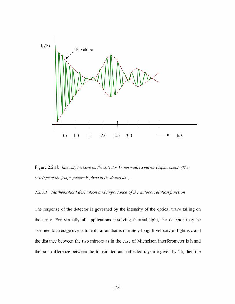
Figure 2.2.1b: Intensity incident on the detector Vs normalized mirror displacement. (The

envelope of the fringe pattern is given in the dotted line).

2.2.3.1 Mathematical derivation and importance of the autocorrelation function

The response of the detector is governed by the intensity of the optical wave falling on

the array. For virtually all applications involving thermal light, the detector may be

assumed to average over a time duration that is infinitely long. If velocity of light is c and

the distance between the two mirrors as in the case of Michelson interferometer is h and

the path difference between the transmitted and reflected rays are given by 2h, then the

Envelope ID(h)

0.5 1.0 1.5 2.0 2.5 3.0 h/λ

- 25 - 25

relative time delay is given by 2h/c. The intensity incident on the detector can be written

as

2

21 )2()()( ⎥⎦⎤

⎢⎣⎡ ++=

chtuKtuKhID - 2.1

where K1 and K 2 are real numbers determined

by the losses in the two paths. u(t) is the analytic signal representation of the light emitted

by the source. Expanding the expression we obtain an autocorrelation function. The

second wave is not a different entity; it could be the first wave at a different time. The

autocorrelation function measures the degree of coherence between the two waves. The

autocorrelation function is given by Γ(τ), and it plays an important role in determining the

observed intensity.

The autocorrelation function, which can be expressed through statistical expectation, can

be denoted by the following expression:

( ) )()( * tutu ττ +=Γ - 2.2

where u(t) is the analytic signal at time t, u(t+ τ) is the analytic signal at a time delay of τ

and u* is the complex conjugate. Note: Fourier transform of u(t) does not exist, in

general, because stationary random functions are not square integrable. Γ(τ) is also called

the self coherence function.

Now, the intensity detected at the detector, DI in general may be expressed as :

- 26 - 26

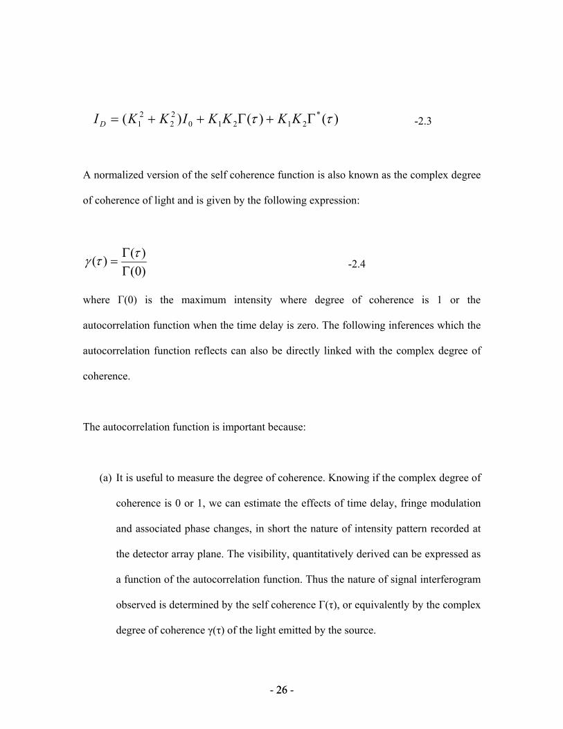
)()()( *21210

22

21 ττ Γ+Γ++= KKKKIKKI D -2.3

A normalized version of the self coherence function is also known as the complex degree

of coherence of light and is given by the following expression:

)0()()(

ΓΓ

=ττγ -2.4

where Γ(0) is the maximum intensity where degree of coherence is 1 or the

autocorrelation function when the time delay is zero. The following inferences which the

autocorrelation function reflects can also be directly linked with the complex degree of

coherence.

The autocorrelation function is important because:

(a) It is useful to measure the degree of coherence. Knowing if the complex degree of

coherence is 0 or 1, we can estimate the effects of time delay, fringe modulation

and associated phase changes, in short the nature of intensity pattern recorded at

the detector array plane. The visibility, quantitatively derived can be expressed as

a function of the autocorrelation function. Thus the nature of signal interferogram

observed is determined by the self coherence Γ(τ), or equivalently by the complex

degree of coherence γ(τ) of the light emitted by the source.

- 27 - 27

(b) For stationary random processes (a stationary process is a stochastic process

whose probability distribution at a fixed time or position is the same for all times

or positions and parameters such as the mean and variance, if they exist, also do

not change over time or position) an intimate relationship exists between the

autocorrelation function and the power spectral density of the source. The

Wiener–Khinchin theorem [51] (also known as the Wiener–Khintchine theorem

and sometimes as the Khinchin–Kolmogorov theorem) states that the power

spectral density of a wide-sense-stationary random process is the Fourier

transform of the corresponding autocorrelation function. Thus power spectral

density of the signal and the autocorrelation functions form Fourier transform

pairs.

( ) νντ πντ deS j∫∞

−=Γ0

2)(ˆ - 2.5

where S is the normalized power spectral density of the real-valued optical

disturbance. The normalized power spectral density has an unit area. If we know the

relationship between the autocorrelation function and power spectral density, the

form of the interferograms obtained with light having different shapes of the power

spectral density can be readily found out.

The Wiener–Khinchin theorem is useful for analyzing linear time-invariant (LTI)

systems when the inputs and outputs are not square integrable, so their Fourier

- 28 - 28

transforms do not exist. A corollary is that the Fourier transform of the

autocorrelation function of the output of an LTI system is equal to the product of the

Fourier transform of the autocorrelation function of the input of the system times the

squared magnitude of the Fourier transform of the system impulse response. This

works even when the Fourier transforms of the input and output signals do not exist

because these signals are not square integrable, so the system inputs and outputs can

not be directly related by the Fourier transform of the impulse response.

Since the Fourier transform of the autocorrelation function of a signal is the power

spectrum of the signal, this corollary is equivalent to saying that the power spectrum

of the output is equal to the power spectrum of the input times the power transfer

function.

(c) Since the character of an interferogram can be observed if the power spectrum is

known, it leads to the concept of Fourier spectroscopy. With the measurement of

the signal interferogram, if a FT is applied with several filtering techniques, one

can obtain the spectral signature; this idea is the basis of this research.

2.2.4 Fourier Transform Lens

The Fourier transform lens [16, 11, 15] plays a key role in the optics design as indicated

by the instrumentation name – Visible Fourier Transform Hyperspectral Imager. If the

interferogram has to be independent from aperture geometry requires that a pixel on the

- 29 - 29

detector array observe the same optical path difference induced by the interferometer

regardless of the position of an input source. If a lens with focal length l is placed

between the interferometer and the detector array exactly at a distance l from the detector

array this condition is met. First, consider the special case of the zero path difference

point as depicted in Figure 2.2.2a. We can show that if a detector is placed on the optic

axis of the lens and at a distance of one focal length from the lens, the optical path

difference is zero regardless of the separation or position of the two sources, as long as

the line which connects the sources is orthogonal to the optic axis. Consider a light source

placed at the center detector on the optic axis of the lens at a distance of f as depicted in

Figure 2.2.2a. We will observe, in the absence of aberrations, plane waves emerge from

the lens perpendicular to the optic axis. Each plane wavefront represents by definition a

contour of constant optical path length. At the original double source plane S (and any

plane perpendicular to the optic axis) any two sources fall on a contour of constant

optical path. As the optical distance from the center detector to any point on the constant

path contour is the same, there is no path difference between rays emanating from the two

sources and arriving at CD regardless of their separation or position. Now consider a

point P on detector plane F other than on the optic axis. Waves emitted from this off-axis

source would again emerge plane in an ideal optical system, but now will be inclined to

the optic axis by angle θ with tan θ equal to the distance from P to the optic axis divided

by f. The two sources on the input plane will now not lie on the same contours of

constant path, but will have a path difference Δ s sinθ , where s is the separation between

the sources. If the contours of constant optical path are plane then Δ will depend only

- 30 - 30

upon s and θ (defined by the point of observation P and the orientation of the sl s2 line),

and not upon the position of the pair along the input plane. Thus the only pairs of rays

which arrive at P from the sources will be those with path difference ‘Δ’. As the path

difference is independent of any translation of the sources, the interferogram generated

by this path difference and some source spectrum will also be independent of translation

of the source. Extending this result, any number of sources, in the limit an extended

source, will all produce the same path difference on any given detector, and each detector

will observe a different path difference. In this way the Fourier transform lens in

conjunction with the Sagnac interferometer produces an instrument which can obtain

spectra of extremely large fields of view. These characteristics allow the use of an

aperture of arbitrary geometry. While aberrations will limit the speed of the beam

actually employed and the pitch of the detector array, the position, size or shape of the

aperture will not affect the phase or frequency of the interferogram within the

assumptions of plane waves.

- 31 - 31

Figure 2.2.2a: Schematic of a Fourier Transform lens

Contours of optical path relative to a detector placed on the optical axis at one focal

length from the Fourier transform lens. A perfect lens yields plane contours. Sources on

any contour will yield zero path difference at the measurement point. The distance from

the source plane to the lens does not affect the path difference as long as the plane is

parallel to a contour of constant optical path. B) Contours of constant optical path from a

point P off the optical axis. The contours beyond the lens are still plane, but inclined to

the the normal to the optical axis by θ, where tanθ=P-CD/f. The path difference Δ equals

the source separation times sin θ, as long as the source plane remains normal to the optic

axis.

- 32 - 32

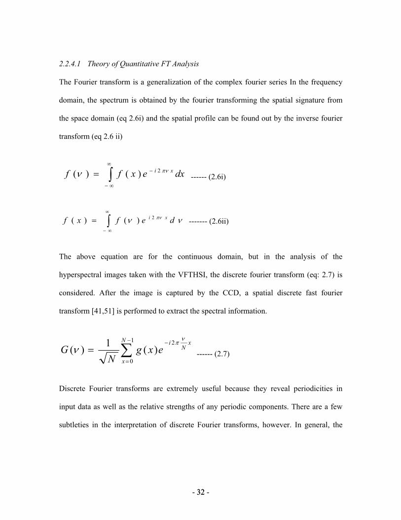
2.2.4.1 Theory of Quantitative FT Analysis

The Fourier transform is a generalization of the complex fourier series In the frequency

domain, the spectrum is obtained by the fourier transforming the spatial signature from

the space domain (eq 2.6i) and the spatial profile can be found out by the inverse fourier

transform (eq 2.6 ii)

dxexff xi∫∞

∞−

−= πνν 2)()( ------ (2.6i)

νν πν defxf xi∫∞

∞−

= 2)()( ------- (2.6ii)

The above equation are for the continuous domain, but in the analysis of the

hyperspectral images taken with the VFTHSI, the discrete fourier transform (eq: 2.7) is

considered. After the image is captured by the CCD, a spatial discrete fast fourier

transform [41,51] is performed to extract the spectral information.

∑−

=

−=

1

0

2)(1)(

N

x

xN

iexg

NG

νπ

ν ------ (2.7)

Discrete Fourier transforms are extremely useful because they reveal periodicities in

input data as well as the relative strengths of any periodic components. There are a few

subtleties in the interpretation of discrete Fourier transforms, however. In general, the

- 33 - 33

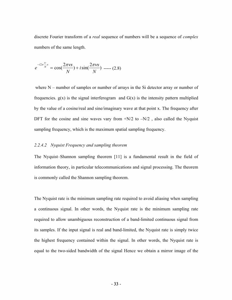
discrete Fourier transform of a real sequence of numbers will be a sequence of complex

numbers of the same length.

)2sin()2cos(2

Nxi

Nxe

xN

i πνπνυπ

+=−

----- (2.8)

where N – number of samples or number of arrays in the Si detector array or number of

frequencies. g(x) is the signal interferogram and G(x) is the intensity pattern multiplied

by the value of a cosine/real and sine/imaginary wave at that point x. The frequency after

DFT for the cosine and sine waves vary from +N/2 to –N/2 , also called the Nyquist

sampling frequency, which is the maximum spatial sampling frequency.

2.2.4.2 Nyquist Frequency and sampling theorem The Nyquist–Shannon sampling theorem [11] is a fundamental result in the field of

information theory, in particular telecommunications and signal processing. The theorem

is commonly called the Shannon sampling theorem.

The Nyquist rate is the minimum sampling rate required to avoid aliasing when sampling

a continuous signal. In other words, the Nyquist rate is the minimum sampling rate

required to allow unambiguous reconstruction of a band-limited continuous signal from

its samples. If the input signal is real and band-limited, the Nyquist rate is simply twice

the highest frequency contained within the signal. In other words, the Nyquist rate is

equal to the two-sided bandwidth of the signal Hence we obtain a mirror image of the

- 34 - 34

spectrum as depicted in the figures below which is symmetric in nature and the spectrum

from 0-N/2 is considered in order to retrieve the required spectrum.

By using a discrete FT, the interferogram intensity pattern is first sampled by low

frequency sine and cosine waves to see how the intensity pattern changed slowly across

the image. Then the pattern would be sampled at faster and faster frequencies until it

reaches the Nyquist sampling frequency limit of N/2. So, if the detector has 1024

channels, the spectrum will have 512 frequencies, also indicating the number of

bandwidths.

Fig 2.2.4.2 Shannon Sampling Theorem Depiction

(a)

-N/2 N/2

G(ν)

ν

- 35 - 35

(b)

If the input signal is real and band-limited, the Nyquist rate is simply twice the highest

frequency contained within the signal. In other words, the Nyquist rate is equal to the

two-sided bandwidth of the signal.

2.2.5 Cylindrical Lens

The cylindrical re-imaging optics [16, 28] is to ensure that the detector array is fully

illuminated; the placement of the input aperture and Fourier lens is such that the beam

emerging from the lens is roughly collimated. In short, the cylindrical optics lens takes

each the pixel in the spatial column limited by the input aperture and smears it into the

different frequency components equal to the arrays in the detector. The precise condition

is a function of the physical size of the detector, the speed of the beam, and the focal

-N/2 N/2

G(ν)

ν

- 36 - 36

length of the Fourier lens. When using a two dimensional detector array, each row would

contain the interferogram of the average spectrum of the input aperture. Introducing a

cylindrical lens of appropriate focal length near the Fourier lens, oriented such that it has

no power in the direction parallel to the line joining the input source pair (the

interferogram axis), serves to re-image the source along the axis parallel to the fringes

(constant path difference). This serves the dual of concentrating the radiation and

allowing resolved observations of targets along the axis perpendicular to the aperture.

The imager is now analogous to a slit spectrograph and the spatial information can be

obtained along the slit. Thus identical to a spectrograph, each row of the detector contains

the spectrum, in the form of the interferogram, of the corresponding point along the slit.

Unlike the spectrograph however the slit can be made arbitrary in width affecting the

resolution of the spectrum.

2.2.6 Silicon Detector

The CCD used in the VFTHSI is a CA-D4/D7 camera, which has a 1024 x1024

resolution with single 12-bit output (T model). Data for the 12-bit model is provided at

10MHz. This results in frame rates upto 8 frames/sec. The CA-D4/7 cameras use

DALSA’s patented modular architecture. Within the camera, a driver board provides

bias voltages and clocks to the CCD image sensor, a timing board generates all internal

timing, and A/D boards process the video and digitize it for output. Just as our eyes are

more sensitive to certain wavelengths so are some electronic light detectors. As shown in

- 37 - 37

the Figure below demonstrating the Silicon array detector response range, typically the

detector has a response curve that ranges from the longer mid-infrared wavelengths,

through the visible portion of the spectrum and into the shorter and also invisible

ultraviolet wavelengths. The most notable feature of the silicon detector's curve is its

peak sensitivity at about 900 nanometers. The VFTHSI CCD has a bandwidth range with

high sensitivity ranging from 450 – 950nm.

2.2.6.1 The Detector Array Design

The quantum efficiency of a photodetector [43] is defined as the number of electron-hole

pairs generated per photon. This quantity can be maximized by reducing the loss due to

reflections on the surface of the device and by increasing the absorbing region. P on P+

and P on N type epi-layer devices were fabricated with the same device layouts. The

photodetector array consists of 1024 elements which are read out in 16 channels of 64

pixels each. Each channel has an on-chip output amplifier which is designed to operate at

greater than 10 MHz. The pixel sizes are 30x30 microns which allows for an arrangement

which does not have even and odd pixel taps. Each of the 1024 photodetector elements in

the photosite array are separated by an anti-bloom barrier/ sink and covered by a

polycrystalline silicon photogate. Photons pass through the transparent photogate and are

absorbed in the single crystal silicon beneath it creating electron-hole pairs. The photo

generated electrons are stored under each photogate for a predetermined integration time

and then transferred in parallel into the CCD shift register. An image lag might occur if

the residual charge is held over to the next integration period, which also limits the small

- 38 - 38

signal detection of the array. To take care of this, all images are recorded with the same

integration time for equal exposure for all frames in the field of view. In order to

eliminate the noise generated by traps in the surface states formed during charge transfer,

a buried channel is implemented. In the buried channel, the charge resides in the bulk of

the material rather than at the surface which allows for improved transfer efficiency in the

device. Since surface-state trapping reduces charge transfer efficiency, a buried-channel

device is more desirable for high speed readout than a surface-channel device. For low

light levels, charge is accumulated in a potential well under the photogate. At the end of

the integration period all of the small signal charge is read out, resulting in a one-to-one

charge transfer curve. For light levels which exceed the well depth for the small signal

charge, the well is split by the sampling gate at the end of the integration period [43, 44]

and only a portion of the charge is transferred into the shift register. The rest of the

charge in the photosite is drained off into the anti-blooming drain. The large signal well

can continue to fill until it reaches the potential of the anti-blooming gate. At this point

the excess charge spills into the anti-blooming drain. A potential barrier formed by the

anti-blooming gate is used to separate the charge generated in the photosite from the anti-

blooming sink diode. When the potential of the charge exceeds the potential of the anti-

blooming gate, the charge is free to spill into the anti-bloom sink This type of structure

allows for the device to operate free from blooming at light intensities well above

saturation.

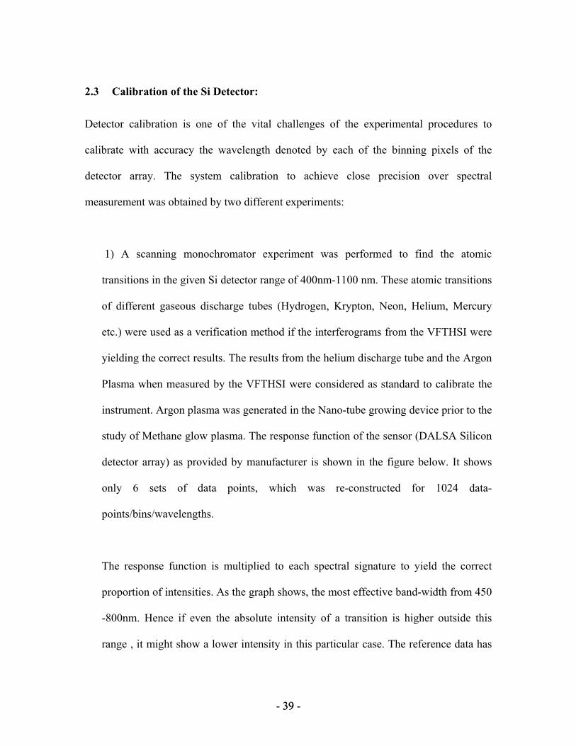
- 39 - 39

2.3 Calibration of the Si Detector:

Detector calibration is one of the vital challenges of the experimental procedures to

calibrate with accuracy the wavelength denoted by each of the binning pixels of the

detector array. The system calibration to achieve close precision over spectral

measurement was obtained by two different experiments:

1) A scanning monochromator experiment was performed to find the atomic

transitions in the given Si detector range of 400nm-1100 nm. These atomic transitions

of different gaseous discharge tubes (Hydrogen, Krypton, Neon, Helium, Mercury

etc.) were used as a verification method if the interferograms from the VFTHSI were

yielding the correct results. The results from the helium discharge tube and the Argon

Plasma when measured by the VFTHSI were considered as standard to calibrate the

instrument. Argon plasma was generated in the Nano-tube growing device prior to the

study of Methane glow plasma. The response function of the sensor (DALSA Silicon

detector array) as provided by manufacturer is shown in the figure below. It shows

only 6 sets of data points, which was re-constructed for 1024 data-

points/bins/wavelengths.

The response function is multiplied to each spectral signature to yield the correct

proportion of intensities. As the graph shows, the most effective band-width from 450

-800nm. Hence if even the absolute intensity of a transition is higher outside this

range , it might show a lower intensity in this particular case. The reference data has

- 40 - 40

been taken from NIST [6] and INSPEC. The data for Ar I (denoting the first

ionization of Argon) in the given spectral range is taken for reference.

The response function of the Si detector array or the sensitivity function was plotted

for each pixel. Different approaches were used to create the sensitivity function array,

for eg:- polynomial, logarithmic and power fits, but finally linear regression method

or interpolation was used to obtain the closest fit. The sensitivity plot (Fig 2.3 below)

was broken into 6 sections , with linear regression applied on each section. This

response function is multiplied to the spectral signature of plasma to obtain the right

intensities of the spectrum.

- 41 - 41

Response function (re-plotted)

0

5

10

15

20

25

30

35

40

45

50

400 500 600 700 800 900 1000

6-section linear regression

0

10

20

30

40

50

60

0 200 400 600 800 1000 1200

pixel

Inte

nsity

FIGURE 2.3a Showing Spectral Responsivity of the Detector

It is interesting to note that both the Fourier and inverse Fourier transforms on the

signal yield the same result. After inverse Fourier transform, we obtain a mirror

image of the spectra. I decided take the first 512 pixels (the 512th pixel denoting the

Nyquist frequency) as the spectral signature.

wavelength

- 42 - 42

The idea of linearity as considered before is wrong. If a standard He-Ne laser or

atomic transition of any gaseous discharge is taken for calibration , the pixel to

wavelength cannot be considered linear. The following reasoning is erroneous. If

there are N frequencies. Knowing λ, we can find wave number ν pix = 1/ λ at that pix

, and ν interval = ν / 512, ν Nyquist = ν interval * 512. If there are more than one transition

lines as in most cases, taking the difference between pixels and mapping that to

difference in wavelengths will generate erroneous results . Hence some assumptions

taken from the Response function along with the atomic transition data, a best

possible calibration was plotted as depicted in the graph below.

The data for conversion from pixels to wavelength was taken from (i) Helium spectra

taken from a gaseous discharge tube and few points from the response graph, (ii)

Argon Plasma spectra and few data points from the response graph. Hydrogen

spectra with two peaks at 656.28nm and OH peak at 777nm was also considered to

conform with the calibration data, but Helium and Argon owing to the presence of

more spectral lines gave better results.

(i) Helium spectra: The Interferometer was focused at the bulb portion of the

discharge tube to consider the atomic transitions ( He-I )of the strongest

- 43 - 43

electric fields. The transitions detected were at wavelengths 587.56nm,

501.5677nm and 447.147nm (Reference NIST data)

CALIBRATION GRAPH WITH HELIUM & DETECTOR RESPONSE DATA

y = 3E-05x2 + 1.176x + 393.57R2 = 0.9998

0

200

400

600

800

1000

1200

0 100 200 300 400 500 600

PIXEL

WA

VELE

NG

TH

Fig 2.3b: Calibration Graph with He & Detector response data

(ii) Argon Spectra:

When argon is used as a plasma gas, the emitted radiation is comprised mainly of lines of

the argon atomic spectrum [2] (Ar I). Molecular bands (e.g. OH, C2, N2, CN) observed if

a compound containing these species is injected into the plasma. The intensity of the

spectral lines observed in a defined observation zone depends on the plasma parameters.

Local thermal equilibrium does not usually exist in these plasmas. This implies that the

- 44 - 44

excitation mechanism of the analysis is not purely thermal. Argon atoms excited to

metastable levels seem to be of particular importance for all relevant processes in the

plasma. Electrons (up to ~30 eV), argon ions (argon ionization energy 15.76 eV) and

excited argon atoms play a major role in the processes.

The spectra shows the Argon –I lines (the first ionization state). The table below shows

the lines from NIST data.

Table 2.1. Ar –I Spectral lines observed with VFTHSI

NIST WAVELENGTH nm Relative Intensities

750.38 20,000

751.4 15,000

763.5 25,000

794.8 20,000

801.7 25,000

- 45 - 45

Fig2.3c: RF Argon plasma Spectral Analysis

2.4 Generating Hypercubes - analysis and examples

2.4.1 Experiments, Methods & Results

The Interferogram of the target image (fig 2.4a shows a 2-D 1024*1024 frame) is a 3-

dimensional matrix. There are two spatial dimensions including a customized scan

parameter to capture different frames of the target and one spectral dimension, which is

obtained after processing the data. Considering one of these frames ,we have a target

image ~(1024*1024 pixels) is captured and analyzed using the EPIX-XCAP software,

which generates the Interferogram with an excellent spatially modulated fringe pattern of

the target.

pix

I N T E N S I T Y

- 46 - 46

Figure 2.4a: (Right) 2-D Image Interferogram of white light,(Left) Filtered Signal Interferogram

plot a row of the target image.

Figure: 2.4b: (left) Signal and spectrum of a row of the He-Ne laser Target , (Right) Spatial Profile

of a column of He-Ne.

pix

I N T E N S I T Y

pix pix

- 47 - 47

2.4.2 Noise Reduction, SNR, & Filtering

The noise data is obtained by capturing dark frames with the same exposure

(5secs/frames). The Bias factor and photon noise are not included in the noise. Utilizing

Image Processing MATLAB simulations, the target and dark images are transformed into

matrices. The dark and flat-field are reduced by subtracting the dark data from target

image yielding the unfiltered signal interferogram (fig2.4c). Inverse imaging

computations are used find the spectrum by applying inverse Fourier transforms(Singular

Value Decomposition technique) to each row of the signal interferogram Adjustment of

VHTHSI for optimal setting is done initially to calibrate the instrument for the desired

experiment .Different resolutions attained by changing by the mirror orientation

associated with the cubical beam splitter of the Sagnac interferometer, altering the

visibility ,focusing and width of the fringe modulation , most noticeable at the Band Pass

region of the Si detector array. Calibration was essentially done by capturing white light

interferograms. The parametric study of Resolution versus SNR of VFTHSI agrees with

the SNR trade space, which was conducted to find the optimal instrument settings for a

reasonably good SNR value. When the fringes are wide, the interferogram intensity plot

spreads, spectrum becomes very narrow and we obtain a high SNR. The amplitude of

spectrum peak and SNR peak amplitude diminishes and broadens as the fringes are made

narrower generating high noise and low SNR. This is well depicted the graphs in Fig 2.4c

The target is a continuous function:-

∫∫ K(x,y)f(y)dxdy + η(x)=d(x) ---- (2.9)

- 48 - 48

where K Blurring Kernel (PSF) ,f(y)-object, d(x)-image , η-Noise. This is discretised to

Kf+ η=d ,where K-Square Matrix (1024*1024),K= USVT, S=diag(Si). Si– Eigen Values

of S. Singular Value Decomposition (SVD) technique is used to plot the spectrum, f=K-1

d

- K-1η. (a plot of PSD Eigen values), Spread in Eigen values causes noise amplification,

which makes the use of filters indispensable.

Figure 2.4 c: Parametric Study of SNR Vs Resolution

- 49 - 49

2.4.3 Generating the final Hypercube

The different scanned image frames are loaded as series of Interferograms. a) The code used is Tiff 2 ENVI, which is an executable file → generate header

&output file in ENVI

b) The first image frame shows the spatial distribution of FOV, x and y are the

spatial dimensions where x→ no.of rows in an image frame captured by EPIX-

XCAP/MATLAB , y → no. of scans across FOV.

c) The z-profile is the spectral distribution across the different bands or binning

pixels , which yields the spectral signature or chemical composition of the materials

present in that pixel. Z → no. of columns in an image frame captured by EPIX-

XCAP/MATLAB.

Spectra of pure gaseous discharge tube sources, obtained by a Monochromator

experimental set-up (instruments used gaseous discharge tube, high frequency chopper,

monochromator, detector, power supplies & Lock-in amplifiers) also serves as a target to

be correlated with the hypercubes using the same formalism. The ground based data-sets

of MTU and Houghton downtown are processed to obtain hypercubes (fig 2.4e) , which

is chiefly used for the correlation formalism in target recognition as elucidated in the

results.

A spectral profile mesh plot of all rows in a interferogram of a white light illuminated

target also produces a hypersurface plot as shown in fig 2.4d. The envelope indicates the

apodization function of the kernel.

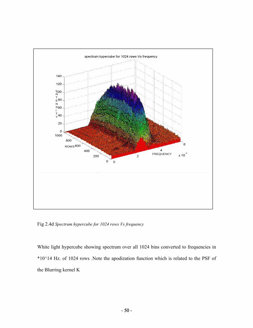
- 50 - 50

Fig 2.4d Spectrum hypercube for 1024 rows Vs frequency

White light hypercube showing spectrum over all 1024 bins converted to frequencies in

*10^14 Hz. of 1024 rows .Note the apodization function which is related to the PSF of

the Blurring kernel K

FREQUENCY

ROWS

INTENSITY

APODIZATION

INTENSITY

ROWS

FREQUENCY

- 51 - 51

Fig 2.4 e :Hypercubes of two different aerial targets.(Above)-Downtown, Houghton-122spectral bands

RGB-48,26,17.(Below)- Hypercube showing Michigan Tech-150 spectral Bands,RGB-98,87,25 is chiefly

used to obtain the results in the correlation formalism.

- 52 - 52

Chapter 3

3 PHYSICALLY MOTIVATED CORRELATION FORMALISM (PMCF)

3.1 Methodology

The objective of this section is to address the question of how best or optimally the entire

Hypercube can be sampled for a better target recognition process. This approach is based

on the basic attributes of information theory and the information content of indirect

sensing measurements.

A variety of techniques have been utilized in attempts to exploit hyper-spectral data.

These may be simplistic but intuitive techniques that include band averaging, band

rejection, spatial averaging, or just mind-numbing number crunching. More sophisticated

attempts to exploit the data volume of the hypercube include pattern recognition, end-

member analysis, spectral mapping, spatial sharpening, and similarity transformations. It

has been more emphasized about how many spectral bands are needed to recognize a

target, with less attention to the symmetric question how much spatial resolution is

required. Very little or no attention to the fundamental question of how many (spatial-

spectral) pixels may be needed to detect a target of specific interest. To answer this

problem, I designed a physically motivated correlation formalism or PMCF [5], which

places spatial and spectral information on an equal mathematical footing in the context of

- 53 - 53

a specific application (kernel), with the objective of finding the optimal (independent) set

of spatial/spectral measurements within the entire hypercube (Fig 3.1). These

independent spectral measurements (spectral signature) can assist in building spatial

content, in the same way that spatial content (pattern recognition) can be utilized to refine

spectral content. In its full implementation, PMCF is not just a spectral endmember

technique, or an equivalent spatial end-member technique but in a simplified statement,

the equivalent of both taken together.

In many real problems, there are a limiting and usually small number of independent

measurements, beyond which there is no effective increase in information content. Even

an increase in the number of observations may not offer a positive contribution, if errors

(noise) exceed threshold levels. These physical constraints of obtaining high SNR levels,

while not reducing the number of measurements (e.g., spectral bands) to unacceptably

small values.

Consider g(x,y,λ) for (n,m,l) values of x,y,λ , of which (N,M,L) are independent

measurements. So if

g (x,y,λ)= ∫ ∫ ∫ K (x,y,λ) f(x,y,λ)dx dy dλ+ η(x,y,λ) ------- (3.1)

where g(x,y, λ ) is the image, K(x,y, λ) is the spatial/spectral Kernel, η(x,y, λ) is the noise

and f(x,y, λ) is the spatial/spectral target, a key point is that the eigenvectors/endmembers

of the inverse problem depend on the noise, and hence, on the various ways in which

correlated pixels within the hypercube can be averaged to increase the number of useful

- 54 - 54

eigenvalues. Investigators usually assume orthogonality and normalization of the data but

often fail to discard terms whose contribution is small compared to the error noise (which

as we note below, can be substantial if flawed processing techniques or poor data

reduction strategies are employed). This follows from the well known result that the

number of non-redundant independent pixels in the set g(x,y, λ) is the number of

eigenvalues in the covariance matrix that exceed the average square norm of the errors in

g(x,y, λ).

PMCF supplies the tool that selects and/or groups pixels within the hypercube to

maximize the number of independent pixels, via determination of parameter correlations,

for a specific target(s). Of course, even simplistic spectral or spatial averaging would

reduce the magnitude of the ‘errors’, but with a guarantee of removing independent

information from some image or spectral pixels. Key to the success of any effort is the

ability of the analysis to find independent pixels that define target attributes, as opposed

to just a simplistic computation of endmembers.

- 55 - 55

3.1.1 Correlation Moments

Of particular interest in establishing the best procedure for this process is the

determination of the optimal role of the Primary and Secondary correlation moments

involving different pixels I(i,j,k) in Fig 3.1,where i=1:1024,j=1:1024,k= # of bands, that

we define as follows:

Primary Moment I

1st Spectral Moment [Ms1] is a spectral -spectral correlation of 2 spectral profiles –

pixel(s) I(xi, yj, λ[1:k]) with pixel(s) I(xi+δ, yj+δ, λ[1:k])

1st Spatial Moment[Msp1] is a spatial-spatial correlation of 2 spatial profile—

pixel(s) I(xi, y[1:j], λk) with pixel(s) I(xi+δ, y[1:j],λk) or I(x[1:i],yj, λk) with I(x[1:i], yj+δ,

λk).

Primary Moment II 2nd (Spectral/Spatial) Moment— MII, correlation of spectral with a spatial profile correlation of pixel(s) I(xi, yj, λ[1:k]) with I(xi+δ, y[1:j],λk) or I(xi, yj, λ[1:k]) with I(x[1:i], yj+δ, λk).

Secondary Moment I 3rd Cross correlation Moment between non-adjacent / cross pixels –MIII.

Fig 3.1: hypercube with x,y, λ profiles

X profile

Λ profile

Y profile

- 56 - 56

3.2 Correlation Results

Applying standard cross-correlation method, we can estimate the degree to which 2

spectral profiles or spatial profiles are correlated, incorporating a new parameter ‘delay’

where the delay varies from –Max Band # to + Max Band # and the Max Band # is the

last bin/wavelength in the Band Pass.

The cross correlation r at delay d is :

………….. 3.2

x(i) – Spectral profile of each spatial bin in the selected ROI, y(i)- Spectral profile of

target , where i=0,1,2,3…N-1. Where mx subscript and my subscript are the means of the

corresponding spectral profiles. The above is computed for all delays d=0,1,2,...N-1,so

that it results in a cross correlation series of twice the length as the original series. The

maximum correlation value of each correlation array is plotted in a 3-D histogram. Refer

the plot in Fig (3.2) The chosen water pixel shows strong correlation with most pixels of

identical nature, with the strongest at the point of occurrence of itself. Similarly, the

correlation of any target can be estimated with the hypercube.

There is the issue of what to do when the index into the series is less than 0 or greater

than or equal to the number of points. (i-d < 0 or i-d >= N). Using wrap around theory,

we use the following correlation equation in such a case. r(d)= ∑[(x(i)-mx)*my] /

√∑(x(i)-mx)2√∑(y(i)-mx)2

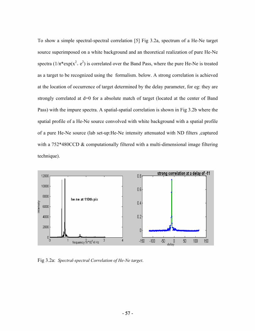
- 57 - 57

To show a simple spectral-spectral correlation [5] Fig 3.2a, spectrum of a He-Ne target

source superimposed on a white background and an theoretical realization of pure He-Ne

spectra (1/π*exp(x2+ e2) is correlated over the Band Pass, where the pure He-Ne is treated

as a target to be recognized using the formalism. below. A strong correlation is achieved

at the location of occurrence of target determined by the delay parameter, for eg: they are

strongly correlated at d=0 for a absolute match of target (located at the center of Band

Pass) with the impure spectra. A spatial-spatial correlation is shown in Fig 3.2b where the

spatial profile of a He-Ne source convolved with white background with a spatial profile

of a pure He-Ne source (lab set-up:He-Ne intensity attenuated with ND filters ,captured

with a 752*480CCD & computationally filtered with a multi-dimensional image filtering

technique).

Fig 3.2a: Spectral-spectral Correlation of He-Ne target.

delay

- 58 - 58

The pure He –Ne is located at 110th pix (.87*1014 Hz.) at one end of the Band Pass of the

spectra of He-Ne+white screen. The correlation is maximum at a delay of -11 as

expected.

Fig 3.2 b: Spatial-spatial correlation of He-Ne source

3.2.1 PMCF using MTU images (Spectral Matching)

A spectral library (fig 3.2c) created has spectral profiles of one spatial pixel over all the

bands/spectral bins within the Band Pass (of the Si detector array) or average of a group

of pixels from the selected ROIs. This spectral library showing spectral profiles of

different targets (fig 3.2c) is considered as a chosen target and is correlated with a

particular region of interest containing the target in hypercube. For eg: An AOI

(40row*70columns*150Bands) - marked in white as shown in Fig (3.2e) is selected in the

hypercube showing MTU such that it covers all the chosen spectral libraries to be

correlated. This AOI is stored as arrays with each array containing one spatial pixel over

pix delay

- 59 - 59

the entire Band Pass (524nm-1021nm). This hypercube is now correlated with the target

spectrum using cross-correlation involving a delay parameter d which runs from ‘-’ Max

band to # ‘+’ Max band #. For eg: Target chosen is from a water spectral library, which is

correlated with the AOI over a delay of -150 to +150, shows strongest correlations with

the water pixels.

Fig 3.2c Spectral Library plots in ENVI of water, sky, buildings & greenery

Fig 3.2c shows spectral library plots in ENVI of water, sky, buildings & greenery (above)

and how each of the spectral libraries are correlated with the spectral profile of a water

pixel, which shows the maximum correlation with another water spectral library at a

delay of zero & at different delays (-ve or +ve) with other spectral libraries like sky,

buildings & greenery (below) in figure 3.2d.

sky

building

water

greenery

- 60 - 60

0 50 100 150 200 250 300 350-1

-0.8

-0.6

-0.4

-0.2

0

0.2

0.4

0.6

0.8

1Cross-Correlation graph

watertreesskybuildings

Fig 3.2d: Cross Correlation Graph

Fig 3.2e: Selected AOI within MTU Hypercube with 150 bands

delay

- 61 - 61

Fig 3.2f: Correlation mesh-plots of all arrays in the AOI and a water pixel spectra from the

spectral library.

Fig below shows 3-D histogram showing the Maximum value of correlation between

water pix and all other arrays containing spectral signatures of the pixels in the selected

AOI (40rows, 70cols). The maximum correlation location is the point of occurrence of

the target water pixel.The high correlation values portrays water pixels of similar nature

in the AOI.

- 62 - 62

Fig 3.2g: 3-D histogram showing the Maximum value of correlation between water pix and all

other arrays containing spectral signatures.

Similarly, a spatial-spatial Correlation is also computed with the area of interest in the

hypercube , which estimates the degree of correlation between adjacent rows or colums

and also enables a spatial target recognition . The full development of the possibilities

afford by the use of PMCF lays beyond the scope of this paper, whose primary focus

includes the development of the data sets and basic analysis strategies that will be used in

subsequent investigations.

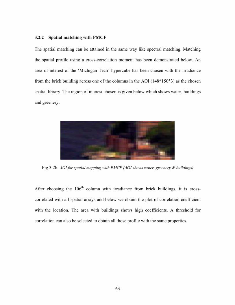
- 63 - 63

3.2.2 Spatial matching with PMCF

The spatial matching can be attained in the same way like spectral matching. Matching

the spatial profile using a cross-correlation moment has been demonstrated below. An

area of interest of the ‘Michigan Tech’ hypercube has been chosen with the irradiance

from the brick building across one of the columns in the AOI (148*150*3) as the chosen

spatial library. The region of interest chosen is given below which shows water, buildings

and greenery.

Fig 3.2h: AOI for spatial mapping with PMCF (AOI shows water, greenery & buildings)

After choosing the 106th column with irradiance from brick buildings, it is cross-

correlated with all spatial arrays and below we obtain the plot of correlation coefficient

with the location. The area with buildings shows high coefficients. A threshold for

correlation can also be selected to obtain all those profile with the same properties.

- 64 - 64

0

20

40

60

80

100

120

140150-0.4

-0.2

0

0.2

0.4

0.6

0.8

1

-1

-0.5

0

0.5

1

Fig 3.2i: PMCF coefficient Vs Col Location for spatial mapping.

After mapping the histogram plot to the area of interest we obtain the following figure,

which makes visualization of spatial matching simpler.

Correlation Col Location

- 65 - 65

Fig 3.2j: Spatial mapping with PMCF (Correlation Mapping area mapped to the chosen AOI)

- 66 - 66

3.3 Conclusions

After careful consideration, I am negating the scope of correlating a spectral profile with

a spatial profile. The axes of these profiles are different- one of them focuses on the

number of bins or wavelengths, while the other is just an intensity graph with the x-axis

consisting of the cell counter and not bin. These disjoint profiles, when correlated

together will not generate anything that may be of meaningful physical interpretation. But

presenting a spectral correlation of a chosen area of interest with a target spectral library,

which may be presented as 3-D histogram indicating the cell where a high correlation

occurs gives us the spectral matching point and one can easily find out the location of the

target spatially through this representation. Hence analysis of secondary moments are not

being demonstrated since any physically meaningful information may not be extracted

from the analysis.

Ruling out spatial-spatial correlation on the other hand may not be interesting since based

in spatial intensity matching by the correlation formalism, it is possible to find out the

target pixel effectively. The spatial/spatial matching is easily observed when there is only

one component (say an hypercube from a He-Ne laser), but when a complicated

hypercube such as the Houghton hypercube is exploited, it is difficult to observe the

target with the spatial/spatial matching. I have demonstrated the spatial/spatial matching,

which is also a primary moment in this section.

- 67 - 67

The physically motivated formalism in hyperspectral imaging is one of the most

sophisticated methodologies in Signal Processing to sample the entire Hypercube data

both spectrally and spatially very effectively. Correlation Moments I showing

spectral/spectral or spatial/spatial correlations can be easily computed by this technique.

As observed in the Results section PMCF especially enables any spectral or spatial target

recognition very efficiently with precision.

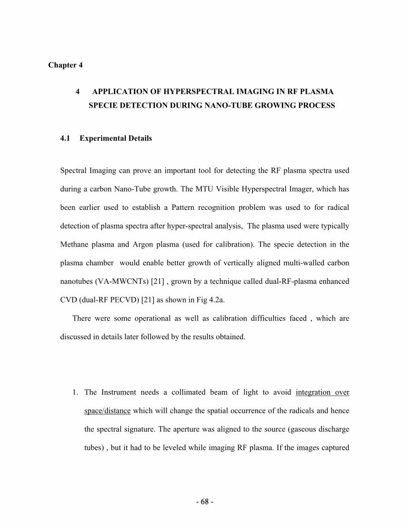
- 68 - 68

Chapter 4

4 APPLICATION OF HYPERSPECTRAL IMAGING IN RF PLASMA

SPECIE DETECTION DURING NANO-TUBE GROWING PROCESS

4.1 Experimental Details

Spectral Imaging can prove an important tool for detecting the RF plasma spectra used

during a carbon Nano-Tube growth. The MTU Visible Hyperspectral Imager, which has

been earlier used to establish a Pattern recognition problem was used to for radical

detection of plasma spectra after hyper-spectral analysis, The plasma used were typically

Methane plasma and Argon plasma (used for calibration). The specie detection in the

plasma chamber would enable better growth of vertically aligned multi-walled carbon

nanotubes (VA-MWCNTs) [21] , grown by a technique called dual-RF-plasma enhanced

CVD (dual-RF PECVD) [21] as shown in Fig 4.2a.

There were some operational as well as calibration difficulties faced , which are

discussed in details later followed by the results obtained.

1. The Instrument needs a collimated beam of light to avoid integration over

space/distance which will change the spatial occurrence of the radicals and hence

the spectral signature. The aperture was aligned to the source (gaseous discharge

tubes) , but it had to be leveled while imaging RF plasma. If the images captured

- 69 - 69

by the VFTHSI are expressed as matrices , then the zone containing the plasma

data can be represented as:

n

nn

Nn

xxxxx

xxxxxxxxx

1

1

.........321..........321.........321

−

−

The time of capture was also increased from 100ms to 0.5 secs to enhance photon

capture. Hence it was asserted there is integration over time.

2. The system is designed specially for remote sensing applications with targets

located at infinity it was very essential to ensure that the rays from the target re

not obliquely incident on the imager, but are parallel. This was established when 2

different spectral signatures were generated from the Hydrogen discharge tube in

case i) parallel incidence ii) oblique incidence .

3. It should be noted that the atomic transition should be retained from the narrow

section of the discharge tube when the electric field is the strongest. The spectra

taken from the bulb-like part of the tube may result in errors as it mainly consists

of molecular transitions.

4. The VFTHSI was used to take hydrogen, helium, argon, krypton data from

discharge tubes mainly for the purpose of calibration.

We would want our signal to be a linear combination of the elements of any row and not off-diagonal terms (for eg: the boxed terms) of the matrix which will change with the angular positions of the aperture with respect to the axis perpendicular to the masking slit.

- 70 - 70

5. The Image analysis with one plasma (i.e plasma generated around one electrode)

or fluctuating pressure inside the chamber will invariably result in erroneous

results in the determining the spectral signatures.

4.2 The R-F Dual Plasma Source Description

Carbon nanotubes (CNTs) are among the promising materials that are expected to play a

major role in the future of nanoscience and nanotechnology. Their unique structural and

electronic properties have made them a potential candidate for many nano-electronic,

mechanical, chemical, and biological applications. Vertically aligned multi-walled carbon

nanotubes (VA-MWCNTs) is grown by a technique called dual-RF-plasma enhanced

CVD (dual-RF PECVD), which is operated with two RF plasmas. One of the plasma is

used to decompose the methane (CH4) gas and plasma is used to initiate substrate bias

voltages that can accelerate the growth species at a controllable kinetic energy. The dual-

RF-CVD chamber is shown in Fig 4.2b. The plasma produced by the top RF generator is

called the top plasma, whereas the plasma produced by the bottom RF generator is called

the bottom plasma. The top plasma is adjusted according to the forward RF power

requirement, while the bottom plasma is controlled by adjusting the bias voltage on the

adjusting the bias voltage resulting on the substrate. The change in forward plasma power

results in different decomposition rates of the methane gas. The decomposition of the

methane gas results in the creation of positive carbon and hydrocarbon ions (C+, CH+, H+

- 71 - 71

etc.), electrons, neutral molecules and radicals. The positive ions are accelerated towards

the substrate by the negative bias voltage that is adjusted by the bottom plasma power.

The use of two RF-power sources in the technique allowed us to examine the effects of

positive ion bombardment on the formation of MWCNTs. The two plasma frequencies

are in isolation from one another as the two electrodes are far apart from each.

requirement, while the bottom plasma is controlled by adjusting the bias voltage resulting

on the substrate. The change in forward plasma power results in different decomposition

rates of the methane gas. The decomposition of the methane gas results in the creation of

positive carbon and hydrocarbon ions (C+, CH+, H+ etc.), electrons, neutral molecules and

radicals. The positive ions are accelerated towards the substrate by the negative bias

voltage that is adjusted by the bottom plasma power.

The two factors [1], which are crucial in determining the plasma specie densities are

(i) Incident RF power

(ii) Pressure

Also, as the magnetic field inside the plasma source increases, there is a rise in the radical

densities. The spectral intensity ratios obtained from different known literature is

different owing to the instrument response function. The spectrum obtained from the

interferogram is multiplied to the Dalsa Silicon detector sensitivity or response function.

- 72 - 72

Conditions under which the Methane plasma (Fig 4.2a) was imaged:

1. The top plasma generated by RF power ~ 150 Watt

2. Bottom plasma generated by D.C source ~150 D.C

3. Pressure in the Chamber ~ 0.2 Torr

Though the number densities of the CH4 plasma radicals changes as the RF forward

bias is altered from 100-300 W, but the specie spectra remains unaltered. The

electrode spacing can also change the radical densities. Fig 4a below shows Methane

glow plasma between the two electrodes.

- 73 - 73

Fig 4.2a: PE- CVD chamber (showing top and bottom plasma around electrodes)

Figure 4.2b: Experimental setup of the dual RF-PECVD chamber

Top plasma generator

Bottom plasma generator

Temperature controller

Thyristor

Coolant (water)

Methane supply (a)

- 74 - 74

As reported in most literature,

the radicals found are :-- CH,

H, H2

Refer table- 4.1 above to find

commonly found species.

Table 4.1. RF Methane Plasma Spectral Lines.

4.3 Calibration using RF Argon Plasma

The main challenge was to calibrate the system accurately to achieve close precision over

spectral measurement.

The calibration was achieved by two different experiments:

1) A scanning monochromator experiment with emission spectra from helium

discharge tube taken as a standardized spectral signature. The experiment was also

performed to find the atomic transitions in the given detector range of 400nm-900 nm of

different gaseous discharge tubes (Hydrogen, Krypton, Neon, Helium ,Mercury etc.) ,

Specie Wavelength(nm)

CH 428.6 nm

Hβ 484.5 nm

Hα 656.2nm

Swan bands 310.8nm-387.3nm

Hδ 406.4 nm

Hγ 433.3

Molecular hydrogen 463 nm & 602nm

- 75 - 75

which were used as a verification method if the interferograms from the VFTHSI were

yielding desired results

2) The second reference spectra for calibration was from RF Argon plasma [23],

which was generated in the RF plasma generating device prior to the study of Methane

glow plasma.

Procedure of Instrument Calibration The response function of the sensor (DALSA Silicon detector array) as provided by

manufacturer is shown in the figure below. It shows only few sets of data points, which

was re-constructed for 1024 data-points /bins/wavelengths. The response function of the

Si detector array or the sensitivity function was plotted for each pixel with an approach of

linear regression method or interpolation (the sensitivity plot was broken into 6 sections

regression) to obtain the closest fit to the Dalsa quantum efficiency.

The response function is multiplied to each spectral signature to yield the correct

proportion of intensities in the RF plasma spectra. As the graph in Fig 4.3a shows the

most effective Band-width from 450 -800nm, hence if even the absolute intensity of a

transition is higher outside this range , it might show a lower intensity in this particular

case. The reference data has been referred from a standardized database for atomic lines

in Ar I ( neutral atoms) and Ar(II) or Ar+ (denoting the first ionization of Argon) in the

given spectral range is taken for reference.

- 76 - 76

Response function (re-plotted)

0

5

10

15

20

25

30

35

40

45

50

400 500 600 700 800 900 1000

6-section linear regression

0

10

20

30

40

50

60

0 200 400 600 800 1000 1200

pixel

Inte

nsity

FIGURE 4.3a Showing Spectral Response

A Note in VFTHSI Calibration

The linearity consideration of wavelength/pix calibration in Reference6), which says if

there are N frequencies, then knowing λ, we can find wave number ν pix = 1/ λ at that pix

, and ν interval = ν / 512, ν Nyquist = ν interval * 512 or if there are more than one transition

lines as in most cases, taking the difference between pixels and mapping that to

difference in wavelengths will generate slightly erroneous results . Hence some

- 77 - 77

assumptions taken from the Response function along with the atomic transition data , a

best possible calibration was plotted as depicted in the graph below (Fig 4.3a)

The data for conversion from pixels to wavelength was taken from (i) Helium spectra

taken from a gaseous discharge tube and few points from the response graph , (ii) Argon

Plasma spectra and few data points from the response graph. Hydrogen spectra from

gaseous discharge tube with a peak at 656.28nm and Oxygen line at 777nm was also

considered to conform with the calibration data, but Helium and Argon owing to the

presence of more spectral lines gave better results.

(iii)Helium spectra: The Interferometer was aligned at the bulb portion of the

discharge tube to measure the atomic transitions [6] ( He-I )of the strongest electric

fields. The transitions detected were at wavelengths 587.56nm, 501.5677nm and

447.147nm.

(iv) The graph (Fig 4.3bi) below shows helium spectra measured with the VFTHSI

with a scanning Monochromator set-up3) and the three intense lines correspond to the

wavelengths stated above and then by regression method, a calibration relation is

established as stated in the graph (Fig 4.3bii) with regression coefficient =0.9998.

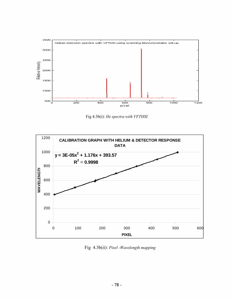
- 78 - 78

Fig 4.3b(i): He spectra with VFTHSI

CALIBRATION GRAPH WITH HELIUM & DETECTOR RESPONSE DATA

y = 3E-05x2 + 1.176x + 393.57R2 = 0.9998

0

200

400

600

800

1000

1200

0 100 200 300 400 500 600

PIXEL

WA

VELE

NG

TH

Fig 4.3b(ii): Pixel -Wavelength mapping

- 79 - 79

(ii) RF Argon Spectra:

When argon is used as a plasma gas [1, 6] the emitted radiation is comprised mainly of

lines of

the RF-argon atomic spectrum (Ar I). The gas injected was pure Argon and since no

other species were injected into the chamber, molecular bands (e.g. OH, C2, N2, CN, N+)

were not observed. The intensity of the spectral lines observed in a defined observation

zone depends on the plasma parameters. Local thermal equilibrium does not usually exist

in these plasmas. This implies that the excitation mechanism of the analysis is not purely

thermal. Argon atoms excited to metastable levels seem to be of particular importance

for all relevant processes in the plasma. Electrons (few electron Volts, 3~4 eV), argon

ions (argon ionization energy 15.76 eV) and excited argon atoms play a major role in the

processes.

Figure 4.3c shows Interferogram of RF Argon Plasma in PECVD chamber (Target

Signal) of a particular scan shot.

Fig 4.3c: Interferogram of RF Argon Plasma in PECVD chamber

- 80 - 80

The spectra show the Argon –I lines (neutral atomic state) [6]. The table below shows the

lines from NIST. Fig 6.7 shows the Ar I spectra (i) at the central part of the RF plasma

glow (ii) close to the interface between top electrode and plasma glow (ii) close to the

interface between bottom electrode and plasma glow. Fig 4.3d shows all lines of strong

intensities as tabulated in table 4.2. The line at 811nm has overlapped with the line at

801nm and though the relative intensity at 811nm is higher, it is lower or comparable to

801nm in the fig 4.3d owing to the diminishing response function of the detector.

Table 4.2. RF Argon plasma lines

NIST WAVELENGTH nm Relative Intensities

750.38 20,000

751.4 15,000

763.5 25,000

794.8 20,000

801.7 25,000

811.53 35,000

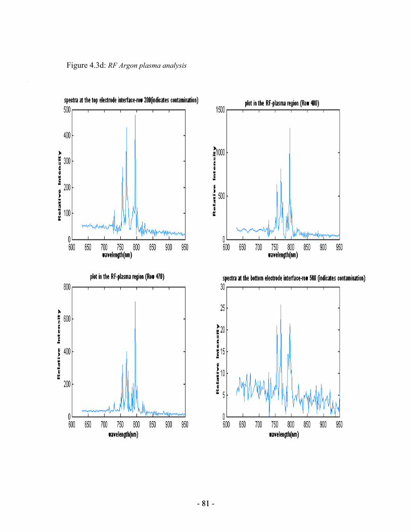
- 81 - 81

Figure 4.3d: RF Argon plasma analysis

- 82 - 82

4.4 Results of Hyperspectral Analysis of RF CH4 Plasma

Procedure: The VFTHSI was taken out of the Meade stand and placed parallel to the

plasma window to prevent integration over space. The slit was wide opened to maximize

the number of photon capture since we were dealing with a dim source here. Normally

the VFTHSI is designed for targets at infinity (Remote sensing), but for it’s high

resolution of 1.13nm, it is extremely advantageous for precise spectral measurements. It

negates the elaborate experimental set-up with many optical fiber probe coupled

spectrometer [24], since each image frame (FOV) can be easily used to see the spectral

distribution. The Signal Interferograms are filtered, convolved with the response

function, following which a inverse fast Fourier transform is performed to yield the RF

methane plasma glow spectra as depicted in graph 4.4d.

The calibration conversion used was y = -0.0017x^2 + 1.9824x + 107.02, R^2 = 0.9738,

where R presents regression coefficient.

- 83 - 83

A detailed study of different high intensity atomic transitions along with different

molecular bands as described above has been shown in graph 4.4d, we obtained presence

of mono-atomic and di-atomic species within the methane plasma.

Hypercube creation with plasma Interferograms: 3-D hypercubes with the plasma data

were generated when the methane RF-plasma was scanned. Each scanned frame looked

like Fig 4.4c and when when loaded up as hypercubes in ENVI, it enables us:

Figure 4.4a(Top): Plot of Two Rows of Signal Interferograms of the CH4 glow plasma plotted in Epix-Xcap. The # of photons (Plasma Intensity)is very large within pixels 400-900. Figure 4.4b(Left). The Interferogram Image of Methane Plasma as captured under customized conditions by the VFTHSI

- 84 - 84

1. To find the spectra of any spatial point in between the two electrodes easily

utilizing the software ENVI as the spatial location of radical differ over temporal

changes.

2. Temporal Changes: Gives an estimation of specie density change or radical

change spatially and spectrally with time.

3. The different spectral signatures will help see the correlation between different

kinds of nano-tubes grown (Figure 4.4e shows carbon nano-tube growth)

Fig 4.4c: Interferogram of a frame during scanning of CH4 RF-plasma.

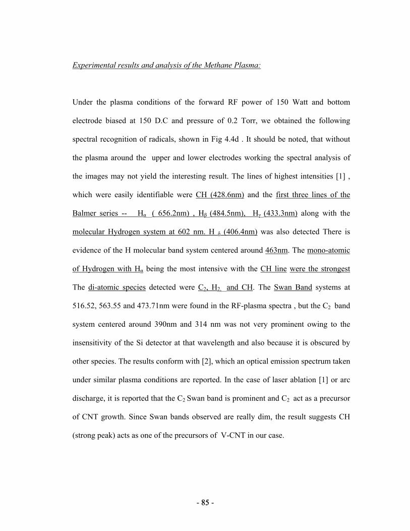
- 85 - 85

Experimental results and analysis of the Methane Plasma:

Under the plasma conditions of the forward RF power of 150 Watt and bottom

electrode biased at 150 D.C and pressure of 0.2 Torr, we obtained the following

spectral recognition of radicals, shown in Fig 4.4d . It should be noted, that without

the plasma around the upper and lower electrodes working the spectral analysis of

the images may not yield the interesting result. The lines of highest intensities [1] ,

which were easily identifiable were CH (428.6nm) and the first three lines of the

Balmer series -- Hα ( 656.2nm) , Hβ (484.5nm), Hγ (433.3nm) along with the

molecular Hydrogen system at 602 nm. H δ (406.4nm) was also detected There is

evidence of the H molecular band system centered around 463nm. The mono-atomic

of Hydrogen with Hα being the most intensive with the CH line were the strongest

The di-atomic species detected were C2, H2, and CH. The Swan Band systems at

516.52, 563.55 and 473.71nm were found in the RF-plasma spectra , but the C2 band

system centered around 390nm and 314 nm was not very prominent owing to the

insensitivity of the Si detector at that wavelength and also because it is obscured by

other species. The results conform with [2], which an optical emission spectrum taken

under similar plasma conditions are reported. In the case of laser ablation [1] or arc

discharge, it is reported that the C2 Swan band is prominent and C2 act as a precursor

of CNT growth. Since Swan bands observed are really dim, the result suggests CH

(strong peak) acts as one of the precursors of V-CNT in our case.

- 86 - 86

Importance of HSI technique in spectral detection of plasma chemistry:

HSI as discussed before gives detailed ,precise (1.13nm precision) and rapid

information about CH4 RF-plasma composition as the spatial location of specie

occurrence change with time. This spectral information is very useful in growing

vertically oriented carbon nano-tubes (V-CNTs) –Fig 4.4d, which have applications

as cold cathodes, quantum wires for nano-scale devices , tips for scanning &

biological probes. There lies a strong correlation between the plasma state and

structural property in the growth of V-CNTs [1]. The plasma diagnostics in the

PECVD depend on the forward RF power, VD.C (self-bias)and the pressure. As these

parameters change plasma chemistry changes . The structural properties of V-CNTs

are significantly correlated with the fractions of H atoms or radicals , CH radicals and

VD.C , which increase with increasing RF power. It is suggested [1, 2] that during V-

CNT growth, the H species act as etchants, while the CH radical acts as a precursor of

the growth. These antagonistic factors influenced the structural properties of V-CNTs

yielding an optimum RF power for the growth of V-CNTs with very good

crystallinity [24]. The crystalline properties can be tested easily with this HSI

technique of specie recognition to generate very high quality CNTs.

- 87 - 87

Figure 4.4d: Hyperspectral Analysis of Methane RF-Plasma Spectra .

- 88 - 88

Figure 4.4e:

SEM image[21] of

grown VA-MWCNTs

using the dual- RF PECVD

4.5 Plasma Analysis Conclusions

The physically motivated formalism in hyperspectral imaging is one of the most

sophisticated methodologies in Signal Processing to sample the entire Hypercube data

both spectrally and spatially very effectively. Correlation Moments I showing

spectral/spectral or spatial/spatial correlations can be easily computed by this technique.

As observed in the Results section PMCF [5] especially enables any spectral or spatial

target recognition very efficiently with precision.

The Spectral signature detection with Hyperspectral Fourier Transform Imaging to

recognize the radicals/species of Methane RF-Plasma was successfully accomplished,

- 89 - 89

which will result in a strong correlation with the structural properties of Carbon Nano

tubes. With the Hypercube generation and analysis the temporal changes of the plasma

state & densities can be easily mapped for better crystal properties of CNTs.

To summarize, the following are the key points of this research:

• The Spectral signature detection with Hyperspectral Fourier Transform Imaging to

recognize the radicals/species of Methane RF-Plasma was successfully accomplished

• It rapidly shows the correlation between plasma composition & structural properties

of Carbon Nano tubes.

• With Hypercube generation and analysis the temporal changes of the plasma state &

densities can be easily mapped for better crystal properties of CNTs.

- 90 - 90

Chapter 5

5 ERROR ESTIMATION IN AN ILL-CONDITIONED INVERSE IMAGING

PROBLEM OF REFLECTANCE

In the previous chapters, I have demonstrated areas of hyperspectral application, like the

PMCF in examining remote sensing data or capturing the temporal changes of spectral

signature of the methane plasma species during the growth of carbon nanotubes. Another

interesting application will be in the area of ophthalmologic studies, where a de-

oxygenated retina, diseased from age-related macular degeneration is analyzed using HSI

by treating it as an ill-conditioned inverse imaging problem. This work was motivated by

recent research into the pathogenesis of age-related macular degeneration (ARMD) [3].

ARMD is the leading cause of irreversible blindness in the developed world but its

pathogenesis remains unknown. Based on a strong histological evidence that the bio-

chemical and physical changes in certain sub-retinal tissues increase the risk of

developing ARMD. These preclinical features can not be observed directly with today’s

imaging systems, it is hypothesized that through hyperspectral imaging, these features

can be pre-clinically detected and spectrally/spatially characterized. This type of

phenotyping of lesions could help researchers better classify biochemical profile of the

disease. Some work to this effect has been conducted by Kestrel Corp, Albuquerque, NM

where they have applied a Fundus Hyperspectral Imager [4], which was achieved by

- 91 - 91

integrating a commercial Zeiss FF3 Fundus Camera with the Visible Fourier Transform

Hyperspectral Imager. The fundus camera is used to illuminate the retina and collect the

light reflecting from the retina. The imaging spectrometer takes this reflected light and

separates out the different wavelengths present, while preserving spatial information. The

instrumentation details are given in a following subsection. The data taken by Kestrel’s

Fundus Imager is exploited to find a pathogenesis for early detection of ARMD, which

can be clinically used by Ophthalmologists.

5.1 Age related macular degeneration [ARMD]

The photon sensing role of the eye implies optical access to the retina over a wide band

of wavelengths. A normal retina presents a reddish appearance which is due to the

presence of chromophores, hemoglobin and melanin that absorb more strongly at shorter

wavelengths and reflects a red wavelength. (780nm-840nm).An abnormal retina has a

different spectrum as compared to a normal retina. The disease breaks down the macula,

the light-sensitive part of the retina responsible for the sharp, direct vision needed to read

or drive. degeneration (abnormal protein or lipid concentrations). The following points

describe how does macular degeneration affect vision?

Appearance yellow spots in the central region of the macula (Fovea) called Druse

[3].

As support functions of RPE is lost, Photoreceptors stop functioning.

Results in blurring individual’s visual acuity.

- 92 - 92

Symptoms:

Distortions (due to abnormal blood vessels), gaps in vision, Curving /Bending (Test-

Amsler Test)

What causes Macular Degeneration?

• Environmental factors

• Nutrientional factors : (e.g. zinc, B-vitamins, antioxidant substances), light

exposure, drugs (e.g. caffeine, nicotine, oral contraceptives, etc.), and toxins (e.g.

plasticizers).

• Some evidences show body’s immune system plays a role.

• Hereditary Factors

The composition of the druse or the yellow macular pigment in the foveal area of the

retina is composed of cabnormal proteins/lipids/carotenoids - Xanthophyl, unbalanced

melanin, lutein. There may be other components, which will be disclosed as the analysis

process progresses.

Seth et. al. have used a Rodenstock scanning laser ophthalmoscope (SLO) [7] with four

spectral beams 488, 544, 633, and 780nm were used to obtain images of normal macula

from normal subjects. The relative spectral reflectance was recorded to find the extent

and density of the macular pigment. The absorbance spectra under blue light peaks occurs

at around 459nm and falls steeply at 514nm. This reference concludes that the macular

pigment absorbs blue light strongly and has an approximately circular symmetry that is

- 93 - 93

centered on the fovea. From this we can deduce in finding the xanthophyll pigment [7]

and describing a circular ROI while performing the ROC tests.

The figure below shows the three different stages of age related macular degeneration

and how the hyper-pigmentation composed of abnormal proteins, lipids and carotenoids

[7,3] grow with time. The attempt of this research is to find the percentage composition

of the de-oxygenated pigments at an early stage and refer with the standard known

libraries. Hence this piece of work will particularly be interesting to ophthalmologists to

help them make an early diagnosis more precisely than before.

Fig 5.1: Diseased Retina showing growth of macular degeneration pigment (druse) in the foveal

area.

- 94 - 94

5.2 The Fundus Hyperspectral Imaging Instrument

5.2.1 Construction Details

Previously, ARMD has been inspected by an instrument which is akin to the VFTHSI.

The optical concept for the hyperspectral fundus [4] imaging system is represented in

Figure 5.2i. A terse description of the instrumentation follows. The system was designed

around a FF3 Zeiss fundus camera and an imaging spectrometer. In place of the standard

35 mm camera back used with the FF3, a custom set of optics directed the light into the

imaging spectrometer. A Zemax optical design for the fundus, relay optics, and imaging

spectrometer was developed to determine the locations of the different components to

optimize the optical design. The ray trace layout of the system is shown in Figure 5.2ii.

The FF3 has two light sources, an incandescent examination lamp with 4 brightness

levels, filtered to block the near-infrared (NIR) and xenon flash with 4 brightness levels

(unfiltered). The flash settings correspond to a flash duration of 2 ms, 9 ms, 17 ms, and

40 ms. The illumination sources can be spatially filtered with a 4 mm, 5.5 mm, or 7 mm

iris or spectrally filtered. For the present application, only the largest iris stop was used

and no FF3 extended filter of the xenon light was used. The illumination from the source

traveled via a set of relay optics to the subject’s eye. Light reflecting from the eye

traveled through the receiving optics to the camera system. For the measurements made

in this study, only the -7 to 22 diopter correction setting was used and no astigmatism

was introduced. At the start of this program, the fundus camera was thoroughly cleaned

and the alignment was checked. The field of view using a standard 35 mm camera back is

30 Degrees.

- 95 - 95

Fig 5.2i The Schematic of Fundus Hyperspectral Imager

Fig 5.2ii: A ray trace layout of the Fundus Hyperspectral-Imaging optics constructed in Zeemax.(Courtesy: Kestrel Corp)

- 96 - 96

In place of the standard 35 mm camera on the FF3 [4], an imaging spectrometer and

scene camera with relay optics were attached The imaging spectrometer used a spatially

modulated Fourier transform interferometric device, based on a Sagnac Interferometer

(Refer Chapter 2) which creates an interferogram that contains the desired spectral

information. The creation of the interferogram (or interference pattern) is accomplished

by taking the light coming from the FF3 and focusing it using the relay optics and the

foreoptics onto a field stop. This field stop (the entrance to the imaging spectrometer)

defines the spatial extent of the retina that is imaged and limits the amount of light that

reaches the detector. However, unlike a dispersive spectrometer, the stop does not

influence the spectral resolution. The one-dimensional image is then passed through the

interferometer where the rays are split, sheared, and recombined to create an interference

pattern in one dimension. From the interferometer, a Fourier lens collimates the light and

a cylindrical lens images the energy onto the imager. The actual optical configuration is

considerably more complex, as shown in the picture of FTVHSI . The images generated

by FTVHSI consist of frequency data along one-dimension with spatial data collected

simultaneously in the orthogonal axis. The frequency data are transformed to produce

spectral data.

The following is a more terse operational description for the Fundus camera. The spectral

bandwidth covered in the data set inspected ranges from 450 nm to 1050 nm, with 160

usable bands after post-processing. The highest spectral resolution is <90 cm-1, which

corresponds to <2 nm at 450 nm and ~8 nm at 1050 nm. The field of view is 0.23 radians

- 97 - 97

(13°) over 480 pixels, with a pixel field of view of 0.75 milli-radians. There are 32 pixels

that are reserved for calibration purposes. Stored within every frame are calibration data

including an internal spectral calibration light source and a fiber optical input for

introducing local illumination.

Some modifications [4] and operational adjustments were made for the fundus imaging

application. The spectral resolution of the instrument was reduced from 90 cm-1 to 200

cm-1 to improve the signal to noise ratio (SNR) in low light conditions. In addition to the

low-pass blocking filter at 435 nm, a high-pass blocking filter was introduced to remove

the near-infrared (750 nm - 1000 nm). This was done since there is a significant amount

of energy in the xenon flash in the 750- 850 nm range. The resulting spectral bandwidth

was from 450 nm to 800 nm, with 54 bands after post-processing. The spectral resolution

was 200 cm-1, which corresponds to a 4 nm wide spectral band at 450 nm and a 9 nm

wide band at 700 nm. The 30° field of view of the fundus was sampled with 310 pixels,

resulting in a pixel field of view of 0.0625 milli-radians. A fiber optic, whose data were

recorded along with each image, was terminated within the xenon flash cavity to allow

for measurement of flash spectral and intensity variations. An argon calibration lamp was

used for the internal spectral calibration, and a 534 nm Helium-Neon laser was used as an

external source. For FTVHSI to work in this application, an addition of a set of relay

optics was developed to collimate the light exiting the FF3 to match the normal input of

FTVHSI. Two mirrors were utilized to fold the optical path creating a compact device.

One of the two mirrors was mounted on a motorized rotating stage to allow for spatial

- 98 - 98

scanning of the retina. The relay optics were contained in a light tight shroud. Also, a 10-

90% beamsplitter (an uncoated sapphire flat) was placed in front of the aperture to

FTVHSI to direct a small portion of the optical beam to an ancillary CCD camera (Pulnix

TM7EX). The operator used the output of this camera for alignment and focus

adjustments. The output of this camera was digitized to record the location of the

hyperspectral line image during the flash. The picture below (Fig 5.2iii) shows how the

subject is examined and the image of the ARMD was captured with the Fundus. The

figure on the right (Fig 5.2iv) is a hypercube showing a normal retina (without any

symptoms of ARMD- Courtesy- LSU eye center)

Fig 5.2iii: Hyperspectral Fundus Imaging

System at Kestrel Corp, Albuquerque, NM

Fig 5.2iv: Hypercube of normal retina , LSU Eye Center, New Orleans

- 99 - 99

5.2.2 Details of the operational settings of the Fundus

The electronics in the system is described briefly. The data acquisition system consists of

two Pentium computers, one controlling the system operation, the other dedicated to

collecting the 12-bit imagery coming from the detector. The system controller contains a

frame-grabber, digitizes the ancillary CCD camera image [10]. The motion control board

allows the second mirror to be rotated allowing a limited amount of scanning to be

achieved. The A/D board is used to initiate the flash and start the integration of the

detector. The operating software was modified slightly to allow for external

synchronization of the detector and to communicate (RS232) with the system control

computer.The operator just has to activate foot switch to trigger the collection of

hyperspectral fundus [4] imagery. This caused the control computer to save the current

image in the framegrabber, begin the integration of the FTVHSI camera, and after a

programmable delay to start the flash. After both images had been stored, the control

computer sent a second pulse to the FTVHSI camera to record a second image. The control

computer then would report the parameters associated with the flash to the FTVHSI

computer. The Pulnix camera used an integration time of 30 ms, whereas the FTVHSI

camera used a 120 ms integration period. The flash duration as reported by Kestrel was

approximately 9 ms.

After having an idea of the electronics, I am tersely describing the operational details.

While observing a subject through the ancillary camera, the system operator can adjust a

number of different settings to improve the quality of the signal being recorded. The

- 100 - 100

primary adjustment involves increasing or decreasing the amount of light incident on the

subject’s eye. Additionally, various different sized field stops were employed, changing the

area of the retina being imaged, but not affecting the spectral resolution. This is one of the

advantages of using a Fourier transform based instrument over a dispersive instrument.

Thus, by utilizing a larger field stop (3 mm) we were able to use the examination light as

opposed to the flash to collect imagery of the retina. However, using a larger stop also

increases the area of the retina being imaged to the point that small features (e.g. 500 μm

features) were no longer observable. An optimal trade-off between incident flash light and

stop size lead to using flash settings of 1 or 2 (depending on the reflectance of the target)

and a field stop size of 224 μm. An analog gain of 1 was used prior to digitization to

minimize the noise which was observed with higher gain settings. Under these specific

operational conditions the Fundus imagery was taken.

5.2.3 Data Collection & Processing

Before each measurement session, the imager was cooled with a closed loop chilled water

system (4°C) to improve camera performance [4]. A dry nitrogen purge was utilized to

prevent condensation on any of the optical surfaces. Once the imager was cold, spectral and

radiometric calibration data were recorded. Calibration data included readings from

reflectance standards, dark noise imagery, flat field imagery, imagery from a uniform light

source, and readings from bar codes. Relative flash intensity, estimated from the fiber

optic, was used to adjust the images for illumination conditions. The reflectance standards

were used to relate uncalibrated digital numbers (DN’s) of the raw images to percent

- 101 - 101

reflectance in a normalization procedure. Dark noise imagery, flat field imagery, and the

imagery from a Labsphere were collected to test their use in pre-processing routines that

might increase the sharpness and spectral precision of processed imagery. Readings from

bar codes were collected to aid registration of the panchromatic scene camera imagery with

the hyperspectral imagery. One set of calibration data was collected by imaging 2, 5, 10,

and 20 percent standards at a distance of 30 mm in front of the receiver optics on the FF3.

Initially the dark current was measured by imaging a dark wall 1.5 meters from the

instrument. The procedure which was finally adopted measured dark current by placing a

shutter in front of the detector. On the same shutter an electroluminescent light source was

installed, which evenly illuminated the imager, so that the flat-field images could be

recorded. Fifty to one hundred frames of dark current and flat-field measurements were

made at the start and end of each data collection session. For spectral calibration purposes,

a 534 nm Helium-Neon laser and gas-discharge lamps were introduced into the receiver

optics, either by illuminating a reflectance standard target or by shining directly into the

optics, for several FTVHSI [16] readings. During the data processing, this spectral source

was used to calibrate the instrument and verify its spectral resolution. Prior to cooling the

camera, the line image from FTVHSI was approximately aligned with the ancillary

imaging camera by moving a straight edge across the field of view of the ancillary camera

until it entered the field of view of the imaging spectrometer. The pixel location of the

edges of the imaging spectrometer field of view were recorded, as well as marked on the

operator’s screen.

- 102 - 102

This section describes the data processing and calibration methodology which was

developed to ensure radiometrically consistent hyperspectral image data. The overall

processing stream is represented in Figure 5.2v. The main components are transforming

the Fourier-domain frequency data to obtain spectral data, spectral calibration, and

radiometric normalization for sensor variations in sensitivity at different wavelengths.

Radiometric consistency is desirable so that image data from different subjects, collected

on different dates, or using different imaging equipment can be useful to analysts familiar

with the spectral properties of the surfaces, structures, and pathologies of the eye. The

normalization method also provides a means of evaluating the strength of the relationship

between target reflectance and image values, which in turn suggests a means of

evaluating proposed improvements or modifications to the basic processing. A 4th order

polynomial fit to the interferogram is subtracted from the “raw” interferogram in an

attempt to drive the mean of the interferogram to near zero. The modified interferogram

(Fig 5.2v ‘c’) is multiplied by a Hamming window (Figure 5.2v ‘d’) to produce an

interferogram with endpoints tapering to zero (Figure 5.2v‘e’). The theoretical

background supporting the use of a Hamming window was provided by Smith and Smith

to reduce spectral noise (ringing) in the transformed interferogram. Next, the inverse

Fourier transform of the filtered, modified interferogram is calculated (Figure5.2v ‘f’).

Wavelengths are calculated for each bin using data from a green Helium-Neon (He Ne)

laser as a reference. The number of the column of the transformed interferogram at which

the peak was observed was used to calculate cm-1/column, and this number is used to

calculate cm-1 for all of the other columns. cm-1 is converted back to wavelength (nm),

- 103 - 103

and the values between 450 and 800 nm are ordered by increasing wavelength (Figure

5.2v ‘g’). The data are written to appropriate disk locations to ultimately produce a

standard band sequential image file.

The Flash Variation Compensation during an imaging session, the operators varied the

flash intensity setting between “one” and “two” as necessary to prevent saturation from

brighter targets (such as the optic disc, when present) or to obtain the greatest radiance

from relatively dark targets (such as 2% reflectance standards). These flash variations due

to operator selected settings and minor variations within a flash setting were compensated

for using the observed flash intensity from a fiber optic input. An estimate of relative

flash intensity was made using the mean value of a selected bin near the centers of three

successive interferograms corresponding to the highest illumination from the fiber optic.

This technique is based on knowledge that the amplitude of the interferogram at the

center portion of the interferogram is directly proportional to total illumination. Each

FTVHSI reading (after the Fourier transform) was then adjusted using the factor

(flashmean / flash).

Normalization: The dark and light bars visible in the signal interferogram correspond to

black and white bars on the bar code. This output is in accordance with data generally

desirable from an imaging system; i.e., image values should be positively correlated to

target brightness. Ultimately, it is desirable to calibrate data such that the image values

are in radiometric units such as percent reflectance. Because the true surface reflectance

- 104 - 104

of the human retina is difficult to measure (due to the optics and media of the eye),

FTVHSI is being evaluated using reflectance standards. However, calibration coefficients

derived from reflectance standards cannot be directly applied to image data from a fundus

because of the ocular media, which reduce the light leaving the eye. Until these issues are

resolved, the term normalization will be preferred over calibration to describe procedures

used to produce consistency in transformed FTVHSI imagery. Calibration to absolute

reflectance may not be possible, but also may not be essential if imagery is collected by

different research groups and (ultimately) clinicians using similar equipment and

methods, and the imagery is calibrated to relative reflectance in a standardized manner.

The data is thus analyzed to obtain the spectra. More results and discussions is elucidated

in Chapter 6.

- 105 - 105

Fig 5.2v: Basic FTVHSI Processing (Excluding Flash Variation Correction): (a) a raw

interferogram from a bar code, (b) fourth order polynomial fit to the raw interferogram, (c) raw

interferogram minus fourth order polynomial fit, (d) Hamming filter, (e) Figure ‘c’* Hamming

filter, (f) inverse Fourier transform of Figure ‘e’, (g) spectrally calibrated subset of inverse

Fourier

- 106 - 106

5.3 Importance & Motivation of Retinal HSI

The hyperspectral target containing spectral and spatial content on age related macular

degeneration (ARMD) is registered using the Kestrel’s Fundus Imager, which has the

similar design as the VFTHSI integrated onto a standard clinical fundus camera, a Zeiss

FF3, for the purposes of spectrally characterizing normal anatomical and pathological

features in the human ocular fundus. ARMD is marked by appearance of yellow spots

(druse or macular pigment composed of two non-bleach carotenoids - lutein [8] and

zeaxanthin [7]) in the foveal region of the retina resulting blurring the central part of

vision. The proposed retinal hyperspectral research can be divided into three different

parts.

1) Spectral analysis of reflectance data:

From the reflectance data of the retina containing ARMD [13], hypercubes are

generated to analyze the spectral signature over the entire spatial pixels. Each frame is

termed is loaded up a reflectance matrix. So, the first task involves in finding the

spectrum of the deoxygenated cells owing to the hyper-pigmentation caused by

carotenoids [7,8]. The absorption spectrum of the macular pigment is known to peak

at 459nm and falls steeply at 500nm. Refer the spectra of the Xanthophyl protein

from a reference library for details.

- 107 - 107

2) Detection of disease:

Compare the spectral signatures with the known library and apply PMCF [5]

(Correlation Formalism) to find out the regions of interest (ROIs) infected with

macular hyper-pigmentation by correlating the oxygenated and de-oxygenated cells.

After sampling the hypercube and detecting the infected areas with spectral

recognition we can proceed to the third part. Once the diseased area is recognized

with the correlation moments, the probability of detection and false alarm is discussed

with the receiver operating curves or ROCs.

3) Statistical analysis for early recognition:

Knowing the distribution and density of the macular pigment, we now find out the

percentage composition of the different elements in the de-oxygenated/diseased cells.

So, this part deals with an error estimation process using principal components

analysis and linear spectral un-mixing methods in an ill-conditioned inverse imaging

problem of reflectance data from de-oxygenated retina for early detection of macular

degeneration.

- 108 - 108

5.4 Mathematical Models involving Inverse Imaging Methods

Basically, the spectral unmixing problem is being modeled as a linear least squares

problem. To solve this problem, a matrix factorization is being used like the Singular

Value decomposition (SVD) method. It consists of using a well chosen for the

spectral Reflectance matrix R as shown below, to find a decomposition whose inverse

gives us reasonably accurate estimate of the fractional composition vector consisting

of the constituent components of the different lipids, luteins and deoxygenated

components of the macular degeneration. The SVD method is of most used on an ill-

conditioned problem.

The Mathematical Model [12, 9] is reflected on the construction of the following

equation

………….. 5.1

η+= Rws *

- 109 - 109

Where Reflectance matrix R as given below has N--- no. of end-members, m--- binning

wavelengths

The condition on which the weight vector is a based is given by

This makes the problem a constrained inverse problem.

Before laying hands on clinical hypercube data, the following is an application of the

quantitative methods and statistical analysis on the following simulated data. Spectral

reflectance Matrix is Rn*m, with n end-members and each sample having spectra with

m bands or wavelengths. In the simulation, this is attained by n Gaussian

distributions with different weights, means and standard deviations, where the column

vector with weights denote the carotenoid composition. A Gaussian of zero mean is

added to the reflectance matrix, which denotes the initial constant concentration. The

spectral sum of all the components is shown in the figure below with the criterion

being the summation of all weights=1. 1=∑i

iw . The spectra of all endmembers can

nmnn

m

m

ij

rrr

rrrrrr

R

LL

MMMM

LL

LL

21

22221

11211

=

1)1 =∑i

iw 0')2 >swi

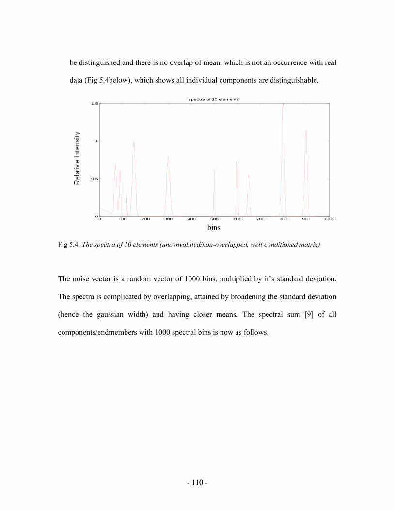
- 110 - 110

be distinguished and there is no overlap of mean, which is not an occurrence with real

data (Fig 5.4below), which shows all individual components are distinguishable.

0 100 200 300 400 500 600 700 800 900 10000

0.5

1

1.5spectra of 10 elements

Fig 5.4: The spectra of 10 elements (unconvoluted/non-overlapped, well conditioned matrix)

The noise vector is a random vector of 1000 bins, multiplied by it’s standard deviation.

The spectra is complicated by overlapping, attained by broadening the standard deviation

(hence the gaussian width) and having closer means. The spectral sum [9] of all

components/endmembers with 1000 spectral bins is now as follows.

bins

- 111 - 111

5.4.1 SVD with Generalized Inverse Methods

The Reflectance matrix (R) is composed of all individual spectra which is studied using

generalized inverse methods [12] and principal component analysis [46, 47] to find the

weight vector or the vector comprising the different compositions w. The starting

equation is as follows.

η+= wRS *r

----- (5.1)

The problem is essentially to find the estimated value to the composition vector, w. The

least squared error (LSE) [45] between the estimated and true composition vector can be

then studied to make a precise detection of the early symptoms of ARMD. The least

Fig-5.5a: The simulated spectra of macular pigment showing a highly ill-conditioned matrix with a condition 106, on which the theory of spectral unmixing is applied.

Fig-5.5b: Absorption spectrum for the Xanthophyl protein that comprises the macular degeneration peaks 459 nm. The data points for peri-macular and foveal area are averaged over five eyes.

wavelength

- 112 - 112

square error can be studied with alteration of the noise variance. Since the Reflectance

matrix [9] is ill-conditioned, we apply regularization techniques to find out the estimated

vector.

sr is the spectrum from a known library

ℜ is a non-square matrix

wr is the weight vector

ηr

is the noise vector

A pseudo-inverse or pinv (Moore-Penrose Pseudo inverse technique) is performed on the

Reflectance matrix to find the inverse matrix of this non square matrix of dimensions

1000*10. A Singular Value Decomposition is carried out (SVD) [9] to factorize the

reflectance matrix into a right (V)and left (U) singular matrices which are ortho-normal

to each other, such that:

TVUR Σ= , TT RRRR 11 )( −− = --- (5.2)

where, Σ is a diagonal matrix containing the eigen values,

So, Σ= Diag(si).

This is the reason SVD acts in such an advantageous way, where a non-square matrix can

be easily decomposed into products of two column orthogonal matrices and a diagonal

matrix. Since the original matrix is now decomposed into product of three orthonormal

- 113 - 113

matrices, inversion of the spectral reflectance matrix R is done by simply taking

transposes and reciprocal values.

When a generalized Inverse Transform is performed, we obtain:

)4.5(,

)3.5()(

11

1

1

1

111

→===

→=Σ=

−

−−

−−−

sscs

UsVdiagUVR

nni

Ti

T

ννν

Applying the inverse matrix on the known data (spectral image), we obtain:

)5.5()(*)( 11 →== −− SUsVdiagSRpinvSR Ti

r

‘c’ is the condition number of the inverse matrix, also defined as the ratio of the largest to

the smallest eigen value in the reflectance matrix. It is large (~ 100 ), which makes the

problem ill-conditioned. The instability attained by multiplying the singular matrices

with very small eigen values is addressed by use of filters, also resulting in a huge

amplification of the noise term. So, we resort to different regularization techniques. The

two of techniques I have applied are described below.

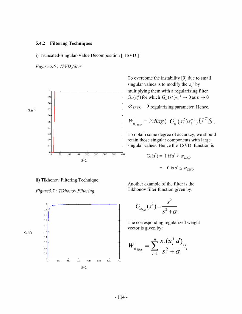
- 114 - 114

5.4.2 Filtering Techniques

i) Truncated-Singular-Value Decomposition [ TSVD ]

Figure 5.6 : TSVD filter

ii) Tikhonov Filtering Technique:

Figure5.7 : Tikhonov Filtering

To overcome the instability [9] due to small singular values is to modify the 1−

is by multiplying them with a regularizing filter Gα )( 2

is for which 0)( 12 →−ii ssGα as s 0→

→TSVDα regularizing parameter. Hence,

(VdiagWTSVD

=α 12 )( −

ii ssGα ) SU T.

To obtain some degree of accuracy, we should retain those singular components with large singular values. Hence the TSVD function is

Gα(s2) = 1 if s2 > TSVDα

= 0 is s2 ≤ TSVDα

Another example of the filter is the Tikhonov filter function given by:

αα += 2

22)(

sssG

Tikh

The corresponding regularized weight vector is given by:

i

n

i i

Tii v

sdus

WTikh ∑

= +=

12

)(αα

Gα(s2)

Gα(s2)

S^2

S^2

- 115 - 115

5.4.3 Error Estimation

The original constituent concentration vector [9], also referred as the weight vector is w.

The estimated concentration vector is w’.

The mean estimated error is: )6.5()'(1 2 →−∑ ii

i wwn

Error Estimation Chart

Estimated Weight Vector :– sR 1−

Error :

True Weight Vector =

=wr

Ar

mean squared error (MSE) :-

Least Mean Squared error =

)(1

i

n

ii wAe −= ∑

=

( )( )Ti

ii wAwA)w(Ae −− =−=Σ= ∑ 22^

0=∂

∑∂w

Minimizing the mean squared error brings us back to the starting criterion of the Moore

Penrose Inverse method. The error as described in the chart above is evaluated and

recorded in the table 5.1 below. To introduce more noise and to bring about more

instability to this inverse problem, we make the means more closer and vary the means,

standard deviations and weights to obtain different reflectance matrices with different

condition numbers. Each set of simulation for different simulated Reflectance matrices

is considered for 2 different sets of random noise changing the regularization parameters

of the filters. The errors without any regularization (error 1), error with TSVD (error 2)

and error with Tikhonov filter (error 3) are shown below in table 5.1

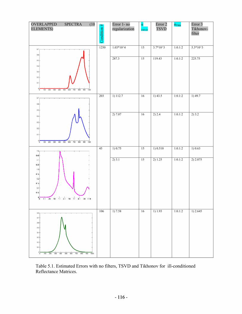
- 116 - 116

Table 5.1. Estimated Errors with no filters, TSVD and Tikhonov for ill-conditioned Reflectance Matrices.

OVERLAPPED SPECTRA (10 ELEMENTS)

Con

ditio

n # Error 1- no

regularization α TSVD

Error 2 TSVD

αTikh Error 3 Tikhonov-filter

1250 1.03*10^4

15 3.7*10^3

1:0.1:2 5.3*10^3

287.3 15 119.43 1:0.1:2 225.75

203 1) 112.7

16 1) 43.5

1:0.1:2 1) 49.7

2) 7.07 16 2) 2.4 1:0.1:2 2) 3.2

45 1) 0.75

15 1) 0.510

1:0.1:2 1) 0.63

2) 3.1 15 2) 1.25 1:0.1:2 2) 2.075

106 1) 7.58

16 1) 1.93

1:0.1:2 1) 2.645

- 117 - 117

The Inverse problem is described for different sets of data having different condition

numbers. When problem is heavily ill-conditioned, like in the first case the error is

amplified hugely. With lower condition numbers the error decreases, but cannot be

considered to be negligible. My attempt is to use statistical methods to minimize the

mean squared error for early recognition of the macular pigment. The Truncated SVD

filter with different regularization parameters generates lesser error than the Tikhonov for

these sets of simulated Reflectance data. So, I concluded the TSVD filter yields better

results in this case. But before finding out the weight vector which yields minimum error,

we have to decide on an eigen value threshold or in other words which eigen vectors from

the covariance matrix based on the target matrix has the highest effects. This is achieved

by Principal Component Analysis, which is necessary to reduce the noise by eliminating

the secondary eigen values.

5.5 Principal Component Analysis Techniques

The covariance matrix K corresponding to the Reflectance matrix R is quadratic and

symmetric and can be diagonalized by finding a matrix Q such that

λ=− KQQ 1, where λ’s are the eigen values ----- (5.7)

PCA allows data compression to reduce the dimensionality [9, 45, 12] of huge data sets

and also is a good answer to eliminate the multicolinearity problems existing between the

different spectral profiles combined to form the reflectance matrix R. The eigen vector

- 118 - 118

corresponding to each eigen value are calculated. The next step is to order them by eigen

value, highest to lowest. This gives us the components in order of significance. Now we

can decide to ignore the components of lesser significance and filter out noise. Principal

component analysis treats noise in a way that noise increases with the increasing number

of principal axes. For this purpose, Malinowski [9] grouped the eigen values into two

groups such that the primary eigen values consist of the true spectral features or the

variances and the secondary eigen values actually gives us an idea of the experimental

noise factor.

∑∑∑+===

+=m

pjj

p

jj

m

jj

1

0

1

1

1λλλ ------ (5.8)

The first denotes the primary eigen values, which contain the most significant principal

components, whereas the second term contains the less significant eigen values, which

basically incorporates to the noise factor and the real experimental error can be measured

by the second term in the equation. What needs to be done now is to form a feature

vector [46], constructed by taking the eigenvectors that we want to keep from the list of

eigenvectors, and forming a matrix with these eigenvectors in the columns. Once we have

chosen the components (eigenvectors) that we wish to keep in our data and formed a

feature vector, we simply take the transpose of the vector and multiply it on the left of the

original data set, transposed. Final Data= Row Feature Vector * Row data Adjust. This

will give us the original data-set in terms are the vital eigen vectors we chose with the

vectors which affect the variance of the original data set (R) the most.

- 119 - 119

Hence the following are achieved by using principal component analysis method. We can

easily place a threshold on the eigen value and thus lessen the dimensionality and in turn

the noise effects creating the high condition number or the instability in the inverse

problem.

- 120 - 120

5.6 Detection Techniques using Receiver Operating Curves

To verify the credibility of the detection results, graphs of detection probability are

plotted called the receiver operating curves [19] or more popularly known as ROCs

shown in Fig 5.8. These will be used to find the probability of detection PD or sensitivity

and probability of false alarm or PFA for any given correlation threshold in the findings

once the de-oxygenated cells are recognized. This is an accurate way of establishing the

accuracy and credibility of the macular degeneration hyperspectral analysis and the ROC

analysis is widely utilized in medical imaging research. The probability of detection may

be represented as a function of several independent attributes like the correlation

moments described by Physically Motivated Correlation Formalism (PMCF), Spectral

angle mapper (SAM), adaptive cosine estimator (ACE) [20] etc. So, the total probability

will be product of each probability. The analysis will not be too erroneous if each of the

probabilities is considered separately for detection and false alarm probabilities.

This image shows an area in the retina infected with macular degeneration marked with

blue outlines, also referred to as the regions of interest or ROIs and the graph shows

ROCs based on parameters like PMCF and SAM. ROCs based on these measures will

prove to be extremely handy tools for ophthalmologists and one can easily speculate.

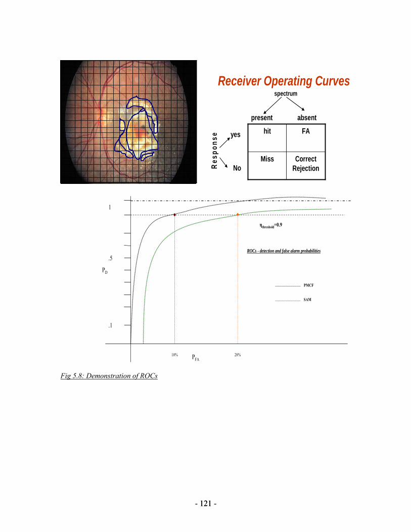
- 121 - 121

Receiver Operating Curves

Correct Rejection

Miss

FAhit

spectrum

present absent

Res

pons

e yes

No

.5

.1

10% 28%

ηthreshold=0.9

PD

ROCs - detection and false alarm probabilities

SAM

PMCF

1

PFA

Fig 5.8: Demonstration of ROCs

- 122 - 122

Some terms in determining ROCs

ηN = Number of pixels within the chosen ROIs infected with the ARMD

corresponding to the chosen threshold value η, which may be the PMCF/SAM/ACE

coefficient = probability of detection PD at that threshold.

'ηN = Number of pixels outside the chosen ROIs corresponding to the chosen threshold

value η = Probability of False Alarm (PFA) at that threshold.

The following chapter discusses in details about the results from the generated after

exploiting the clinical data on macular degeneration from Kestrel Corp. The expected end

results are as follows, which will be established in the next chapter.

1. Complete spectral analysis of the de-oxygenated cells

2. Locate the hyper-pigmentation ROIs and Spectral matching

3. Measure detection probabilities with ROCs for precision

- 123 - 123

4. Early Recognition of ARMD with Spectral Unmixing Model leading to early

treatment.

5. Concluding from the above facts that HSI/Models are promising methods to

ophthalmologists for diagnosis of ARMD.

- 124 - 124

Chapter 6

6 HYPER-SPECTRAL ANALYSIS & UN-MIXING OF MACULAR

DEGENERATION PIGMENT

6.1 Introduction

Chapter 6 contains the results of hyper-spectral analysis on a target containing age related

macular degeneration (ARMD) [3]. The data for the following research has been

registered using the Kestrel’s Fundus Imager [4], which has the similar design as the

VFTHSI integrated onto a standard clinical Fundus camera. It will be useful to refer to

the MATLAB codes in the appendix for a better understanding of the results and

discussions in this chapter. The results may be sub-divided as follows:

(a)The analysis consists of spectral analysis of reflectance data from image

interferograms to find the detailed spectra of normal and deoxygenated retina,

owing to the hyper-pigmentation caused by degeneration of the macular pigment

comprised of carotenoids, Xanthophyl protein, lutein [18] and other recently

discovered components like meso- zeaxanthin.

(b) Disease detection by application of PMCF [5] by spectral mapping of target

oxygenated cells from retina of a normal subject to the retina of 3 subjects

containing MD.

- 125 - 125

(c) After sampling the data sets and detecting the infected areas with spectral

recognition, receiver operating curves (ROC) curves depicting the probability of

detection Vs the probability of false alarm of MD within chosen area of interest

are plotted.

(d) Linear spectral un-mixing using Inverse imaging methods and principal

components analysis to find out the percentage composition of the different

protein constituents (as mentioned in point[a]) present in the MD, which can be

utilized by Ophthalmologists easily for an early recognition of ARMD.

Before we begin the analysis and discuss the results, here is a little more about MD.

At the back of the eye the macula is a tiny area about 5 mm in diameter, with the fovea at

its centre. There are no blood vessels, but lots of cells full of photosensitive pigments that

allow us to see detail in the centre of vision. As people get older, the cells with retinal

pigment become less efficient, the membrane degenerates, some cells atrophy, waste

products build up, and central vision is gradually lost. That process is age-related macular

degeneration.

Age related macular degeneration (ARMD) is the leading cause of visual loss in people

over the age of 65 years in the United States. Although the pathogenesis of AMD remains

a matter of debate, there is a growing body of evidence to indicate that oxidative damage

- 126 - 126

plays a role. The yellow coloration of the macula lutea is attributable to the presence of

macular pigment in the axons of its photoreceptors. In the 1980s several investigators

demonstrated that macular pigment consists of the xanthophyll isomers, lutein [13] and

zeaxanthin. Although the role of the macular pigment remains uncertain, several

functions have been hypothesized and these include reduction of the effects of light

scatter and chromatic aberration on visual performance, limitation of the damaging photo-

oxidative effects of blue light through its absorption, and protection against the adverse

effects of photochemical reactions because of the antioxidant properties of the

carotenoids. Research in high-performance liquid chromatography (HPLC) [8] also

shows that plasma zeaxanthin was significantly associated with reduced risk of ARMD.

Among other carotenoids, only ß-carotene showed a significant negative association with

nuclear cataract, but not ARMD.

Lutein and zeaxanthin are two elements which are antioxidants and accumulate in the

macular pigmented area. Consuming these elements more will increase the percentage in

the blood level. Zeaxanthin is preferentially found in the foveal region and lutein in the

perifoveal region. A systematic review examines how these two pigments might be

related to protection against macular degeneration. Lutein and zeaxanthin may protect the

retina in two ways, as antioxidants to oxidative stress from metabolism, and, by filtering

short wavelengths of light they also reduce the oxidative effect of blue light, which is the

reason why the absorbance spectra ranges in the bluish green area.

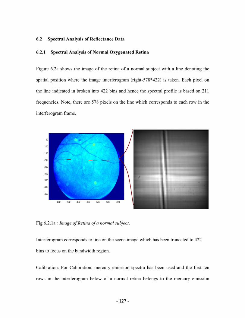
- 127 - 127

6.2 Spectral Analysis of Reflectance Data

6.2.1 Spectral Analysis of Normal Oxygenated Retina

Figure 6.2a shows the image of the retina of a normal subject with a line denoting the

spatial position where the image interferogram (right-578*422) is taken. Each pixel on

the line indicated in broken into 422 bins and hence the spectral profile is based on 211

frequencies. Note, there are 578 pixels on the line which corresponds to each row in the

interferogram frame.

100 200 300 400 500 600 700

50

100

150

200

250

300

350

400

450

Fig 6.2.1a : Image of Retina of a normal subject.

Interferogram corresponds to line on the scene image which has been truncated to 422

bins to focus on the bandwidth region.

Calibration: For Calibration, mercury emission spectra has been used and the first ten

rows in the interferogram below of a normal retina belongs to the mercury emission

- 128 - 128

interfrogram. The wavelengths taken for calibration are the highest intensities at 436, 546

and 577 nm. Table 6.2 shows Hg- I lines and is taken from the NIST [6] reference tables

and the three high intensity lines are found out from the analysis based on their ratios.

The spectra range after calibration is from 336 to 826nm. The Hg I interferogram and

spectra plotted against binning pixels and wavelengths are shown in figure 6.2b below.

Figure 6.2c shows the filtered signal interferogram and the corresponding spectrum of a

normal retina. It peaks around 540nm, where the retinal sensitivity is maximum. The

steps to compute the signal and spectrum is given below the figure.

- 129 - 129

Interferogram of a normal subject

0 50 100 150 200 2500

50

100

150Calibration with Hg emission spectra

binning pixel

Inte

nsity

400 500 600 700 8000

50

100

150 Hg emission spectra

wavelength in nm

abso

lute

Inte

nsity

Fig6.2.1b (Left) shows the interferogram of normal retina (with first 10 rows for calibration purpose). The spectra is over 211 bins which are converted to the corresponding wavelengths.

- 130 - 130

Table 6.1. Table showing the Hg–I lines from NIST reference tables and their relative intensity values. [The wavelengths taken for calibration are the highest intensities at 436, 546 and 577 nm].

Observed

Wavelength

Air (nm)

Relative

Intensity

Ei

(cm-1)

Ek

(cm-1)

Configurations Terms

404.6565 1800 37 645.080 62 350.456 5d106s(2S)6p - 5d106s(2S)7s 3P° - 3S

407.7837 150 39 412.300 63 928.243 5d106s(2S)6p - 5d106s(2S)7s 3P° - 1S

410.805 40 54 068.781 78 404.387 5d106s(2S)6p - 5d106s(2S)9s 1P° - 1S

433.922 250 54 068.781 77 107.917 5d106s(2S)6p - 5d106s(2S)7d 1P° - 3D

434.7506 400 54 068.781 77 064.097 5d106s(2S)6p - 5d106s(2S)7d 1P° - 1D

435.8335 4000 39 412.300 62 350.456 5d106s(2S)6p - 5d106s(2S)7s 3P° - 3S

488.300 5 62 350.456 82 823.94 5d106s(2S)7s - 5d106s(2S)13p 3S - 1P°

488.991 5 62 350.456 82 795.03 5d106s(2S)7s - 5d106s(2S)13p 3S - 3P°

491.607 80 54 068.781 74 404.590 5d106s(2S)6p - 5d106s(2S)8s 1P° - 1S

510.270 20 62 350.456 81 942.444 5d106s(2S)7s - 5d106s(2S)11p 3S - 1P°

512.064 40 62 350.456 81 873.835 5d106s(2S)7s - 5d106s(2S)11p 3S - 3P°

513.794 20 62 350.456 81 811.876 5d106s(2S)7s - 5d106s(2S)11p 3S - 3P°

529.074 20 63 928.243 82 823.94 5d106s(2S)7s - 5d106s(2S)13p 1S - 1P°

531.678 5 71 295.15 90 096 5d106s(2S)7p - 5d106p2 1P° - 3P

535.405 60 62 350.456 81 022.9 5d106s(2S)7s - 5d106s(2S)10p 3S - 3P°

538.463 30 62 350.456 80 916.686 5d106s(2S)7s - 5d106s(2S)10p 3S - 3P°

546.0750 1100 44 042.977 62 350.456 5d106s(2S)6p - 5d106s(2S)7s 3P° - 3S

554.963 30 63 928.243 81 942.444 5d106s(2S)7s - 5d106s(2S)11p 1S - 1P°

567.586 160 62 350.456 79 964.1 5d106s(2S)7s - 5d106s(2S)9p 3S - 1P°

576.9610 240 54 068.781 71 396.220 5d106s(2S)6p - 5d106s(2S)6d 1P° - 3D

578.966 100 54 068.781 71 336.164 5d106s(2S)6p - 5d106s(2S)6d 1P° - 3D

579.0670 280 54 068.781 71 333.182 5d106s(2S)6p - 5d106s(2S)6d 1P° - 1D

580.378 140 63 928.243 81 153.614 5d106s(2S)7s - 5d106s(2S)10p 1S - 1P°

- 131 - 131

0 50 100 150 200 250 300 350 400 450-150

-100

-50

0

50

100Signal Interferogram from Retina of normal subject

pix

Inte

nsity

400 500 600 700 800 900 10000

200

400

600

Spectrum of normal fovea

wavelength nm

Inte

nsity

Figure 6.2.1c Filtered signal interferogram and the corresponding spectrum of a normal

retina (row 196).

Spectral Analysis Steps:

1. Plotting the signal Interferogram.

1.1. The signal data X is fitted into a polynomial fit to a degree n using least

squared estimates. The number of binning pixels are n+1, so that we obtain

- 132 - 132

polynomial coefficients in descending powers :P(1)*X^N + P(2)*X^(N-1) +...+

P(N)*X + P(N+1).

1.2 The error estimates are then calculated for predictions by using the

function Polyval in Matlab. An output structure S is used to obtain error estimates

for predictions, which contains fields for the triangular factor (R). R is a triangular

matrix generated from a QR decomposition [12]of the Vandermonde matrix of the

original signal vector X . If the degrees of freedom is denoted by f and the norm of

the residuals by rnorm, and assuming the data in the output signal vector Y is

random, an estimate of the covariance matrix of P is given by : [ ]Tnorm RRf

r 112

* −−

1.3 A filter vector with the same size as the signal vector is created by a

polynomial fit of the estimated errors, which is subtracted from the signal to obtain

the filtered signal.

2. Plotting the spectrum:

2.1 The calibration is used to convert from pix to wavelength mapping.

2.2 A fast Fourier transform is applied to the filtered signal to obtain the spectral

profile (say y).

2.3 The spectrum ( yyT ) is plotted against the wavelength.

- 133 - 133

6.2.2 Analysis for the Macular Degeneration spectral Profile

100 200 300 400 500 600 700

50

100

150

200

250

300

350

400

450

Fig 6.2.2a (Left): The Interferogram (636rows*453cols) frame of a subject with macular degeneration. The spatial extent/dimension and location at which this interferogram is taken has been indicated by the line drawn on the 2D scene image (below). The macular pigment can easily be detected towards the right edge which corresponds to the abnormal spectra. The line has 663 pixels (ends chopped to give just 636 pixels) which are smeared into 453 binning wavelengths.

- 134 - 134

Fig 6.2.2b Interferogram showing Hg emssion

- 135 - 135

Picture 6.2.2b above shows the presence of Hg emission spectra for calibration around

row 648. This interferogram belonging to subject ‘B’ (dimension: 679*427) containing

the macular degeneration pigment was truncated from it’s initial dimensions to obtain the

area of interest for this analysis.

0 50 100 150 200 250 300 350 400 450-3

-2

-1

0

1x 104 Signal Interferogram of Hg

pix

Inte

nsity

0 50 100 150 200 2500

2

4

6x 104

X: 174Y: 1.959e+004

Calibration with Hg emission spectra

binning pixel

Inte

nsity

Fig 6.2.2c: Calibration spectra- Hg emission spectra

Pixel location wavelength Wavelength/pixel

59 436nm

112 546nm 2.07nm

174 579nm 1.87nm

Average wavelength /pixel -2nm

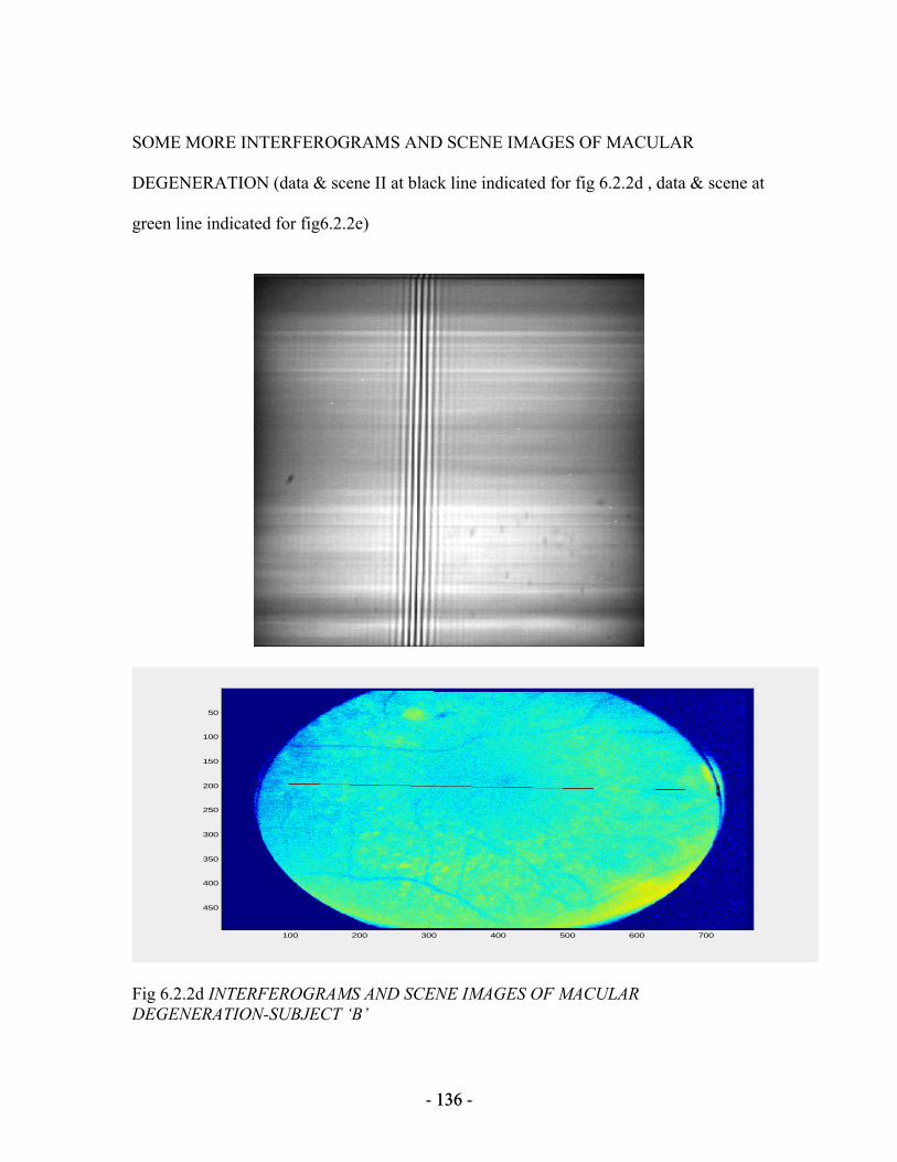
- 136 - 136

SOME MORE INTERFEROGRAMS AND SCENE IMAGES OF MACULAR

DEGENERATION (data & scene II at black line indicated for fig 6.2.2d , data & scene at

green line indicated for fig6.2.2e)

100 200 300 400 500 600 700

50

100

150

200

250

300

350

400

450

Fig 6.2.2d INTERFEROGRAMS AND SCENE IMAGES OF MACULAR DEGENERATION-SUBJECT ‘B’

- 137 - 137

100 200 300 400 500 600 700

50

100

150

200

250

300

350

400

450

Fig 6.2.2e INTERFEROGRAMS AND SCENE IMAGES OF MACULAR DEGENERATION-SUBJECT ‘C’

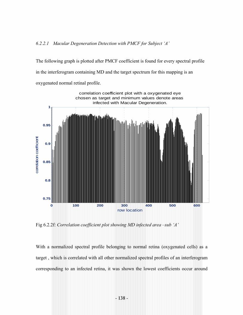
- 138 - 138

6.2.2.1 Macular Degeneration Detection with PMCF for Subject ‘A’

The following graph is plotted after PMCF coefficient is found for every spectral profile

in the interferogram containing MD and the target spectrum for this mapping is an

oxygenated normal retinal profile.

0 100 200 300 400 500 600

0.75

0.8

0.85

0.9

0.95

1

row location

corre

latio

n co

effic

ient

correlation coefficient plot with a oxygenated eyechosen as target and minimum values denote areas

infected with Macular Degeneration.

Fig 6.2.2f: Correlation coefficient plot showing MD infected area –sub ‘A’

With a normalized spectral profile belonging to normal retina (oxygenated cells) as a

target , which is correlated with all other normalized spectral profiles of an interferogram

corresponding to an infected retina, it was shown the lowest coefficients occur around

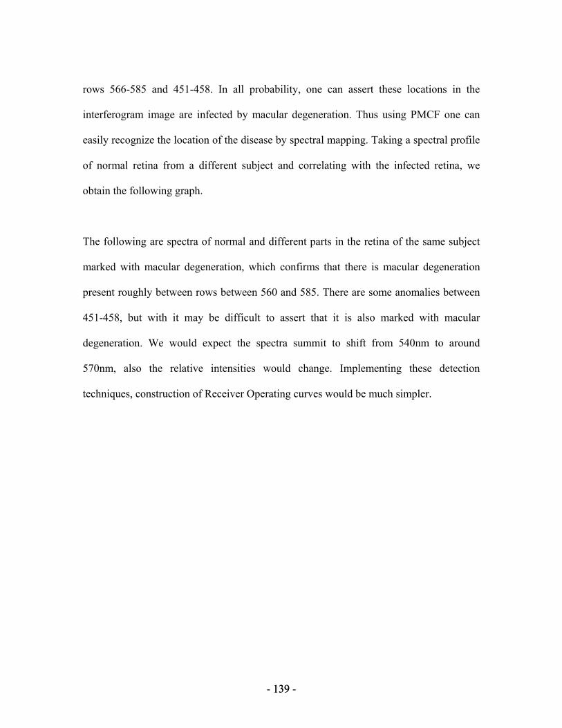
- 139 - 139

rows 566-585 and 451-458. In all probability, one can assert these locations in the

interferogram image are infected by macular degeneration. Thus using PMCF one can

easily recognize the location of the disease by spectral mapping. Taking a spectral profile

of normal retina from a different subject and correlating with the infected retina, we

obtain the following graph.

The following are spectra of normal and different parts in the retina of the same subject

marked with macular degeneration, which confirms that there is macular degeneration

present roughly between rows between 560 and 585. There are some anomalies between

451-458, but with it may be difficult to assert that it is also marked with macular

degeneration. We would expect the spectra summit to shift from 540nm to around

570nm, also the relative intensities would change. Implementing these detection

techniques, construction of Receiver Operating curves would be much simpler.

- 140 - 140

Fig 6.2.2g: Mesh plot of all spectral profiles in the infected retina- subject ‘A’

MD region for subject A

- 141 - 141

The normal profile used as a target for the above figure belongs to the target (normal eye

–row 372).

Below is a plot of PMCF coefficients and row location to recognize areas infected with

macular degeneration. The standard error (standard deviation/ √n) is also shown on the

plot, where n denotes the number of observations or in other words the number of pixels

on the line drawn on fig 6.2.2h indicating the spatial extent of the slit. The standard

deviation is 0.0476 and the standard error is 0.0001, which proves the detection accuracy

is high.

0 100 200 300 400 500 6000

0.05

0.1

0.15

0.2

0.25

0.3

0.35

0.4

ROW LOCATION

PM

CF

CO

EFF

ICIE

NT

PMCF COEFFICIENTS SHOWING PRESENCE OF MACULAR DEGENERATION AOI AROUND ROWS 566-585 WITH HIGH DISEASE DETECTION PROBABILITY

- 142 - 142

Fig 6.2.2h: PMCF coefficients showing MD

We chose an AOI, which demonstrates the highest possibility of macular pigment

infection presence and find the probability of detection of macular degeneration within

the area Vs the probability the probability of false alarm using ROCs.

6.2.2.2 Detection Techniques using Receiver Operating Curves for subject ‘A’

Model Outline:

A={ the macular pigment is present}

B= {PMCF coefficient registers the presence of macular degeneration}

Ac= {macular pigment is not present}

Bc ={PMCF coefficient does not register the presence of macular degeneration}

Probability of detection = )()()( ABPAPBAP =∩

The probability is calculated as the number of pixels within the chosen ROIs infected

with the ARMD corresponding to the chosen threshold value η, which may be the

PMCF/SAM/ACE coefficient = probability of detection PD at that threshold. This value is

denoted by ηN .

Probability of False Alarm = )()()( ccc ABPAPBAP =∩

- 143 - 143

The probability of false alarm would be the number of pixels outside the chosen ROIs

corresponding to the chosen threshold value η, which is the PMCF coefficient =

Probability of False Alarm (PFA) at that threshold and is denoted by 'ηN .

- 144 - 144

Fig 6.2.2i: Histogram plots for detection probability and false alarm

0.24 0.26 0.28 0.3 0.32 0.34 0.36 0.380

1

2

3

4Histogram of AOI with macular degeneration-Detection probability

PMCF coefficients

no. o

f pix

0 0.05 0.1 0.15 0.2 0.25 0.3 0.350

50

100

150Histogram of the area outside AOI-False alarm

PMCF coefficients

no. o

f pix

The following roc curves belong to the abnormal image – I as shown in figure 6.2.2j with

the area of interest (AOI) chosen is the area on by fig 6.2.2g indicated to have the

macular degeneration pigment. The probabilities of MD disease detection and false alarm

are dependent on the PMCF coefficients plotted on the secondary axis in fig 6.2.2j. The

detection probability corresponding a particular coefficient is given by the normalized

ratio of number of the pixels within the chosen AOI which generates that particular

coefficient to that of the total number of pixels in the AOI. The probability of false alarm

- 145 - 145

corresponding to a particular coefficient is given by the normalized ratio of the pixels

outside the chosen AOI to that of the total number of pixels save the pixels in the AOI.

ROC curve for MD detection

y = 2.1299x2 - 2.7386x + 0.7193

0

0.1

0.2

0.3

0.4

0.5

0.6

0.7

0.8

0.9

1

0.00010.0010.010.11Probability of False Alarm

Prob

abili

ty o

f MD

det

ectio

n w

ithin

AO

I

0

0.05

0.1

0.15

0.2

0.25

0.3

0.35

0.4

corr

espo

ndin

f PM

CF

coef

ficie

nts

Fig 6.2.2j: ROC analysis for subject ‘A’ diagnosed with macular degeneration.

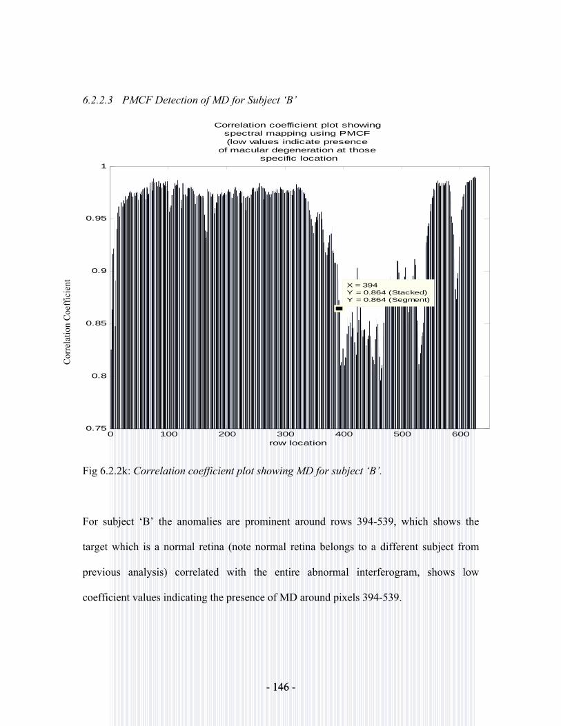
- 146 - 146

6.2.2.3 PMCF Detection of MD for Subject ‘B’

0 100 200 300 400 500 6000.75

0.8

0.85

0.9

0.95

1

X = 394Y = 0.864 (Stacked)Y = 0.864 (Segment)

Correlation coefficient plot showing spectral mapping using PMCF (low values indicate presence

of macular degeneration at those specific location

row location

Fig 6.2.2k: Correlation coefficient plot showing MD for subject ‘B’.

For subject ‘B’ the anomalies are prominent around rows 394-539, which shows the

target which is a normal retina (note normal retina belongs to a different subject from

previous analysis) correlated with the entire abnormal interferogram, shows low

coefficient values indicating the presence of MD around pixels 394-539.

Cor

rela

tion

Coe

ffic

ient

- 147 - 147

Fig 6.2.2l: Mesh plot of all spectral profiles in the infected retina –sub ‘B’.

After finding all spectral profiles of each of the 627 rows over 211 frequencies in the

interferogram frame belonging to subject ‘B’ diagnosed with macular degeneration, a 3-D

mesh plot above indicates a region where the MD pigment spectra can be easily

recognized. The spectra is studied in details below.

MD region

Noise Normal region

- 148 - 148

6.2.2.4 Plotting spectra of Macular Degeneration from different parts of the interferogram

Our wavelength range of interest is from 400 -600 nm. There are features beyond the

range, but this does not contribute to the pigment spectra, hence it is truncated from the

spectral graphs as shown below.

Fig 6.2.2 m: Macular Degeneration Pigment spectra at different parts of AOI.

450 480 510 540 570 600 630 6500

0.1

0.2

0.3

0.4

wavelength in nm

Inte

nsity

MD spectrum-row 395

450 480 510 540 570 600 630 6500

0.1

0.2

0.3

0.4

0.5

wavelength in nm

Inte

nsity

MD spectrum-row 400

450 480 510 540 570 600 630 6500

0.1

0.2

0.3

0.4

wavelength in nm

Inte

nsity

MD spectrum-row 410

450 480 510 540 570 600 630 6500

0.1

0.2

0.3

0.4

wavelength in nm

Inte

nsity

MD spectrum-row 465

450 480 510 540 570 600 630 6500

0.1

0.2

0.3

0.4

0.5

wavelength in nm

Inte

nsity

MD spectrum-row 532

470 500 530 560 590 620 6500

0.05

0.1

0.15

0.2

0.25

0.3

0.35

wavelength in nm

Inte

nsity

MD spectrum-row 454

- 149 - 149

460 480 500 520 540 560 580 600 620 640 6500

0.05

0.1

0.15

0.2

0.25

0.3

0.35

X: 558Y: 0.3376

wavelength in nm

Inte

nsity

MD spectrum

Fig 6.2.2 n: MD Spectrum – known spectral library in the inverse problem.

Thus the graph of the macular pigment above shows it to peak around 558-560 nm

corresponding to row 454 in the interferogram image frame, which indicates a

wavelength shift towards the yellow region of the visible spectra and can be explained by

the yellow nature of this pigmentation. This data is taken as the known spectral library in

the following section where inverse imaging techniques are involved to compute the

percentage composition of the constituents in the macular pigment.

- 150 - 150

100 200 300 400 500 6000

0.05

0.1

0.15

0.2

0.25

row location

PM

CF

coef

ficen

terrorbar plot of PMCF coefficients to

find the area with maximum MD detection probability (rows 394:540)

Fig 6.2.2 o: Error-bar plot of PMCF coefficients showing MD

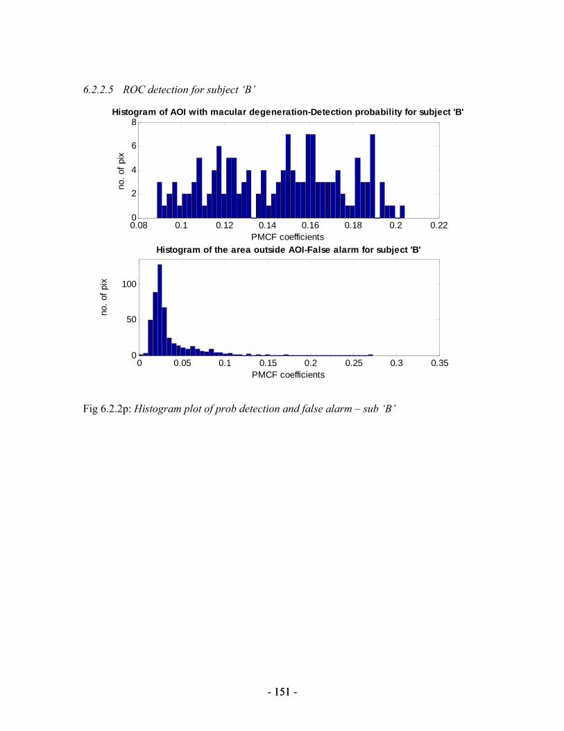
- 151 - 151

6.2.2.5 ROC detection for subject ‘B’

0.08 0.1 0.12 0.14 0.16 0.18 0.2 0.220

2

4

6

8Histogram of AOI with macular degeneration-Detection probability for subject 'B'

PMCF coefficients

no. o

f pix

0 0.05 0.1 0.15 0.2 0.25 0.3 0.350

50

100

Histogram of the area outside AOI-False alarm for subject 'B'

PMCF coefficients

no. o

f pix

Fig 6.2.2p: Histogram plot of prob detection and false alarm – sub ‘B’

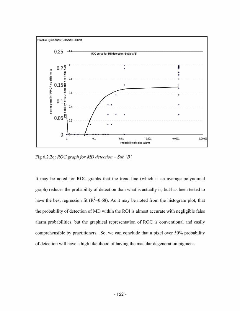
- 152 - 152

ROC curve for MD detection -Subject 'B'

trendline : y = 3.1629x2 - 3.5279x + 0.6291

0

0.2

0.4

0.6

0.8

1

1.2

0.000010.00010.0010.010.11Probability of False Alarm

Prob

abili

ty o

f MD

det

ectio

n w

ithin

AO

I

0

0.05

0.1

0.15

0.2

0.25co

rres

pond

inf P

MC

F co

effic

ient

s

Fig 6.2.2q: ROC graph for MD detection – Sub ‘B’.

It may be noted for ROC graphs that the trend-line (which is an average polynomial

graph) reduces the probability of detection than what is actually is, but has been tested to

have the best regression fit (R2=0.68). As it may be noted from the histogram plot, that

the probability of detection of MD within the ROI is almost accurate with negligible false

alarm probabilities, but the graphical representation of ROC is conventional and easily

comprehensible by practitioners. So, we can conclude that a pixel over 50% probability

of detection will have a high likelihood of having the macular degeneration pigment.

- 153 - 153

6.2.2.6 ROC for subject ‘B’ based on Spectral Angle Mapper

Consider a scatter plot of pixel values from two bands of a spectral image. In such a plot,

pixel spectra and target spectra will plot as points (Fig 6.2.2r). If a vector is drawn from

the origin through each point, the angle between any two vectors constitutes the spectral

angle between those two points. The Spectral Angle Mapper (Yuhas et al., 1992)

computes a spectral angle between each pixel spectrum and each target spectrum. The

smaller the spectral angle more will be similar the pixel and target spectra. This spectral

angle will be relatively insensitive to changes in pixel illumination because increasing or

decreasing illumination doesn’t change the direction of the vector, only its magnitude.

The actual spectral angle calculation is based on all of the bands in the image as

calculated and plotted below in a histogram plot and a spectral “hyper-angle” is

calculated between each spectral profile from the interferogram containing MD target and

reference ( an average normal spectra). The higher the angular value, lower will be the

correlation between the target and the reference spectral signatures.

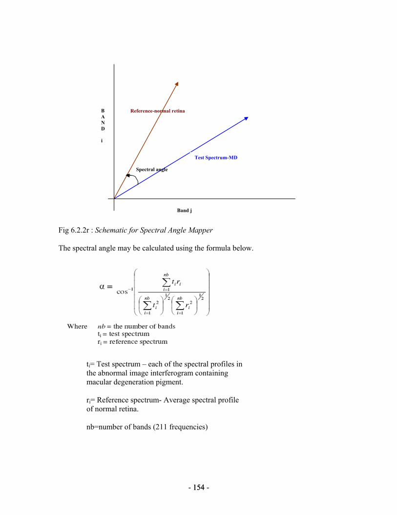
- 154 - 154

Fig 6.2.2r : Schematic for Spectral Angle Mapper

The spectral angle may be calculated using the formula below.

Test Spectrum-MD

Reference-normal retina

Spectral angle

B A N D i

Band j

ti= Test spectrum – each of the spectral profiles in the abnormal image interferogram containing macular degeneration pigment. ri= Reference spectrum- Average spectral profile of normal retina. nb=number of bands (211 frequencies)

- 155 - 155

100 200 300 400 500 600 7000.1

0.2

0.3

0.4

0.5

0.6

0.7

0.8

X: 537Y: 0.5393

row location

Spe

ctra

l ang

le

Graph of Spectral Angle Mapper to detect MD- Subject 'B'[The macular degeneration ROI lies from 395-537.]

Fig 6.2.2s: Plot of SAM coefficient in detecting MD cells for Subject ‘B’

Target is a normal retinal cell spectrally mapped with MD pigment. The high spectral

angles indicate maximum deviation from normalcy or in other words presence of macular

degeneration.

- 156 - 156

0.4 0.45 0.5 0.55 0.6 0.650

2

4

6Histogram of AOI with macular degeneration-Detection probability with SAM

SAM coefficients

no. o

f pix

0 0.05 0.1 0.15 0.2 0.25 0.3 0.350

20

40

60

80Histogram of the area outside AOI-False alarm

SAM coefficients

no. o

f pix

Fig 6.2.2t: Histogram plot of pro detection and false alarm using SAM

From the graphs above, it is very evident that there is no overlap of the SAM values in

the area where MD is detected and false alarm values outside the AOI, Hence Roc curves

may not be so meaningful to plot with this data. Nevertheless, To highlight the better

performance of PMCF algorithm as a better and precise detection tool, below if the ROC

graph for subject ‘B’ using Spectral Angle Mapper, which indicates a 50% detection

probability with negligible false alarm. It may be concluded that subject ‘A’ may have a

matured stage of MD than subject ‘B’ as evident form the higher probability detection

values with PMCF for A and it may be noted that though ‘B’ has lower percentage of

- 157 - 157

degenerated carotenoids depicting an earlier stage of ARMD, SAM fails to capture the

details showing a much lower probability of detection as compared to PMCF.

ROC curve for MD detection w.r.t SAM for subject 'B'

Statistical Fit Equation: y = 2.5441x2 - 2.8554x + 0.4392

0

0.1

0.2

0.3

0.4

0.5

0.6

0.7

0.8

0.9

1

0.00010.0010.010.11Probability of False Alarm

Prob

abili

ty o

f MD

det

ectio

n w

ithin

AO

I

0

0.1

0.2

0.3

0.4

0.5

0.6

0.7

corr

espo

ndin

gSA

M c

oeff

icie

nts

Fig 6.2.2u: ROC graph using SAM for subject ‘B’

With SAM, it may not be possible to capture the minute details, which PMCF does. The

main advantages of the SAM algorithm as a classification tool is that its an easy and rapid

method for mapping the spectral similarity of image spectra to reference spectra. The

main disadvantage of this method is the spectral mixture problem with which I deal in

details in the next section of this Chapter. The most erroneous assumption made with

SAM is the supposition that endmembers chosen to classify the image represent the pure

spectra of a reference material, which is definitely not the case. The spectral confusion in

- 158 - 158

pixels can lead to underestimation and overestimation errors for a spectral class. So, in

general, I conclude PMCF is a better classifier for the recognition of a retinal disease like

MD.

6.3 Linear Spectral Unmixing Problem of MD using Inverse Techniques

Age-related macular degeneration (ARMD) is a disease with multiple risk factors, many

of which appear to involve oxidative stress. Macular pigment, with its antioxidant and

light-screening properties, is thought to be protective against ARMD. A result has been

the appearance of dietary supplements containing the macular carotenoids, lutein and

zeaxanthin. More recently, a supplement has been marketed containing, in addition, the

third major carotenoid of the macular pigment, meso-zeaxanthin [8]. The purpose of the

study was to determine the effectiveness of such a supplement in raising macular pigment

density in human subjects.

Current evidence demonstrates that the carotenoids lutein, zeaxanthin and meso-

zeaxanthin are readily bioavailable and if supplemented will effectively increase macular

pigment levels. Nowhere in the human body is the nutritional significance of carot-enoids

more evident than in the retina. Here, at the centre of the retina (the ‘fovea’), dietary

xanthophylls are accumulated, constituting the macular pigments or macula lutea.

These yellow compounds are concentrated to the greatest extent within the inner retinal

layers so that blue light, focused upon the fovea by the lens and cornea, is filtered and

- 159 - 159

attenuated before reaching the critically functional photoreceptor and retinal pigment

epithelium layers in the outer retina. The concentration of these yellow carotenoids found

in the macular region of the retina in the eye is about 10,000 times greater than that found

in blood, attesting to a mechanism of active accumulation by this tissue. The carotenoids

of the macular pigment are classified as xanthophylls and are structurally related to

alpha- and beta-carotene; they differ from these carotenes only by the presence of

hydroxyl groups. It is startling that the retina accumulates only the xanthophylls lutein

and zeaxanthin, two of about a dozen abundant carotenoids found in the blood, while not

even traces of the other carotenoids are found in this tissue.

Lutein [8] and zeaxanthin [8] each exist in a number of different isomeric forms in

nature. This is because of the structural variability in the three-dimensional geometry of

covalently bonded carbon atoms. In addition to the ‘bent’ or cis-carotenoids that result

from the two possible arrangements of each double bond in the polyene chain, the

presence of the oxygen atoms on the end groups in the molecules also confers the

opportunity for stereoisomerism due to the handedness or chiral nature of the tetrahedral

carbon. Because of the specificity of the carotenoid biosynthetic pathways in higher

plants, the diet of humans is almost devoid of all but two stereoisomers of lutein and

zeaxanthin. Other isomers in most human food sources are present in very low quantities.

The presence of the zeaxanthin isomer, meso-zeaxanthin [18], in a high percentage in the

macular pigment, is an unexpected and interesting scientific mystery.

- 160 - 160

6.3.1 Reconstruction of spectral profiles of different end-members of macular

pigmentation from reference literature

To assess the associations of plasma lutein and zeaxanthin and other carotenoids with the

risk of age-related maculopathy (ARMD) is the final analysis of this chapter. Later, based

on the interferogram results and these experimental procedures from literature survey a

statistical model has been generated to easily asses the percentage composition of the

different components (mentioned above and in table 6.2) present in the age related

macular degeneration pigment. The table 6.2 discusses about the components which are

more evidently present and their spectral information given by the reflectance profile. All

the spectra simulated are from known profiles from references. Degeneration of these

components result in ARMD and the percentage composition of the degenerated

pigments to assert ARMD is computed in the next section.

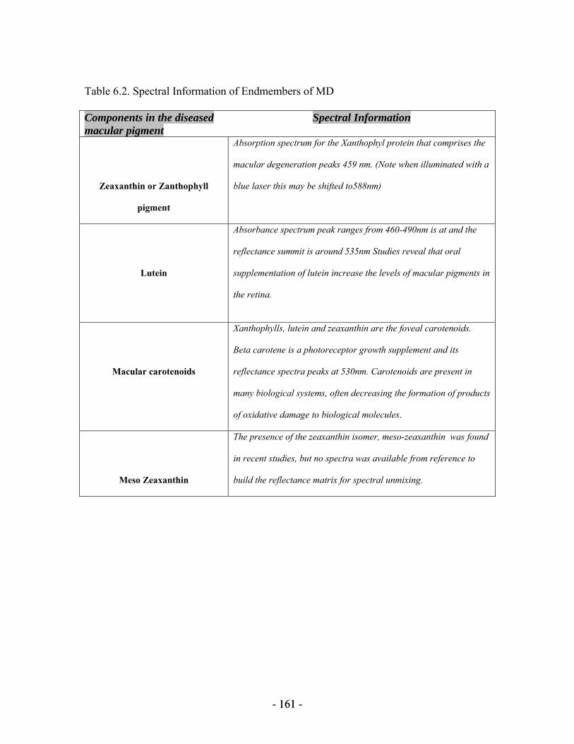
- 161 - 161

Table 6.2. Spectral Information of Endmembers of MD Components in the diseased macular pigment

Spectral Information

Zeaxanthin or Zanthophyll

pigment

Absorption spectrum for the Xanthophyl protein that comprises the

macular degeneration peaks 459 nm. (Note when illuminated with a

blue laser this may be shifted to588nm)

Lutein

Absorbance spectrum peak ranges from 460-490nm is at and the

reflectance summit is around 535nm Studies reveal that oral

supplementation of lutein increase the levels of macular pigments in

the retina.

Macular carotenoids

Xanthophylls, lutein and zeaxanthin are the foveal carotenoids.

Beta carotene is a photoreceptor growth supplement and its

reflectance spectra peaks at 530nm. Carotenoids are present in

many biological systems, often decreasing the formation of products

of oxidative damage to biological molecules.

Meso Zeaxanthin

The presence of the zeaxanthin isomer, meso-zeaxanthin was found

in recent studies, but no spectra was available from reference to

build the reflectance matrix for spectral unmixing.

- 162 - 162

Building the Reflectance matrix from reference component spectra

The following are details from literature references about building the reflection matrix R

containing the information about the individual diseased components. The reference

spectra is generally the absorbance spectra which can converted through it’s reciprocal to

find the reflectivity.

r=1-a, where r =coefficient of reflectance and a=coefficient of absorbance.

a) The Xanthophyl spectra:

The central most area of the fovea has a high absorbance for the blue-green light showing

the absorption spectrum of the Xanthophyl [7] protein of the macular pigment, which

changes rapidly in this region of the spectrum. Melanin which also absorbs blue light

does not show any rapid change in absorption in this region of the spectrum but has a

monotonic increase from the long to the short wavelengths. The reference spectra of the

Xanthophyl pigment was re-constructed as shown from the figure below. Hemoglobin is

scare in the diseased foveal area, which will generate other pigments with this

Xanthophyl protein spectrum. Hemoglobin absorbs little light at 633nm. There is also

evidence of additional pigmentation at the macula which absorbs red light , which

demonstrate there is a higher chance of this being melanin rather than hemoglobin

because hemoglobin absorbs very little red light. Fig 6.3a shows the reference absorbance

spectra for xanthophyl pigment taken at the fovea and perimacular area (13.4 deg from

the fovea). Each data point represents five eyes of three normal subjects. The maximum

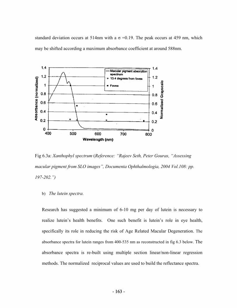
- 163 - 163

standard deviation occurs at 514nm with a σ =0.19. The peak occurs at 459 nm, which

may be shifted according a maximum absorbance coefficient at around 588nm.

Fig 6.3a: Xanthophyl spectrum (Reference: “Rajeev Seth, Peter Gouras, “Assessing

macular pigment from SLO images”, Documenta Ophthalmologia, 2004 Vol.108: pp.

197-202.”)

b) The lutein spectra.

Research has suggested a minimum of 6-10 mg per day of lutein is necessary to

realize lutein’s health benefits. One such benefit is lutein’s role in eye health,

specifically its role in reducing the risk of Age Related Macular Degeneration. The

absorbance spectra for lutein ranges from 400-535 nm as reconstructed in fig 6.3 below. The

absorbance spectra is re-built using multiple section linear/non-linear regression

methods. The normalized reciprocal values are used to build the reflectance spectra.

- 164 - 164

Fig 6.3b: Lutein absorbance spectra

Lutein absorbance spectra

0

0.2

0.4

0.6

0.8

1

1.2

401 411 421 431 441 451 461 471 481 491 501 511 521 531 541

wavelength(nm)

Nor

mal

ised

Abs

orba

nce

Fig 6.3c: UV-VIS spectra of some selected carotenoids

- 165 - 165

The figure 6.3c above shows absorbance spectra of different carotenoids, which has been

used as source for re-construction.All samples were dissolved in DMSO: 500 μM (blue

line) and 8.4 μM (turquoise line) lutein esters; 16.7 μM (orange line) β-carotene; 16.7 μM

(green line) lutein; 16.7 μM (red line) lycopene; 16.7 μM (purple line) zeaxanthin; 25 μM

(brown line) soy carotenoids. The inset shows the UV-VIS spectrum of lutein esters

(mostly palmitate from marigolds) at 8.4 μM.

The macular pigments are predominantly composed of three carotenoids: lutein,

zeaxanthin, and meso-zeaxanthin. These carotenoids are concentrated and distributed in a

selective manner. The properties of these pigments are further explored along with their

methods of uptake, stabilization, and storage. The dual nature of these pigments as filters

and antioxidants are elaborated upon in relation to their protective effects upon the

macula, specifically in age-related macular degeneration. Evidence suggests that

increased levels of macular pigment are correlated with a decreased risk of age-related

macular degeneration. Many have sought to exploit this therapeutic relation. Studies

reveal that oral supplementation with lutein and zeaxanthin can increase the levels of

macular pigments in the retina.

- 166 - 166

480 500 520 540 560 580 600 620 6400

0.05

0.1

0.15

0.2

0.25

0.3

0.35

wavelength in nm

Inte

nsity

Average MD spectrum- chosen as reference spectrum for Linear Spectral Unmixing

Lutein reflectance Spectra

0

0.1

0.2

0.3

0.4

0.5

0.6

0.7

0.8

0.9

1

1.1

400 420 440 460 480 500 520 540 560 580 600wavelength

Nor

mal

ised

Inte

nsity

Fig 6.3d: Lutein Reflectance Spectrum.

- 167 - 167

Xanthophyll Reflectance Spectrum

0

0.1

0.2

0.3

0.4

0.5

0.6

0.7

0.8

0.9

1

1.1

400 420 440 460 480 500 520 540 560 580 600 620 640

wavelength (nm)

norm

alised

refle

ctan

ce in

tens

ity

Fig 6.3e: Xanthophyl pigment reflectance spectrum.

Carotenoid reflectance spectrum (beta carotenoid)

0

0.1

0.2

0.3

0.4

0.5

0.6

0.7

0.8

0.9

1

1.1

400 420 440 460 480 500 520 540 560 580 600wavelength (nm)

norm

alis

ed in

tens

ity

The meso-zeaxanthin spectra was not available from reference papers, hence it is being

excluded from the endmember list, but recent research does establish that this component

also plays a role in the degeneration of the macular pigment.

Fig 6.3f: Beta carotenoid Reflectance spectrum. Note : All spectral profiles are reconstructed from reference literature

- 168 - 168

Using inverse methods, the percentage compositions of these end-members are found out,

which reflects that in a degenerated macular cell, what percentage composition of these

decaying or degenerating end-members will assert the presence of the MD pigment in the

fovea. The predominant carotenoids of the macular pigment are lutein, zeaxanthin, and

meso-zeaxanthin. The regular distribution pattern of these carotenoids within the human

macula indicates that their deposition is actively controlled in this tissue. Increased

macular carotenoid levels result from supplementation of humans with lutein and

zeaxanthin, which reinstates the functional role for the macular pigment in protection

against light-induced retinal damage and age-related macular degeneration.

- 169 - 169

6.3.2 Results and Discussions for the Spectral Unmixing of MD

Analyzing the de-oxygenated cells, the following percentages of the degenerated

endmembers will confirm an early stage of dry macular degeneration.

With a simple inversion (same results also attained by multiple linear regression) without

the use of any filters, we obtain an unconstrained percentage coefficient as shown in the

table below. Each of the following end-members as plotted above over 65 pixels have the

following unconstrained coefficients.

Table 6.3. Percentage Compositions of MD components from Inverse Methods.

Coefficients

Standard

Error t Stat P-value

Lower

95%

Upper

95%

LUTEIN

0.1992 0.149 1.33 0.188 -0.10 0.498

XANTHOPHYL

0.1115 0.077 1.435 0.156 -0.043 0.266

OTHER

CAROTENOIDS

(β-carotene) -0.225 0.104 1.153 0.23 -0.43 -0.016

- 170 - 170

Table 6.4. Statistics.

Regression Statistics

Multiple R 0.86

R Square 0.74

Adjusted R Square 0.71

This analysis shows that Xanthophyl is the most important out of the all the carotenoids

or protein pigments with the lowest p-value or conversely the maximum t-value. In a

degenerated macula, if 11.1% of Xanthophyl and nearly 20% lutein is found, then the

subject may be diagnosed to have ARMD. In other words, one may conclude if the end-

member spectra are considered to be pure spectra of the constituent, then in a degenerated

pigment, Xanthophyl pigment would have degenerated 89.9%, while the lutein would

have decayed almost 80%. Beta-carotene is a supplement given to ARMD patients to

prevent the disease and does not occur in the eye. The spectrum coefficient is negatively

correlated to the disease spectrum and as a consequence of these findings, beta-carotene

have been dropped from the list of end-member spectra.

Standard Error 0.089

Observations 65

- 171 - 171

The problem becomes simple with only 3 end-members. Just by basic analysis, the first

two endmembers are retained which has the eigen values as shown below. The matrix R

(dimension-65*3) is composed of the columns containing these spectra. When a pseudo

inverse is applied to it, we obtain the following results as indicated in table 6.5. The

singular value decomposition process yields two important eigen values corresponding to

lutein and xanthophyl pigment. After singular value decomposition as described in

Chapter 5, we obtain the weight vector (dimensions-3*1), left singular matrix

(dimension- 65*65) and right singular matrix (dimension- 3*3). The reflectance matrix,

which is well-conditioned with a condition number of 20.28 and containing the

endmember spectra as its columns is now diagonalised using SVD and the corresponding

eigen values are found out. The eigen values corresponding to lutein and Xanthophyl

pigment are significantly large indicating these are the primary components as shown in

table 6.5 The eigen value corresponding to beta-carotene is not significant and has no

direct relationship with MD pigment.

Table 6.5. Primary Components.

CONDITION NUMBER OF THE MATRIX R 20.28

EIGEN VALUES 9.524, 1.767, 0.469

Eigen value corresponding to lutein 9.524

Eigen value corresponding to Xanthophyl 1.767

- 172 - 172

One may also deduce that probably this subject was not given the β-carotene supplement,

which should be present otherwise in a MD patient which helps restore the degeneration

of the photo-receptors. The problem becomes a 2 primary end-member case – lutein and

xanthophyl with large eigen values associated with them. With large amount of clinical

data (an entire Hypercube), one may find newer end members through spectral unmixing.

- 173 - 173

Chapter 7

7 CONCLUSIONS

7.1 Dissertation Summary

According to Benjamin Franklin, "To err is human, to repent divine, to persist devilish."

Such were my thoughts when I cruised through a year of my doctoral studies, which

seemed an episode without a finale and also took some time to repent, but I guess my

persistence was strong enough to make this research a success, whose practical

applicability now seems significant.

Hyperspectral imaging was known to be an important tool to handle complex target

recognition remote sensing problems in a simplified way. This thesis is was an attempt to

think beyond its usual applications by analyzing targets such as plasma diagnostics

during carbon nano tube growth and retinal imaging for early recognition and diagnosis

of macular degeneration. This research treats a wide range of target and proves how

beneficial HS imaging with the Visible Fourier Transform Hyperspectral Imager could be

to analyze spectra and be of considerable assistance in especially clinical or medical

imaging industries, remote-sensing, nanotechnology research industry and several others.

The correlation formalism (PMCF) as described and formulated in Chapter 3 is used as

an analytic tool in all areas, which captures greater details, hence augmenting the

accuracy of the hyperspectral analysis compared to conventional tools like Z-testing,

SAM and other statistical detection methods. The receiver operating curves in chapter 6

- 174 - 174

clearly state the accurateness of the PMCF tool. This research is also the first known

attempt to analyze hyperspectrally RF-plasma data used to grow carbon nano-tubes as

described in Chapter 4.

Recently, when the macula has been observed with monochromatic light, comparing a

blue with a long wavelength image taken with a SLO, a qualitative indication of the

density and distribution of the macular pigment was obtained, which lacks preciseness.

This piece of current research takes it to the next level of precise investigation by

correlating the microanatomy of the diseased fovea.

Using the Fundus imager from Kestrel Corp as described in Chapter 5, hyperspectral

analysis of the interferogram frames containing the diseased retinal cells with macular

degeneration was successfully conducted in Chapter 6. The region containing MD was

easily distinguishable from the spectral mesh plots over the entire band-pass area. Once

the location was detected the PMCF coefficients were calculated by cross correlating a

target of normal retina with the diseased one. Based on these coefficients the ROC graphs

were plotted and a high detection probability over 70% with negligible false alarm

probability was attained. The statistical model developed in this research for macular

degeneration recognition may be modified for commercial or clinical use, which will

prove very beneficial to Ophthalmologists.

- 175 - 175

After linear spectral un-mixing using Inverse imaging methods, two of the components

within the pigment was found to have high correlation with the disease. These were

carotenoids like lutein and Xanthophyl. An unconstrained weight of these decayed or

degenerated components or in other words the percentage composition of these

constituents are as indicated in Chapter 6 will assert early detection of MD. An isomer of

zeaxanthin, named meso-zeaxanthin has also been found to be one of the decayed

components in recent investigations, but due to unavailability of this spectra from

reference materials, it was eliminated from the endmember listing of the reflectance

matrix construction and as a results the weight vector computed is unconstrained in

nature. With this result of un-mixing the de-oxygenated spectrum, practitioners can assert

the presence and also monitor the progress of the disease with the changing percentage

compositions of the pigment constituents.

7.2 Conclusions from Hyper-Spectral analysis & Physically motivated Correlation

Formalism

The physically motivated formalism in Hyperspectral imaging using the Visible Fourier

Transform Hyperspectral Imager proves to be a sophisticated method in Signal

Processing. It enables data effective sampling of the entire Hypercube data both

spectrally and spatially. Correlation Moments I shows spectral/spectral or spatial/spatial

correlations can be easily computed by this technique, which helps spectral or spatial

target recognition very efficiently with precision. The same meticulous spectral and

spatial mapping of the remote-sensing target as discussed in Chapter 3 can be utilized for

- 176 - 176

different imaging applications- a rare example with be diagnostics of Argon or methane

plasma chemistry while nanotube growing process.

The Spectral signature detection with Hyperspectral Fourier Transform Imaging to

recognize the radicals/species of Methane RF-Plasma was successfully accomplished as

described in details in Chapter 4. It rapidly shows the correlation between plasma

composition & structural properties of Carbon Nanotubes. With Hypercube generation

and analysis the temporal changes of the plasma state & densities can be easily mapped

for better crystal properties of CNTs. H species act as etchants, while the CH radical acts

as a precursor of the growth. These antagonistic factors influenced the structural

properties of V-CNTs yielding an optimum RF power for the growth of V-CNTs with

very good crystal properties, which can be achieved after the establishment of the

Correlation between plasma chemistry and structural properties. HSI gives detailed ,

precise (1.13nm precision) and in-situ monitoring of CH4 RF-plasma composition as the

spatial location of specie occurrence change with time. It proves to be much less

elaborate as compared to other spectrometers for this purpose. eg: optical fiber probe

coupled spectrometer .

7.3 Conclusions on applications on medical Hyper-spectral imaging of diseased retina

After careful calibration with Hg and employing of good quality filtering techniques,

spectral signature of diseased and non-diseased (deoxygenated cells with degenerated

- 177 - 177

macular pigment) was computed with precision. Taking normal retina as target for

correlation mapping with the diseased interferogram frames, the PMCF and SAM

coefficients were calculated. The disease in subject A and B was distributed over an

average of 65 pixels and the exact location could be asserted from the plots in Chapter 6.

In 2004, Rajeev Seth et. al. in their publication “Assessing macular pigment from SLO

images” state the need of a more accurate method, instrument and algorithm for precise

MD detection which is attained by the PMCF method. A low value of PMCF coefficient

denotes the presence of degenerated carotenoids, where as a high value of SAM

coefficients indicates MD since the test spectra used for mapping with MD target is an

oxygenated spectrum of the fovea. After recognizing the pixels infected with the

degenerated macular pigment, I hyperspectrally analyzed the degenerated macular area

spectra distributed over 211 frequency bins, which peaked around 558-560 nm indicating

a wavelength shift towards the yellow region of the visible spectra from the normal retina

which peaked around 540nm and can be explained by the yellow color of the

pigmentation. Subject A showed higher detection probability of the disease than subject

B. It may deduced subject A had a matured stage of MD than B. The probability of

detection was roughly 73% against a negligible probability of false alarm for subject A,

while B had 67% detection probability for a negligible false alarm (plotted on a

logarithmic scale). With SAM, it may not be possible to capture the minute details, which

PMCF does as may be deduced from the ROC curves using SAM. The main advantages

of the SAM algorithm as a classification tool is that it is an easy and rapid method for

mapping the spectral similarity of image spectra to reference spectra, though the main

- 178 - 178

disadvantage of this method is the spectral mixture problem. The primary challenge was

to compute the weight vector or the percentage composition of the different constituents

in the diseased pigmentation by employing pseudo inverse computations. According to

reference literature, the predominant carotenoids of the macular pigment are lutein,

zeaxanthin, and meso-zeaxanthin. The normalized reflectance spectra were re-built from

absorbance spectra for each end-member (meso-zeaxanthin was not available) and an

average spectrum of MD from HSI analysis was taken as the known spectral library.

Increased macular carotenoid levels result from supplementation of humans with lutein

and zeaxanthin, which reinstates the functional role for the macular pigment in protection

against light-induced retinal damage and age-related macular degeneration. In a

degenerated macula, if 11.1% of Xanthophyl and nearly 20% lutein is found, then the

subject may be diagnosed to have ARMD. In other words, one may conclude if the end-

member spectra are considered to be pure spectra of the constituent, then in a degenerated

pigment, Xanthophyl pigment would have degenerated 89.9%, while the lutein would

have decayed almost 80%. Beta-carotene is a supplement given to ARMD patients to

prevent the disease and does not occur in the eye. The spectrum coefficient is negatively

correlated to the disease spectrum and as a consequence of these findings, beta-carotene

have been dropped from the list of end-member spectra. One may also deduce that

probably this subject was not given the β-carotene supplement, which should be present

otherwise in a MD patient which helps restore the degeneration of the photo-receptors.

The problem becomes simple with only 3 end-members, with 2 primary ones – lutein

and xanthophyl with large eigen values associated with them.

- 179 - 179

7.4 Future Research Directions

From the spectral mesh plots for subjects A and B with macular degeneration as

discussed in Chapter 6, the region infected with MD was easily located and from stack

plots showing the PMCF and SAM coefficients, one can easily recognize the binning

pixels on which the infected cells are present.

7.4.1 Future work involving retinal hyper-spectral imaging

One of the limitations of the data based on which the diagnostics of macular degeneration

has been computed is the amount of limited data frames. The computations of spectral

meshes, stack plots based on PMCF & SAM, ROC curves and other analysis are based on

a transect of the Hypercube, which is average of some rows (over around 422 pixels) in

the interferogram data frames containing the targets like normal and diseased fovea. If

instead of just a transect, the entire Hypercube over the bandwidth of interest was taken

for the above mentioned analysis, the accuracy would have enhanced. But, this was

beyond the scope of the clinical data. It may be too painful to human eyes with any

disease to be exposed to powerful Xenon flashes, hence it is difficult to build a

Hypercube with the limited number of data frames.

In the future, it would interesting to generate these results with an entire Hypercube data,

which will generate results with a better precision. This is an interesting proposition for a

- 180 - 180

future research project. One of the effects which surely will be observed is a higher

values of the probability of detection of the macular degeneration disease in the receiver

operating curves on the statistically fitted graph. The fitted trendline now shows a lower

value of detection probability because of the averaging effect on the limited number of

data points.

Another objective of a future project will be to attempt spatial-spatial correlation within

the region of interest chosen within the hypercube depending on the density and spatial

distribution of the degenerated macular pigment. Unfortunately there is no cure for

ARMD, but the carotenoid degeneration may be prevented with vitamin supplements.

With the application of spatial correlation formalism, it may lead to the discovery of

newer end-members through the spectral unmixing problem, which will be of key interest

to Ophthalmologists for much improved diagnosis of the disease.

- 181 - 181

7.4.2 Future Work using PMCF

The following points may be addressed for future research work to investigate PMCF-

variant processing techniques such as target cueing, where dynamic allocations of

bandwidth and spatial groupings are necessary given variable and/or rapidly changing

signal to noise ratios:

Correlations of adjacent and diagonal spectral and spatial profiles and

their usefulness resulting in Moment II

Correlate spectra of each pixel with all diagonal pixels and spatial

correlation of diagonal pixels resulting diagonal cross correlation moment

III

Correlating spatial intensities in adjacent bands.

Development of a ‘Master Spectrum’ of pixels with some probability P>P0

of lying spatially within the target.

Development of a ‘Master Image’ of pixels with some probability P>P0 of

having a spectrum that is classified as ‘target’.

Formulating 1st and 2nd Polarization Moments using PMCF

Formulating 1st and 2nd Temporal Moments assuming unequal exposures

during capture of each image frame .

Other possible interesting projects may include:

- 182 - 182

• Development of useful libraries and signatures with target specific attributes of interest

to DoD. Efforts will include both the development of a comprehensive library of

spatial/spectral kernels. Not all targets (Kernels, K(x,y,�)) have the same shape (spatial

information) or spectral ID (spectral information), so each target will pose unique

constraints on the selection of the optimal subset of pixels from within a given

hypercube.

• Determination of cross-spectral purity, via investigations of various mismatches, jitter,

subpixel mixing, and scanning errors, including how ‘miscalibrations’ in either the

spectral or spatial dimensions affect the role of the kernels, relative to spectral signature

libraries and lead to potential misclassifications.

• Investigations concerning the role of error magnification, and how the desired

measurement precision (say, 10%, 1%, or 0.1%) is tied directly to number of

measurements required, as well as to bandpass and IFOV. The normal practice of

‘excluding’ components for which error magnification is excessive will be modified to

minimize error magnification for key components—depending on the circumstances—

that are necessary or desirable for target identification of a specific object (as opposed

to just the smallest error components that happen to lie in the data set). Specification of

uncorrelated errors is essential, and follows from the PMCF approach.

• Although PMCF is NOT just a ‘processing’ or ‘reduction’ approach, but rather a

physically motivated formalism, it is still necessary that all possible care be taken to

‘reduce’ the data with the greatest possible care (e.g., darks, flats, good observational

technique). The need for proper dark and flat field corrections cannot be over

- 183 - 183

emphasized if there is a requirement to achieve errors of less than 1% (as opposed to

>10%). We know of few groups that systematically perform these corrections, or who

are even aware of the profound effect that the failure to do so will have on the analysis.

Particular attention will be given to the development of master flats, as well as

temperature stability of the detector.

• Another area where utility is now beginning to be appreciated in the context of

hyperspectral imaging concerns polarization.

- 184 - 184

APPENDIX

- 185 - 185

PROGRAM A % spectral analysis of Houghton-image target close all;clear all; I=imread('houghton_image.tiff'); A=I(1:1024,1:1024); imshow(I); I=double(I); J=imread('dark_data.tif'); J=double(J); S=I-J; h=boxcar(11); for j=1:1024

for i=1:1013 S1(j,:)=S(j,1:1013); P(j,i)=(S(j,i:i+10)*h)/11;

end S2=S1-P;

end h2=boxcar(3); for j=1:1024 for i=1:1010 S4(j,:)=S2(j,1:1010);

A(j,i)=(S2(j,i:i+2)*h2)/3; end

S3=S4-A; end for i=1:1024 M1(i,:)=abs(ifft(S3(i,:))); end %programs for PMCF (spectral& spatial mapping) fid=fopen('college_full.tif','r+'); for i= 1:150 [A,count]=fread(fid,[40,70],'uint16'); CO(:,:,i)=A; end load('college_full.mat'); %*this has all the spectral libraries--water, building, land , greenery*/ n=1;m=1; for i= 1:40 for j=1:70 for k=1:150 C1(n,m)= CO(i,j,k); m=m+1; end

- 186 - 186

n=n+1;m=1; end end %saved the entire spectra in C1 and water spectra in I1, and then apply correlation formalism/ %Correlation formalism starts here..spectra - c1 taKEN AS A VECTOR , MADE EASIER FOR CORRELATION , water --data load('entire_spec.mat'); load('water_spec.mat'); I1=C1(2790,:);J=C1; for i=1:2800 mx(i)=mean(J(i,:)); end my=mean(I1); %PROBLEM : THE SPECTRAL DATA FOR WATER IS IN BETWEEN .4 TO 1.3NM WHERE THE SPECTRAL INTENSITY FOR THE ENTIRE %SPECTRAL PIC HAS SOME ABITRARY UNIT AND LOT HIGHER NOS. HOW TO FIND THE CONVERSION FACTOR? % here k is the row no. and and like the trial program n=1; for k=1:700 for d= -150:150 s1=0; for i=1:150 j=i-d; if(j>150|j<=0) g=(J(k,i)-mx(k))*(-my); else g=(J(k,i)-mx(k))*(I1(j)-my); s1=s1+g; end end h(k,d+151)=s1; end end %known spatial profile to be matched is the irradiance from the bricks of building(mech) A=imread('spatial.tif'); A=double(A); sz=size(A);n=sz(1);m=sz(2); A=double(A(1:n,1:m)); c=corrcoef(A);

- 187 - 187

PROGRAM B

% analysis on normal eye, no macular degenration warning off all; image = imread('normal-data1.bmp');imshow(image); image = double(image); image=image(:,1:422); [r,c]=size(image); % finding normal retina spectrum x1=x1+100; wf = image(196,:); x= find(wf); [p,S] = polyfit(x,wf,10); f = polyval(p,x,S); wfr=wf-f; subplot(2,1,1);reference1=wfr; plot(wfr); title('Signal Interferogram from Retina of normal subject'); xlabel('pix'); ylabel ('Intensity'); Y=fft(wfr); Y=Y(1:211); Pyy = Y.* conj(Y) / 10; Pyy=sqrt(Pyy); Pyy=Pyy(50:99);subplot(2,1,2); plot(x1,Pyy,'r');title('Spectrum of normal fovea') xlabel('wavelength nm'); ylabel ('Intensity'); % analysis on abnormal eye with macular degenration image2 = imread('abnormal-data2.tif'); image2=image2(:,5:426);%imshow(image2(:,5:426)); image2 = double(image2); wf = image2(2,:); x= find(wf); [p,S] = polyfit(x,wf,10); f = polyval(p,x,S); wfr=wf-f; subplot(2,1,1); plot(wfr); title('Signal Interferogram from Retina of normal subject') xlabel('pix'); ylabel ('Intensity'); Y=fft(wfr); %Y=Y(1:211); Pyy = Y.* conj(Y) / 10; Pyy=sqrt(Pyy); Pyy=Pyy(50:99); subplot(2,1,2); plot(Pyy,'r');title('Spectrum of normal fovea'); xlabel('wavelength nm'); ylabel ('Intensity'); %*********************************************************** % choosing row 1 as the target spectrum of oxygenated normal spectra and

- 188 - 188

% correlating it with the entire matrix for ROC CURVE PLOTTING % PLS NOTE -ist few rows of image2 (macular image)are noise and % calibration and are not considered in the analysis warning all off; load('reference.mat'); a=load('reference.mat'); image2 = imread('abnormal-data2.tif'); image2=image2(346:1024,353:774);imshow(image2); % chopping the area with Hg image2=image2(1:627,:); [r,c]=size(image2);image2=double(image2); pmcf_mat(1,:)=reference1; pmcf_mat(2:r+1,:)=image2; % calibrating wf = image2(648,:); x= find(wf); [p,S] = polyfit(x,wf,10); f = polyval(p,x,S); wfr=wf-f; subplot(2,1,1); plot(wfr,'r'); title('Signal Interferogram of Hg') xlabel('pix'); ylabel ('Intensity'); Y=fft(wfr); Y=Y(1:211); Pyy = Y.* conj(Y) / 10; Pyy=sqrt(Pyy); subplot(2,1,2) plot(Pyy(10:211),'g') title('Calibration with Hg emission spectra') xlabel('binning pixel'); ylabel ('Intensity '); % plotting MD spectra along with wavelength% x1=298:2:718; for i=1:627 for j=1:422 if pmcf_mat(i,j)==0 pmcf_mat(i,j)=1; end end end for i=1:627 wf = pmcf_mat(i,:);

- 189 - 189

x= find(wf); [p,S] = polyfit(x,wf,10); f = polyval(p,x,S); wfr=wf-f; Y=fft(wfr); Y=Y(1:211); Pyy = Y.* conj(Y) / 10; Pyy=sqrt(Pyy); Spectral_mat(i,:)=Pyy/(max(Pyy)); end Spec=transpose(Spectral_mat); %subplot(2,1,1); meshz(Spec);title('Mesh plot of all spectral profile in infected retina') [R,P]=corrcoef(Spec); corr_array= R(:,1); subplot(2,1,2); bar(corr_array); title('Correlation coefficient plot showing spectral mapping using PMCF (low values indicate presence of macular degeneration at those specific location'); xlabel('row location'); ylabel('correlation coefficient'); max_val=max(R(:,1)); subplot(3,3,1); plot(x1,Spectral_mat(395,:),'r');xlabel('wavelength in nm');ylabel(' Intensity ');title('MD spectrum-row 395'); subplot(3,3,2); plot(x1,Spectral_mat(400,:),'b');xlabel('wavelength in nm');ylabel('Intensity ');title('MD spectrum-row 400'); subplot(3,3,3); plot(x1,Spectral_mat(410,:),'g');xlabel('wavelength in nm');ylabel(' Intensity ');title('MD spectrum-row 410'); subplot(3,3,4); plot(x1,Spectral_mat(465,:),'r');xlabel('wavelength in nm');ylabel(' Intensity ');title('MD spectrum-row 465'); subplot(3,3,5); plot(x1,Spectral_mat(532,:),'b');xlabel('wavelength in nm');ylabel(' Intensity ');title('MD spectrum-row 532'); subplot(3,3,6); plot(x1,Spectral_mat(454,:),'g');xlabel('wavelength in nm');ylabel(' Intensity');title('MD spectrum-row 454'); plot(x1,Spectral_mat(85,:),'g');xlabel('wavelength in nm');ylabel(' Intensity');title('MD spectrum-row 454'); plot(x1+20,Spectral_mat(454,:),'g');xlabel('wavelength in nm');ylabel(' Intensity');title('MD spectrum'); inverse_ref=Spectral_mat(454,475:650);

- 190 - 190

% roc curve with SAM c=sqrt(sum(Spec(:,1).^2)); for i=1:627 a=Spec(:,1)'* Spec(:,i); b=sqrt(sum(Spec(:,i).^2)); sam(i)=a/(c*b); alpha(i)=acos(sam(i)); end plot(alpha(394:540),'r'); false_array(1:393)=roc_array(1:393);false_array(394:r-147)=roc_array(541:r); [n1,x1]=hist(alpha(394:540),50); subplot(2,1,1); hist(alpha(394:540),100,'r');title('Histogram of AOI with macular degeneration-Detection probability with SAM'); xlabel('SAM coefficients'); ylabel('no. of pix'); [n2,x2]=hist(false_array,50); subplot(2,1,2); hist(false_array,100,'b');title('Histogram of the area outside AOI-False alarm'); xlabel('SAM coefficients'); ylabel('no. of pix'); n1=n1';x1=x1';n2=n2';x2=x2'; % making the roc curves, % x1, x2 are the mid points of the histogram interval classes % probability is the ratio of the no. of pix in both cases to the total no. of pix roc_array=1-corr_array; s1=std(roc_array); [r,c]=size(roc_array); err=s1/r; errorbar(roc_array,err); false_array(1:393)=roc_array(1:393);false_array(394:r-147)=roc_array(541:r); [n1,x1]=hist(roc_array(394:540),50); subplot(2,1,1); hist(roc_array(394:540),50,'r');title('Histogram of AOI with macular degeneration-Detection probability'); xlabel('PMCF coefficients'); ylabel('no. of pix'); [n2,x2]=hist(false_array,50); subplot(2,1,2); hist(false_array,50,'b');title('Histogram of the area outside AOI-False alarm'); xlabel('PMCF coefficients'); ylabel('no. of pix'); P_detect(1:8)=[0,0,0,0,1,0,1,2];P_detect(9:25)=n1(9:25); P_detect=(P_detect/20); P_detect=P_detect/max(P_detect); P_detect=transpose(P_detect); false_alarm=[114,145,81,47,9,3,0,4,1,1,0,0,0,0,0,0,0,0,0,0,0,0,0,0,0]/603; false_alarm=false_alarm/max(false_alarm);false_alarm=transpose(false_alarm); pmcf(1:8)=[.16,.17,.18,.19,.26,.265,.28,.29];pmcf(9:25)=x1(9:25);pmcf=transpose(pmcf); plotyy(false_alarm,P_detect,false_alarm,pmcf); title('Receiver Operating Curve') xlabel('Probability of false alarm'); ylabel('Probability of MD detection within ROI'); %constructing all other protein profiles i_1= 401:465; Lut1=.0336*i_1-12.366; i_2=466:480;

- 191 - 191

Lut2= .0096*(i_2.^2)-6.5221*i_2+1552.8; i_3=481:530; Lut3=0.0011*(i_3.^2)-1.155*i_3+310.63; i=[i_1,i_2,i_3]; Lut=[Lut1,Lut2,Lut3]'; plot(i,Lut,'r'); % analysis R(1,:)=lutein';R(2,:)=xanthophyl';R(3,:)=carotenoid'; U=pinv(R); c=cond(U); %calculating weights A=U*S; % program for simulated MD data len = 1000; %length of data vectors %creating the R matrix% index_vec=1:1000; mean=[150,90,300,800,600,70,500,120,650,900]; sd=[9,5.0,10,8,4.2,7.0,3,2.1,6,8]; w=[1,0.6,0.8,1.5,.75,0.665,0.63,0.3,0.55,1.15]; %number of constituents =10; for i=1:10 a(i,1:1000)= w(i) * exp(-(((index_vec - mean(i))/sd(i)).^2)); end sum =a(1,:)+a(2,:)+a(3,:)+a(4,:)+a(5,:)+a(6,:)+a(7,:)+a(8,:)+a(9,:)+a(10,:); plot(sum,'r');title('spectra of 10 elements'); % here, the weights are the constituent's compositions % since a has is like a single electronic transition , most values for a column when inverted will be zero R=transpose(a); K=cov(R); %D=diag(K); E=eig(K); [Q,D1]=eig(K); %Q has a eigen vectors , so Q^-1.K.Q=lambda % variations -V ,where components are the principal components V=R*Q; load ('variations_pca.mat'); lambda=E; lambda2=lambda(1:4);lambda1=lambda(4:10); % error estimation with lambda2 % lambda 1 consists of the principal components % error estimation:mean value of sumof all secondary eigen values. this is comparable to the "REAL ERROR-determined by the Malinowski method. len = 1000; %length of data vectors %creating the R matrix% index_vec=1:1000; mean=[150,90,300,800,600,70,500,120,650,900]; sd=[9,5.0,10,8,4.2,7.0,3,2.1,6,8];

- 192 - 192

w=[1,0.6,0.8,1.5,.75,0.665,0.63,0.3,0.55,1.15]; %number of constituents =10; for i=1:10 a(i,1:1000)= w(i) * exp(-(((index_vec - mean(i))/sd(i)).^2)); end sum =a(1,:)+a(2,:)+a(3,:)+a(4,:)+a(5,:)+a(6,:)+a(7,:)+a(8,:)+a(9,:)+a(10,:); plot(sum,'r');title('spectra of 10 elements'); % here, the weights are the constituent's compositions % since a has is like a single electronic transition , most values for a column when inverted will be zero R=a; K=cov(R); %D=diag(K); E=eig(K); [Q,D1]=eig(K); %Q has a eigen vectors , so Q^-1.K.Q=lambda % variations -V ,where components are the principal components V=R*Q; % taking meaningful eigen values only V=V(1:10,991:1000); % T is the array with elements denoting the true concentrations. t=[1,0.6,0.8,1.5,.75,0.665,0.63,0.3,0.55,1.15]*0.11; %********************* load ('variations_pca.mat'); lambda=E; lambda2=lambda(1:992);lambda1=lambda(992:1000); % error estimation with lambda2, WE HAVE 8 PRINCIPAL AXES FOR THE SYSTEM % lambda 1 consists of the principal components % error estimation:mean value of sumof all secondary eigen values. this is comparable to the "REAL ERROR" %determined by the Malinowski method a=abs(lambda2);sum1=0; for i=1:992 sum1=sum1+a(i); end RE=(sum1/(10*992))^.5 ; % Re comes out as 0.0025 , which is the real error in the analysis. %finding aij s by minimising the squares of the differences of the true and estimated values. b=2*t*V; a=b*(inv(V)^2); %we get a vector a % so, we go back and fit it in equation 1 to obtain the estimated values. %Cik= Aok+sum Ajk*V A0=0.1; C=A0+a*V; %finding the differences

- 193 - 193

S=(C-t).^2; S1=0; for i=1:10; S1=S1+S(i); end %n-p=10-8=2; estimation_error=sqrt(S1/2); %estimation error turns out as .4266%

- 194 - 194

BIBLIOGRAPHY

1. Takashi Ikuno, Mitsuhiro Katayama, “Influence of Plasma state on the structural

Property of Vertically oriented carbon nanotubes grown by RF plasma enhanced chemical vapor deposition”, Jpn. J. Applied Physics, (2003)Vol. 42, pp. 6717-6720.

2. Morrison, William and W.I Milne, “Methane chemistry involved in a low

pressure electron cyclotron wave resonant plasma discharge”, Journal of Applied Physics, 2003, Vol. (94), pp. 7031-7043.

3. Hammer, Schweitzer, Leistritz et.al, “Imaging Spectroscopy of the Human Ocular

Fundus In Vivo”, Journal of Biomedical Optics, 1997, Vol. 2 No.4 pp. 418-425. 4. Truitt, Soliz, Meigs, Otten, “Hyperspectral Fundus Imager”, Imaging

Spectrometry VI, SPIE Proceedings, 2000,Vol 4132, pp. 356-364. 5. Ankita Roy, Bruce J. Rafert, “Physically Motivated Correlation Formalism in

Hyperspectral Imaging”, Proc. SPIE, Jan 2004, Vol. 5298, pp. 23-32. 6. National Institute of Standards and Technology – Atomic Spectra Database. 7. Rajeev Seth, Peter Gouras, “Assessing macular pigment from SLO images”,

Documenta Ophthalmologia, 2004 Vol.108: pp. 197-202.

8. B Olmedilla et al. “Lutein, but not alpha-tocopherol, supplementation improves visual function in patients with age-related cataracts: a 2-y double-blind placebo controlled pilot study”, Nutrition 2003, Vol. 19: pp. 21-24.

9. R. Jaumann, “Spectral-Chemical Analysis of Lunar Surface Materials,” Journal of

Geophysical Research vol. 96, no. E5 pp. 22,793–22,807, December 25, 1991 10. Harrison, Reaves et al. “Performance of 1024 Element High Dynamic Range

CCD Detector Array”, 1990, SPIE Vol. 1296, pp. 296-303.

11. J.W Goodman, “Introduction to Fourier Optics”, 1sted. McGraw-Hill, New York, 1968.

12. Curtis R. Vogel, “Computational Methods for Inverse problems” Society for

Industrial and Applied Mathematics (SIAM), Philadelphia, 2002.

- 195 - 195

13. Landrum JT, Bone RA, Kilburn MD, “The macular pigment: a possible role in protection from age-related macular degeneration”, Adv Pharmacol. 1997;38:pp. 537–556

14. Master’s Thesis of Cris. L. Hart, Department of physics, Michigan

Techonological University. 15. Rafert, J.B., Lucey, P.G., Newby, H., 1992, "A Spatially Modulated Imaging

Fourier Transform Spectrometer for Astronomical and Booster Plume Observations", Proceedings of the ESO Conference on Progress in Telescope and Instrumentation Technologies, Garching, Germany.

16. Lucey, P., Williams, T., Horton, K., Hinck, K., Budney, C., Rafert, J.B., Rusk,

E.T., "A Cryogenically Cooled, Spatially Modulated, Imaging, Fourier Transform Spectrometer", Imaging Spectroscopy of the Terrestrial Environment, SPIE Proceedings, 1937, 130.

17. Rafert, J.B., Holbert, E., Rusk, E.T., Newby, H., Durham, S., Caudill, E. and

Keating, D., 1992, "Hyperspectral Observations of Boost Vehicles I: The 22 August 1992 Atlas-Delta Launch", Proceedings of the International Symposium on Spectral Sensing Research, 1, 387.

18. Tos Berendschot et al., “Influence of Lutein Supplementation on Macular

Pigment, Assessed with Two Objective Techniques”, Investigative Ophthalmology and Visual Science, Vol. 41, No. 11. .

19. R.M. Everson, J.E. Fieldsend, “Multi-class ROC analysis from a multi-objective optimization perspective.”, Technical Report 421, Department of Computer Science, University of Exeter, April 2005.

20. Christopher Gittens, Konno, “Some Effects of Image Segmentation on subspace-

based and covariance based detection of anomalous sub pixel materials”, International Journal of High Speed Elctronics and Systems, Vol.XX, No.X (2006),pp.1-21

21. Master’s Thesis of Kumar Vanga, Dept. of Physics, MTU Chapter III, Plasma

Enhanced Chemical Vapor Deposition.

22. James B. Campbell, “Introduction to Remote Sensing”, 2nd edition, Guilford Press, New York, 1996.

23. S. Djurovic, J.R Roberts, “Absolute spatially and temporally resolved optical

emission measurements in optical glow discharges in Argon”, Journal of Research of National Institute of standards and technology, Vol. 98, 1993.

- 196 - 196

24. J. Tersoff , R. S. Ruoff, “Structural Properties of a Carbon-Nanotube Crystal”, Phys. Rev. Lett. Vol. 73, pp. 676–679, 1994.

25. Rafert, J.B, Holbert, E., Sellar, G., Durham, S., Tarr, G., Carreras, R., Duneman,

D., Payne, T., Stone, D., Gregory, S., 1994, "Hyperspectral Observations of Space Objects", Instrumentation in Astronomy VIII, Proceedings of the SPIE, 2198, 1414 (Kona).

26. Rafert, J.B., Blatt, J., Sellar, R.G., Holbert, E., Newby, H., Durham, S., 1994,

"Fourier Transform Spectrometers for Remote Sensing Applications", Instrumentation in Astronomy VIII, Proceedings of the SPIE, 2198, 338 (Kona).

27. Sellar, G., Rafert, J.B., 1994, "The Effects of Aberrations on Spatially Modulated

Fourier Transform Spectrometers", Optical Engineering 33(a), 3087, (1994). 28. Otten, J., Sellar, R.G., Rafert, J.B., 1994, "Visible Hyperspectral Imaging for

Airborne Environmental Sensing", First International Airborne Remote Sensing Conference and Exhibition, Strasbourg, France.

29. Rafert, J.B., Holbert, E., Rusk, E., Newby, H., Durham, S., Caudill, E., Keating,

D., 1993, "The Malabar Spatially Modulated Imaging Fourier Transform Spectrometer (SMIFTS)", Proceedings of the International Symposium on Spectral Sensing Research, 1, 263.

30. Lucey, P., Williams, T., Horton, K., Hinck, K., Budney, C., Rafert, J.B., Rusk,

E.T., "A Cryogenically Cooled, Spatially Modulated, Imaging, Fourier Transform Spectrometer", Imaging Spectroscopy of the Terrestrial Environment, SPIE Proceedings, 1937, 130.

31. Rafert, J.B. , Holbert, E., Sellar, G., Durham, S., Tarr, G., Carreras, R., Duneman,

D., Payne, T., Stone, D., Gregory, S., 1994, "Hyperspectral Observations of Space Objects", Instrumentation in Astronomy VIII, Proceedings of the SPIE, 2198, 1414 (Kona).

32. Rafert, J.B., Blatt, J., Sellar, R.G., Holbert, E., Newby, H., Durham, S., 1994,

"Fourier Transform Spectrometers for Remote Sensing Applications", Instrumentation in Astronomy VIII, Proceedings of the SPIE, 2198, 338 (Kona).

33. Sellar, G., Rafert, J.B., 1994, "The Effects of Aberrations on Spatially Modulated

Fourier Transform Spectrometers", Optical Engineering 33(a), 3087, (1994). 34. Otten, J., Sellar, R.G., Rafert, J.B., 1994, "Visible Hyperspectral Imaging for

Airborne Environmental Sensing", First International Airborne Remote Sensing Conference and Exhibition, Strasbourg, France.

- 197 - 197

35. Rafert, J.B., Sellar, G., Blatt, J., 1995, "A Fourier Transform Imaging

Spectrometer with a Single Torroidal Optic", Applied Optics 34, June, 1995. 36. Rafert, J.B., Otten, J., Sellar, R.G., 1995, "Interactive Performance Model for

Spatially Modulated Fourier Transform Spectrometers", Aerosense '95, Orlando, Florida, SPIE Proceedings, 2480, (1995).

37. Rafert, J.B., Kostinski, A., 2000, “A Physically Motivated Correlation Formalism

for Application to Hyperspectral Data Analysis”, (private communication). 38. Schott, J.R. Raqueno, R.V., Salvaggio, C., “Incorporation of a time-dependent

thermodynamic model and a radiation propagation model into infrared three-dimensional synthetic image generation,” Optical Engineering, Vol. 31, No. 7, pp. 1505-1516, 1992.

39. Curtis R.Vogel, “Computational Methods for Inverse Problems”, Siam-Society

for Industrial and Applied Mathematics, 2002. 40. Sumner P Davis, Mark C.Abrams, James W.Brault, “Forurier transform

Spectrometry”, Academic Press, 2001. 41. James S. Walker, Fast Fourier Transforms , Second Edition, Taylor & Francis,

U.K. 1996.

42. S.Twomney, Introduction to the mathematics of Inversion in remote sensing and indirect measurements, Elsevier Scientific Publishing Company, 1977.

43. “Characteristics and use of FFT-CCD area image sensor”, Hamamatsu Technical

Information SD-25, Aug 2003.

44. Dalsa CA-D4/D7 camera product information sheet (www.dalsa.com).

45. Dimitri P. Bertsekas, John Tsitsiklis, “Introduction to Probability”, Lecture Notes, M.I.T, Cambridge, MA, Fall 2000.

46. Lindsay I Smith, “A Tutorial on Principal Component Analysis”, Feb 2002. 47. W.S. Jambor, B.A. Draper, and J.R. Beveridge, ‘‘Analyzing PCA-based face

recognition algorithms: Eigenvector selection and distance measures,’’ In: H. Christensen, J. Phillips (Editors), Empirical evaluation methods in computer vision, World Scientific, Singapore, 2002.

- 198 - 198

48. Kuo, S.Didi, Schott, J.R. and Chang, Chia, “Synthetic image generation of chemical plumes for hyperspectral applications,” Optical Engineering, Vol. 39, No. 4, pp. 1047-1056, April 2000.

49. Schott, J.R., Brown, S.D., Raqueño, R.V., Gross, H.N., & Robinson, G. “An

advanced synthetic image generation model and its application to multi/hyperspectral algorithm development,” Canadian Journal of Remote Sensing, Vol. 25, No.2, pp. 99-111, June 1999.

50. Mobley, C.D., “Light and Water: Radiative Transfer in Natural Waters”,

Academic Press, 1994. 51. Joseph Wilfred Goodman, “Statistical Optics”, Wiley, 1985

quantitative methods and detection techniques in

Documents