Quantum back-action of variable-strength

measurement

M. Hatridge1∗ and S. Shankar,1 M. Mirrahimi,1,2 F. Schackert,1

K. Geerlings,1 T. Brecht,1 K. M. Sliwa,1 B. Abdo,1

L. Frunzio,1 S. M. Girvin, 1 R. J. Schoelkopf, 1 M. H. Devoret1

1 Department of Applied Physics and Physics, Yale University, New Haven, Connecticut 06520, USA,

2 INRIA Paris-Rocquencourt, Domaine de Voluceau, B.P. 105, 78153 Le Chesnay Cedex, France

∗To whom correspondence should be addressed; E-mail: michael.hatridge@yale.edu.

Measuring a quantum system can randomly perturb its state. The strength

and nature of this back-action depends on the quantity which is measured.

In a partial measurement performed by an ideal apparatus, quantum physics

predicts that the system remains in a pure state whose evolution can be tracked

perfectly from the measurement record. We demonstrate this property using

a superconducting qubit dispersively coupled to a cavity traversed by a mi-

crowave signal. The back-action on the qubit state of a single measurement

of both signal quadratures is observed and shown to produce a stochastic op-

eration whose action is determined by the measurement result. This accurate

1

monitoring of a qubit state is an essential prerequisite for measurement-based

feedback control of quantum systems.

While the behavior (‘state collapse’) of a quantum system subject to an infinitely-strong, i.e.

projective, quantum non-demolition (QND) measurement is textbook physics, the subtlety and

utility of finite-strength, i.e. partial, measurement phenomena are neither widely appreciated

nor commonly verified experimentally. Standard quantum measurement theory puts forward

the principle that observing a system induces a decoherent evolution proportional to the mea-

surement strength (1–5). Thus, partial measurement is often associated with partial decoherence

of the state of a quantum system. However, this measurement-induced degradation occurs only

if the measurement is inefficient “informationally”, i.e. if only a portion of the measurement’s

information content is available to the observer for use in reconstructing the new state of the

system.

If, instead, the measurement apparatus is entirely efficient, the new state of the quantum

system can be perfectly reconstructed. This outcome-dependent revision of the system’s im-

posed initial conditions constitutes a fundamental quantum effect called “measurement back-

action” (2,6–8). Although the system’s evolution under measurement is erratic, hence the mea-

surement outcome cannot be predicted in advance, the measurement record faithfully reports

the perturbation of the system after the fact.

We utilize the powerful, combined qubit-cavity architecture, Circuit Quantum Electrody-

namics (cQED) (9,10), which allows for rapid, repeated Quantum Non-Demolition (QND) (11,

12) superconducting qubit measurement (13–18). The cavity output is monitored in real time

using a phase-preserving amplifier working near the quantum-limit, where the noise is only

caused by the fundamental quantum fluctuations of the electrodynamic vacuum (19). The deci-

sion to read out our qubit using coherent states of the resonator has two important consequences.

First, the outcomes of a partial measurement form a quasi-continuum, unlike the set of discrete

2

answers obtained from a projective measurement. Second, measuring both quadratures of the

signal leads to two-dimensional diffusion of the direction of the qubit effective spin. We show

that the choice of measurement apparatus and of measurement strength both affect the evolution

of a quantum system, but neither results in degradation of the system’s state if the measurement

is informationally efficient. Such precise knowledge of the measurement back-action is a nec-

essary prerequisite for general feedback control of quantum systems.

Our superconducting qubit is a transmon (20), consisting of two Josephson junctions in a

closed loop, shunted by a capacitor to form an anharmonic oscillator. The two lowest energy

states, (|g〉 and |e〉), are the logical states of the qubit. The qubit is dispersively coupled to a

compact resonator, which is further asymmetrically coupled to input and output transmission

lines (Fig. 1B, C), determining the resonator bandwidth (κ/2π = 5.8 MHz). To measure a qubit

prepared in initial state |ψ〉 = cg |g〉+ce |e〉, a microwave pulse of duration Tm 1/κ is applied

to the resonator. The state dependent shift of the resonator frequency (χ/2π = 5.4 MHz) results

in an entangled state of the qubit and pulse |Ψ〉 = cg |g〉 ⊗ |αg〉 + ce |e〉 ⊗ |αe〉, where |αg,e〉

refer to the coherent state after traversing the resonator.

Amplification is required to convert the pointer state |Ψ〉 into a macroscopic signal that can

be processed and recorded with standard instrumentation. In our case, the pulse having traversed

the resonator is amplified using a linear, phase-preserving amplifier with gain G, which can be

seen as multiplying the average photon number in |αg,e〉(see Fig. 1B). For dynamical range

considerations, our Josephson amplifier is operated in this experiment with a gain G = 12.5 dB

and bandwidth of 6 MHz, adding close to the minimum amount of noise allowed by quantum

mechanics (21–24). The added quantum fluctuations are due to a second, “idler”, input (19). A

measurement of both quadratures of the output mode results in an outcome, denoted (Im, Qm),

which is then used to determine the new state of the qubit after measurement (see Fig. 1A).

As has been shown in (8), and detailed in the supplementary material, this outcome contains

3

all information necessary to perfectly reconstruct the new state of the qubit. Remarkably, the

additional quantum fluctuations introduced during amplification enter in the measurement back-

action on the qubit without impairing our knowledge of it.

We first demonstrate projective qubit readout by strongly measuring the qubit using an 8 µs

pulse with the drive power set so that the average number of photons in the resonator during the

pulse was n = 5 (Fig 2). Selected individual measurement records for the qubit are shown in

Fig. 2B. The data are digitized with a sampling time of 20 ns and smoothed with a binomial filter

with Tm = 240 ns width, corresponding to 8 cavity lifetimes, and scaled by the experimentally

determined standard deviation (σ). The highlighted trace shows clear quantum jumps in the

qubit state, which are identified by vertical black dotted lines indicating 4σ deviations from

the current qubit state. The 8% equilibrium qubit excited state population is consistent with

other measurements of superconducting qubits (25). By counting the number of up and down

transitions in 25, 000 traces with no qubit excitation pulse, we calculate T1 ≤ 3.1 µs. Although

we fail to resolve pairs of transitions separated by much less than our filter time constant, this

method for estimating T1 yields a value in good agreement with the value T1 = 2.8 µs calculated

from fitting an exponential to the averaged trajectory of all traces. Further, the average qubit

polarization did not vary over 8 µs of continuous measurement, nor did T1 diminish with larger

readout amplitude up to n ' 15, demonstrating the QND nature of our readout.

Histograms of the scaled Im component of the outcome for the first 240 ns of measurement

after a qubit rotation by θ = 0, π/2, π are shown in Fig. 2C. The ground and excited distribu-

tions are separated by 4.8 standard deviations, corresponding to a measurement fidelity of 98%

when Im = 0 is used as the discrimination threshold. We emphasize that the discreteness of

the z measurement of the transmon circuit, illustrated by the bimodality of the histogram, is

here due only to the quantum nature of the circuit and not to any nonlinearity of the readout.

Thus, this measurement of a continuous, unbounded pointer state is exactly equivalent to the

4

Stern-Gerlach experiment. These strong, high-fidelity measurements allow us to perform pre-

cise tomography, and to prepare the qubit in a known state by measurement. We next use these

tools to quantify measurement back-action of partial measurement on the qubit state.

The qubit evolution due to partial measurement can be precisely calculated from the com-

plete measurement record using the quantum trajectory approach (6,7), but this is computation-

ally intensive. Instead, we calculate the back-action from the average output over the time Tm,

as in (8). Provided that the measurement time is short compared to the qubit coherence times

T1 and T2, and long compared to the cavity lifetime and amplifier response time, this approach

allows the qubit to be tracked without degradation. In this experiment, Tm = 240 ns, which is

shorter than T1 = 2.8 µs and T2R = 0.7− 2.0 µs, and much longer than the cavity lifetime and

JPC response time of 30 ns.

Assuming the qubit is initially polarized along +y-axis, we calculate the final qubit Bloch

vector (xf , yf , zf ) as a function of measurement outcome (Im, Qm) (see detailed derivation in

the Supplementary Materials) to be :

xηf (Im, Qm) = sech(ImImσ2

)sin

(QmImσ2

+QmImσ2

(1− ηη

))e−

I2mσ2 ( 1−η

η ),

yηf (Im, Qm) = sech(ImImσ2

)cos

(QmImσ2

+QmImσ2

(1− ηη

))e−

I2mσ2 ( 1−η

η ), (1)

zηf (Im) = tanh

(ImImσ2

),

where Im and Qm and σ define the center and standard deviation of the outcome distri-

butions, and η is the quantum efficiency of the amplification chain (Fig. 1A). In this theory,

we neglect the effect of qubit decoherence and losses before amplification. In the limit of a

perfectly efficient amplification (η = 1), we see that the length of the Bloch vector is unity,

irrespective of outcome. The parameter Im/σ can be identified as the apparent measurement

5

strength since the measurement becomes more strongly projective as Im/σ increases. It is given

in terms of experimental parameters as Im/σ =√

2nηκTm sin(ϑ/2), where ϑ = 2 arctanχ/κ.

The pulse sequence for determining measurement back action is shown in Fig. 3A. We first

strongly read out the qubit with a 240 ns, n = 5 pulse, and record the outcome, which will be

used to prepare the qubit in the ground state by post-selection. Then the qubit is rotated to the

+y axis and measured with a variable measurement strength (Tm = 240 ns), and the outcome

(Im, Qm) recorded. The final, tomography, phase measures the x, y, or z component of the qubit

Bloch vector with a strong (n = 5, Tm = 240 ns) measurement pulse. To compensate for the

finite readout strength and qubit temperature, trials with outcomes |Im/σ| < 1.5 (corresponding

to state purity < 99 %) for the first and third measurements are discarded, as well as outcomes

for the first measurement with the qubit in |e〉. To quantify the measurement back-action for

a given measurement outcome (Im, Qm), the average final qubit Bloch vector, conditioned by

the measurement outcome (Im, Qm), (〈X〉c, 〈Y〉c, 〈Z〉c), is calculated versus outcome using the

results of the tomography phase. These conditional maps of 〈X〉c, 〈Y〉c, 〈Z〉c were constructed

using 201 by 201 bins in the plane of scaled measurement outcomes (Im/σ,Qm/σ).

Results for four measurement strengths increasing by decades from n = 5 × 10−3 to 5 are

shown in Fig. 3B (see Supplementary Movie S1 of histograms and tomograms for all measure-

ment strengths). The left column shows a two-dimensional histogram of all scaled measurement

outcomes recorded during the variable strength readout pulse. At weak measurement strength,

the ground (left) and excited (right) state distributions overlap almost completely. Their sepa-

ration grows with increasing strength until they are well separated at n = 5, corresponding to

the strong projective measurement shown in Fig. 1A. The rightmost columns show 〈X〉c, 〈Y〉c,

〈Z〉c versus associated (Im/σ,Qm/σ) bin. At weak measurement strength (n 1), the qubit

state is only slightly perturbed, with all measurement outcomes corresponding to Bloch vec-

tors pointing nearly along the +y (initial) axis. However, gradients in 〈X〉c along the Qm-axis

6

and 〈Z〉c along the Im-axis are visible, demonstrating the outcome-dependent back-action of

the measurement on the qubit state. As the measurement strength increases, so does the back-

action, as seen in the increase of the gradients in the 〈X〉c and 〈Z〉c maps (see Fig. S2). When

the measurement becomes strong, the qubit is projected to +z for positive Im (-z for negative

Im) while 〈X〉 and 〈Y〉 go unconditionally to zero, as expected.

One of the key predictions of finite-strength measurement theory is that the statistics of

the measurement process, in particular the apparent measurement strength in the I-quadrature

(which can be determined experimentally from the statistics of the measurement outcomes), are

sufficient to infer zf for any apparent measurement strength or outcome (see Eq. (1)). For weak

measurement, where the back-action is symmetric along both x and z, the apparent measure-

ment strength determines the amplitude of the x back-action as well (see Supp. Mat. Eq. (14)).

In Fig. 4A, we quantitatively compare this prediction with our experimental result. The scaling

coefficients relating measurement outcome to back-action along z, (∂〈Z〉c/∂Im)σ, and along

x, (∂〈X〉c/∂Qm)σ, extracted from the tomograms at Im = Qm = 0, are plotted versus the

apparent measurement strength extracted from the histograms, Im/σ (see Supp. Mat. sec. 1.4).

Both coefficients, ((∂〈Z〉c/∂Im)σ and (∂〈X〉c/∂Qm)σ), are predicted at Im = Qm = 0

to be equal to Im/σ; therefore the data in Fig. 4A should have unity slope. However, finite

T1 and T2 acting for a time τ reduce the state purity and the apparent back-action. To first

order, the coefficients are modified to (∂〈Z〉c/∂Im)σ = (Im/σ)e−τ/T1 and (∂〈X〉c/∂Qm)σ '

(Im/σ)e−τ/T2 for the z and x back-action, respectively. In our pulse sequence, τ ' 380 ns,

predicting slopes of 0.87 ± 0.09 and 0.58 ± 0.06 for z and x, in excellent agreement with

the experimentally determined slopes of 0.86 ± 0.01 and 0.55 ± 0.01. All further theoreti-

cal predictions are modified to reflect the effects of T1 and T2, following the description in

Suppl. Mater. Eq. (2). The black curve is the full theoretical dependence of (∂〈X〉c/∂Qm)σ =

Im/σ cos(QmIm/σ

2 ((1− η)/η))e−I

2m/σ

2((1−η)/η)e−τ/T2 using η = 0.2, the lowest value of

7

η we extract from other measurements (see Supp. Mat. sec. 1.3). We attribute the dis-

crepancy between theory and data at high measurement strength to environmental dephas-

ing effects due to finite T2, and losses before the JPC. Additionally, we process the tomog-

raphy results unconditioned by measurement outcome in Fig. 4B. Theory predicts 〈Y 〉 =

e−I2m/ησ

2cos(ImQm/ησ

2)e−τ/T2 . This expression evaluated with η = 0.2 is shown as a black

curve with the deviation for stronger measurements attributed to dephasing effects due to losses

before amplification.

Similar experiments have studied measurement of the state of a microwave cavity by Ryd-

berg atoms (26), and partial nonlinear measurement of phase qubits (27). Also, phase-sensitive

parametric amplification has been used to implement weak measurement-based feedback (18).

In our experiment, the ability to perform both weak and strong high-efficiency, QND, linear

measurements within a qubit lifetime, coupled with our high throughput and minimally noisy

readout electronics, allow us to acquire 13.5 billion qubit measurements in approximately 28

hours, data which can be compared to complete theoretical predictions of the conditional evo-

lution of quantum states under measurement. They provide strong evidence that the purity of

the state would not decrease in the limit of a perfect measurement, even when the signal is

processed by a phase-preserving amplifier.

Our experiment illustrates an alternate approach to the description of a quantum measure-

ment. In the case of a qubit, a finite-strength QND measurement can be thought of as a stochas-

tic operation whose action is unpredictable but known to the experimenters after the fact if they

possess a quantum-noise-limited amplification chain. Any final state is possible, and the type

of quantity measured, combined with the measurement strength, determines the probability dis-

tribution for different outcomes. This partial (i.e. finite-strength) measurement paradigm is

not inconsistent with the usual view of projective (i.e. infinite-strength) measurement. Rather,

projective measurement is the limiting case of the broader class of finite strength measurements.

8

The finite-strength measurement predictions that we have verified have immediate applica-

bility to proposed schemes for feedback stabilization and error correction of superconducting

qubit states. While classical feedback is predicated on the idea that measuring a system does

not disturb it, quantum feedback has to make additional corrections to the state of the system to

counteract the unavoidable measurement back-action. The measurement back-action that is the

subject of this paper thus crucially determines the transformation of the measurement outcome

into the optimal correction signal for feedback. Our ability to experimentally quantify the back-

action of an arbitrary-strength measurement thus provides a dress rehearsal for full feedback

control of a general quantum system.

References and Notes

1. M. Brune, et al., Phys. Rev. Lett. 77, 4887 (1996).

2. S. Haroche, J.-M. Raimond, Exploring the Quantum: Atoms, Cavities, and Photons (Ox-

ford University Press, 2006).

3. D. I. Schuster, et al., Phys. Rev. Lett. 94, 123602 (2005).

4. J. Gambetta, et al., Phys. Rev. A 77, 012112 (2008).

5. A. P. Sears, et al., arXiv:1206.1265 (2012).

6. H. Carmichael, An Open Systems Approach to Quantum Optics (Springer-Verlag, 1993).

7. H. M. Wiseman, G. J. Milburn, Quantum Measurement and Control (Cambridge University

Press, 2009).

8. A. N. Korotkov, arXiv:1111.4016 (2011).

9

9. A. Blais, R.-S. Huang, A. Wallraff, S. M. Girvin, R. J. Schoelkopf, Phys. Rev. A 69, 062320

(2004).

10. A. Wallraff, et al., Nature 431, 162 (2004).

11. V. B. Braginsky, Y. I. Vorontsov, K. S. Thorne, Science 209, 547 (1980).

12. P. Grangier, J. A. Levenson, J.-P. Poizat, Nature 396, 537 (1998).

13. A. Palacios-Laloy, et al., Nat. Phys. 6, 442 (2010).

14. R. J. Schoelkopf, S. M. Girvin, Nature 451, 664 (2008).

15. A. J. Hoffman, et al., Phys. Rev. Lett. 107, 053602 (2011).

16. M. Mariantoni, et al., Nat. Phys. 7, 287 (2011).

17. D. Riste, J. G. van Leeuwen, H.-S. Ku, K. W. Lehnert, L. DiCarlo, arXiv:1204.2479 (2012).

18. R. Vijay, et al., arXiv:1205.5591 (2012).

19. C. M. Caves, Phys. Rev. D 26, 1817 (1982).

20. J. A. Schreier, et al., Phys. Rev. B 77, 180502 (2008).

21. N. Bergeal, et al., Nat. Phys. 6, 296 (2010).

22. N. Bergeal, et al., Nature 465, 64 (2010).

23. B. Abdo, F. Schackert, M. Hatridge, C. Rigetti, M. Devoret, Appl. Phys. Lett. 99, 162506

(2011).

24. N. Roch, et al., Phys. Rev. Lett. 108, 147701 (2012).

25. A. D. Corcoles, et al., Appl. Phys. Lett. 99, 181906 (2011).

10

26. C. Guerlin, et al., Nature 448, 889 (2007).

27. N. Katz, et al., Science 312, 1498 (2006).

28. The authors wish to thank Alexander Korotkov, Benjamin Huard, Matthew Reed, Andreas

Wallraff and Christopher Eichler for helpful discussions. Facilities use was supported by the

Yale Institute for Nanoscience and Quantum Engineering (YINQE) and the NSF MRSEC

DMR 1119826. This research was supported in part by the Office of the Director of National

Intelligence (ODNI), Intelligence Advanced Research Projects Activity (IARPA), through

the Army Research Office (W911NF-09-1-0369) and in part by the U.S. Army Research Of-

fice (W911NF-09-1-0514). All statements of fact, opinion or conclusions contained herein

are those of the authors and should not be construed as representing the official views or

policies of IARPA, the ODNI, or the U.S. Government. M. M. acknowledges partial support

from the Agence National de Recherche under the project EPOQ2, ANR-09-JCJC-0070. M.

H. D. acknowledges partial support from the College de France. S. M. G. acknowledges

support from the NSF DMR 1004406.

11

1 µm

Josephsonjunctions transmon

fq = 5.676 GHzEC = 290 MHzT1 = 2.8 µsT2R = 2.0 - 0.7 µsχ/2π = 5.4 MHz

QIN ~ 100,000 QOUT = 1400

compact resonatorf r

g = 7.545 GHzκ/2π = 5.8 MHz

C

Sig Idl

Pumpisolator circulator

JPC

HEMT

I(t)

Q(t)

Refcompact resonatorcompact resonator

transmonqubit

BA

measurementof

( Im , Qm) with probability

P ( Im , Qm)

Fig1AI v5 5/11/2012 12:30 PM

200 µm

xy

z

xy

z

Im Im

QmQm

Qm

2σ

Si = (xi , yi , zi) Sf = (xf , yf , zf)

1 to

1 m

ap

from

(Im

, Q

m) t

o S f

-Im

|αg⟩ |αe⟩

quantumnoise

readoutpulse

readoutpulse

ϑ/2

Im

12

Fig. 1. (A) Bloch sphere representation of the effect on the qubit state of a phase-preserving

measurement in a cQED architecture. After a measurement with outcome (Im, Qm), the qubit

will be found in a final state ~Sf = (xf , yf , zf ), with Im encoding information on the projection

of the qubit state along z and corresponding back-action, and Qm encoding the other compo-

nent of the back-action, which is parallel to z × ~Si. The measurement outcomes are Gaussian

distributed, with I2m+Q2

m = nκTm (see text). (B) Schematic of experiment mounted to the base

plate of a dilution refrigerator. Readout pulses are transmitted through the strongly coupled port

of the resonator, via an isolator and circulator, to the signal port (Sig) of a JPC. The idler port

(Idl) is terminated in a 50 Ω load. The amplified signal output is routed via the circulator and

further isolators (not shown) to a High Electron Mobility Transistor (HEMT) amplifier operated

at 4 K, and subsequently demodulated and digitized at room temperature. (C) False color pho-

tograph of the transmon qubit in compact resonator with qubit and resonator parameters. Inset

is a scanning electron micrograph showing the Al/AlOx/Al junction-based SQUID loop at the

center of the transmon.

13

C

B

n = 5

qubit

cavity

A

8 µs

Rx(θ)

Cou

nts

300 x 103

θ = 0

θ = π

θ = π/2

2 4 6 8Time (µs)

4

2

0

-2

-4

Tm = 240 ns

θ = π

I m /

σ

-40

4Im / σ

14

Fig. 2. (A) Pulse sequence for strong measurement. An initial qubit rotation Rx(θ) of θ radians

about the x-axis is followed by an 8 µs readout pulse with drive power such that n = 5. (B)

Individual measurement records. The data are smoothed with a binomial filter with a Tm =

240 ns time constant, and scaled by the experimentally determined standard devation (σ). Black

dotted lines indicate 4σ deviation events. The qubit is initially measured to be in the excited

state, and quantum jumps between excited and ground states are clearly resolved. The center

of the ground and excited state distributions are represented as horizontal dotted lines. (C)

Histograms of the initial 240 ns record of the readout pulse along Im axis, for θ = 0, π/2, π.

Finite qubit temperature and T1 decay during readout are visible as population in the undesired

qubit state.

15

-6 -3 0 3 6-6

-3

0

3

6

-6 -3 0 3 6-6

-3

0

3

6

-6 -3 0 3 6-6

-3

0

3

6-6 -3 0 3 6

-6

-3

0

3

6

-6 -3 0 3 6-6

-3

0

3

6

-6 -3 0 3 6-6

-3

0

3

6-6 -3 0 3 6

-6

-3

0

3

6

-6 -3 0 3 6-6

-3

0

3

6

-6 -3 0 3 6-6

-3

0

3

6-6 -3 0 3 6

-6

-3

0

3

6

-6 -3 0 3 6-6

-3

0

3

6

-6 -3 0 3 6-6

-3

0

3

6

Qm /

σ

-6 -3 0 3 6-6

-3

0

3

6

-6 -3 0 3 6-6

-3

0

3

6

-6 -3 0 3 6-6

-3

0

3

6

-6 -3 0 3 6-6

-3

0

3

6

n = 5 x 10-3

n = 5 x 10-2

n = 5 x 10-1

A State preparation

Rx(π/2) Ry(π/2)Rx(-π/2)or Id

Variable strengthmeasurementwith outcome

(Im , Qm)

Tomography

xy

z

X = ±1

Y = ±1

Z = ±1

xy

z

Tm = 240 ns

540 ns

0 Max -1 0 1

qubit

cavity

n = 5

n = 5 n = 5 variable n

(Im , Qm)

<X>c <Y>c <Z>c

Im / σ

Qm /

σ

Im / σB

<X>c <Y>c <Z>c

<X>c <Y>c <Z>c

<X>c <Y>c <Z>c

repeat 15 x 106 times for each

value of n

or

or

16

Fig. 3. (A) Pulse sequence for quantifying measurement back-action. The measurement strength

was varied linearly in amplitude from√n = 0 to

√5. Conditional maps of 〈X〉c, 〈Y〉c, 〈Z〉c

versus measurement outcome (Im/σ,Qm/σ) were constructed using 201 by 201 bins. (B) Re-

sults are shown increasing by decades from n = 5 × 10−3 to 5. The left column shows a

two-dimensional histogram of all scaled measurement outcomes recorded during the variable

strength readout pulse. The three rightmost columns are tomograms showing 〈X〉c, 〈Y〉c, 〈Z〉c

versus associated (Im/σ,Qm/σ) bin.

17

(∂<Z

> c/∂I

m)σ

, (∂ <X

> c/∂Q

m)σ

Im / σ

1.00.80.60.40.20.0

0.8

0.4

0.0

<Y>

A

B

0.8

0.4

0.0

s lope=0.86

s lope=0.55

(∂<Z>c/ ∂Im)σ

(∂<X>c/ ∂Qm)σ

Fig. 4. Correlation between back-action and measurement outcome: (A) Experimental data

for correlated back-action signal along z, (∂〈Z〉c/∂Im)σ, and along x, (∂〈X〉c/∂Qm)σ, evalu-

ated at (Im, Qm) = 0, are plotted versus Im/σ. For weak measurement strength, the slopes at

the origin (represented by solid and dashed line, for z and x, respectively) agree with the-

oretical predictions including first order corrections for T1 and T2. The solid curve is the

full theoretical expression for the x back-action plotted with η = 0.2, Qm = 1.28Im, and

exp(−τ/T2) = 0.58. (B) Experimental data for unconditioned 〈Y〉 versus Im/σ. The data show

the expected measurement-induced dephasing when the measurement outcome is not used to

condition the perturbed qubit state. The dephasing rate is proportional to (Im/σ)2, resulting in

the apparent Gaussian dependence of 〈Y〉 vs Im/σ. The theoretical expression for 〈Y 〉 vs Im/σ

with parameters listed above is shown as a solid curve.

18

Supplementary Materials for

Quantum back-action of variable strength measurement

M. Hatridge and S. Shankar, M. Mirrahimi, F. Schackert, K. Geerlings, T. Brecht, K. M. Sliwa,B. Abdo, L. Frunzio, S. M. Girvin, R. J. Schoelkopf, M. H. Devoret

Correspondence to: michael.hatridge@yale.edu.

This PDF file includes:

Materials and MethodsSupplementary TextFigs. S1 to S3

Other Supplementary Materials for this manuscript includes the following:

Movie S1

1 Materials and Methods

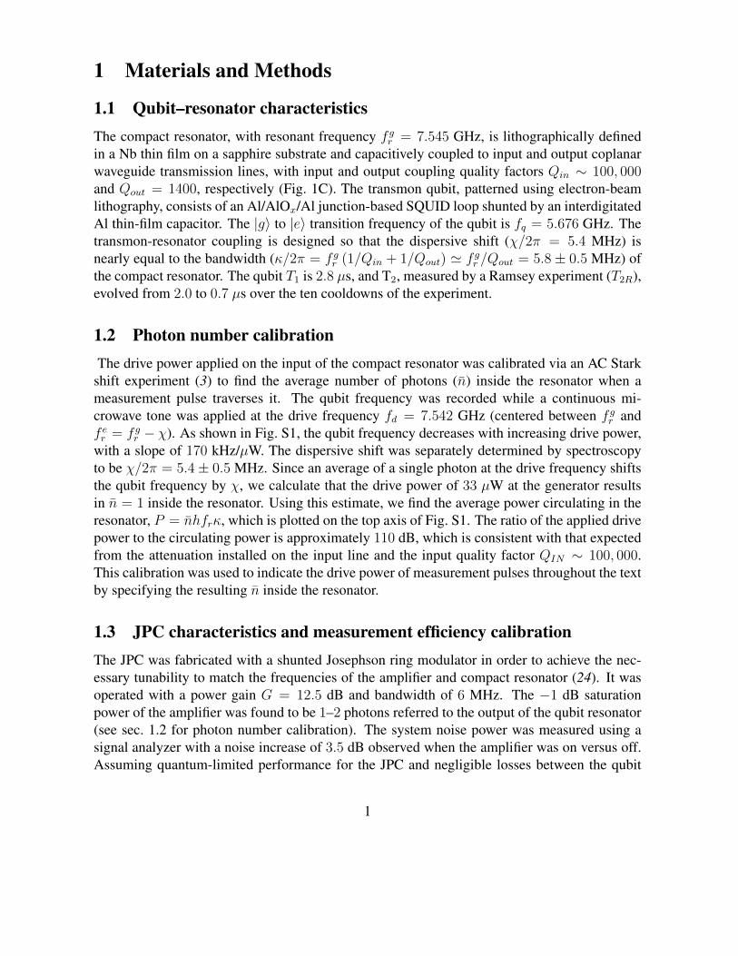
1.1 Qubit–resonator characteristicsThe compact resonator, with resonant frequency f gr = 7.545 GHz, is lithographically definedin a Nb thin film on a sapphire substrate and capacitively coupled to input and output coplanarwaveguide transmission lines, with input and output coupling quality factors Qin ∼ 100, 000and Qout = 1400, respectively (Fig. 1C). The transmon qubit, patterned using electron-beamlithography, consists of an Al/AlOx/Al junction-based SQUID loop shunted by an interdigitatedAl thin-film capacitor. The |g〉 to |e〉 transition frequency of the qubit is fq = 5.676 GHz. Thetransmon-resonator coupling is designed so that the dispersive shift (χ/2π = 5.4 MHz) isnearly equal to the bandwidth (κ/2π = f gr (1/Qin + 1/Qout) ' f gr /Qout = 5.8± 0.5 MHz) ofthe compact resonator. The qubit T1 is 2.8 µs, and T2, measured by a Ramsey experiment (T2R),evolved from 2.0 to 0.7 µs over the ten cooldowns of the experiment.

1.2 Photon number calibrationThe drive power applied on the input of the compact resonator was calibrated via an AC Stark

shift experiment (3) to find the average number of photons (n) inside the resonator when ameasurement pulse traverses it. The qubit frequency was recorded while a continuous mi-crowave tone was applied at the drive frequency fd = 7.542 GHz (centered between f gr andf er = f gr − χ). As shown in Fig. S1, the qubit frequency decreases with increasing drive power,with a slope of 170 kHz/µW. The dispersive shift was separately determined by spectroscopyto be χ/2π = 5.4± 0.5 MHz. Since an average of a single photon at the drive frequency shiftsthe qubit frequency by χ, we calculate that the drive power of 33 µW at the generator resultsin n = 1 inside the resonator. Using this estimate, we find the average power circulating in theresonator, P = nhfrκ, which is plotted on the top axis of Fig. S1. The ratio of the applied drivepower to the circulating power is approximately 110 dB, which is consistent with that expectedfrom the attenuation installed on the input line and the input quality factor QIN ∼ 100, 000.This calibration was used to indicate the drive power of measurement pulses throughout the textby specifying the resulting n inside the resonator.

1.3 JPC characteristics and measurement efficiency calibrationThe JPC was fabricated with a shunted Josephson ring modulator in order to achieve the nec-essary tunability to match the frequencies of the amplifier and compact resonator (24). It wasoperated with a power gain G = 12.5 dB and bandwidth of 6 MHz. The −1 dB saturationpower of the amplifier was found to be 1–2 photons referred to the output of the qubit resonator(see sec. 1.2 for photon number calibration). The system noise power was measured using asignal analyzer with a noise increase of 3.5 dB observed when the amplifier was on versus off.Assuming quantum-limited performance for the JPC and negligible losses between the qubit

1

resonator and amplifier, this places a bound on the quantum efficiency of the measurementchain of η ≤ 0.55± 0.03.

The calibration of n in sec. 1.2 provides an alternate estimate for the measurement efficiencyη, since it is related to the apparent measurement strength Im/σ. The apparent measurementstrength is given by

Im/σ =√

2nηNm sin(ϑ/2), (1)

where ϑ = 75± 1 for our experiment (Fig. 1B) and Nm is the number of elementary measure-ments performed. The value of ϑ is determined directly from measurement histograms moreaccurately than either χ or κ. Since we record the average of I(t) and Q(t) over a measurementtime Tm, we can write Nm ∼ BTm where B is the bandwidth of the measurement system. Theresonator bandwidth κ is an upper bound on B, though B may be reduced by the bandwidth ofthe JPC and the rest of the measurement chain. For Tm = 240 ns, we estimateNm to range from4 to 9. Using the data in Fig. 3 we find the apparent measurement strength Im/σ = 2.4 at n = 5,and therefore estimate η to range from 0.2 to 0.4. This estimate is in reasonable agreement withη ≤ 0.55 calculated from the noise rise experiment presented above.

1.4 Calculating ∂〈Z〉cσ∂Im

and ∂〈X〉cσ∂Qm

versus Im/σ

In order to produce the back-action data in Fig. 4A, the slopes of 〈Z〉c and 〈X〉c were extractedby fitting to data along the Qm = 0 and Im = 0 bins, respectively (see Fig. S2 for examplecurves and respective fits). In accordance with the form of zf given in Eq. (12), the data werefit to a hyperbolic tangent function. The data were weighted by the number of counts recordedin each bin to take into account the uncertainty due to variable counts per bin. The slope atIm = 0 was calculated from the fit coefficients. This routine is robust, and fails only whenzf changes rapidly compared to the bin spacing. For xf given in Eq. (12), the full form is ingeneral more complicated to fit, as its sinusoidal dependence on Qm is also suppressed by afactor exp (−I2m/σ2(1− η)). Thus, at large values of Im/σ, where the sinusoidal dependenceof xf on Qm would become relevant, xf also goes unconditionally to zero. This fit is furthercomplicated by T2 effects which additionally suppress xf . Consequently, xf was fit with a lineardependence, with the fit slope becoming less reliable at higher Im/σ.

The effective measurement strength Im/σ was separately extracted from measurement his-tograms. The entire experimental protocol shown in Fig. 3 was replicated with the first qubit ro-tation ofRx(0) andRx(π), which together with preparation of the ground state by post-selectionprepare |g〉 and |e〉, respectively. The most probable (Im, Qm) outcome was extracted with apeak finding algorithm and identified as (Ig,em , Qm), for the ground and excited states. Valuesfor Ig,em were found to be symmetric about the Qm = 0 axis, and the Im/σ = (Iem − Igm)/(2σ)was plotted as the horizontal coordinate in Fig. 4.

2

1.5 Purity of the qubit state after an imperfect measurementThe purity of the qubit state after measurement can be expressed by the length of its Bloch vec-tor, which should remain unity after a perfect measurement if the state was previously known.As shown in Eq. (13), in the case of an imperfect measurement (η < 1), this length is in gen-eral less than 1. However, the purity depends on the measurement outcome; sufficiently large|Im| outcomes correspond to purity approaching unity, while the purity is reduced for Im ∼ 0.This region of reduced purity is a general feature arising from the added classical uncertaintyin an imperfect measurement. As the apparent measurement strength increases, the region oflow purity is reduced and these outcomes become less probable. This behavior is verified ex-perimentally using the length of the Bloch vector squared plotted in Fig. S3A. The graph alsoshows the effect of T1 as an overall decrease of purity for outcomes corresponding to Im 0.This asymmetry arises in our data because the relaxation rate (Γ↓) is a factor of ten higher thanthe excitation rate (Γ↑). Therefore, a qubit in the excited state after the middle measurementcan relax before the final measurement, whereas a qubit in the ground state remains essentiallystationary.

We address the effect of T1 and T2 to first order by modifying Eq. (13), resulting in

R2 =(x2f + y2f

)e−2τ/T2 +

((zf + 1) e−τ/T1 − 1

)2(2)

= sech2

(ImImσ2

)e−

2I2mσ2

1−ηη e−2τ/T2 +

[(tanh

(ImImσ2

)+ 1

)e−τ/T1 − 1

]2.

In Fig. S3B, we plot this modified theory for measurement strengths corresponding to the datain part A which show good qualitative agreement between theory and experiment.

2 Supplementary Text

2.1 Theoretical analysisWe begin the description of the measurement process by considering the propagating modeassociated with the measurement pulse. The measurement pulse is assumed to have a temporalextent Tm, such that the pulse bandwidth 1/Tm is small compared to the bandwidth of theresonator and the JPC. The field quadratures of this mode are defined as I = (a + a†)/2 andQ = (a − a†)/2i. The average photon occupancy for a general coherent state of the mode,|α〉 is 〈α| a†a |α〉 = |α|2, while with this definition, the variance of each field quadrature isσ20 = 〈α| (I − 〈I〉)2 |α〉 = 〈α| (Q− 〈Q〉)2 |α〉 = 1/4. We can rewrite the field quadratures as

I

σ0= a+ a† and

Q

σ0=a− a†

i. (3)

Later in our derivation, these expressions will clarify the increase in variance due to both phase-preserving amplification and measurement inefficiency. Note that we can write the commutationrelation between I and Q as [I , Q] = 2iσ2

0 .

3

A note on the organization of this supplement: before discussing the measurement processas a whole in sec. 2.1.2, we first describe the crucial properties of the JPC in sec. 2.1.1.

2.1.1 Input-output relations of the JPC

An ideal, quantum-limited, phase-preserving amplifier like the JPC can be described as a twoport device (called signal and idler ports in our case), whose scattering properties are determinedby a drive applied to a third (pump) port (21). The input-output scattering relations for anideal JPC processing single-tone microwave pulses of duration much longer than its inversebandwidth can be written as

aoutSig =

√Gain

Sig + i√G− 1a† in

Idl , (4)

aoutIdl =

√Gain

Idl + i√G− 1a† in

Sig ,

where ain,outSig and ain,out

Idl are the incoming and outgoing field mode operators for the signal (Sig)and idler (Idl) ports and G is the pump-dependent amplifier power gain.

As shown in Fig. 1B, after further amplification through a HEMT amplifier, the output ofthe signal port is sent to a mixer allowing us to record both output quadratures. Therefore, usingEqs. (3) and (4) to write the output of the of the JPC signal mode referred to its input, we findthat we ultimately measure the two physical observable,

Im =1√GIoutSig = I inSig +

√G− 1√G

QinIdl

Qm =1√GQoutSig = Qin

Sig +

√G− 1√G

I inIdl. (5)

In general, these two observables do not commute and therefore they cannot be measured si-multaneously with arbitrary precision. However, in the limit of high gain G 1, the twoobservables converge to Im = I in

Sig + QinIdl and Qm = Qin

Sig + I inIdl, which do commute, and form a

complete set of commuting observables onHSig⊗HIdl, the joint Hilbert space of the signal andidler modes (see sec. 2.1.3 for details of the derivation).

2.1.2 Back-action on the qubit state after a phase-preserving measurement of the res-onator

To derive the back-action on the qubit due to the measurement of a qubit-resonator entangledstate, we assume that the state cg |g〉 ⊗ |αg〉 + ce |e〉 ⊗ |αe〉 is input to the signal port of theJPC which we suppose here to be ideal (inefficiency of the following measurement chain isdealt with later). As shown in sec. 2.1.1, the amplifier’s input state is actually a combinationof both signal and idler inputs, resulting in a modified pointer state |αs, αi〉. When the idlerhas no input signal, only quantum fluctuations are present, and the full state of the system canbe written as cg |g〉 ⊗ |αg, 0〉 + ce |e〉 ⊗ |αe, 0〉, where 0 represents vacuum input to the idler.

4

As shown in Fig. 1A, the pointer states |αg〉 and |αe〉 can be described by their mean outcomesαg = −Im + iQm, αe = Im + iQm, where we have assumed that the drive frequency of themeasurement pulse is centered between f gr and f er = f gr − χ as in the experiment. The meanoutcomes Im and Qm are related to other experimental parameters by I2m + Q2

m = |α|2 = nκTmand Im/Qm = tan (ϑ/2) = χ/κ. We perform a measurement of the observables (Im, Qm)and record the outcome (Im, Qm), in the process projecting the joint state of the signal andidler modes on to a unique eigenstate |ψIm,Qm〉 ∈ HS ⊗ HI . The new combined state of thequbit, signal and idler modes after projection is cg 〈ψIm,Qm | αg, 0〉 |g〉+ce 〈ψIm,Qm |αe, 0〉 |e〉]⊗|ψIm,Qm〉. The back-action of the measurement on the qubit state can be summarized as follows.An initial state of the qubit, represented by initial density matrix ρi, is conditionally transformedafter measurement with outcome (Im, Qm) to

ρimsmt−→ ρf (Im, Qm) =

MIm,QmρiM†Im,Qm

Tr(MIm,QmρiM

†Im,Qm

) , (6)

with a probability distribution for the measurement outcome (Im, Qm) given by P (Im, Qm) =

Tr(MIm,QmρiM

†Im,Qm

)(2).

The Kraus operator, MIm,Qm , calculated in sec. 2.1.4, is found to be

MIm,Qm =1√πe− (Qm−Qm)2

4σ2m

e− (Im+Im)2

4σ2m e

iImQm2σ2m 0

0 e− (Im−Im)2

4σ2m e

− iImQm2σ2m

, (7)

where σ2m = 1/2.

Let us now assume that the initial state ρi is the state polarized along the Bloch sphere y-axisso that (xi, yi, zi) = (0, 1, 0). The probability distribution for the outcome (Im, Qm) is given by

P (Im, Qm) =1

8πσ2m

exp

(−(Qm − Qm)2

2σ2m

)[exp

(−(Im − Im)2

2σ2m

)+ exp

(−(Im + Im)2

2σ2m

)].

(8)Firstly, P is found to be an equal superposition of two normal distributions centered on (−Im, Qm)and (Im, Qm) as expected since the qubit was in an equal superposition of |g〉 and |e〉. Sec-ondly, the variance of the outcomes in each quadrature is given by σ2

m = 1/2. Since the vari-ance of each quadrature of the coherent state |α〉 input to the signal port is given by σ2

0 =〈α| (ISig − 〈ISig〉)2 |α〉 = 〈α| (QSig − 〈QSig〉)2 |α〉 = 1/4, we find that σ2

m = 2σ20 . Thus, as

expected, phase-preserving amplification adds an extra half photon of noise which can be phys-ically identified to originate from the quantum noise input to the idler mode.

Next, using Eq. (6), we calculate the final density matrix ρf and find that the measurement

5

back-action corresponds to a final qubit Bloch vector :

xf (Im, Qm) = sech(ImImσ2m

)sin

(QmImσ2m

),

yf (Im, Qm) = sech(ImImσ2m

)cos

(QmImσ2m

), (9)

zf (Im) = tanh

(ImImσ2m

).

We see from Eq. (9), that xf , yf , zf can each take a continuum of values between −1 and 1 asexpected for a general finite-strength measurement. Further, since x2f + y2f + z2f = 1, the qubitremains in a pure state after the measurement despite the extra half photon of quantum noiseadded by the idler mode. This additional quantum noise forces the qubit to diffuse in all direc-tions on the 2-D surface of the Bloch sphere. However, as Eq. (9) shows, recording only theunpredictable outcome (Im, Qm) of a perfect measurement provides sufficient information forfull knowledge of the new state of the qubit after measurement. This principle that the unpre-dictable outcome of a perfect measurement provides sufficient information for full knowledgeof the back-action is naturally also true for the case of noiseless phase-sensitive amplification,though the details of the measurement back-action differ (8).

The effect of imperfections in the measurement chain arising from losses after the firstamplification provided by the JPC is taken into account by adding extra classical noise over thefundamental quantum noise. Let σ2 be the observed variance after an imperfect measurement.We define a measurement efficiency η = σ2

m/σ2 which by definition is no greater than unity.

This efficiency is linked to the inverse of Caves’ added noise number A through the relation1/η = A + 1/2, with A ≥ 1/2 for quantum-limited, phase-preserving amplification (19). Thisextra added classical noise results in a modification to the back-action in the following manner

(x, y, z)ηf (Im, Qm) =

∫ ∫dIdQ P(I,Q | Im, Qm) (x, y, z)f (I,Q), (10)

where P(I,Q|Im, Qm) denotes the conditional probability that a perfect measurement wouldgive the outcome (I,Q) while our imperfect one has given (Im, Qm). P(I,Q|Im, Qm) is calcu-lated in the sec. 2.1.5 to be

P(I,Q|Im, Qm) =1

2πη(1− η)σ2e− (Q−ηQm−(1−η)Qm)2

2η(1−η)σ2 e− (Im−I)2

2(1−η)σ2

(e− (I−Im)2

2σ2m + e

− (I+Im)2

2σ2m

)(e−

(Im−Im)2

2σ2 + e−(Im+Im)2

2σ2

) .(11)

Applying equation (10), we have that the final qubit state conditioned on the measurement

6

outcome (Im, Qm), expressed as a final qubit Bloch vector ~Sf = (xf , yf , zf ), is

xηf (Im, Qm) = sech(ImImσ2

)sin

(QmImσ2

+QmImσ2

(1− ηη

))e−

I2mσ2 ( 1−η

η ),

yηf (Im, Qm) = sech(ImImσ2

)cos

(QmImσ2

+QmImσ2

(1− ηη

))e−

I2mσ2 ( 1−η

η ), (12)

zηf (Im) = tanh

(ImImσ2

).

The length of the final Bloch vector squared, given by

R2 = x2f + y2f + z2f = 1− sech2

(ImImσ2

)(1− exp

(−2I2mσ2

1− ηη

)), (13)

will be in general less than 1 and therefore the qubit almost always fails to end in a pure statefor η < 1. Here the purity of the state after measurement is directly linked to the measurementoutcome, with large amplitude Im outcomes purer than those near zero.

The parameter Im/σ can be identified as the apparent measurement strength since the mea-surement becomes more strongly projective as Im/σ increases. To see this, note that Im out-comes in the center of the distribution (|Im| ∼ 0) become less probable, since, as shown fromEq. (8), the two Gaussian distributions centered on −Im and Im move further apart. Addition-ally, most Im outcomes correspond to a final Bloch vector ~Sf that is projected onto the z-axis.When Im/σ → ∞, we recover the situation of infinite-strength measurement where the onlypossible final qubit states are the poles of the Bloch sphere. Note that this strength depends bothon the strength of the readout and on the amplifier efficiency.

For weak apparent measurement strength (Im/σ, Qm/σ 1), we can approximate Eq. (12)to first order in (Im/σ,Qm/σ) as

xηf (Im, Qm) '(Imσ

)Qm

σ,

yηf (Im, Qm) ' 1, (14)

zηf (Im, Qm) '(Imσ

)Imσ.

This form shows that the back-action on the x- and z- component of the qubit state after mea-surement directly correspond to the I- and Q-component of the measurement outcome, respec-tively. The amplitude of the measurement back-action is symmetric in x and z, and determinedby the apparent measurement strength Im/σ.

7

Finally, we find that the correlation of the back-action with the measurement outcome is

σ∂xηf∂Qm

∣∣∣(Im,Qm)=(0,0)

=Imσ

cos

(QmImσ2

(1− ηη

))e−

I2mσ2 ( 1−η

η ),

σ∂yηf∂Qm

∣∣∣(Im,Qm)=(0,0)

= − Imσ

sin

(QmImσ2

(1− ηη

))e−

I2mσ2 ( 1−η

η ), (15)

σ∂zηf∂Im

∣∣∣Im=0

=Imσ.

which to first order in Im/σ, Qm/σ reduces to

σ∂xηf∂Qm

∣∣∣(Im,Qm)=(0,0)

≈ Imσ,

σ∂yηf∂Qm

∣∣∣(Im,Qm)=(0,0)

≈ 0, (16)

σ∂zηf∂Im

∣∣∣Im=0

≈ Imσ.

2.1.3 Showing Im and Qm form a complete set of commuting observables

We now prove that the two observables Im = ISig + QIdl and Qm = QSig + IIdl form a completeset of commuting observables on HSig ⊗ HIdl, the joint Hilbert space of the signal and idlermodes of the JPC. This result implies that a simultaneous measurement of these two observablesprojects the joint state of the signal and idler modes to a unique common eigenstate of bothobservables. First, the two observables commute since trivially

[ISig + QIdl, QSig + IIdl] = [ISig, QSig]− [IIdl, QIdl] = 0.

Next, in order to prove completeness, let us assume that there exists another observable O onHS ⊗HI such that

[ISig + QIdl, O] = 0 and [QSig + IIdl, O] = 0. (17)

We will show that O is necessarily of the form F (ISig + QIdl, QSig + IIdl), which does notdepend on QSig − IIdl and QIdl − ISig. To begin, O can in general be written as a functionf(ISig, QSig, IIdl, QIdl) of all four quadratures. We have,

[ISig + QIdl, O] = [ISig, f(ISig, QSig, IIdl, QIdl)] + [QIdl, f(ISig, QSig, IIdl, QIdl)]

= i~∂

∂QSigf(ISig, QSig, IIdl, QIdl)− i~

∂

∂IIdlf(ISig, QSig, IIdl, QIdl)

= i~∂

∂(QSig − IIdl)f(ISig, QSig, IIdl, QIdl).

8

Together with Eq. (17), this implies

∂

∂(QSig − IIdl)f(ISig, QSig, IIdl, QIdl) = 0.

Similarly, one finds∂

∂(QIdl − ISig)f(ISig, QSig, IIdl, QIdl) = 0.

Therefore f does not depend on QSig − IIdl and QIdl − ISig. Therefore f is only function ofISig + QIdl and QSig + IIdl, i.e. O = F (ISig + QIdl, QSig + IIdl). Hence we have proven thatIm = ISig + QIdl and Qm = QSig + IIdl form a complete set of commuting observables. This isthe mathematical representation of the physical intuition that the output of a high gain amplifieris ‘classical’. The ‘added noise’ of the amplifier accounts for the fact that, for vacuum input,while the signal and idler input ports obey 〈0| Q2 |0〉 = 〈0| I2 |0〉 = 1/4, the signal output portobeys 〈0| Q2

m |0〉 = 〈0| I2m |0〉 = 1/2.

2.1.4 Calculation of Kraus operator MIm,Qm

The Kraus operator MIm,Qm (2) is defined as

MIm,Qm =

(〈ψIm,Qm | αg, 0〉 0

0 〈ψIm,Qm | αe, 0〉

)(18)

Let us now calculate ξα(Im, Qm) = 〈ψIm,Qm|α, 0〉 needed to find MIm,Qm . The followingidentity follows from the definition of a coherent state

〈ψIm,Qm | aSig − iaIdl |α, 0〉 = α 〈ψIm,Qm |α, 0〉 = αξα(Im, Qm). (19)

However, we also have

〈ψIm,Qm| aSig − iaIdl |α, 0〉 = 〈ψIm,Qm|ISig + QIdl

2σ0|α, 0〉+ i 〈ψIm,Qm |

QSig − IIdl

2σ0|α, 0〉 . (20)

As |ψIm,Qm〉 is an eigenstate of ISig + QIdl with eigenvalue Im, we have

〈ψIm,Qm| ISig + QIdl |α, 0〉 = Im 〈ψIm,Qm|α, 0〉 = Imξα(Im, Qm). (21)

Now note that by the canonical commutation relation [ISig, QSig] = [IIdl, QIdl] = 2iσ20 , we have

〈ψIm,Qm |[ISig + QIdl, QSig − IIdl

]|ψIm,Qm〉 = 4iσ2

0〈ψIm,Qm|ψIm,Qm〉 = 4iσ20δ(Im−Im)δ(Qm−Qm),

(22)

9

where we have used the fact that the normalized eigenstates |ψIm,Qm〉 and |ψIm,Qm〉 are orthog-onal except if Im = Im and Qm = Qm. Furthermore, using the fact that ψIm,Qm and ψIm,Qm areeigenstates of ISig + QIdl, we have that

〈ψIm,Qm|[ISig + QIdl, QSig − IIdl

]|ψIm,Qm〉 = (Im − Im)〈ψIm,Qm |QSig − IIdl|ψIm,Qm〉. (23)

By Eq. (22) and (23) we have

〈ψIm,Qm|QSig−IIdl|ψIm,Qm〉 = 4iσ20

δ(Im − Im)δ(Qm − Qm)

(Im − Im)= −4iσ2

0δ(Qm−Qm)∂

∂Imδ(Im−Im).

(24)Therefore, we have

〈ψIm,Qm|QSig − IIdl|α, 0〉 =

∫ ∞−∞

∫ ∞−∞

dQmdIm 〈ψIm,Qm |QSig − IIdl|ψIm,Qm〉〈ψIm,Qm|α, 0〉

= −4iσ20

∂ξα∂Im

∣∣∣Im,Qm

. (25)

Equations (19), (20), (21) and (25) lead to the following partial differential equation:

∂

∂Imξα(Im, Qm) =

(α− Im)

4σ20

ξα(Im, Qm). (26)

In the same way, by considering 〈ψIm,Qm| aIdl − iaSig |α, 0〉, we have

∂

∂Qm

ξα(Im, Qm) =(−iα−Qm)

4σ20

ξα(Im, Qm). (27)

The general solution to the system of equations (26) and (27) is given by

ξα(Im, Qm) = Nα exp

(−1

2

(Im − α)2

(2σ0)2

)exp

(−1

2

(Qm + iα)2

(2σ0)2

), (28)

whereNα is a constant independent of Im andQm. Using the fact that∫dImdQm|ξα(Im, Qm)|2 =

1, we can show thatNα = π−1/2e−|α|2/2(2σ0)2eiζα where ζα is a phase term. One can further show

that this phase is independent of α by noting that

〈0, 0|α, 0〉 =

∫ ∫dImdQm 〈0, 0|ψIm,Qm〉 〈ψIm,Qm|α, 0〉

=1

πe−|α|

2/2(2σ0)2ei(ζα−ζ0)∫dIme

− 12

((I−α)2+I2)(2σ0)2

∫dQme

− 12

((Q+iα)2+Q2)(2σ0)2

= e−|α|2/2(2σ0)2ei(ζα−ζ0). (29)

10

By definition of the coherent state |α〉, we also know that 〈0, 0|α, 0〉 = e−|α|2/2(2σ0)2 . Therefore

ζα = ζ0, which indicates that the phase ζα is an arbitrary constant independent of α. Thiscompletes the calculation of ξα(Im, Qm).

From the definition of ξα(Im, Qm) = 〈ψIm,Qm |α, 0〉, we can see that |ξα(Im, Qm)|2 givesthe probability density function for recording an outcome (Im, Qm) when a coherent state |α〉 isinput at the signal mode of the amplifier and the vacuum state is present on the idler. Using (28)we can show that this implies that (Im, Qm) are random variables drawn from a normal distri-bution with mean (Re(α), Im(α)) and variance of 2σ2

0 = 1/2. Thus this derivation shows thatphase-preserving amplification increases the variance of a coherent state by a factor of two, orin other words the quantum noise of the idler mode adds an extra half photon worth of noise tothe input signal as expected from Caves’ theorem. We therefore define σ2

m = 2σ20 to be the vari-

ance of a coherent state observed at the output of an ideal, quantum-limited phase-preservingamplifier and can now write the Kraus operator MIm,Qm as

MIm,Qm =eiζ0√π

e− |αg |24σ2m e− (Im−αg)2

4σ2m e

− (Qm+iαg)2

4σ2m 0

0 e− |αe|

2

4σ2m e− (Im−αe)2

4σ2m e

− (Qm+iαe)2

4σ2m

. (30)

We can be further simplify M in the context of the current experiment. We take αg ≡−Im + iQm and αe ≡ Im + iQm, and note that dividing the matrix M by a constant of unitmodulus would not change the dynamics of Eq. (6). Therefore,

M =1√πe− (Qm−Qm)2

4σ2m

e− (Im+Im)2

4σ2m e

iImQm2σ2m 0

0 e− (Im−Im)2

4σ2m e

− iImQm2σ2m

. (31)

2.1.5 Calculation of P(I,Q|Im, Qm)

The conditional probability P(I,Q|Im, Qm) that a perfect measurement would give outcome(I,Q) while an imperfect one has given (Im, Qm) can be calculated through Bayes rule.

P(I,Q|Im, Qm) =P(Im, Qm|I,Q)P (I,Q)∫ ∫dIdQP(Im, Qm|I,Q)P (I,Q)

where P (I,Q) is the probability of the measurement outcome (I,Q) given in equation (8).Since the extra added classical noise has a variance σ2 − σ2

m = (1− η)σ2, we have

P(Im, Qm|I,Q) =1

2π(1− η)σ2e− (Im−I)2

2(1−η)σ2 e− (Qm−Q)2

2(1−η)σ2 ,

which implies that∫ ∫dIdQP(Im, Qm|I,Q)P (I,Q) =

1

4πσ2e−

(Qm−Qm)2

2σ2

(e−

(Im−Im)2

2σ2 + e−(Im+Im)2

2σ2

).

11

Therefore P(I,Q|Im, Qm) is

P(I,Q|Im, Qm) =1

2πη(1− η)σ2e− (Q−ηQm−(1−η)Qm)2

2η(1−η)σ2 e− (Im−I)2

2(1−η)σ2

(e− (I−Im)2

2σ2m + e

− (I+Im)2

2σ2m

)(e−

(Im−Im)2

2σ2 + e−(Im+Im)2

2σ2

) .

12

5.67

5.66

5.65

Qub

it fr

eque

ncy

(GH

z)

200150100500

Drive power (µW)

1.00.50.0

Circulating power (fW)

slope = -170 kHz/µW

Fig. S1. Measurement strength calibration. Plot of qubit frequency as a function of applied drivepower used to calibrate the rate at which photons leave the resonator for a given drive power,and therefore the measurement strength. Using the slope of 170 kHz/µW and χ/2π = 5.4 MHz,we calculate that a drive power of 33 µW results in an average of 1 photon leaking out of theresonator in a bandwidth κ. The corresponding average circulating power P = nhfrκ is plottedon the top axis.

13

A B

<X>c

<Z>c

1

0.5

0

-0.5

-1

1

0.5

0

-0.5

-1

Qm / σIm / σ40-4 40-4

5x10-2

0.21.25

Drive (n)

Qm = 0 Im = 0

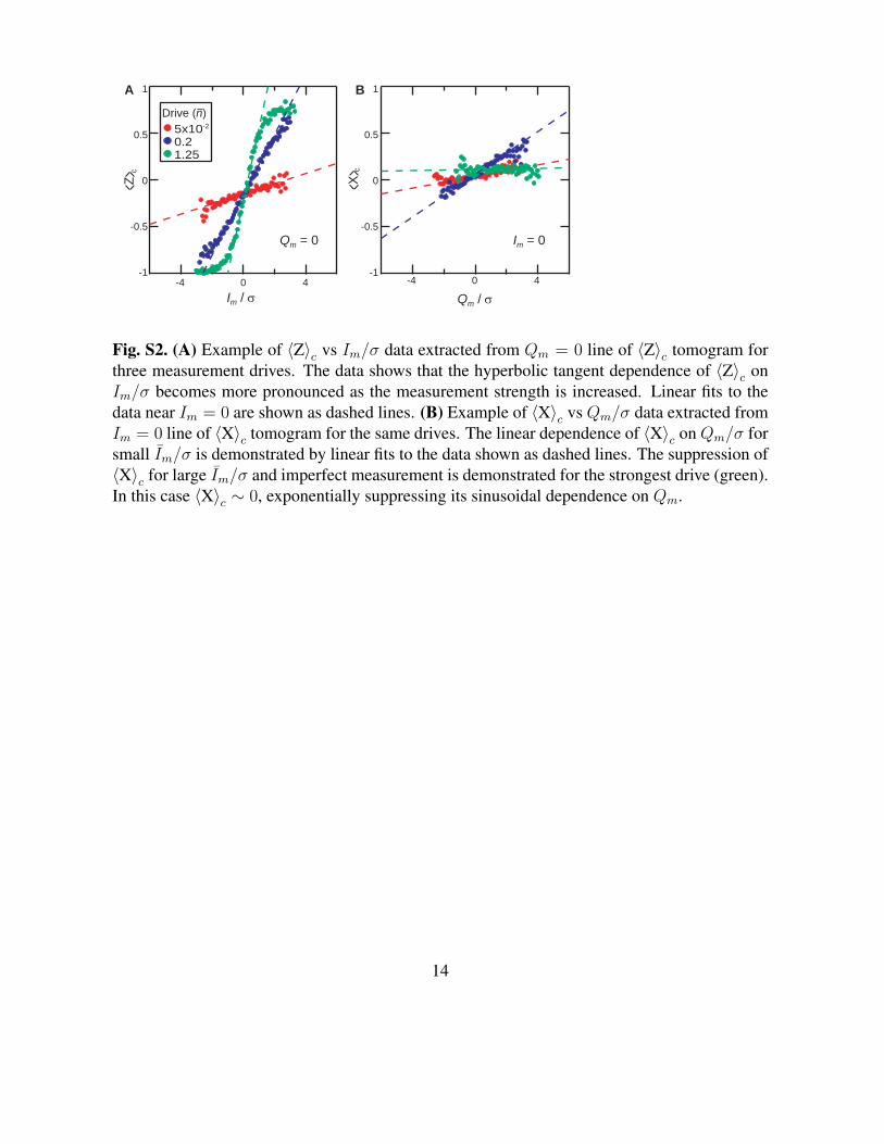
Fig. S2. (A) Example of 〈Z〉c vs Im/σ data extracted from Qm = 0 line of 〈Z〉c tomogram forthree measurement drives. The data shows that the hyperbolic tangent dependence of 〈Z〉c onIm/σ becomes more pronounced as the measurement strength is increased. Linear fits to thedata near Im = 0 are shown as dashed lines. (B) Example of 〈X〉c vs Qm/σ data extracted fromIm = 0 line of 〈X〉c tomogram for the same drives. The linear dependence of 〈X〉c on Qm/σ forsmall Im/σ is demonstrated by linear fits to the data shown as dashed lines. The suppression of〈X〉c for large Im/σ and imperfect measurement is demonstrated for the strongest drive (green).In this case 〈X〉c ∼ 0, exponentially suppressing its sinusoidal dependence on Qm.

14

1.0

0.8

0.6

0.4

0.2

-4 -2 0 2 4

5 x 10-1 5

Drive (n)

Im / σ

<X>c2

+ <Y>c2 + <Z

>c2

0.8

0.6

0.4

0.2

0.0

x f2 +y

f2 +zf2

A

B

Fig. S3. Experimental (A) and theory (B) curves for the length of Bloch vector squared(〈X〉2c + 〈Y〉2c + 〈Z〉2c

)as a function of Im/σ for two measurement drives. (A) Data extracted

from conditional maps by performing a weighted average over Qm for each component 〈X〉c,〈Y〉c, 〈Z〉c and summing the squares of the results. (B) Theory curves from Eq. (2) for corre-sponding measurement drives and experimentally determined values of Im/σ, T1 and T2. Thevalue for η was chosen to be 0.55, the maximum value estimated from the noise rise measure-ment described in the main text.

15