quarry operations and property values: revisiting old and ... · phoenix center policy paper no. 53...
TRANSCRIPT

PHOENIX CENTER POLICY PAPER SERIES
Phoenix Center Policy Paper Number 53:
Quarry Operations and Property Values: Revisiting Old and Investigating New Empirical Evidence
George S. Ford, PhD R. Alan Seals, PhD
(March 2018)
© Phoenix Center for Advanced Legal and Economic Public Policy Studies, George S. Ford and R. Alan Seals (2018).
Phoenix Center Policy Paper No. 53 Quarry Operations and Property Values: Revisiting Old and Investigating New Empirical Evidence George S. Ford, PhD† R. Alan Seals, PhD
(© Phoenix Center for Advanced Legal & Economic Public Policy Studies, George S. Ford and R. Alan Seals (2018).)
Abstract: A large literature exists on the impact of disamenities, such as landfills and airports, on home prices. Less frequently analyzed is the effect of rock quarries on property values, and what little evidence is available is dated and conflicting. This question of price effects is a policy relevant one, with one study in particular used frequently to support “not in my backyard” campaigns against new quarry sites. In this POLICY
PAPER, we revisit the literature and conduct a new analysis of the price effects of quarries, estimating the effect of quarries on home prices with data from four locations across the United States and a wide range of econometric specifications and robustness checks along with a variety of temporal circumstances from the lead-up to quarry installation to subsequent operational periods. We find no compelling statistical evidence that either the anticipation of, or the ongoing operation of, rock quarries negatively impact home prices. Our study likewise highlights a number of shortcomings in the empirical methodologies generally used to estimate the effect of disamenities on real estate prices. First and foremost, many existing studies are naïve as to the empirical conditions necessary to identify a causal relationship and do not establish credible strategies to estimate the counter-factual outcome. Second, the inclusion of “distance to the site” regressors in hedonic models is shown to be an unreliable statistical method. Using the method of randomized inference, the null hypothesis of “no effect” of placebo quarries is rejected in as much as 93% of simulations.
† Chief Economist, Phoenix Center for Advanced Legal & Economic Public Policy Studies. The views expressed in this paper are the authors’ alone and do not represent the views of the Phoenix Center or its staff.
Adjunct Fellow, Phoenix Center for Advanced Legal & Economic Public Policy Studies; Associate Professor of Economics and Director of Graduate Studies – Auburn University.

2 PHOENIX CENTER POLICY PAPER [Number 53
Phoenix Center for Advanced Legal and Economic Public Policy Studies www.phoenix-center.org
TABLE OF CONTENTS
I. Background .................................................................................................... 3 II. Empirical Framework ................................................................................... 6
A. Quantifying the Effect of a Quarry on Housing Prices ..................... 7 B. A Numerical Example ........................................................................... 8 C. Key Assumptions for Estimating Causal Effects ............................... 9
III. Revisiting the Hite Report ........................................................................... 12 A. A Review of Empirical Methods ........................................................ 14 B. National Lime & Stone Quarry in Delaware, Ohio ......................... 16
1. Alternative Estimation Approaches .............................................. 19 2. Coarsened Exact Matching ............................................................. 21
C. Rogers Group Quarry near Murfreesboro, Tennessee .................... 22 D. Randomized Inference and the Implausibility of the Model ......... 24 E. Spurious Regression and the Search for Results .............................. 26
IV. A Difference-in-Difference Approach ...................................................... 29 A. The Empirical Model ............................................................................ 30 B. Vulcan Quarry in Gurley, Alabama ................................................... 31 C. Austin Quarry in Madera County, California .................................. 33
V. Conclusions .................................................................................................. 38 Appendix 1. Map of National Lime & Stone Quarry near ......................... 40 Delaware, Ohio .................................................................................................. 40 Appendix 2. Map of Rogers Group Quarry near Murfreesboro,
Tennessee ..................................................................................................... 41 Appendix 3. Census Block Population Growth Near Rogers Group
Quarry near Murfreesboro, Tennessee .................................................... 42 Appendix 4. Illustrative Map of Random Locations Used for
Randomized Inference Analysis for Delaware County ......................... 43 Appendix 5. Vulcan Quarry near Gurley, Alabama .................................... 44 Appendix 6. Map of Austin Quarry Site in Madera County, California .. 45

Winter 2018] QUARRY OPERATIONS AND PROPERTY VALUES 3
Phoenix Center for Advanced Legal and Economic Public Policy Studies www.phoenix-center.org
I. Background
Odds are that underneath your feet is a construction material made of sand, crushed stone, and gravel. These construction materials are an essential ingredient into nearly every construction project, from residential housing, office buildings, retail outlets, entertainment structures, to the roads that connect them.1 Sand, rock and gravel are literally the foundation of economic development, but their extraction process can generate dust, noise, vibration, and truck traffic. While modern technologies and methods have greatly reduced quarries’ impact, the environmental and economic consequences of quarry operations receive considerable attention, often in the form of “not in my backyard” (or “NIMBY”) campaigns opposing quarry expansions or new sites. Choosing a quarry site is a delicate task. While a quarry may be best located far from residential density on NIMBY concerns, it also needs to be near the final point of demand due to its high transportation cost. Quarries must balance the need to be both “near” and “far,” so they are typically found on the outskirts of cities and towns.
A key NIMBY complaint in the siting and expansion of quarries is the effect of the operations on nearby home values. According to Census data, housing amounts to about 70% of the average American’s net wealth, so naturally homeowners are sensitive to any adverse effect, real or imagined, on property values.2 Despite NIMBY opposition, nearly all the evidence on quarry operations finds no price effect. Frequently mentioned studies include Rabianski and Carn (1987) and Dorrian and Cook (1996), both of which find no relationship between appreciation rates of property values near to and far from quarries.3 An
1 2014 Minerals Yearbook, Construction Sand and Gravel, U.S. Geological Survey (2014) at p. 1 (available at: https://minerals.usgs.gov/minerals/pubs/commodity/sand_&_gravel_construction/myb1-2014-sandc.pdf) (“Construction sand and gravel is a traditional basic building material and is one of the earliest materials used by humans for dwellings and later for outdoor areas such as paths, roadways, and other constructs. Despite the relatively low, but increasing, unit value of its basic products, the construction sand and gravel industry is a major contributor to and an indicator of the economic well-being of the Nation”).
2 Wealth, Asset Ownership, & Debt of Households Detailed Tables: 2013, U.S. Census Bureau (2017) (available at: https://www.census.gov/data/tables/2013/demo/wealth/wealth-asset-ownership.html).
3 A.M. Dorrian and C.G. Cook, Do Rock Quarry Operations Affect Appreciation Rates of Residential Real Estate, Working Paper (1996); J. Rabianski and N. Carn, Impact of Rock Quarry
(Footnote Continued. . . .)

4 PHOENIX CENTER POLICY PAPER [Number 53
Phoenix Center for Advanced Legal and Economic Public Policy Studies www.phoenix-center.org
even earlier study conducted for the U.S. Bureau of Mines in 1981 also found no consistent relationship between quarry operations and the prices of nearby homes.4 There are a number of consulting reports on the question, and none report price attenuation attributable to a quarry.5
Opposition to quarries based on home valuations relies universally on a report by Professor Patricia Hite (2006).6 This brief, 250-word study (hereinafter the “Hite Report”) analyzes data from a few thousand homes sales (apparently in the mid-to-late 1990s) around a single quarry in Delaware, Ohio. Using an unconventional regression model and data on transactions occurring decades after the quarry opened, the Hite Report finds a positive relationship between home prices and distance from the quarry. Based on that evidence, the Hite Report concludes that quarries reduce home values. Yet, the Hite Report’s methods and data do not support a causal interpretation.
As economic development marches on, new quarries will be required to satisfy the demand for basic building materials. In light of the mostly dated and conflicting evidence on the effect of quarries on housing prices, this POLICY PAPER offers new evidence, and a review of old evidence, on the relationship between housing prices and rock quarries. First, given its frequent use by NIMBY opposition to quarries, we revisit the Hite Report, analyzing home sales data
Operations on Value of Nearby Housing, Prepared for the Davidson Mineral Properties (August 25, 1987).
4 M. Radnor, D. Hofler, et al., Social, Economic and Legal Consequences of Blasting in Strip Mines and Quarries, U.S. Bureau of Mines (May 1981) (available at: http://www.cdc.gov/niosh/nioshtic-2/10006499.html).
5 See, e.g., Study of Impact of Proposed Quarry on The Real Estate Values of Surrounding Residential Property in Raymond, New Hampshire, Crafts Appraisal Associates Ltd. (April, 2009) (“The evidence does however suggest that the overall marketplace does not react to an influence such as a quarry with a measurable negative reaction as it relates to sale price.”); Martin Marietta New Design Quarry: Analysis of Effect on Real Estate Values, Stagg Resources Consultants, Inc. (November 17, 2008); A Property Valuation Report: Affect [sic] of Sand and Gravel Mines on Property Values, Banks and Gesso, LLC (October 2002); Impacts of Rock Quarries on Residential Property Values in Jefferson County, Colorado, Banks and Gesso, LLC (May 1998); R.J. McKown, Analysis of Proposed Sand & Gravel Quarry: Granite Falls, WA, Schueler, McKown & Keenan, Inc. (September 25, 1995).
6 D. Hite, Summary of Analysis: Impact of an Operational Gravel Pit on House Values: Delaware County, Ohio, Working Paper (2006). We assign the date “2006” as is conventional, but that year is merely the recording stamp date on the document when it was filed in some type of proceeding. We do not know whether a more detailed analysis was provided at some point. We have never seen such a document cited and were unable to locate it.

Winter 2018] QUARRY OPERATIONS AND PROPERTY VALUES 5
Phoenix Center for Advanced Legal and Economic Public Policy Studies www.phoenix-center.org
around the same Delaware-Ohio quarry. Despite replicating both the location and methods of the Hite Report, our regression analysis finds that prices fall—not rise—as distance from the quarry increases. This result conflicts with that appearing in the Hite Report, so we look for more evidence by analyzing data on homes sales near a quarry outside of Murfreesboro, Tennessee, over the same time interval. Again, we find prices fall as distance from the quarry increases.
We are reluctant, however, to claim this evidence implies quarries raise home prices. Rather, we conclude, based on the method of randomized inference and other tests, that the Hite Report’s method is unreliable. Using a simulation of pseudo-treatments, we find that the null hypothesis that home prices rise or fall in distance from a randomly selected location is rejected in no less than 67% of cases at the 10% nominal significance level. Estimating price-distance relationships, especially without explicitly considering selection bias, is a highly-unreliable statistical procedure. The nature of real estate markets do not permit the effect of quarries to be identified with such naïve empirical tests.
Second, using data on home sales near a relatively new quarry in Gurley, Alabama, we augment the Hite-style analysis with a difference-in-differences estimator, which quantifies the price-distance relationship both before-and-after operations begin. By exploiting the timing of the quarry buildout and the location of home sales with respect to the quarry, we can credibly identify a causal relationship, at least in theory. Unlike the analysis for Delaware and Murfreesboro, home prices rises in distance from the Gurley quarry site, but do so before the quarry becomes operational. After operations begin in 2013, the positive effect of distance is attenuated, again suggesting a positive effect of quarries on housing values.
One critique of our Gurley analysis is that market participants shift price forecasts downward in response to the prospect of a quarry so that the deleterious effects of the quarry could be realized before the quarry opens. Quarry site approvals normally take a decade or so, providing ample time for anticipatory responses to valuation fears. To address this concern, we analyze transactions near a recently approved quarry in Madera County, California. Using a difference-in-differences estimator in conjunction with Coarsened Exact Matching, we test for the anticipatory effect of the proposed quarry on nearby housing prices located along the major roadways serving the site. We find no evidence the quarry reduced housing prices. If anything, relative home prices rose near the quarry site.
While our evidence suggests that quarries do not reduce, but may increase, home prices, our analysis suggests more than anything that the identification of

6 PHOENIX CENTER POLICY PAPER [Number 53
Phoenix Center for Advanced Legal and Economic Public Policy Studies www.phoenix-center.org
the effect of quarries on prices is a very difficult problem, facing many conceptual and practical obstacles. We do not resolve all these difficulties. That said, we can conclude the evidence strongly implies the Hite Report and its methods are unreliable. Further analysis is, as usual, encouraged.
This paper is outlined as follows. First, we discuss the empirical requirements of quantifying a plausibly causal relationship between property values and quarry operations. Second, we revisit the Hite Report, estimating the price-distance relationship for the same quarry in Delaware, Ohio, and replicating the analysis for a quarry near Murfreesboro, Tennessee. Using a simulation method, we demonstrate the futility of estimating the price effects of quarries using the method proposed in the Hite Report. Third, we turn to the estimation of causal effects using the difference-in-differences estimator for quarry sites in Gurley, Alabama, and Madera County, California. Across multiple methods, we find, if anything, that home prices near quarries rise, not fall. In all, however, we believe our analysis best supports the hypothesis of “no effect” of quarries, or the announcement of quarries, on home prices. Conclusions are provided in the final section.
II. Empirical Framework
Disamenities such as landfills, airports, windfarms and prisons may plausibly reduce the prices of nearby homes. Such effects have been widely studied.7 Modern empirical methods for observational data based on the Rubin Causal Model, however, suggest that much of the work may offer biased estimates of such disamenities because much it looks only at prices after the “treatment,” making it difficult to address selection bias.8 To conclude that a disamenity reduces home values, the researcher’s interest must be in the causal effect of an amenity or disamenity on property values. Using only post-treatment prices is problematic since the locations of amenities and disamenities are not randomly selected, and
7 Other disamenities that may affect property values, airports and waste disposal, are frequently opposed by homeowners. See, e.g., J.P. Nelson, Airport and Property Values: A Survey of Recent Evidence, 14 JOURNAL OF TRANSPORT ECONOMICS AND POLICY 37-52 (1980) (available at: http://www.bath.ac.uk/e-journals/jtep/pdf/Volume_X1V_No_1_37-52.pdf); J.B. Braden, X. Feng, and D. Won, Waste Sites and Property Values: A Meta-Analysis, 50 ENVIRONMENTAL AND RESOURCE
ECONOMICS 175-201 (2011).
8 Excellent resources on the modern methods of causal inference for economic analysis include G.W. Imbens and J.M. Wooldridge, Recent Developments in the Econometrics of Program Evaluation, 47 JOURNAL OF ECONOMIC LITERATURE 5-86 (2009); J.D. Angrist and J. Pischke, MOSTLY
HARMLESS ECONOMETRICS: AN EMPIRICIST'S COMPANION (2008); and J.D. Angrist and J. Pischke, MASTERING ‘METRICS: THE PATH FROM CAUSE TO EFFECT (2015).

Winter 2018] QUARRY OPERATIONS AND PROPERTY VALUES 7
Phoenix Center for Advanced Legal and Economic Public Policy Studies www.phoenix-center.org
disamenities are typically located away from residential density to minimize impact and to placate NIMBY resistance.
The non-random selection of a quarry site greatly complicates the quantification of a quarry on housing prices due to selection bias. Finding that housing prices rise at increased distance from a quarry may merely reflect the economics of site choice (i.e., real estate is cheaper per unit in less densely populated areas on the outskirts of town) rather than any causal effect on property values. Also and consequently, empirical work may be frustrated by the lack of housing density near the site, rendering small sample sizes, which may, in turn, lead to the undue influence of outliers. Many quarries, especially new ones, have almost no housing within a mile or two of the site (the typical distance within which negative effects are claimed), as shown in the maps provided in the Appendices. And, given the lengthy approval process, if a quarry does affect housing prices, then such effects may occur prior to operations by an “announcement effect.” In conducting empirical work on quarries and housing prices, the researcher must address, and deal with the theoretical and empirical consequences of, the non-random nature of site location.
A. Quantifying the Effect of a Quarry on Housing Prices
Resistance to new quarry sites (or the expansions of old ones) based on property values rests exclusively on the Hite Report. In that report, the effect on prices is quantified by comparing the mean, quality-adjusted transactions prices around the quarry outside of Delaware, Ohio, as the home’s distance from the quarry increases. This “experiment,” however, has little hope of accurately measuring the effect of quarries on home prices.
To better grasp the nature of the problem, let there be two types of residential locations: (1) locations proximate to and potentially affected by quarry operations (labeled N, for “near”); and (2) locations distant from and entirely unaffected by quarry operations (labeled F, for “far”). Also, let there be two periods: the period prior to (t = 0) and after (t = 1) the initiation of quarry operations. For now, assume the approval process is instantaneous and that the quality and type of homes in the two locations are very similar (or, that such differences can be accounted for by statistical methods).
Prior to quarry operations homes sell for the average price NP0 if near the
future location of the quarry and FP0 otherwise. (A numerical example is provided
later.) For various reasons, these prices need not be equal. After quarry operations
begin, the average, quality-adjusted prices for houses are NP1 and FP1 . The

8 PHOENIX CENTER POLICY PAPER [Number 53
Phoenix Center for Advanced Legal and Economic Public Policy Studies www.phoenix-center.org
differences in the prices across time (P1 - P0) are N and F. Other things constant, the effect of the quarry operations can be measured as,
N F N N F FP P P P1 0 1 0 , (1)
where is the difference-in-differences (“DiD”) estimator.9 The DiD estimator looks for a difference in outcomes after the treatment that is difference than the differences in outcomes before the treatment (thus, explaining the term difference-in-differences). Under certain conditions, the DiD estimator plausibly measures the causal effect of the quarry.
Many studies of the effect of amenities or disamenities on housing values looks only at the difference between near and far locations in the post-treatment period,
or the difference in NP1 and FP1 (or 1). This post-treatment approach is the one
used in the Hite Report, where all the data is from sales decades after the quarry operations began. If, however, there is a difference in prices before the quarry operations begin, this post-operations difference is clearly not a measure of the effect of proximity to the quarry. A numerical example may prove helpful.
B. A Numerical Example
Before a quarry opens, assume the average, quality-adjusted price for a home near the quarry site is $80,000, but the average price is $100,000 for homes far from the future quarry site. Thus, there is a $20,000 or 20% difference in prices prior to quarry operations, perhaps reflecting the lack of locational rents for homes far from residential density. Plainly, since quarry operations have not begun, this difference cannot be attributed to the quarry. In fact, the quarry site may have been chosen because of the lower property values or lack of residential housing in the area.
As a benchmark case, say that the quarry operations once initiated have no effect on property values and the sales prices of homes are unchanged after quarry operations begin ($80,000 and $100,000, respectively). If a researcher were to
9 See, e.g., B.D. Meyer, Natural and Quasi-Experiments in Economics, 13 JOURNAL OF BUSINESS &
ECONOMIC STATISTICS 151-161 (1995); J.D. Angrist and A.B. Krueger, Empirical Strategies in Labor Economics, in HANDBOOK OF LABOR ECONOMICS Vol. 3A (eds., O. Ashenfelter and D. Card) (1999); S. Galiani, P. Gertler, and E. Schargrodsky, Water for Life: The Impact of the Privatization of Water Services on Child Mortality, 113 JOURNAL OF POLITICAL ECONOMY 83-123 (2005); D. Card, The Impact of the Mariel Boatlift on the Miami Labor Market, 13 INDUSTRIAL AND LABOR RELATIONS REVIEW 245-257 (1990).

Winter 2018] QUARRY OPERATIONS AND PROPERTY VALUES 9
Phoenix Center for Advanced Legal and Economic Public Policy Studies www.phoenix-center.org
simply compare prices based on distance from the quarry after operations begin, then a difference of 20% would be found. Yet, that difference existed prior to the quarry’s opening, and thus the quarry did not cause that difference, implying any causal claim made about that difference is mistaken. The truth (by assumption) is
that the quarry had no effect. The DiD estimator () is, in fact, zero, correctly identifying the causal effect of the quarry [= (80,000 – 80,000) – (100,000 – 100,000)].
Assume instead that the quarry does reduce prices for nearby homes. Let the post-quarry average prices be $70,000 near and $100,000 far from the quarry, other things constant.10 Prices near the quarry fall by $10,000 and those far from the quarry are unchanged. The DiD estimator accurately quantifies the effect of the quarry, which is a $10,000 reduction in value [= (70,000 – 80,000) – (100,000 – 100,000)]. Looking at data after the quarry operations begin, alternately, which is the Hite Report’s approach, would find an effect size of $30,000 [=70,000 – 100,000], or three times the true effect. Selection bias accounts for the $20,000 error in the estimated effect.
Ideally, then, to properly identify the causal effect of a quarry operation, the researcher must observe prices both before and after the quarry may reasonably be expected to affect housing prices (among other considerations such as the similarity in pricing trends prior to the treatment). The analysis of transactions occurring well after the quarry opens offers little hope for quantifying the effect of the quarry, absent unique circumstances. Certainly, the empirical demands are considerable, and the identification of the causal effect must be explicitly set forth and proper empirical methods applied.
C. Key Assumptions for Estimating Causal Effects
With regard to the location of homes and quarries, we do not have the luxury of experimental data. Rather, the data is observational and the data generation process occurs over many decades. The observational nature of the data is crucial: quarry site and housing locations are non-random and not independent of economic activity near the site or each other. Thus, research on the price effects of quarry sites must pay careful attention to selection bias, which is caused by the non-random process by which sites are chosen to avoid residential density but still
10 For instance, a large condominium complex may have built near the quarry. The researcher must adjust for the difference in average prices resulting from this changing mix of household types).
(Footnote Continued. . . .)

10 PHOENIX CENTER POLICY PAPER [Number 53
Phoenix Center for Advanced Legal and Economic Public Policy Studies www.phoenix-center.org
remain close to the point of demand for aggregates (i.e., sand, stone and gravel). Thus, the “treatment” and “outcome” are related through observed and potentially unobserved factors.11
As explained by Imbens and Wooldridge (2009), when estimating the causal treatment effect in observational studies the researcher must be alert to two key concepts stemming from selection bias: (1) unconfoundedness (or the conditional independence assumption) and (2) covariate overlap (or common support).12 Unconfoundedness implies that, conditional on observed covariates X, the treatment assignment probabilities are independent of potential outcomes. If we have a sufficiently rich set of observable covariates, then regression analysis including the variables X leads to valid estimates of causal effects. Since the X must be observed to be included in the regression model, this approach is often referred to as selection on observables. It is difficult to know and impossible to test whether the observed and included X are sufficient to guarantee unconfoundedness (so the regression error and treatment are uncorrelated), though some guidance is available through pseudo-treatment tests (as applied later).
The conditional independence assumption (or unconfoundedness) implies that the observed factors included in the statistical analysis fully account for all the differences in the types of homes sold both near and far from the quarry (or other site of interest).13 In quantifying the effect of education on income, for instance, it is not enough to simply compare the incomes of persons with and without a college education. Work ethic, for instance, affects both the probability that a person will obtain a college degree and his or her future income. A hard-working person may earn a higher income even without a college education. If work ethic cannot be observed, then a comparison of average incomes across those with and without a college degree does not measure the true value of a degree. The difference is a positively biased estimate of the payoff of education.
11 In regression analysis, this problem appears as a correlation between the regression residual and the treatment variable.
12 Supra n. 8.
13 That is, the regression model includes all the regressors needed to make the conditional near and far prices equal prior to the treatment.
(Footnote Continued. . . .)

Winter 2018] QUARRY OPERATIONS AND PROPERTY VALUES 11
Phoenix Center for Advanced Legal and Economic Public Policy Studies www.phoenix-center.org
The second factor to consider for the measurement of the causal effect is covariate overlap, which Imbens and Wooldridge (2009) observe is, after unconfoundedness, the “main problem facing the analyst.”14 This condition implies that the support of the conditional distribution of X for the control group overlaps completely with the conditional distribution of X for the treatment group. That is, the covariate distributions for the treated and untreated groups are sufficiently alike, thereby lending credibility to the extrapolations inherent to regression analysis between groups. If the characteristics of untreated observations (home far from the quarry) are very different from the treated observations (homes near to the quarry), then the projections from the controls to the treated units will be a poor one.
Say, for instance, that a sample used to assess the effect of an experimental cancer treatment includes only persons over 65 years old in the experimental treatment group (or simply treatment group) and only persons below 45 years old in the non- treatment group (or control group). The purpose of the control group is not simply a counterweight to the treatment group. Rather, the control group measures the outcomes for the treated group if that group did not receive the treatment. To fix ideas, what we actually want to estimate is what would the treatment group have looked like had they not been treated, which is the sole purpose of a control group. It is unreasonable to expect, we believe, that the survival outcomes of 45 year-old persons provides an approximation of survival outcomes of persons 65 years and over that did not receive the experimental treatment. To extrapolate this discussion to the case of housing values, if the control group includes almost all homes in a golf course community with swimming pools and the treatment group—the properties near some dis-amenity—includes mostly one-bedroom condominiums, then the difference in sale prices between the two is a nearly meaningless statistic. Regression models are powerful tools, but they cannot make up of for such large differences in characteristics across treatment and control groups (even if observable and included in the regression model as explanatory variables), which is important given that the control group is being “projected” onto the treatment group.
A number of statistical techniques are used to address confoundedness and covariate imbalance in observational studies. In a housing study, for instance, a researcher may choose the control group by finding a group of homes comparable to the treatment group—that is, similar square footage, amenities, lot sizes—from a population of homes unaffected by the treatment. This approach, which we
14 Imbens and Wooldridge, supra n. 8 at 43.

12 PHOENIX CENTER POLICY PAPER [Number 53
Phoenix Center for Advanced Legal and Economic Public Policy Studies www.phoenix-center.org
employ here, ensures that the characteristics of homes in the treatment and control groups are sufficiently similar, adding credibility to the control group as a suitable “stand in” for the treatment group if it had not received the treatment.
The Hite Report is silent on both of these key assumptions, and there is good reason to suspect the analysis fails on both counts. All the pricing data is for home sales occurring long after the quarry operation began and the regression model is quite basic, so the experiment is almost certainly plagued with selection bias. As for covariate overlap, from what few descriptive statistics are provided in the Hite Report we observe that the range of home prices within 0.5 miles of the quarry has a minimum of $80.1 and a maximum of $178.9 (in thousands). In contrast, the range of prices for homes further from the quarry is $60 to $798.6. This difference in the maximum prices is sizable, suggesting that the homes near the quarry may be very much unlike those far from the quarry, thus risking biased results of the effect of distance.
III. Revisiting the Hite Report
In NIMBY campaigns challenging quarry development, the Hite Report is the sole empirical analysis supporting the claim that quarries reduce housing prices. Subsequent works by Erickcek (2006), the Center for Spatial Economics (2009), Smith (2014), among others, conduct no new empirical analysis, choosing instead to extrapolate the Hite Report’s results to different locations (a questionable practice on its own).15
15 G.A. Erickcek, An Assessment of the Economic Impact of the Proposed Stoneco Gravel Mine Operation on Richland Township, W.E. Upjohn Institute for Employment Research (August 15, 2006) (available at: http://www.stopthequarry.ca/documents/US%20Study%20on%20the%20impact%20of%20pits%20quarries%20on%20home%20prices.pdf); The Potential Financial Impacts of the Proposed Rockfort Quarry, Center for Spatial Economics (February 26, 2009) (available at: http://wcwrpc.org/FinancialImpacts_RockfortQuarryCanada.pdf); G. Smith, Economic Costs and Benefits of the Proposed Austin Quarry in Madera County, Report (October 23, 2014) (available at: http://www.noaustinquarry.org/wp-content/uploads/2016/08/Austin-Quarry-Economics-Report.pdf). Other works relying on the Hite Report (directly or indirectly) include, e.g., M. Conklin, et al., The Quarry Proposed by St. Marys Cement Inc. for a Location Near Carlisle, Ontario Should Not be Permitted: Proponents’ Brief, 5 STUDIES BY UNDERGRADUATE RESEARCHERS AT GUELPH (2011) (available at: https://journal.lib.uoguelph.ca/index.php/surg/article/view/1338/2345); Business Suirvey and Economic Assessment of Locating a Quarry and Asphalt and Cement Plants within Aeortech Park, Group ATN Consulting, Inc. (October 13, 2014) (available at: http://stopthefallriverquarry.com/wp-content/uploads/2015/10/GATN_Aerotech_Park_FINAL_Report_Oct_13_2015-2.pdf); M.A. Sale,
(Footnote Continued. . . .)

Winter 2018] QUARRY OPERATIONS AND PROPERTY VALUES 13
Phoenix Center for Advanced Legal and Economic Public Policy Studies www.phoenix-center.org
This uniform reliance on the Hite Report is somewhat surprising. On the face of it, the report is a seven-page document consisting of 1.5 pages of double spaced text (about 250 words) along with a few tables and figures. It is more an “abstract” than it is a “study.” Moreover, even a brief review of the Hite Report points to a number of serious problems that should give any researcher pause. First, there are almost no details regarding model specification and few details on the data used. Not even descriptive statistics are provided. Second, the choice of model specification is entirely ad hoc, treating nearly identical variables (distance) differently with respect to functional form and using a non-standard and unnecessary estimation procedure. Such inconsistent, unconventional and inconvenient choices are symptomatic of ends-driven analysis. Third, no explanation is provided as to how the chosen model and analysis of transactions occurring decades after the quarry operations began might identify the effect of that particular quarry (or any new quarry) on housing prices. Selection bias is clearly a concern, but it is neither mentioned nor addressed. Fourth, no analysis is provided to suggest that the homes near the quarry are sufficiently similar to those distant from the quarry to provide reliable estimates of the effect of distance (i.e., covariate overlap). Comparing prices of the homes in rural areas on the outskirts of town to those near the local university risks confusing the vagaries of real estate development with the impact of the quarry.
Setting aside the question of causality for the moment, whether the relationship estimated in the Hite Report can be replicated is an important first step in evaluating the report’s credibility and the suitability of the methods used to answer this policy-relevant empirical question. To that end, we collect data on home sales within five-miles of the same quarry in Delaware, Ohio, evaluated in the Hite Report.16 It appears the data from the Hite Report was from the 1990’s (though it is impossible to be certain given the lack of detail), so we collect data on
Quarry Bad for Area, THE NEWS & ADVANCE (September 28, 2008) (available at: http://www.newsadvance.com/opinion/editorials/letters-to-the-editor-for-sunday-september/article_ca388ca4-14c7-534b-9b17-1b78d1cecc40.html).
16 Data is obtained from www.agentpro247.com. For all our analysis, we limit the prices to greater than $25,000 and less than $1,000,000, and look only at the “full” sales of single-family homes not in distress. The National Lime & Stone Quarry near Delaware, Ohio, is located near Latitude 40.281005 and Longitude -83.135828.
(Footnote Continued. . . .)

14 PHOENIX CENTER POLICY PAPER [Number 53
Phoenix Center for Advanced Legal and Economic Public Policy Studies www.phoenix-center.org
sales over the ten-year period 1998 through 2007.17 These data appear to immediately follow that used in the Hite Report but precedes the housing market crash in 2008 and the broader economic malaise that followed.18 For further analysis, we also collect data on sales near a quarry outside of Murfreesboro, Tennessee, over the same ten-year period.
A. A Review of Empirical Methods
To reproduce the Hite Report’s analysis, we obtain transactions prices on 2,114 single-family homes between 1998 through 2007 that are located within five miles of the National Lime & Stone Quarry near Delaware, Ohio. Using latitude and longitude coordinates, distance from each home to the center the quarry (D) is calculated. Other explanatory variables used the Hite Report include, for each transaction, the sale date (DATE), the distance to Delaware City (DDC), the house-to-lot size (H2L), the number of bathrooms (BATH), and the number of total rooms (TOTR). We measure the sale date as the year of sale; the Hite Report does not indicate how the sale date is measured.19
The regression model of the Hite Report takes the following general form,
k
it i j j i i tj
p D X1 0 , ,1
exp( ln )
, (2)
where pit is the transaction price (in thousands) for home i at time t, lnD is the natural log of distance from the quarry (in miles), and Xj are the k regressors listed
above (with coefficients j as coefficients).20 For reasons unexplained in the Hite Report, only the distance from the quarry is transformed by the natural log
17 See also D. Hite, The Impact of the Ajax Mine on Property Values, ARMCHAIRMAYOR.CA (March 5, 2015) (available at: https://armchairmayor.ca/2015/03/05/letter-the-impact-of-the-ajax-mine-on-property-values) (stating that the analysis was completed in 1996-1998).
18 Our data source does not offer data in the early-to-mid 1990s, so we cannot replicate the same time period as the Hite Report. We are trying to obtain such data for further analysis.
19 It is preferred to measure DATE as a fixed effects, as this specification requires prices to rise monotonically over time.
20 The variables in the model are listed at Hite Report, supra n. 6 at p. 3. A similar specification is used in D. Hite, A Hedonic Model of Environmental Justice, Working Paper (February 14, 2006) (available at: https://papers.ssrn.com/sol3/papers.cfm?abstract_id=884233).
Winter 2018] QUARRY OPERATIONS AND PROPERTY VALUES 15
Phoenix Center for Advanced Legal and Economic Public Policy Studies www.phoenix-center.org
transformation; distance from the city center (DCC) and the other regressors are not transformed. The specification seems purely ad hoc.
Equation (2) is non-linear in the parameters and must be estimated by Non-Linear Least Squares (“NLS”). This specification is highly irregular in econometric practice. Normally, hedonic models of housing prices are estimated by Ordinary Least Squares (“OLS”). A regression model quite similar to Equation (2) and very common in hedonic analysis is,
k
i t i j j i i tj
p D X, 1 0 , ,2
ln ln
, (3)
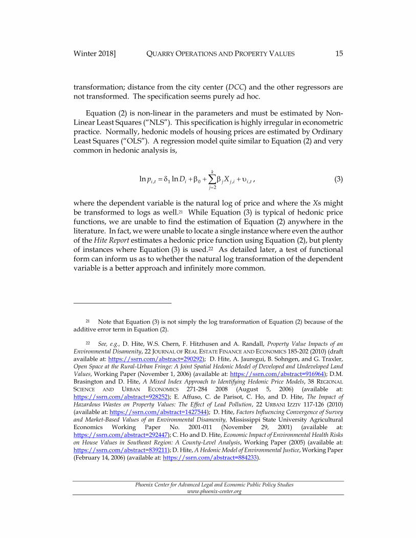
where the dependent variable is the natural log of price and where the Xs might be transformed to logs as well.21 While Equation (3) is typical of hedonic price functions, we are unable to find the estimation of Equation (2) anywhere in the literature. In fact, we were unable to locate a single instance where even the author of the Hite Report estimates a hedonic price function using Equation (2), but plenty of instances where Equation (3) is used.22 As detailed later, a test of functional form can inform us as to whether the natural log transformation of the dependent variable is a better approach and infinitely more common.
21 Note that Equation (3) is not simply the log transformation of Equation (2) because of the additive error term in Equation (2).
22 See, e.g., D. Hite, W.S. Chern, F. Hitzhusen and A. Randall, Property Value Impacts of an Environmental Disamenity, 22 JOURNAL OF REAL ESTATE FINANCE AND ECONOMICS 185-202 (2010) (draft available at: https://ssrn.com/abstract=290292); D. Hite, A. Jauregui, B. Sohngen, and G. Traxler, Open Space at the Rural-Urban Fringe: A Joint Spatial Hedonic Model of Developed and Undeveloped Land Values, Working Paper (November 1, 2006) (available at: https://ssrn.com/abstract=916964); D.M. Brasington and D. Hite, A Mixed Index Approach to Identifying Hedonic Price Models, 38 REGIONAL
SCIENCE AND URBAN ECONOMICS 271-284 2008 (August 5, 2006) (available at: https://ssrn.com/abstract=928252); E. Affuso, C. de Parisot, C. Ho, and D. Hite, The Impact of Hazardous Wastes on Property Values: The Effect of Lead Pollution, 22 URBANI IZZIV 117-126 (2010) (available at: https://ssrn.com/abstract=1427544); D. Hite, Factors Influencing Convergence of Survey and Market-Based Values of an Environmental Disamenity, Mississippi State University Agricultural Economics Working Paper No. 2001-011 (November 29, 2001) (available at: https://ssrn.com/abstract=292447); C. Ho and D. Hite, Economic Impact of Environmental Health Risks on House Values in Southeast Region: A County-Level Analysis, Working Paper (2005) (available at: https://ssrn.com/abstract=839211); D. Hite, A Hedonic Model of Environmental Justice, Working Paper (February 14, 2006) (available at: https://ssrn.com/abstract=884233).
16 PHOENIX CENTER POLICY PAPER [Number 53
Phoenix Center for Advanced Legal and Economic Public Policy Studies www.phoenix-center.org
The coefficient of primary interest in the Hite Report is 1, which measures the percent change in the transaction price for a percentage change in distance from the quarry (D), but only after the quarry operations began (see Eq. 1). In this specification (and also for Eq. 3), this elasticity is constant across the full range of
distance. With data on 2,812 sales, the Hite Report estimates the coefficient 1 to be 0.125, where the positive sign indicates the average sale price of homes is higher the further away the homes are from the quarry (statistically significant at the 1% level). The Hite Report concludes, as do subsequent reports that adopt the result, that this positive coefficient implies quarries reduce the price of nearby homes. As
detailed above, the positive sign on the coefficient 1 cannot reasonably be interpreted in this manner since the data is for sales occurring long after quarry operations began, among other concerns.
B. National Lime & Stone Quarry in Delaware, Ohio
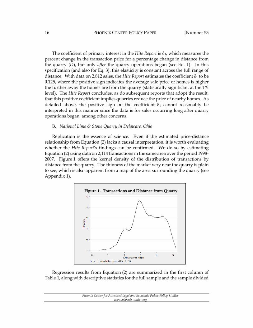
Replication is the essence of science. Even if the estimated price-distance relationship from Equation (2) lacks a causal interpretation, it is worth evaluating whether the Hite Report’s findings can be confirmed. We do so by estimating Equation (2) using data on 2,114 transactions in the same area over the period 1998-2007. Figure 1 offers the kernel density of the distribution of transactions by distance from the quarry. The thinness of the market very near the quarry is plain to see, which is also apparent from a map of the area surrounding the quarry (see Appendix 1).
Regression results from Equation (2) are summarized in the first column of Table 1, along with descriptive statistics for the full sample and the sample divided
Figure 1. Transactions and Distance from Quarry

Winter 2018] QUARRY OPERATIONS AND PROPERTY VALUES 17
Phoenix Center for Advanced Legal and Economic Public Policy Studies www.phoenix-center.org
into homes closer to the quarry than two miles and those further than that distance. The model has a Pseudo-R2 of 0.25, which is very close to that reported in the Hite Report (0.254).23 Five of the seven estimated coefficients (including the constant term) are statistically different from zero at the 1% level or better.
Table 1. Regression Results and Descriptive Statistics National Quarry near Delaware, Ohio
Coef (t-stat)
Mean (St. Dev)
N = 0 Mean
(St. Dev)
N = 1 Mean
(St. Dev)
lnD (1) -0.1413*** (-4.00)
1.166 (0.304)
1.227 (0.230)
0.518 (0.224)
DATE 0.0450*** (11.13)
2002.7 (2.952)
2002.5 (2.969)
2004.4 (2.125)
DDC 0.0409*** (5.92)
2.876 (2.139)
2.859 (2.207)
3.050 (1.207)
H2L -0.102 (-0.81)
0.1498 (0.1110)
0.148 (0.111)
0.1668 (0.102)
BATH 0.0419 (1.09)
1.806 (0.584)
1.788 (0.597)
1.995 (0.384)
TOTR 0.1398*** (7.59)
5.099 (1.016)
5.065 (1.031)
5.099 (1.016)
Constant -85.71*** (-10.57)
… … …
Pseudo-R2 0.250
Obs. 2,114 2,114 1,930 184
Statistical Significance: *** 1%, ** 5%, * 10%
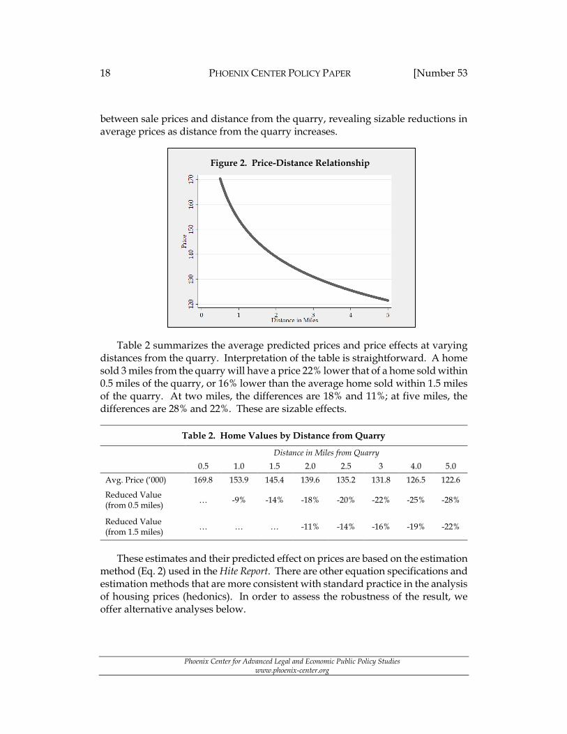
Despite using exactly the same regression model and data on sales around the same quarry, we find that the transaction prices of homes decrease (not increase) as the distance from the quarry increases. The negative coefficient (-0.141) is similar in size but different in sign from that found in the Hite Report (0.125) and is statistically significant at the 1% level. The estimated coefficient implies a 1% increase in distance reduces home average, quality-adjusted home prices by about 0.14%. Since the coefficient is less than unity, the price-distance relationship is subject to diminishing marginal returns.24 Figure 2 illustrates the relationship
23 The Pseudo-R2 is the squared correlation coefficient between the predicted value of the regression and the dependent variable.
24 For any fixed change in mileage, the percentage change falls as distance increases.
18 PHOENIX CENTER POLICY PAPER [Number 53
Phoenix Center for Advanced Legal and Economic Public Policy Studies www.phoenix-center.org
between sale prices and distance from the quarry, revealing sizable reductions in average prices as distance from the quarry increases.
Table 2 summarizes the average predicted prices and price effects at varying distances from the quarry. Interpretation of the table is straightforward. A home sold 3 miles from the quarry will have a price 22% lower that of a home sold within 0.5 miles of the quarry, or 16% lower than the average home sold within 1.5 miles of the quarry. At two miles, the differences are 18% and 11%; at five miles, the differences are 28% and 22%. These are sizable effects.
Table 2. Home Values by Distance from Quarry
Distance in Miles from Quarry
0.5 1.0 1.5 2.0 2.5 3 4.0 5.0
Avg. Price (‘000) 169.8 153.9 145.4 139.6 135.2 131.8 126.5 122.6
Reduced Value (from 0.5 miles)
… -9% -14% -18% -20% -22% -25% -28%
Reduced Value (from 1.5 miles)
… … … -11% -14% -16% -19% -22%
These estimates and their predicted effect on prices are based on the estimation method (Eq. 2) used in the Hite Report. There are other equation specifications and estimation methods that are more consistent with standard practice in the analysis of housing prices (hedonics). In order to assess the robustness of the result, we offer alternative analyses below.
Figure 2. Price-Distance Relationship

Winter 2018] QUARRY OPERATIONS AND PROPERTY VALUES 19
Phoenix Center for Advanced Legal and Economic Public Policy Studies www.phoenix-center.org
1. Alternative Estimation Approaches
As discussed above, Equation (2) is a non-standard method to estimate the relationship of interest. Normally, a researcher would avoid the non-linear Equation (2) and use the natural log of price to estimate Equation (3) by OLS. Statistical testing (such as the Box-Cox test of functional form) may be used to evaluate whether the linear or log-form of the dependent variable is preferred.25 Other advantages of Equation (3) over Equation (2) is that the linear equation is amenable to estimation by Median Regression (“MReg”) and Robust Regression (“RReg”), both of which are less sensitive to outliers in the data than is NLS or OLS.26 Outliers are common in home sales data, so it is sensible to evaluate the effect on the estimates by these alternative estimation procedures, especially when the results are used in a policy relevant setting that may have significant financial implications.27 We summarize the results from both methods.
Modern research on housing prices increasingly accounts for the spatial nature of real estate markets using new spatial methods.28 We estimate the price-distance
25 W.E. Griffiths, R.C. Hill and G.G. Judge, LEARNING AND PRACTICING ECONOMETRICS (1993) at pp. 345-7.
26 See, e.g., R. Koenker, QUANTILE REGRESSION (2005); B.S. Cade and B.R. Noon, A Gentle Introduction to Quantile Regression, 1 FRONTIERS IN ECOLOGY AND THE ENVIRONMENT 412-420 (2004) (available at: http://www.econ.uiuc.edu/~roger/research/rq/QReco.pdf); O.O. John, Robustness of Quantile Regression to Outliers, 3 AMERICAN JOURNAL OF APPLIED MATHEMATICS AND STATISTICS 86-88 (2015); P.J. Rousseeux and A.M. Leroy, ROBUST REGRESSION AND OUTLIER DETECTION (2005); R. Andersen, MODERN METHODS FOR ROBUST REGRESSION (2008); T.P. Ryan, MODERN REGRESSION
METHODS (2008).
27 C. Janssen, B. Söderberg and J. Zhou, Robust Estimation of Hedonic Models of Price and Income for Investment Property, 19 JOURNAL OF PROPERTY INVESTMENT & FINANCE 342-360 (2001); S.C. Bourassa, E. Cantoni and M. Hoesli, Robust Hedonic Price Indexes, 9 INTERNATIONAL JOURNAL OF HOUSING
MARKETS AND ANALYSIS 47-65 (2016).
28 Including papers by the Hite Report’s author. See, e.g., D.M. Brasington and D. Hite, Demand for Environmental Quality: A Spatial Hedonic Analysis, 35 REGIONAL SCIENCE AND URBAN ECONOMICS 57-82 (2005) (draft available at: https://ssrn.com/abstract=491244); see also J.M. Mueller and J.B. Loomis, Spatial Dependence in Hedonic Property Models: Do Different Corrections for Spatial Dependence Result in Economically Significant Differences in Estimated Prices?, 33 JOURNAL OF AGRICULTURAL AND
RESOURCE ECONOMICS 212-231 (2008) (available at: http://ageconsearch.umn.edu/bitstream/42459/2/MuellerLoomis.pdf); L. Osland, An Application of Spatial Econometrics in Relation to Hedonic House Price Modeling, 32 JOURNAL OF REAL ESTATE
(Footnote Continued. . . .)
20 PHOENIX CENTER POLICY PAPER [Number 53
Phoenix Center for Advanced Legal and Economic Public Policy Studies www.phoenix-center.org
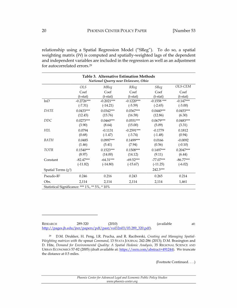
relationship using a Spatial Regression Model (“SReg”). To do so, a spatial weighting matrix (W) is computed and spatially-weighted lags of the dependent and independent variables are included in the regression as well as an adjustment for autocorrelated errors.29
Table 3. Alternative Estimation Methods National Quarry near Delaware, Ohio
OLS MReg RReg SReg OLS-CEM
Coef
(t-stat) Coef
(t-stat) Coef
(t-stat) Coef
(t-stat) Coef
(t-stat)
lnD -0.2726*** (-7.31)
-0.2021*** (-14.21)
-0.1220*** (-5.59)
-0.1558 *** (-2.65)
-0.147*** (-3.00)
DATE 0.0433*** (12.45)
0.0342*** (15.76)
0.0367*** (16.58)
0.0440*** (12.86)
0.0453*** (6.30)
DDC 0.0273*** (3.90)
0.0460*** (8.64)
0.0551*** (15.00)
0.0679*** (5.09)
0.0483*** (3.31)
H2L 0.0794 (0.68)
-0.1131 (-1.47)
-0.2591*** (-3.74)
-0.1779 (-1.48)
0.1812 (0.94)
BATH 0.0485 (1.46)
0.0997*** (5.41)
0.1499*** (7.94)
0.0166 (0.56)
-0.0092 (-0.10)
TOTR 0.1540*** (8.97)
0.1523*** (14.00)
0.1508*** (14.12)
0.1497*** (9.11)
0.2047*** (6.44)
Constant -82.47*** (-11.82)
-64.31*** (-14.80)
-69.52*** (-15.67)
-77.07*** (-11.25)
-86.77*** (-6.02)
Spatial Terms (2) 242.3***
Pseudo-R2 0.246 0.216 0.243 0.265 0.214
Obs. 2,114 2,114 2,114 2,114 1,461
Statistical Significance: *** 1%, ** 5%, * 10%
RESEARCH 289-320 (2010) (available at: http://pages.jh.edu/jrer/papers/pdf/past/vol32n03/03.289_320.pdf).
29 D.M. Drukker, H. Peng, I.R. Prucha, and R. Raciborski, Creating and Managing Spatial-Weighting matrices with the spmat Command, 13 STATA JOURNAL 242-286 (2013); D.M. Brasington and D. Hite, Demand for Environmental Quality: A Spatial Hedonic Analysis, 35 REGIONAL SCIENCE AND
URBAN ECONOMICS 57-82 (2005) (draft available at: https://ssrn.com/abstract=491244). We truncate the distance at 0.5 miles.
(Footnote Continued. . . .)

Winter 2018] QUARRY OPERATIONS AND PROPERTY VALUES 21
Phoenix Center for Advanced Legal and Economic Public Policy Studies www.phoenix-center.org
Results for the alternative estimation methods are summarized in Table 3.30 Across all four alternatives, the price-distance relationship is negative and statistically different from zero at the 1% level or better. Plainly, the negative price-distance relationship is robust to estimation method. The price-distance elasticity is a good bit larger for OLS and MReg, but similar to that estimated by Equation (2) for both the RReg and SReg methods (in the full sample). Note that more of the regressors are statistically significance in MReg and RReg, suggesting these estimation alternatives are worth consideration.
2. Coarsened Exact Matching
Thus far, we have paid no attention to whether homes near the quarry are like those far from the quarry (i.e., covariate overlap). What evidence is available in the Hite Report suggests that in her sample the types of homes sold near the quarry may have been be very different than those sold at a distance from it. While distance from the quarry is a continuous variable, we can consider covariate overlap by comparing the characteristics of homes near to and those far from the quarry, using a two-mile cutoff. In Table 1, we do observe some meaningful differences between homes within two miles of the quarry and those further away especially in the year sold and the number of bathrooms and total rooms.31 To ensure we are comparing like homes, we apply Coarsened Exact Matching (“CEM”) to the data and match on these three variables.32 All 184 transactions within two miles of the quarry are matched to 1,277 (of 1,930) homes further than
30 The Box-Cox test statistic for the Delaware County data is 64.1, which is statistically
significant at better than the 1% level. The test statistic is distributed 2(1) with a critical value of 2.71 at the 10% level. The natural log transformation, consistent with Equation (3), is preferred to the specification estimated in the Hite Report. Or, we might say the problem is not so much in the estimation by NLS rather than OLS but that the natural log transformation of the dependent variable is the better specification.
31 Standardized differences (the absolute value of the means difference divided by the square root of the summed variances) are used. See Imbens and Wooldridge, supra n. 8 at p. 24. The rule of thumb for a large difference is a standardized difference exceeding 0.25. For the DATE variable, the standardized difference is 0.51, and about 0.30 for bathrooms and total rooms.
32 S.M. Iacus, G. King. G. Porro, Causal Inference without Balance Checking: Coarsened Exact Matching, Working Paper (June 26, 2008) (available at: https://ssrn.com/abstract=1152391), later published Causal Inference without Balance Checking: Coarsened Exact Matching, 20 POLITICAL ANALYSIS 1-24 (2012) (available at: https://gking.harvard.edu/files/political_analysis-2011-iacus-pan_mpr013.pdf).
(Footnote Continued. . . .)

22 PHOENIX CENTER POLICY PAPER [Number 53
Phoenix Center for Advanced Legal and Economic Public Policy Studies www.phoenix-center.org
two miles from the quarry. The weights created by the CEM procedure are then used to estimate Equation (3) by weighted OLS.
Results for the CEM-weighted regression are reported in the final column of Table 3. The estimated coefficients are comparable in most respects to the other models.33 Most significantly, the price-distance relationship remains negative (-0.147) and statistically different from zero. While we do not present the results in the table, we note that when estimated using the non-linear Equation (2) with CEM-weighted data the price-distance relationship is negative (-0.053) but not statistically significant, a difference we will return to later.
C. Rogers Group Quarry near Murfreesboro, Tennessee
It is reasonable to expect that the relationship of home prices to distance from a quarry might vary by location. Earlier research suggests this is so in other contexts.34 To further evaluate the results reported in the Hite Report, we collect data on home sales around the Rogers Group Quarry near Murfreesboro, Tennessee.35 Transaction data is again collected for years 1998 through 2007 and the sample includes 2,311 transactions. Given differences in data availability, we replace the total number of rooms with square footage (SQFT). Distance from the city center (DCC) is measured from Murfreesboro. We apply the same methods as before, estimating Equation (2) by NLS and then Equation (3) by OLS, MReg, RReg, and SReg. Results are summarized in Table 4. We do not observe large differences between the characteristics of home sold near to and far from the quarry, so we do not apply CEM for this quarry.
33 CEM-weighting often alters the coefficients and their significant levels since the data is better matched.
34 See supra n. 7 and citations therein.
35 The quarry is located at coordinates: 35.884699, -86.530625.

Winter 2018] QUARRY OPERATIONS AND PROPERTY VALUES 23
Phoenix Center for Advanced Legal and Economic Public Policy Studies www.phoenix-center.org
Table 4. Regression Results and Descriptive Statistics Rogers Quarry near Murfreesboro, Tennessee
NLS Coef
(t-stat)
OLS Coef
(t-stat)
MReg Coef
(t-stat)
RReg Coef
(t-stat)
SReg Coef
(t-stat)
lnD -0.0655*** (-4.99)
-0.0383*** (-2.63)
-0.0320*** (-3.01)
-0.0327*** (-3.78)
-0.0222 (-0.72)
DATE 0.0522*** (27.09)
0.0443*** (20.36)
0.0407*** (31.73)
0.0404*** (35.55)
0.0444 (23.05)
DDC -0.0035* (1.85)
-0.0006 (-0.26)
-0.0007 (-0.44)
-0.0011 (-0.84)
-0.0012 (-0.15)
H2L -0.6590 (-1.11)
0.6404 (0.42)
-2.170*** (-4.47)
-2.676*** (-5.84)
0.3311 (0.42)
BATH 0.1395*** (17.65)
0.1666*** (13.44)
0.1811*** (24.06)
0.1759*** (28.87)
0.1344*** (12.17)
SQFT 0.00026*** (17.40)
0.00021*** (5.82)
0.00032*** (25.01)
0.00033*** (29.27)
0.00018*** (9.10)
Constant -100.3*** (-17.40)
-84.59*** (-19.52)
-77.57*** (-30.57)
-76.87*** (-33.79)
-77.84*** (-20.17)
Spatial Terms (2) 385.2***
Pseudo-R2 0.692 0.590 0.529 0.678 0.605
Obs. 2,311 2,311 2,311 2,311 2,311
Statistical Significance: *** 1%, ** 5%, * 10%
The fit the regressions (R2 is around 0.60) is much higher than for the Delaware data, but the negative coefficients on distance are seen again. For the NLS model, the price-distance relationship is -0.0655 and the coefficient is statistically different from zero at better than the 1% level. Across the alternative specifications and estimation methods, the price-distance relationship is consistently negative and statistically different from zero, save one exception. Only in spatial regression is the price-distance relationship not statistically significant, though the coefficient is negative and similarly sized to the other models.
Additional evidence also leads to questions about the negative views of quarries. If quarries were a disamenity, then we might expect people to avoid living around them. Figures 3A-3C in Appendix 3 demonstrate population movements for Rutherford County, Tennessee, with emphasis on the Rogers Group quarry. Population is measured using U.S. Census Bureau population data for years 1990, 2000, and 2010. These figures show population density increasing

24 PHOENIX CENTER POLICY PAPER [Number 53
Phoenix Center for Advanced Legal and Economic Public Policy Studies www.phoenix-center.org
dramatically over this time period in the same census block as the Rogers Group quarry. These population movements toward the quarry in conjunction with the econometric results further indicate the Murfreesboro quarry is not a great disamenity, if a disamenity at all.
D. Randomized Inference and the Implausibility of the Model
Our analyses of home prices near the quarries in Delaware, Ohio, and Murfreesboro, Tennessee, find a negative and statistically significant relationship between home prices and distance from a rock quarry in most specifications and estimation methods. Consequently, we find no evidence that supports the findings of the Hite Report, despite using the same model and, in one instance, the same quarry from that earlier study. We fear, however, that these estimated relationships are mainly the consequence of the Hite Report’s poor experimental design than they are a measure of any real effect of the quarry. Indeed, we question whether the quantification of the effect of a disamenity or amenity can be plausibly estimated by a price-distance relationship. In Delaware County, for instance, it is not hard to find a statistically-significant price-distance relationship (using Eq. 2) from just about anywhere: the Church of the Nazarene off Highway
101 (1 = -0.058, t = -2.79); The Greater Gouda gourmet grocery on North Sandusky
Road (1 = 0.268, t = 6.92); and the Foot & Ankle Wellness Center off South Hook
Road (1 = -0.043, t = -2.99).
Given patterns in real estate development, it seems plausible that a positive or negative price-distance relationship would be observed from almost any location. A sensible way to evaluate the reliability of the distance-based hedonic regressions is to apply the method of randomized inference (a type of pseudo-treatment).36 In this procedure, the location of a “disamenity” or “amenity” is randomly chosen in the geographic area under study. Given the random assignment of location, we might expect the price-distance relationship to be statistically significant in proportion to the alpha-level of the statistical test (say, a 10% significance level) due to random variation. That is, a valid statistical test conducted at the 10% level
36 R.A. Fisher, THE DESIGN OF EXPERIMENTS (1935); P.R. Rosenbaum, OBSERVATIONAL STUDIES (2002); M.D. Cattaneo, B.R. Frandsen, and R. Titiunik, Randomization Inference in the Regression Discontinuity Design: An Application to Party Advantages in the U.S. Senate, 3 JOURNAL OF CAUSAL
INFERENCE 1–24 (2015); T. Fujiwara and L. Wantchekon, Can Informed Public Deliberation Overcome Clientelism? Experimental Evidence from Benin, 5 AMERICAN ECONOMIC JOURNAL: APPLIED ECONOMICS 241–255 (2013).

Winter 2018] QUARRY OPERATIONS AND PROPERTY VALUES 25
Phoenix Center for Advanced Legal and Economic Public Policy Studies www.phoenix-center.org
will reject the null hypothesis 10% of the time even if the null is true (e.g., Type I error).
We conduct such tests using the following simulation. First, a random location (latitude, longitude) within the Delaware area is chosen (see Appendix 4 for an illustration of the process). Second, the distances from this location to all home sales is computed. Third, we replace in the regression model the variable measuring distance from the quarry (D) with this alternate distance measure (D’). Fourth, we estimate a regression of price on the same variables as above, obtaining
the coefficient, t-statistic and its probability on 1. Fifth, this process is repeated 1,000 times. Finally, from these 1,000 simulations, we can compute how often the null hypothesis of “no effect” is rejected.
At the threshold significance level of 10%, the null hypothesis is rejected in a whopping 67% of the simulations for the data from Delaware County, sometimes with positive and sometimes negative coefficients. Conducting the same simulation for Murfreesboro, the rejection rate is an even larger 93%. Given the random selection of locations in the simulation, this result is a powerful indictment against the sort of model employed in the Hite Report. A researcher may pick just about any location and find a statistically-significant price-distance relationship. We conclude based on this analysis that the addition of a distance variable to a hedonic model in an effort to identify the effect of a quarry on home prices is a poor experimental design with grossly inaccurate inference tests, especially when using asymptotic critical values for hypothesis testing and only data on post-operation transactions. In fact, we suspect many of the hedonic studies using distance from disamenities may be similarly unable to identify an effect of interest, but leave that question to future research.
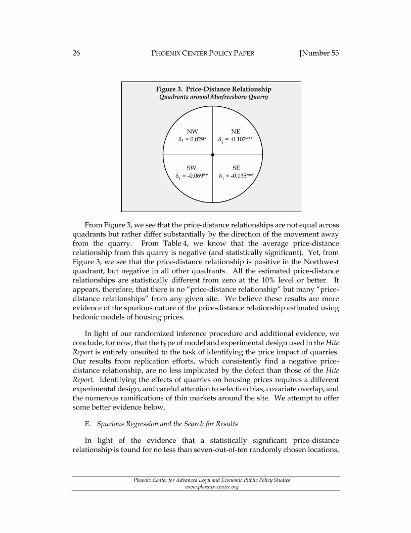
Another problem with estimating the price-distance relationship is that unlike square footage, distance from a quarry is not unidimensional but occurs on a coordinate plane. A house may be located to the east or to the west, to the north or to the south, of a quarry, and moving closer to or away from the town center, a university, a landfill, or any other site that may influence prices. To see this, we divide the transaction data near Murfreesboro into four quadrants around the quarry (northeast, northwest, southeast, and southwest) and estimate a price-distance relationship unique to each quadrant (using Eq. 2). Results are summarized in Figure 3.
26 PHOENIX CENTER POLICY PAPER [Number 53
Phoenix Center for Advanced Legal and Economic Public Policy Studies www.phoenix-center.org
From Figure 3, we see that the price-distance relationships are not equal across quadrants but rather differ substantially by the direction of the movement away from the quarry. From Table 4, we know that the average price-distance relationship from this quarry is negative (and statistically significant). Yet, from Figure 3, we see that the price-distance relationship is positive in the Northwest quadrant, but negative in all other quadrants. All the estimated price-distance relationships are statistically different from zero at the 10% level or better. It appears, therefore, that there is no “price-distance relationship” but many “price-distance relationships” from any given site. We believe these results are more evidence of the spurious nature of the price-distance relationship estimated using hedonic models of housing prices.
In light of our randomized inference procedure and additional evidence, we conclude, for now, that the type of model and experimental design used in the Hite Report is entirely unsuited to the task of identifying the price impact of quarries. Our results from replication efforts, which consistently find a negative price-distance relationship, are no less implicated by the defect than those of the Hite Report. Identifying the effects of quarries on housing prices requires a different experimental design, and careful attention to selection bias, covariate overlap, and the numerous ramifications of thin markets around the site. We attempt to offer some better evidence below.
E. Spurious Regression and the Search for Results
In light of the evidence that a statistically significant price-distance relationship is found for no less than seven-out-of-ten randomly chosen locations,
Figure 3. Price-Distance Relationship Quadrants around Murfreesboro Quarry
NW
1 = 0.029*
NE
1 = -0.102***
SW
1 = -0.069**
SE
1 = -0.135***
Winter 2018] QUARRY OPERATIONS AND PROPERTY VALUES 27
Phoenix Center for Advanced Legal and Economic Public Policy Studies www.phoenix-center.org
we conclude the Hite Report’s experimental design is incapable of quantifying the effect of quarries on house prices. The results from such models are spurious. Consequently, we expect that the price-distance relationship will be sometimes positive, sometimes negative, sometimes statistically significant and sometimes not for any given quarry. Statistical significance is the flip of a coin heavily weighted toward the rejection of the null hypothesis. Our analysis also shows that the choice of estimation method may alter the estimated coefficient and its significance, a common trait of spurious regression.
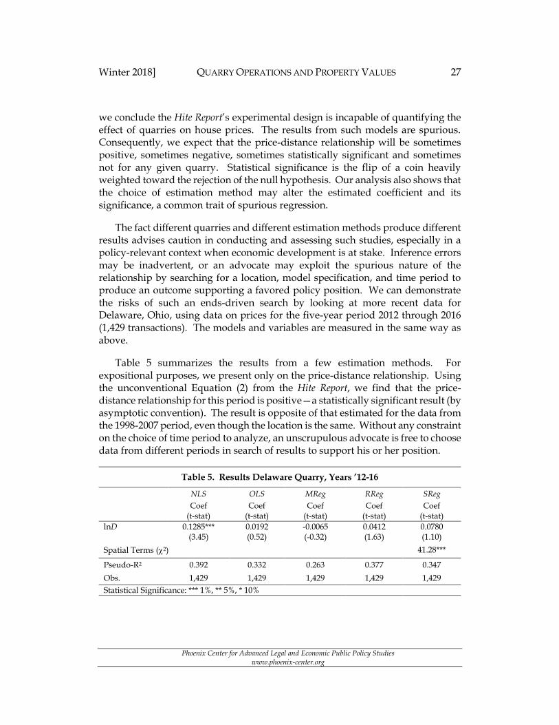
The fact different quarries and different estimation methods produce different results advises caution in conducting and assessing such studies, especially in a policy-relevant context when economic development is at stake. Inference errors may be inadvertent, or an advocate may exploit the spurious nature of the relationship by searching for a location, model specification, and time period to produce an outcome supporting a favored policy position. We can demonstrate the risks of such an ends-driven search by looking at more recent data for Delaware, Ohio, using data on prices for the five-year period 2012 through 2016 (1,429 transactions). The models and variables are measured in the same way as above.
Table 5 summarizes the results from a few estimation methods. For expositional purposes, we present only on the price-distance relationship. Using the unconventional Equation (2) from the Hite Report, we find that the price-distance relationship for this period is positive—a statistically significant result (by asymptotic convention). The result is opposite of that estimated for the data from the 1998-2007 period, even though the location is the same. Without any constraint on the choice of time period to analyze, an unscrupulous advocate is free to choose data from different periods in search of results to support his or her position.
Table 5. Results Delaware Quarry, Years ’12-16
NLS OLS MReg RReg SReg
Coef
(t-stat) Coef
(t-stat) Coef
(t-stat) Coef
(t-stat) Coef
(t-stat)
lnD 0.1285*** (3.45)
0.0192 (0.52)
-0.0065 (-0.32)
0.0412 (1.63)
0.0780 (1.10)
Spatial Terms (2) 41.28***
Pseudo-R2 0.392 0.332 0.263 0.377 0.347
Obs. 1,429 1,429 1,429 1,429 1,429
Statistical Significance: *** 1%, ** 5%, * 10%

28 PHOENIX CENTER POLICY PAPER [Number 53
Phoenix Center for Advanced Legal and Economic Public Policy Studies www.phoenix-center.org
Model selection and variable choice may also be used in an ends-drive search for results. As shown in Table 5, estimating Equation (3), a standard functional form for hedonic regressions, the positive coefficient is now a sixth the size of that estimated by Equation (2) and is no longer statistically different from zero at standard levels.37 Also, Median, Robust and Spatial Regression do not find statistically significant price-distance relationships. In fact, the only model that produces a statistically-significant positive effect is the non-standard regression equation used in the Hite Report. Moreover, if we replace the TOTR variable with the SQFT variable in the NLS model, the price-distance relationship shrinks to 0.02 (one-sixth the size) and the coefficient is no longer statistically significant. Again, a researcher may pick-and-choose model specification, along with time period analyzed and regressors, to obtain a desired result. Skepticism is warranted for any analysis of the price effects of quarries (and amenities or disamenities generally) absent robustness analysis across time and model specifications.
Table 6. Results Delaware Quarry, Years ’98-07 & ’12-16
NLS OLS MReg RReg SReg
Coef
(t-stat) Coef
(t-stat) Coef
(t-stat) Coef
(t-stat) Coef
(t-stat)
lnD 0.10028 (0.11)
-0.1361*** (-5.04)
-0.0963*** (-6.33)
-0.0501*** (-2.89)
-0.1059** (-2.10)
Spatial Terms (2) 41.28***
Pseudo-R2 0.302 0.262 0.219 0.288 0.151
Obs. 3,543 3,543 3,543 3,543 3,543
Statistical Significance: *** 1%, ** 5%, * 10%
As another check on robustness (or a lack thereof), we combine the data from 1998-2007 and 2012-2016, excluding those years when the housing market and economy generally were in turmoil (2008-2011). Results on the price-distance relationship are summarized in Table 6. Now, Equation (2) estimated by NLS reports a statistically insignificant (but positive) coefficient for the price-distance relationship. The other estimation methods, however, all confirm the negative and statistically significant relationship consistent with the results in Tables 1 and 3. It appears, therefore, whether or not quarries affect prices hinges on model selection and dates selected, which simply demonstrates the spurious nature of these sorts of experiments. Plainly, care must be given to model selection, and robustness analysis should be thorough and explicit. And, in light of the randomized
37 The Box-Cox test indicates a preference for the transformation (2 = 40.7).

Winter 2018] QUARRY OPERATIONS AND PROPERTY VALUES 29
Phoenix Center for Advanced Legal and Economic Public Policy Studies www.phoenix-center.org
inference and quadrant analysis above, the utility of the price-distance relationship for quantifying the effects of quarries and disamenities should be regarded as defective, at least until further research demonstrates otherwise.
The analyses presented here, we believe, offers compelling evidence that the Hite Report’s experimental design is a flimsy method, easily manipulated to produce nearly any desired result through the selection of location, model specification, estimation technique, and the time period analyzed. The Hite Report’s findings cannot be reliably replicated and conflicting results are readily obtained. The spurious nature of the price-distance relationship from such experiments is clearly demonstrated, and the defective approach allows for nearly any result imaginable. Using data long after a quarry opens poses no limits on the selection of time period, enhancing the risk of the exploitation of spurious regression for economic and political advantage.
IV. A Difference-in-Difference Approach
As detailed above, to quantify the effect of a quarry on home prices the researcher ideally needs pricing data both before and after quarry operations begin.38 With this data, statistical analysis can determine how the relationship between price and distance from the quarry changes after the quarry opens, thus quantifying, under some well-known assumptions, a plausible causal effect.
There are some potential shortcomings with a simple before-and-after analysis, however. New quarries take years to get approval and normally we expect equity prices to reflect new information quickly, so price effects may precede that event. In this section, we offer two before-and-after analyses of the effect of a quarry on home prices. First, we evaluate pricing activity around the Vulcan quarry in Gurley, Alabama, which began operations in 2013. Gurley is a rural area not far from the city of Huntsville, Alabama. Consistent with the analysis above, we use the general format of the Hite Report (and several
38 Another possible identification strategy involves exploiting policy experiments with respect to residential distance from a quarry. For example, if some states required houses to be a certain distance away from a quarry while other states did not, then a credible counter-factual could be constructed allowing the researcher to estimate the effect of quarry distance on home prices. A regression discontinuity design could be used to identify the price-distance relationship if regulations required potential home buyers to be informed of the quarry for homes within a certain distance. Homes just inside and just outside this cut-point would could be used as treatment and control units to identify the causal price-distance relationship.
(Footnote Continued. . . .)

30 PHOENIX CENTER POLICY PAPER [Number 53
Phoenix Center for Advanced Legal and Economic Public Policy Studies www.phoenix-center.org
alternatives) to test for a change in the price-distance relationship after the quarry opens.
Second, we evaluate the price effects of the contested Austin Quarry in Madera, California, which was approved in 2016.39 Located in the southwest corner of the intersection of Highway 41 and Highway 145, the site is proximate to two subdivisions, one located on Highway 145 and the other on Highway 41. Thus, not only are the subdivisions proximate to the quarry, but both are expected to deal regularly with the quarry’s traffic flow. Though first proposed in 2010, media coverage and public protest did not begin until 2013, at which time the new quarry might be expected to affect home prices through an announcement effect.40 A control group is chosen using CEM from homes sales in subdivisions not too far from the quarry site but beyond the range of influence. We find no statistically significant effect of the quarry in either model, though in both cases the estimated coefficients indicate, if anything, the quarry raises property values.
A. The Empirical Model
For these analyses, we employ the standard regression model for the DiD estimator. Using a log-linear form common to hedonic regressions, the regression equation is,
k
it i i j j i itj
p T N N X0 0 ,2
ln
, (4)
where T is dummy variable equal to 1.0 after the treatment and Ni is a dummy variable for homes near the quarry site (or a continuous measure of distance from
the quarry). The estimated coefficient 0 measures the difference in average sale prices for homes near the quarry (or the effect of distance from it) prior to the treatment. After the treatment, the difference in price between homes near and far
from the quarry is + 0. The difference between the two effects is , which is the
DiD estimator, as defined in Equation (1), or = 1 – 0. The t-test on the coefficient
39 J. Rieping, Controversial Quarry Up for Vote, MADERA TRIBUTE (July 16, 2016) (available at: http://www.maderatribune.com/single-post/2016/07/16/Controversial-quarry-up-for-vote); M.E. Smith, Austin Quarry Approved in 3-2 Vote, SIERRA STAR (July 20, 2016) (available at: http://www.sierrastar.com/latest-news/article90713132.html).
40 Lexus-Nexus search conducted on February 20, 2018. B. Wilkinson, Concerns Over Truck Traffic on Road, SIERRA STAR (February 21, 2013).

Winter 2018] QUARRY OPERATIONS AND PROPERTY VALUES 31
Phoenix Center for Advanced Legal and Economic Public Policy Studies www.phoenix-center.org
is, therefore, a direct test of the statistical significance of the effect of a quarry on home prices.
As an alternative, we estimate,
k
it i j j i t itj
p T N X0 ,2
ln
, (5)
where the continuous DATE variable is replaced with year fixed effects (t), which is a somewhat standard treatment of time in the DiD regression. Due to
collinearity with the fixed effects, the 0N term is no longer included in the
regression, but the interpretation of is unchanged.
For consistency with the earlier analysis, we also estimate the model specification of the Hite Report, adding as a regressor the interaction of a treatment dummy variable for years 2013 and later (T). The regression model is,
k
it i i j j i itj
p D T D X0 0 ,2
exp( ln ln )
, (6)
where the variables are defined the same way as the Murfreesboro analysis (i.e.,
total rooms is replaced with square footage). The coefficient 0 quantifies the price-distance relationship prior to the initiation of quarry operations in 2013. Starting
in 2013, the price-distance relationship is measured by 0 + = 1, where measures the change in the slope of the price-distance relationship. If the quarry
reduces home values near the quarry, then should be positive and statistically significant. Equation (6) is estimated by NLS.
B. Vulcan Quarry in Gurley, Alabama
As with the earlier analysis, data is obtained on home sales within a five-mile radius of the quarry location in Gurley, Alabama. The quarry began operations in 2013, and our data spans 2005 through portions of 2017. The sample includes 593 transactions, but we note only 83 are for sales prior to 2013.41 Since there is no “city
41 The low samples are likely the consequence of the rural nature of the market and data collection in such areas. We cannot exclude the possibility the sample is peculiar in some respect.

32 PHOENIX CENTER POLICY PAPER [Number 53
Phoenix Center for Advanced Legal and Economic Public Policy Studies www.phoenix-center.org
center” in the area, the DCC variable is measured as the distance from the WalMart Supercenter in the nearby town of Big Cove.
Table 7. Regression Results and Descriptive Statistics Vulcan Quarry in Gurley, Alabama
NLS-Eq. 6 Coef
(t-stat)
OLS-Eq. 4 Coef
(t-stat)
OLS-Eq. 5 Coef
(t-stat)
Mean (St. Dev)
lnD 0.0876 (0.97)
0.2723*** (3.64)
0.3679** (2.20)
3.445 (0.987)
TlnD -0.1205** (-2.41)
-0.0543 (-1.07)
-0.1587 (-0.88)
2.936 (1.50)
DATE 0.0162* (1.67)
0.0191* (1.85)
… 2014.1 (2.30)
DDC -0.0456*** (-5.85)
-0.0529*** (-5.99)
-0.0512*** (-5.80)
4.484 (2.27)
H2L -1.2185 (-0.79)
-0.2457 (-0.11)
0.1868 (0.08)
0.063 (0.029)
BATH 0.1752*** (6.92)
0.2672*** (8.84)
0.2655*** (8.71)
2.875 (0.932)
SQFT 2.2E-04*** (5.97)
2.0E-04*** (3.22)
1.9E-04*** (3.11)
2,870.3 (1,139.8)
Constant -27.99 (-1.43)
-27.57 (-1.32)
10.61*** (36.57)
…
t No No Yes …
Pseudo-R2 0.641 0.602 0.608 …
Obs. 593 593 593 593
Statistical Significance: *** 1%, ** 5%, * 10%
Results are summarized in Table 7.42 Many of the coefficients are statistically significant and similar to those estimated using the Murfreesboro data. First, for Equation (6) estimated by NLS, we find that housing prices rise as distance from the quarry increases (the coefficient on lnD is positive), but this positive effect is observed prior to the beginning of quarry operations. After the quarry opens, the positive (though statistically insignificant) price-distance relationship is
attenuated; the estimated coefficient is -0.103 and the null hypothesis of “no effect” for the DiD estimator is rejected at the 5% level. Prior to 2013, the price-
42 Since we do not observe large differences in the characteristics of homes near to and far from the quarry, we do not apply CEM.
Winter 2018] QUARRY OPERATIONS AND PROPERTY VALUES 33
Phoenix Center for Advanced Legal and Economic Public Policy Studies www.phoenix-center.org
distance elasticity is 0.088 (0), but after 2013 it is -0.033 (1), a small effect that is statistically indistinguishable from zero (F-stat = 0.16, prob = 0.69).
Turning to Equation (4), the price-distance relationship is again positive (and much larger than with NLS) but is now statistically significant prior to the
beginning of quarry operations. The coefficient is -0.054, which while negative is no longer statistically different from zero at standard levels. The positive price-distance relationship is attenuated after the quarry began operating, but not to a statistically significant degree. The results are similar for Equation (5). Though not summarized in the table, we note that for MReg and RReg neither of the quarry-distance coefficients is statistically different from zero. The SReg results, also not presented in the table, are not wholly unlike the OLS estimates of Equation
(4); the coefficient 0 is positive (0.331, t = 4.45) and statistically significant, but the
coefficient is negative (-0.055, t = 0.98) and not statistically different from zero.
The lack of robustness to specification leads us to conclude that the most likely effect of the quarry is no effect at all. Also, we acknowledge that the defects in the Hite Report’s empirical strategy is as relevant here as before: our randomized
inference simulation computes a rejection rate on 0 of 65% and for of 67% (at a nominal 10% significance level). While we recognize the limitations of the data and the methods, on whole the results are entirely at odds with the claim that quarries reduce housing prices. If anything, the effect is the opposite.
C. Austin Quarry in Madera County, California
Quarry sites often take years for approval. Our model of the Gurley quarry presumed that prices do not reflect the quarry operations until after the quarry is operational. A reasonable argument may be made, however, that home prices might adjust before the quarry opens when the local population becomes aware of the future quarry site. We consider that possibility now.
The Austin Quarry in Madera, California, was approved in September 2016 despite a substantial NIMBY effort.43 A search of news outlets reveals that public attention to proposed quarry initiated in early 2013 and was very active is
43 M. Smith, Supervisors Approve Austin Quarry 3-2, SIERRA STAR (September 12, 2016) (available at: http://www.sierrastar.com/news/local/article101492412.html).
(Footnote Continued. . . .)

34 PHOENIX CENTER POLICY PAPER [Number 53
Phoenix Center for Advanced Legal and Economic Public Policy Studies www.phoenix-center.org
subsequent years.44 Thus, we define the treatment dummy T as having values of one in years after 2013 (and also consider other years). Data is collected for the ten years preceding the treatment date, so the data spans 2007 through 2016.
The Austin Quarry site is well outside of town, but there are two subdivisions proximate (less than three miles) to the site: Bonadelle Racheros-Madera Ranchos and Bonadelle Rancheros Nine. Both subdivisions abut the major highways (Highways 41 and 145) servicing the quarry site. If any homes are to be affected by the quarry, then these are the most likely candidates, and they represent our treatment group. The dummy variable N takes a value of 1 for these subdivisions (zero otherwise). Visual inspection of the area points to a number of subdivisions in the vicinity that are neither on the major highways serving the site nor within ten miles of the site: Madera Estates, Madera Country Club, Lake Madera Country Club, Chuk Chanse, Valley Lake Ranchos, Madera Acres, Madera Knolls, and Madera Highlands. A control group will be selected from home sales in these subdivisions.
Estimation of the DiD estimator employs Equation (5). Regressors include the age of the home at the sale data (AGE), square footage (SQFT), the number of bedrooms (BED) and bathrooms (BATH), a dummy variable indicating whether the home a two story home (STRY), a dummy variable indicating the presence of a fireplace (FIRE), a dummy variable indicating whether the home has a swimming pool (POOL). Year fixed effects are included.
44 B. Wilkinson, Concerns Over Truck Traffic on Road, SIERRA STAR (February 32, 2013); G. Smith, Economic Costs and Benefits of the Proposed Austin Quarry in Madera County (October 23, 2014) (available at: http://www.noaustinquarry.org/wp-content/uploads/2016/08/Austin-Quarry-Economics-Report.pdf); M.E. Smith, Progress Continues on Austin Quarry, SIERRA STAR (February 10, 2016) (available at: http://www.sierrastar.com/news/article87816032.html); B. Wilkinson, Group Opposes Proposed Rock Quarry, SIERRA STAR (November 12, 2014) (available at: http://www.sierrastar.com/news/article87802492.html); D. Joseph, Quarry Issues Need to be Addressed, SIERRA STAR (December 3, 2014) (available at: http://www.sierrastar.com/opinion/article87803072.html).

Winter 2018] QUARRY OPERATIONS AND PROPERTY VALUES 35
Phoenix Center for Advanced Legal and Economic Public Policy Studies www.phoenix-center.org
Table 8. Descriptive Statistics Austin Quarry in Madera County, California
Variable ALL
Mean (St.Dev)
N=0 Mean
(St.Dev)
N=1 Mean
(St.Dev) Stan. Diff.
AGE 16.13 (12.16)
16.50 (12.22)
15.21 (11.95)
0.075
SQFT 1811.6 (522.7)
1706.7 (490.6)
2072.9 (509.5)
0.518*
BED 3.32 (0.59)
3.27 (0.54)
3.43 (0.70)
0.179
BATH 1.99 (0.68)
1.83 (0.66)
2.38 (0.56)
0.639*
STRY 0.024 (0.15)
0.016 (0.12)
0.043 (0.20)
0.115
FIRE 0.632 (0.48)
0.730 (0.44)
0.390 (0.49)
0.515*
POOL 0.068 (0.25)
0.033 (0.17)
0.159 (0.36)
0.311*
Price 215.4 195.0 266.3
Price/SQFT 120.8 116.4 131.9
Obs. 887 633 254
Descriptive statistics for the treatment and control pool are provided in Table 8. The homes are similar in some respects, but large standardized differences (> 0.25) are found for square footage, the number of bathrooms, and the presence of a fireplace or pool.45 CEM based on SQFT, BATH, FIRE, and POOL reduces the standardized differences to acceptable levels for all the regressors. We are able to match 229 of 254 homes in the treated group to 450 of 633 homes in the control pool, for an estimation sample of 679 home sales.
45 Imbens and Wooldridge, supra n. 8.

36 PHOENIX CENTER POLICY PAPER [Number 53
Phoenix Center for Advanced Legal and Economic Public Policy Studies www.phoenix-center.org
Table 9. Regression Results and Descriptive Statistics Austin Quarry in Madera County, California
OLS Coef
(t-stat)
CEM-OLS Coef
(t-stat)
CEM-MReg Coef
(t-stat)
SReg Coef
(t-stat)
N (0) 0.1166** (2.47)
0.1277** (2.08)
0.1194*** (4.99)
0.1913** (2.11)
TN () 0.1663*** (2.95)
0.1005 (1.21)
0.1161*** (3.14)
0.0878 (1.32)
AGE 0.0017 (1.20)
0.0087*** (3.47)
-0.0003 (-0.35)
-0.0055* (-0.35)
SQFT 1.7E-04*** (3.40)
1.3E-04** (2.05)
3.0E-04*** (12.68)
2.0 E-04*** (4.39)
BED 0.0349 (0.90)
0.01205*** (2.63)
0.0450** (2.49)
-0.0542 (1.54)
BATH 0.0288 (1.08)
-0.0439 (-0.60)
-0.0777*** (-2.60)
-0.0218 (-0.61)
STRY -0.0878 (-0.70)
-0.0408 (-0.33)
0.0043 (0.05)
-0.1378 (-1.29)
FIRE 0.0770** (2.43)
0.0650* (1.73)
0.0422*** (2.94)
0.0305 (0.88)
POOL 0.1833*** (3.71)
0.1577*** (4.03)
0.0853*** (3.68)
0.2346*** (3.63)
Constant 11.21*** (98.08)
10.92*** (70.30)
11.35*** (20.67)
11.62*** (83.17)
t Yes Yes Yes Yes
Spatial Terms (2) 27.17***
Pseudo-R2 0.482 0.491 0.361 0.186
Obs. 887 679 679 887
Statistical Significance: *** 1%, ** 5%, * 10%
Regression results are summarized in Table 9. For comparison purposes and to illustrate the important effects of covariate balance, estimates for both the full and CEM-weighted samples are provided. The models fit the data well for both samples. For the full sample, which we caution does not rely on balanced data,
the estimated 0 coefficient (0.117) indicates that prices in the treated group were
about 12% higher [exp(0) - 1] in the pre-treatment period. After the treatment, the
prices were even higher ( = 0.166), a statistically significant result of about an 18% increase. The remaining coefficients are sensibly sized and many are statistically different from zero. A swimming pool, for instance, raises price by about $38,000.
Turning to the CEM-weighted model, the price difference before the treatment
is a bit larger (0 = 0.128), and the difference is statistically significant at standard

Winter 2018] QUARRY OPERATIONS AND PROPERTY VALUES 37
Phoenix Center for Advanced Legal and Economic Public Policy Studies www.phoenix-center.org
levels. As in the full sample, the DiD estimator is positive (0.100), but now it is not statistically significant. For the balanced sample, we cannot reject the null hypothesis that the quarry’s announcement effect is zero, though the coefficient is relatively large and the t-statistic is much larger than 1.00. In contrast, for the CEM-weighted MReg, prices are higher in the treated area during both the pre-treatment and treatment period, and both coefficients are statistically different from zero at better than the 1% level.
In the final column of Table 9, we summarize the results from SReg using the full sample. The spatial terms are statistically significant at the 1% level. The results are comparable to the others. Prices are higher in the treated area before the treatment, but we do not see a statistically significant change is seen after the
treatment. The DiD estimator is positive and relatively large (0.09), but statistically significant only at the 20% level.
Table 10. Regression Results, Annual Treatment Effect Austin Quarry in Madera County, California
2013 Coef
(t-stat)
2014 Coef
(t-stat)
2015 Coef
(t-stat)
2016 Coef
(t-stat)
TN () 0.2721*** (2.65)
0.0018 (0.01)
0.0322 (0.42)
0.3949 (1.41)
Statistical Significance: *** 1%, ** 5%, * 10%
Finally, we can estimate the coefficient for each year beginning with our chosen treatment date (2013), thereby assessing whether that choice is influencing the estimate.46 The results by year are summarized in Table 10. Large positive coefficients are observed in years 2013 and 2016 (the latter close to being statistically significant), and smaller positive coefficients for the other years. These results are consistent with those reported in Table 9.
Notably, we do not estimate a price-distance relationship in these equations. Distance from the quarry site is not a regressor. Unlike the distance-based model, the rejection rates for randomized inference (assigning the homes in the treatment group randomly from those in the sample) are very close to the nominal level of the test (11% rejection rate versus 10% nominal test level). The statistical reliability
46 The coefficients are year specific and do not quantify the average after the treatment year, as do the results from Table 9.

38 PHOENIX CENTER POLICY PAPER [Number 53
Phoenix Center for Advanced Legal and Economic Public Policy Studies www.phoenix-center.org
of this approach is much superior to the price-distance approach used in the Hite Report.
Taken together, we conclude from these results indicate that the effect of the quarry may very well be zero, at least in the form of an announcement effect. If there is any effect, it is positive. Whether or not the quarry will affect prices, either positively or negatively, after operations begin (assuming they do) is unknowable at this time. In light of the evidence presented here and in prior research, the expectation must be that there will be little to no effect on home prices and, if anything, that effect may be positive.
V. Conclusions
We estimate the effect of rock quarries on home prices with data from four quarry locations across the United States, a wide range of econometric specifications and robustness checks, and a variety of temporal circumstances from the lead-up to quarry installation to subsequent operational periods. We find no compelling statistical evidence that either the anticipation of, or the ongoing operation of, rock quarries negatively impact home prices. While our study extends the literature on estimating the effects of “disamenities,” primarily as a critique of existing methods, the empirical problem is difficult and likely requires advanced research methods beyond what we provide here. The primary obstacle to estimating these effects is the lack of data and that lack of data is actually driven by the quarry site selection process, which limits our ability to infer a causal relationship. Thin markets and a subsequent lack of sales data are a serious problem since quarries are today (and typically in the past) located, by design, away from residential density.
Our study highlights a number of shortcomings in the empirical methodologies generally used to estimate the effect of disamenities on real estate prices. First and foremost, the vast majority of studies do not (or even attempt to) identify the causal effect of disamenities. That is, existing studies are naïve as to the empirical conditions necessary to identify a causal relationship and do not establish credible strategies to estimate the counter-factual outcome—i.e., how the real estate around quarries would have looked, on average, without a landfill or other disamenity. To evaluate the credibility of existing studies and their methodologies, we first employ permutation tests to examine whether or not the existing methodologies yield higher than expected rejection rates of the null hypothesis. We accomplish this by randomly assigning a location in our sample space with a “disamenity” (i.e., a placebo quarry) and then estimate the effect on surrounding home prices. The null hypothesis of “no effect” of the placebo

Winter 2018] QUARRY OPERATIONS AND PROPERTY VALUES 39
Phoenix Center for Advanced Legal and Economic Public Policy Studies www.phoenix-center.org
quarries is rejected in no less than 7 out of 10 simulations, and at a rate as high as 9 out of 10 simulations.
In an attempt to produce a meaningful counter-factual we employ a difference-in-differences estimation strategy which exploits the timing and placement of a quarry. We use this strategy in two different contexts: (1) before and after operations of a quarry in Gurley, Alabama; and (2) before and after local debate (and subsequent approval) of a quarry in Madera County, California. The first exercise estimates the effect of quarry operations on home prices and the second exercise estimates the anticipatory effect of a quarry on home prices. Neither exercise yields evidence of a negative impact on home prices. Given a number of data concerns and model limitations (since our interest is primarily in replication), further research is advised.
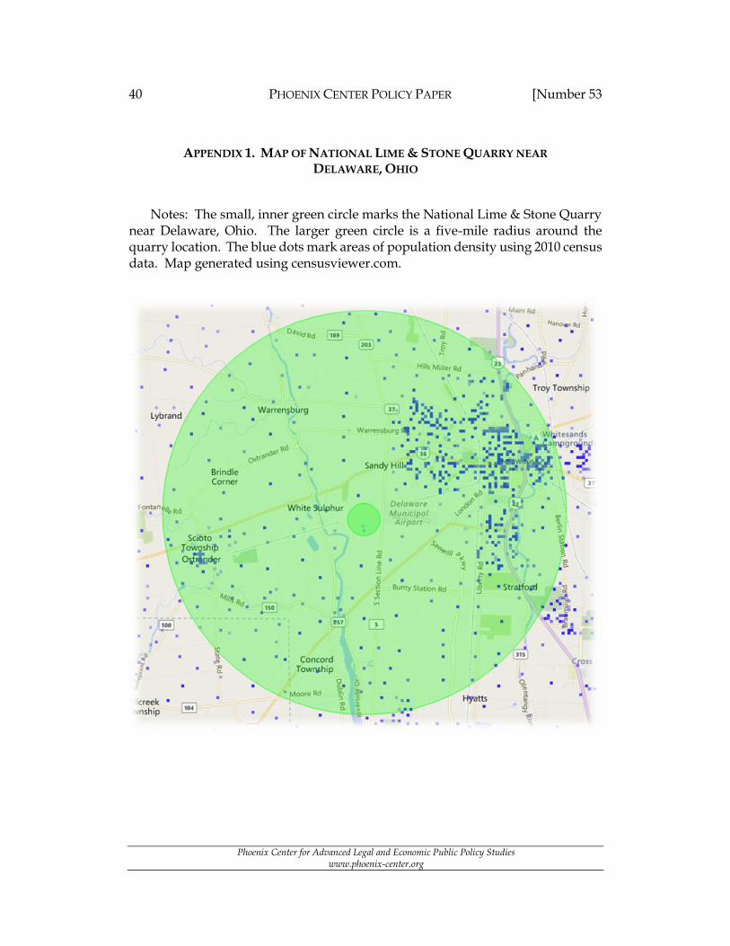
40 PHOENIX CENTER POLICY PAPER [Number 53
Phoenix Center for Advanced Legal and Economic Public Policy Studies www.phoenix-center.org
APPENDIX 1. MAP OF NATIONAL LIME & STONE QUARRY NEAR DELAWARE, OHIO
Notes: The small, inner green circle marks the National Lime & Stone Quarry near Delaware, Ohio. The larger green circle is a five-mile radius around the quarry location. The blue dots mark areas of population density using 2010 census data. Map generated using censusviewer.com.
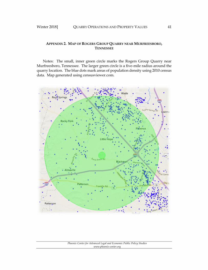
Winter 2018] QUARRY OPERATIONS AND PROPERTY VALUES 41
Phoenix Center for Advanced Legal and Economic Public Policy Studies www.phoenix-center.org
APPENDIX 2. MAP OF ROGERS GROUP QUARRY NEAR MURFREESBORO, TENNESSEE
Notes: The small, inner green circle marks the Rogers Group Quarry near Murfreesboro, Tennessee. The larger green circle is a five-mile radius around the quarry location. The blue dots mark areas of population density using 2010 census data. Map generated using censusviewer.com.

42 PHOENIX CENTER POLICY PAPER [Number 53
Phoenix Center for Advanced Legal and Economic Public Policy Studies www.phoenix-center.org
APPENDIX 3. CENSUS BLOCK POPULATION GROWTH NEAR ROGERS GROUP
QUARRY NEAR MURFREESBORO, TENNESSEE
Notes: Figures 3A-3C demonstrate population movements for Rutherford County, TN, with emphasis on the Rogers Group quarry. Population is measured using U.S. Census Bureau population data for years 2000, 2010, and 2016. Darker blues imply greater population.
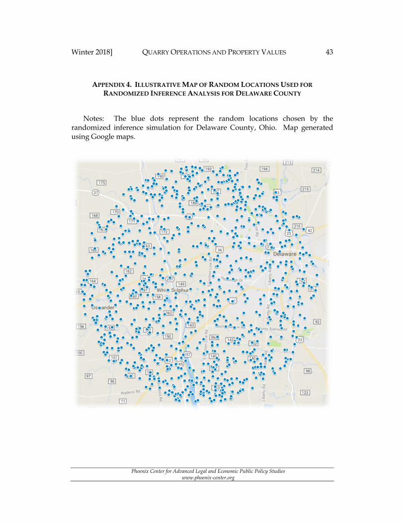
Winter 2018] QUARRY OPERATIONS AND PROPERTY VALUES 43
Phoenix Center for Advanced Legal and Economic Public Policy Studies www.phoenix-center.org
APPENDIX 4. ILLUSTRATIVE MAP OF RANDOM LOCATIONS USED FOR
RANDOMIZED INFERENCE ANALYSIS FOR DELAWARE COUNTY
Notes: The blue dots represent the random locations chosen by the randomized inference simulation for Delaware County, Ohio. Map generated using Google maps.
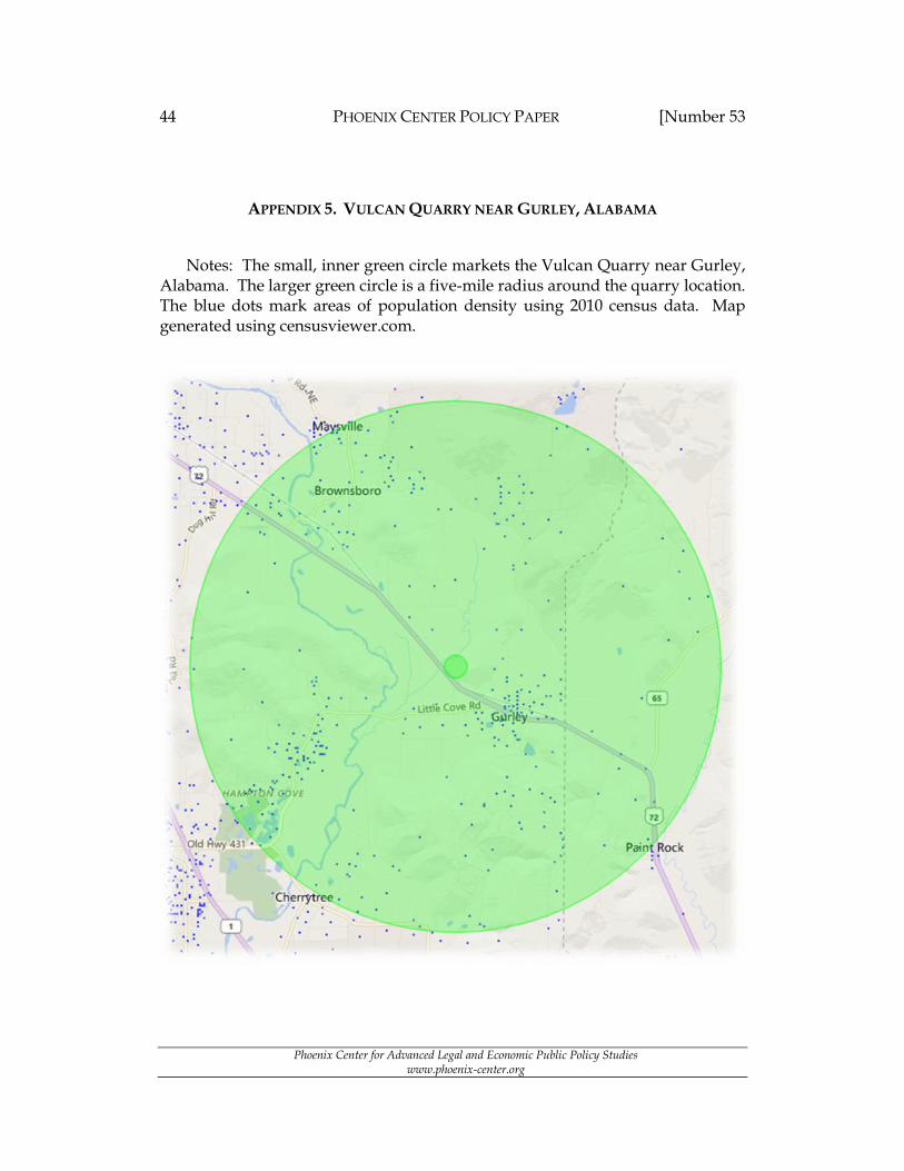
44 PHOENIX CENTER POLICY PAPER [Number 53
Phoenix Center for Advanced Legal and Economic Public Policy Studies www.phoenix-center.org
APPENDIX 5. VULCAN QUARRY NEAR GURLEY, ALABAMA
Notes: The small, inner green circle markets the Vulcan Quarry near Gurley, Alabama. The larger green circle is a five-mile radius around the quarry location. The blue dots mark areas of population density using 2010 census data. Map generated using censusviewer.com.

Winter 2018] QUARRY OPERATIONS AND PROPERTY VALUES 45
Phoenix Center for Advanced Legal and Economic Public Policy Studies www.phoenix-center.org
APPENDIX 6. MAP OF AUSTIN QUARRY SITE IN MADERA COUNTY, CALIFORNIA
Notes: The green circle marks the site of the proposed Austin Quarry in Madera County, California. The immediate two areas of population to the South and West of the quarry site—marked in green rectangles—are the “treated” areas. The blue dots mark areas of population density using 2010 census data. The control group is chosen from areas further west and north of Highway 145 toward Madera. Map generated using censusviewer.com.