quasivelocities and symmetries in nonholonomic systems
TRANSCRIPT

Quasivelocities and Symmetries in Nonholonomic
Systems
Anthony M. BlochDepartment of Mathematics
University of MichiganAnn Arbor, MI 48109
Jerrold E. MarsdenControl and Dynamical Systems
California Institute of Technology 107-81Pasadena, CA [email protected]
Dmitry V. Zenkov∗
Department of MathematicsNorth Carolina State University
Raleigh, NC [email protected]
Keywords: Hamel equations, momentum, symmetryAMS Subject Classification: 70F25, 37J60, 70H33
Abstract
This paper is concerned with the theory of quasivelocities for nonholonomicsystems. The equations of nonholonomic mechanics are derived using the La-grange–d’Alembert principle written in an arbitrary configuration-dependentframe. The paper also shows how quasivelocities may be used in the formu-lation of nonholonomic systems with symmetry. In particular, the use of qua-sivelocities in the analysis of symmetry that leads to unusual momentum con-servation laws is investigated, as is the applications of these conservation lawsand discrete symmetries to the qualitative analysis of nonholonomic dynamics.The relationship between asymptotic dynamics and discrete symmetries of thesystem is also elucidated.
∗Corresponding author
1

1 Introduction 2
1 Introduction
Quasivelocities are the velocities of a mechanical system expressed relative to aconfiguration-dependent frame. The mathematical underpinnings of quasivelocitiesin texts such as Neimark and Fufaev [1972] and Greenwood [2003] have not beenas developed as is desirable, although their usefulness was clearly demonstrated.The additional clarity provided by the present paper should expand the scope ofapplications and uses of this important concept.
The goal of this paper is to develop the use of quasivelocities in the dynamicsof nonholonomic systems with symmetry. Key forms of the equations of dynam-ics including the Hamel equations and the Euler–Lagrange–Poincare equations arederived, and their relationship to quasivelocities is spelled out. The equations ofmotion for nonholonomic systems are obtained, and conditions under which an ap-propriate choice of frame evokes otherwise hidden momentum conservation laws arefound. The resulting formalism is utilized in the analysis of the dynamics of someinstructive nonholonomic systems including the Chaplygin sleigh and the sleigh cou-pled to an oscillator.
Said from a slightly different perspective, quasivelocities are the components ofa mechanical system’s velocity relative to a set of vector fields that span the fibersof the tangent bundle of the configuration space. These vector fields need not beassociated with (local) configuration coordinates, so in fact, this paper does notmention “quasicoordinates”, a vacuous concept that has led to some confusion inthe literature. A good example of quasivelocities is the set of components of thebody angular velocity of a rigid body rotating about a fixed point.
One of the reasons for using quasivelocities is that the Euler–Lagrange equationswritten in generalized coordinates are not always effective for analyzing the dynamicsof a mechanical system of interest. For example, it is difficult to study the motion ofthe Euler top if the Euler–Lagrange equations (either intrinsically or in generalizedcoordinates) are used to represent the dynamics. On the other hand, the use ofthe angular velocity components relative to a body frame pioneered by Euler [1752]results in a much simpler representation of dynamics. Euler’s approach was furtherdeveloped by Lagrange [1788] for reasonably general Lagrangians on the rotationgroup and by Poincare [1901] for arbitrary Lie groups (see Marsden and Ratiu [1999]for details and history). Other examples include the use of velocity and angularvelocity components relative to a moving frame in the study of dynamics of a rigidbody moving on a surface as discussed in Routh [1860] and Markeev [1992].
Quasivelocities used in Lagrange [1788] and Poincare [1901] are associated witha group action. Hamel [1904] obtained the equations of motion in terms of quasive-locities that were unrelated to a group action on the configuration space. The Hamelequations include both the Euler–Lagrange and Euler–Poincare equations (for therigid body for example) as special cases.
This paper derives the Hamel equations from a variational point of view; thatis, it develops the form of the principle of critical action that is equivalent to theHamel equations. It is then shown how the quasivelocity approach is useful in thetreatment of nonholonomic systems with symmetry. In particular, the selection of

1 Introduction 3
suitable quasivelocies appropriate to the presence of discrete symmetries is developedalong with the application to the qualitative analysis of dynamics.
Nonholonomic systems with symmetry are studied in Bloch, Krishnaprasad,Marsden, and Murray [1996] and improved in related references, such as Cendra,Marsden, and Ratiu [2001a]. According to these papers, symmetry and constraintsdefine certain subbundles of the tangent bundle of the configuration manifold. Aswill be shown, it is beneficial to select frames that respect this subbundle structure,that is, frames obtained by concatenation of the bases of these subbundles. Theseframes elucidate the momentum equations and conservation laws in the system.
The dynamics of a nonholonomic system with symmetry on the subbundle whosefibers are tangent to the group orbits is governed by the momentum equation, anequation that was introduced in Bloch, Krishnaprasad, Marsden, and Murray [1996].As shown in Zenkov, Bloch, and Marsden [1998], the momentum equation is impor-tant in the energy-based analysis of stability of relative equilibria. In the absence ofexternal dissipation these relative equilibria are often orbitally asymptotically sta-ble in certain directions in the phase system. Related work on this subject includesRuina [1998], Bloch [2000], and Zenkov and Bloch [2003]. Additional backgroundand references may be found in Bloch [2003].
The definition of nonholonomic momentum and the derivation of the momentumequation in Bloch, Krishnaprasad, Marsden, and Murray [1996] relies on the formal-ism that uses spatial frames. This paper utilizes the flexibility of Hamel equationsand gives a derivation of the momentum equation in a body frame. In a sense, this isa more natural and straightforward approach since the spatial momentum is almostnever conserved in the nonholonomic setting.
The structure of the momentum equation is then used to find conditions underwhich one has frames that reveal otherwise hidden momentum conservation laws. Insome instances the construction of such a frame is algorithmic, although it often leadsto implicitly defined frames. In other instances a frame that depends on the groupvariables in a nontrivial way is necessary for uncovering momentum conservationlaws. An example of this latter case is the unbalanced Chaplygin sleigh.
It is not unusual to have points in the configuration space where the fields thatdefine these frames become linearly dependent. This feature is studied and itsutilization in the qualitative analysis of a system’s dynamics is discussed.
The paper is organized as follows. In §2 we review the Hamel equations. In§3 nonholonomic systems are briefly discussed and their dynamics is written in theform of constrained Hamel equations. In §4 the equations of motion of systemswith symmetry are derived using quasivelocities. This derivation differs from thatin Bloch, Krishnaprasad, Marsden, and Murray [1996] and in Cendra, Marsden,and Ratiu [2001a] in interesting ways and illustrates the influence of symmetry onthe structure of qusivelocities. The nonholonomic momentum conservation and thecorresponding frame selection are discussed. In §5 nonholonomic systems on Liegroups and their measure-preserving properties are treated. Examples are given in§6, where, in particular, momentum conservation in the unbalanced Chaplygin sleighand integrability of the coupled sleigh-oscillator system are established. Finally, thethe asymptotic behavior of momentum conservation laws is studied.

2 Lagrangian Mechanics 4
2 Lagrangian Mechanics
In this section we review the equations of motion for holonomic systems from theLagrangian viewpoint.
2.1 Equations of Motion
The Euler–Lagrange Equations. A Lagrangian mechanical system is specifiedby a smooth manifold Q called the configuration space and a function L : TQ→ Rcalled the Lagrangian. In many cases, the Lagrangian is the kinetic minus potentialenergy of the system with the kinetic energy defined by a Riemannian metric on theconfiguration manifold and the potential energy being a smooth function on Q. Ifnecessary, non-conservative forces can be introduced (e.g., gyroscopic forces that arerepresented by terms in L that are linear in the velocity), but this is not discussedin this paper.
In local coordinates q = (q1, . . . , qn) on the configuration space Q we writeL = L(q, q). The dynamics is given by the Euler–Lagrange equations
d
dt
∂L
∂qi=∂L
∂qi, i = 1, . . . , n. (2.1)
These equations were originally derived by Lagrange in 1788 by requiring thatsimple force balance F = ma be covariant, i.e. expressible in arbitrary general-ized coordinates. A variational derivation of the Euler–Lagrange equations, namelyHamilton’s principle (also called the principle of critical action), came later in thework of Hamilton in 1834/35. For more details see Marsden and Ratiu [1999] andBloch [2003].
The Hamel Equations. In this paragraph we introduce the Hamel’s equations.In §2.3 we derive these equations from a global variational principle, generalizingthe reduced principle of critical action for systems with symmetry.
In many cases the Lagrangian and the equations of motion have a simpler struc-ture when written using so-called noncommuting variables. An example of such asystem is the rigid body. Below we develop a general approach that allows one toobtain the Euler–Lagrange equations in such noncommuting variables.
Let q = (q1, . . . , qn) be local coordinates on the configuration space Q and ui ∈TQ, i = 1, . . . , n, be smooth independent local vector fields defined in the the samecoordinate neighborhood.1 The components of ui relative to the basis ∂/∂qj will bedenoted ψji ; that is,
ui(q) = ψji (q)∂
∂qj, i, j = 1, . . . , n, (2.2)
where a sum on j is understood.1In certain cases, some or all of ui can be chosen to be global vector fields on Q.

2.2 The Virtual Displacement Principle 5
Let v = (v1, . . . , vn) ∈ Rn be the components of the velocity vector q ∈ TQrelative to the basis u1, . . . , un, i.e.,
q = viui(q); (2.3)
thenl(q, v) := L(q, viui(q)) (2.4)
is the Lagrangian of the system written in the local coordinates (q, v) on the tangentbundle TQ. The coordinates (q, v) are the Lagrangian analogues of non-canonicalvariables in Hamiltonian dynamics.
Given two elements v, w ∈ Rn, define the antisymmetric bracket operation [· , ·]q :Rn × Rn → Rn by
[v, w]q = [viui, wjuj ](q)
where [· , ·] is the Jacobi–Lie bracket of vector fields on TQ. Therefore, each tangentspace TqQ is isomorphic to the Lie algebra Vq := (Rn, [· , ·]q). Thus, if the fieldsu1, . . . , un are independent in U ⊂ Q, the tangent bundle TU is diffeomorphic to aLie algebra bundle over U .
The dual of [· , ·]q is, by definition, the operation [· , ·]∗q : Vq × V ∗q → V ∗q given by
〈[v, α]∗q , w〉 ≡ 〈ad∗v α,w〉 := 〈α, [v, w]q〉.
Here ad∗ is the dual of the usual ad operator in a Lie algebra; note that in generalthis operation need not be associated with a Lie group.
Let u = (u1, . . . , un) ∈ TQ × · · · × TQ. For a function f : Q → R, defineu[f ] ∈ V ∗q by u[f ] = (u1[f ], . . . , un[f ]), where ui[f ] = ψji ∂jf is the usual directionalderivative of f along the vector field ui. Viewing ui as vector fields on TQ whosefiber components equal 0 (that is, taking the vertical lift of these vector fields), onedefines the directional derivatives ui[l] for a function l : TQ→ R by the formula
ui[l] = ψji∂l
∂qj.
The evolution of the variables (q, v) is governed by the Hamel equations
d
dt
∂l
∂v=[v,∂l
∂v
]∗q
+ u[l] ≡ ad∗v∂l
∂v+ u[l] (2.5)
coupled with (2.3). In (2.5), u[l] = (u1[l], . . . , un[l]). If ui = ∂/∂qi, equations (2.5)become the Euler–Lagrange equations (2.1). Below, we will derive equations (2.5)using the principle of critical action. A different approach that makes connectionswith algebroids is studied in Carinena, Nunes da Costa, and Santos [2007].
2.2 The Virtual Displacement Principle
A virtual displacement at q ∈ Q is an element of the tangent space TqQ denotedδq = (δq1, . . . , δqn). The principle of virtual displacements states that theequations of motion are determined by the requirement(
d
dt
∂L
∂qi− ∂L
∂qi
)δqi = 0. (2.6)
2.2 The Virtual Displacement Principle 6
The quantities δq1, . . . , δqn for a Lagrangian system are independent. Therefore,equation (2.6) is equivalent to the Euler–Lagrange equations (2.1)
We now rewrite the virtual displacement principle using the frame ui, i =1, . . . , n. From equations (2.2), (2.3) and (2.4) we obtain
ui[l] = ui(L(qk, vjψkj )) =∂L
∂qjψji +
∂L
∂qk∂(vlψkl )∂qj
ψji ,
∂l
∂vk=
∂
∂vkL(qi, vjψij) =
∂L
∂qiψik.
Denote the components of the virtual displacement δq relative to the basisu1(q), . . . , un(q) by wi and define the quantities cmil (q) by
[ui, ul] = cmil um. (2.7)
One finds that
cmil = (ψ−1)mk
[∂ψkl∂qj
ψji −∂ψki∂qj
ψjl
].
Thus, from (2.7),
([v1, v2]q)m = cmij v
i1vj2 and
([v, α]∗q
)j
= cmij viαm.
The principle of virtual displacements becomes(d
dt
∂L
∂qj− ∂L
∂qj
)δqj =
([d
dt
∂L
∂qj
]ψji −
∂L
∂qjψji
)wi
=
(d
dt
[∂L
∂qjψji
]− ∂L
∂qjdψjidt
− ui[l] +∂L
∂qk∂(vlψkl )∂qj
ψji
)wi
=(d
dt
∂l
∂vi− ui[l] +
∂L
∂qk
[∂ψkl∂qj
ψji −∂ψki∂qj
ψjl
]vl)wi
=(d
dt
∂l
∂vi− ui[l] +
∂l
∂vm(ψ−1)mk
[∂ψkl∂qj
ψji −∂ψki∂qj
ψjl
]vl)wi
=(d
dt
∂l
∂vi− ui[l] +
∂l
∂vmcmil v
l
)wi.
Since the components wi of δq are independent, we conclude that the equations ofmotion are
d
dt
∂l
∂vi= cmji
∂l
∂vmvj + ui[l], (2.8)
which is the coordinate form of equations (2.5).Equations (2.8) were introduced in Hamel [1904] (see also Neimark and Fufaev
[1972] for details and some history).

2.3 The Principle of Critical Action 7
2.3 The Principle of Critical Action
Let γ : [a, b] → Q be a smooth curve in the configuration space. A variation ofthe curve γ(t) is a smooth map β : [a, b] × [−ε, ε] → Q that satisfies the conditionβ(t, 0) = γ(t). This variation defines the vector field
δγ(t) =∂β(t, s)∂s
∣∣∣∣s=0
along the curve γ(t).
Theorem 2.1. Let L : TQ→ R be a Lagrangian and l : TQ→ R be its representa-tion in local coordinates (q, v). Then, the following statements are equivalent:
(i) The curve q(t), where a ≤ t ≤ b, is a critical point of the action functional∫ b
aL(q, q) dt (2.9)
on the space of curves Ω(Q; qa, qb) in Q connecting qa to qb on the interval [a, b],where we choose variations of the curve q(t) that satisfy δq(a) = δq(b) = 0.
(ii) The curve q(t) satisfies the Euler–Lagrange equations
d
dt
∂L
∂q=∂L
∂q.
(iii) The curve (q(t), v(t)) is a critical point of the functional∫ b
al(q, v) dt (2.10)
with respect to variations δv, induced by the variations δq = wiui(q), and givenby
δv = w + [v, w]q.
(iv) The curve (q(t), v(t)) satisfies the Hamel equations
d
dt
∂l
∂v=[v,∂l
∂v
]∗q
+ u[l]
coupled with the equations q = 〈u(q), v〉 ≡ viui(q).
For the early development of these equations see Poincare [1901] and Hamel [1904].
Proof. The equivalence of (i) and (ii) is proved by computing the variational deriva-tive of the action functional (2.9),
δ
∫ b
aL(q, q) dt =
∫ b
a
(∂L
∂qδq +
∂L
∂qδq
)dt =
∫ b
a
(∂L
∂q− d
dt
∂L
∂q
)δq dt.
2.4 Systems with Symmetry 8
Denote the components of δq(t) relative to the basis u1(q(t)), . . . , un(q(t)) by w(t) =(w1(t), . . . , wn(t)), that is,
δq(t) = 〈u,w〉 ≡ wi(t)ui(q(t)).
To prove the equivalence of (i) and (iii), we first compute the quantities δq andd(δq)/dt:
δq = δ[vi(t)ui(q(t))
]= δvi(t)ui(q(t)) + vi(t)
∂ui∂qj
δqj ,
d(δq)dt
=d
dt
(wi(t)ui(q(t))
)= wi(t)ui(q(t)) + wi(t)
∂ui∂qj
qj .
Since δq = d(δq)/dt, we obtain
δvi(t)ui(q(t)) = wi(t)ui(q(t)) + vk(t)wl(t)(∂ul∂qj
ψjk −∂uk∂qj
ψjl
)(q(t))
=(wi(t) + cikl(q(t))v
k(t)wl(t))ui(q(t));
that is,2
δv(t) = w(t) + [v(t), w(t)]q(t).
To prove the equivalence of (iii) and (iv), we use the above formula and computethe variational derivative of the functional (2.10):
δ
∫ b
al(q, v) dt =
∫ b
a
(∂l
∂qδq +
∂l
∂vδv
)dt
=∫ b
a
(∂l
∂qwiui +
∂l
∂v
(w + [v, w]q(t)
))dt
=∫ b
a
(u[l]w +
∂l
∂v[v, w]q(t) −
d
dt
(∂l
∂v
)w
)dt
=∫ b
a
(u[l] +
[v,∂l
∂v
]∗q(t)
− d
dt
∂l
∂v
)w dt.
This variational derivative vanishes if and only if the Hamel equations are satisfied.
2.4 Systems with Symmetry
Assume now that a Lie group G acts on the configuration space Q. This actionis denoted q 7→ gq = Φg(q). Throughout this paper we make the assumption thatthe action of G on Q is free and proper. The quotient space Q/G, whose pointsare the group orbits, is called the shape space. It is known that if the group actionis free and proper then shape space is a smooth manifold and the projection map
2If Q is a Lie group, this formula is derived in Bloch, Krishnaprasad, Marsden, and Ratiu [1996].

2.5 The Euler–Lagrange–Poincare Equations 9
π : Q → Q/G is a smooth surjective map with a surjective derivative Tqπ at eachpoint. The configuration space thus has the structure of a principal fiber bundle.We denote the bundle coordinates (r, g) where r is a local coordinate in the base,or shape space Q/G, and g is a group coordinate. Such a local trivialization ischaracterized by the fact that in such coordinates the group does not act on thefactor r but acts on the group coordinate by left translations. Thus, locally inthe base, the space Q is isomorphic to the product Q/G × G and in this localtrivialization, the map π becomes the projection onto the first factor.
Let g denote the Lie algebra of the group G. When the configuration space is aprinciple fiber bundle, some of the vector fields u1, . . . , un can be defined globally,as shown below.
Definition 2.2. We say that the Lagrangian is G-invariant if L is invariant underthe induced action of G on TQ.
2.5 The Euler–Lagrange–Poincare Equations
Assuming that the vectors ea(r), a = 1, . . . , k, form a basis of g = TeG for eachr ∈ Q/G, we define the frame e(r) by
e(r) = (e1(r), . . . , ek(r)) ∈ gk. (2.11)
Let As be a principal connection on the bundle π : Q → Q/G (see Bloch [2003]for a review of principal connections). Below we will discuss how the structure ofthe Lagrangian can be used for selecting a connection. Tangent vectors in a localtrivialization Q = Q/G × G at the point (r, g) are denoted (v, w). We write theaction of As on this vector as As(v, w). Using this notation, we can write theconnection form in the local trivialization as As(v, w) = Adg(wb +Av), where wb isthe left translation of w to the identity and, since we are working locally in shapespace, we can regard A as a g-valued one-form on Q/G. The connection componentsAaα are defined by writing Av = Aa
αvαea.
Define the vector fields ui by
uα =∂
∂rα−Aa
α(r)Lg∗ea(r), uσ+a = Lg∗ea(r), α = 1, . . . , σ, a = 1, . . . , k. (2.12)
Thus the fields uα span the horizontal space and the remaining fields uσ+a span thevertical space (tangent space to the group orbit) at q ∈ Q. The components of thevelocity vector q relative to basis (2.12) are
rα and Ωa = ξa +Aaαr
α,
where the ξa are Lie algebra variables. The Lie algebra element ξ = ξaea(r) and thegroup element g are related by the equation ξ = Lg−1∗g ≡ g−1g.

2.5 The Euler–Lagrange–Poincare Equations 10
Theorem 2.3. The equations of motion of a system with a G-invariant LagrangianL : TQ→ R are
d
dt
∂l
∂r− ∂l
∂r= −
⟨∂l
∂Ω, irB + 〈irγ,A〉 − 〈γ, irA〉+ 〈E ,Ω〉
⟩, (2.13)
d
dt
∂l
∂Ω= ad∗Ω
∂l
∂Ω+⟨∂l
∂Ω, irE
⟩, (2.14)
g = g(Ω− irA). (2.15)
Equations (2.13) and (2.14) are independent of the group element g and govern thereduced dynamics. The reconstruction equation (2.15) is used to obtain the groupdynamics. The terms that appear on the right-hand sides of equations (2.13)–(2.15)are defined below.
Proof. Using definition (2.11), we see that
de = 〈γ(r), e〉, (2.16)
where γ is a g⊗ g∗-valued one-form on Q/G. In coordinates we have
∂ea∂rα
= γbaα(r)eb(r).
Let Ccab be the structure constants of the Lie algebra g and let Bs be the curvatureof the connection As; that is Bs(X,Y ) = dAs(horX, horY ), where X and Y aretwo vector fields. The curvature can be written in the local representation as
Bs((v1, w1), (v2, w2)) = Adg(B(v1, v2)). (2.17)
The coordinate representation of B is B(v1, v2) = Baαβvα1 vβ2 , with Baαβ given by the
formula
Bcαβ =∂Ac
α
∂rβ−∂Ac
β
∂rα− CcabAa
αAbβ .
Define the form E byE = γ − adA, (2.18)
which, in coordinates, reads Ecαb = γcbα − CcabAaα. Straightforward calculation shows
that
[uα, uβ] =(Bcαβ + γcbβAb
α − γcbαAbβ
)uσ+c, (2.19)
[uα, uσ+b] = Ecαbuσ+c, (2.20)[uσ+a, uσ+b] = Ccabuσ+c. (2.21)
Thus, from the definitions of B, E , and formulae (2.19)–(2.21) one obtains
[(r1, 0), (r2, 0)]q = B(r1, r2)− 〈ir1γ, ir2A〉+ 〈ir2γ, ir1A〉,[(r, 0), (0,Ω)]q = 〈irE ,Ω〉, [(0,Ω1), (0,Ω2)]q = adΩ1Ω2. (2.22)
Using (2.22) and evaluating [· , ·]∗q , equations (2.5) become (2.13)–(2.15)

3 Nonholonomic Systems 11
Now assume that the G-invariant Lagrangian equals the kinetic minus potentialenergy of the system and that the kinetic energy is given by a Riemannian metric〈〈 · , · 〉〉 on the configuration space Q.
Definition 2.4. The mechanical connection Amech is, by definition, the connec-tion on Q regarded as a bundle over shape space Q/G that is defined by declaring itshorizontal space at a point q ∈ Q to be the subspace that is the orthogonal complementto the tangent space to the group orbit through q ∈ Q using the kinetic energy metric.The locked inertia tensor I(q) : g → g∗ is defined by 〈I(q)ξ, η〉 = 〈〈ξQ(q), ηQ(q)〉〉,where ξQ is the infinitesimal generator of ξ ∈ g and where 〈〈· , ·〉〉 is the kinetic energyinner product.
Given a system with symmetry, one may use the mechanical connection to setup equations (2.13) and (2.14). This choice of connection changes the Lie algebravariables from ξ to the local version of the locked angular velocity Ω, which has thephysical interpretation of the body angular velocity. This choice also is such thatthe kinetic energy metric becomes block-diagonal, that is,
〈〈q, q〉〉 = 〈〈r, r〉〉+ 〈〈Ω,Ω〉〉.
When the momentum p = ∂Ωl is used as an independent variable, equations(2.13) and (2.14) are called the Euler–Lagrange–Poincare equations. In coor-dinates, these equations read:
d
dt
∂l
∂rα− ∂l
∂rα= −
(Bcαβ +
(γcbβAb
α − γcbαAbβ
))pcr
β − EcαbpcΩb,
pb = CcabpcΩa + Ecαbpcrα
(see also Cendra, Marsden, and Ratiu [2001a]).
Example: The Generalized Rigid Body. If the configuration space is a Liegroup G and the Lagrangian is G-invariant, equations (2.13) and (2.14) become
d
dt
∂l
∂ξ= ad∗ξ
∂l
∂ξ. (2.23)
These equations are called the Euler–Poincare equations (see Euler [1752]3 andLagrange [1788], Vol. II, for the case G = SO(3), and Poincare [1901] for the generalcase); they describe the momentum dynamics of a generalized rigid body. For moreon the history of these equations see Marsden and Ratiu [1999].
3 Nonholonomic Systems
3.1 The Lagrange–d’Alembert Principle
Assume now that there are velocity constraints imposed on the system. We confineour attention to constraints that are homogeneous in the velocity. Accordingly, we
3Euler wrote the three components of the equations ddt
∂l∂ξ
= ∂l∂ξ
× ξ, with explicit formulae
substituted for ∂l∂ξ
, where l is the reduced rigid body Lagrangian.

3.2 The Constrained Hamel Equations 12
consider a configuration space Q and a distribution D on Q that describes theseconstraints. Recall that a distribution D is a collection of linear subspaces of thetangent spaces of Q; we denote these spaces by Dq ⊂ TqQ, one for each q ∈ Q. Acurve q(t) ∈ Q will be said to satisfy the constraints if q(t) ∈ Dq(t) for all t. Thisdistribution will, in general, be nonintegrable; i.e., the constraints are, in general,nonholonomic.4
Consider a Lagrangian L : TQ → R. In coordinates qi, i = 1, . . . , n, on Q withinduced coordinates (qi, qi) for the tangent bundle, we write L(qi, qi). The equationsof motion are given by the following Lagrange–d’Alembert principle.
Definition 3.1. The Lagrange–d’Alembert equations of motion for the systemare those determined by
δ
∫ b
aL(q, q) dt = 0,
where we choose variations δq(t) of the curve q(t) that satisfy δq(a) = δq(b) = 0 andδq(t) ∈ Dq(t) for each t where a ≤ t ≤ b.
This principle is supplemented by the condition that the curve q(t) itself satisfies theconstraints. Note that we take the variation before imposing the constraints; thatis, we do not impose the constraints on the family of curves defining the variation.This is well known to be important to obtain the correct mechanical equations (seeBloch, Krishnaprasad, Marsden, and Murray [1996] for a discussion and references).
One way to write the dynamics is to make use of the Euler–Lagrange equationswith multipliers. This is done below in coordinates.
The distribution D can be locally written as
D = q ∈ TQ | Asi (q)qi = 0, s = 1, . . . , p.
The constrained variations δq(t) ∈ TQ satisfy the equations
Asi (q)δqi = 0, s = 1, . . . , p. (3.1)
Using (2.6), and (3.1), one writes the equations of motion with Lagrange multipliersas
d
dt
∂L
∂qi=∂L
∂qi+ λsA
si (q), Asi (q)q
i = 0.
3.2 The Constrained Hamel Equations
Given a nonholonomic system, that is, a Lagrangian L : TQ → R and constraintdistribution D, select the independent (local) vector fields
ui : Q→ TQ, i = 1, . . . , n,
such that Dq = spanu1(q), . . . , un−p(q). Each q ∈ TQ can be uniquely written as
q = 〈u(q), vD〉+ 〈u(q), vU 〉, where 〈u(q), vD〉 ∈ Dq, (3.2)
4Constraints are nonholonomic if and only if they cannot be rewritten as position constraints.

3.3 The Hamel Equations with Lagrange Multipliers 13
i.e., 〈u(q), vD〉 is the component of q along Dq. Similarly, each a ∈ T ∗Q can beuniquely decomposed as
a = 〈aD, u∗(q)〉+ 〈aU , u∗(q)〉,
where 〈aD, u∗(q)〉 is the component of a along the dual of Dq, and where u∗(q) ∈T ∗Q× · · · × T ∗Q denotes the dual frame of u(q). Using (3.2), the constraints read
v = vD or vU = 0.
This impliesδv = δvD or δvU = 0. (3.3)
Using the principle of critical action and (3.3) proves the following theorem:
Theorem 3.2. The dynamics of a nonholonomic system is represented by the con-strained Hamel equations(
d
dt
∂l
∂v−[vD,
∂l
∂v
]∗q
− u[l])D
= 0, vU = 0, q = 〈u(q), vD〉. (3.4)
In coordinate notation, equations (3.4) read as follows:
d
dt
∂l
∂vi= cmji
∂l
∂vmvj + ui[l], q = viui(q), i, j = 1, . . . , n− p.
3.3 The Hamel Equations with Lagrange Multipliers
Assuming that the distribution D is locally written as
Dq = v ∈ Rn | 〈as(q), v〉 = asi (q)vi = 0, s = 1, . . . , p,
and taking into account that variations are written as δq(t) = 〈w(t), u(q(t))〉, weobtain
〈A(q(t)), δq(t)〉 = 〈a(q(t)), w(t)〉. (3.5)
In the above, a(q) = (a1(q), . . . , ap(q)) ∈ T ∗qQ × · · · × T ∗qQ. Equation (3.5) impliesthat the constrained variations of the curve v(t) ∈ Rn are given by
δv(t) = w(t) + [v(t), w(t)]q(t) with 〈a(q(t)), w(t)〉 = 0.
Therefore,
δ
∫ b
al(q, v) dt =
∫ b
a
(u[l] +
[v,∂l
∂v
]∗q
− d
dt
∂l
∂v+ λsa
s
)w dt,
which implies
d
dt
∂l
∂v−[vD,
∂l
∂v
]∗q
− u[l] = λsas, 〈a(q), v〉 = 0, q = 〈u(q), v〉. (3.6)

4 Dynamics of Nonholonomic Systems with Symmetry 14
If the fields u1(q), . . . , un−p(q) span the subspace Dq, equations (3.6) are equiv-alent to (3.4). We will see in §6 that equations (3.6) are useful when studying thedynamics of the spatial momentum.
Below we evaluate the Lagrange multipliers for systems whose Lagrangian L :TQ → R equals the kinetic minus potential energy, and the kinetic energy is givenby a Riemannian metric on Q:
L(q, q) = 12〈〈q, q〉〉 − U(q).
Let Gq : TqQ → T ∗qQ be the kinetic energy metric; that is, 〈〈q, q〉〉 = 〈Gqv, v〉. Letµ = ∂l/∂v = Gqv ∈ T ∗qQ be the conjugate momentum. The constraints in themomentum representation are given by
〈a(q), G−1q µ〉 = 〈µ, b(q)〉 = 0,
where b(q) = G−1q a(q) ∈ TqQ. Using (3.6), we get
µ = [vD, µ]∗q + u[l] + λsas. (3.7)
Let λ = (λ1, . . . , λp). Taking the time derivative of 〈µ, b(q)〉 = 0 and replacing µwith the right-hand side of (3.7), we obtain⟨
µ, b(q)⟩
+⟨[vD, µ]∗q + u[l], b(q)
⟩+ λ〈a(q), b(q)〉 = 0,
which implies
λ = −(⟨µ, b(q)
⟩+⟨[vD, µ]∗q + u[l], b(q)
⟩)· 〈a(q), b(q)〉−1
= −(⟨
∂l
∂v, b(q)
⟩+⟨[vD,
∂l
∂v
]∗q
+ u[l], b(q)⟩)
· 〈a(q), b(q)〉−1. (3.8)
4 Dynamics of Nonholonomic Systems with Symmetry
4.1 Reduced Dynamics
Assume that a Lie group G acts freely and properly on the configuration space Qand that the Lagrangian L and constraint distribution D are invariant with respectto the induced action of G on TQ.
Although it is not needed for everything that we will be doing, the examples andthe theory are somewhat simplified if we make the following assumption:
Dimension Assumption. The constraints and the orbit directions span the entiretangent space to the configuration space:
Dq + Tq Orb(q) = TqQ.
If this condition is satisfied, we say that the principal case holds.
Let S be the subbundle of D whose fiber at q is Sq = Dq ∩ Tq Orb(q). Weassume in this paper that Sq 6= 0.5 The subbundle S is invariant with respect
5If Sq = 0, a set of nonholonomic constraints is said to be purely kinematic.

4.1 Reduced Dynamics 15
to the action of G on TQ induced by the left action of G on Q. Choose subspacesUq ⊂ Orb(q) such that Orb(q) = Sq ⊕Uq and the subbundle U is G-invariant. Sincethe distributions S and U are left-invariant, there exist subspaces bSq and bUq of theLie algebra g such that in a local trivialization Sq = Lg∗b
Sq and Uq = Lg∗b
Uq .
Let bS and bU be the bundles over Q/G whose fibers are the subspaces bSq andbUq of the Lie algebra g. Given ξ ∈ g, we write its components along these subspacesas ξS and ξU . Let As be a connection defined in a local trivialization by the formula
As = Adg(ξ +Ar),
where ξ ∈ g and where A is a g-valued form on Q/G. This form is such that theconstraints in a local trivialization read
ξU +AU r = 0. (4.1)
That is, the U-component of the form A is defined by the constraints. The S-component of A is arbitrary at the moment; later on we will see how the structureof the Lagrangian affects the choice of this component.
Let r = (r1, . . . , rσ) be local coordinates in the shape space Q/G, and lete1(r), . . . , ek(r) be a basis of g = TeG for each r ∈ Q/G such that e1(r), . . . , em(r)span bS and em+1(r), . . . , ek(r) span bU .
As before, we define the vector fields u1(q), . . . , un(q) by formulae (2.12). Thus,the fields uα, α = 1, . . . , σ, span the horizontal space, the fields uσ+a, a = 1, . . . ,m,span the fibers of S, and the remaining fields span the fibers of U . The componentsof the velocity vector q relative to these vector fields are r and Ω = ξ + Ar. Theconstraints in this representation are ΩU = 0.
Using the nonholonomic Hamel equations (3.4) and the G-invariance of the con-straint distribution D, one obtains the reduced nonholonomic equations of motionfrom (2.13) and (2.14) by projecting equation (2.14) onto the fibers of the bundleb∗S , and imposing constraints, i.e., setting Ω = ΩS .
Summarizing, we have:
Theorem 4.1. The reduced nonholonomic dynamics is given by the equations
d
dt
∂l
∂r− ∂l
∂r= −
⟨∂l
∂Ω, irB + 〈irγ,A〉 − 〈γ, irA〉+ 〈E ,ΩS〉
⟩, (4.2)[
d
dt
∂l
∂Ω
]S
=[ad∗ΩS
∂l
∂Ω+⟨∂l
∂Ω, irE
⟩]S. (4.3)
In the above, the Lagrangian l is written as a function of (r, r,Ω), B is the curvatureof A (see (2.17)), and the quantities γ and E are defined by equations (2.16) and(2.18), respectively. Note that the partial derivatives of l in (4.2) and (4.3) arecomputed before setting Ω = ΩS .
Equations (4.2) and (4.3) can be rewritten as
d
dt
∂lc∂r
− ∂lc∂r
= −⟨∂l
∂Ω, irB + 〈irγ,A〉 − 〈γ, irA〉+ 〈E ,ΩS〉
⟩,
d
dt
∂lc∂ΩS
=[ad∗ΩS
∂l
∂Ω+⟨∂l
∂Ω, irE
⟩]S,

4.2 The Moving Body Frame and Nonholonomic Connection 16
where lc(r, r,ΩS) := l(r, r,ΩS) is the constrained reduced Lagrangian. Theseequations follow directly from (4.2) and (4.3) because
∂lc∂r
=∂l
∂r
∣∣∣Ω=ΩS
,d
dt
∂lc∂r
=d
dt
∂l
∂r
∣∣∣Ω=ΩS
,∂lc∂r
=∂l
∂r
∣∣∣Ω=ΩS
,∂lc∂ΩS
=∂l
∂ΩS
∣∣∣Ω=ΩS
.
Note that in general∂lc∂ΩS
6= ∂l
∂Ω
∣∣∣Ω=ΩS
.
4.2 The Moving Body Frame and Nonholonomic Connection
In the rest of the paper we assume that the Lagrangian equals the kinetic minuspotential energy and that the kinetic energy is given by a Riemannian metric on theconfiguration space Q.
Definition 4.2. Under the dimension assumption and the assumption that the La-grangian is of the form kinetic minus potential energies, the nonholonomic con-nection Anhc is, by definition, the connection on the principal bundle Q → Q/Gwhose horizontal space at q ∈ Q is given by the orthogonal complement to the spaceSq = Dq ∩ Tq Orb(q) within the space Dq.
Under the assumption that the distribution D is invariant and from the factthat the group action preserves orthogonality (since it is assumed to preserve theLagrangian and hence the kinetic energy metric), it follows that the distribution andthe horizontal spaces transform to themselves under the group action. Therefore,the nonholonomic connection in a local trivialization is defined by the formula
Anhc = Adg(ξ +Ar), (4.4)
where ξ ∈ g and where A is a g-valued one-form on Q/G. Given q = (r, ξ) ∈ TqQ,the vertical and horizontal components of q in a local trivialization are
(0, ξ +Ar) and (r,−Ar).
Using Definition 4.2, we rewrite ξ +Ar in (4.4) as
(ξS +AS r) + (ξU +AU r), ξS +AS r ∈ bS , ξU +AU r ∈ bU .
Using the nonholonomic connection, define the body angular velocity Ω ∈ g bythe formula
Ω = ξ +Ar.
If the body angular velocity is used, the constraints (4.1) read
ΩU = 0.
Let the kinetic energy metric in a local trivialization be written as
〈〈q, q〉〉 = 〈G(r) r, r〉+ 2〈K(r) r, ξ〉+ 〈I(r) ξ, ξ〉. (4.5)

4.2 The Moving Body Frame and Nonholonomic Connection 17
The constrained locked inertia tensor IS : bS → (bS)∗ is given in a localtrivialization by
〈IS(r)ξ, η〉 = 〈〈Lg∗ξ, Lg∗η〉〉, ξ, η ∈ bS .
Similarly, define IU (r) : bU → (bU )∗, ISU (r) : bU → (bS)∗, and IUS(r) : bS → (bU )∗
by
〈IU (r)ξ, η〉 = 〈〈Lg∗ξ, Lg∗η〉〉, ξ, η ∈ bU ,
〈ISU (r)ξ, η〉 = 〈〈Lg∗ξ, Lg∗η〉〉, ξ ∈ bU , η ∈ bS ,
〈IUS(r)ξ, η〉 = 〈〈Lg∗ξ, Lg∗η〉〉, ξ ∈ bS , η ∈ bU ,
respectively.Definition 4.2 implies that the constrained kinetic energy metric written as a
function of (r,ΩS) is block-diagonal, that is, it reads⟨Gc(r)r, r
⟩+⟨IS(r)ΩS ,ΩS
⟩.
Substituting ξ = ΩS −Ar in (4.5), one obtains
〈Gc(r)r, r〉+2〈KS(r)r,ΩS〉+ 〈IS(r)ΩS ,ΩS〉−2〈IS(r)AS r,ΩS〉−2〈ISU (r)AU r,ΩS〉,
and thereforeAS = I−1
S (r)KS(r)− I−1S (r)ISU (r)AU .
In the rest of the paper, we follow the following index conventions:
1. The first batch of indices range from 1 to m corresponding to the symmetrydirections along the constraint space. These indices will be denoted a, b, c, . . . .
2. The second batch of indices range from m + 1 to k corresponding to thesymmetry directions not aligned with the constraints. Indices for this rangewill be denoted by a′, b′, c′, . . . .
3. The indices A,B,C, . . . on the Lie algebra g range from 1 to k.
4. The indices α, β, . . . on the shape variables r range from 1 to σ. Thus, σ isthe dimension of the shape space Q/G and so σ = n− k.
The summation convention for all of these indices will be understood.In the basis ∂/∂r1, . . . , ∂/∂rσ, e1(r), . . . , ek(r), with e1(r), . . . , em(r) spanning bS
and em+1(r), . . . ek(r) spanning bU , the components of the nonholonomic connectionare
Aaα = IabS Kαb − IabS Iba′Aa′
α and Aa′α .
6
Note that the IabS need not equal Iab.6Recall that the components Aa′
α are defined by the constraints.

4.2 The Moving Body Frame and Nonholonomic Connection 18
One often uses the nonholonomic momentum relative to the body framep = ∂lc/∂ΩS and writes the reduced dynamics as
d
dt
∂lc∂r
− ∂lc∂r
= −⟨p,∂I−1
S∂r
p
⟩−⟨p+ IUSI−1
S p+ irΛ, irB + 〈irγ,A〉 − 〈γ, irA〉+ 〈E , I−1S p〉
⟩, (4.6)
p =[ad∗I−1
S pp+ 〈p, irτ〉+ 〈irΛ, irE〉
]S. (4.7)
Equation (4.7) is called the momentum equation in body representation.In these equations the reduced Lagrangian is represented as a function of (r, r, p),
Λ is a (bU )∗-valued one-form on Q/G given by
Λ = (KU − IUSAS − IUAU )dr,
and τ is a bS ⊗ (bS)∗-valued one-forms on Q/G defined by the formula
〈p, irτ〉 =[ad∗I−1
S pirΛ +
⟨p+ IUSI−1
S p, irE⟩]S.
Remark. The first term in the right-hand side of the shape equation (4.6) appearsfor the following reason. The term 1
2〈IS ΩS ,ΩS〉 in the constrained reduced Lagran-gian lc(r, r,ΩS) produces the term 1
2〈∂rIS ΩS ,ΩS〉 in the right-hand side of the shapeequation. When p is used instead of Ω, this term becomes 1
2〈∂rIS I−1S p, I−1
S p〉 =12〈I
−1S ∂rIS I−1
S p, p〉 = −12〈p, ∂rI
−1S p〉. On the other hand, the contribution of the
term 12〈p, I
−1S p〉 in lc(r, r, p) is 1
2〈p, ∂rI−1S p〉. Thus, in order to obtain the correct
term, −12〈p, ∂rI
−1S p〉, one needs to subtract 〈p, ∂rI−1
S p〉 from the right-hand side ofthe shape equation.
Sometimes it is desirable to use a slightly different representation of equations(4.2), (4.3) and (4.6), (4.7). Recall that the inertia tensor is an invertible operatorI : g → g∗. Its inverse I−1 maps g∗ to g, and defines the operators
IS : b∗S → bS , IU : b∗U → bU , ISU : b∗U → bS , IUS : b∗S → bU (4.8)
by the formulae
I−1α = ISα+ IUSα, ISα ∈ bS , IUSα ∈ bU , α ∈ b∗S ,
I−1α = ISUα+ IUα, ISUα ∈ bS , IUα ∈ bU , α ∈ b∗U .
The operators (4.8) are uniquely defined by these formulae since g = bS ⊕ bU . Notethat IDU and IUS normally are not zero operators. However, it is straightforwardto see that
IUSIS + IUIUS : bS → bU
maps every ξ ∈ bS to 0. Therefore,
(IU )−1(IUSIS + IUIUS)I−1S = (IU )−1IUS + IUSI−1
S = 0,

4.2 The Moving Body Frame and Nonholonomic Connection 19
and one can replace the terms IUSI−1S p with −(IU )−1IUSp.
In coordinate notation, the reduced equations of motion become
d
dt
∂lc∂rα
− ∂lc∂rα
= −DcbαIbdS pcpd −Kαβγ rβ rγ
− (Bcαβ − IUc′a′Ia′cBc′αβ +DbβαIbcS )pcrβ, (4.9)
pa = (Ccba − Cc′baIUc′a′Ia
′c)IbdS pcpd +Dcaαpcr
α +Daαβ rαrβ. (4.10)
Here and below lc(rα, rα,Ωa) is the constrained Lagrangian, and IbdS and IUa′c′ are thecomponents of the tensors I−1
D and (IU )−1, respectively. We stress that in generalIbdS 6= Ibd and IUa′c′ 6= Ia′c′ . The coefficients BCαβ , Dc
bα, Dbαβ, and Kαβγ are given bythe formulae
BCαβ =∂AC
α
∂rβ−∂AC
β
∂rα− CCBAAA
αABβ + γCAβAA
α − γCAαAAβ ,
Dcbα = −(CcAb − Cc
′AbIUc′a′Ia
′c)AAα + Cc
′abΛc′αIacS + γcbα − γc
′bαIUc′a′Ia
′c, (4.11)
Dbαβ = Λc′β(γc′bα − Cc
′AbAA
α ),
Kαβγ = Λc′γBc′αβ ,
and γCbα are the components of the form γ introduced in (2.16). Equations (4.9)and (4.10) originated in Bloch, Krishnaprasad, Marsden, and Murray [1996] andCendra, Marsden, and Ratiu [2001b].
The keys to the qualitative behavior of this system and stability in particularare the terms on the right hand side of the momentum equation (4.10). One caseof interest is where the the matrix Ccba − Cc
′baIUc′a′Ia
′c is skew. This is discussed inZenkov, Bloch, and Marsden [1998]. This again divides into two cases: the termsquadratic in r are present or not. There are cases where these terms vanish andone does not obtain asymptotic stability—for example the rolling penny problem.If the terms quadratic in r are present one often obtains asymptotic stability, as inthe rattleback top.
A key case of interest to us in this paper are the Euler–Poincare–Suslov equationsdiscussed below where there are no internal or shape degrees of freedom, i.e. nocoordinates rα. We discuss in detail in this case when one does or does not obtainpartial asymptotic stability.
Whether the nonholonomic systems exhibit asymptotic behavior or not it isstriking that we have
Proposition 4.3. The nonholonomic equations (4.9), (4.10), in the case that lc isquadratic in p and r, are time reversible.
Proof. The equations are verified to be invariant under the discrete Z2 symmetry
(t→ −t, p→ −p, r → −r),
giving the stated result.
Furthermore, in this setting it is easy to check that energy is always preserved.This is in contrast to the type of asymptotic stability exhibited by, say a harmonicoscillator with external dissipation (friction), which is not reversible.

4.3 Momentum Conservation Relative to the Body Frame 20
4.3 Momentum Conservation Relative to the Body Frame
Here we discuss how one can select the basis in Dq ∩ Tq Orb(q) in order to observemomentum conservation in the nonholonomic setting. More details can be found inZenkov [2003].
Theorem 4.4. For η(r) ∈ bS , the quantity 〈p, η(r)〉 is a conservation law of thereduced nonholonomic dynamics (4.6) and (4.7) if
(i) The form τ is exact;
(ii) The component of[ad∗I−1
S pp+ 〈irΛ, irE〉
]S along η(r) equals zero, i.e.,⟨[
ad∗I−1S p
p+ 〈irΛ, irE〉]S , η(r)
⟩= 0.
Proof. Taking the flow derivative of 〈p, η(r)〉, we obtain
d
dt〈p, η(r)〉 = 〈p, η(r)〉+ 〈p, η〉 =
⟨[ad∗I−1
S pp+ 〈p, irτ〉+ 〈irΛ, irE〉
]S, η(r)
⟩+ 〈p, η〉.
Condition (ii) implies
d
dt〈p, η(r)〉 =
⟨[〈p, irτ〉]S , η(r)
⟩+ 〈p, η〉 =
⟨p, 〈irτ, η〉+ η
⟩.
Equationdη = −〈τ, η〉 (4.12)
implies that the flow derivative of 〈p, η(r)〉 vanishes. Condition (i) of the theoremensures the existence of η(r) ∈ bS .
Corollary 4.5. Assume that the form τ is exact and[ad∗I−1
S pp+ 〈irΛ, irE〉
]S = 0.
Then there exists a basis η1(r), . . . , ηm(r) of bS such that the momentum equationwritten relative to this basis becomes
p = 0.
This basis, if it exists, is often nontrivial even for simple (e.g. commutative) sym-metry groups.
Example. Consider a system whose Lagrangian L : TR3 → R and constraint are
L = 12
(r2 + (1− b2(r))(s1)2 + (s2)2
)− V (r)
ands2 = b(r)s1,
respectively. This system is R2-invariant. The group elements are written as s =(s1, s2) ∈ R2. The potential energy V (r) and the constraint coefficient b(r) are
5 Euler–Poincare–Suslov Equations 21
smooth functions of the shape variable r. The subspace bS of the Lie algebra R2 forthis system is one-dimensional; it is spanned by
∂
∂s1+ b(r)
∂
∂s2.
The momentum equation for this system is computed to be
p = b(r)b′(r)pr.
The right-hand side of the momentum equation satisfies the conditions of Corol-lary 4.5.
Using (4.12), dη = −b(r)b′(r)η dr, which implies
η(r) = e−12b2(r) (∂s1 + b(r)∂s2) .
Thus, if one defines the vector fields u1, u2, u3 ∈ TR3 by the formulae
u1 =∂
∂r, u2 = e−
12b2(r)
(∂
∂s1+ b(r)
∂
∂s2
), u3 =
∂
∂s2,
nonholonomic momentum conservation is observed.
5 Euler–Poincare–Suslov Equations
An important special case of the reduced nonholonomic equations is the following:The configuration space is a Lie group G and the system is characterized by a left-invariant Lagrangian l = 1
2〈IΩ,Ω〉 = 12IABΩAΩB, where Ω = g−1g ∈ g, IAB are the
components of the inertia tensor I : g 7→ g∗, and by the left-invariant constraint
〈a,Ω〉 = aAΩA = 0, (5.1)
where a lies in the dual space g∗ and 〈·, ·〉 denotes the natural pairing between theLie algebra and its dual. Multiple constraints may be imposed as well.
In the absence of constraints the reduced dynamics is governed by the Euler–Poincare equations (2.23). Here we represent these equations as
p = ad∗Ωp, (5.2)
where p = IΩ ∈ g∗ is the body momentum. In components, these equations read
pB = CCABIADpCpD = CCABpCΩA. (5.3)
It is of interest that while the unconstrained dynamics on TG preserves the phasevolume, the reduced dynamics (5.2) may fail to be measure preserving and thus mayexhibit asymptotic behavior, as was shown by Kozlov [1988].
Theorem 5.1. The Euler–Poincare equations (5.2) have an integral invariant withpositive C1 density if and only if the group G is unimodular.7
7A Lie group is said to be unimodular if it has a bilaterally invariant measure.

5 Euler–Poincare–Suslov Equations 22
We only outline the proof here, for the complete exposition refer to Kozlov [1988].Sufficiency can be seen as follows: A criterion for unimodularity (see Kozlov [1988])is CCAC = 0 (with the summation convention). Since the divergence of the righthand side of equation (5.3) is CCACIADpD = 0, the corresponding flow preservesthe volume form dp1 ∧ · · · ∧ dpk in g∗. Recall that the flow of a vector field fis volume preserving if and only if div f = 0. The necessity is derived from thefollowing theorem of Kozlov [1988]: A flow of a homogeneous vector field in Rn hasan integral invariant with positive C1 density if and only if this flow preserves thestandard volume in Rn.
Now, turning to the case where we have the constraint (5.1) we obtain theEuler–Poincare–Suslov equations
p = ad∗Ω p+ λa (5.4)
together with the constraint (5.1), where λ is the Lagrange multiplier. Using (3.8),we obtain
λ = −〈ad∗Ω p, I−1a〉/〈a, I−1a〉 = −〈p, adΩ I−1a〉/〈a, I−1a〉.
One can then formulate a condition for the existence of an invariant measure ofthe Euler–Poincare–Suslov equations. The following result was proved by Kozlov[1988] for compact algebras and for arbitrary algebras by Jovanovic [1998].
Theorem 5.2. The Euler–Poincare–Suslov equations (5.4) have an integral invari-ant with positive C1 density if and only if
Kad∗I−1aa+ T = γa (5.5)
for some γ ∈ R, where K = 1/〈a, I−1a〉 and T ∈ g∗ is defined by 〈T, ξ〉 = Tr(adξ).
In coordinates condition (5.5) reads
KCCABIADaCaD + CCBC = γaB. (5.6)
The proof is done by solving for the Lagrange multiplier λ and computing thedivergence of the right hand side.
For a unimodular Lie group the quantities∑k
B=1CBAB, A = 1, . . . , k, always
vanish. In particular if the group is compact or semisimple, then the group isunimodular.
Further, in the semisimple case we can use the Killing form to identify g∗ withg and condition (5.6) can be written as
[I−1a, a] = γa, γ ∈ R.
For a matrix Lie algebra the Killing form is a multiple of the trace and so pairing awith itself (via the Killing form or multiple of the trace) we have
〈[I−1a, a], a〉 = 〈γa, a〉
6 Examples 23
and, since the left hand side is zero, we conclude that γ must be zero. Thus in thiscase only constraint vectors a which commute with I−1a allow volume in g∗ to bepreserved.
This means that a and I−1a must lie in the same maximal commuting subal-gebra. In particular if a is an eigenstate of the inertia tensor, the flow is measure-preserving. In the case that the maximal commuting subalgebra is one-dimensionalthis is a necessary condition. This is the case for groups such as SO(3) (see below).One can introduce several constraints of this type.
We can thus formulate the following result as a symmetry requirement on theconstraints:
Theorem 5.3. A compact Euler–Poincare–Suslov system is volume-preserving (andtherefore generically cannot exhibit asymptotic dynamics in the momentum space) ifthe constraint vectors a are eigenvectors of the inertia tensor, or the constrained sys-tem is Z2 symmetric about all principal axes. If the maximal commuting subalgebrais one-dimensional this condition is necessary.
In the case the group is not compact a little more freedom is allowed as shall see inthe case of the Chaplygin sleigh below.
Spatial Momentum Dynamics. Let eA be a basis of g, and let uA = Rg∗eA.Then g = 〈u(g), η〉, where η = gg−1. If G = SO(3), η is the spatial angular velocity.
The Lagrangian and the constraints are
lR(g, η) = 12〈I(g)η, η〉
and〈aR(g), η〉 = 0,
respectively. In the above, I(g) = Ad∗g−1IAdg−1 and aR(g) = Ad∗g−1a ∈ g∗.Define the spatial momentum µ by the formula
µ =∂lR
∂η= Ad∗g−1p.
Then, using (3.6), we obtainµ = λaR(g), (5.7)
where, according to (3.8)
λ = −〈µ, bR(g)〉 · 〈aR(g), bR(g)〉−1.
Equation (5.7) implies that the spatial momentum is not generically conserved inthe nonholonomic setting.
6 Examples
In this section we illustrate the above theory by discussing a number of key nonholo-nomic examples where the dynamics is conveniently described using quasivelocities.Perhaps the simplest nonholonomic system is the following:

6.1 Euler–Poincare–Suslov Problem on SO(3) 24
6.1 Euler–Poincare–Suslov Problem on SO(3)
In this case one can formulate the problem as the standard Euler equations
IΩ = IΩ× Ω,
where Ω = (Ω1,Ω2,Ω3) is the system angular velocities in a frame where the inertiamatrix is of the form I = diag(I1, I2, I3) and the system is subject to the constraint
a · Ω = 0,
where a = (a1, a2, a3).The nonholonomic equations of motion are then given by
IΩ = IΩ× Ω + λa, a · Ω = 0,
and the Lagrange multiplier is given by
λ = −I−1a · (IΩ× Ω)I−1a · a
.
One can then check that if a2 = a3 = 0 (a constraint that is an eigenstate of themoment of inertia operator) for example, the (reduced) phase volume is preserved.
6.2 Chaplygin Sleigh
Here we describe the Chaplygin sleigh, one of the simplest mechanical system whichillustrates the possible dissipative nature of nonholonomic systems. Note that thisdissipation is “nonphysical” in the sense that the energy is preserved while thevolume on the level surfaces of energy is not.
The Chaplygin sleigh is discussed for example in Neimark and Fufaev [1972](see also the paper Ruina [1998], where an interesting connection with systems withimpacts is made).
The sleigh is essentially a flat rigid body in the plane supported at three points,two of which slide freely without friction while the third is a knife edge constraintwhich allows no motion perpendicular to its edge.
We will derive the equations from the Euler–Poincare–Suslov equations (5.4) onSE(2). Let θ be the angular orientation of the sleigh, (x, y) be the coordinates ofthe contact point as shown in Figure 6.1. The blade is depicted as a bold segmentin the Figure. The body frame is
e1 =∂
∂θ, e2 = cos θ
∂
∂x+ sin θ
∂
∂y, e3 = − sin θ
∂
∂x+ cos θ
∂
∂y
(see Figure 6.1); the vector e1 may be visualized of as a vector orthogonal to thebody and directed towards the reader. Let Ω = g−1g ∈ se(2), the components of Ωrelative to the body frame are (Ω1,Ω2,Ω3), where Ω1 = θ is the angular velocity ofthe sleigh relative to the vertical line through the contact point, and Ω2 and Ω3 arethe components of linear velocity of the contact point in the directions along and
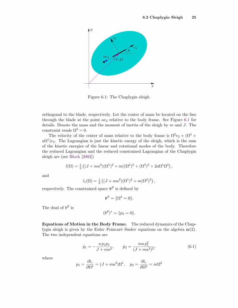
6.2 Chaplygin Sleigh 25
e2
e3
(x, y)
θ
ae2
x
y
Figure 6.1: The Chaplygin sleigh.
orthogonal to the blade, respectively. Let the center of mass be located on the linethrough the blade at the point ae2 relative to the body frame. See Figure 6.1 fordetails. Denote the mass and the moment of inertia of the sleigh by m and J . Theconstraint reads Ω3 = 0.
The velocity of the center of mass relative to the body frame is Ω2e2 + (Ω3 +aΩ1)e3. The Lagrangian is just the kinetic energy of the sleigh, which is the sumof the kinetic energies of the linear and rotational modes of the body. Thereforethe reduced Lagrangian and the reduced constrained Lagrangian of the Chaplyginsleigh are (see Bloch [2003])
l(Ω) = 12
((J +ma2)(Ω1)2 +m((Ω2)2 + (Ω3)2 + 2aΩ1Ω3
),
andlc(Ω) = 1
2
((J +ma2)(Ω1)2 +m(Ω2)2
),
respectively. The constrained space bS is defined by
bS = Ω3 = 0.
The dual of bS is(bS)∗ = p3 = 0.
Equations of Motion in the Body Frame. The reduced dynamics of the Chap-lygin sleigh is given by the Euler–Poincare–Suslov equations on the algebra se(2).The two independent equations are
p1 = − a p1p2
J +ma2, p2 =
map21
(J +ma2)2, (6.1)
wherep1 =
∂lc∂Ω1
= (J +ma2)Ω1, p2 =∂lc∂Ω2
= mΩ2

6.2 Chaplygin Sleigh 26
are the components of nonholonomic momentum relative to the body frame. Ifa 6= 0, equations (6.1) have a family of relative equilibria given by p1 = 0, p2 = const.Linearizing at any of these equilibria, we find that there is one zero eigenvalue andone real eigenvalue. The trajectories of (6.1) are either equilibria situated on theline p1 = 0, or elliptic arcs, as shown in Figure 6.2. Assuming a > 0, the equilibrialocated in the upper half plane are asymptotically stable (filled dots in Figure 6.2)whereas the equilibria in the lower half plane are unstable (empty dots). The ellipticarcs form heteroclinic connections between the pairs of equilibria.
p2
p1
Figure 6.2: The momentum dynamics of the unbalanced Chaplygin sleigh.
If a = 0, momentum dynamics is trivial. Taken together with the analysis ofequations (6.1), this means that we do not observe asymptotic stability if and onlyif a = 0.
The condition a = 0 means that the center of mass is situated at the contactpoint of the sleigh and the plane. The inertia tensor I becomes block-diagonal inthis case, i.e., the direction defined by the constraint is an eigendirection of theinertia tensor.
The Dynamics of the Spatial Momentum. Recall that the spatial angular ve-locity is defined as η = R∗g−1 g = gg−1 ∈ se(2). For the group SE(2) the componentsof η are computed to be
η1 = θ, η2 = x+ yθ, η3 = y − xθ.
The corresponding frame consists of the generators of the left action of SE(2) onitself. The latter are given by the formulae
u1 =∂
∂θ− y
∂
∂x+ x
∂
∂y, u2 =
∂
∂x, u3 =
∂
∂y,
and the corresponding brackets are computed to be
[u1, u2] = −u3, [u1, u3] = u2, [u2, u3] = 0.

6.2 Chaplygin Sleigh 27
The Lagrangian becomes
lR(g, θ) =J +ma2
2(η1)2 +
m
2
((η2 − yη1)2 + (η3 + xη1)2
+ 2aη1[− (η2 − yη1) sin θ + (η3 + xη1) cos θ
]),
and the constraint becomes
−(η2 − yη1) sin θ + (η3 + xη1) cos θ = 0.
The spatial components of the nonholonomic momentum are
µ1 = (J +ma2)η1 −my(η2 − yη1) +mx(η3 + xη1) +maη1(x cos θ + y sin θ),
µ2 = m[(η2 − yη1)− aη1 sin θ
],
µ3 = m[(η2 − yη1) + aη1 cos θ
].
The momentum belongs to the subspace of se∗(2) defined by the equation
−µ2 sin θ + µ3 cos θ − ma
J +ma2(µ1 + yµ2 − xµ3) = 0.
Using (5.7), the dynamics of spatial momentum for the Chaplygin sleigh is
µ1 = λ(x cos θ + y sin θ), µ2 = −λ sin θ, µ3 = λ cos θ,
where λ is is given by the formula
λ =J(µ1 + yµ2 − xµ3)(µ2 cos θ + µ3 sin θ)
(J +ma2)2.
Regardless of the value of a, the spatial momentum of the Chaplygin sleigh is con-served if and only if θ = const, i.e., when the contact point of the sleigh is movingalong a straight line.
Momentum Conservation for the Unbalanced Chaplygin Sleigh. We nowshow that the components of momentum are conserved if one uses the vector fieldsu1, u2, u3 ∈ T SE(2) given by
u1 = cos kθ∂
∂θ+a
ksin kθ
(cos θ
∂
∂x+ sin θ
∂
∂y
), (6.2)
u2 = −ka
sin kθ∂
∂θ+ cos kθ
(cos θ
∂
∂x+ sin θ
∂
∂y
), (6.3)
u3 = − sin θ∂
∂x+ cos θ
∂
∂y, (6.4)
where k2 := ma2/(J +ma2).The structure of the momentum trajectories in Figure 6.2 in combination with
translational symmetry of the sleigh suggests that there may exist vector fields

6.2 Chaplygin Sleigh 28
u = u1(θ)e1 + u2(θ)e2 such that 〈p, u〉 = const. That is, the components of thenonholonomic momentum along a field whose direction and magnitude relative tothe body frame depends on the angle θ may be conserved. Note that θ is not ashape variable as in Theorem 4.4.
Differentiating the quantity 〈p, u(θ)〉 and taking into account equations (6.1)yields
u1 = − map1
(J +ma2)2u2, u2 =
ap1
J +ma2u1.
Using the formula p1 = (J +ma2)Ω1 = (J +ma2)θ, we obtain
du1
dθ= − ma
J +ma2u2,
du2
dθ= au1.
This system defines two independent vector fields (6.2) and (6.3). The field u3 isdefined by formula (6.4) in order to have the sleigh constraint to be written asξ3 = 0, where (ξ1, ξ2, ξ3) are the components of g relative to the frame u1, u2, u3.
Conservation of momentum can be confirmed by the Hamel equations for thesleigh. Computing the Jacobi–Lie brackets for the fields u1, u2, u3, we obtain
[u1, u2] = −k2
acos kθ u1 + k sin kθ u2 + u3,
[u1, u3] = −ka
cos kθ sin kθ u1 − cos2 kθ u2,
[u2, u3] =k2
a2sin2 kθ u1 +
k
acos kθ sin kθ u2,
which implies
C112 = −k
2
acos kθ, C2
12 = k sin kθ, C312 = 1,
C113 = −k
acos kθ sin kθ, C2
13 = − cos2 kθ, C313 = 0,
C123 =
k2
a2sin2 kθ, C2
23 =k
acos kθ sin kθ, C3
23 = 0.
Written relative to the frame u1, u2, u3, the Lagrangian and the constrainedLagrangian become
l(ξ) = 12
((J +ma2)(ξ1)2 +m(ξ2)2 + 2ma cos kθ ξ1ξ3 − 2ma sin kθ ξ2ξ3 +m(ξ3)2
)and
lc(ξ) = 12
((J +ma2)(ξ1)2 +m(ξ2)2
).
The constrained Hamel equations are computed to be
d
dt
∂lc∂ξ1
= 0,d
dt
∂lc∂ξ2
= 0.
Thus, the components of momentum relative to the frame u1, u2, u3 are conserved.

6.3 Chaplygin Sleigh with an Oscillator 29
6.3 Chaplygin Sleigh with an Oscillator
Here we analyze the dynamics of the Chaplygin sleigh coupled to an oscillator. Weshow that the phase flow is integrable, and generic invariant manifolds are two-dimensional tori.
The Lagrangian, Nonholonomic Connection, and Reduced Dynamics.Consider the Chaplygin sleigh with a mass sliding along the direction of the blade.The mass is coupled to the sleigh through a spring. One end of the spring is attachedto the sleigh at the contact point, the other end is attached to the mass. The springforce is zero when the mass is positioned above the contact point. See Figure 6.1where the sliding mass is represented by a black dot and the blade is shown as abold black segment.
The configuration space for this system is R×SE(2). This system has one shape(the distance from the mass to the contact point, r) and three group degrees offreedom.
The reduced Lagrangian l : TR× se(2) → R is given by the formula
l(r, r, ξ) = 12mr
2 +mrξ2
+ 12
((J +mr2)(ξ1)2 + 2mrξ1ξ3 + (M +m)((ξ2)2 + (ξ3)2)
)− 1
2kr2,
where ξ = g−1g ∈ se(2) and k is the spring constant. The constrained reducedLagrangian is
lc(r, r, ξ1, ξ2) = 12mr
2 +mrξ2 + 12
((J +mr2)(ξ1)2 + (M +m)(ξ2)2
)− 1
2kr2.
The constrained reduced energy
12mr
2 +mrξ2 + 12
((J +mr2)(ξ1)2 + (M +m)(ξ2)2
)+ 1
2kr2
is positive-definite, and thus the mass cannot move infinitely far from the sleighthroughout the motion.
The nonholonomic connection is
ξ +Ar,
whereA1 = 0, A2 =
m
M +m, A3 = 0.
The constraint is given by the formula
Ω3 = 0.
The reduced Lagrangian written as a function of (r, r,Ω) becomes
l(r, r,Ω) =12
Mm
M +mr2
+12((J +mr2)(Ω1)2 + 2mrΩ1Ω3 + (M +m)((Ω2)2 + (Ω3)2
)− 1
2kr2.

6.3 Chaplygin Sleigh with an Oscillator 30
The constrained reduced Lagrangian written as a function of (r, r, p) is
lc(r, r, p) =12Mmr2
M +m+
12
(p21
J +mr2+
p22
M +m
)− kr2
2.
The reduced dynamics for the sleigh-mass system is computed to be
Mm
M +mr =
Mmr
(M +m)(J +mr2)2p21 − kr,
p1 = − mr
(M +m)(J +mr2)p1p2 +
m2r
(M +m)(J +mr2)p1r, (6.5)
p2 =mr
(J +mr2)2p21.
We now select a new frame in the Lie algebra se(2) in order to eliminate thesecond term in equation (6.5). Put
e1 = ((J +mr2)−m
2(M+m) , 0, 0), e2 = (0, 1, 0), e3 = (0, 0, 1).
The reduced Lagrangian written in this frame becomes
l(r, r,Ω) =12
Mm
M +mr2 +
12
((J +mr2)
MM+m (Ω1)2 + (M +m)((Ω2)2 + (Ω3)2)
+ 2mr(J +mr2)−M
2(M+m) Ω1Ω3)− 1
2kr2.
Using equations (4.2) and (4.3), the reduced dynamics becomes
Mm
M +mr =
Mmr
(M +m)(J +mr2)M
M+m+1
p21 − kr, (6.6)
p1 = − mr
(M +m)(J +mr2)p1p2, (6.7)
p2 =mr
(J +mr2)M
M+m+1
p21. (6.8)
Relative Equilibria of the Sleigh-Mass System. Assuming that (r, p) =(r0, p0) is a relative equilibrium, equation (6.8) implies r0p0
1 = 0. Thus, eitherr0 = 0 and p0
1 is an arbitrary constant, or, using (6.6), p01 = 0 and r0 = 0. Thus, the
only relative equilibria of the sleigh-mass system are
r = 0, p = p0.
The Discrete Symmetries and Integrability. It is straightforward to see thatequations (6.6)–(6.8) are invariant with respect to the following transformations:
(i) (r, p1, p2) → (r,−p1, p2),
(ii) (r, p1, p2) → (−r, p1,−p2),
6.3 Chaplygin Sleigh with an Oscillator 31
(iii) (t, r, p) → (−t,−r, p),
(iv) (t, r, p1, p2) → (−t, r, p1,−p2).
We now use these transformations to study some of the solutions of (6.6)–(6.8).Consider an initial condition (r, r, p) = (0, r0, p0). Then the r-component of thesolution subject to this initial condition is odd, and the p-component is even. Indeed,let
(r(t), p(t)), t > 0, (6.9)
be the part of this solution for t > 0. Then
(−r(−t), p(−t)), t < 0, (6.10)
is also a solution. This follows from the invariance of equations (6.6)–(6.8) withrespect to transformation (iii). Using the formula
dr(t)dt
∣∣∣t=0
=d(−r(−t))
dt
∣∣∣t=0
,
we conclude that (6.9) and (6.10) satisfy the same initial condition and thus representthe forward in time and the backward in time branches of a the same solution. Thus,r(−t) = −r(t) and p(−t) = p(t).
Next, p1(t) = 0 implies that p2(t) = const and r(t) satisfies the equation
Mm
M +mr = −kr,
and thus equations (6.6)–(6.8) have periodic solutions
r(t) = A cosωt+B sinωt, p1 = 0, p2 = C,
where A, B, and C are arbitrary constants and ω =√k(M +m)/Mm.
Without loss of generality, we set A = 0 and consider periodic solutions
r(t) = r0/ω sinωt, p1 = 0, p2 = p02, (6.11)
which correspond to the initial conditions
r(0) = 0, r(0) = r0, p1(0) = 0, p2(0) = p02.
We now perturb solutions (6.11) by setting
r(0) = 0, r(0) = r0, p1(0) = p01, p2(0) = p0
2. (6.12)
Assuming that p01 is small and using a continuity argument, there exists τ = τp,r0 > 0
such thatr(τp,r0) = 0
for solutions subject to initial conditions (6.12). That is, the r-component is 2τ -periodic if p0
1 is sufficiently small.

6.3 Chaplygin Sleigh with an Oscillator 32
r p1
p2
Figure 6.3: A reduced trajectory of the sleigh-mass system.
Using equation (6.6) and periodicity of r(t), we conclude that p1 is 2τ -periodicas well. Equation (6.7) then implies that p2(t) is also 2τ -periodic. Thus, the reduceddynamics is integrable in an open subset of the reduced phase space. The invari-ant tori are one-dimensional, and the reduced flow is periodic. A generic periodictrajectory in the direct product of the shape and momentum spaces is shown inFigure 6.3.
Using the quasi-periodic reconstruction theorem (see Ashwin and Melbourne[1997] and Field [1980]), we obtain the following theorem:
Theorem 6.1. Generic trajectories of the coupled sleigh-oscillator system in thefull phase space are quasi-periodic motions on two-dimensional invariant tori.
Typical trajectories of the contact point of the sleigh with the plane are shown inFigure 6.4. The symmetry observed in these trajectories follows from the existence,
Figure 6.4: Trajectories of the contact point of the blade for various initial states.
for each group trajectory g(t), of a group element h such that g(t+2τ) ≡ hg(t), where2τ is the period of the corresponding reduced dynamics. It would be interesting tosee if the technique of pattern evocation (see Marsden and Scheurle [1995] andMarsden, Scheurle, and Wendlandt [1996]) extends to the current circumstances.
6.4 Asymptotic Behavior of Momentum Integrals 33
6.4 Asymptotic Behavior of Momentum Integrals
Assuming that the only non-zero term in the right-hand side of the momentumequation (4.7) is 〈p, irτ〉, Theorem 4.4 and Corollary 4.5 give sufficient conditionsfor existence of m independent momentum integrals 〈p, ηa(r)〉, a = 1, . . . ,m. Thefields ηa(r) ∈ bS satisfy equation (4.12), their existence follows from the integrabilityof the distribution associated with the form τ (see Theorem 4.4 for details). In thecoordinate form, equation (4.12) reads
dηb = −Dbaα(r)ηadrα, (6.13)
where the quantities Dbaα(r) are defined by formula (4.11).
The properties of distribution (6.13) resemble the properties of linear homoge-neous systems of differential equations as the coefficients of the differential formsin (6.13) are linear functions in the components of η. It is straightforward to showthat the space of integral manifolds of distribution (6.13) has the structure of anm-dimensional vector space.
Definition 6.2. The Wronskian of the m integral manifolds η = ηa(r), a =1, . . . ,m, is the determinant
W (r) = det
η11(r) . . . η1
m(r)...
...ηm1 (r) . . . ηmm(r)
. (6.14)
The properties of the Wronskian of the system of invariant manifolds of (6.13) aresimilar to those of the Wronskian of the solutions of a system of linear ordinarydifferential equations.
Theorem 6.3. The Wronskian satisfies the equation
d lnW = −Tr τ := −Daaα(r)drα. (6.15)
Proof. Taking into account (6.13) and (6.14), we obtain
∂W
∂rα= −WDa
aα.
Therefore,
dW =∂W
∂rαdrα = −WDa
aαdrα = −W Tr τ,
which is equivalent to formula (6.15).
Corollary 6.4. The Wronskian can be evaluated by the formula
W (r) = W (r0) exp∫ r
r0
Tr τ . (6.16)
The integral in (6.16) is independent of path from r0 to r.Formula (6.16) allows one to obtain the Wronskian explicitly in the multidimen-
tional shape space setting. This result can be used to study the reduced energy levelseven if the momentum integrals cannot be effectively computed. We demonstratethis in the following section for the rolling disk.

6.5 The Rolling Falling Disk 34
6.5 The Rolling Falling Disk
To illustrate the results of §4.3 and §6.4, consider a disk rolling without slidingon a horizontal plane—see Figure 6.5. The configuration space for this systemis (−π/2, π/2) × SO(2) × SE(2). The coordinates on the configuration space aredenoted (θ, ψ, φ, x, y). As the figure indicates, we denote the coordinates of contactof the disk in the xy-plane by (x, y), and let θ, φ, and ψ represent the angle betweenthe plane of the disk and the vertical axis, the “heading angle” of the disk, and“self-rotation” angle of the disk, respectively. Denote the mass, the radius, and the
ϕ
P
Qx
z
y
θ
(x, y)
ψ
Figure 6.5: The geometry for the rolling disk.
moments of inertia of the disk by m, R, A, and B, respectively. The Lagrangian isgiven by the kinetic minus potential energies:
L =m
2
[(ζ1 −R(φ sin θ + ψ))2 + (ζ2)2 sin2 θ + (ζ2 cos θ +Rθ)2
]+
12
[A(θ2 + φ2 cos2 θ) +B(φ sin θ + ψ)2
]−mgR cos θ,
where ζ1 = x cosφ+ y sinφ+Rψ and ζ2 = −x sinφ+ y cosφ, while the constraintsare given by
x = −ψR cosφ, y = −ψR sinφ.
Note that the constraints may also be written as ζ1 = 0, ζ2 = 0.This system is invariant under the action of the group G = SO(2)× SE(2); the
action by the group element (α, β, a, b) ∈ SO(2)× SE(2) is given by
(θ, ψ, φ, x, y) 7→ (θ, ψ + α, φ+ β, x cosβ − y sinβ + a, x sinβ + y cosβ + b).
The fibers of the constraint distribution Dq are spanned by the vector fields ∂θ,∂φ, and −R cosφ∂x −R sinφ∂y + ∂ψ. Therefore,
Sq = Dq ∩ TqOrb(q) = span (∂φ,−R cosφ∂x −R sinφ∂y + ∂ψ) .
6.5 The Rolling Falling Disk 35
We select the basis of the subspace bS ⊂ so(2)× se(2) to be
e1 = (1, 0, R, 0) and e2 = (− tan θ, cos−1 θ,−R tan θ, 0).
The two components of the nonholonomic momentum relative to e1 and e2 are
p1 = Aφ cos2 θ + (mR2 +B)(φ sin θ + ψ) sin θ,
p2 = −Aφ cos2 θ sin θ + (mR2 +B)(φ sin θ + ψ) cos2 θ.
The momentum equations for the falling disk are computed to be
p1 =(
tan θ p1 −B
mR2 +Bp2
)θ, p2 = −mR
2
Ap1θ.
According to Corollary 4.5, there exists a basis η1(θ), η2(θ) of the subspace bS
such that the components 〈p, η1(θ)〉 and 〈p, η2(θ)〉 of nonholonomic momentum areconstants of motion.
We write the momentum levels as c1 and c2, i.e.,
〈p, η1(θ)〉 = c1, 〈p, η2(θ)〉 = c2. (6.17)
Given the momentum levels c1 and c2, equations (6.17) define p1 and p2 as functionsof θ. The vector fields η1(θ) and η2(θ) form the fundamental solution of the linearsystem
dη1
dθ= − tan θ η1 +
mR2
Aη2,
dη2
dθ=
B
mR2 +Bη2. (6.18)
It is possible to write the solutions of system (6.18) in terms of the hypergeometricfunction. See Appel [1900], Chaplygin [1897], and Korteweg [1899] for details. Foradditional work and history of the falling disk see Bloch [2003], Vierkandt [1892]and Cushman, Hermans, and Kemppainen [1996].
Kolesnikov [1985] proves that the disk does not fall, i.e., the absolute value ofthe tilt does not reach the value of π/2 in finite time, for all but a codimension oneset of initial conditions. It is interesting that the proof does not use the explicitformulae for the fields η1(θ) and η2(θ).
Indeed, the boundaries for the tilt of the disk θ are determined by the inequalityUc(θ) ≤ h, where h is the energy level and
Uc(θ) = 12
(p21(θ)/A+ p2
2(θ)/(mR2 +B)
)+mgR cos θ
is the amended potential restricted to the momentum level (6.17). The crucial stepin the proof is to show that limθ→±π/2 Uc(θ) = ∞ for most initial conditions. As in§6.4, consider the Wronskian
W (θ) = det[η1
1(θ) η12(θ)
η21(θ) η2
2(θ)
].
By Liouville’s formula (which is a special case of (6.16))
W (θ) = W (0) exp∫ θ
0− tan θ dθ = W (0)cos θ.
Therefore, W (0) → 0 as θ → ±π/2. Formulae (6.17) thus imply that the absolutevalue of at least one of the momentum components p1(θ), p2(θ) approaches infinityas θ → ±π/2, and so does Uc(θ) for all but a codimension one subset of c = (c1, c2).

7 Conclusions 36
7 Conclusions
In this paper we studied the use of quasivelocities and Hamel equations in thedynamics of nonholonomic systems with symmetry. In particular, we discussed theimportance of the choice of a basis of the tangent bundle of the configuration spacein studying momentum conservation and integrability of nonholonomic systems. Weshowed that these ideas could be very helpful in analyzing specific examples such asthe sleigh-mass system and the falling disk.
In future work we intend to extend some of these ideas to infinite-dimensionalsystems, to the analysis of control of nonholonomic systems, and to the dynamicsof discrete nonholonomic systems, both free and controlled.
8 Acknowledgments
We thank Yakov Berchenko-Kogan, Hernan Cendra, Michael Coleman, Brent Gille-spie, P.S. Krishnaprasad, Jared Maruskin, Richard Murray, Tudor Ratiu, and AndyRuina for numerous discussions, and the referees for helpful suggestions. The re-search of AMB was supported by NSF grants DMS-0604307 and CMS-0408542.The research of JEM was partially supported by AFOSR Contract FA9550-08-1-0173. The research of DVZ was partially supported by NSF grants DMS-0306017and DMS-0604108.
References
Appel, P. [1900], Sur l’integration des equations du mouvement d’un corps pesant derevolution roulant par une arete circulaire sur un plan horizontal; cas particulierdu cerceau. Rendiconti del circolo matematico di Palermo 14, 1–6.
Arnold, V. I., V. V. Kozlov, and A. I. Neishtadt [1988], Dynamical Systems III,Springer-Verlag, Encyclopedia of Math., 3.
Ashwin, P. and I. Melbourne [1997] Noncompact Drift for Relative Equilibria andRelative Periodic Orbits. Nonlinearity 10, 595–616.
Bates, L. and J. Sniatycki [1993], Nonholonomic Reduction, Reports on Math. Phys.32, 99–115.
Bloch, A. M. [2000], Asymptotic Hamiltonian dynamics: the Toda lattice, the threewave interaction and the nonholonomic Chaplygin sleigh, Physica D, 141, 297–315.
Bloch, A.M. [2003], Nonholonomic Mechanics and Control. Interdisciplinary Ap-plied Mathematics, Springer-Verlag.
Bloch, A. M., P. S. Krishnaprasad, J. E. Marsden, and R. Murray [1996], Nonholo-nomic mechanical systems with symmetry, Arch. Rat. Mech. An., 136, 21–99.

REFERENCES 37
Bloch, A.M., P. S. Krishnaprasad, J. E. Marsden, and T. S. Ratiu [1996], The Euler–Poincare equations and double bracket dissipation, Comm. Math. Phys. 175, 1–42.
Carinena, J. F., J.M. Nunes da Costa, and P. S. Santos [2007], Quasicoordinatesfrom the point of view of Lie algebroid structures. J. Phys. A: Math. Theor. 40,10031–10048.
Cendra, H., J. E. Marsden, and T. S. Ratiu [2001a], Lagrangian reduction by stages,Memoirs of the Amer. Math. Soc. 152, Providence, R.I.
Cendra, H., J. E. Marsden, and T. S. Ratiu [2001b], Geometric mechanics, Lagran-gian reduction and nonholonomic systems. In Enquist, B. and W. Schmid, editors,Mathematics Unlimited-2001 and Beyond, pages 221–273. Springer-Verlag, NewYork.
Chaplygin, S.A. [1897], On the Motion of a Heavy Body of Revolution on a Hori-zontal Plane (in Russian). Physics Section of the Imperial Society of Friends ofPhysics, Anthropology and Ethnographics, Moscow 9, 10–16.
Chaplygin, S.A. [1903] On the Rolling of a Sphere on a Horizontal Plane. Mat.Sbornik XXIV, 139–168, (in Russian).
Chaplygin, S. A. [1949], Analysis of the Dynamics of Nonholonomic Systems,Moscow, Classical Natural Sciences; (Russian).
Cushman, R., J. Hermans, and D. Kemppainen [1996], The rolling disc, in NonlinearDynamical Systems and Chaos (Groningen, 1995), Birkhauser, Basel, Boston,MA, Progr. Nonlinear Differential Equations Appl. 19, 21–60.
Euler, L. [1752], Decouverte d’un nouveau principe de Mecanique. Memoires del’academie des sciences de Berlin 6, 185–217.
Field, M.J. [1980], Equivariant dynamical systems, Trans. Am. Math. Soc. 259,185–205.
Greenwood, D.T. [2003], Advanced Dynamics, Cambridge University Press.
Hamel, G. [1904], Die Lagrange–Eulersche Gleichungen der Mechanik, Z. Math.Phys. 50, 1–57.
Jovanovic, B. [1998], Nonholonomic Geodesic Flows on Lie Groups and the Inte-grable Suslov Problem on SO(4). J. Phys. A: Math. Gen. 31, 1415–1422.
Kolesnikov, S.N. [1985], On a Disk Rolling on a Horizontal Plane, Vestn. Mosk. Univ.2, 55–60.
Kolmogorov, A.N. [1953], On dynamical systems with an integral invariant on thetorus (in Russian). Doklady Akad. Nauk SSSR 93, 763–766.

REFERENCES 38
Korteweg, D. [1899], Uber eine ziemlich verbreitete unrichtige Behandlungsweiseeines Problemes der rollenden Bewegung und insbesondere uber kleine rollendeSchwingungen um eine Gleichgewichtslage. Nieuw Archiefvoor Wiskunde 4, 130–155.
Kozlov, V.V. [1985], On the integration theory of the equations in nonholonomicmechanics. Advances in Mechanics 8, 3, 86–107.
Kozlov, V.V. [1988], Invariant measures of the Euler-Poincare equations on Liealgebras. Functional Anal. Appl. 22, 69–70.
Kozlov, V.V. [1995], Symmetries, Topology, and Resonanses in Hamiltonian Me-chanics. Springer-Verlag.
Lagrange, J.L. [1788], Mecanique Analytique. Chez la Veuve Desaint.
Markeev, A.P. [1992]. Dynamics of a Body Being Contiguous to a Rigid Surface. (InRussian), Moscow, Nauka.
Marsden, J.E. and J. Scheurle [1995], Pattern Evocation and Geometric Phasesin Mechanical Systems with Symmetry, Dynamics and Stability of Systems 10,315–338.
Marsden, J.E., J. Scheurle, and J. Wendlandt [1996], Visualization of orbits and pat-tern evocation for the double spherical pendulum, in ICIAM 95: MathematicalResearch, Academie Verlag, (K. Kirchgssner and O. Mahrenholtz and R. Men-nicken, eds.) 87, 213–232.
Marsden, J. E. and T. S. Ratiu [1999], Introduction to Mechanics and Symmetry.Springer-Verlag, Texts in Applied Mathematics, 17; First Edition 1994, SecondEdition, 1999.
Neimark, J. I. and N. A. Fufaev [1972], Dynamics of Nonholonomic Systems. Trans-lations of Mathematical Monographs, AMS, 33.
Poincare, H. [1901], Sur une forme nouvelle des equations de la mecanique. CR Acad.Sci. 132, 369–371.
Rosenberg, R. M. [1977], Analytical Dynamics of Discrete Systems, Plenum Press,NY.
Routh, E.J. [1860] Treatise on the Dynamics of a System of Rigid Bodies. MacMillan,London.
Ruina, A. [1998], Non-holonomic stability aspects of piecewise nonholonomic sys-tems, Reports in Mathematical Physics 42, 91–100.
Veselov, A.P. and L.E. Veselova [1988] Integrable nonholonomic systems on Liegroups. Math. Notes 44, 810–819.

REFERENCES 39
Vierkandt, A. [1892], Uber gleitende und rollende Bewegung, Monatshefte der Math.und Phys., III, 31–54.
Zenkov, D.V. [1995], The geometry of the Routh problem, J. Nonlinear Sci. 5,503–519.
Zenkov, D. V. [2003], Linear Conservation Laws of Nonholonomic Systems withSymmetry. Disc. Cont. Dyn. Syst. (extended volume), 963–972.
Zenkov, D. V. and A. M. Bloch [2003], Invariant measures of nonholonomic flowswith internal degrees of freedom, Nonlinearity 16, 1793–1807.
Zenkov, D. V., A.M. Bloch, and J. E. Marsden [1998], The energy momentummethod for the stability of nonholonomic systems, Dyn. Stab. of Systems 13,123–166.