quaternary science reviews - eidg. forschungsanstalt wsl€¦ · the prehistoric and preindustrial...

lable at ScienceDirect

Quaternary Science Reviews 28 (2009) 3016–3034

Contents lists avai

Quaternary Science Reviews

journal homepage: www.elsevier .com/locate/quascirev

The prehistoric and preindustrial deforestation of Europe

Jed O. Kaplan a,b,*, Kristen M. Krumhardt a, Niklaus Zimmermann b

a ARVE Group, Environmental Engineering Institute, Ecole Polytechnique Federale de Lausanne, Station 2, 1015 Lausanne, Switzerlandb Land Use Dynamics Unit, Swiss Federal Institute WSL, Zurcherstrasse 111, 9031 Birmensdorf, Switzerland

a r t i c l e i n f o

Article history:Received 27 March 2009Received in revised form24 September 2009Accepted 28 September 2009

* Corresponding author. Tel.: þ41 21 693 8058; faxE-mail addresses: [email protected] (J.O. Kaplan

(K.M. Krumhardt), [email protected] (N. Z

0277-3791/$ – see front matter � 2009 Elsevier Ltd.doi:10.1016/j.quascirev.2009.09.028

a b s t r a c t

Humans have transformed Europe’s landscapes since the establishment of the first agricultural societiesin the mid-Holocene. The most important anthropogenic alteration of the natural environment was theclearing of forests to establish cropland and pasture, and the exploitation of forests for fuel wood andconstruction materials. While the archaeological and paleoecological record documents the time historyof anthropogenic deforestation at numerous individual sites, to study the effect that prehistoric andpreindustrial deforestation had on continental-scale carbon and water cycles we require spatially explicitmaps of changing forest cover through time. Previous attempts to map preindustrial anthropogenic landuse and land cover change addressed only the recent past, or relied on simplistic extrapolations ofpresent day land use patterns to past conditions. In this study we created a very high resolution, annuallyresolved time series of anthropogenic deforestation in Europe over the past three millennia by 1) digi-tizing and synthesizing a database of population history for Europe and surrounding areas, 2) developinga model to simulate anthropogenic deforestation based on population density that handles technologicalprogress, and 3) applying the database and model to a gridded dataset of land suitability for agricultureand pasture to simulate spatial and temporal trends in anthropogenic deforestation. Our model resultsprovide reasonable estimations of deforestation in Europe when compared to historical accounts. Wesimulate extensive European deforestation at 1000 BC, implying that past attempts to quantify anthro-pogenic perturbation of the Holocene carbon cycle may have greatly underestimated early human impacton the climate system.

� 2009 Elsevier Ltd. All rights reserved.

1. Introduction

Since the establishment of the first agricultural societies inEurope in the mid-Holocene (Price, 2000), humans have substan-tially altered the European landscape. The most evident andinfluential of these anthropogenic land cover and land use changes(LCLUC) has probably been the clearance of forests and woodlandsfor cropland and pasture and as a source of fuel wood andconstruction materials (Darby, 1956; Hughes and Thirgood, 1982).The rich paleoecological and archaeological record in Europeprovides ample evidence that many European regions experiencedintensive, continuous human occupation throughout the Holocene(e.g., Clark et al., 1989; Brewer et al., 2008; for a review see alsoDearing, 2006). Indeed, some regions of Europe probably experi-enced successive cycles of deforestation, abandonment, andafforestation in the 6000 years of human history preceding theIndustrial Revolution (e.g., Behre, 1988; Bintliff, 1993; Lagerås et al.,

: þ41 21 693 3913.), [email protected]).

All rights reserved.

1995; Berglund, 2000; Vermoere et al., 2000; Cordova and Lehman,2005; Gaillard, 2007). This long history of anthropogenic activityhad important implications for environmental change, fromregional hydrology to possibly global climate, and contains lessonsfor our understanding of what constitutes environmental sustain-ability. In the current study, we attempt to estimate at high spatialand temporal resolution, the patterns of anthropogenic deforesta-tion in Europe from the time agriculture was firmly establishedacross the entire continent until the Industrial Revolution.

Though it is certain that the forests of many European countrieswere substantially cleared before the Industrial Revolution (inEurope, ca. 1790–1900), we lack a clear dataset describing theprogression of deforestation that occurred during prehistoric andpreindustrial times. The first studies that attempted to map thetemporal pattern of anthropogenic land use and land cover changeat the global to continental-scale before AD 1850 were limited intemporal extent to AD 1700 and relied on simplistic relationshipsbetween 20th century patterns of land use to extrapolate to earliertimes (Ramankutty and Foley, 1999; Klein Goldewijk, 2001).constructed a contemporary permanent croplands map asa starting point for their model, and then ran a land cover changemodel backwards in time to the year 1700 using any available

mailto:[email protected]



www.sciencedirect.com/science/journal/02773791

http://www.elsevier.com/locate/quascirev

J.O. Kaplan et al. / Quaternary Science Reviews 28 (2009) 3016–3034 3017

historical cropland data as a constraint. This simple model used analgorithm for distributing cropland spatially over time, leavingcountry boundaries and other relics in the database.

The HYDE database of global historical land use change (KleinGoldewijk, 2001) was developed using population estimates asa proxy for the extent of agriculture over the past 300 years,including both cropland and pastureland. The starting point of thismodel was a spatially explicit global population map overlaid withcountry boundaries. Historical population records for each countrywere then used for temporal variation, while, using the assumptionthat high population density areas stay in the same place over time,spatial variation was provided by population distribution. Next,modern estimates of total cropland and pastureland per countrywere allocated back in time according to population density, withareas of higher population density being the first to be converted tocropland and pasture.

Most recently, Pongratz et al. (2008) synthesized a dataset ofglobal LCLUC for the historical period (AD 800 – Present) thatincludes crop, pasture and natural land cover fractions. In this study,the authors referenced published maps of agricultural areas fromthe two studies described above (Ramankutty and Foley,1999; KleinGoldewijk, 2001) as a starting point, then found the ratio of total landarea used per capita for crop and pasture at AD 1700 for each country,and finally, using this ratio, scaled estimates of crop and pasture areaby historical population estimates per country. This method is basedon two major assumptions: 1) per capita land use for crop andpasture did not change prior to AD 1700, (though ranges provided inthis dataset explicitly include uncertainties in estimates of pastpopulation and technological change), and 2) the spatial pattern ofcrop and pasture areas was exactly the same throughout thehistorical period as it was at AD 1700, i.e., the amount of land undercultivation in each gridcell at any given time is simply the AD 1700value scaled by relative population change. In this way, the Pongratzet al. (2008) method propagates all uncertainties associated with theyear AD 1700 land use maps in the Ramankutty and Foley (1999) andHYDE datasets (Klein Goldewijk, 2001).

In a global study assessing the effects of anthropogenic LCLUCsince the mid-Holocene, Olofsson and Hickler (2007) also relied onthe HYDE dataset of land cover change from AD 1700 onward. Forfour time slices prior to AD 1700, the authors used simple maps andliterature on the spread of human civilization with historical worldpopulation records to estimate the extent of permanent and non-permanent agriculture since the mid-Holocene. As these referencesdo not explicitly deal with land cover, all lands classified as beingunder ‘‘states and empires’’ were simply assumed to be 90% underagriculture, and a lower fraction of anthropogenic land use wasassigned to areas occupied by ‘‘agricultural groups’’. The crudespatial and temporal resolution of this approach makes it unsuit-able for anything more detailed than a global-scale assessment ofhuman impact on the terrestrial biosphere on millennial time-scales. None of the currently available LCLUC datasets incorporateobservations of land cover change from the historical record beforeAD 1700, or from paleoecological or archaeological data synthesis.Our new approach uses historical observations of land cover overthe last two millennia to model the changing relationship betweenpopulation and forest cover and overcome some of the limitationsof previous datasets of prehistoric and preindustrial LCLUC.

It is likely that human modification of the environment,particularly through deforestation, would have had consequencesfor local to regional scale hydrology and climate, through changesin albedo, surface roughness and the balance of transpiration torunoff and groundwater recharge. A number of studies havedemonstrated the sensitivity of regional climate to realistic levels ofhuman impact (Eugster et al., 2000; Dumenil Gates and Ließ, 2001).In contrast, the effects of prehistoric and preindustrial

anthropogenic LCLUC on global climate are currently the subject ofa lively debate (Ruddiman, 2007). Using a top down approach,a number of studies (Ruddiman et al., 2004; Vavrus et al., 2008)demonstrated the sensitivity of global climate to Holocene trendsin atmospheric CO2 and methane concentrations. As Ruddiman hasargued (Ruddiman, 2005), these greenhouse gases could have hadanthropogenic origins from deforestation resulting in CO2 emis-sions, and the introduction of substantial populations of ruminantanimals and development of rice agriculture, which increasedmethane emissions to the atmosphere. On the other hand, bottomup modeling studies that attempted to estimate prehistoric andpreindustrial anthropogenic CO2 emissions concluded that theseemissions would have been too small to have had a substantialeffect on global climate (DeFries et al., 1999; Olofsson and Hickler,2007; Pongratz et al., 2009), and rather attribute the observedtrends in CO2 and methane concentrations to natural sources.However, given the limitations of these datasets described above, itis conceptually possible that they significantly underestimateanthropogenic emissions. Recently, a paleoecological datasynthesis by Nevle and Bird (2008) concluded that afforestationafter the collapse of populations in Latin America following Euro-pean contact could have been significant enough to perturb theglobal carbon cycle and climate system.

In light of these confounding results and the limitations ofcurrent datasets, we attempt a new analysis of preindustrial andprehistoric anthropogenic LCLUC using updated datasets ofhistorical population trends, climate and soils, and a novel methodfor inferring the relationship between population and land usebased on observational forest cover data. Our goal is to quantifyuncertainties in both population size and the rate of technologicalchange and to estimate the sensitivity of our model to these drivingvariables. Our study focuses on Europe and neighboring regionsbecause 1) this area has a record of human impact that covers theentire Holocene, 2) detailed estimates of historical population areavailable at national and sub-national level, and 3) the richarchaeological and paleoecological records enable us to makea least a qualitative evaluation of our model results.

2. Materials and methods

To estimate the deforestation of Europe, we developed a modelof prehistoric and preindustrial LCLUC. The model is driven byhuman population size and constrained by suitability maps foragriculture and pasture, which are in turn based on griddeddatasets of climate and soil properties. A relationship betweenpopulation density and cleared area determines the amount of landthat will be deforested by the human population at any given time.The suitability maps ensure that the most productive crop andpasturelands will be deforested first, with deforestation spreadingto increasingly marginal land as population densities increase.A schematic of the deforestation model is presented in Fig. 1.Development and application of the deforestation model involvedfour steps: 1) assembling a spatially explicit database of humanpopulation from 1000 BC to AD 1850, 2) developing a relationshipbetween population density and amount of cleared land,3) preparing gridded maps of relative land suitability for crop andpasture and 4) combining these to create maps of forest cover.

2.1. Spatial and temporal domain

The spatial domain for our analysis is the area defined by thereference map projection and grid recommended by the EUINSPIRE Directive (Annoni et al., 2001; Annoni, 2005). This domainroughly covers Europe and neighboring areas from Iceland andPortugal to the Urals and from the Mediterranean to northernmost

Model of land suitability to cultivation and pasture

Population estimates foreach population region (1000 BC – AD 1850)

Forest cover – population relationship

Historical forest cover estimates for each region

(1000 BC – AD 1850)

Historical forest cover maps for region (1000 BC – AD 1850)

High quality agricultural landis cleared first, marginal land

is cleared next.

Climate data Soils data

Datasets of land suitabilityfor cultivation and pasture

Fig. 1. Schematic of the preindustrial anthropogenic deforestation model, depictingthe steps taken for spatial variability (left-hand side) and temporal variability (right-hand side) in order to generate historical land clearance maps of Europe.

J.O. Kaplan et al. / Quaternary Science Reviews 28 (2009) 3016–30343018

Fennoscandia, covering part or all of more than 40 countries inEurope, North Africa and the Near East (Fig. 2). The temporaldomain of our study covers the period 1000 BC to AD 1850. By1000 BC, permanent agriculture was well-established everywherein our spatial domain (Ammerman and Cavalli-Sforza, 1971; Price,2000; Pinhasi et al., 2005), except for Iceland and the FaeroeIslands, and thus provides a reasonable starting point for ouranalysis that will not be complicated by the need to simulate thedispersal and establishment patterns of agricultural societies.

2.2. Historical population data

We developed a database of annually resolved populationestimates from 1000 BC to AD 1850 for 52 regions of Europe, NorthAfrica and the Near East (Fig. 2). Generally, one population regionrepresents one country with the national boundaries of 1975,though in some cases, population regions are an amalgamation ofcountries, and in other cases, nations are divided into sub-regions.The population database is mainly based on the charts and spotestimates in McEvedy and Jones (1978), supplemented by otherinformation where possible.

McEvedy and Jones (1978) contains continuous curves of totalpopulation for the period 400 BC to AD 1975 for a number ofpopulation regions covering the entire world. Curves for populationregions in our study area were scanned and then rectified anddigitized using GraphClick software (Arizona Software). To producepopulation estimates for the period prior to 400 BC, we extractedspot estimates for specific years from the text of McEvedy and Jones(1978), added these point estimates to the digitized data, and thenlinearly interpolated the data to produce estimates of annualpopulation from 1000 BC to AD 1850.

Because McEvedy and Jones (1978) treat the whole of Russia-in-Europe as a single population region, we attempted to distributethe Russian population across this very large area by using

additional data sources. Lewis and Leasure (1966) provideestimates of the population of 12 major economic regions inEuropean Russia for AD 1851. We distributed the total population ofEuropean Russia in AD 1850 from our McEvedy and Jones-baseddataset according to the Lewis and Leasure (1966) estimate andscaled every prior year by the spatial distribution at AD 1850. Whilethis simplification ignores, e.g., urban migration before AD 1851, wefeel that the result is better than arbitrarily spreading the totalpopulation of European Russia over the entire area of the country,which would result in an unrealistic concentration of population inthe southern, most agriculturally suitable part of European Russia(Chernozem belt). Similarly, to create population estimates for EastPrussia, we obtained time slice estimates of population forseveral times in the past millennium (Jurkat, 2004), and reducedpopulations for Poland and the Russia West region accordingly.

The population estimates provided by McEvedy and Jones(1978), the main source of primary information for our database,have acknowledged uncertainties that increase with time into thepast. To address these uncertainties and provide a model sensitivitytest, we produced a range of alternative historical populationestimates. Clark (1977) and Biraben (1979), provide estimates ofpopulation for Europe and the parts of North Africa and the NearEast that are included in our spatial domain at selected time slicesover the last three millennia. With these alternative estimates, wescaled the population within each region of our spatial domain tocreate continuous upper- and lower-bound estimates of populationfor the period 1000 BC to AD 1850.

In general, for earlier periods, McEvedy and Jones (1978)contained the most conservative, i.e., lower, population estimates,while in later periods they tended to be at the upper bound ofestimations as compared to the other two references. The upper-and lower-bound time slice estimates of population for Europe andsurrounding areas (our spatial domain) were linearly interpolatedto create an annual time series, and then divided by the sumof estimates for all 52 population regions from McEvedy andJones (1978) to produce a ratio for both the upper and lowerboundaries. Subsequently, for each year and for each populationregion, upper- and lower-bound ratios were multiplied by theoriginal population estimates from McEvedy and Jones (1978), toobtain annual upper- and lower-bound population estimates foreach population region.

2.3. The relationship between population density and forest cover

In preindustrial societies, human population is the major driverof anthropogenic LCLUC (Darby, 1956; Mather et al., 1998b; Matherand Needle, 2000). As population density increases in a given area,the amount of land required to support this population willincrease. Mather et al. (1998b) outlined two theoretical reasons forexpecting a positive relationship between population and defor-estation for preindustrial times. First, population growth stimulatesthe expansion of arable land for growing more food, which, in areasthat would naturally be forested, generally results in deforestation.Secondly, a growing population means increased usage of forestproducts such as wood for fuel and construction materials, whichcan lead to an overall decline of forest area.

Population pressure on a landscape may be ameliorated bymigration, trade and use of non-agricultural food resources (e.g.,fishing), which may increase populations through external factorsand by in situ improvements in the efficiency of the land basethrough technological innovation, development, and specialization.At a certain level of technological development, generally coin-ciding with industrialization and urbanization, most countriesexperience a ‘‘forest transition’’ where the relationship betweenpopulation and the area of land under cultivation becomes

Fig. 2. Numbered map showing the population regions of our preindustrial anthropogenic deforestation model corresponding to the numbers listed for each region in Table 3.Regions with similar deforestation trends (see Fig. 8) throughout our study period are grouped using a certain color, while areas in gray ere not considered in this study.


uncoupled and in many cases even reverses, with afforestationconcurrent with population growth (Mather, 1992, 2004; Rudelet al., 2005). Because the aim of this project is to develop a timeseries of deforestation prior to industrialization and thereforebefore forest transitions took place, and given that climate vari-ability in Europe over the last 3000 years has been relatively small(Davis et al., 2003; Wanner et al., 2008), we assume that populationchange is the primary driver of changes in forest area for the years1000 BC to 1850.

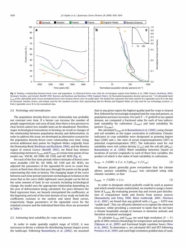
Mather (1999) proposes a sigmoidal log-linear relationshipbetween population density and forest cover during the timepreceding the forest transition, based on historical population andforest cover data from France. We expand on this approach by usingdata from other countries and building a relationship betweenpopulation and forest cover to drive our model. Historical forestcover data was available for four European countries (Fig. 3a):Denmark, Ireland, France, and Sweden (Mather, 1999; Bradshaw,2004). Among these historical forest cover data, the France data(Mather, 1999) is the most detailed and reliable because it is basedon a wide variety of sources (e.g., historical records, statisticalsources), but the other data is also valuable since it captures overallforest cover trends for diverse regions of Europe, necessary forbuilding our generalized relationship. Since there are differences inthe proportion of arable land and land productivity among coun-tries, we needed to normalize both our population density andforest cover records to develop a population density-forest coverrelationship that focuses on the key drivers in the relationship andeliminates country-specific biases.

2.3.1. Normalizing the population density axisHistoric agrarian societies tended to exist only where people

could grow food, and therefore a better approximation of

population density within a region is population density on thecultivatable land area (Acrop) within the population region (Pdens).Next, we needed to account for the quality of the usable land withina region. This was done by dividing the Pdens by the land suitabilityfor cultivation on the usable land (Smean), thus creating normalizedpopulation density (Pnorm) (Table 2).

2.3.2. Normalizing the forest cover axisIn order to fit an inverse relationship between forest cover and

population for preindustrial times, data for the years after the foresttransition, where forest cover starts increasing with time (Fig. 3a),were eliminated from the forest cover datasets. Furthermore,because people typically cleared land to grow crops, createpastures, or use forest products, the forest cover estimates for eachcountry were normalized by subtracting the unusable land (i.e.,land that can not be used for crops, pasture, or that is generallyuninhabitable by humans) from the potential maximum forestcover for each country. Therefore, the normalized dependentvariable became forest cover only on usable land (FCnorm).

With both axes normalized, the time series of populationdensity and forest cover for these four countries show a consistentrelationship (Fig. 3b). Following Mather (1999), we build a ‘‘standardscenario’’ by fitting a sigmoidal curve to the FCnorm versus Pnorm

relationship using nonlinear least squares regression (R Develop-ment Core Team, 2005). The equation takes the form,

FCnorm ¼0:9958

1þ ebðc�PnormÞ(1)

where b and c are shape parameters that represent technologicaldevelopment and intensification.

0

10

20

30

40

50

60

70

80

90

100%( revoc tseroF

)

1000 1200 1400 1600 1800Time (years AD)

a

0.0

0.1

0.2

0.3

0.4

0.5

oitcarf revoc tserof dezilamro

Nn

1 10 100 1000Normalized population density (persons km−2)

b

0.00.20.40.60.81.0

1 10 100

c

Denmark Sweden Ireland France England−Wales Boeotia (Greece)

Fig. 3. Finding a relationship between forest cover and population. (a) Historical forest cover data for six European regions from Mather et al. (1999; France), Bradshaw (2004;Denmark, Sweden, and Ireland), Bintliff (1993; Boeotia) and Rackham and Rackham (1994; England–Wales). (b) Normalized population density (persons km�2 of cultivatable land/Scrop of the cultivatable land) versus normalized forest cover fraction (forest cover on usable land). The dashed line represents the lower portion of a sigmoidal curve fit to the datafor Denmark, Sweden, France, and Ireland, used for the standard scenario. Dots representing data for Boeotia and England–Wales are only used for our technology scenario. (c)Entire sigmoidal curve fit to the normalized data.


2.4. Technology and intensification

The population density-forest cover relationship was probablynot constant over time. If a farmer can increase the number ofpeople supported per unit area of land, then there is less pressure toclear forests and/or less suitable land can be abandoned. Therefore,major technological innovations in farming can result in changes ofthe relationship between population density and deforestation. Inorder to address this issue, we developed an alternative scenario forthe population density-forest cover relationship over time. Usingseveral additional data points for England–Wales originally fromthe Domesday Book (Rackham and Rackham,1994), and the Boeotiaregion of central Greece (Bintliff, 1993), we fitted four distinctrelationships between Pnorm and FCnorm at certain time points of ourmodel run: 350 BC, AD 1000, AD 1350, and AD 1830 (Fig. 4).

For each of the four time periods where estimates of forest coverwere available (350 BC, AD 1000, AD 1350 and AD 1830), weadjusted the parameters of the sigmoidal fit curve to create fourcurves at fixed time slices that pass through the points on the graphrepresenting this time in history. The changing shape of the curvebetween each time period represents technological evolution in thesense that as the curve shifts rightward, more people can be fed onthe same amount of land. In our scenario including technologicalchange, the model uses the appropriate relationship depending onthe year of deforestation being calculated. For years between thefixed regression lines, we linearly interpolated the coefficients; atthe beginning and end of the time domain of our study we held thecoefficients constant to the earliest and latest fixed curves,respectively. Shape parameters of the sigmoidal curve for thestandard scenario and the individual fixed time slices are presentedin Table 1.

2.5. Estimating land suitability for crops and pasture

In order to make spatially explicit maps of LCLUC, it wasnecessary to devise a scheme for distributing human impact acrossthe landscape. Following Ramankutty et al. (2002), we assumed

that in any given region the highest quality land for crops is clearedfirst, followed by increasingly marginal land for crop and pasture, aspopulation pressure increases. For each 50 � 50 gridcell in our spatialdomain, we computed a fractional value for each of two indices:land suitability for cultivation (Scrops) and land suitability forpasture (Susable).

We calculated Scrops as in Ramankutty et al. (2002), using climateand soil variables as the major constraints to cultivation. Climaticindicators to crop suitability were designated as growing degreedays (GDD) and a, the ratio of actual evapotranspiration (AET) topotential evapotranspiration (PET). The indicators used for soilsuitability were soil carbon density (Csoil) and the soil pH (pHsoil).Ramankutty et al. (2002) fitted suitability functions (based onlocations of current croplands) to each of these four variables, theproduct of which is the index of land suitability to cultivation,

Scrops [ f ðGDDÞ 3 f ðaÞ 3 f ðpHsoilÞ 3 f ðCsoilÞ (2)

Because plants generally grow everywhere that the climateallows, pasture suitability (Susable) was calculated using onlyclimatic variables, so that

Susable [ f ðGDDÞ 3 f ðaÞ (3)

In order to designate which gridcells could be used as pastureand which would remain undisturbed, we needed to assign a lowerlimit of Susable. By evaluating present day and recent past distribu-tion of crop/pasture lands and forests from various sources(Ramankutty and Foley, 1999; Klein Goldewijk, 2001; Paivinenet al., 2001), we found that any gridcell with a Susable > 0.075 was‘‘usable land’’. This cut-off point allowed us to explain the observedclearance, while providing a constraint to lands that do not havea climate hospitable enough to humans or domestic animals andtherefore remained unchanged.

To calculate Scrops and Susable we used high resolution (50 � 50)grids of 20th century climatology for temperature and precipitation(Hijmans et al., 2005) and fractional bright sunshine hours (Newet al., 2002). To determine a, we calculated AET and PET followingPrentice et al. (1993) and used high resolution gridded data of sand,

Table 2Abbreviations used for describing the preindustrial anthropogenic deforestationmodel.

Variable Definition Unit

Variables used to calculate Scrops and Susable

GDD Growing degree days, an annual sum of dailymean temperatures over 5 �C

day �C

AET Actual evapotranspiration, minimum of theevaporative demand and supply

mm h�1

PET Potential evapotranspiration, evaporativedemand

mm h�1

a Moisture index; AET/PET fractionCsoil Soil carbon density kg C m�2

pHsoil Soil pH pH scale

Input variablesScrops Gridded dataset of land suitability for

cultivation indexfraction

0.0

0.1

0.2

0.3

0.4

0.5

0.6

0.7

0.8

0.9

1.0

oitca

rf re

voc t

sero

f de

zila

mro

Nn

1 10 100 1000

Normalized population density (persons km−2)

CB

053

0001

D

A

0531

D

A

0381

D

A

Fig. 4. Addressing technological progress in the relationship between populationdensity and forest cover. Lines were fit to certain points in time for the data available.The line for year 350 BC is fit to two points: Boeotia at 400 BC (Bintliff, 1993) and theearliest data point for England–Wales at 300 BC (Rackham and Rackham, 1994). The AD1000 line is fit to three points: the start points for the forest cover data for France andIreland (AD 934 and AD 1003, respectively) (Mather 1999; Bradshaw, 2004), and theDomesday estimate for England–Wales at AD 1083 (Rackham and Rackham, 1994). Theline for AD 1350, representing the Black Death event, is fitted for a forest cover esti-mate in England–Wales at the time of the Black Death (Rackham and Rackham, 1994)and the point on the France line where the distinct population drop due to the BlackDeath occurs (Mather 1999). Finally, the AD 1830 line is fitted to the last time pointbefore the forest transition in France (Mather 1999) and Sweden (Bradshaw, 2004),and the last point of the Irish data (no forest transition occurred within the data)(Bradshaw, 2004). The arrows indicate the movement of the relationship with time.The dashed line is the population-forest cover relationship used in the standardscenario. Refer to Fig. 3 for color key.


clay, and organic matter content from the Harmonized World SoilDatabase (FAO/IIASA/ISRIC/ISSCAS/JRC, 2008) to calculate availablesoil water content following Saxon and Rawls (2006). The Harmo-nized World Soil Database also supplied data on Csoil and pHsoil forthe top 30 cm of soil, the soil indicators used in the function tocalculate Scrops.

Susable Gridded dataset of land suitability forpasture index

fraction

P Total population of a population region(annually, from 1000 BC to 1850)

persons

Agridcell Area of a gridcell (varies with latitude) km2

Constants for each population regionAcrops Area suitable for growing crops; Agridcell � Scrops km2

Ausable Area that is suitable for pasture, i.e. usable;sum of Agridcell with a Susable > 0.075

km2

Smean Mean Scrop of usable land (where Susable > 0.075) fractionCfrac Fraction of the usable land suitable to grow crops fraction

Variables for each population regionPdens Population density on Acrops persons km�2

�2

2.6. Simulating anthropogenic deforestation

Using the datasets and model described above, we simulatedannually resolved anthropogenic deforestation at 50 resolution forthe period 1000 BC to AD 1850 (Fig. 1). The modeling procedure hadfive parts (refer to Table 2 for variable definitions):

1. From the land suitability data, the summary statistics Acrops,Ausable, Smean, and Cfrac are calculated for each populationregion.

Table 1Values of shape parameters, b and c, for various curve fits of Pnorm vs. FCnorm

described by Eqn. (1), which vary in accordance to technological progress.

Curve b c

Standard scenario �3.0 1.40350 BC �5.0 0.911000 AD �6.0 1.361350 �7.5 1.691830 �7.0 1.85

2. Year and population estimates are read in, calculating Pdens andPnorm for each population region at each time slice. FCnorm isthen calculated according to Eq. (1).

3. DFfrac, the current cleared fraction of usable land, is calculatedby subtracting FCnorm from one. If DFfrac becomes greater thanor equal to Cfrac with time, then the fraction of the gridcell usedfor growing crops is one and the remaining portion of DFfrac

would then be designated as pasture, Fusable. Fcrops cannot belarger than Cfrac. However, if DFfrac is less than Cfrac, then Fcrops issimply the ratio of DFfrac to Cfrac. This ratio will approach 1 asdeforestation continues; i.e., if the cleared fraction of usableland is less than the amount of high quality cultivatable land,then the cleared fraction, DFfrac, will be 100% cropland and 0%pasture. As population density increases with time, DFfrac canbecome larger than Cfrac, and lands of inferior quality arecleared for pasture.

4. The gridded variables, Gcrops and Gusable, are computed for eachtime step. Within each gridcell of Europe, Gcrops is calculated bymultiplying the value of Fcrop by the gridcell’s crop suitability,Scrops, used here as the fractional value of the gridcell suitable forgrowing crops. Gusable, however, is calculated by multiplyingFusable by the difference of Scrops and Susable. We must use thedifference between Scrops and Susable because here these twoindices are used as fractional values, and Susable will alwaysinclude the fraction of land deemed as high quality cropland, Cfrac.

5. The total anthropogenic land use of each gridcell, GtotalLU iscalculated by simply taking the sum of Gcrops and Gusable.

Pnorm Normalized population density, Pdens/Scrops persons kmFCnorm Forest cover fraction of usable land fractionDFfrac Cleared fraction of usable land, 1 � FCnorm fractionFcrops Fraction of cleared land used for crops fractionFusable Fraction of cleared land used for pasture (usable) fraction

Gridded variables (model output)Gcrops Fraction of gridcell that is cropland; Fcrops � Scrops fractionGusable Fraction of gridcell that is pasture;

Fusable � (Susable � Scrops)fraction

GtotalLU Total land use (cleared) fraction of gridcell;Gcrops þ Gusable

fraction


3. Results

3.1. Land suitability for crops and pasture

Our simulation of land suitability for crops and pasture (Fig. 5)reveals that Scrops is markedly heterogeneous over the Europeanlandscape. This model, based on climate variables (GDD and a) andsoil variables (pHsoil and Csoil), shows the richest cultivation area tobe the central band through the mid-latitudes of Europe (Fig. 5a).This central band is even more evident on the map of landsuitability to pasture (Susable), which was produced by a modelconstrained only by the climate variables GDD and a (Fig. 5b).Northern latitudes (the Nordic countries and northern Russianregions) of both maps are constrained by low temperatures, whilesouthern latitudes (North African regions) are constrained by lackof water.

Land appears to be especially suited for cultivation in theregions bordering the Mediterranean Sea (excluding the desertcoasts of Libya) and in the black earth region of the eastern Euro-pean steppes. Soil characteristics put a constraint on Scrops in areassuch as southwestern France and mid-southern Sweden. Centraland southern Russian regions display consistently rich farmland,while central European soils are variable and broken up bymountain ranges such as the Alps, Pyrenees, and Carpathians.These high altitude regions are restrained by climate limitationsand are thus deemed unusable by this model. Overall, the region ofEurope, although variable in soil quality and topography, is rich incultivatable land area and is suitable for pasture in most mid-lati-tude areas.

3.2. Historical forest cover estimates for the standard scenario

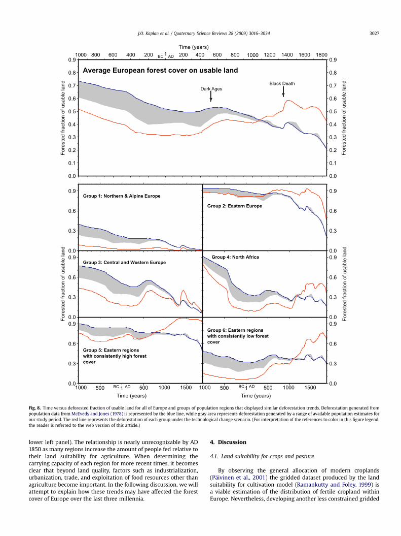
Historical forest cover estimates are presented in Fig. 8 andTable 3 as forested fractions of the usable land in each populationregion. Fig. 8 presents the time history of average forest cover in allof Europe and within six super-regions of Europe that showedsimilar trends in forest cover. Our standard scenario is presented in

Fig. 5. Maps of land suitability for cultivation (a) and pasture (b). Land suitability to cultivincluded both soil characteristics (soil pH, soil carbon density) from Harmonized Worldprecipitation, and potential sunshine hours) from New et al. (2002) and Hijmans et al. (20

blue and includes an area of error due to uncertainty in populationestimations; the technology scenario is presented in red.

At the earliest time slice of our model, 1000 BC (Fig. 6, top leftpanel), the Near Eastern regions (Iraq, Syria-Lebanon, andPalestine-Jordan) clearly display widespread deforestation due toboth the high population densities already achieved by that timeand the low proportion of high quality agricultural land. Severalsmall parts of central Europe (within Belgium, Switzerland, andAustria) display 70% clearance by 1000 BC, but overall the bulk ofthe European continent retains its forest cover in areas that werestill mainly occupied by prehistoric societies. For example, NorthAfrican and Eastern European regions display little or no defores-tation at this time slice. In contrast, regions with very smallamounts of cultivatable land such as Norway and Sweden hadalready cleared much of their usable land (a small area compared tothe total area of the region) to be able to support their populationsat this time (Table 3, Fig. 8).

Seven hundred years later, by 300 BC (Fig. 6, top right panel),forest clearance (agricultural areas) increased significantly in someparts of Europe and surrounding areas. The areas suited to agri-culture within Greece, Algeria, and Tunisia, in particular, wereclassified as up to 90% under agriculture, while central and westernEuropean regions are calculated to have been between 10% and 60%deforested. Regions of the Near East continued to maintain theirhigh population densities, while Eastern Europe, with lowpopulation densities, remained highly forested.

By AD 350 (Fig. 6, middle right panel), the collapse of theclassical empires in Greece and neighboring regions led to lowerpopulation densities and afforestation in these areas relative to 300BC. Central European regions, such as France, Germany, and Poland,showed moderately increased forest clearance (up to 90% in someareas) and Russian regions were just beginning to display signifi-cant levels of deforestation at this time. Although some regionsexhibited a slight decrease in deforested area between AD 350 andAD 1000 (e.g., Central and Western Europe, see Fig. 8, group 3), netclearance of woodland in Europe did not change significantly(Fig. 6, middle panels). However, some regions that were previously

ation (Scrops) was simulated as in Ramankutty et al. (2002). Constraints to cultivationSoil Database (FAO/IIASA/ISRIC/ISSCAS/JRC, 2008) and climate data (air temperature,05). Land suitability to pasture (Susable) was constrained solely by the climate data.

Table 3Numbered list of population regions corresponding to the map in Fig. 2 with estimates of percent usable land (land available for clearing for agriculture), and percent of forestcover on usable land by years 1000 BC, 500 BC, AD 1, AD 500, AD 1000, AD 1350, AD 1400, and AD 1850 for each region.

% Forest cover on usable land:

Region % Usable land 1000 BC 500 BC AD 1 AD 500 AD 1000 AD 1350 AD 1400 AD 1850(Black Death)

Northern & Alpine Europe1 Denmark 29.2 32.3 29.7 25.6 17.6 12.8 8.4 15.0 3.12 Norway 95.5 1.9 1.6 1.3 1.0 0.6 0.3 0.6 0.03 Sweden 79.8 27.1 24.2 17.7 13.8 9.9 4.8 8.8 0.74 Finland 86.7 67.8 65.1 17.0 8.5 5.4 4.2 3.0 0.05 Iceland 99.6 100.0 100.0 100.0 100.0 0.0 0.0 0.0 0.06 Belgium–Luxembourg 9.2 30.4 34.4 27.1 30.2 26.6 7.1 11.6 1.27 Austria 50.0 49.3 45.5 23.8 27.8 19.4 6.7 8.2 2.18 Netherlands 9.3 64.1 34.2 21.3 20.1 13.0 4.9 7.5 0.99 Scotland 72.9 12.5 6.8 7.2 4.8 2.8 0.7 1.3 0.110 Switzerland 58.1 41.8 20.8 18.0 18.9 17.6 5.0 9.1 1.311 Russia: Northwest 87.8 70.4 66.6 49.4 38.0 30.4 9.3 11.9 1.1

Group 1 average 48.0 45.2 39.0 28.0 25.5 12.6 4.7 7.0 1.0

Eastern Europe12 Belarus 16.8 94.6 93.6 88.1 82.5 77.1 44.2 51.1 8.013 Russia: C. Chernozem 6.4 98.1 97.8 96.0 94.0 91.9 73.2 78.3 23.214 Russia: Central 32.1 92.2 90.8 83.1 75.7 69.1 34.3 40.8 5.415 Ukraine: East 1.7 98.9 98.8 98.0 97.0 96.0 85.9 88.9 40.616 Moldova 0.8 98.7 98.5 97.4 96.1 94.8 81.8 85.6 33.417 Ukraine: South 0.6 99.1 99.0 98.4 97.7 96.9 89.0 91.4 47.818 Ukraine: West 8.9 96.5 95.9 92.4 88.6 84.9 57.0 63.7 12.719 Russia: Ural 70.9 98.6 98.4 97.2 95.9 94.5 80.8 84.7 31.920 Russia: Volga 3.7 99.1 99.0 98.3 97.6 96.8 88.6 91.0 46.621 Russia: Volgo Viatsk 36.3 95.2 94.4 89.4 84.3 79.5 47.6 54.6 9.122 Baltics 35.1 93.0 91.8 84.8 77.9 71.7 37.2 43.9 6.123 Bulgaria 7.1 92.0 93.6 80.7 71.0 70.5 68.0 76.7 28.924 East Prussia 14.0 95.0 93.2 84.6 79.2 66.1 35.7 40.6 6.525 Hungary 0.6 85.9 84.3 85.3 89.8 73.2 42.2 52.3 14.326 Romania 11.5 83.1 82.6 82.1 87.1 83.4 62.2 70.9 17.527 Yugoslavia 9.4 85.0 75.2 61.2 56.9 55.6 41.1 54.4 19.4

Group 2 average 16.0 94.1 92.9 88.6 85.7 81.4 60.5 66.8 22.0

Central & Western Europe28 Czechoslovakia 23.0 76.0 65.2 37.5 43.6 31.3 12.7 16.3 3.229 France 7.4 78.8 72.1 46.5 50.3 38.6 16.2 23.9 6.330 Germany 14.3 71.8 64.1 35.0 32.9 29.1 9.9 15.0 3.031 England-Wales 20.1 90.0 86.1 59.4 64.1 39.6 12.4 17.1 1.932 Ireland 30.0 64.5 68.4 69.7 50.6 38.0 13.0 19.0 0.933 Italy 10.4 69.0 51.1 30.1 47.9 40.2 22.1 30.0 7.634 Poland 9.9 95.0 91.1 75.1 69.9 46.1 22.2 24.8 4.035 Portugal 0.6 73.5 68.2 51.3 54.4 42.9 21.1 32.9 7.036 Spain 4.4 75.9 68.9 52.1 57.8 56.0 37.7 44.9 18.5

Group 3 average 13.3 77.2 70.6 50.7 52.4 40.2 18.6 24.9 5.8

North Africa

37 Morocco 40.6 98.0 88.4 67.8 69.6 49.5 43.4 55.8 31.738 Algeria 89.1 93.5 65.7 29.1 45.4 27.4 26.1 36.7 17.439 Tunisia 56.9 85.3 49.8 19.8 24.0 19.0 19.0 25.8 15.740 Libya 96.4 98.9 98.9 16.4 35.5 15.5 27.6 21.6 15.2

Group 4 average 70.7 93.9 75.7 33.3 43.6 27.8 29.0 35.0 20.0

Eastern Regions with consistently high forest cover41 Albania 8.0 79.5 71.1 69.9 67.0 66.5 64.4 63.7 40.742 Russia: Ciscaucus 9.1 99.3 99.1 99.1 98.9 98.5 95.8 96.6 84.443 Transcaucasia 25.4 94.1 91.3 93.1 90.7 88.5 71.5 76.5 45.044 Iran 58.0 81.1 64.8 64.1 58.8 59.8 68.1 69.5 44.245 Turkey-in-Europe 0.4 96.5 93.2 91.1 66.2 65.3 65.0 65.0 37.6

Group 5 average 20.2 90.1 83.9 83.5 76.3 75.7 73.0 74.3 50.4

Eastern Regions with consistently low forest cover46 Cyprus 5.1 75.6 60.4 40.3 43.4 41.9 43.6 47.3 47.247 Greece 2.2 58.3 33.1 45.9 67.1 67.0 59.7 73.8 32.048 Iraq 62.2 15.7 16.8 19.3 17.3 8.8 19.1 19.3 15.049 Palestine-Jordan 75.1 21.2 29.1 12.4 26.6 19.2 15.3 22.4 16.650 Syria-Lebanon 32.8 47.0 32.0 18.0 28.4 28.5 27.0 30.5 24.451 Turkey-in-Asia 9.4 74.5 71.2 59.1 63.4 53.9 58.2 63.3 42.2

Group 6 average 31.1 48.7 40.4 32.5 41.0 36.5 37.1 42.8 29.6


Fig. 6. Historical forest clearance maps for 1000 BC, 300 BC, AD 350, AD 1000, AD 1500, and AD 1850 as generated by the preindustrial anthropogenic deforestation model. Areasclassified by Ramankutty and Foley (1999) as Savanna, Grassland/Steppe, Tundra, Desert, Polar Desert/Rock/Ice, or Open Shrubland with an Susable < 0.1 are not considered forest andare left white.



highly deforested (e.g., Greece) displayed a continued increase inforest cover.

For many regions of Europe after AD 1000, deforestationcontinued steadily until the period of the Black Death, around AD1350 (Fig. 8; Table 3). The major decline in population caused bythis epidemic was reflected in the widespread afforestation ofmany regions of Europe, and was noticeable by AD 1400. Nearly allregions displayed either a pause in deforestation or an increase inforest area (Table 3). Regions with very low amounts of usable landshowed no reforestation (e.g., Iceland). Populations of most regionsof Europe had recovered to their pre-plague levels by AD 1450, andthus clearance levels were similar to those just prior to the BlackDeath. Consequently, from AD 1500 to AD 1850, we see the highestrates of forest clearance in our dataset and most usable land inEurope and surrounding regions became highly cleared just prior toindustrialization. Notably during this period, Eastern Europe clearlydisplayed a steep rise in deforestation for the first time in history(e.g., Romania and Bulgaria, see Table 3 and Fig. 6, lower panels).

3.3. Technological change scenario

In our scenarios that include technological change, withincreasing efficiency of land use over time, deforestation levelswere greater than in the standard scenario for the first half of ourstudy period and reduced in the second half (Fig. 7 as compared toFig. 6). At 1000 BC, forested area is much more reduced in ourtechnology scenario than in the standard scenario because peoplehad less advanced techniques and needed to clear more forest toproduce enough food to feed the populations during this earlyepoch. As time progresses, technology improved but populationsbecame denser, thus creating a balance and little change in clearedarea becomes apparent in our deforestation maps (Fig. 7). However,some countries became more forested due to technological devel-opments during the later times of our model run, the most obviousof these being Spain, Morocco, Greece, and Turkey. These regionsseem to have had low enough population densities that, whenincorporating technological improvements, they could let previ-ously cleared marginal lands return to forest and woodland, whilestill producing enough food to support their populations.

3.4. Historical trends in deforestation

The overall trend in LCLUC over our time domain is a constantdecline in forest cover, interrupted by two local maxima: at AD 600,during the transition from Late Antiquity to the Early Middle Ages,and at AD 1400 shortly after the Black Death (Fig. 8; Table 3).Uncertainty in our population estimates tends to result in greaterdeforestation during earlier times as compared to our standardscenario, which has relatively conservative estimates of populationfor most regions. However, the effects of technological change,apparent in our technology scenario, are much greater than theeffects of uncertainty in population estimates and indicate that thegreatest periods of deforestation in much of Europe may haveoccurred already in the 14th century (Fig. 8). In order to betterunderstand the time series of anthropogenic deforestationproduced by our model, it is instructive to separate the whole ofour spatial domain into groups of population regions that sharesimilar trends and have similar geographic, environmental and/orhistoric settings. For example, Alpine Europe fits with NorthernEurope because these Western European regions both have rela-tively low fractions of usable land. The super-regions used in thefollowing analysis are identified with distinct colors in Fig. 2.

In the population regions of northern and Alpine Europe most ofthe usable land is deforested throughout the time domain of ourmodel simulations (Fig. 8, group 1). This group includes northern

regions with historically high population densities (e.g., Belgium–Luxembourg and the Netherlands), as well as regions with lowamounts of usable land (e.g., all of the Nordic countries).Switzerland and Austria are also included in this group, as theyhave relatively small proportions of usable land due to the moun-tainous terrain and high population densities. The usable land ofIceland, which was unpopulated until the 9th century, is almostinstantaneously deforested at the time of the arrival of the firstpermanent settlers because most of this region is deemed unsuit-able for either crops or pasture.

In contrast to northern and Alpine Europe, Eastern Europeexperiences relatively low amounts of deforestation for most of thetime domain (Fig. 8, group 2). This group, which includes Yugo-slavia, Bulgaria, Romania, Hungary, East Prussia, the Baltics, andmost of the Russian regions, displayed relatively low forest clear-ance compared to other regions of Europe. Low population densi-ties and relatively good suitability for crops and pasture meant thatthe large fraction of usable land in these regions was not heavilyexploited until the final century of the time series. Central andwestern Europe (Fig. 8, group 3) also have largely high suitabilityfor crops and pasture, but due to these regions’ much greaterpopulation densities as compared to regions farther east, defores-tation is significant throughout the model run. Important periods ofafforestation occur during the ‘‘Migration Period’’ after the collapseof the Western Roman Empire (Halsall, 2007), and immediatelyfollowing the Black Death in the 14th century.

Maghreb regions of North Africa display a distinct pattern of lowclearance during early times with a relatively rapid increase indeforestation at around 200 BC (Fig. 8, group 4). The remainingNear East, Balkan, and Caucasian regions can be broken into twomain groups: those with consistently high forest cover over time(e.g., Caucasus and Iran) and those with consistently low forestcover throughout the model run (e.g., Palestine-Jordan and Iraq)(Fig. 8, groups 5 and 6). These regions with high forest clearance, inparticular, had high population densities even at 1000 BC andmaintained a fluctuating but constant human presence throughoutthe Holocene (McEvedy and Jones, 1978).

The effects of our technological progress scenario on defores-tation in the regional super-groups are displayed in the red lines onFig. 8. For northern and Alpine Europe, the small amount of usableland available in these regions stays nearly 100% clearedthroughout history when incorporating technology. For most otherregions of Europe and surrounding areas, we observe greaterdeforestation in early times and a larger magnitude of afforestationafter depopulating events (e.g., collapse of empires, war, plague).Nevertheless, each region shows a unique trend when technolog-ical advancement interacts with the individual characteristics (cropand pasture suitability, amount of usable land, population history)of each region in our model (Fig. 8, red lines).

3.5. Relationships between land quality and population density

Our preindustrial anthropogenic deforestation model is alsouseful in showing a relationship between land quality (i.e., Scrop)and the amount of people supported per unit area of land clearedfor agriculture. Fig. 9 shows the progression of this relationship forseveral time slices of our standard scenario model simulation. Asidefrom Iceland, the relationship is simple and obvious for mostregions of our study area during the first 2000 years of our modelrun: more people can be supported per km2 in regions that havehigher suitability for crops and pasture than in regions with a lowerproportion of quality land (Fig. 9, top panels). As time progresses,this relationship becomes less distinct and by AD 1500 severalEuropean countries (most notably Belgium–Luxembourg, Austria,and Switzerland) begin to diverge from the relationship (Fig. 9,

Fig. 7. Historical forest clearance maps generated by the technological change scenario version of the preindustrial anthropogenic deforestation model with the same presentationas in Fig. 6.


0.0

0.1

0.2

0.3

0.4

0.5

0.6

0.7

0.8

0.9dnal elbasu fo noitcarf detseroF

0.0

0.1

0.2

0.3

0.4

0.5

0.6

0.7

0.8

0.9

dnal elbasu fo noitcarf detseroF

Time (years)

Average European forest cover on usable land

0.0

0.3

0.6

0.9Group 1: Northern & Alpine Europe

0.0

0.3

0.6

0.9

Group 2: Eastern Europe

0.0

0.3

0.6

0.9


Group 3: Central and Western Europe

0.0

0.3

0.6

0.9


Group 4: North Africa

0.0

0.3

0.6

0.9

Time (years)

Group 5: Eastern regions

with consistently high forest

cover

0.0

0.3

0.6

0.9

Time (years)

Group 6: Eastern regions

with consistently low forest

cover

Black Death

BC1000 800 600 400 200 200 400 600 800 1000 1200 1400 1600 1800

500 500 10001000 1500 500 500 10001000 1500

Dark Ages

AD1

BC AD1 BC AD1

Fig. 8. Time versus deforested fraction of usable land for all of Europe and groups of population regions that displayed similar deforestation trends. Deforestation generated frompopulation data from McEvedy and Jones (1978) is represented by the blue line, while gray area represents deforestation generated by a range of available population estimates forour study period. The red line represents the deforestation of each group under the technological change scenario. (For interpretation of the references to color in this figure legend,the reader is referred to the web version of this article.)


lower left panel). The relationship is nearly unrecognizable by AD1850 as many regions increase the amount of people fed relative totheir land suitability for agriculture. When determining thecarrying capacity of each region for more recent times, it becomesclear that beyond land quality, factors such as industrialization,urbanization, trade, and exploitation of food resources other thanagriculture become important. In the following discussion, we willattempt to explain how these trends may have affected the forestcover of Europe over the last three millennia.

4. Discussion

4.1. Land suitability for crops and pasture

By observing the general allocation of modern croplands(Paivinen et al., 2001) the gridded dataset produced by the landsuitability for cultivation model (Ramankutty and Foley, 1999) isa viable estimation of the distribution of fertile cropland withinEurope. Nevertheless, developing another less constrained gridded

0

20

40

60

80

100

120

140

160

180

200

mk rep detroppus elpoeP2

dnal deraelc fo

0.0 0.1 0.2 0.3 0.4 0.5 0.6 0.7 0.8 0.9 1.0Scrops

1000 BC

0

20

40

60

80

100

120

140

160

180

200


dnal deraelc fo

0.0 0.1 0.2 0.3 0.4 0.5 0.6 0.7 0.8 0.9 1.0Scrops

AD 1000

0

20

40

60

80

100

120

140

160

180

200


dnal deraelc fo

0.0 0.1 0.2 0.3 0.4 0.5 0.6 0.7 0.8 0.9 1.0Scrops

AD 1500

0

20

40

60

80

100

120

140

160

180

200


dnal deraelc fo 0.0 0.1 0.2 0.3 0.4 0.5 0.6 0.7 0.8 0.9 1.0

Scrops

AD 1850

Palestine-Jordan

Iceland

Norway

Iceland

Scotland

Norway

AustriaSwitzerland

Belgium-Luxembourg

FranceItaly

Iceland

Scotland

Norway

Sweden

Switzerland

Belgium-LuxembourgEngland-Wales

Ireland

NetherlandsAustria

Czechoslovakia

GermanyFrance

Italy

DenmarkPoland Hungary

Finland

Palestine-Jordan

Fig. 9. People supported per km2 of cleared land at 1000 BC, AD 1000, AD 1500, and AD 1850, with each dot representing a population region in our study area. Population regionsdiverging from the original relationship clearly seen at 1000 BC are labeled.


variable, Susable, was necessary for our purposes of estimating totalland clearance. Values of Susable provide a reliable approximation ofhospitable (usable) lands and aid in assessing the impact of variouskinds of human influences on European landscapes such as pasturearea or simply area where people can inhabit long enough to cleartrees. Furthermore, by comparing the distribution of values forScrops and Susable, it is evident that soil limitations (pHsoil and Csoil)provide much of the spatial variability in our model. Lands witha high Scrops, and therefore lands having neutral pH and moderatecarbon density, are allocated as agricultural areas first. Thisassumption is reasonable because humans can adequately observesoil quality and an agricultural society would likely have under-stood the advantages of farming on quality land.

Because Susable is only constrained by climate variables, the mid-latitudes of Europe show consistently high Susable. However, highmountain regions such as the Alps are deemed unsuitable forpastureland. This is a limitation of our model, as summertimepasturing of livestock in mountain areas (transhumance) iscommon in these areas (Arnold and Greenfield, 2006). Anotherlimitation of the land suitability for crop and pasture dataset can beseen in North Africa and some Near East regions, where suitabilityis very low due to lack of water. A few major rivers (Nile, Tigris-Euphrates) in these regions allow large populations to be supportedby irrigation (Helbaek, 1960; Weiss et al., 1993; Mazoyer andRoudart, 2006), while oases support widespread extensivepasturing in semi-desert areas (Potts, 1993). These limitations lead


to an underestimate of the area of usable land in our model;however, because most of these arid landscapes are not naturallyoccupied by forest vegetation, they are unlikely to affect oursimulations of changes in forest cover.

4.2. Historical forest cover estimates for the standard scenario

Continental-scale syntheses of paleoecological and archaeolog-ical data currently do not have sufficient spatial and temporalresolution to make a quantitative data-based evaluation of ourmodel results (Gaillard et al., 2000; Gaillard, 2007; Hellman et al.,2008). We can, however, qualitatively assess our simulations in thecontext of historical observations. At the beginning of our timedomain, our model calculated significant amounts of forest clear-ance by 1000 BC in the Near East regions of Iraq, Syria-Lebanon, andPalestine-Jordan, all of which lie within the areas of the earliestknown permanent agricultural societies, where farming and animaldomestication originated more than 6000 years earlier (Ammer-man and Cavalli-Sforza, 1971; Cavalli-Sforza, 1996; Bar-Yosef, 1998;Diamond, 2002). Ancient civilizations in this area were larger thanin other regions during this time due to the increased food supplyfrom well-established agricultural practices. As mentioned above,the civilizations that were situated around the Euphrates and Tigrisrivers used irrigation to extend their usable land into drier areas(Weiss et al., 1993) an aspect of LCLUC that is not captured by ourmodel.

In general, western and central Europe was minimally defor-ested at 1000 BC according to the standard scenario (Fig. 6). Thisresult is consistent with other estimates of anthropogenic land useat this time (Berglund, 2006). Alpine Europe and Belgium–Luxembourg do show substantial deforestation at this timehowever, as a result of these regions’ high population densities onusable land. Nascent urbanization in Belgium–Luxembourg, andpossibly an underestimation of usable land in the Alpine countries– we were unable to account for populations subsisting ontranshumance in this model – may mean that our model some-what overestimates the amount of land cleared in these regions(see also Section 4.1). Several hundred years later, by 300 BC, well-established agriculture and the rise of classical civilizations led toincreases in populations and significant deforestation throughoutcentral and western Europe (Fig. 6, year 300 BC). By 200 BC wecalculate that population densities exceeded 19 inhabitants perkm2 in Italy and between 10 and 18 inhabitants per km2 in the restof Western Europe and Greece. Considering that the carryingcapacity of pre-Neolithic (hunter-gatherer) societies and prein-dustrial agricultural societies is estimated at 0.1 and 15–20inhabitants per km2, respectively (Hillman, 1973; McEvedy andJones, 1978; Clark, 1991), it is reasonable to assume that well-established agriculture, and therefore widespread deforestation,must have been in place during this period to support suchnumbers of people.

Several regions of North Africa, including Algeria and Tunisia,show particularly high population sizes relative to their landsuitability for agriculture and display high amounts of deforesta-tion by 300 BC. By 1000 BC, numerous Phoenician colonies wereconcentrated in the area of present day Tunisia along the Medi-terranean trade routes (McEvedy, 2002). The Carthaginian Empirehad reached nearly its greatest power and extent by 300 BC, andhigh population densities in North Africa would probably have ledto widespread deforestation. In Morocco, people were moredispersed given the higher percentage of usable land available inthis region compared to other Maghreb regions (Table 3).

First in Greece (roughly 1000 BC to 300 BC) and several centu-ries later in Italy (roughly 300 BC to AD 200), the Classical Greekand Roman civilizations left their mark on the landscape, depicted

in our model as high forest clearance within these regions duringthese periods. Williams (2000) provides recorded descriptions ofextensive deforestation in these regions by Greek author Homer(9th century BC) and Roman author Lucretius (1st century BC), thusqualitatively verifying our model results. The fall of both the Greekand Roman empires were marked by periods of afforestation, aspopulations declined and land was abandoned (Table 3). Becausethe Roman Empire was particularly widespread throughout Europewe simulate a slight rise in deforestation throughout Europe(except for some parts of Eastern Europe) through the forth centuryAD (Fig. 8, all groups; Table 3). This point marked the onset of thecollapse of the Roman Empire, the beginning of the MigrationPeriod, and the transition to medieval times. During the periodfrom AD 400 to roughly AD 750, war, plagues, invasions from theEast, and climate deterioration (Wanner et al., 2008) resulted instagnating or declining populations across much of Europe. In mostregions of Europe, this period is marked by stable forest cover orafforestation.

The next gradual decline in forest cover coincides with thedevelopment of feudal societies that provided some politicalstructure, the emergence of western European nation states inSpain, France and England by the 11th century, the establishment ofcities across Europe, and climatic amelioration that marked the endof the Migration Period (Wanner et al., 2008). In our model simu-lations, this expansion is marked by a period of extensive defor-estation in central and western European regions (Fig. 6, AD 1000).For example, establishment of a stable and sophisticated govern-ment in England after the 11th century Norman Conquest led todeforestation on a large scale, which is recorded in the DomesdayBook (Rackham and Rackham, 1994).

Eastern Europe, which showed lower levels of deforestationthan did most other regions in our study area, was subject topolitical and cultural unrest during the medieval period. Domi-nated by the Bulgarian Empire until just after the onset of the 11thcentury, Eastern Europe was then invaded by eastward-migratingGermanic peoples heading to less densely-populated lands (Darby,1956; Williams, 2000). This observation from the historical recordprovides additional evidence that the landscapes of WesternEurope were nearing their carrying capacity by this time, giventheir relatively limited technological sophistication. Lastly, certainregions of Eastern Europe, particularly the forest-steppes of Russia,Romania and Hungary, rich in cultivatable land, were conquered bysuccessive waves of westward-migrating peoples of central Asianorigin during medieval times, and became part of the MongolianEmpire for several centuries.

In all of these cases throughout Europe, forest cover retreated aspopulations became denser and societies advanced. This retreat inforest cover during the 11th–13th centuries, referred to as l’age desgrands defrichements (Williams, 2003), was revealed in our modelas all regions showed an increase in deforestation (Fig. 8, standardscenario). The Black Death ended this era by devastating thepopulations of Europe and halting deforestation (Darby, 1956;Williams, 2000). When the populations of Europe recovered 100years later, the Renaissance and later the Ages of Discovery andEnlightenment brought about an advancement of ideas, science,trade, and religion throughout all of Europe. Even given the disas-trous consequences of the 30 Years’ War, this period leading up tothe Industrial Revolution is expressed in our dataset as a generallyuniform decrease in forest cover throughout Europe.

4.3. Uncertainties in population estimates

Since the outcome of our preindustrial anthropogenic defores-tation model is heavily based on historical population estimates, anyuncertainties associated with this data can strongly influence our


results. The principle population dataset used in this study (McEv-edy and Jones, 1978) is generally listed as the lower limit of worldpopulation estimates for earlier times (U.S. Census Bureau, 2008)and does not differ greatly from the other two population referencesthat were used. Thus, similar deforestation levels are achieved whenrunning the model with upper- and lowerbound population esti-mates (Fig. 8, gray area).

Dearing (2006) highlighted the order of magnitude differencesbetween worldwide totals of human population based on thereferences used in this study (see also U.S. Census Bureau, 2008) andworld population estimates generated by a model based onresources, technology and cultural characteristics of Neolithic soci-eties at 1000 BC (Wirtz and Lemmen, 2003). Running our model withupper-limit population estimates for our study region as generatedby this model would be an interesting addition to this research.

4.4. Intensification, innovation and technological advancement

The nonlinear relationship between population density andforest cover (Eq. (1)) used in the standard scenario implies a degreeof in situ intensification, where, as population densities increase,people invent methods or technologies to maintain more people onthe same amount of cleared land (Fig. 3b,c). Though this curverepresents some degree of agricultural intensification, it probablyunderestimates the sometimes-dramatic effect that developmentof new technologies had on increasing the number of people whocould be supported by a landscape. By interpolating the changingshape parameters of our population-forest cover relationshipsmoothly through time (Fig. 4), our technological change scenarioimplies continuous improvement over time, albeit at different ratesbefore and after each time slice. Thus, our model of technologicaladvancement follows the view of Boserup (1965), that intensifica-tion is a continuous process. At the other extreme, innovation inprehistoric and preindustrial societies might rather have followeda Malthusian pattern, with periods of innovation only occurring inresponse to resource crises (Malthus, 1798). Whatever the cause, byadding technological advancement to our model, we are able toprovide an alternative view of the time series of deforestation thatmay have taken place over the past 3000 years.

Ammerman and Cavalli-Sforza (1984) estimated that in Europeand the Near East, early farming techniques spread at a rate of 1 kmper year from southeast to northwest and had reached even thefarthest coasts of Europe by 3000 BC. After the initial occupationof Europe by farming cultures, higher population densities andefficient trade routes throughout Europe would have spread newagricultural advancements relatively quickly. Trade routes, well-established after 1000 BC (Cleland, 1927; McEvedy, 2002),population growth, technological innovations, warfare and coloni-zation favor geographical expansion and thus the exchange of ideas(Cavalli-Sforza, 1996; Wirtz and Lemmen, 2003). The existence oflong-distance trade routes in prehistoric Europe is supported bynumerous archaeological finds of natural materials (metals, amber,marine items) far from their place of origin (Cleland,1927; Healy andScarre, 1993) and is illustrated by the discovery of the iceman Otziwho, at ca. 3200 BC, was traveling on a well-established routethrough the Alps (Muller et al., 2003). 4500 years later, the BlackDeath spread across nearly our entire study domainwithin two years(McEvedy and Jones, 1978), a feat that only could have occurredthrough frequent and intensive contact between centers of highpopulation density over distances of several thousand kilometers.

Though technological developments could have spread quicklythroughout Europe, social, political, and economic differencesbetween cultures meant that the adoption of new technologies wasprobably uneven in space and time. Dumond (1965) illustrates howinnovations such as the mouldboard plow, three-field rotation, or

horse drawn power took several centuries to be widely used inwestern Europe alone. Some regions in our spatial domain, such asparts of interior Anatolia, used essentially medieval farming tech-niques as late as the mid-20th century (Hillman,1973). Furthermore,the forest transition, commonly driven bya certain level of economicand social development (Rudel et al., 2005), occurred ca. 100 yearslater in the Carpathian mountain range than in the Alps (Mather,1999; Mather and Fairbairn, 2000; Kozak et al., 2007). Thus, withoutconsidering these differences, deforestation in our technologyscenario could have been underestimated in some regions and ourtechnology scenario should be viewed as an upper bound estimate ofthe potential effects of technological change over our spatial andtemporal domains. The political, cultural, and economic differencesbetween regions are further exemplified when synthesizing graphsof land quality vs. people supported per area of cleared land.

4.5. People supported per km2 of cleared land

By studying the modeled relationship between land quality(Scrops) and population density (Fig. 9) and the time history of thisrelationship, we are able to speculate on the carrying capacity andlong-term sustainability of agriculture on European landscapes. Ingeneral, higher quality arable land is able to support greater pop-ulation densities. At low levels of technological sophistication(Fig. 9, 1000 BC time slice), the positive linear relationship is clearfor nearly all countries. With time, an increasing number of pop-ulation regions depart from this general trend and tell us some-thing about the unique histories of intensification, technologicaldevelopment, trade, and exploitation of natural resources experi-enced by each region.

Already at 1000 BC, Palestine-Jordan diverges from the otherregions, possibly due to the very long history of agriculture,urbanization, and specialization of labor in this region. While notincluded in this study, other centers of antiquity such as ancientEgypt would probably show an even greater departure from theinitial relationship, where both irrigation and the development ofcomplex civilization contributed to this society’s ability to supportvery high population densities. The outlier regions in theremainder of the time slices presented in Fig. 9 are distinct due toone or more of four trends that enabled these areas to supporthigh population densities. The earliest clear trend is seen inregions that could exploit a marine resource, followed by nascentindustrialization and urbanization, international trade, and tech-nological development, all of which were established by theRenaissance.

In AD 1000, regions with a relative paucity of quality agricul-tural land, such as Norway and Iceland, were able to support largepopulations through fishing. By the 16th century, Belgium–Luxembourg had developed a sophisticated urbanized populationreliant on manufacturing and international trade. Likewise,Switzerland and Austria benefited from their position astride theAlpine passes taking advantage of international trade, whilecountries along the Mediterranean basin, such as France and Italy,had developed sophisticated agricultural technology and a varietyof crops in situ, that only later spread to the rest of Europe(DuPlessis, 1997). In contrast, as time progresses, Palestine-Jordandoes not change its position in the relationship. This is consistentwith the gradual decline in population and land use intensity inthese regions, which may have been partly a result of thepreceding millennia of ultimately unsustainable land use (Cor-dova, 2005). Over-exploitation of the land base even before 1000BC may have also led to stagnant populations in Iraq and Syria-Lebanon and resulted in a consistently low number of peoplesupported per unit area of cleared land for the entire time domainof our study.


By AD 1850, Belgium–Luxembourg, England–WalesWales,Scotland, Ireland, Austria, the Netherlands, Italy, Germany, France,Switzerland, and Czechoslovakia rank among the highest in termsof people supported per km2 of cleared land. These countries, withintermediate values of Scrops ranging from roughly 0.3 to 0.7, wereamong the first in Europe to develop very intensive agriculturebased on new crops such as the potato, and to embrace theIndustrial Revolution. International trade, exploitation of overseascolonies, urbanization, and technological development allcontributed to the ability of these regions to support very densepopulations independent of their own suitability for agriculturalproduction.

Regions exhibiting little or no change by AD 1850 in the landquality-population density relationship depicted in Fig. 9 not onlyinclude the Near East regions mentioned above, but also the NorthAfrican regions and most of the Eastern European regions(including the regions of European Russia). Eastern Europeanregions are generally characterized by a high degree of land suit-ability for crops and pasture, thus might not have experienced thepopulation pressure necessary to inspire intensification. Further-more, the Industrial Revolution and many of the agriculturalimprovements and trade experienced by the central and westernEuropean regions had not yet arrived in Eastern Europe by AD1850.

4.6. The end of the population density – forest cover relationship

The increasing amount of scatter in the land quality-populationdensity relationship towards AD 1850 (Fig. 9) indicates that thesimple forest cover-population density relationship used in ourmodel would not be appropriate for later times in history. Manyfactors that accompany industrialization such as trade, technology,and efficient transportation methods complicate any predictivemeasures taken to assess historical deforestation by means ofpopulation density. Additionally, many regions of Europe started toexperience forest transitions by the mid-19th century (Mather,1992; Mather et al., 1998a), where forest cover and populationbecome uncoupled and the trend is reversed in some cases.Fortunately, there are better historical records of forest cover andreliable datasets of LCLUC after industrialization (Ramankutty andFoley, 1999; Klein Goldewijk, 2001).

Fig. 10. Comparison of forest clearance maps at AD 1800 as generated by the technological scthis study, and the map generated by the HYDE study of areas under crop and pasture (Kle

4.7. Comparison to other preindustrial LCLUC estimates

Deforestation estimates for AD 1800 in both our standard andtechnological scenarios are much higher than those in the HYDEdataset (Klein Goldewijk, 2001) (Fig. 10), or in the recent study byrecent study by Pongratz et al. (2008). The early 19th century isa low point in forest cover in several western European countriesaccording to all syntheses of historical observations that wereavailable to us (Mather et al., 1998a; Mather, 1999; Mather andFairbairn, 2000; Bradshaw, 2004), yet at AD 1800, the HYDE datasetestimates European gridcells to be roughly 10%–50% deforested.This result seems unrealistic when compared to the scenariospresented in this study, in which most gridcells are designated as60%–100% cleared at AD 1800, more in accordance to the forestcover data available. Furthermore, AD 1800 is right before the onsetof industrialization, when many forest transitions begin to takeplace (Rudel et al., 2005), and therefore a period when Europeancountries would have been highly deforested. The HYDE datasetshows continually decreasing forest cover from AD 1800 well intothe 20th century, a period when forest cover was actuallyincreasing in several European countries (Mather et al., 1998a,b;Mather, 1999; Mather and Fairbairn, 2000), illustrating that theHYDE dataset is missing some integral components of Europeanforest history. Our dataset also contains much higher estimates ofdeforestation in medieval times than those presented in Pongratzet al. (2008) (Fig. S1). For example, at AD 1000 both our standardand technological scenarios depict many parts of Europe to be only10%–20% forested, while Pongratz et al. (2008) depict a highlyforested Europe (60%–100% forest cover). The simplistic approachesto scaling anthropogenic land use to total population used in boththe HYDE and the Pongratz et al. datasets appear to omit thestrongly nonlinear relationship between population and land coversupported by the evidence presented in this study. As shown in ourtechnology scenarios, accounting for the time-dependent devel-opment and spread of technology would further exacerbate themismatch between our results and these earlier studies.

4.8. Model limitations and future directions

We acknowledge several limitations of our deforestation model.First, our model presumes that the primary reason for deforestation

enario and standard scenario of the preindustrial anthropogenic deforestation model inin Goldewijk, 2001).


in any given region is the clearing of land for agriculture. However,forests can be cut for many other reasons, such as acquiring woodfor building and fuel. For instance, it is known that Scotland wassignificantly deforested long before industrialization (Smout, 1997;Mather, 2004), but this is not well reflected by our model, whichestimates it as only about 27% cleared by the end of our model run.The gridded variable Susable, used in our model, represents land thatis ‘‘usable’’ and could have accounted for some of these additionalreasons for clearing, but it is impossible to account for all of them,particularly when material flows are inter-regional in scope, e.g.,export of timber for construction materials.

Secondly, our model implies that for the entire temporal domainof our study, human population was supported entirely by agri-culture. As we noted in the discussion of Fig. 9, this was probablynot the case in an increasing number of population regions withtime. Human population densities in any given region at any giventime were influenced by three major factors independent ofdeforestation: 1) the ability to a support population by exploitingnatural resources, especially through fishing, 2) reliance on inter-regional trade to supply food and other goods, and 3) irrigation,urbanization, and specialization of labor, which allowed in situintensification to occur. Ultimately it would be useful to includethese potential food sources in our model, as well as changes in thenutritional density of crops grown in space and time using histor-ical yield data (e.g., Slicher van Bath, 1963). Furthermore, weassume in our technology scenario that new technologies areadopted simultaneously across our study domain, while it is wellknown that the diverse political, cultural, and environmentalhistories of Europe’s regions led to an uneven adoption of tech-nology in space and time over the past three millennia. All of thesefactors probably lead to regional over- and underestimates ofdeforestation in Europe for the time domain of our study. Forexample, some of the most fertile regions of Europe were notwidely exploited until very recently because of the lack of appro-priate agricultural technology. The development of heavy steelplows opened the chernozem regions of Ukrainian and Russiansteppe and forest-steppe to intensive agriculture only in the 19thcentury. To improve our methodology, we would need time-dependent maps of agricultural ‘‘potential’’ based on regionallyavailable technology. Future work on this topic should includespatially explicit chronologies of intensification and technologicaldevelopment based on the historical and archaeological record.

The next logical step for this study would be to extend both ourspatial and temporal domains, to cover the globe and the entireHolocene, though issues such as data availability, nutritional/technological heterogeneity and climatic change will have to beovercome. Many other areas of the world experienced an intenseanthropogenic impact during the Holocene, including India, China,and parts of South and Central America (Nevle and Bird, 2008).Furthermore, addressing some of the model limitations describedabove, including focusing on the cultural differences betweenregions might aid in producing a more accurate estimation ofdeforestation over the past 3000 years and more. It should also bepossible to perform a much more thorough evaluation of ourmodel results through comparison with continental-scalesyntheses of paleoecological and archaeological data. While thereare many challenges associated with reconciling site-specificobservations to gridded model results, new methods for datasynthesis (Davis et al., 2003) and model-data comparison makethis feasible in the coming years. New tools for landscape recon-struction that make direct use of the paleoecological record, suchas the REVEALS model (Sugita, 2007a,b; Hellman et al., 2008), maymake it possible to evaluate the deforestation estimates presentedin this study for specific regions where these analyses have beenperformed.

5. Conclusions

This paper describes a novel method for estimating anthropo-genic deforestation for preindustrial times. Our methodology isparticularly unique compared to other attempts (Ramankutty andFoley, 1999; Klein Goldewijk, 2001; Pongratz et al., 2008) becausewe used land suitability to crop and pasture to create spatialvariability within population regions, minimizing the propagationof errors associated with projecting population density or agricul-tural areas maps back in time. Our time domain extends back to1000 BC, late enough to ensure that well-settled agriculture hadspread all over Europe, yet early enough to capture some of theprehistoric anthropogenic perturbation of the global carbon cycle,and possibly climate patterns. Our model predicts much greaterareas of deforestation as compared to other studies, in both therecent and distant past, but our data is supported by historicalobservations. Further evaluation of our model results should bedone through comparison to paleoecological and archaeologicaldata syntheses. By extending our methodology to a global analysisand applying a terrestrial carbon cycle model, it is conceivable thatour model would support Ruddiman’s hypothesis that humanshave had a substantial influence on the climate system since themid-Holocene (Ruddiman, 2003, 2005, 2007).

Acknowledgements

This work was supported by the EU MILLENNIUM IP, Contractno: 017008 (GOCE), and by a Swiss National Science Foundationprofessorship grant to JOK. We thank Loretta Mickley, Navin Ram-ankutty, Bill Ruddiman, Kees Klein Goldewijk and Julia Pongratz forhelpful discussions, and Marie-Jose Gaillard and two anonymousreviewers for their helpful comments.

Appendix. Supplementary information

Supplementary data associated with this article can be found inthe online version at doi:10.1016/j.quascirev.2009.09.028

References

Ammerman, A.J., Cavalli-Sforza, L.L., 1971. Measuring the rate of spread of earlyfarming in Europe. Man 6 (4), 674–688.

Ammerman, A.J., Cavalli-Sforza, L.L., 1984. The Neolithic Transition and the Geneticsof Populations. Princeton University Press, Princeton.

Annoni, A., 2005. European Reference Grids: Proposal for a European Grid CodingSystem. European Commission Joint Research Centre.

Annoni, A., Luzet, C., Gubler, E., Ihde, J., 2001. Map Projections for Europe. EuropeanCommission Joint Research Centre.

Arnold, E.R., Greenfield, H.J., 2006. The Origins of Transhumant Pastoralism inTemperate Southeastern Europe: a Zooarchaeological Perspective from theCentral Balkans. Archaeopress, Oxford.

Bar-Yosef, O., 1998. The Natufian Culture in the Levant, threshold to the origins ofagriculture. Evolutionary Anthropology, 159–176.

Behre, K.-E., 1988. The role of man in European vegetation history. In: Huntley, B.,Webb, T. (Eds.), Vegetation History. Kluwer, Dordrecht, pp. 633–672.

Berglund, B.E., 2000. The Ystad Project - A case study of multidisciplinary researchon long-term human impact. PAGES Newsletter 8 (3), 6–7.

Berglund, B.E., 2006. Agrarian landscape development in northwestern Europesince the neolithic: cultural and climatic factors behind a regional/continentalpattern. In: Hornburg, A., Crumley, C.L. (Eds.), The World System and the EarthSystem: Global Socioenvironmental Change and Sustainability since theNeolithic. Left Coast Press, Walnut Creek, California, USA.

Bintliff, J.L., 1993. Forest cover, agricultural intensity and population density inRoman imperial Boeotia, central Greece. In: Frenzel, B. (Ed.), Evaluation of LandSurfaces Cleared from Forests in the Mediterranean Region During the Time ofthe Roman Empire. Fischer Verlag, Stuttgart, pp. 133–143.

Biraben, J.N., 1979. Essai sur L’evolution du nombre des hommes. Population 34 (1),13–25.

Boserup, E., 1965. The Conditions of Agricultural Growth: the Economics of AgrarianChange Under Population Pressure. Aldine.

http://dx.doi.org/doi:10.1016/j.quascirev.2009.09.028


Bradshaw, R.H.W., 2004. Past anthropogenic influence on European forests andsome possible genetic consequences. Forest Ecology and Management 197,203–212.

Brewer, S., Williams, J.W., Tarasov, P., Davis, B.A.S., 2008. Changes in European treecover during the Holocene based on pollen and AVHRR data. Terra Nostra 2,37–38.

Cavalli-Sforza, L.L., 1996. The spread of agriculture and nomadic pastoralism:insights from genetics, linguistics, and archaeology. In: Harris, D.R. (Ed.), TheOrigins and Spread of Agrticulture and Pastoralism in Eurasia. UCL Press, Lon-don, pp. 51–69.

Clark, C., 1977. Population Growth and Land Use. The Macmillan Press Ltd, London.Clark, G., 1991. Yields per acre in English agriculture, 1250–1860: evidence from

labour inputs. Economic History Review XLIV, 445–460.Clark, P.J., Merkt, J., Muller, H., 1989. Post-glacial fire, vegetation, and human history

on the Northern alpine forelands, South-Western Germany. Journal of Ecology77, 897–925.

Cleland, H.F., 1927. Commerce and trade routes in prehistoric Europe. EconomicGeography 3 (2), 232–238.

Cordova, C.E., 2005. The degradation of the ancient near eastern environment. In:Snell, D.C. (Ed.), A Companion to the Ancient Near East. Blackwell PublishingLtd, Oxford.

Cordova, C.E., Lehman, P.H., 2005. Holocence environmental change in south-western Crimea (Ukraine) in pollen and soil records. The Holocene 2, 263–277.

Darby, H.C., 1956. The clearing of the woodland in Europe. In: Thomas Jr., W.L. (Ed.),Man’s Role in Changing the Face of the Earth. University of Chicago Press.

Davis, B.A.S., Brewer, S., Stevenson, A.C., Guiot, J., 2003. The temperature of Europeduring the Holocene reconstructed from pollen data. Quaternary ScienceReviews 22, 1701–1716.

Dearing, J.A., 2006. Climate-human-environment interactions: resolving our past.Climate of the Past 2, 187–203.

DeFries, R.S., Field, C.B., Fung, I., Collatz, G.J., Bounoua, L., 1999. Combining satellitedata and biogeochemical models to estimate global effects of human-inducedland cover change on carbon emissions and primary productivity. GlobalBiogeochemical Cycles 13 (3), 803–815.

Diamond, J., 2002. Evolution, consequenes and future of plant and animal domes-tication. Nature 418, 700–707.

Dumenil Gates, L., Ließ, S., 2001. Impacts of deforestation and afforestation in theMediterranean region as simulated by the MPI atmospheric GCM. Global andPlanetary Change 30, 309–328.

Dumond, D.E., 1965. Population growth and cultural change. Southwestern Journalof Anthropology 21 (4), 302–324.

DuPlessis, R.S., 1997. Agriculture: growth and limits of development. In:DuPlessis, R.S. (Ed.), Transitions to Capitalism in Early Modern Europe.Cambridge University Press, Cambridge.

Eugster, W., Rouse, W.R., Pielke, S.A., McFadden, J.P., Baldocchi, D.D., Kittel, T.G.,Chapin, I.F.S., Liston, G.E., Vidale, P.L., Vaganov, E., Chambers, S., 2000. Land-Atmosphere energy exchange in arctic tundra and boreal forest: available dataand feedbacks to climate. Global Change Biology 6, 84–115.

FAO/IIASA/ISRIC/ISSCAS/JRC, 2008. Harmonized World Soil Database (Version 1.0).FAO, Rome, Italy and IIASA, Laxenburg, Austria.

Gaillard, M.-J., 2007. Detecting human impact in the pollen record. In: Elias, S.A.(Ed.), Encyclopedia of Quaternary Science. Elsevier, University of London, pp.2570–2595.

Gaillard, M.-J., Sugita, S., Brostrom, A., Eklof, M., Pilesjo, P., 2000. Long term land-cover changes on regional to global scales inferred from fossil pollen – how tomeet the challenges of climate research? PAGES Newsletter 8 (3), 30–32.

Halsall, G., 2007. Barbarian Migrations and the Roman West: 376–568. CambridgeUniversity Press, Cambridge.

Healy, F., Scarre, C., 1993. Trade and Exchange in Prehistoric Europe. Oxbow Books,Oxford.

Helbaek, H., 1960. Ecological effects of irrigation in ancient Mesopotamia. Iraq 22,186–196.

Hellman, S.E.V., Gaillard, M.-J., Brostrom, A., Sugita, S., 2008. Effects of the samplingdesign and selection of parameter values on pollen-based quantitative recon-structions of regional vegetation: a case study in southern Sweden using theREVEALS model. Vegetation History and Archaeobotany 17, 445–459.

Hijmans, R.J., Cameron, S.E., Parra, J.L., Jones, P.G., Jarvis, A., 2005. Very high reso-lution interpolated climate surfaces for global land areas. International Journalof Climatology 25, 1965–1978.

Hillman, G., 1973. Agricultural productivity and past population potential at Asuvan:an exercise in the calculation of carrying capacities. Anatolian Studies 23, 225–240. Asuvan 1968–1972: An Interim Report.

Hughes, J.D., Thirgood, J., 1982. Deforestation, erosion, and forest management inancient Greece and Rome. Journal of Forest History 26 (2), 60–75.

Jurkat, K.-P., 2004. Gedanken und Fakten zur Bevolkerungsentwicklung in Ost-preußen. http://www.prussen.org/besiedelung-bevoelkerungsentwicklung-ostpreussen.htm.

Klein Goldewijk, K., 2001. Estimating global land use change over the past 300years: the HYDE Database. Global Biogeochemical Cycles 15 (2), 417–433.

Kozak, J., Estreguil, C., Troll, M., 2007. Forest cover changes in the northern Car-pathians in the 20th century: a slow transition. Journal of Land Use Science 2(2), 127–146.

Lagerås, P., Jansson, K., Vestbo, A., 1995. Land-use history of the Axlarp area in theSmåland uplands, southern Sweden: palaeoecological and archaeologicalinvestigations. Vegetation History and Archaeobotany 4, 223–234.

Lewis, R.A., Leasure, J.W., 1966. Regional population changes in Russia and the USSRsince 1851. Slavic Review 25, 663–668.

Malthus, T.R., 1798. An Essay on the Principle of Population. Printed for J. Johnson, inSt. Paul’s Church-yard.

Mather, A.S., 1992. The forest transition. Area 24, 367–379.Mather, A.S., 1999. The course and drivers of the forest transition: the case of France.

Journal of Rural Studies 15 (1), 65–90.Mather, A.S., 2004. Forest transition theory and the reforesting of Scotland. Scottish

Geographical Journal 120 (1), 83–98.Mather, A.S., Needle, C.L., 2000. The relationships of population and forest trends.

The Geographical Journal 166 (1), 2–13.Mather, A.S., Fairbairn, J., 2000. From floods to reforestation: the forest transition in

Switzerland. Environment and History 6, 399–421.Mather, A.S., Needle, C.L., Coull, J.R., 1998a. From resource crisis to sustainability: the

forest transition in Denmark. International Journal of Sustainable Development5, 182–193.

Mather, A.S., Needle, C.L., Fairbairn, J., 1998b. The human drivers of global land coverchange: the case of forests. Hydrological Processes 12, 1983–1994.

Mazoyer, M., Roudart, L., 2006. A History of World Agriculture. Earthscan, London.McEvedy, C., 2002. The New Penguin Atlas of Ancient History. Penguin Books Ltd.,

London.McEvedy, C., Jones, R., 1978. Atlas of World Population History. Penguin Books Ltd.,

London.Muller, W., Fricke, H., Halliday, A.N., McCulloch, M.T., Wartho, J.-A., 2003. Origin and

migration of the alpine iceman. Science 302, 862–866.Nevle, R.J., Bird, D.K., 2008. Effects of syn-pandenic fire reduction and reforestation

in the tropical Americas on atmospheric CO2 during European conquest.Palaeogeography, Palaeoclimatology, Palaeoecology 264 (1–2), 25–38.

New, M., Lister, D., Hulme, M., Makin, I., 2002. A high-resolution dataset of surfaceclimate over global land areas. Climate Research 21, 1–25.

Olofsson, J., Hickler, T., 2007. Effects of human land-use on the global carbon cycleduring the last 6,000 years. Vegetation History and Archaeobotany 17 (5),605–615.

Paivinen, R., Lehikoinen, M., Schuck, A., Home, T., Vaatainen, S., Kennedy, P.,Folving, S., 2001. Forest Map of Europe. EFI Research Report 14. European ForestInstitute and Joint Research Centre – European Commission.

Pinhasi, R., Fort, J., Ammerman, A.J., 2005. Tracing the origin and spread of agri-culture in Europe. PLOS Biology 3 (12), 2220–2228.

Pongratz, J., Reick, C., Raddatz, T., Claussen, M., 2008. A reconstruction of globalagricultural areas and land cover for the last millennium. Global Biogeochem-ical Cycles 22 (GB3018).

Pongratz, J., Reick, C., Raddatz, T., Claussen, M., 2009. Effects of anthropogenic landcover change on the carbon cycle of the last millennium. Global BiogeochemicalCycles 23 (GB4001).

Potts, D.T., 1993. The late prehistoric, protohistoric, and early historic periods inEastern Arabia (ca. 5000–1200 B.C.). Journal of World Prehistory 7 (2), 163–212.

Prentice, I.C., Sykes, M.T., Cramer, W., 1993. A simulation model for the transienteffects of climate change on forest landscapes. Ecological Modelling 65, 51–70.

Price, T.D., 2000. Europe’s First Farmers. Cambridge University Press, Cambridge.R Development Core Team, 2005. R: A Language and Environmental for Statistical

Computingm Reference Index 2.2.1. R Foundation for Statistical Computing,Vienna, Austria. ISBN 3-900051-07-0. http://www.R-project.org.

Rackham, O., Rackham, J., 1994. Trees and woodland in Anglo-Saxon England: thedocumentary evidence. In: Rackham, J. (Ed.), Environment and Economy inAnglo-Saxon England. Council for British Archaeology.

Ramankutty, N., Foley, J.A., 1999. Estimating historical changes in global land cover:croplands from 1700 to 1992. Global Biogeochemical Cycles 13 (4), 997–1027.

Ramankutty, N., Foley, J.A., Norman, J., McSweeney, K., 2002. The global distributionof cultivatable lands: current patterns and sensitivity to possible climatechange. Global Ecology and Biogeography 11, 377–392.

Ruddiman, W.F., 2003. The anthropogenic greenhouse era began thousands of yearsago. Climatic Change 61, 261–293.

Ruddiman, W.F., 2005. Plows, Plagues, and Petroleum: How Humans Took Controlof the Climate. Princeton University Press, Princeton.

Ruddiman, W.F., 2007. The early anthropogenic hypothesis: challenges andresponses. Reviews of Geophysics 45 (4). doi:10.1029/2006RG000207.

Ruddiman, W.F., Vavrus, S.J., Kutzbach, J.E., 2004. A test of the overdue-glaciationhypothesis. Quaternary Science Reviews 24, 1–10.

Rudel, T.K., Coomes, O.T., Moran, E., Achard, F., Angelson, A., Xu, J., Lambin, E., 2005.Forest transitions: towards a global understanding of land use change. GlobalEnvironmental Change 15, 23–31.

Saxon, K.E., Rawls, W.J., 2006. Soil water characteristic estimates by texture andorganic matter for hydrologic solutions. Soil Science Society of America Journal70, 1569–1578.

Slicher van Bath, B.H., 1963. Yield Ratios, 810–1820. Afdeling Agrarische Geschie-denis Landbouwhogeschool, Wageningen, Netherlands, 264 pp.

Smout, C., 1997. Highland land-use before 1800: misconceptions, evidence andrealities. In: Smout, C. (Ed.), Scottish Woodland History. Scottish Cultural Press,Dalkeith.

Sugita, S., 2007a. Theory of quantitative reconstruction of vegetation II: all you needis LOVE. Holocene 17, 243–257.

Sugita, S., 2007b. Theory of quantitative reconstruction of vegetation I: pollen fromlarge sites REVEALS regional vegetation. Holocene 17, 229–241.

U.S. Census Bureau, 2008. Historical Estimates of World Population. http://www.census.gov/ipc/www/worldhis.html.

http://www.prussen.org/besiedelung-bevoelkerungsentwicklung-ostpreussen.htm

http://www.prussen.org/besiedelung-bevoelkerungsentwicklung-ostpreussen.htm

http://http://www.R-project.org

http://www.census.gov/ipc/www/worldhis.html

http://www.census.gov/ipc/www/worldhis.html


Vavrus, S., Ruddiman, W.F., Kutzbach, J.E., 2008. Climate model tests of theanthropogenic influence on greenhouse-induced climate change: the role ofearly human agriculture, industrialization, and vegetation feedbacks. Quater-nary Science Reviews 27, 1410–1425.

Vermoere, M., Smets, E., Waelkens, M., Vanhaverbeke, H., Librecht, I., Paulissen, E.,Vanhecke, L., 2000. Late Holocene environmental change and the record ofhuman impact at Gravgaz near Sagalassos, southwest Turkey. Journal ofArchaeological Science 27 (7), 571–595.

Wanner, H., Beer, J., Butikofer, J., Crowley, T.J., Cubasch, U., Fluckiger, J., Goosse, H.,Grosjean, M., Joos, F., Kaplan, J.O., Kuttel, M., Muller, S.A., Prentice, I.C.,Solomina, O., Stocker, T.F., Tarasov, P., Wagner, M., Widmann, M., 2008. Mid- to

Late Holocene climate change: an overview. Quaternary Science Reviews 27,1791–1828.

Weiss, H., Courty, M.A., Wetterstrom, W., Guichard, F., Senior, L., Meadow, R.,Curnow, A., 1993. The Genesis and collapse of third millennium North Meso-potamian civilization. Science 261 (5124), 995–1004.

Williams, M., 2000. Dark ages and dark areas: global deforestation in the deep past.Journal of Historical Geography 26, 28–46.

Williams, M., 2003. Deforesting the Earth: from Prehistory to Global Crisis.University of Chicago Press, Chicago.

Wirtz, K.W., Lemmen, C., 2003. A global dynamic model for the Neolithic transition.Climatic Change 59, 333–367.

quaternary science reviews - eidg. forschungsanstalt wsl€¦ · the prehistoric and preindustrial...

Documents