Query Processing

Steps in Query Processing

• Validate and translate the query– Good syntax.– All referenced relations exist.– Translate the SQL to relational algebra.

• Optimize– Make it run faster.

• Evaluate

Translation Example

Possible SQL Query:

SELECT balance

FROM account

WHERE balance<2500

Possible Relational Algebra Query:

balancebalance<2500(account))

Tree Representation of Relational Algebra

balancebalance<2500(account))

balance

balance<2500

account

Making An Evaluation Plan

• Annotate Query Tree with evaluation instructions:

• The query can now be executed by the query execution engine.

balance

balance<2500

account

use index 1

Before Optimizing the Query

• Must predict the cost of execution plans.– Measured by

• CPU time,• Number of disk block reads,• Network communication (in distributed DBs),

– where C(CPU) < C(Disk) < C(Network).– Major factor is buffer space.– Use statistics found in the catalog to help

predict the work required to evaluate a query.

Disk Cost

• Seek time = rotational latency + arm movement.

• Scan time = time to read the data.

• Typically, seek time is orders of magnitude greater.

• Disk cost is assumed to be highest, so it can be used to approximate total cost.

Reading Data, No Indices

• Linear scan– Cost is a function of file size.

• Binary search on ordering attribute– Cost is lg of the file size.– Requires table to be sorted.

Reading Data with Indices

• Primary index: index on sort key.– Can be dense or sparse.

• Secondary index: index on non-sort key.

• Queries can be point queries or range queries.– Point queries return a single record.– Range queries return a sequence of

consecutive records.

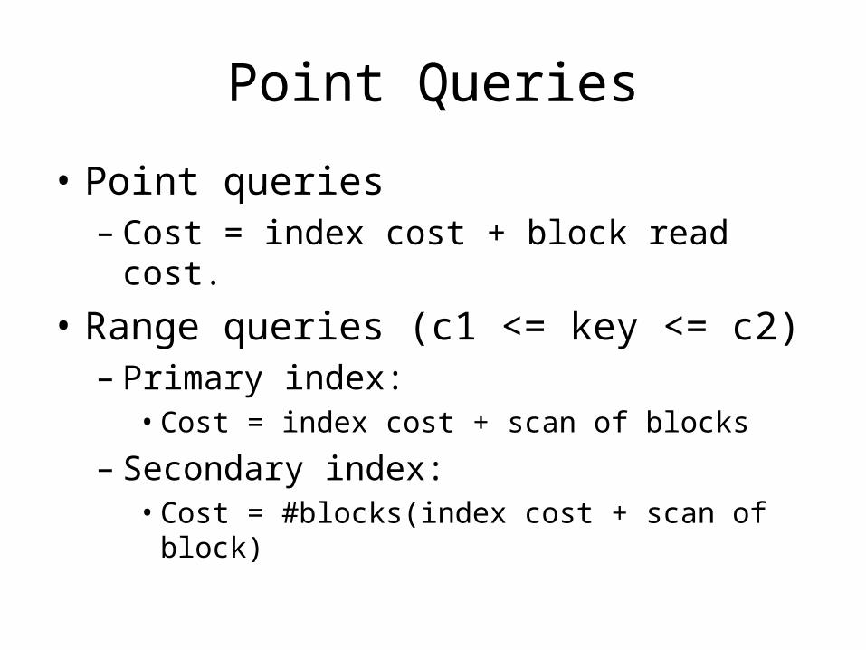
Point Queries

• Point queries– Cost = index cost + block read cost.

• Range queries (c1 <= key <= c2)– Primary index:

• Cost = index cost + scan of blocks

– Secondary index:• Cost = #blocks(index cost + scan of block)

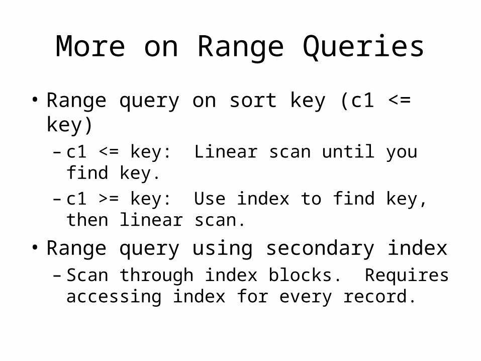
More on Range Queries

• Range query on sort key (c1 <= key)– c1 <= key: Linear scan until you find key.– c1 >= key: Use index to find key, then linear

scan.

• Range query using secondary index– Scan through index blocks. Requires

accessing index for every record.

More Complex Selections

• Conditions on multiple attributes• Negations• Disjunctions• Grouping pointers when selection is on

multiple attributes:– Find a set of solutions for each condition.– Either compute its union or intersection,

depending on the condition (disjunction or conjunction.)

Sorting

• Sorted relations are easier to scan.

• The cost of sorting a relation before querying it can be less than querying an unsorted relation.

• Two types of sorts:– In memory– Out of memory (a.k.a., external sorting)

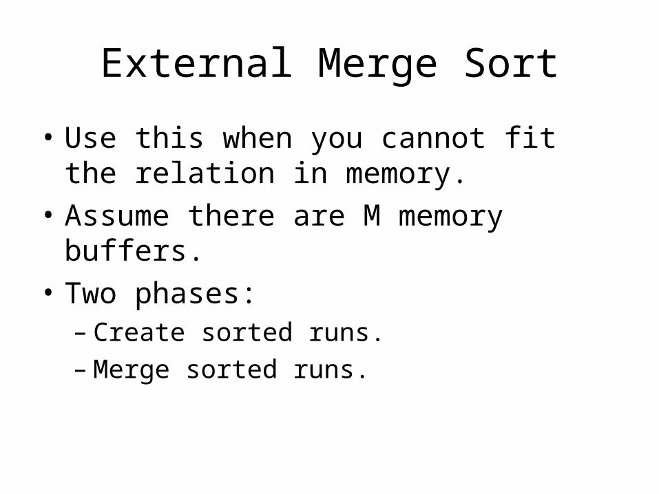
External Merge Sort

• Use this when you cannot fit the relation in memory.

• Assume there are M memory buffers.

• Two phases:– Create sorted runs.– Merge sorted runs.

External Merge Sort, Phase 1

• Fill the M memory buffers with the next M blocks of the relation.

• Sort the M blocks.

• Write the sorted blocks to disk.

External Merge Sort, Phase 2

• Assume there are at most M-1 runs.

• Read the first block of each run into memory.

• At each iteration, find the lowest record from the M-1 runs.

• Place it into the memory buffer.

• If any run is empty, read its next block.

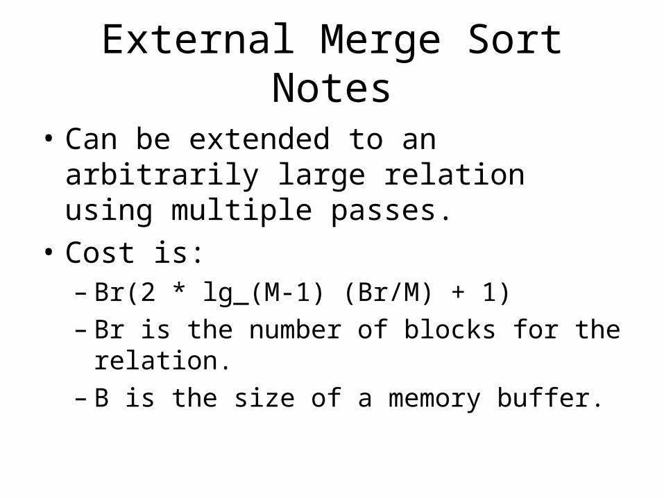
External Merge Sort Notes

• Can be extended to an arbitrarily large relation using multiple passes.

• Cost is:– Br(2 * lg_(M-1) (Br/M) + 1)– Br is the number of blocks for the relation.– B is the size of a memory buffer.

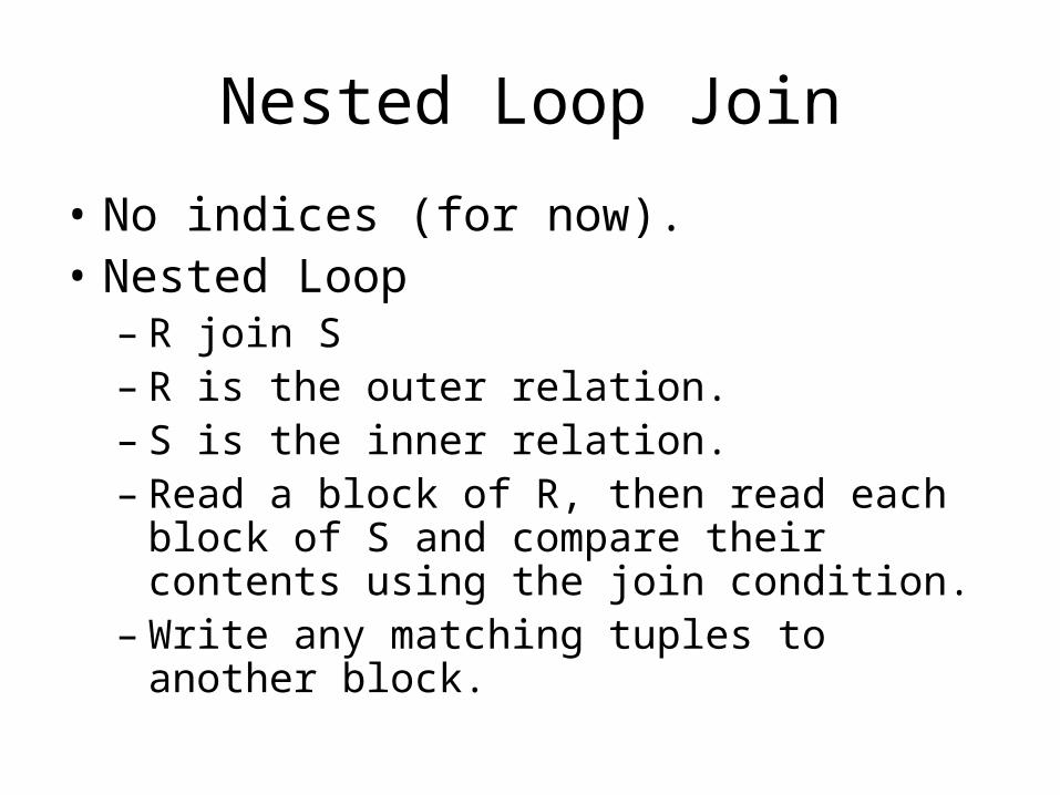
Nested Loop Join

• No indices (for now).• Nested Loop

– R join S– R is the outer relation.– S is the inner relation.– Read a block of R, then read each block of S

and compare their contents using the join condition.

– Write any matching tuples to another block.

Nested Loop Join Cost

• If you read tuple by tuple, it’s:– #tuples in R * #blocks in S + #blocks in R.

• Question: Which should be in inner relation, and which should be the outer?

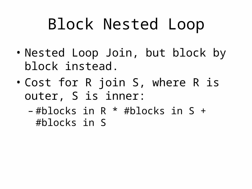
Block Nested Loop

• Nested Loop Join, but block by block instead.

• Cost for R join S, where R is outer, S is inner:– #blocks in R * #blocks in S + #blocks in S

Block Nested Loop Improvements

• Sorted relations?

• More memory?

Indexed Nested Loop Join

• Assume we have an index on a join attribute of one of the relations, R or S.

• Questions:– Which should the index be on?– Or, if both have indices on them, which should

be the outer one?

Indexed Nested Loop Join Cost

• #blocks in R + #rows in R * Ls– Ls is the cost of looking up a record in S using

the index.

More Joins

• Merge join– Sort R and S, and then merge them.

• Hash join– Hash R and S into buckets, and compare the

bucket contents.

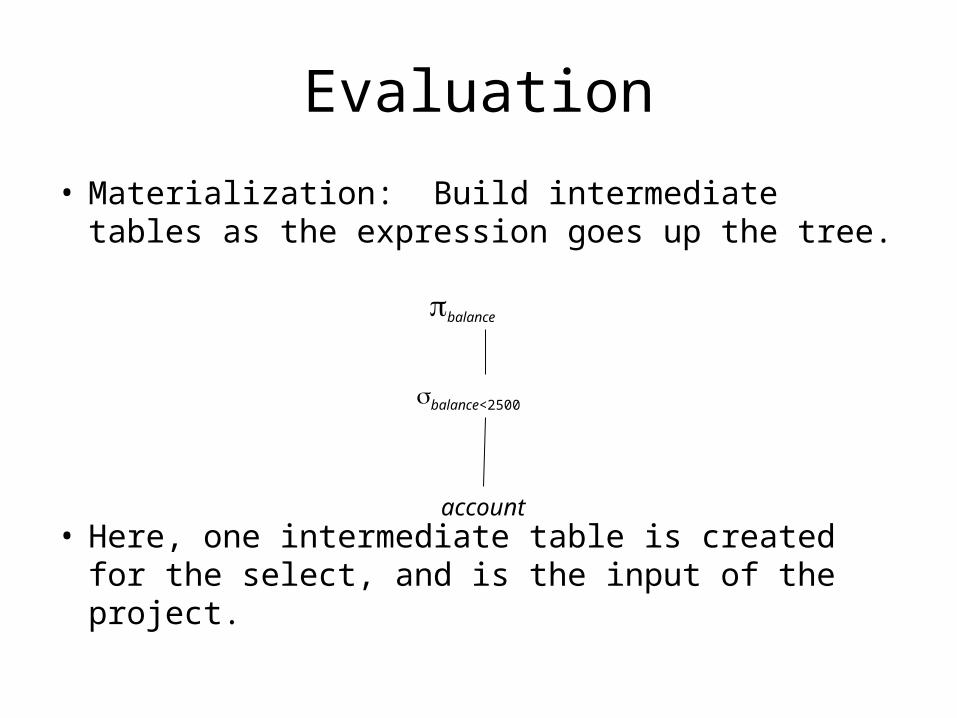
Evaluation

• Materialization: Build intermediate tables as the expression goes up the tree.

• Here, one intermediate table is created for the select, and is the input of the project.

balance

balance<2500

account

Materialization Cost

• Cost of writing out intermediate results to disk.

Pipelining

• Compute several operations simultaneously.

• As soon as a tuple is created from one operation, send it to the next. Here, send selected tuples straight to the projection.

balance

balance<2500

account

Implementation of Pipelining

• Requires buffers for each operation.

• Can be:– Demand driven – an operator must be asked

to generate a tuple.– Producer driven – an operator generates a

tuple whether its asked for or not.

Query Optimization

Some Actions of Query Optimization

• Reordering joins.

• Changing the positions of projects and selects.

• Changing the access structures used to read data.

Catalog Info

• Number of tuples in r.

• Number of blocks for r.

• Size of tuple of r.

• Blocking factor a r – the number of r tuples that fit in a block.

• The number of distinct values of each attribute of r.