r programming - guy lebanon's websitetheanalysisofdata.com/computing/r.pdf · 2018-05-06 · r...

Chapter 6

R Programming

6.1 R, Matlab, and Python

R is a programming language especially designed for data analysis and datavisualization. In some cases it is more convenient to use R than C++ or Java,making R an important data analysis tool. We describe below similarities anddi↵erences between R and its close relatives Matlab and Python.

R is similar to Matlab and Python in the following ways:

• They run inside an interactive shell in their default setting. In some casesthis shell is a complete graphical user interface (GUI).

• They emphasize storing and manipulating data as multidimensional arrays.

• They interface packages featuring functionalities, both generic, such as ma-trix operations, SVD, eigenvalues solvers, random number generators, andoptimization routines; and specialized, such as kernel smoothing and sup-port vector machines.

• They exhibit execution time slower than that of C, C++, and Fortran, andare thus poorly suited for analyzing massive1 data.

• They can interface with native C++ code, supporting large scale dataanalysis by implementing computational bottlenecks in C or C++.

The three languages di↵er in the following ways:

• R and Python are open-source and freely available for Windows, Linux,and Mac, while Matlab requires an expensive license.

• R, unlike Matlab, features ease in extending the core language by writingnew packages, as well as in installing packages contributed by others.

1The slowdown can be marginal or significant, depending on the program’s implementation.Vectorized code may improve computational e�ciency by performing basic operations on entirearrays rather than on individual array elements inside nested loops.

223

224 CHAPTER 6. R PROGRAMMING

• R features a large group of motivated contributors who enhance the lan-guage by implementing high-quality packages2.

• Developers designed R for statistics, yielding a syntax much better suitedfor computational data analysis, statistics, and data visualization.

• Creating high quality graphs in R requires less e↵ort than it does in Matlaband Python.

• R is the primary programming language in the statistics, biostatistics, andsocial sciences communities, while Matlab is the main programming lan-guage in engineering and applied math, and Python is a popular generalpurpose scripting and web development language.

6.2 Getting Started

The first step is to download and install a copy of R on your computer. R is avail-able freely for Windows, Linux, and Mac at the R Project website http://cran.r-project.org.

The two most common ways to run R are

• in a terminal prompt, by typing R in a Linux or Mac terminal, and

• inside a GUI, by double clicking the R icon on Windows or Mac or bytyping R -g Tk & on Linux.

Other ways to run R include

• using the Emacs Speaks Statistics (ESS) package from within Emacs,

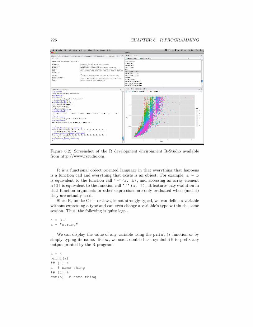
• using a third party GUI such as R-Studio (freely available fromhttp://www.rstudio.org; see Figure 6.2 for a screen shot), and

• running R from a client that accesses an R server application.

The easiest way to quit R is to type q() at the R prompt or to close the corre-sponding GUI window.

Like other programming languages, R code consists of a sequence of com-mands. Often, every command in R is typed in its own line. Alternatively,one line may contain multiple commands, separated by semicolons. Commentsrequire a hash sign # and occupy the remainder of the current line.

# This is a commenta = 4 # single statementa = 4; b = 3; c = b # multiple statements

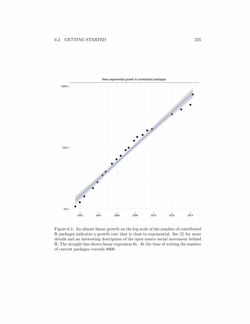
2Figure 6.1 demonstrates the rapid growth in the number of packages (see also [5]). Allcontributed packages go through a quality control process, and enforcement of standards, andhave common documentation format.

6.2. GETTING STARTED 225

●

●

●

●

●

●

●

●

●

●

●●

●

●●

●●

●

●

●

●

100

1000

10000

2002 2004 2006 2008 2010 2012 2014

Near exponential growth in contributed packages

Figure 6.1: An almost linear growth on the log scale of the number of contributedR packages indicates a growth rate that is close to exponential. See [5] for moredetails and an interesting description of the open source social movement behindR. The straight line shows linear regression fit. At the time of writing the numberof current packages exceeds 8000.


Figure 6.2: Screenshot of the R development environment R-Studio availablefrom http://www.rstudio.org.

R is a functional object oriented language in that everything that happensis a function call and everything that exists is an object. For example, a = bis equivalent to the function call ’=’(a, b), and accessing an array elementa[3] is equivalent to the function call ’[’(a, 3). R features lazy evalution inthat function arguments or other expressions are only evaluated when (and if)they are actually used.

Since R, unlike C++ or Java, is not strongly typed, we can define a variablewithout expressing a type and can even change a variable’s type within the samesession. Thus, the following is quite legal.

a = 3.2a = "string"

We can display the value of any variable using the print() function or bysimply typing its name. Below, we use a double hash symbol ## to prefix anyoutput printed by the R program.

a = 4print(a)## [1] 4a # same thing## [1] 4cat(a) # same thing

6.2. GETTING STARTED 227

## 4# cat can print multiple variables one after the othercat("The value of the variable a is: ", a)## The value of the variable a is: 4

As shown above, we set variables with the assignment operator =. An al-ternative is the operator <-, as in a <- 4 or 4 -> a. We use the classical =operator since it is more similar to assignment operators in other languages.

Strings in R are sequences of case sensitive characters surrounded by single ordouble quotes. To get help on a specific function, operator, or data object, typehelp(X) where X is the corresponding string. Similarly, example(X) showsan example of the use of the function X. The function help.start(X) startsan html-based documentation within a browser, which is sometimes easier tonavigate. Searching the help documentation using help.search(X) is usefulif you cannot recall the precise string on which you want to seek help. In additionto the commands above, searching the web using a search engine often providesuseful results.

In R, periods can be used to delimit words within a variable name; for ex-ample, my.parallel.clustering is a legitimate name for a variable or afunction. The $ operator in R has a similar role to the period operation in C++and Java.

Here are some important commands with short explanations.

x = 3 # assign value 3 to variable xy = 3*x + 2 # basic variable assignment and arithmeticratio.of.x.and.y = x / y # divide x by y and assign resultls() # list variable names in workspace memoryls(all.names = TRUE) # list all variables including hidden onesls.str() # print annotated list of variable namessave.image(file = "fname") # save all variables to a filesave(x, y, file = "fname") # save specified variablesrm(x, y) # clear variables x and y from memoryrm(list = ls()) # clear all variables in workspace memoryload(varFile) # load variables from file back to the workspacehistory(15) # display 15 most recent commands

The precise interaction of the command line or R IDE tool (like R-Studio)depends on the operating system and IDE program. In general, pressing the uparrow key and down arrow key allows browsing through the command historyfor previous commands. This can be very useful for fixing typos or for executingslight modifications of long commands. In the Linux and Mac terminal, Control-R takes a text pattern and returns the most recent command containing thatpattern.

Upon exiting R with the q() function, the command line prompts the userto save the workspace memory. Saving the workspace memory places all cur-rent variables in a file named .RData in the current directory. Launching Rautomatically uploads that file if it exists in the current directory, retrieving


the set of variables from the previous session in that directory. Inside R, theuser can change directories or view the current directory using setwd(X) andgetwd() respectively (X denotes a string containing a directory path). Thefunction system(X) executes the shell command X.

# change directory to home directorysetwd("˜")# display all files in current directorydir(path = ".", all.files = TRUE)# execute bash command ls -al (in Linux)system("ls -al")

As stated earlier, R features easy installation of both core R and third partypackages. The function install.packages(X) installs the functions anddatasets in the package X from the Internet. After installation the functionlibrary(X) brings the package into scope, thus making the functions andvariables in the package X available to the programmer. This two-stage pro-cess mitigates potential overlap in the namespaces of libraries. Typically, an Rprogrammer would install many packages3 on his or her computer, but haveonly a limited number in scope at any particular time. A list of availablepackages, their implementation and documentation is available at http://cran.r-project.org/web/packages/. These packages often contain interesting and demon-strative datasets. The function data lists the available datasets in a particularpackage.

# install package ggplot2install.packages("ggplot2")# install package from a particular mirror siteinstall.packages("ggplot2", repos="http://cran.r-project.org")# install a package from source, rather than binaryinstall.packages("ggplot2", type = "source")library('ggplot2') # bring package into scope# display all datasets in the package ggplot2data(package = 'ggplot2')installed.packages() # display a list of installed packagesupdate.packages() # update currently installed packages

R attempts to match a variable or function name by searching the currentworking environment followed by the packages that are in scope (loaded using thelibrary function) with the earliest match used if there are multiple matches.The function search displays the list of packages that are being searched fora match and the search order with the first entry defaulting to the workingenvironment, represented by .GlobalEnv. As a result, the working environmentmay mask variables or functions that are found further down the search path.

3The number of available packages is over 8000 in the year 2015; see Figure 6.1 for thegrowth trajectory.

6.3. SCALAR DATA TYPES 229

The code below demonstrates masking the variable pi by a global environ-ment variable with the value 3, and retrieving the original value after clearingit.

pi## [1] 3.141593pi = 3 # redefines variable pipi # .GlobalEnv match## [1] 3rm(pi) # removes masking variablespi## [1] 3.141593

The function sink(outputFile) records the output to the file outputFileinstead of the display, which is useful for creating a log-file for later examination.To print the output both to screen and to a file, use the following variation.

sink(file = 'outputFile', split = TRUE)

We have concentrated thus far on executing R code interactively. To executeR code written in a text file foo.R (.R is the conventional filename extensionfor R code) use either

• the R function source("foo.R"),

• the command R CMD BATCH foo.R from a Linux or Mac terminal, or

• the command Rscript foo.R from a linux or R terminal.

It is also possible to save the R code as a shell script file whose first linecorresponds to the location of the Rscript executable program, which in mostcases is the following line.

#!/usr/bin/Rscript

The file can then be executed by typing its name in the Linux or Mac OS ter-minal (assuming it has executable permission). This option has the advantageof allowing Linux style input and output redirecting via foo.R < inFile >outFile and other shell tricks.

The last three options permit passing parameters to the script, for example us-ing R CMD BATCH --args arg1 arg2 foo.R or Rscript foo.R arg1arg2. Calling commandArgs(TRUE) inside a script retrieves the commandline arguments as a list of strings.

6.3 Scalar Data Types

As we saw in the case of C++ and Java, a variable may refer to a scalar ora collection. Scalar types include numeric, integer, logical, string, dates, and


factors. Numeric and integer variables represent real numbers and integers, re-spectively. A logical or binary variable is a single bit whose value in R is TRUEor FALSE. Strings are ordered sequences of characters. Dates represent calendardates. Factor variables represent values from an ordered or unordered finite set.Some operations can trigger casting between the various types. Functions suchas as.numeric can perform explicit casting.

a = 3.2; b = 3 # double typesb## [1] 3typeof(b) # function returns type of object## [1] "double"c = as.integer(b) # cast to integer typec## [1] 3typeof(c)## [1] "integer"c = 3L # alternative to casting: L specifies integerd = TRUEd## [1] TRUEe = as.numeric(d) # casting to numerice## [1] 1f = "this is a string" # stringf## [1] "this is a string"ls.str() # show variables and their types## a : num 3.2## b : num 3## c : int 3## d : logi TRUE## e : num 1## f : chr "this is a string"

Factor variables assume values in a predefined set of possible values. Thecode below demonstrates the use of factors in R.

current.season = factor("summer",levels = c("summer", "fall", "winter", "spring"),ordered = TRUE) # ordered factor

current.season## [1] summer## 4 Levels: summer < fall < ... < springlevels(current.season) # display factor levels## [1] "summer" "fall" "winter" "spring"my.eye.color = factor("brown", levels = c("brown", "blue", "green"),

ordered = FALSE) # unordered factormy.eye.color

6.4. VECTORS, ARRAYS, LISTS, AND DATAFRAMES 231

## [1] brown## Levels: brown blue green

The value NA (meaning Not Available) denotes missing values. When de-signing data analysis functions, NA values should be carefully handled. Manyfunctions feature the argument na.rm which, if TRUE, operates on the dataafter removing any NA values.

6.4 Vectors, Arrays, Lists, and Dataframes

Vectors, arrays, lists, and dataframes are collections that hold multiple scalarvalues4. A vector is a one-dimensional ordered collection of variables of the sametype. An array is a multidimensional generalization of vectors of which a matrixis a two-dimensional special case. Lists are ordered collections of variables ofpotentially di↵erent types. The list signature is the ordered list of variable typesin the list. A dataframe is an ordered collection of lists having identical samesignature.

To refer to specific array elements use integers inside square brackets. Forexample A[3] refers to the third element and A[c(1, 2)] refers to the first twoelements. Negative integers inside the square bracket corresponds to a selectionof all elements except for the specified positions, for example A[-3] refers toall elements but the third one. It is also possible to refer to array elements bypassing a vector of boolean values with the selected elements corresponding tothe TRUE values. For example A[c(TRUE, TRUE, FALSE)] corresponds tothe third element. If the boolean vector is shorter than the array length it willbe recycled to be of the same length.

Below are some examples of creating and handling vectors and arrays.

# c() concatenates arguments to create a vectorx=c(4, 3, 3, 4, 3, 1)x## [1] 4 3 3 4 3 1length(x)## [1] 62*x+1 # element-wise arithmetic## [1] 9 7 7 9 7 3# Boolean vector (default is FALSE)y = vector(mode = "logical", length = 4)y## [1] FALSE FALSE FALSE FALSE# numeric vector (default is 0)z = vector(length = 3, mode = "numeric")z## [1] 0 0 0

4Formally, a numeric scalar in R is a vector of size 1 and thus it is not fundamentally di↵erentfrom a vector.


q = rep(3.2, times = 10) # repeat value multiple timesq## [1] 3.2 3.2 3.2 3.2 3.2 3.2 3.2 3.2 3.2 3.2w=seq(0, 1, by = 0.1) # values in [0,1] in 0.1 incrementsw## [1] 0.0 0.1 0.2 0.3 0.4 0.5 0.6 0.7 0.8 0.9## [11] 1.0# 11 evenly spaced numbers between 0 and 1w=seq(0, 1, length.out = 11)w## [1] 0.0 0.1 0.2 0.3 0.4 0.5 0.6 0.7 0.8 0.9## [11] 1.0# create an array with TRUE/FALSE reflecting whether condition holdsw <= 0.5## [1] TRUE TRUE TRUE TRUE TRUE TRUE## [7] FALSE FALSE FALSE FALSE FALSEany(w <= 0.5) # is it true for some elements?## [1] TRUEall(w <= 0.5) # is it true for all elements?## [1] FALSEwhich(w <= 0.5) # for which elements is it true?## [1] 1 2 3 4 5 6w[w <= 0.5] # extracting from w entries for which w<=0.5## [1] 0.0 0.1 0.2 0.3 0.4 0.5subset(w, w <= 0.5) # an alternative with the subset function## [1] 0.0 0.1 0.2 0.3 0.4 0.5w[w <= 0.5] = 0 # zero out all components smaller or equal to 0.5w## [1] 0.0 0.0 0.0 0.0 0.0 0.0 0.6 0.7 0.8 0.9## [11] 1.0

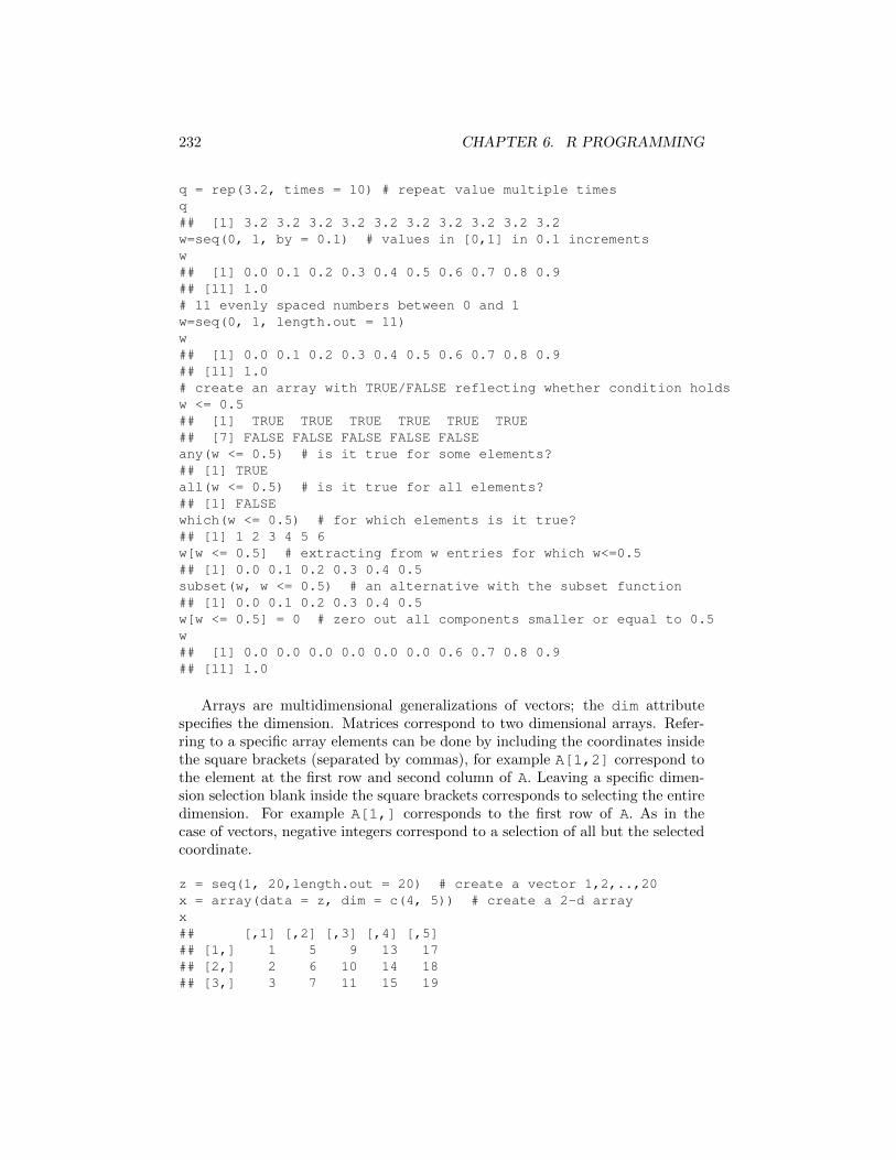
Arrays are multidimensional generalizations of vectors; the dim attributespecifies the dimension. Matrices correspond to two dimensional arrays. Refer-ring to a specific array elements can be done by including the coordinates insidethe square brackets (separated by commas), for example A[1,2] correspond tothe element at the first row and second column of A. Leaving a specific dimen-sion selection blank inside the square brackets corresponds to selecting the entiredimension. For example A[1,] corresponds to the first row of A. As in thecase of vectors, negative integers correspond to a selection of all but the selectedcoordinate.

z = seq(1, 20,length.out = 20) # create a vector 1,2,..,20x = array(data = z, dim = c(4, 5)) # create a 2-d arrayx## [,1] [,2] [,3] [,4] [,5]## [1,] 1 5 9 13 17## [2,] 2 6 10 14 18## [3,] 3 7 11 15 19


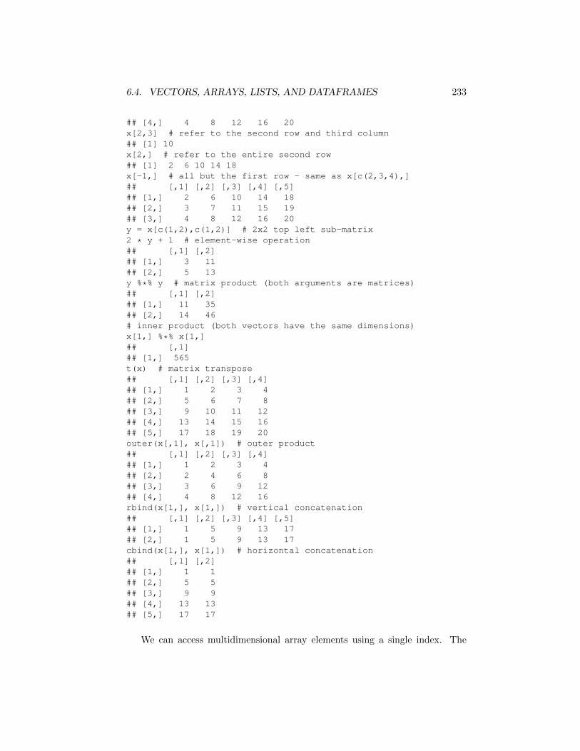
## [4,] 4 8 12 16 20x[2,3] # refer to the second row and third column## [1] 10x[2,] # refer to the entire second row## [1] 2 6 10 14 18x[-1,] # all but the first row - same as x[c(2,3,4),]## [,1] [,2] [,3] [,4] [,5]## [1,] 2 6 10 14 18## [2,] 3 7 11 15 19## [3,] 4 8 12 16 20y = x[c(1,2),c(1,2)] # 2x2 top left sub-matrix2 * y + 1 # element-wise operation## [,1] [,2]## [1,] 3 11## [2,] 5 13y %*% y # matrix product (both arguments are matrices)## [,1] [,2]## [1,] 11 35## [2,] 14 46# inner product (both vectors have the same dimensions)x[1,] %*% x[1,]## [,1]## [1,] 565t(x) # matrix transpose## [,1] [,2] [,3] [,4]## [1,] 1 2 3 4## [2,] 5 6 7 8## [3,] 9 10 11 12## [4,] 13 14 15 16## [5,] 17 18 19 20outer(x[,1], x[,1]) # outer product## [,1] [,2] [,3] [,4]## [1,] 1 2 3 4## [2,] 2 4 6 8## [3,] 3 6 9 12## [4,] 4 8 12 16rbind(x[1,], x[1,]) # vertical concatenation## [,1] [,2] [,3] [,4] [,5]## [1,] 1 5 9 13 17## [2,] 1 5 9 13 17cbind(x[1,], x[1,]) # horizontal concatenation## [,1] [,2]## [1,] 1 1## [2,] 5 5## [3,] 9 9## [4,] 13 13## [5,] 17 17

We can access multidimensional array elements using a single index. The


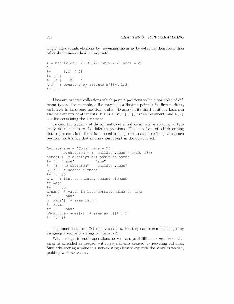
single index counts elements by traversing the array by columns, then rows, thenother dimensions where appropriate.

A = matrix(c(1, 2, 3, 4), nrow = 2, ncol = 2)A## [,1] [,2]## [1,] 1 3## [2,] 2 4A[3] # counting by columns A[3]=A[1,2]## [1] 3

Lists are ordered collections which permit positions to hold variables of dif-ferent types. For example, a list may hold a floating point in its first position,an integer in its second position, and a 3-D array in its third position. Lists canalso be elements of other lists. If L is a list, L[[i]] is the i-element, and L[i]is a list containing the i element.

To ease the tracking of the semantics of variables in lists or vectors, we typ-ically assign names to the di↵erent positions. This is a form of self-describingdata representation: there is no need to keep meta data describing what eachposition holds since that information is kept in the object itself.

L=list(name = 'John', age = 55,no.children = 2, children.ages = c(15, 18))

names(L) # displays all position names## [1] "name" "age"## [3] "no.children" "children.ages"L[[2]] # second element## [1] 55L[2] # list containing second element## $age## [1] 55L$name # value in list corresponding to name## [1] "John"L['name'] # same thing## $name## [1] "John"L$children.ages[2] # same as L[[4]][2]## [1] 18

The function uname(X) removes names. Existing names can be changed byassigning a vector of strings to names(X).

When using arithmetic operations between arrays of di↵erent sizes, the smallerarray is extended as needed, with new elements created by recycling old ones.Similarly, storing a value in a non-existing element expands the array as needed,padding with NA values.


a = c(1, 2)b = c(10, 20, 30, 40, 50)a + b## [1] 11 22 31 42 51b[7] = 70b## [1] 10 20 30 40 50 NA 70

A dataframe is an ordered sequence of lists sharing the same signature. Adataframe often serves as a table whose rows correspond to data examples (sam-ples from a multivariate distribution) and whose columns correspond to dimen-sions or features.

vecn = c("John Smith","Jane Doe")veca = c(42, 45)vecs = c(50000, 55000)R = data.frame(name = vecn, age = veca, salary = vecs)R## name age salary## 1 John Smith 42 50000## 2 Jane Doe 45 55000names(R) = c("NAME", "AGE", "SALARY") # modify column namesR## NAME AGE SALARY## 1 John Smith 42 50000## 2 Jane Doe 45 55000

The core R package datasets contains many interesting and demonstrativedatasets, such as the iris dataset, whose first four dimensions are numericmeasurements describing flower geometry, and whose last dimension is a stringdescribing the flower species.

names(iris) # lists the dimension (column) names## [1] "Sepal.Length" "Sepal.Width"## [3] "Petal.Length" "Petal.Width"## [5] "Species"head(iris, 4) # show first four rows## Sepal.Length Sepal.Width Petal.Length## 1 5.1 3.5 1.4## 2 4.9 3.0 1.4## 3 4.7 3.2 1.3## 4 4.6 3.1 1.5## Petal.Width Species## 1 0.2 setosa## 2 0.2 setosa## 3 0.2 setosa## 4 0.2 setosairis[1,] # first row


## Sepal.Length Sepal.Width Petal.Length## 1 5.1 3.5 1.4## Petal.Width Species## 1 0.2 setosairis$Sepal.Length[1:10] # sepal length of first ten samples## [1] 5.1 4.9 4.7 4.6 5.0 5.4 4.6 5.0 4.4 4.9# allow replacing iris$Sepal.Length with the shorter Sepal.Lengthattach(iris, warn.conflicts = FALSE)mean(Sepal.Length) # average of Sepal.Length across all rows## [1] 5.843333colMeans(iris[,1:4]) # means of all four numeric columns## Sepal.Length Sepal.Width Petal.Length## 5.843333 3.057333 3.758000## Petal.Width## 1.199333

The subset function is useful for extracting subsets of a dataframe.

# extract all rows whose Sepal.Length variable is less than 5# and whose species is not setosasubset(iris, Sepal.Length < 5 & Species != "setosa")## Sepal.Length Sepal.Width Petal.Length## 58 4.9 2.4 3.3## 107 4.9 2.5 4.5## Petal.Width Species## 58 1.0 versicolor## 107 1.7 virginica# count number of rows corresponding to setosa speciesdim(subset(iris, Species == "setosa"))[1]## [1] 50

The function summary provides a useful statistical summary of the di↵erentdataframe columns. R automatically determines whether the variables are nu-meric, such as Sepal.Length, or factors, such as Species. For numeric vari-ables, the summary function displays the minimum, maximum, mean, median,and the 25% and 75% percentiles. For factor variables, the summary functiondisplays the number of dataframe rows in each of the factor levels.

summary(iris)## Sepal.Length Sepal.Width## Min. :4.300 Min. :2.000## 1st Qu.:5.100 1st Qu.:2.800## Median :5.800 Median :3.000## Mean :5.843 Mean :3.057## 3rd Qu.:6.400 3rd Qu.:3.300## Max. :7.900 Max. :4.400## Petal.Length Petal.Width## Min. :1.000 Min. :0.100

6.5. IF-ELSE, LOOPS, AND FUNCTIONS 237

## 1st Qu.:1.600 1st Qu.:0.300## Median :4.350 Median :1.300## Mean :3.758 Mean :1.199## 3rd Qu.:5.100 3rd Qu.:1.800## Max. :6.900 Max. :2.500## Species## setosa :50## versicolor:50## virginica :50######

With appropriate formatting, we can create a dataframe using a text file. Forexample, we can load the following text file containing data into a dataframe inR using the read.table(X, header=TRUE) function (use header=FALSEif there is no header line containing column names).

Sepal.Length Sepal.Width Petal.Length Petal.Width Species5.1 3.5 1.4 0.2 setosa4.9 3.0 1.4 0.2 setosa

# read text file into dataframeIris=read.table('irisFile.txt', header = TRUE)# same but from Internet locationIris=read.table('http://www.exampleURL.com/irisFile.txt',

header = TRUE)

We can examine and edit dataframes and other variables within a text editoror a spreadsheet-like environment using the edit function.

edit(iris) # examine data as spreadsheetiris = edit(iris) # edit dataframe/variablenewIris = edit(iris) # edit dataframe/variable but keep original

6.5 If-Else, Loops, and Functions

The flow of control of R code is very similar to that of other programming lan-guages. Below are some examples of if-else, loops, function definitions, and func-tion calls.

a = 10; b = 5; c = 1if (a < b) {

d = 1} else if (a == b) {


d = 2} else {

d = 3}d## [1] 3

The logical operators in R are similar to those in C++ and Java. Examplesinclude && for AND, || for OR, == for equality, and != for inequality.

For-loops repeat for a pre-specified number of times, with each loop assigninga di↵erent component of a vector to the iteration variable. Repeat-loops repeatuntil a break statement occurs. While-loops repeat until a break statementoccurs or until the loop condition is not satisfied. The next statement abortsthe current iteration and proceeds to the next iteration.

sm=0# repeat for 100 iteration, with num taking values 1:100for (num in seq(1, 100, by = 1)) {

sm = sm + num}sm # same as sum(1:100)## [1] 5050repeat {

sm = sm - numnum = num - 1if (sm == 0) break # if sm == 0 then stop the loop

}sm## [1] 0a = 1; b = 10# continue the loop as long as b > awhile (b>a) {

sm = sm + 1a = a + 1b = b - 1

}sm## [1] 5

Functions in R are similar to those in C++ and Java. When calling a func-tion the arguments flow into the parameters according to their order at the callsite. Alternatively, arguments can appear out of order if the calling environmentprovides parameter names.

# parameter bindings by orderfoo(10, 20, 30)# (potentially) out of order parameter bindingsfoo(y = 20, x = 10, z = 30)

6.5. IF-ELSE, LOOPS, AND FUNCTIONS 239

Omitting an argument assigns the default value of the corresponding param-eter.

# passing 3 parametersfoo(x = 10, y = 20, z = 30)# x and y are missing and are assigned default valuesfoo(z = 30)# in-order parameter binding with last two parameters missingfoo(10)

Out of order parameter bindings and default values simplify calling functionswith long lists of parameters, when many of parameters take default values.

# myPower(.,.) raises the first argument to the power of the# second. The first argument is named bas and has default value 10.# The second parameter is named pow and has default value 2.myPower = function(bas = 10, pow = 2) {

res=bas ˆ pow # raise base to a powerreturn(res)

}myPower(2, 3) # 2 is bound to bas and 3 to pow (in-order)## [1] 8# same binding as above (out-of-order parameter names)myPower(pow = 3, bas = 2)## [1] 8myPower(bas = 3) # default value of pow is used## [1] 9

Since R passes variables by value, changing the passed arguments inside thefunction does not modify their respective values in the calling environment. Vari-ables defined inside functions are local, and thus are unavailable after the functioncompletes its execution. The returned value is the last computed variable or theone specified in a return function call. Returning multiple values can be doneby returning a list or a dataframe.

x = 2myPower2 = function(x) {x = xˆ2; return(x)}y = myPower2(x) # does not change x outside the functionx## [1] 2y## [1] 4

It is best to avoid loops when programming in R. There are two reasonsfor this: simplifying code and computational speed-up. Many mathematicalcomputations on lists, vectors, or arrays may be performed without loops usingcomponent-wise arithmetic. The code example below demonstrates the compu-tational speedup resulting from replacing a loop with vectorized code.


a = 1:10# compute sum of squares using a for loopsc = 0for (e in a) c = c + eˆ2c## [1] 385# same operation using vector arithmeticsum(aˆ2)## [1] 385# time comparison with a million elementsa = 1:1000000; c = 0system.time(for (e in a) c = c+eˆ2)## user system elapsed## 0.515 0.007 0.522system.time(sum(aˆ2))## user system elapsed## 0.006 0.002 0.008

Another way to avoid loops is to use the function sapply, which applies afunction passed as a second argument to the list, data-frame, or vector that ispassed as a first argument. This leads to simplified code, though the computa-tional speed-up may not apply in the same way as it did above.

a = seq(0, 1 ,length.out = 10)b = 0c = 0for (e in a) {

b = b + exp(e)}b## [1] 17.33958c = sum(sapply(a, exp))c## [1] 17.33958# sapply with an anonymous function f(x)=exp(xˆ2)sum(sapply(a, function(x) {return(exp(xˆ2))}))## [1] 15.07324# or more simplysum(sapply(a, function(x) exp(xˆ2)))## [1] 15.07324

6.6 Interfacing with C++ Code

R is inherently an interpreted language; that is, R compiles each command atrun time, resulting in many costly context switches and di�culty in applyingstandard compiler optimization techniques. Thus, R programs likely will not

6.6. INTERFACING WITH C++ CODE 241

execute as e�ciently as compiled programs5 in C, C++, or Fortran.The computational slowdown described above typically increases with the

number of elementary function calls or commands. For example, R code thatgenerates two random matrices, multiplies them, and then computes eigenvaluestypically will not su↵er a significant slowdown compared to similar implementa-tions in C, C++, or Fortran. The reason is that that such R code calls routinesthat are programmed in FORTRAN or C++. On the other hand, R code contain-ing many nested loops is likely to be substantially slower due to the interpreteroverhead.

For example, consider the code below, which compares two implementationsof matrix multiplication. The first uses R’s internal matrix multiplication andthe second implements it through three nested loops, each containing a scalarmultiplication.

n = 100; nsq = n*n# generate two random matricesA = matrix(runif(nsq), nrow = n, ncol = n)B = matrix(runif(nsq), nrow = n, ncol = n)system.time(A%*%B) # built-in matrix multiplication## user system elapsed## 0.001 0.000 0.001matMult=function(A, B, n) {

R=matrix(data = 0, nrow = n, ncol = n)for (i in 1:n)

for (j in 1:n)for (k in 1:n)

R[i,j]=R[i,j]+A[i,k]*B[k,j]return(R)

}# nested loops implementationsystem.time(matMult(A, B, n))## user system elapsed## 2.725 0.044 398.295

The first matrix multiplication is faster by several orders of magnitude evenfor a relatively small n = 100. The key di↵erence is that the built-in matrixmultiplication runs compiled C code.

Clearly, it is better, if possible, to write R code containing relatively fewloops and few elementary R functions. Since core R contains a rich library ofelementary functions, one can often follow this strategy. In some cases, however,this approach is not possible. A useful heuristic in this case is to identify com-putational bottlenecks using a profiler, then re-implement the o↵ending R codein a compiled language such as C or C++. The remaining R code will interfacewith the reimplemented bottleneck code via an external interface. Assuming thata small percent of the code is responsible for most of the computational ine�-

5R does have a compiler that can compile R code to native code, but the resulting speedupis not very high.


ciency (as is often the case), this strategy can produce substantial speedups withrelatively little e↵ort.

We consider two techniques for calling compiled C/C++ code from R: the sim-pler .C function and the more complex .Call function. In both cases, we com-pile C/C++ code using the terminal command R CMD SHLIB foo.c, which in-vokes the C++ compiler and create a foo.so file containing the compiled code.The .so file can be loaded within R using the function dynload(’foo.so’)and then called using the functions .C(’foo’, ...) or .Call(’foo’,...) (the remaining arguments contain R vectors, matrices, or dataframes thatwill be converted to pointers within the C/C++ code.

For example, consider the task of computingPn

j=1(aj + i)bj for all i, j =1, . . . , n given two vectors a and b of size n. The C code to compute the resultappears below. The first two pointers point to arrays containing the vectors a

and b, the third pointer points to the length of the arrays, and the last pointerpoints to the area where the results should appear. Note the presence of thepre-processor directive include<R.h>.

#include <R.h>#include <math.h>

void fooC(double* a, double* b, int* n, double* res) {int i, j;for (i = 0;i < (*n); i++) {

res[i] = 0;for (j = 0;j < (*n); j++)res[i] += pow(a[j] + i + 1, b[j]);

}}

Saving the code above as the file fooC.c and compiling using the terminalcommand below produces the file fooC.so that can be linked to an R sessionwith the dynload function.

R CMD SHLIB fooC.c

dyn.load("fooC.so") # load the compiled C codeA = seq(0, 1, length = 10)B = seq(0, 1, length = 10)C = rep(0, times = 10)L = .C("fooC", A, B, as.integer(10), C)ResC=L[[4]] # extract 4th list element containing resultResC## [1] 13.34392 17.48322 21.21480 24.70637## [5] 28.03312 31.23688 34.34390 37.37199## [9] 40.33396 43.23936fooR = function(A, B, n) {

res = rep(0, times = n)

6.6. INTERFACING WITH C++ CODE 243

for (i in 1:n)for (j in 1:n)

res[i] = res[i]+(A[j]+i)ˆ(B[j])return(res)

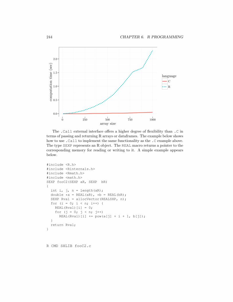
}ResR=fooR(A, B, 10)ResR## [1] 13.34392 17.48322 21.21480 24.70637## [5] 28.03312 31.23688 34.34390 37.37199## [9] 40.33396 43.23936sizes = seq(10, 1000, length = 10)Rtime = rep(0, 10)Ctime = Rtimei = 1for (n in sizes) {

A = seq(0, 1,length = n)B = seq(0, 1,length = n)C = rep(0, times = n)Ctime[i] = system.time(.C("fooC", A, B, as.integer(n), C))Rtime[i] = system.time(fooR(A, B, n))i = i+1

}DF = stack(list(C = Ctime, R = Rtime))names(DF) = c("system.time", "language")DF$size = sizes# plot run time as a function of array size for R and# .C implementationsqplot(x = size,

y = system.time,lty = language,

color = language,data = DF,size = I(1.5),

geom = "line",xlab = "array size",

ylab = "computation time (sec)")


0.0

0.5

1.0

1.5

2.0

0 250 500 750 1000

array size

computation

time(sec)

language

C

R

The .Call external interface o↵ers a higher degree of flexibility than .C interms of passing and returning R arrays or dataframes. The example below showshow to use .Call to implement the same functionality as the .C example above.The type SEXP represents an R object. The REAL macro returns a pointer to thecorresponding memory for reading or writing to it. A simple example appearsbelow.

#include <R.h>#include <Rinternals.h>#include <Rmath.h>#include <math.h>SEXP fooC2(SEXP aR, SEXP bR){

int i, j, n = length(aR);double *a = REAL(aR), *b = REAL(bR);SEXP Rval = allocVector(REALSXP, n);for (i = 0; i < n; i++) {

REAL(Rval)[i] = 0;for (j = 0; j < n; j++)REAL(Rval)[i] += pow(a[j] + i + 1, b[j]);

}return Rval;

}

R CMD SHLIB fooC2.c

6.7. CUSTOMIZATION 245

dyn.load("fooC2.so") # load the compiled C codeA = seq(0, 1, length = 10)B = seq(0, 1, length = 10).Call("fooC2", A, B)

6.7 Customization

When R starts it executes the function .First in the .Rprofile file in theuser’s home directory (if it exists). This is a good place to put user preferredoptions. Similarly, R executes the function .Last in the same file at the end ofany R session. The function options adjust the behavior of R in many ways, forexample to include more digits when displaying the value of a numeric variable.

Below are two very simple .First and .Last functions.

.First = function() {options(prompt = 'R >', digits = 6)library('ggplot2')

}.Last = function() {

cat(date(), 'Bye')}

In Linux or Mac, we can execute R with flags; for example, R -q starts Rwithout printing the initial welcome message.

6.8 Notes

R programming books include free resources such as the o�cial introductionto R manual http://cran.r-project.org/doc/manuals/R-intro.html (replace htmlwith pdf for pdf version) and the language reference http://cran.r-project.org/doc/manuals/R-lang.html (replace html with pdf for pdf version). Additionalmanuals on writing R extensions, importing data, and other topics are availableat http://cran.r-project.org/doc/manuals/. Many additional books are availablevia commercial publishers.

R packages are available from http://cran.r-project.org. Each package fea-tures a manual in a common documentation format; many packages feature ad-ditional tutorial documents known as vignettes. Navigating the increasing repos-itory of packages can be overwhelming. The Task Views help to aggregate listsof packages within a particular task or area. The list of Task Views is available athttp://cran.r-project.org/web/views/. Another useful tool is http://crantastic.orgwhich shows recently contributed or updated packages, user reviews, and ratings.Finally, the freely available R-Journal at http://journal.r-project.org/ containshigh quality refereed articles on the R language, including many descriptions ofcontributed packages.


TheWriting R Extensions manual (http://cran.r-project.org/doc/manuals/R-exts.pdf) contains more information on the .C and .Call external interfaces.The Rcpp package o↵ers a higher degree of flexibility for interfacing C++ codeand enables using numeric C++ libraries such as GSL, Eigen, and Armadillo.

6.9 Exercises

1. Type the R code in this chapter into an R session and observe the results.

2. Implement a function that computes the log of the factorial value of aninteger using a for loop. Note that implementing it using log(A)+log(B)+· · · avoids overflow while implementing it as log(A · B · · · · ) creates anoverflow early on.

3. Implement a function that computes the log of the factorial value of aninteger using recursion.

4. Using your two implementations of log-factorial in (2) and (3) above, com-pute the sum of the log-factorials of the integers 1, 2, . . . , N for various Nvalues.

5. Compare the execution times of your two implementations for (4) with animplementation based on the o�cial R function lfactorial(n). Youmay use the function system.time() to measure execution time. Whatare the growth rates of the three implementations as N increases? Use thecommand options(expressions=500000) to increase the number ofnested recursions allowed. Compare the timing of the recursion implemen-tation as much as possible, and continue beyond that for the other twoimplementations.

r programming - guy lebanon's websitetheanalysisofdata.com/computing/r.pdf · 2018-05-06 · r...

Documents