?r=20020050260 2018-02 · pdf file · 2013-08-30performance data gathering and...

._ _ jj(z e_

Performance Data Gathering and Representation

from Fixed-Size Statistical Data

Jerry C. Yan, Haoqiang H. Jin, and Melisa A. Schmidt

{.van, hjin, schmidt}@nas.nasa.gov

NASA Ames Research Center, Moffett Field, CA 94035

Abstract

The two commonly-used performance data types in the super-computing commu-

nity, statistics and event traces, are discussed and compared. Statistical data are

much more compact but lack the probative power event traces offer. Event traces,

on the other hand, are unbounded and can easily fill up the entire file system during

program execution. In this paper, we propose an innovative methodology for per-

formance data gathering and representation that offers a middle ground. Two basic

ideas are employed: the use of averages to replace recording data for each instance

and "formulae" to represent sequences associated with communication and control

flow. The user can trade off tracing overhead, trace data size with data quality in-

crementally. In other words, the user will be able to limit the amount of trace data

collected and, at the same time, carry out some of the analysis event traces offer

using space-time views. With the help of a few simple examples, we illustrate the

use of these techniques in performance tuning and compare the quality of the traces

we collected with event traces. We found that the trace files thus obtained are, in-

deed, small, bounded and predictable before program execution, and that the quality

of the space-time views generated from these statistical data are excellent. Further-

more, experimental results showed that the formulae proposed were able to capture

all the sequences associated with 11 of the 15 applications tested. The performance

of the formulae can be incrementally improved by allocating more memory at run-

time to learn longer sequences.

1. Introduction

Computing today increasingly depends on the effective utilization of multiprocessors. Systems

currently available range from those with tightly-coupled processors to those with a network of

workstations. Innovation in hardware technologies continuously reduce the communication time

between processing nodes as well as access latencies across the memory hierarchy to support

computing in this new environment. Unfortunately, the software infrastructure (e.g. program-

ming languages, compiler_, operating systems, and performance monitoring and prediction tools)

of 25

https://ntrs.nasa.gov/search.jsp?R=20020050260 2018-05-25T18:05:51+00:00Z

availabletodaystill hasnotkeptpacewith thestate-of-the-artmultiprocessinghardware[Pan91,

SMS95]. In particular, the lack of useful, accurate facilities for measuring and analyzing program

performance is particularly distressing, since performance is the raison d'etre for parallelism.

1.1 Performance Analysis Systems

Traditional performance-analysis systems (e.g. gproj) that generate textual information have

proven quite effective for sequential programs. Metrics based on the distribution of elapsed time

across the program can systematically direct the user towards time consuming regions of code

where performance should be improved. Unfortunately, such simple measures are insufficient

for parallel programs and may even be misleading [HIM91]. This problem arises primarily be-

cause aggregate values do not necessarily capture the dynamic interactions between various proc-

esses (and processing nodes) involved in the computation. In order to fully understand the

performance of a particular program on a particular machine, a performance tool must capture

and analyze dynamic execution characteristics.

Visualization has been used extensively to represent simulation results for many complex physi-

cal systems. In the past five years, the application of visualization technologies to manage the

vast amount of performance data collected in multiprocessors has also been proposed. Many

tools supporting performance visualization are available today, either in the public domain (e.g.

AlMS [YSM95], Pablo [RO*91], Paradyn [MC'95], and ParaGraph [HE91]) or as part of a

multiprocessor's system software (e.g. CXTRACE on Convex's SPP-1, ParAid on Intel's Para-

gon, MPP Apprentice on CRI's T3D, PRISM on TMC's CM5, and PV on IBM's SP2). Typi-

cally, performance data are displayed post-mortem. These displays provide valuable feed-back

about users' choice of parallel algorithm, strategies for load balancing and data distribution, as

well as how the application will scale with increasing numbers of processing nodes and problem

sizes. A good survey of some state-of-the-art research efforts can be found in [PMY95, SK90].

1.2 Statistics vs. Event Traces: A Comparison

Broadly speaking, there are two kinds of performance data: statistics and event traces. Statistics

are concerned with counts and duration: e.g. how many times a procedure has been called and, on

average, how long it took to complete. Event traces, on the other hand, record the exact sequence

(and in most cases, the actual time) of actions that took place during program execution. Fur-

thermore, when the clocks across processing nodes are synchronized, event traces can help pro-

vide a global picture of what took place (e.g. how long a message took to reach node b from node

a). As of today, all the trace tools that animate parallel program execution (e.g. using space-time

diagrams) require synchronized event traces from multiple nodes.

of 25

Onemightsuggestthateventtracesshouldalwaysbegatheredsincethey containmuchmorein-formation.Unfortunately,eventtracesingeneralarelargeandthesizeof thetracefile is not pre-dictablebeforeprogramexecution.Furthermore,the collectionprocessitself is expensiveand

requiresalot of resources.Themostintrusiveactivity to supporteventtracesinvolvestheneedto allocatememorybuffer_dynamicallyin orderto savethe performancedataand flushingtodisk whenthesebuffersmefull. In fact,two commercialvendors(CRI's MPP-Apprentice and

TMC's PRISM) have opted not to support event traces, possibly to avoid excessive perturbation

on observed program behavior. In both cases, the user locates bottlenecks by studying the

amount of time a procedure or source line consumes and the activity that took place during this

time. The reasons so many other vendors (e.g. CXTRACE on Convex's SPP-1, ParAid on Intel's

Paragon, and PVon IBM's SP2) are still supporting event tracing can probably be explained by

the differences of the two representations as discussed below.

a) The fact that

nodec is "behind" node_nodea and nodeb is

only visible on the nodeb

space-time view nodec

Procedure A

vn idle time

• Procedure B

b) The fact that nodea

communication nodeboverlaps computa-tion is only visible on nodec

the space-time view

Space-time view

Elapsed Time

-timetview

i

Elapsed Time w-

®A.e

E

E° _,_

o)

_k Histogram

nodea eb nodec

nodea nodeb nodec

Figure 1. Comparing space-time views vs. histograms in their abilities to capture pro-

gram behavior in 2 cases: a) computation/communication overlap, and b) load-imbalance.

Figure 1 compares the abilities of two visual representations supporting parallel program behav-

ior analysis, histograms vs. space-time views. Two interesting parallel program behavior patterns

involve synchronized behavior across nodes and communication-computation overlap. In the

space-time views shown on the left of Figure 1, each horizontal bar indicates activity that took

place at a node during a given time interval. "White spaces" indicate idleness, possibly waiting

for the arrival of a message. Messages are indicated as lines drawn from the sender node to the

receiver node. Each column of the histograms on the right plots accumulated time for various ac-

of 25

tivitiesfor thecorrespondingnode. Basically,nodea,nodeb,andnodecwereall executingProce-

dure A at the beginning of the time interval being monitored. In Figure 1a, nodes exchanged mes-

sages in a cyclic pattern. The fact that nodec was "behind" nodea and nodeb is only visible on the

space-time view. In Figure lb however, after Procedure A terminated, nodeb sent messages to

nodea and nodec before they all entered Procedure B. Although the user may suspect the exis-

tence of load imbalance based on the histogram, the fact that communication overlaps computa-

tion is only visible on the space-time view.

Table 1 gives a more detailed comparison between statistics and event traces in three areas: col-

lection requirements, trace file size and analyses these traces support. Two observations need to

be highlighted:

1. Event traces are relatively larger and unbounded. This can be a severe problem in practice.

2. Event traces support a much richer variety of analyses critical towards understanding the

behavior of parallel programs.

It is, therefore, not surprising that a lot of tools available today are still based on event traces.

1.3 Trace File Reduction Attempts

As mentioned above, event traces contain much richer information, but unfortunately the size of

a trace file is unbounded. Attempts have been made to reduce trace file size. In the Automated

Instrumentation and Monitoring System (AIMS) [YSM95] that was developed at NASA Ames

Research Center, two techniques for trace file reduction had been considered:

1. Merging trace records that always occur in pairs:

a) Message (e.g. send, receive, broadcast) blocking and unblocking.

b) Code-block (e.g. procedure, loop) entry and exit.

2. Using binary encoding for trace records.

In the first technique, a new trace record type was defined and used in place of two individual

records to eliminate some duplicate fields (e.g. the message type, size, and, tag). Our studies indi-

cated that trace record merging resulted in a reduction of 27% of the number of trace records,

which translated to an average reduction of 38% in actual trace file length in ASCII. Binary trace

encoding is the second technique to reduce trace file size. Researchers working on Pablo [RO*91]

reported 40% savings with the use of binary (vs. ASCII) representation. Our own calculations

also indicated similar savings (from 40% to 50%).

In summary, the trace file would only shrink by a factor of 4 even if both techniques were ap-

plied simultaneously. This was insufficient because applications of interests will scale up an or-

der of magnitude in problem size as well as number of nodes. Furthermore, no matter how

compact the representation may become, the generation of event traces leaves the trace file length

of 25

unbound.A fundamentalre-thinkingof theprocessof performanceinstrumentation,monitoringandtracerepresentationis requiredinorderto limit tracefile lengthwhilepreservingtherich con-tentavailableineventtraces.

Trace

collection

overhead

reading system clock

synchronizing clocks across nodes

allocate memory buffer

flushing to disk during execution

processing requirements

Trace file size

Trace

Analysis

Supported

classification of % time spent on vari-

ous activities

code block (such as procedures, loops,

and user-defined blocks) duration

alignment of code blocks, parallelism

profiles, critical paths

load imbalance due to the fact that

identical code blocks take different

times to execute across nodes

load imbalance due to the fact that re-

ceiver is blocked before sender is

ready, messages received out of order,

identify communication/computation

overlap, message transmission time

Statistics

V

V

simple integer

arithmetic

predictableV

average values

may suggest

possibility

Event Traces

VVVV

memory management

recluiredunbounded

q

distinguishes each

instance of invocation

obvious and conclu-

sive identification

V

Table 1. Statistics vs. event traces -- comparison of trace file contents

1.4 Outline of Paper

This paper proposes an innovative approach for instrumentation, monitoring and trace represen-

tation to support a rich variety of performance analyses and, at the same time, putting stringent

constraint on trace file size. Sections 2 and 3 describe how a space-time view can be constructed

based on a fixed sized trace file. Sections 4 and 5 report preliminary experimental results, inviting

the reader to consider whether these constructed space-time views do indeed reflect performance

problems correctly and support the kind of analyses mentioned in Table 1.

of 25

2. Constructing Space-Time Views based on Statistics

2.1 Understanding the Components of a Space-Time View

Figure 2 shows a space-time view obtained from a detailed trace of a parallel matrix multiplication

program (or, matraul). The program was written in FORTRAN, using the MPI message passing

library, and executed on four nodes of an IBM/SP2. Figure 2(a) shows the complete execution

history. There are three basic features: color bars, "white spaces" and lines:

1. Each color bar indicates the start and end times for a particular code segment.

2. Each segment of "white space" indicates the start and end times of idling/blocking.

3. Each line segment indicates the origin, destination, and, send/receive times of a message.

Send:mpi_bcast

(b) Point/_. (c) Point "2"If-ELSE

;end

Figure 2.

Loop "a" r,,, o,,,,,> _.73,_

Analysis of the space-time diagram (a) complete execution trace of matmul;

(b) zoomed-in view at point 1; (c) zoomed-in view at point 2

When Figure 2 is further analyzed with reference to the source code, a few more observations

can be made:

Matmul is an spmd (single program multiple data) parallel application, all nodes share the

same initialization sequence (labeled "Main" in Figure 2).

Node 0 behaves differently from the rest of the nodes because the code contains condition-

als of the form "if (node id == 0) then ... ; else ...". Two features thatI

distinguished the behavior of Node 0 from the rest of the nodes are clearly distinguishable:

a) After initialization, node 0 executed Loop "a" a few times while the rest waited.

b) The "then" part of one conditional was executed at node 0 (Figure 2(a)) whereas the

"else" portions of some other conditionals were executed at the rest of the nodes

(Figure 2(c)).

of 25

• The duration of each iteration in

a loop (e.g., Loop "a ") differs.

• Different nodes idle for different

times awaiting the arrival of

messages (e.g. as shown in

Figure 2(a)). Idling could be

caused by message sending (e.g.

a broadcast as shown in Figure

2(b) or a point-to-point send as

shown in Figure 2(c)).

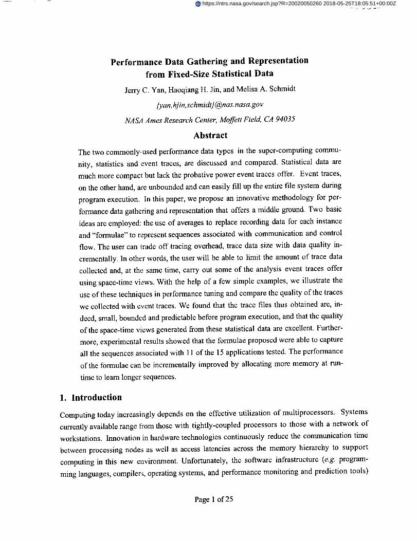
2.2 Refining Our Requirements

Based on these observations, the re-

quirements for constructing space-time

views can be stated in terms of re-

quirements to construct its three major

components: the color bars, white

spaces and message lines as summa-

rized in Table 2. For example, re-

quirement-1 in Table 2 implies that the

1. Drawing color bars:

a) identify the boundaries of all sequential code blocks

of the program (these include, procedures and

loops, if-then-else 's, and targets for goto's etc.),

b) record the duration of each code block, and

c) reconstruct the sequence in which these code blocks

occur.

2. Drawing white spaces:

a) identify all blocking constructs (e.g. sends, re-

ceives, broadcasts, barriers, waits etc.),

b) record the duration of each idling instance, and

c) record the sequence in which these white spaces oc-

cur with respect to the color bars.

3. Drawing message lines:

a) record the receiver for each send construct and the

sender for each receive construct,

b) record the ID or type for each message so thatsend's and receive's can be matched correctly I, and

c) reconstruct the sequence in which these send's andreceive's occur.

Table 2. Requirements for performance data con-

tent to construct a space-time view

control flow (for example, the branch sequence of a conditional) has to be monitored and repro-

duced in the right order. The requirements for making trace file length fixed and predictable be-

fore program execution can be formalized as shown in Table 3. It is not difficult to see how these

two sets of requirements cannot be met simultaneously. A simple example involves a program in

which process 0 sends m_ssages to ran-

domly picked processes for a random

number of times. The list of message

receivers is unboundedly long and arbi-

trary. The data required for construct-

ing a space-time view can only be

captured by an unbounded event list.

Fortunately, most real programs do not

behave in a completely random fashion.

This leaves room for the possibility of

1. The length of the trace file should be independent of

the input data (e.g. no. of iterations, problem size).

2. Trace file size may scale with the number of nodes

on which the execution takes place. We feel that the

number of storage devices could easily scale nicelywith the number of nodes.

3. Trace file size may vary with different programs but

should be independent of input data.

4. Performance data needs to be gathered for the entire

program, not limited to a portion of the execution at

the beginning.

Table 3. Defining "fixed" trace file length

For example, if node 1 sends two messages to node 2 in rapid succession; having the message ID or type will helpdetermine whether the messa_.es are received out of order.

of 25

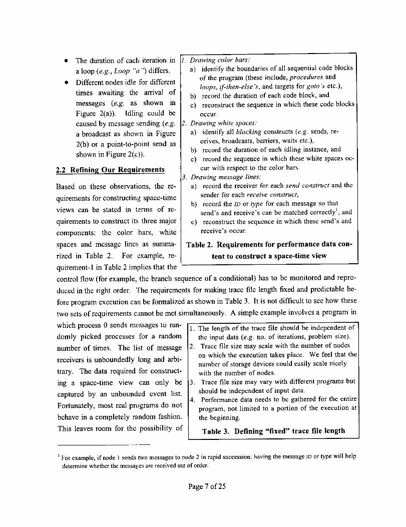
usingpatternsto captureprogrambehavior.

2.3 Collecting Data for a Space-Time View

Two basic ideas are employed to help limit the length of the trace file before program execution:

the use of"averages" to replace recording data for each instance, and "formulae" to represent in-

finitely long sequences of values. The first idea is relatively straightforward: statistical informa-

tion about total time spent in each code block and the number of times each code block 2 executes

is gathered. The space-time view constructed based on this data will only reflect "average dura-

tion" for each code block (e.g. the total time for executing a loop can be correctly represented

while it will not be possible to pinpoint exactly how long a particular iteration actually took).

a) messages node-0 ..........................

sent from node-1 _\_\\\\\N\ _ \\\_

space time node-2

diagram node-3 i\ \ \

receivers of messagesb) fromnode0 121 122123131 13213...

c) attributing message receivers according to the order

,, In in which send constructs occur in the

Isource code

s;nd-#i RI_K_I 1 1 1 1 1...!1 L_.,,n

J d-#2111 2 2 2 3 3 3..

send- #3 _1_1 2 3 1 2 3..I

-loop'-end I

Figure 3. Analyzing message patterns generated by a parallel program

The second idea is best illustrated by considering message lines on the space-time view (e.g., as

shown in Figure 3a): in order for a line to be drawn, a unique sender and a unique receiver must be

associated with each message. For all the send's along each time line to be correctly connected to

other time lines, the sequence of message receivers must be correctly reproduced (e.g., as shown

in Figure 3b). Now this seemingly complex sequence of receiver nodes originates from a sequence

of send constructs (e.g., as shown in Figure 3c (left)) that was executed. When the sequence of

receivers are broken down according to the actual source code constructs (as shown in Figure 3c

2A code block would include loops, procedures, sends/receives, as well as any "basic block" defined in the classical

sequential sense.

of 25

(right)),simplerpatternsusuallyemerge3. Thisconceptof associatingsequenceswith individualsourcecodeconstructcanactuallybeappliedto sixcategoriesof constructs:

i. thesequenceof receiversfor eachsendingconstruct,

ii. thesequenceof sendersfor eachreceivingconstruct,iii. thesequenceof messagetagsfor eachsendconstruct,

iv. thesequenceof messagetagsfor eachreceiveconstruct,v. theway inwhichbranchesaretakenatconditionalstatements,andvi. thenumberof timesaloopexecuteswhentheloopisencountered.

A methodologyfor learning the behavior of each construct as well as a suitable representation for

these patterns has to be chosen. Although there is no guarantee that any of these sequences can

be captured by a finite "formulae" (c.f behavior that are designed to be random), it remains the

subject of further experimentation as to what percentage of program constructs are, in fact, ame-

nable to this kind of analysis.

Four basic categories of formulae are proposed for learning and reproducing sequences associated

with program constructs (see Table 4):

1. IDENTITY-- repetition of one value.

2. GENERAL -- non-repeating values.

3. ITERATION -- iterative series with constant difference between individual terms.

4. CYCLE -- after some sort of prologue, the rest of the series can be represented as a repeti-

tion of a fixed number of values.

Formula Type Formula Example

Q identity an aaaaaaaaaaa

Q general a rb sc td ue v aaaabccdddde

Q iteration (a (a+i) (a+2i) ... (a+ki))n 1 3 5 7 9 1 3 5 7 9

Q cycle aPcq (a rb sc td uev) n dadbbbccddddb

Table 4. Four simple formulae used in this experiment

At run-time, the performance monitor determines whether a sequence can be captured with a

formula, and if so, which one. The user allocates a fixed amount of memory for this purpose be-

3 Program segments resemble components of a complex machinery built for a specific purpose. Although the behav-ior of the entire machine may appear complex, its components tend to exhibit relatively simple and predictable be-

havior patterns.

of 25

foreprogramexecution.Ofcourse,longerrepeatingsequencescouldbe learnedif morememorywereavailable.Nevertheless,it shouldalsobenotedthat aremanypossibleformulatypes andsomeseriescannotbecapturedbyafixed-lengthformula.

3. The AIMS Implementation

3.1 Basics of AIMS

The Automated Instrumentation and Monitoring System, or AIMS [YSM95], has been developed

at NASA Ames Research Center, under the High Performance Computing and Communications

Program. AIMS consists of a suite of software tools for measurement and analysis of parallel

program performance. An instrumentor first parses the application's source code to insert in-

strumentation at selected points. Upon execution of the instrumented program (linked with a

machine-specific monitor library), a stream of events is collected into a trace file. Runtime moni-

toring perturbs program execution and can significantly alter the recorded communication charac-

teristics and computation times. Such intrusion is removed by an intrusion-compensation

module, using appropriate communication-cost models for the underlying architecture [YL93].

The compensated trace file thus yielded can then be input to various post-processing tools that

analyze the performance characteristics of a program.

AlMS provides two post-processing tools for performance visualization: the View Kernel (VK) to

display the dynamics of program execution using a space-time view, and the Performance Index

and Statistics Kernel (Xisk) to view statistical performance data and highlight the most time con-

suming procedures and data structure interactions that may need to be tuned.

In the next few sections we proceed to discuss how AlMS is actually modified to collect statisti-

cal data, learn and record formulae for sequences, and reconstruct a space-time view for perform-

ance analysis.

3.2 Instrumentation

Instrumentation is essentially a process of source-to-source program transformation. AIMS's

instrumentor, xinstrument, first constructs a parse tree of the source code. Parse-tree nodes

that correspond to instrumentable program constructs are identified and appropriately, modified

or transformed. The instrumented source-code is then obtained by "unparsing" the transformed

parse tree. In order to gather sufficient data to reconstruct the complete dynamic behavior of the

program, xinstrument has to identify every sequential block in the program. These usually

consist of "straight-line code" between two instrumentable constructs. The example shown in

Figure 4 uses a simple conditional to illustrate how the instrumentor and the monitor cooperate

to capture control flow.

of 25

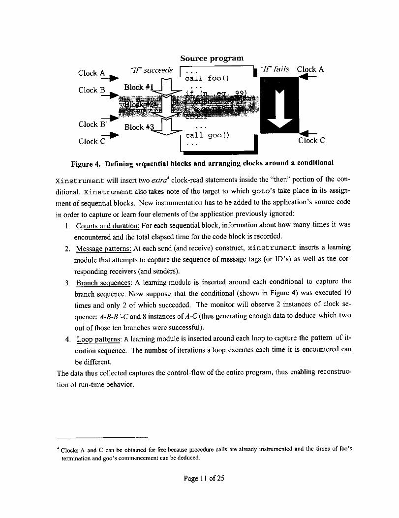
Clock A__t_ "]f" succeeds [

Clock B Block #1

Source program

Clock A

Clock B ° Block #3

Clock C Clock C

Figure 4. Defining sequential blocks and arranging clocks around a conditional

Xinstrument will insert two extra 4 clock-read statements inside the "then" portion of the con-

ditional. Xinstrument also takes note of the target to which goto's take place in its assign-

ment of sequential blocks. New instrumentation has to be added to the application's source code

in order to capture or learn four elements of the application previously ignored:

1. Counts and duration: For each sequential block, information about how many times it was

encountered and the total elapsed time for the code block is recorded.

2. Message patterns: At each send (and receive) construct, xinstrument inserts a learning

module that attempts to capture the sequence of message tags (or ID's) as well as the cor-

responding receivers (and senders).

3. Branch sequences: A learning module is inserted around each conditional to capture the

branch sequence. Now suppose that the conditional (shown in Figure 4) was executed 10

times and only 2 of which succeeded. The monitor will observe 2 instances of clock se-

quence: A-B-B '-C and 8 instances of A-C (thus generating enough data to deduce which two

out of those ten branches were successful).

4. Loop patterns: A learning module is inserted around each loop to capture the pattern of it-

eration sequence. The number of iterations a loop executes each time it is encountered can

be different.

The data thus collected captures the control-flow of the entire program, thus enabling reconstruc-

tion of run-time behavior.

4 Clocks A and C can be obtained for flee because procedure calls are already instrumented and the times of foo's

termination and goo's commencement can be deduced.

of 25

3.3 Monitoring

AIMS's performance monitoring library, the monitor, defines a set of routines that xinstru-

ment inserts into the application. They are responsible for initializing instrumentation and,

gathering and storing performance data (see [YSM95]). Because only statistical data and fixed-

length formulae are to be stored with this approach, the memory required for storing performance

data for the entire execution at each node is fixed and predictable. All performance data is written

to disk after program execution terminates.

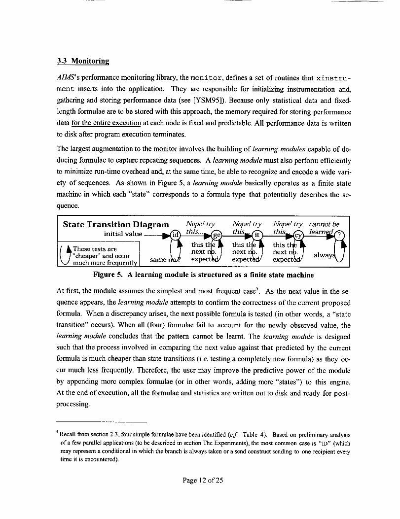
The largest augmentation to the monitor involves the building of learning modules capable of de-

ducing formulae to capture repeating sequences. A learning module must also perform efficiently

to minimize run-time overhead and, at the same time, be able to recognize and encode a wide vari-

ety of sequences. As shown in Figure 5, a learning module basically operates as a finite state

machine in which each "state" corresponds to a formula type that potentially describes the se-

quence.

State Transition Diagram Nope/ try Nope/ try Nope! try cannot be

initial valuel --_[ _These tests are ./ ] "cheaper" and occur |k./ muc_ same

Figure 5. A learning module is structured as a finite state machine

At first, the module assumes the simplest and most frequent case 5. As the next value in the se-

quence appears, the learning module attempts to confirm the correctness of the current proposed

formula. When a discrepancy arises, the next possible formula is tested (in other words, a "state

transition" occurs). When all (four) formulae fail to account for the newly observed value, the

learning module concludes that the pattern cannot be learnt. The learning module is designed

such that the process involved in comparing the next value against that predicted by the current

formula is much cheaper than state transitions (i.e. testing a completely new formula) as they oc-

cur much less frequently. Therefore, the user may improve the predictive power of the module

by appending more complex formulae (or in other words, adding more "states") to this engine.

At the end of execution, all the formulae and statistics are written out to disk and ready for post-

processing.

Recall from section 2.3, four simple formulae have been identified (c.f Table 4). Based on preliminary analysis

of a few parallel applications (to be described in section The Experiments), the most common case is "lD" (whichmay represent a conditional in which the branch is always taken or a send construct sending to one recipient everytime it is encountered).

of 25

3.4 Post-processing (Event Trace Reconstruction)

In order to construct a space-time view from the performance data (in the form of statistics and

formulae) gathered using this approach, time-ordered events need to be generated. A simple algo-

rithm has been implemented to accomplish this process:

/ _xeluYed _ send to nodes 1 to ,.

/;4Proc : A_ 8 times I ..... I 8 in sequence,...) [PatternH

2_ b _kmed'_ _anch_ _'iV_l al°vdaY0s;et_i_!t°g20 g

"N. taken _[ node 0) _/..... I duration: average... ---"" lseq. cocte. I m-_.., min.., first: ... ""

Figure 6. Annotated source tree ready for event-trace reconstruction

1. BUILD PARSE TREE based on lexical information about the source code collected by xin-

s t rument.

2. ANNOTATE PARSE TREE using performance data. As shown in Figure 6, the annotation

process involves the association of performance statistics and formulae to instrumented

constructs and sequential code blocks. These associations allow the reconstruction of

elapsed times, branch sequences, iteration counts, and message receiver/sender/tag se-

quences in the next two steps.

3. RECONSTRUCT CONTROL FLOW via annotated parse tree traversal. Program execution is

simulated as the parse tree is traversed node-by-node in lexical order. At specific points

where control flow information was determined dynamically, e.g. the way a branch took or

the number of times a loop executed, the stored formulae associated at that node is used

(c.f at points c and d of Figure 6).

4. GENERATE INTERVAL DURATION at each node. The amount of time spent at each node can

be approximated by the statistical performance data associated at each parse-tree node.

5. CHECK CONSISTENCY OF EVENT TIMES ACROSS NODES when communication occurs. This

process of ensuring messages are sent before they are received also facilitates periodical

cross-checking and adjustment of elapsed times at each processing node, thus resulting in a

more consistent picture of the entire execution (cf. with Figure 6, at point f for processing

node 0 and point g tor other nodes).

6. GENERATE TIMED EVENTS. The events are then collected as a time-ordered trace file for VK

to build a space-time view.

of 25

4. The Experiments

4.1 Quality of Statistical Space-time Diagram

The methodology described here was applied to a few test programs and the NAS parallel

benchmarks (NPB) [BB*91]. To illustrate the quality of the space-time diagram generated from

statistical data, three examples, matraul (Figure 7) and the NAS parallel benchmarks SP (Figure

8) and BT (Figure 9), were compared with actual event traces. It can be seen that the overall

characteristics of event traces is correctly represented by the space-time view derived from sta-

tistics: 1) the control flow of program executions was correctly recorded, 2) critical points (such

as message passing, global blocking) were illustrated, 3) the total execution time was very close.

The exception of the durations of individual iterations of a loop in matmul (c.f. Figure 2) is due

to that averaged durations were used in the construction of the space-time views from statistics.

- [i

t_-w- nu- ;..

1

t;iii

I!

........Figure 7. Space-time view for matmuh from a) event traces, and b) statistics gathered

The total execution times of the six tested applications are summarized in Table 5. For a com-

parison, the corresponding values for uninstrumented and instrumented (i.e. event traces) are also

included in the table. These values were taken from averages of three repeated runs for each ap-

plication on 4 nodes of an IBM SP2. The overhead due to the instrumentation is reflected by 5

to 10% increase of execution time for the instrumented codes. The execution times for the two

types of instrumentations (to produce event traces and statistical data) are very close. The

slightly longer time (< 5%) to produce statistical traces is due to the extra cost of instrumenting

control constructs, such as IF and LOOP statements, and the current implementation of the

learning module.

of 25

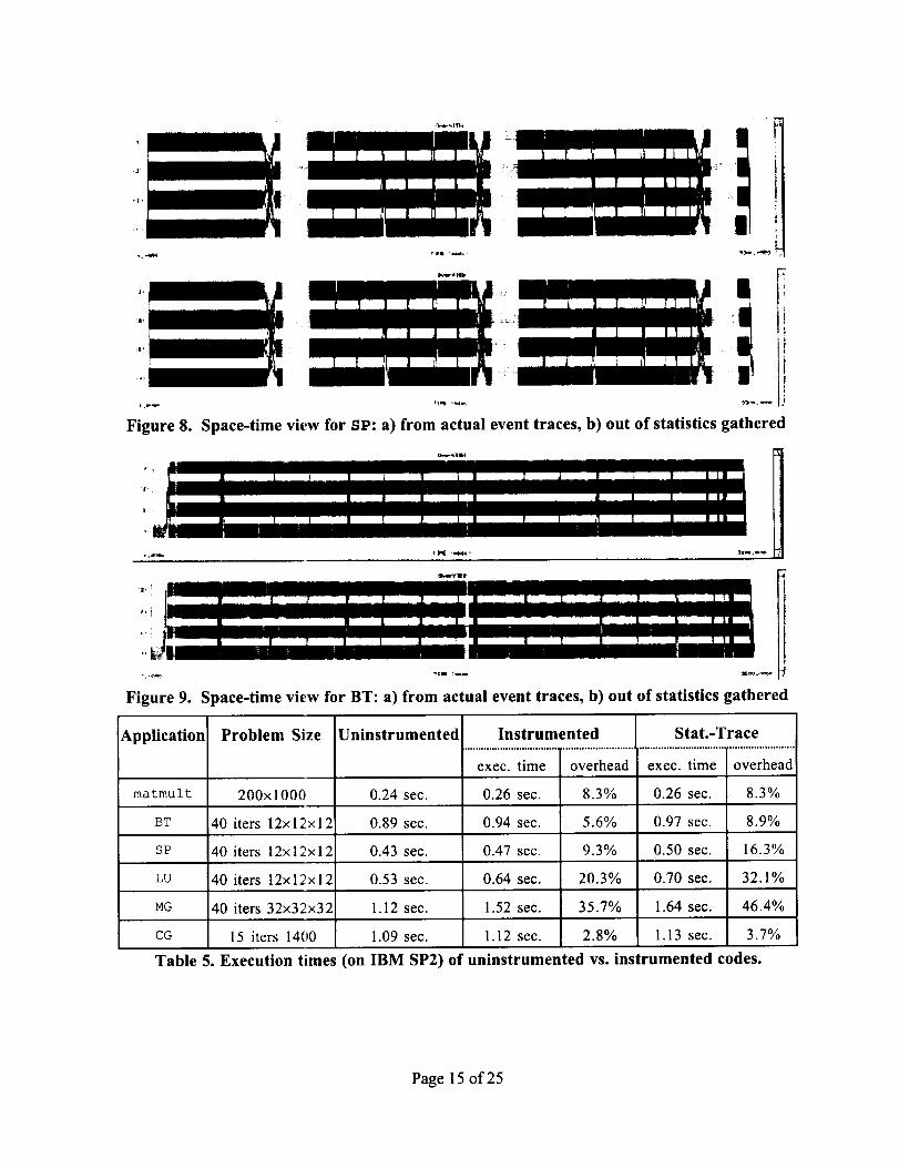
Figure 8. Space-time view for SP: a) from actual event traces, b) out of statistics gathered

ct..._llt_ 1

Figure 9. S

Application

race-time view for BT: a) from actual event traces, b) out of statistics gathered

Problem Size Uninstrumented Instrumented Stat.-Trace

...... .......matmult 200x1000 0.24 sec. 0.26 sec.

BT 40 iters 12x12x12 0.89 sec. 0.94 sec.

sP 40 iters 12x12x12 0.43 sec. 0.47 sec.

LU

8.3% 0.26 sec. 8.3%

5.6% 0.97 sec. 8.9%

9.3% 0.50 sec. 16.3%

40 iters 12x12×12 0.53 sec. 0.64 sec. 20.3% 0.70 sec. 32.1%

MG 40 iters 32x32x32 1.12 sec. 1.52 sec. 35.7% 1.64 sec. 46.4%

CG 15 iters 1400 1.09 sec. 1.12 sec. 2.8% 1.13 sec. 3.7%

Table 5. Execution times (on IBM SP2) of uninstrumented vs. instrumented codes.

of 25

4.2 Detailed Comparison of Trace Files

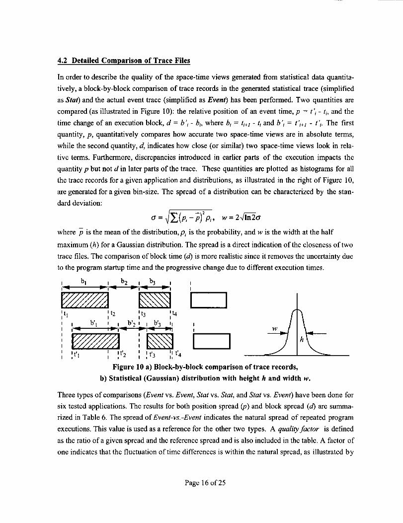
In order to describe the quality of the space-time views generated from statistical data quantita-

tively, a block-by-block comparison of trace records in the generated statistical trace (simplified

as Star) and the actual event trace (simplified as Event) has been performed. Two quantities are

compared (as illustrated in Figure 10): the relative position of an event time, p = t'i - ti, and the

time change of an execution block, d = b '_- b;, where bi = t;+l - t_and b '_ = t',l - t';. The first

quantity, p, quantitatively compares how accurate two space-time views are in absolute terms,

while the second quantity, d, indicates how close (or similar) two space-time views look in rela-

tive terms. Furthermore, discrepancies introduced in earlier parts of the execution impacts the

quantity p but not d in later parts of the trace. These quantities are plotted as histograms for all

the trace records for a given application and distributions, as illustrated in the right of Figure 10,

are generated for a given bin-size. The spread of a distribution can be characterized by the stan-

dard deviation:

or= p_-p p_, w=2 i_-_-0"

where p is the mean of the distribution, p_ is the probability, and w is the width at the half

maximum (h) for a Gaussian distribution. The spread is a direct indication of the closeness of two

trace files. The comparison of block time (d) is more realistic since it removes the uncertainty due

to the program startup time and the progressive change due to different execution times.

J bi i b2 i 1°3 t ii_ ""- I -"' t"'- I -"_ _1 I

tlt2 It 3 tit4

i b' 1 i i b' 2 t i b' I I. _ _ 3 _ II TM ' ""- I TM "Y l -" "11 I

I t'l I it, 2 I I III , I , t'3 I, t'4

Figure 10

5) Statistical

tl

Three types of comparisons

a) Block-by-block comparison of trace records,

(Gaussian) distribution with height h and width w.

(Event vs. Event, Star vs. Star, and Stat vs. Event) have been done for

six tested applications. The results for both position spread (p) and block spread (d) are summa-

rized in Table 6. The spread of Event-vs.-Event indicates the natural spread of repeated program

executions. This value is used as a reference for the other two types. A quality factor is defined

as the ratio of a given spread and the reference spread and is also included in the table. A factor of

one indicates that the fluctuation of time differences is within the natural spread, as illustrated by

of 25

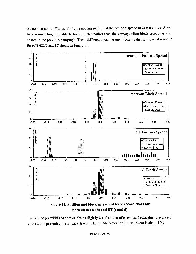
thecomparisonof Stat vs. Stat. It is not surprising that the position spread of Stat trace vs. Event

trace is much larger (quali_ factor is much smaller) than the corresponding block spread, as dis-

cussed in the previous paragraph. These differences can be seen from the distributions ofp and d

for MATlVlUr,T and BT shown in Figure I 1.

0.8

0.6

0.4

0.2

0

-0.05

L","r-,.,O

oa.,

0.8

N

0.6

o0.4

0.2

0

-0.20

0.6

I i:

-0.04 43.03 -0.02 43.01 0 0.0! 0.02

-0.16 -0.12 -0.08 43.04 0.00 0.04

k

0.03 0,04

matmult Position Spread

liSt.at vs. Event [

,_Event vs. Event I, Stat vs. Stat I

I I

0.05 0.06 0.07 0.08

matmult Block Spread

liStatvs. Event [

,> Event vs. Event I

,+Stat vs. Stat [

0.08 0.12 0.16 0.20

0,4

0.2

0

43.05

0.6

¢0e_

-0.04 -0.03 -0.02 -0.01 0 0.01 0.02

BT Position Spread

urnSlat vs. Event I

.X Event vs. Event[

._ Stat vs. Stat ]

. _.nnn.,. nnIn,n.lnn.0._ 0.04 0.05 0.05 0._ 0.08

0.4

0.2

-r-,

.on..,

BT Block Spread

, ..... _ _. _.-0.12 -0.08 -0.134 0.00 0.04 0.138 0,12 0.16

nStat vs. Event [

Event vs. Event

>: Stat vs. Stat

0

-0.2O -0.16 0.20

Figure 11. Position and block spreads of trace record times for

matmult (a and b) and BT (c and d).

The spread (or width) of Stat vs. Stat is slightly less than that of Event vs. Event: due to averaged

information presented in statistical traces. The quality factor for Stat vs. Event is about 10%

of 25

worse(fromtheblockspread)thanthatforEvent vs. Event. This is a reflection of the use of av-

eraged execution times for program constructs in the process of reconstructing the space-time

view. This averaged representation would be distinguished in a real event trace, for example, exe-

cution time of a function call would be different with different input parameters, which could not

be represented in the statistical trace.

Position Spread (w) Block Spread (w)

Application Eventvs. Stat vs. Stal Stat vs. Eventvs. Stat vs. Stat Stat vs.

Event Event Event Event

matmult 3.36 3.38 (0.99) 3.50 (0.96) 0.037 0.033 (1.11) 0.039 (0.95)

BT 3.48 3.36 (1.04) 15.1 (0.23) 0.039 0.038 (1.04) 0.047 (0.83)

SP 3.31 3.32 (1.00) 11.3 (0.29) 0.039 0.037 (1.06) 0.048 (0.81)

LU 3.29 3.29 (1.00) 5.00 (0.66) 0.035 0.034 (1.01) 0.037 (0.93)

MG 3.29 3.29 (1.00) 12.3 (0.27) 0.035 0.034 (1.03) 0.040 (0.87)

CG 3.56 3.86 (0.92) 5.50 (0.65) 0.042 0.033 (1.27) 0.044 (0.95)

Table 6. Spreads of relative position and block time from different program executions

(on IBM SP2, in milliseconds). The quality factors (see text) are enclosed in parenthesis.

4.3 Trace File Size

Experiments have also been performed on trace file sizes. Figure 12 compares the variation of

trace file size when SP and BT are executed with a problem size of 12x12x12. It is not surprising

that the size of event trace files increases linearly as the problem size goes larger, while the size

of statistical files remains constant. Based on this data, we can easily project that for full-scale

executions (with problem size 162x 162x 162 for 200-400 iterations) it will be very difficult to use

event tracing to obtain performance data. More experiments on various parallel programs (such

as other NAS Parallel Benchmarks) are performed and similar results are obtained since the pro-

posed methodology is designed to produce a small fixed length trace file.

As can be seen from the next section, the use of fixed length formulae in the statistical tracing en-

ables us to capture more than 90% of the execution sequences, and with the increase of formula

size this percentage also increases, yielding always predictable trace file size. For those truly

random execution sequences, multiple or variable-length formulae may be used although the size

of the resulted trace file may increase. However, since random execution sequences usually are

very small percentage (less than a few percent) of the whole program execution, the change of the

trace file size is expected to be nominal (less than a few percent of the increase in a real event

trace file).

of 25

1400

1200

._ 1000800

6oo400

[-200

0

30000d.

"SP" on 4 Nodq _ 25000

/ i _ 213000

ra)O-'- Event Trace

- -_- Extended Statistics

m.B. 'J"

No. of Iteratio_q P I

25 50 75 1000

N15000

i0000

50o0

0

"BT" on 4 Nod_

Jf

I --XmEvent Trace- .a- Extended Statistics I

fNo. of Iteration

D- -m- - - 4- - -m-- - _

0 5 10 15 20

Figure 12. Trace file size comparison

In summary, the space-time view derived from the statistical data (stat-trace) gives a reasonable

representation of the overall trace picture with critical points accurately demonstrated (important

for performance analysis). The use of stat-tracing eliminates the need of trace flushing in the mid-

die of program execution and,

thus, produces trace file with less

distortion and predictable size.

When problem size gels very

large, event trace becomt;s very

large and statistical trace wins.

4.4 Ability. to Capture Applica-

tion Characteristics

Perhaps many readers are won-

dering how effective these four

formulae were in capturing se-

quences associated with parallel

applications. Figure 13 puts the

applications tested along two

axes. The y-axis, labeled "No. of

Individual Send/Recv Con-

structs", measures the (static)

complexity of the source code.

The x-axis, labeled "No. of mes-

sages Sent", measure s the

900

800

700

600

500

400

3O0

200

100

t_

o

o

o

o

6ZI mpibtl6

Impispl6 860arc2d16

ll pvmmg32

la m2-64

pvmmg l 6

_ m2-32

I_ mpimg16

lm2-16

| pvmtransl6

] pvmmert5

0 2oooo

[] 860arc2d32

ApplicationCommunicationCharacteristics

I mplcgl6

mptlu 16I

pvmcg l 7I

No. of Messages Sent

40000 6(KI30 80000 100000

Figure 13. Characteristics of applications tested

of 25

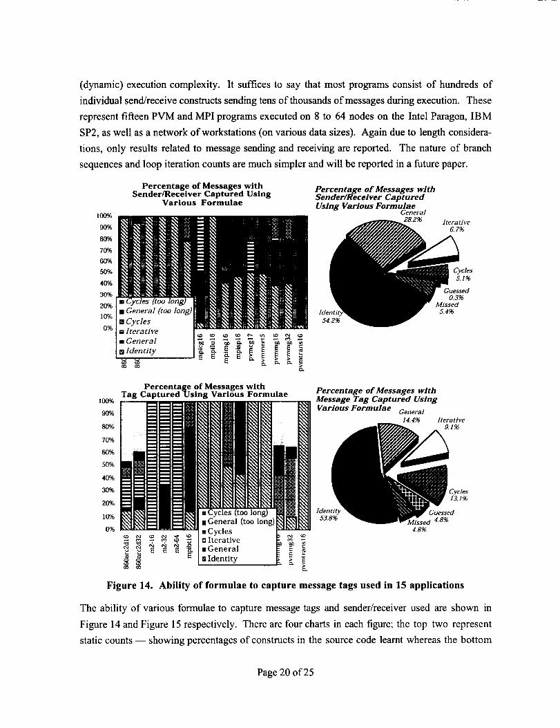
(dynamic)executioncomplexity. It sufficesto say that most programs consist of hundreds of

individual send/receive constructs sending tens of thousands of messages during execution. These

represent fifteen PVM and MPI programs executed on 8 to 64 nodes on the Intel Paragon, IBM

SP2, as well as a network of workstations (on various data sizes). Again due to length considera-

tions, only results related to message sending and receiving are reported. The nature of branch

sequences and loop iteration counts are much simpler and will be reported in a future paper.

10096

90%

8O%

7O%

6O%

5O%

4O%

30%

2O%

10%

0%

Percentage of Messages with

Sender/Recelver Captured UsingVarious Formulae

BItera tire

Percentage of Messages wtthSender�Receiver Captured

Using Various FormulaeGeneral

28.2%

54.2%

Iterative

6. 7%

Cycles£1%

Guessed0,3%

Missed£4%

Percentage of Messages withTag Captured Using Various Formulae

1oo%

90% Various Formulae

8o%

70%

°,50%

40%

30%

20%

I o_ _ _ _ _E_lBidentity _- i _ Iden_

10% 53.8%

0%

¢xl t'_ t'Xl .0"_ _n eG nerai F -E' ._

• E _"

e_

Percentage of Messages wtth

Message Tag Captured Using

General

14.4% Iterative9.1%

Cycles13.1%

_uessed4.8%

4.8%

Figure 14. Ability of formulae to capture message tags used in 15 applications

The ability of various formulae to capture message tags and sender/receiver used are shown in

Figure 14 and Figure 15 respectively. There are four charts in each figure; the top two represent

static counts -- showing percentages of constructs in the source code learnt whereas the bottom

of 25

two representdynamiccounts-- showingpercentagesof messagesactuallysentduringexecu-tion. Thepie chartson theright representsummariesof thedetaileddatadisplayedon theleft.

100%

90%

80%

70%

60%

50%

40%

30%

20%

10%

0%

_D

O

Percentage of Constructs withSender�Receiver Captured Using

Various Formulae

_Cyclesn Itera tire

• General

mldentity¢).

Percentage of Constructs with

Sender�Receiver Captured

Using Various Formulae

General23.6%

ldentity71.3%

lteratlve

2. 7%

Cycles1.2%

Missed

1.3%

Percentage of Constructs with Message

Tag Captured Using Various Formulae

100%

90%

8O%

70%

60%

5O%

4096

30%

20%

10%

0%

_o oo

Figure 15.

n [terattve

• General

D Identity

Percentage of Constructs with

Message Tag Captured UsingVarious Formulae

General16. 7%

Identity65. 7%

IterativeZl%

Cycles4.8%

Missed5.8%

Ability of formulae to capture senders/receivers used in 15 applications

A number of observations can be made. First, the formulae capture all message tags in 11 test

cases and all sender/receiw:rs in 13 of the 15 test cases 6. Second, the "[D" formula accounts for

most cases: in other words, most programmers use a constant in their code for message tag and

6 The reader should note that the percentage of sequences learnt depends on the length of formulae. The data pre-

sented here represent formulae of a maximum sequence length of 18. Longer sequences can be learnt by allocatingmore memory for monitoring at run-time.

of 25

sender/receiver.Finally the reconstruc-tion algorithmcanactuallyobtainsomeof thenumbersin the sequencesup to

thepointwheretheformulafailed.

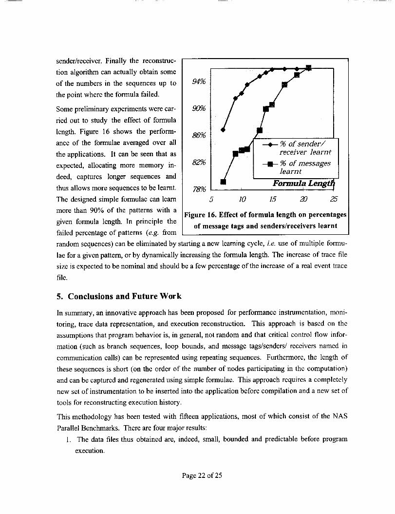
Somepreliminaryexperimentswerecar-

fled out to study the effectof formulalength.Figure 16 showsthe perform-anceof the formulaeaveragedover all

theapplications.It canbeseenthat asexpected,allocatingmore memory in-deed, captureslongersequencesand

thusallowsmoresequencestobe learnt.Thedesignedsimpleformulaecanlearnmorethan90% of the patternswith a

givenformulalength.In principle the

94%

9O%

86%

82%

78%

m

1 1 q

5 10 15 20 25

Figure 16. Effect of formula length on percentages

of message tags and senders/receivers learntfailed percentage of patterns (e.g. from

random sequences) can be eliminated by starting a new learning cycle, i.e. use of multiple formu-

lae for a given pattern, or by dynamically increasing the formula length. The increase of trace file

size is expected to be nominal and should be a few percentage of the increase of a real event trace

file.

5. Conclusions and Future Work

In summary, an innovative approach has been proposed for performance instrumentation, moni-

toring, trace data representation, and execution reconstruction. This approach is based on the

assumptions that program behavior is, in general, not random and that critical control flow infor-

mation (such as branch sequences, loop bounds, and message tags/senders/receivers named in

communication calls) can be represented using repeating sequences. Furthermore, the length of

these sequences is short (on the order of the number of nodes participating in the computation)

and can be captured and regenerated using simple formulae. This approach requires a completely

new set of instrumentation to be inserted into the application before compilation and a new set of

tools for reconstructing execution history.

This methodology has been tested with fifteen applications, most of which consist of the NAS

Parallel Benchmarks. There are four major results:

1. The data files thus obtained are, indeed, small, bounded and predictable before program

execution.

of 25

2. Thequalityof thespace-timeviewsgeneratedfromthesestatisticaldataisexcellent.3. Experimentalresultsshowthattheformulaeproposedwereableto capture95%of these-

quencesinvolvingmessagesendingandreceiving(themostcomplicatedamongthe sixcate-goriesmentionedin section4.4). Thiscorrespondsto 100%of all thesequencesassociatedwith 11of the 15applications.

4. Theperformanceof theformulaecanbe incrementallyimprovedby allocatingmoremem-oryatrun-timeto learnlongersequences.

By theuseof variable-lengthformulaeormultipleformulae,executionsequencescanbelearnt100%.However,theimpactonthetracefile sizeneedsfurtherinvestigation.Moreexperiments

areneededto studytheintrusionof thelearningmoduleandextrainstrumentationoncontrolflows,whichmaypinpointto futureimprovementsof ourimplementation.In particular,work

still needsto beperformedin two majorareasto fully evaluatetheapplicabilityof thisapproachfor actualsystems:Dealing with unknowns -- Sequences that are either very long or truly non-repeating (e.g. as a

result of non-determinism) cannot be learned. Even though experimental results suggest that these

comprise less than 5% of lhe sequences associated with the programs we tested, they pose po-

tential problems for event trace reconstruction. Message lines cannot be drawn on the space-time

diagram when sequences associated message transmission cannot be reconstructed. Failure to re-

construct sequences associated with control-flow is much more problematic; the "remedy" de-

pends on the type, past behavior and the context in the particular control-flow construct occur.

In some cases, these potentially problematic constructs can be identified at instrumentation time

and the user can be alerted to provide alternatives. Otherwise, the monitor can decide to fall-back

on event-tracing for this small percentage of construct, still resulting in a much smaller trace file

than a "pure event trace".

Characterizing and reducing run-time overhead -- Although the most intrusive element for event

tracing (namely the need to flush trace records to disk) has been eliminated, more constructs are

instrumented and the cost of executing complex learning modules could become expensive. Nev-

ertheless, with the current formulations and test cases, this mode of monitoring exerts less over-

head than event tracing.

6. References

[Pan91] C. M. Pancake, "Software Support for Parallel Computing: Where Are We Headed?"

Communications oftheACM, Vol. 34, No. 11, 1991, pp. 52-64.

of 25

[SMS95]T. Sterling,P. Messina and P. H. Smith, Enabling Technologies for Petaflops Com-

puting, MIT Press, 1995 (see URL http://www-mitpress.mit.edu/mitp/recentbooks/

comp/enabling-petaflops.html).

[Hea93] M. T. Heath, "Recent Developments and Case Studies in Performance Visualization

using ParaGraph," in Performance Measurement and Visualization of Parallel Systems,

ed. G. Hating and G. Kotsis, Elsevier Science, 1993, pp. 175-200.

[Mi193] Bart Miller. "What to Draw? When to Draw? An Essay on Parallel Program Visualiza-

tion", Journal of Parallel and Distributed Computing, Vol. 18, No. 2 (June 1993).

[YSM95] J. C. Yan, S. R. Sarukkai, and P. Mehra. "Performance Measurement, Visualization

and Modeling of Parallel and Distributed Programs using the AIMS Toolkit". Software

Practice & Experience. April 1995. Vol. 25, No. 4, pages 429-461

[RO*91] D. A. Reed, R. D. Olson, R. A. Aydt, T. M. Madhyastha, T. Birkett, D. W. Jensen, B.

A. A. Nazief, and B. K. Totty. "Scalable Performance Environments for Parallel Sys-

tems." In Proceedings of the 6th Distributed Memory Computing Conference. April

1991.

[HIM91] J. Hollingsworth, R. Irvin, and B. Miller, "The Integration of Application and System

Based Metrics in a Parallel Program Performance Tool," Proc. ThirdACMSIGPLAN

Symp. on Principles and Practice of Parallel Programming (PPOPP), pp. 189-200,

1991.

[HE91 ] M. Heath and J. Ethtidge. "Visualizing the Performance of Parallel Programs." IEEE

Software, Vol. 8, No. 5, Sept. 1991, pp. 29-39.

[MC'95] Barton P. Miller, Mark D. Callaghan, Jonathan M. Cargille, Jeffrey K. Hollingsworth

R. Bruce Irvin, Karen L. Karavanic, Krishna Kunchithapadam, and Tia Newhall. IEEE

Computer 28, 11 (November 1995). Special Issue on Performance Evaluation Tools for

Parallel and Distributed Computer Systems.

[SYG94] S. R. Sarukkai J. Yan and J. K. Gotwals, "Normalized Performance Indices For Mes-

sage Passing Parallel Programs," Proc. of International Conference on Supercomputing,

Manchester, England, July 1994.

[SK90] Performance Instrumentation and Visualization. M. Simmons, R. Koskela Ed., ACM

Press. 1990.

[YL93] J.C. Yan and S. Listgarten. "Intrusion Compensation for Performance Evaluation of

Parallel Programs on a Multicomputer". Proceedings of the ISCA 6th International Con-

ference on Parallel and Distributed Computing Systems, Louisville, KY, October 14-16,

1993, pages 427-431.

of 25

[GL*92]D.Gannon,J.K. I,ee,B. Shei,S.R.Sarukkai,etal.,"SigmalI:A toolkit forBuilding

ParallelizingCompilersandPerformanceAnalysisSystems,"Proc.Programming Envi-

ronments for Parallel Computing Conf. Edinburgh, April 1992.

[PMY95] Special Issue on Performance Evaluation Tools for Parallel and Distributed Systems,

Ed., Cherri M. Pancake, Margaret L. Simmons, and Jerry C. Yan. IEEE Computer, No-

vember 1995, Vol. 28, No. 11.

[BB*91]D. Bailey, J. Barton, T. Lasinski, and H. Simon (eds.), "The NAS Parallel Benchmarks,"

Report RNR-91-002, NASA Ames Research Center, January 1991.

of 25

?r=20020050260 2018-02 · pdf file · 2013-08-30performance data gathering and...

Documents