1

HYDROLOGICAL MODELLING IN THE LUVUVHU CATCHMENT Jewitt, G.P.1 and Garratt, J.A.2

(ZF0150/R7937 – DFID/FRP)

1School of Bioresources Engineering and Environmental Hydrology, University of KwaZulu-Natal, South Africa 2Centre for Land Use and Water Resources Research, University of Newcastle, Newcastle upon Tyne, UK.

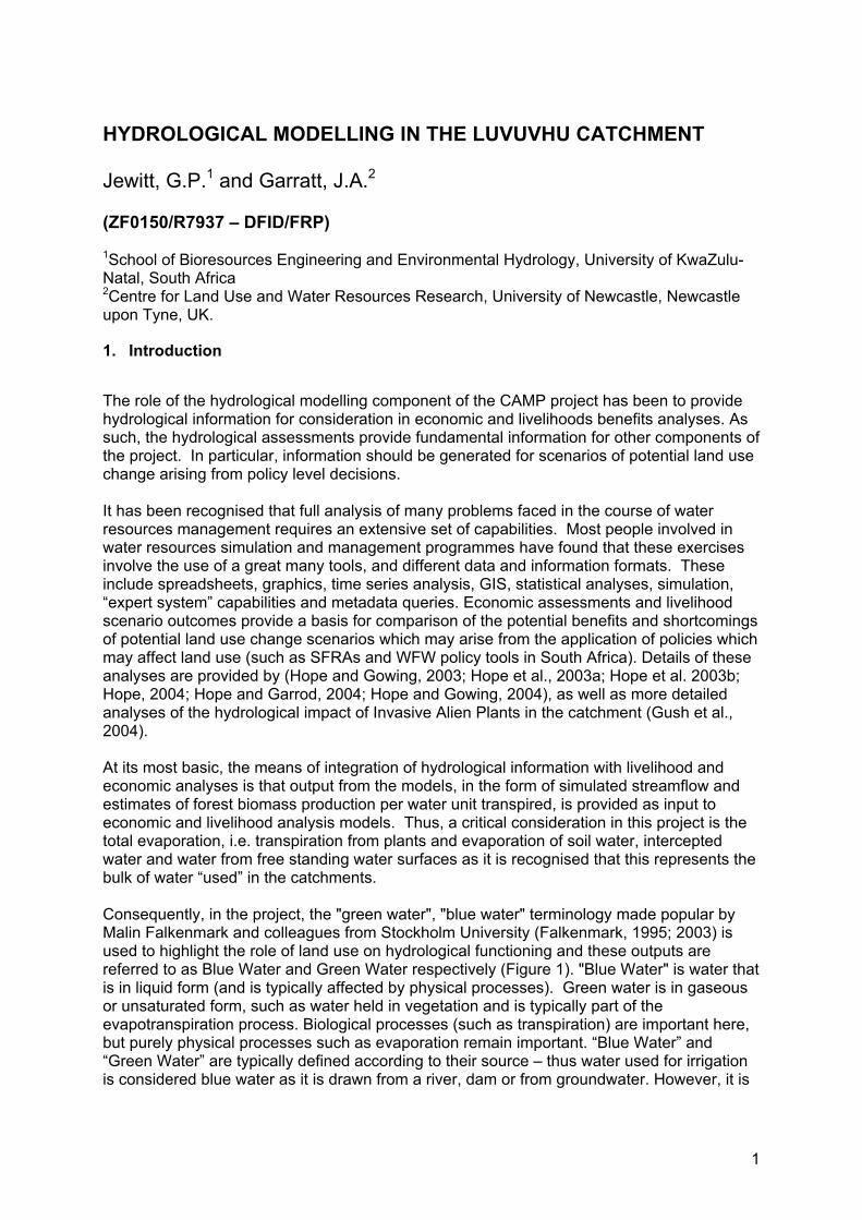
1. Introduction The role of the hydrological modelling component of the CAMP project has been to provide hydrological information for consideration in economic and livelihoods benefits analyses. As such, the hydrological assessments provide fundamental information for other components of the project. In particular, information should be generated for scenarios of potential land use change arising from policy level decisions. It has been recognised that full analysis of many problems faced in the course of water resources management requires an extensive set of capabilities. Most people involved in water resources simulation and management programmes have found that these exercises involve the use of a great many tools, and different data and information formats. These include spreadsheets, graphics, time series analysis, GIS, statistical analyses, simulation, “expert system” capabilities and metadata queries. Economic assessments and livelihood scenario outcomes provide a basis for comparison of the potential benefits and shortcomings of potential land use change scenarios which may arise from the application of policies which may affect land use (such as SFRAs and WFW policy tools in South Africa). Details of these analyses are provided by (Hope and Gowing, 2003; Hope et al., 2003a; Hope et al. 2003b; Hope, 2004; Hope and Garrod, 2004; Hope and Gowing, 2004), as well as more detailed analyses of the hydrological impact of Invasive Alien Plants in the catchment (Gush et al., 2004). At its most basic, the means of integration of hydrological information with livelihood and economic analyses is that output from the models, in the form of simulated streamflow and estimates of forest biomass production per water unit transpired, is provided as input to economic and livelihood analysis models. Thus, a critical consideration in this project is the total evaporation, i.e. transpiration from plants and evaporation of soil water, intercepted water and water from free standing water surfaces as it is recognised that this represents the bulk of water “used” in the catchments. Consequently, in the project, the "green water", "blue water" terminology made popular by Malin Falkenmark and colleagues from Stockholm University (Falkenmark, 1995; 2003) is used to highlight the role of land use on hydrological functioning and these outputs are referred to as Blue Water and Green Water respectively (Figure 1). "Blue Water" is water that is in liquid form (and is typically affected by physical processes). Green water is in gaseous or unsaturated form, such as water held in vegetation and is typically part of the evapotranspiration process. Biological processes (such as transpiration) are important here, but purely physical processes such as evaporation remain important. “Blue Water” and “Green Water” are typically defined according to their source – thus water used for irrigation is considered blue water as it is drawn from a river, dam or from groundwater. However, it is

2

recognised and accepted that irrigation provides a means of meeting green water needs to be redirecting blue water to green (Rockstrom, pers. Comm.).

Figure 1 Green and Blue Water flows and the role of land use.

2. Model Requirements

From a hydrological modelling perspective, any model considered for use in projects which adopt the CAMP approach must be able to simulate runoff (blue water) and total evaporation (green water) at an appropriate spatial and temporal scale for different land uses. In particular, it is the sensitivity and ability to accurately simulate changes in catchment land use that are fundamental to this project.

2.1 Spatial and temporal scale

It has been said, that a "good" model does not attempt to reproduce every detail of the biophysical system. Rather, the objective of the model should be to see how much detail can be “ignored” without producing results that contradict available observations at particular scales of interest (Levin, 1992). However, no single model of catchment processes will adequately explain observed patterns at all scales. Models operate at their own unique and often disparate scales, and in order to explain patterns at other scales, other models are needed. The question of appropriate scale for analyses is a problematic one, particularly in interdisciplinary studies. In this study, the modelling approach has considered both detailed spatial modelling of the Luvuvhu Catchment at daily time scales (ACRU – Appendix I), as well coarser spatial representation through hydrological modelling at the quaternary catchment scale at a daily time step (HYLUC – Appendix II). Whilst most livelihood and economic analyses rely on input information at quaternary catchment scale at monthly or annual time-steps, the benefit of the more detailed hydrological modelling approach is that output from these models are easily

3

aggregated to these levels. Furthermore, in some cases analyses at a range of temporal scales are required. For example, whilst livelihood links to green water use are analysed annually, assessment of whether the Basic Human Needs Water Requirements (BHNR) requires analyses of daily flow (Hope et al., 2003b).

2.2 Hydrological Modelling in the Luvuvhu Catchment

Two landuse sensitive hydrological models, HYLUC (Calder, 2003) and the ACRU Agrohydrological modelling system (Schulze, 1995), both of which have been used extensively in forestry related studies (Calder, 1999; Jewitt and Schulze, 1998) have been configured for use in the Luvuvhu. The configuration of the ACRU model is described in detail in Appendix I, and the configuration of HYLUC is described in Appendix 2.

3 The Luvuvhu Catchment – Important Characteristics

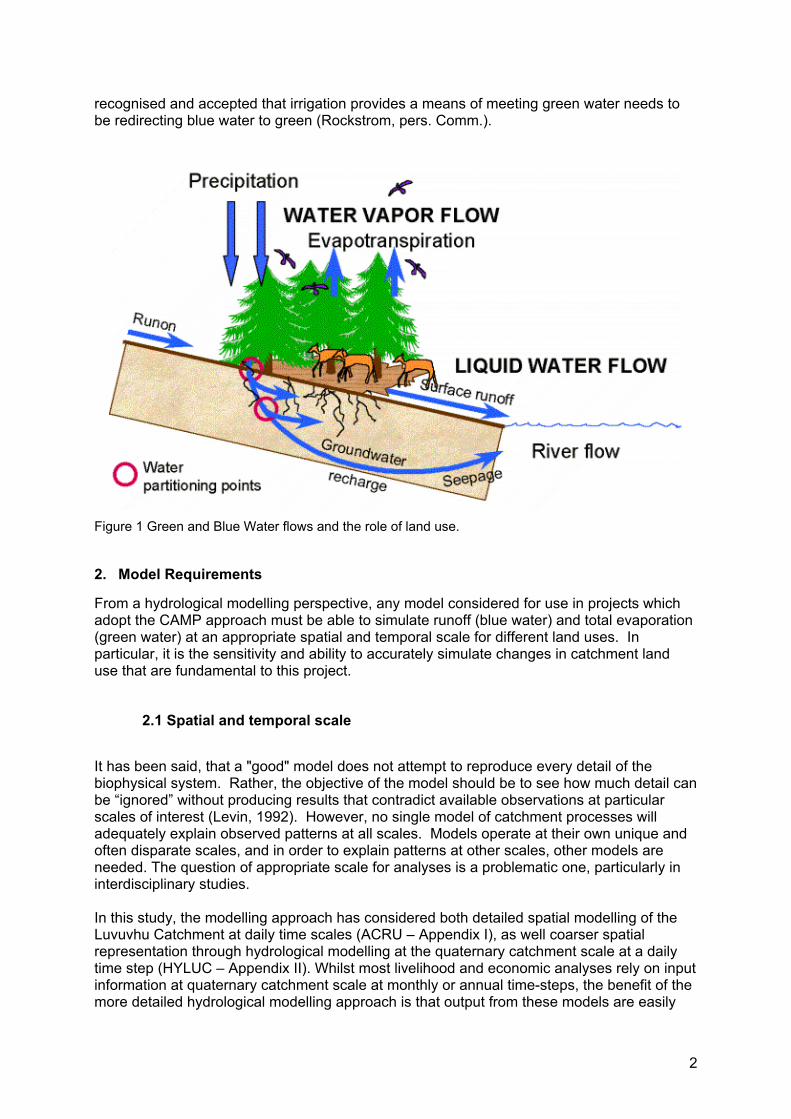
The Luvuvhu Catchment is found in the Limpopo Province, South Africa and together with the Letaba Catchment forms the Luvuvhu/Letaba Water Management Area (WMA), one of 18 WMAs (Figure 2) identified by the South African Department of Water Affairs and Forestry (DWAF). The Luvuvhu Catchment forms part of the larger Limpopo system which drains into the sea in northern Mozambique.

MOZAMBIQUE

CapeTown

Port Elizabeth

East London

Durban

Pretoria

Johannesburg

Bloemfontein

BOTSWANA

ZIMBABWE

NAMIBIA

WATER MANAGEMENT AREAS

3. Crocodile (West) and Marico

1. Limpopo

4. Olifants

6. Usutu to Mhlatuze

7. Thukela

8. Upper Vaal9. Middle

Vaal

10. Lower Vaal

12. Mzimvubu to Keiskamma

13. Upper Orange

15. Fish to Tsitsikamma

16. Gouritz18. Breede

19.Berg

17.Olifants/Doorn

14. Lower Orange

ProvincialBoundaries

Water ManagementArea Boundaries

11. Mvoti to Umzimkulu

2. Luvuvhuand Letaba

5. Inkomati

Figure 2 Water Management areas of South Africa (DWAF, 2002)

The Luvuvhu River drains an area of 5 941 km2. The catchment has been subdivided into 14 DWAF quaternary catchments (Figure 3). Mean Annual Precipitation (MAP) over the Luvuvhu catchment is 608 mm, mean total evaporation is 1 678 mm and natural MAR is

4

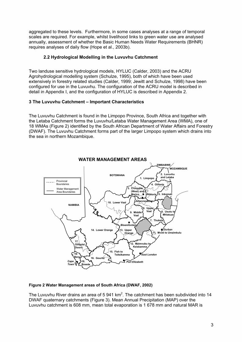
estimated to be 520 x106 m3. However, all of these show high spatial and temporal variation (Figure 3) with highest rainfall and lowest ET over the Soutpansberg mountain range in the west and the lowest rainfall and highest potential ET in the arid areas in the west of the catchment adjacent to the Kruger National Park.

Figure 3 Quaternary catchments and water transfers of the Levuvu/Letaba Water Management Area.

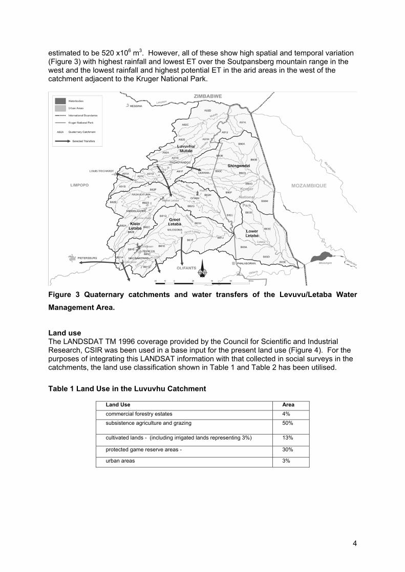
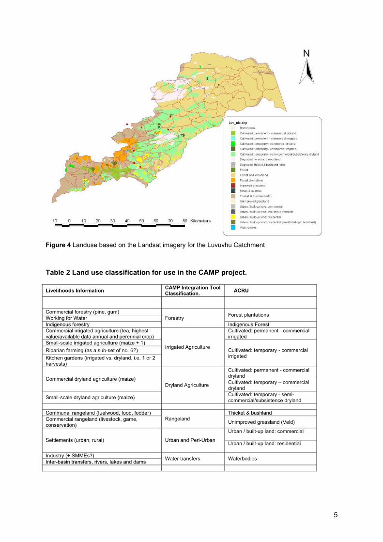
Land use The LANDSDAT TM 1996 coverage provided by the Council for Scientific and Industrial Research, CSIR was been used in a base input for the present land use (Figure 4). For the purposes of integrating this LANDSAT information with that collected in social surveys in the catchments, the land use classification shown in Table 1 and Table 2 has been utilised.

Table 1 Land Use in the Luvuvhu Catchment

Land Use Area commercial forestry estates 4%

subsistence agriculture and grazing 50%

cultivated lands - (including irrigated lands representing 3%) 13%

protected game reserve areas - 30%

urban areas 3%

5

Figure 4 Landuse based on the Landsat imagery for the Luvuvhu Catchment

Table 2 Land use classification for use in the CAMP project.

Livelihoods Information CAMP Integration Tool Classification. ACRU

Commercial forestry (pine, gum) Working for Water Forest plantations

Indigenous forestry Forestry

Indigenous Forest Commercial irrigated agriculture (tea, highest value/available data annual and perennial crop)

Cultivated: permanent - commercial irrigated

Small-scale irrigated agriculture (maize + 1) Riparian farming (as a sub-set of no. 6?) Kitchen gardens (irrigated vs. dryland, i.e. 1 or 2 harvests)

Irrigated Agriculture Cultivated: temporary - commercial irrigated

Cultivated: permanent - commercial dryland Commercial dryland agriculture (maize) Cultivated: temporary – commercial dryland

Small-scale dryland agriculture (maize)

Dryland Agriculture

Cultivated: temporary - semi-commercial/subsistence dryland

Communal rangeland (fuelwood, food, fodder) Thicket & bushland Commercial rangeland (livestock, game, conservation)

Rangeland Unimproved grassland (Veld)

Urban / built-up land: commercial Settlements (urban, rural) Urban and Peri-Urban Urban / built-up land: residential

Industry (+ SMMEs?) Inter-basin transfers, rivers, lakes and dams Water transfers Waterbodies

6

Based on soils surveys, it is estimated that 17% of the soils of the basins (960 280 ha) are potentially suitable for afforestation. However, only 14% of this area basin (14 750 ha) has been planted with commercial production. Rainfall constraints as well difficulties faced in obtaining a SFRA water use licence are the primary reasons for this. The bulk of irrigation water used in the catchment supplied either from the Albasini Government Water Scheme or from private dams. In contrast to many other areas of the country, significant areas of irrigation that rely on ground water do occur. DWAF (2002) reports that ground water is extensively over exploited, particularly in the vicinities of Albasini Dam and Thoyandou. Many small scale irrigation schemes are found. Most of these schemes utilize run-of-river flow and do not have any impounded water supply. It has been estimated that combined abstractions utilize all of the low flows in the river, particularly during the critically dry period of August to November. It has been suggested that there is good potential for further irrigation development in the catchment. However, DWAF (2002) suggest that future population growth in the WMA will be moderate and that the most likely increase in water demand is likely to come from the mining sector.

3.1 Dams

It has been estimated that dams regulate 55 million m3 of the 395 million m3 MAR in the catchment (DWAF, 2002). Four major dams, the Vondo Dam, the Tshakuma Dam, the Albasini Dam. and the recently completed Nandooni Dam, have a combined capacity of 40 million m3 (11% of the basin MAR).

3.2 Population and Water Demand

It is estimated that some 317 000 (1985) people depend on the basin for their water needs. Three major towns Thohoyandou (pop. 130 000), Louis Trichardt (pop.88 000) and Malamulele (2000) depend on the catchment for their water supply. It is estimated (1997) that urban and industrial use is 6% of the total water demand. However, it is predicted that this could reach 13% by 2010. Water use by commercial afforestation has been estimated at 10%. An amount of 2.4 x106 m3 per year is transferred to the town of Louis Trichardt in the Letaba catchment from the Albasini Dam. A low confidence estimate of ecological water requirements is 105 x 106 m3 per annum or 42% of MAR. Current estimates of water availability highlight that there is no surplus yield available in the water management area and that an over commitment of resources is shown to occur. This has been attributed to the provision made for the future implementation of ecological component of the Reserve.

4 INPUT DATA for HYDROLOGICAL MODELLING

Any land use sensitive rainfall-runoff model requires various input data. In addition to rainfall and estimates of PET, land use (including abstractions for domestic, agricultural and industrial use) and soils information are usually required, as is observed streamflow data to verify model output. In this phase, all necessary data required to run the model were sourced. Although adequate input data for an initial simulation were assimilated, this task is on going as further data are gathered and refined.

7

4.1 Streamflow Data

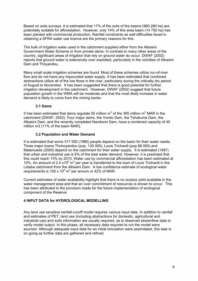
Daily streamflow data for the following weirs (A9H001, A9H002, A9H003, A9H004, A9H005, A9H006, A9H007, A9H012, A9H013 and A9H020), positions of which are illustrated in Figure 5, were obtained from Dept. Water Affairs and Forestry (DWAF) and the records were converted into a format suitable for use in models. The contributing areas for these weirs, as published by DWAF, are shown in Table 3 below together with the contributing area calculated from the CAMP GIS data

Figure 5 Streamflow gauges in the Luvuvhu Catchment.

Table 3 Luvuvhu Catchment streamflow gauging weirs and estimated upstream area.

Weir CAMP GIS Area DWAF Area % DiffA9H020 507.2 509.0 -0.36A9H005 609.3 611.0 -0.29A9H007 48.5 47.0 3.25A9H006 16.1 16.0 0.70A9H003 62.2 62.0 0.36A9H002 104.3 96.0 8.65A9H001 913.9 915.0 -0.12A9H012 1864.4 1758.0 6.05A9H004 328.9 320.0 2.78A9H013 1630.2 1429.0 14.08 .

The weirs that show discrepancies in contributing areas are those where some of the catchments could either flow into the Limpopo or into the Luvuvhu. However, due to the fairly arid nature of those areas the effect at the weirs is probably negligible.

4.2 Rainfall Data After a process of quality control and elimination, the best rainfall stations in the Luvuvhu area were chosen (Appendix I). These stations were used to provide rainfall data for all sub-

8

catchments using corrections for spatial and altitudinal differences. Rainfall data from the period 1957 to 1993 were extracted for use with hydrological models.

4.3 Potential Evaporation Routines for the estimation of daily maximum and minimum temperature values on a 1 x 1 grid of the country have been developed by Schulze (2003). These values have been obtained for the Luvuvhu Catchment and converted to daily Potential Evaporation values using the Linacre (1977) equation. See Appendix I for more details.

4.4 Land Use The aforementioned CSIR land use data (Figure 4, Table 2) was converted into values that could be used by the hydrological model. This is described in more detail in Appendix I (ACRU) and Appendix II (HYLUC). 5. Results As the hydrological modelling component of this study was intended to serve other study components, hydrological results are presented in those reports (Hope et al., 2003b; Fuller et al., 2003). However, some results are presented below for verification purposes, and to illustrate the hydrological response of current versus “natural” land use in the catchment.

5.1 Model Verification

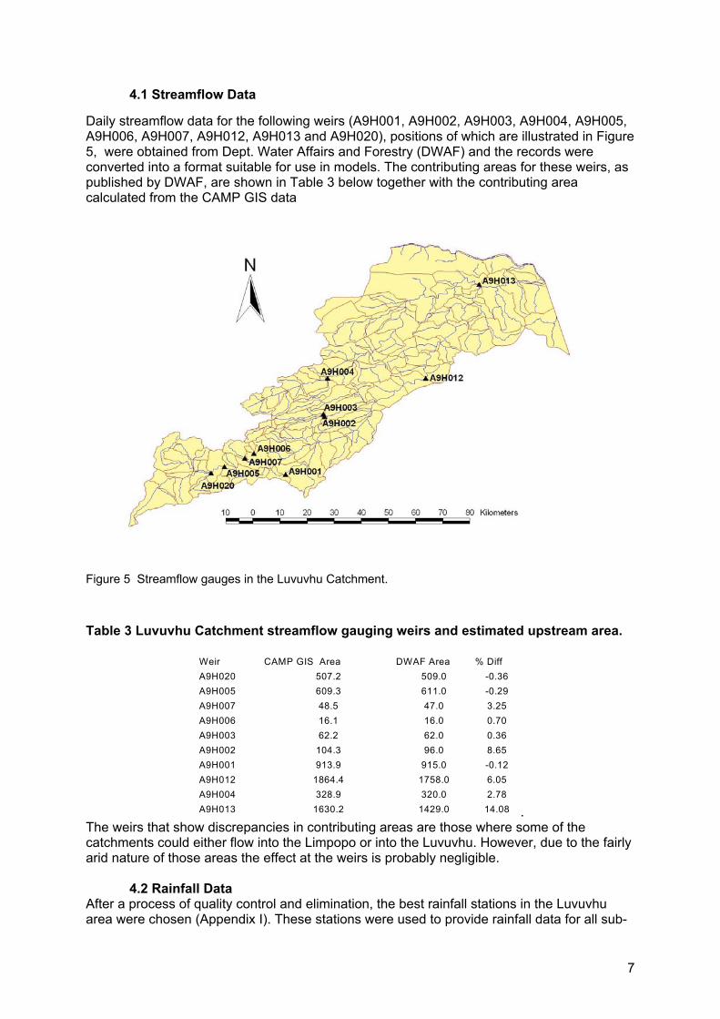
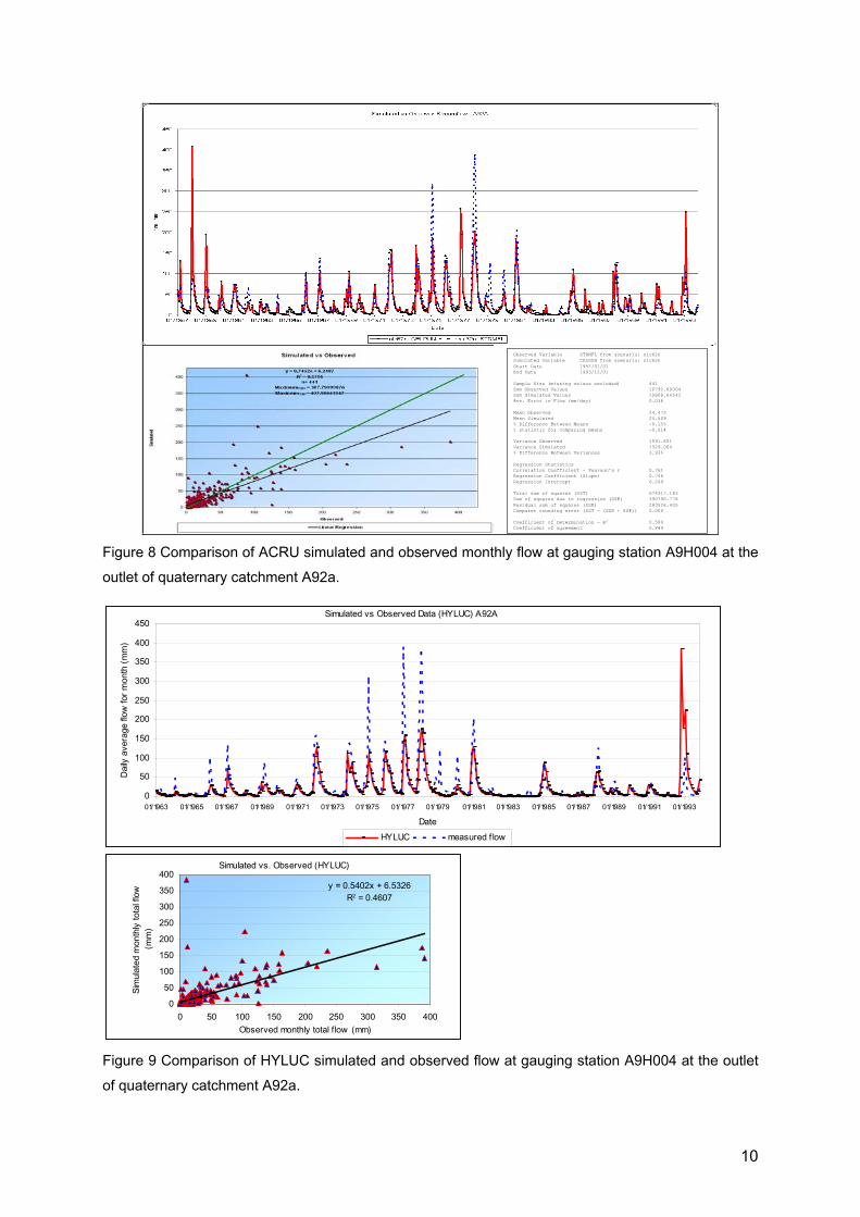
An important part of the hydrological modelling process is to establish that the streamflow simulated by the model is consistent with that of the physical system it represents. A model can only be applied with confidence once the model output has been tested for accuracy and correctness, i.e. verified, against observed data and where no observed data are available, to ensure that sensible values are generated. However, the poor quality of streamflow data in the Luvuvhu catchment and the lack of information regarding water abstractions has limited the effectiveness of such a verification exercise. Results from ACRU are presented for the weir A9H007. Figure 6 provides comparisons of daily simulated and observed flow values for A9H007 in the upper catchment of the Luvuvhu River from ACRU. Figure 7provides comparisons of daily simulated and observed flow values for A9H013 in the lower catchment of the Luvuvhu River from HYLUC. The quaternary catchment A92A on the Mutale river has been used as a focal study area in the CAMP project. In this case, comparisons of monthly flow are provided. Both the ACRU and HYLUC models simulate streamflow with a good correspondence to that observed, as illustrated by Figure 8 and Figure 9.

9

Observed Variable STRMFL from scenario: nlc33nSimulated Variable CELRUN from scenario: nlc33nStart Date 1957/01/01End Date 1993/12/31

Sample Size (missing values excluded) 13237Sum Observed Values 2593.200016Sum Simulated Values 5518.087633Ave. Error in Flow (mm/day) 0.221

Mean Observed 0.196Mean Simulated 0.417% Difference Between Means -112.79%t statistic for comparing means -18.670

Variance Observed 0.309Variance Simulated 1.545% Difference Between Variances -399.37%

Regression Statistics Correlation Coefficient - Pearson's r 0.479Regression Coefficient (Slope) 1.071Regression Intercept 0.207

Total sum of squares (SST) 20448.148Sum of squares due to regression (SSR) 4701.196Residual sum of squares (SSE) 15746.952Computer rounding error (SST - (SSR + SSE)) 0.000

Coefficient of Determination - R² 0.230 Coefficient of efficiency 0.197

Figure 6 Comparison of ACRU simulated and observed monthly flow at gauging station A9H007.

Simulated vs Observed Data (HYLUC) Whole Luvuvhu

0

5

10

15

20

25

30

35

40

45

50

11/1988 11/1990 11/1992

Date

Dai

ly a

vera

ge fl

ow fo

r mon

th (m

m)

HYLUC measured f low

Simulated vs. Observed (HYLUC)

y = 1.5387x + 1.0221R2 = 0.833

0

5

10

15

20

25

30

35

40

0 5 10 15 20 25 30 35 40Observed monthly total f low (mm)

Sim

ulat

ed m

onth

ly to

tal f

low

(m

m)

Figure 7 Comparison of HYLUC simulated and observed monthly flow at gauging station A9H013.

10

Observed Variable STRMFL from scenario: nlc62nSimulated Variable CELRUN from scenario: nlc62nStart Date 1957/01/01End Date 1993/12/01

Sample Size (missing values excluded) 441Sum Observed Values 10792.60004Sum Simulated Values 10808.64542Ave. Error in Flow (mm/day) 0.036

Mean Observed 24.473Mean Simulated 24.509% Difference Between Means -0.15%t statistic for comparing means -0.014

Variance Observed 1591.651Variance Simulated 1529.064% Difference Between Variances 3.93%

Regression Statistics Correlation Coefficient - Pearson's r 0.761Regression Coefficient (Slope) 0.746Regression Intercept 6.249

Total sum of squares (SST) 674317.183Sum of squares due to regression (SSR) 390790.778Residual sum of squares (SSE) 283526.405Computer rounding error (SST - (SSR + SSE)) 0.000

Coefficient of Determination - R² 0.580 Coefficient of agreement 0.849

Figure 8 Comparison of ACRU simulated and observed monthly flow at gauging station A9H004 at the

outlet of quaternary catchment A92a.

Simulated vs Observed Data (HYLUC) A92A

0

50

100

150

200

250

300

350

400

450

01/1963 01/1965 01/1967 01/1969 01/1971 01/1973 01/1975 01/1977 01/1979 01/1981 01/1983 01/1985 01/1987 01/1989 01/1991 01/1993

Date

Dai

ly a

vera

ge fl

ow fo

r mon

th (m

m)

HYLUC measured f low

Simulated vs. Observed (HYLUC)

y = 0.5402x + 6.5326R2 = 0.4607

0

50

100

150

200

250

300

350

400

0 50 100 150 200 250 300 350 400Observed monthly total f low (mm)

Sim

ulat

ed m

onth

ly to

tal f

low

(m

m)

Figure 9 Comparison of HYLUC simulated and observed flow at gauging station A9H004 at the outlet

of quaternary catchment A92a.

11

5.2 Current versus “Natural” Land use

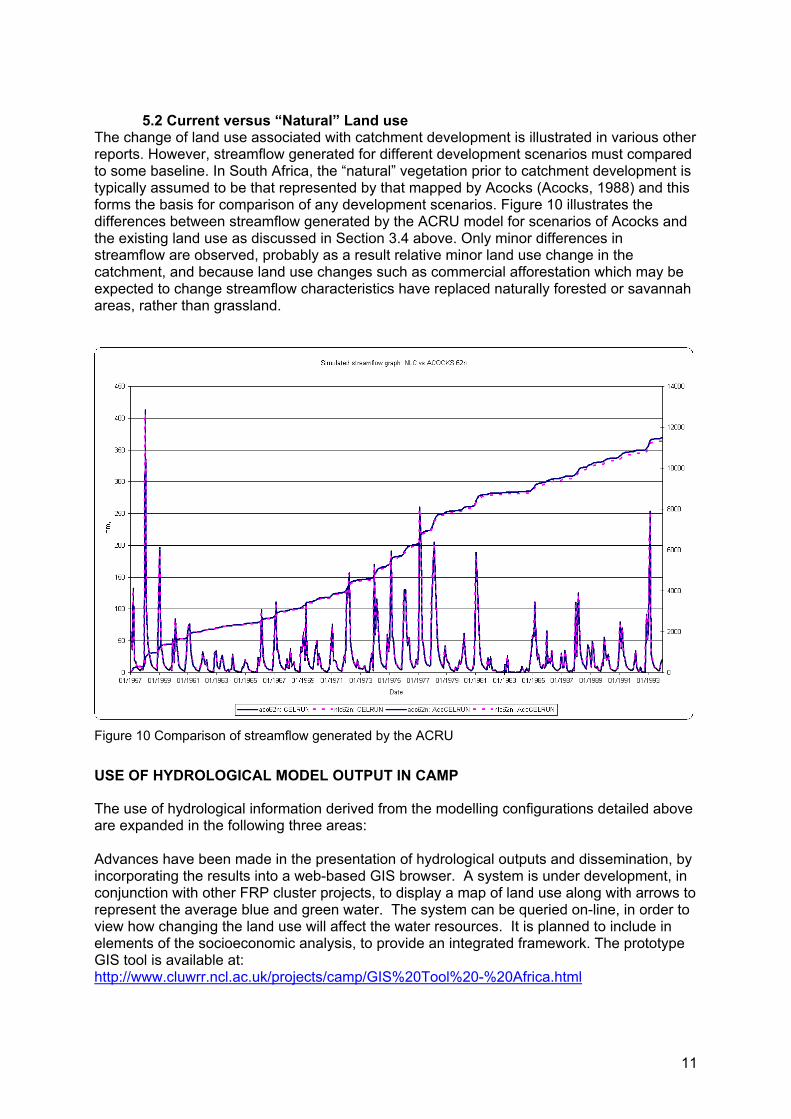
The change of land use associated with catchment development is illustrated in various other reports. However, streamflow generated for different development scenarios must compared to some baseline. In South Africa, the “natural” vegetation prior to catchment development is typically assumed to be that represented by that mapped by Acocks (Acocks, 1988) and this forms the basis for comparison of any development scenarios. Figure 10 illustrates the differences between streamflow generated by the ACRU model for scenarios of Acocks and the existing land use as discussed in Section 3.4 above. Only minor differences in streamflow are observed, probably as a result relative minor land use change in the catchment, and because land use changes such as commercial afforestation which may be expected to change streamflow characteristics have replaced naturally forested or savannah areas, rather than grassland.

Figure 10 Comparison of streamflow generated by the ACRU

USE OF HYDROLOGICAL MODEL OUTPUT IN CAMP

The use of hydrological information derived from the modelling configurations detailed above are expanded in the following three areas: Advances have been made in the presentation of hydrological outputs and dissemination, by incorporating the results into a web-based GIS browser. A system is under development, in conjunction with other FRP cluster projects, to display a map of land use along with arrows to represent the average blue and green water. The system can be queried on-line, in order to view how changing the land use will affect the water resources. It is planned to include in elements of the socioeconomic analysis, to provide an integrated framework. The prototype GIS tool is available at: http://www.cluwrr.ncl.ac.uk/projects/camp/GIS%20Tool%20-%20Africa.html

12

APPENDIX I

CONFIGURATION OF THE ACRU AGROHYDROLOGICAL MODELLING SYSTEM FOR THE LUVUVHU CATCHMENT

1. The ACRU Agrohydrological Modelling System (http://www.beeh.unp.ac.za/acru)

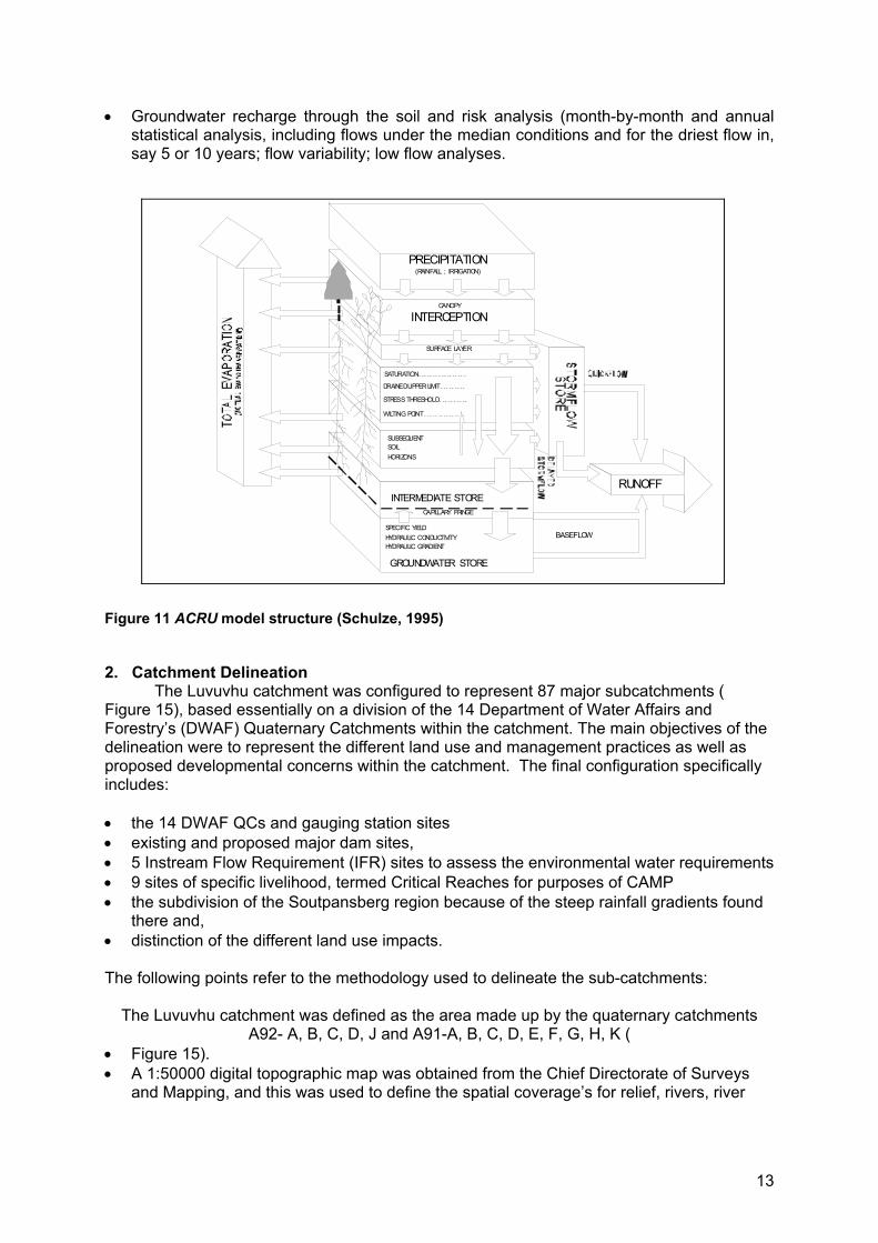
ACRU is a daily time step, physical-conceptual model revolving around multi-layer soil water budgeting. It is a multi-purpose model with options to output, inter alia, daily values of streamflow, peak discharges, recharge to ground water, reservoir status, irrigation water supply and demand as well as seasonal crop yields. The model is structured (Figure 11) to be hydrologically sensitive to catchment land uses and changes thereof, including the impacts of proposed developments, such as large dams, on catchment streamflow and sediment generation, as well as the streamflow regime. The model requires input of known, measurable, factors including information on: • climate (daily rainfall; temperature; potential evaporation) • soils (horizon depths; soil water retention; drainage characteristics) • commercially planted tree species (species distributions; levels of site preparation) • other dryland land uses (crops; management level; areas; above- and below-ground

vegetation characteristics) • dams (capacities; surface areas; releases; abstractions) • irrigation practices (crop type/seasonality; mode of scheduling; areas; sources of water;

application efficiencies) and • other abstractions (e.g. domestic or livestock; amounts; sources of water; seasonality) This information is transformed in the model by considering: • the climate, soil, vegetative, hydrological and human subsystems • how they interact with on another • what thresholds are required for responses to take place • how the various responses lag at different rates and • whether there are feed-forwards and feedbacks which allow the system to respond in a

positive or reverse direction The model then produces output of the unmeasured variables to be assessed, e.g. • Streamflows (from different parts of the catchment; including stormflow and baseflow on

a daily basis) and low flows

13

• Groundwater recharge through the soil and risk analysis (month-by-month and annual statistical analysis, including flows under the median conditions and for the driest flow in, say 5 or 10 years; flow variability; low flow analyses.

Figure 11 ACRU model structure (Schulze, 1995)

2. Catchment Delineation

The Luvuvhu catchment was configured to represent 87 major subcatchments ( Figure 15), based essentially on a division of the 14 Department of Water Affairs and Forestry’s (DWAF) Quaternary Catchments within the catchment. The main objectives of the delineation were to represent the different land use and management practices as well as proposed developmental concerns within the catchment. The final configuration specifically includes: • the 14 DWAF QCs and gauging station sites • existing and proposed major dam sites, • 5 Instream Flow Requirement (IFR) sites to assess the environmental water requirements • 9 sites of specific livelihood, termed Critical Reaches for purposes of CAMP • the subdivision of the Soutpansberg region because of the steep rainfall gradients found

there and, • distinction of the different land use impacts. The following points refer to the methodology used to delineate the sub-catchments:

The Luvuvhu catchment was defined as the area made up by the quaternary catchments A92- A, B, C, D, J and A91-A, B, C, D, E, F, G, H, K (

• Figure 15). • A 1:50000 digital topographic map was obtained from the Chief Directorate of Surveys

and Mapping, and this was used to define the spatial coverage’s for relief, rivers, river

RUNOFF

PRECIPITATION(RAINFALL ; IRRIGATION)

BASEFLOW

INTERMEDIATE STORE

SURFACE LAYER

SUBSEQUENTSOILHORIZONS

DRAINED UPPER LIMIT . . . . . . . . .

SATURATION . . . . . . . . . . . . . . . . .

WILTING POINT . . . . . . . . . . . . . . .

STRESS THRESHOLD . . . . . . . . . .

GROUNDWATER STORE

SPECIFIC YIELD

HYDRAULIC GRADIENT

CAPILLARY FRINGE

HYDRAULIC CONDUCTIVITY

INTERCEPTIONCANOPY

14

areas, water bodies, roads, dam walls and schools within the Luvuvhu catchment boundary.

• Some problems were experienced with the water bodies’ coverage. Lake Funduduzi (a well-known sacred site in the area) was not included, and some of the other dams in the catchment (including the Vondo Dam) did not seem to be included. A polygon representing the area of Lake Funduduzi was subsequently added to the coverage using the well-defined contours of the relief coverage as a guide.

• The quaternary catchments were then further divided into 86 sub-catchments, which facilitated ACRU model set-up. These were hydrological delineations (i.e. the outlets of the subcatchments were at hydrologically significant locations within the catchment, such as weirs). Sub-catchments were also kept to a size optimal to model performance (5-350km²).

• The following indicators were used to define subcatchments outlets: - Dams from the water bodies’ coverage together with a list of 6 dams that were

highlighted as being the important dams within the catchment, - All the measuring weirs that are within the List of Hydrological Gauging Stations July

1990 Volume 1 (DWAF, 1990), - The sites where water quality is measured by the CSIR, and - All the tributaries that are included in the State of the Rivers Report 2001 (some of

the sites that were used to determine ‘river health’ were also used to delineate the subcatchments).

An approximate location of the Xikundu weir was only received after the catchment delineation had been completed, however the outlet point of the relevant catchment (41) was deemed to be acceptably close to the actual position of the weir so the delineation was kept unchanged.

• Some areas of the catchment don’t flow into the Luvuvhu but flow directly into the Limpopo River instead. These areas were all divided into their own subcatchments. A theoretical sub-catchment 87 was created to represent the Limpopo River.

• In the Northern parts of the catchment it proved very difficult to delineate the catchment, as there were large flat areas where it was very difficult to determine whether the basin contributed to the Limpopo River or the Luvuvhu River. The possibility exists to re-route flow from these catchments should this be deemed necessary.

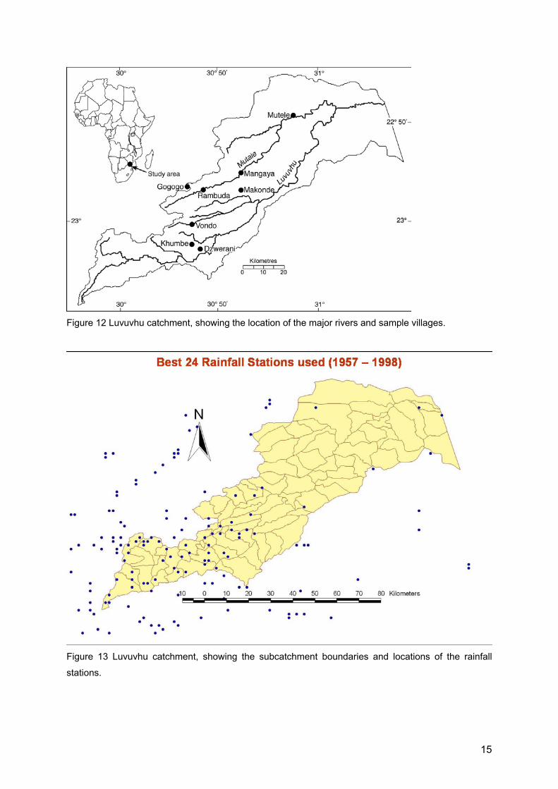
• A map of the Luvuvhu catchment, showing major rivers and the locations of the sample villages is shown in Figure 12.

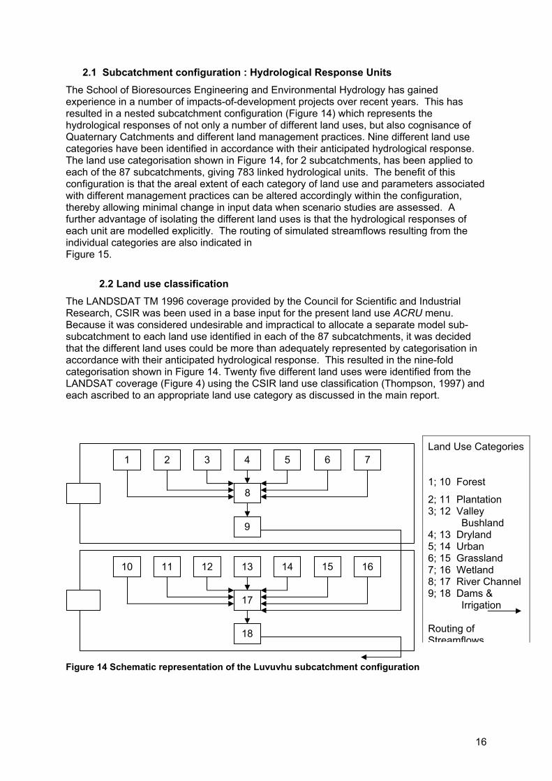
• A map showing the sub-catchments and locations of the rainfall stations is shown in Figure 13.

• Schematics representing the routing of all the subcatchments are illustrated in • Figure 15.

15

Figure 12 Luvuvhu catchment, showing the location of the major rivers and sample villages.

Figure 13 Luvuvhu catchment, showing the subcatchment boundaries and locations of the rainfall

stations.

16

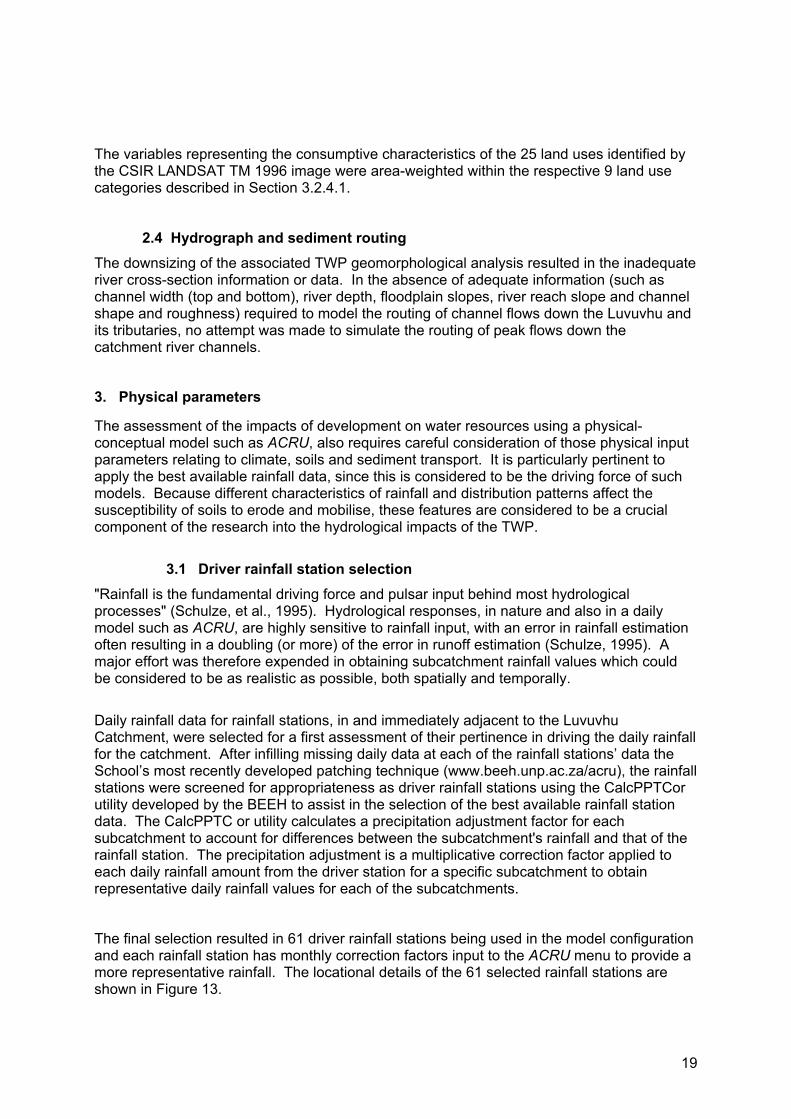
2.1 Subcatchment configuration : Hydrological Response Units The School of Bioresources Engineering and Environmental Hydrology has gained experience in a number of impacts-of-development projects over recent years. This has resulted in a nested subcatchment configuration (Figure 14) which represents the hydrological responses of not only a number of different land uses, but also cognisance of Quaternary Catchments and different land management practices. Nine different land use categories have been identified in accordance with their anticipated hydrological response. The land use categorisation shown in Figure 14, for 2 subcatchments, has been applied to each of the 87 subcatchments, giving 783 linked hydrological units. The benefit of this configuration is that the areal extent of each category of land use and parameters associated with different management practices can be altered accordingly within the configuration, thereby allowing minimal change in input data when scenario studies are assessed. A further advantage of isolating the different land uses is that the hydrological responses of each unit are modelled explicitly. The routing of simulated streamflows resulting from the individual categories are also indicated in Figure 15.

2.2 Land use classification The LANDSDAT TM 1996 coverage provided by the Council for Scientific and Industrial Research, CSIR was been used in a base input for the present land use ACRU menu. Because it was considered undesirable and impractical to allocate a separate model sub-subcatchment to each land use identified in each of the 87 subcatchments, it was decided that the different land uses could be more than adequately represented by categorisation in accordance with their anticipated hydrological response. This resulted in the nine-fold categorisation shown in Figure 14. Twenty five different land uses were identified from the LANDSAT coverage (Figure 4) using the CSIR land use classification (Thompson, 1997) and each ascribed to an appropriate land use category as discussed in the main report.

Figure 14 Schematic representation of the Luvuvhu subcatchment configuration

Land Use Categories

1; 10 Forest

2; 11 Plantation 3; 12 Valley Bushland 4; 13 Dryland 5; 14 Urban 6; 15 Grassland 7; 16 Wetland 8; 17 River Channel 9; 18 Dams & Irrigation Routing of Streamflows

9

8

1 2 3 4 5 7 6

10 11 12 13 14 16

17

18

15

17

2.3 Vegetative water use The vegetative water use by each land use within the 9 land categories is assessed using the values described by Smithers and Schulze (1995). The water use by each land use includes: • an interception loss value, which can change from month to month during a plant's

annual growth cycle, to account for the estimated interception of rainfall by the plant's canopy on a rainday,

• a monthly consumptive water use (or "crop") coefficient (converted internally in the model to daily values by Fourier Analysis), which reflects the ratio of water use by vegetation under conditions of freely available soil water to the evaporation from a reference potential evaporation (e.g. A-pan or equivalent), and

• the fraction of plant roots that are active in extracting soil moisture from the topsoil horizon in a given month, this fraction being linked to root growth patterns during a year and periods of senescence brought on, for example, by a lack of soil moisture or by frost.

A further variable which can change seasonally is the coefficient of the initial abstraction (cIa), where, in stormflow generation, the cIa accounts for depression storage and initial infiltration before stormflow commences. In the ACRU model this coefficient takes cognisance of surface roughness (e.g. after ploughing) and initial infiltration before stormflow commences. Higher values of cIa under forests, for example, reflect enhanced infiltration while lower values on veld in summer months are the result of higher rainfall intensities (and consequent lower initial infiltrations) experienced during the thunderstorm season.

18

Figure 15 – ACRU catchment configuration for the Luvuvhu

2120

12

8765

14

17

16

15

1310

11

3

9

421

19

18

A9H007 A9H006

A9H

020

A91A & A91B

A91C

A91E

A91D

Albasini Dam

Tshukoma Dam

Gauging Stations

Dams

33

46

26

22 302725 322423

45

41 47

3129

28

444342

40

32

37

393835 3617

13

40

21

34

A9H001

A9H003A9H

002

A91F

A91G

A91H

A9H

012Vondo Dam

Phipidi Dam

Damini Dam

Nandoni Dam

53

55

61

58

59 62

5452

51

60

5756

50494847

65

696867666463

A92J

A92A A92B

A9H

004

69

55

79

87

83

79787776

7572

74737170

80 81

86

84

82

85

87

A9H

013

19

The variables representing the consumptive characteristics of the 25 land uses identified by the CSIR LANDSAT TM 1996 image were area-weighted within the respective 9 land use categories described in Section 3.2.4.1.

2.4 Hydrograph and sediment routing The downsizing of the associated TWP geomorphological analysis resulted in the inadequate river cross-section information or data. In the absence of adequate information (such as channel width (top and bottom), river depth, floodplain slopes, river reach slope and channel shape and roughness) required to model the routing of channel flows down the Luvuvhu and its tributaries, no attempt was made to simulate the routing of peak flows down the catchment river channels.

3. Physical parameters

The assessment of the impacts of development on water resources using a physical-conceptual model such as ACRU, also requires careful consideration of those physical input parameters relating to climate, soils and sediment transport. It is particularly pertinent to apply the best available rainfall data, since this is considered to be the driving force of such models. Because different characteristics of rainfall and distribution patterns affect the susceptibility of soils to erode and mobilise, these features are considered to be a crucial component of the research into the hydrological impacts of the TWP.

3.1 Driver rainfall station selection "Rainfall is the fundamental driving force and pulsar input behind most hydrological processes" (Schulze, et al., 1995). Hydrological responses, in nature and also in a daily model such as ACRU, are highly sensitive to rainfall input, with an error in rainfall estimation often resulting in a doubling (or more) of the error in runoff estimation (Schulze, 1995). A major effort was therefore expended in obtaining subcatchment rainfall values which could be considered to be as realistic as possible, both spatially and temporally.

Daily rainfall data for rainfall stations, in and immediately adjacent to the Luvuvhu Catchment, were selected for a first assessment of their pertinence in driving the daily rainfall for the catchment. After infilling missing daily data at each of the rainfall stations’ data the School’s most recently developed patching technique (www.beeh.unp.ac.za/acru), the rainfall stations were screened for appropriateness as driver rainfall stations using the CalcPPTCor utility developed by the BEEH to assist in the selection of the best available rainfall station data. The CalcPPTC or utility calculates a precipitation adjustment factor for each subcatchment to account for differences between the subcatchment's rainfall and that of the rainfall station. The precipitation adjustment is a multiplicative correction factor applied to each daily rainfall amount from the driver station for a specific subcatchment to obtain representative daily rainfall values for each of the subcatchments.

The final selection resulted in 61 driver rainfall stations being used in the model configuration and each rainfall station has monthly correction factors input to the ACRU menu to provide a more representative rainfall. The locational details of the 61 selected rainfall stations are shown in Figure 13.

20

3.2 Soils Soils play a crucial role in catchments' hydrological responses by: • facilitating the infiltration of precipitation, and thereby largely controlling stormflow

generation, • acting as a store of water which makes soil water available to plants • redistributing water, both within the soil profile and out of it, • evaporation and transpiration processes and • drainage below the root zone and eventually into the groundwater zone which feeds

baseflow.

The GIS coverage of soil Land Types for the Luvuvhu Catchment was obtained from the Institute for Soil, Climate and Water (ISCW). For each Land Type a vast amount of information on percentages of soil series per terrain unit, soils depths, texture properties and drainage limiting properties was provided by the ISCW. This Land Type information had to be "translated" into the hydrological soils input properties for a two-horizon soil profile, as required by ACRU. This translation takes place via a Soils Decisions Support System computer program called AUTOSOILS, developed from information contained in Schulze (1995). See www.beeh.unp.ac.za/acru/utilities for more details.

AUTOSOILS output includes the thickness of the topsoil and subsoil horizons, values of the soil water content at permanent wilting point, drained upper limit and saturation (porosity) for both soil layers, as well as saturated drainage redistribution rates. Values of the above variables were determined for each soil series making up a Land Type and then area-weighted according to the proportions of each soil series in a Land Type and then the proportions of each Land Type found in a subcatchment. An average dominant texture class of sandy clay loam was assumed for all subcatchments. Output from AUTOSOILS also contains runoff related values, derived from Land Type information, of two further variables, viz. fractions of adjunct impervious areas within a subcatchment, constituting the areas around channel zones assumed to be permanently wet and from which direct overland flow is hypothesised to occur after a rainfall event, and disjunct impervious areas such as rock outcrops, from which rainfall running off infiltrates into surrounding areas and influences their water budgets. The final subcatchment values of soil textures, top- and subsoil horizon thickness, retention constants at critical soil water contents, drainage rates and percentages of impervious areas for each of the subcatchments was included in the ACRU input "menu" file. 3 Water allocations and abstractions To effectively assess the impacts of any water resource development on the generation of streamflows and sediment yields, it is necessary to simulate the conditions which satisfy the Reserve (RSA, 1998) as well as any direct anthropogenic streamflow abstractions performed within the Catchment. For the purpose of this study these were viewed as comprising two basic water allocations, viz: • environmental requirements and

• irrigation and domestic abstractions

4.1 Environmental requirements : instream flow requirements

The determination, and fulfilment, of the ecological reserve for the Luvuvhu Catchment is a major issue of concern. Much preparatory work has already been conducted to determine

21

the Instream Flow Requirements (IFRs) for the Luvuvhu Rivers and its tributaries. However, to date, no comprehensive IFR estimation has been performed.

4.2 Irrigation and domestic abstractions There is a paucity of information available to perform the necessary ACRU irrigation modules for the Luvuvhu catchment. For this reason, assumptions were made to simulate effective irrigation abstraction. A similar situation prevails for the simulation of domestic abstractions. Consequently this factor was omitted from the base menu simulations

4.3 Systems Operation : dam operating rules The level of dam operating rules required for the operation of the ACRU model were not available. 5. Uncertainties and refinements • There have been problems obtaining information on the dams within each sub-

catchment. More time needs to be spent on obtaining additional information on dams. • Lake Fundudzi has no overflow and all the water that leaves the lake flows into the

ground water. There are apparently 2 natural springs a few hundred meters downstream of the lake. It is not clear what proportion of the flow out of the lake is represented by these springs.

• Daily flows for 4 canals (A9H015, A9H016, A9H017, A9H018, A9H023 [17 and 18 are at the same site]) were received, which represent river abstractions. These daily flows were converted to monthly flows in these canals. These values were then assumed to be domestic abstractions as no further explanatory data was available. These represent the only abstraction data obtained so far.

• Only very course data on irrigation within the catchment was available (obtained from the WR90 report). More specific information needs be sourced regarding irrigation.

• The next phase is to perhaps create a current land use menu for the next model run. Once all the irrigation, reservoir and abstraction information has been found the final menu can be set up and fine tuned to get it as close as is needed for the final set of runs.

22

APPENDIX II

CONFIGURATION OF THE HYLUCAGROHYDROLOGICAL MODELLING SYSTEM FOR THE LUVUVHU CATCHMENT

1. The HYLUC Agrohydrological Modelling System

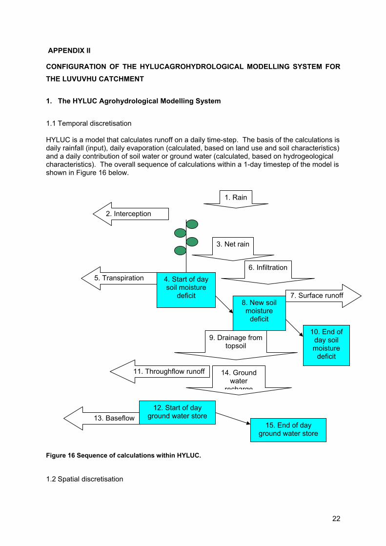
1.1 Temporal discretisation HYLUC is a model that calculates runoff on a daily time-step. The basis of the calculations is daily rainfall (input), daily evaporation (calculated, based on land use and soil characteristics) and a daily contribution of soil water or ground water (calculated, based on hydrogeological characteristics). The overall sequence of calculations within a 1-day timestep of the model is shown in Figure 16 below.

Figure 16 Sequence of calculations within HYLUC.

1.2 Spatial discretisation

1. Rain

4. Start of day soil moisture

deficit

2. Interception

3. Net rain

5. Transpiration

7. Surface runoff

6. Infiltration

8. New soil moisture

deficit

9. Drainage from topsoil

10. End of day soil moisture

deficit

11. Throughflow runoff 14. Ground water

recharge

15. End of day ground water store

13. Baseflow 12. Start of day

ground water store

23

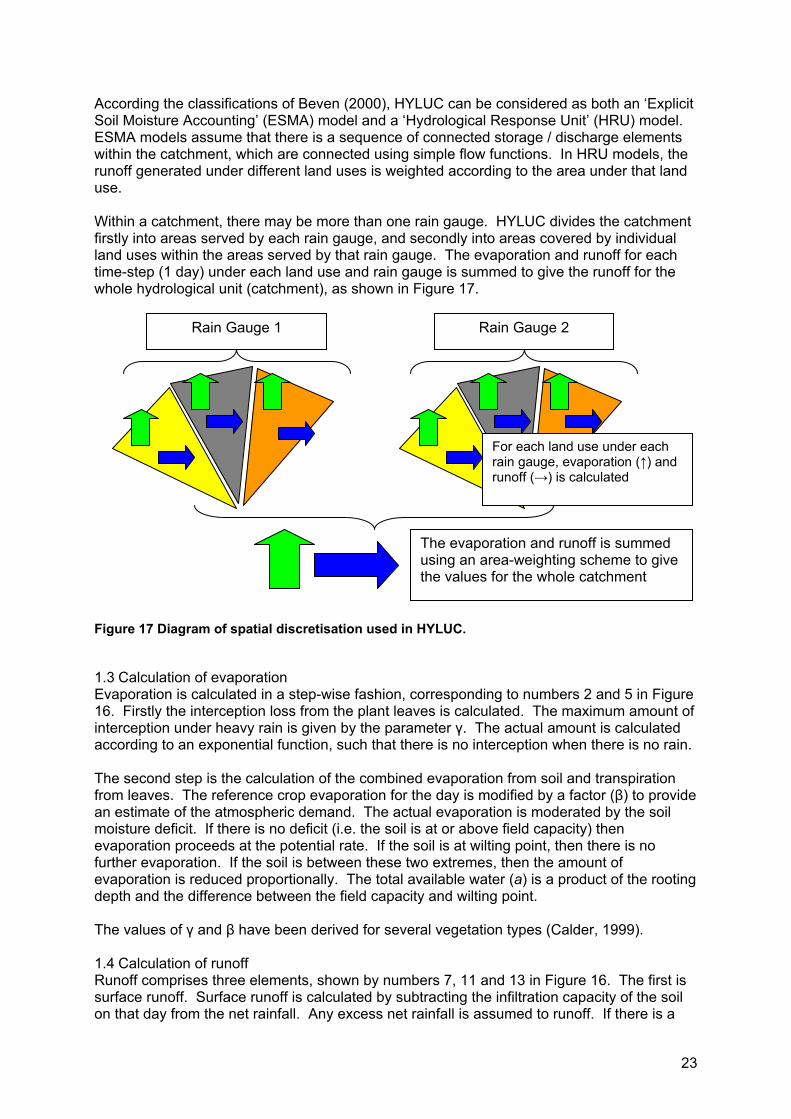
According the classifications of Beven (2000), HYLUC can be considered as both an ‘Explicit Soil Moisture Accounting’ (ESMA) model and a ‘Hydrological Response Unit’ (HRU) model. ESMA models assume that there is a sequence of connected storage / discharge elements within the catchment, which are connected using simple flow functions. In HRU models, the runoff generated under different land uses is weighted according to the area under that land use. Within a catchment, there may be more than one rain gauge. HYLUC divides the catchment firstly into areas served by each rain gauge, and secondly into areas covered by individual land uses within the areas served by that rain gauge. The evaporation and runoff for each time-step (1 day) under each land use and rain gauge is summed to give the runoff for the whole hydrological unit (catchment), as shown in Figure 17.

Figure 17 Diagram of spatial discretisation used in HYLUC.

1.3 Calculation of evaporation Evaporation is calculated in a step-wise fashion, corresponding to numbers 2 and 5 in Figure 16. Firstly the interception loss from the plant leaves is calculated. The maximum amount of interception under heavy rain is given by the parameter γ. The actual amount is calculated according to an exponential function, such that there is no interception when there is no rain. The second step is the calculation of the combined evaporation from soil and transpiration from leaves. The reference crop evaporation for the day is modified by a factor (β) to provide an estimate of the atmospheric demand. The actual evaporation is moderated by the soil moisture deficit. If there is no deficit (i.e. the soil is at or above field capacity) then evaporation proceeds at the potential rate. If the soil is at wilting point, then there is no further evaporation. If the soil is between these two extremes, then the amount of evaporation is reduced proportionally. The total available water (a) is a product of the rooting depth and the difference between the field capacity and wilting point. The values of γ and β have been derived for several vegetation types (Calder, 1999). 1.4 Calculation of runoff Runoff comprises three elements, shown by numbers 7, 11 and 13 in Figure 16. The first is surface runoff. Surface runoff is calculated by subtracting the infiltration capacity of the soil on that day from the net rainfall. Any excess net rainfall is assumed to runoff. If there is a

Rain Gauge 1 Rain Gauge 2

For each land use under each rain gauge, evaporation (↑) and runoff (→) is calculated

The evaporation and runoff is summed using an area-weighting scheme to give the values for the whole catchment

24

soil moisture deficit, then infiltration is assumed to proceed at the maximum rate. If the soil moisture content is above field capacity, then the infiltration rate is reduced. The second stage of calculation of runoff is throughflow runoff. Water in the soil that is held above field capacity will drain out of the soil over time (following a first-order kinetic). This water is partitioned between water that reaches surface water and water that contributes to ground water recharge. The ground water recharge is restricted to a maximum value by an exponential function. Throughflow runoff is the difference between the water draining from the soil and the ground water recharge. The third stage of calculation of runoff is baseflow. Baseflow consists of ground water that seeps from the phreatic zone into rivers according to the amount of water in the ground water and a first-order recharge rate. The input parameters are generally related to physically measurable characteristics, but they cannot be viewed in purely empirical terms. Catchments are spatially variable, so a characteristic in one area of the catchment may not represent the whole catchment. Given a large-enough data set, it would be theoretically possible to derive an integrated value for each of the parameters. However, the weightings that are attached to spatial data are not obvious. For example, soils near the top of the catchment may require a different weighting from soils near the outflow of the catchment. Furthermore, appropriate weightings may depend on the season. Therefore, the descriptions below can be used as guides, but should not be used too rigidly. The ultimate definition of the catchment response to rainfall is what can be measured in the rivers at the base of the catchment. Therefore, it is acceptable to calibrate the parameters if appropriate data are available from the catchment. In this project, the values used were obtained from a simple calibration according to the outflow data from the Tengwe (A92A) subcatchment. 2. Catchment Delineation The catchment was configured more simply than for the ACRU model (Appendix 1), but based on the same underlying data. The 14 quaternary catchments (QC) from DWAF were used as the main division of the Luvuvhu secondary catchment. Each QC was treated as a hydrological response unit. The Luvuvhu catchment was defined as the area made up by the QCs A92- A, B, C, D, J and A91-A, B, C, D, E, F, G, H, K. In particular, the quaternary catchment A92A (Tengwe) was used as a special study area because a good flow data set was available for this QC, and this QC is at the top of the whole Luvuvhu catchment so there is no in-flow from upstream QCs.

2.1 Land use classification The LANDSDAT TM 1996 coverage provided by the Council for Scientific and Industrial Research, CSIR was been used in a base input for the HYLUC land use information. The 25 different land uses were lumped into 6 ‘summary’ land uses as described in the main report. The summary land uses were:

• dryland agriculture

• irrigated agriculture

• forestry

• bushland / rangeland

• urban and periurban

• water bodies

25

Analysis of scenarios was performed by changing the proportions of the above land uses to account for changing land use.

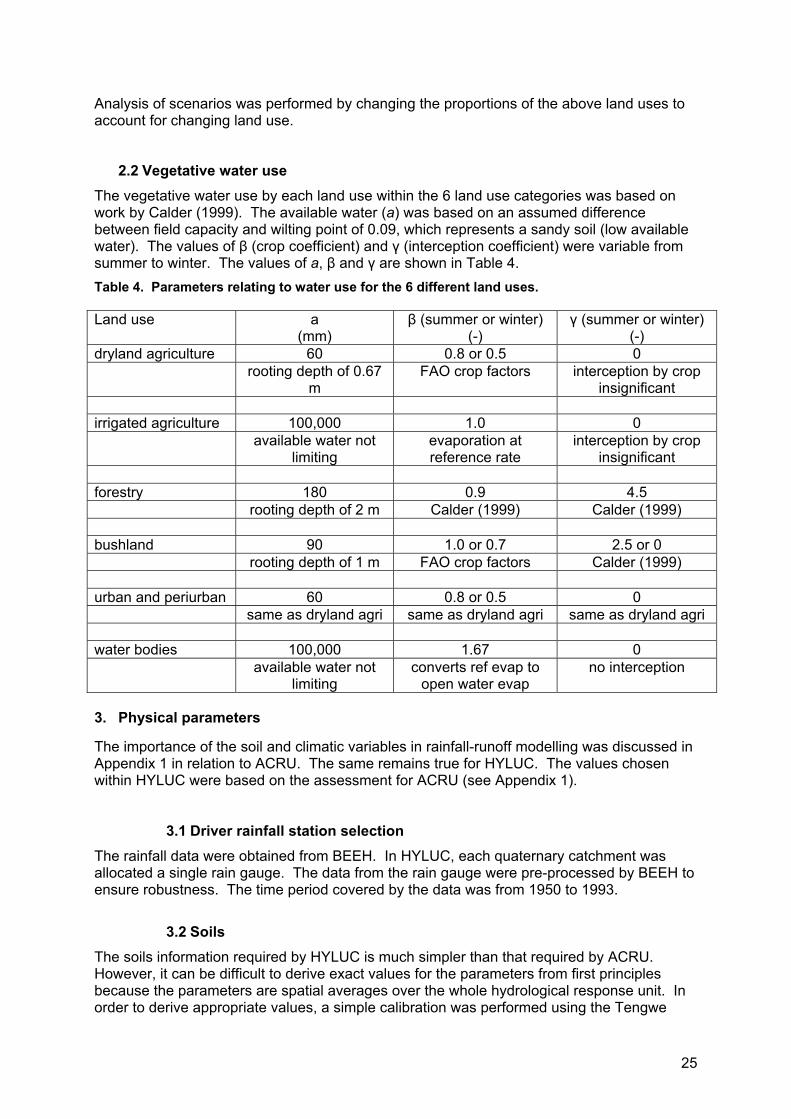
2.2 Vegetative water use The vegetative water use by each land use within the 6 land use categories was based on work by Calder (1999). The available water (a) was based on an assumed difference between field capacity and wilting point of 0.09, which represents a sandy soil (low available water). The values of β (crop coefficient) and γ (interception coefficient) were variable from summer to winter. The values of a, β and γ are shown in Table 4. Table 4. Parameters relating to water use for the 6 different land uses.

Land use a (mm)

β (summer or winter) (-)

γ (summer or winter) (-)

dryland agriculture 60 0.8 or 0.5 0 rooting depth of 0.67

m FAO crop factors interception by crop

insignificant irrigated agriculture 100,000 1.0 0 available water not

limiting evaporation at reference rate

interception by crop insignificant

forestry 180 0.9 4.5 rooting depth of 2 m Calder (1999) Calder (1999) bushland 90 1.0 or 0.7 2.5 or 0 rooting depth of 1 m FAO crop factors Calder (1999) urban and periurban 60 0.8 or 0.5 0 same as dryland agri same as dryland agri same as dryland agri water bodies 100,000 1.67 0 available water not

limiting converts ref evap to

open water evap no interception

3. Physical parameters

The importance of the soil and climatic variables in rainfall-runoff modelling was discussed in Appendix 1 in relation to ACRU. The same remains true for HYLUC. The values chosen within HYLUC were based on the assessment for ACRU (see Appendix 1).

3.1 Driver rainfall station selection The rainfall data were obtained from BEEH. In HYLUC, each quaternary catchment was allocated a single rain gauge. The data from the rain gauge were pre-processed by BEEH to ensure robustness. The time period covered by the data was from 1950 to 1993.

3.2 Soils The soils information required by HYLUC is much simpler than that required by ACRU. However, it can be difficult to derive exact values for the parameters from first principles because the parameters are spatial averages over the whole hydrological response unit. In order to derive appropriate values, a simple calibration was performed using the Tengwe

26

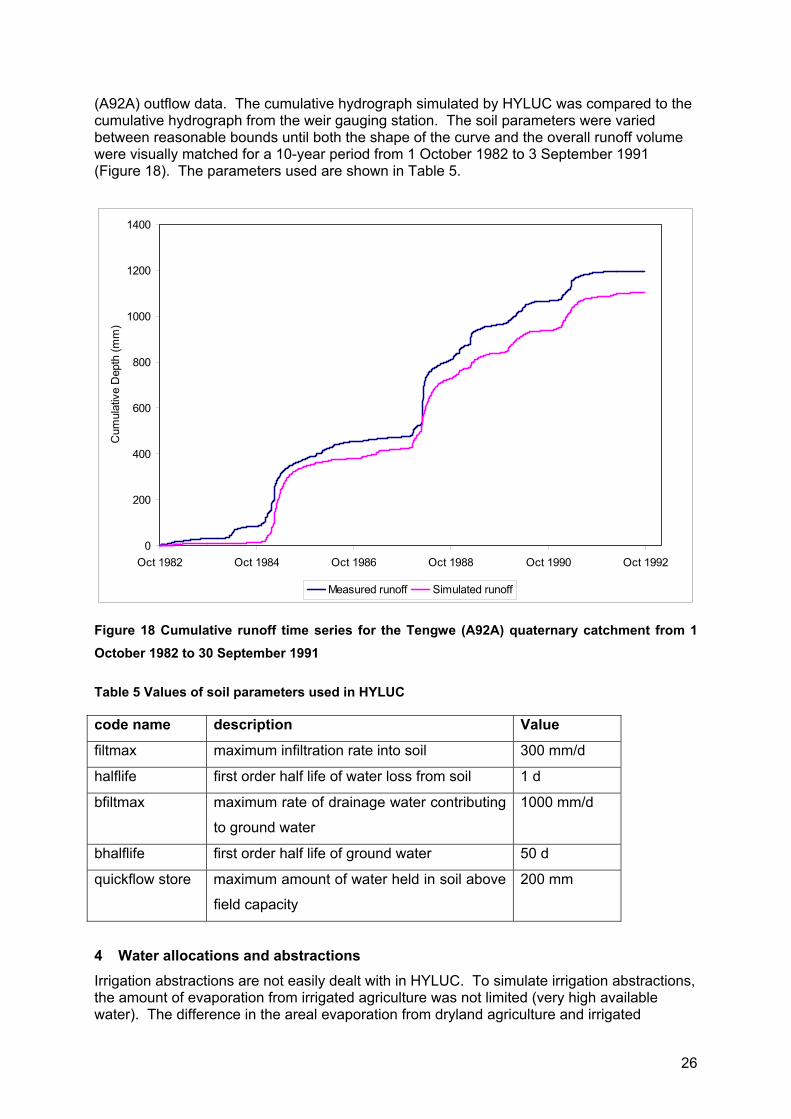
(A92A) outflow data. The cumulative hydrograph simulated by HYLUC was compared to the cumulative hydrograph from the weir gauging station. The soil parameters were varied between reasonable bounds until both the shape of the curve and the overall runoff volume were visually matched for a 10-year period from 1 October 1982 to 3 September 1991 (Figure 18). The parameters used are shown in Table 5.

0

200

400

600

800

1000

1200

1400

Oct 1982 Oct 1984 Oct 1986 Oct 1988 Oct 1990 Oct 1992

Cum

ulat

ive

Dep

th (m

m)

Measured runoff Simulated runoff

Figure 18 Cumulative runoff time series for the Tengwe (A92A) quaternary catchment from 1 October 1982 to 30 September 1991

Table 5 Values of soil parameters used in HYLUC

code name description Value

filtmax maximum infiltration rate into soil 300 mm/d

halflife first order half life of water loss from soil 1 d

bfiltmax maximum rate of drainage water contributing

to ground water

1000 mm/d

bhalflife first order half life of ground water 50 d

quickflow store maximum amount of water held in soil above

field capacity

200 mm

4 Water allocations and abstractions Irrigation abstractions are not easily dealt with in HYLUC. To simulate irrigation abstractions, the amount of evaporation from irrigated agriculture was not limited (very high available water). The difference in the areal evaporation from dryland agriculture and irrigated

27

agriculture was assumed to be the amount abstracted from the river. The overall runoff was reduced by this quantity. This post-processing calculation was performed for the overall totals of runoff and evaporation, but was not performed on a daily time-step. Better handling of abstractions has been identified as an important area for development within the HYLUC modelling system. 4. Uncertainties and refinements The key uncertainty identified in this modelling exercise is the shortage of accurate runoff data. The HYLUC model requires a degree of calibration in order to ensure that is representing the catchment appropriately. Even though relatively long runoff records were available for some of the subcatchments, they were not accompanied by abstractions data, so the overall water flowing out from the catchment was not known. However, even if the calibration of the catchment is not perfect, HYLUC can still be used to predict the direction and magnitude of change. The current version of HYLUC does not have any facility to route water from rivers to irrigation. In CAMP, irrigation was found to be a major component of water use, but the calculations associated with this process were performed manually, externally to the model. This will be addressed in future versions of HYLUC.

28

References Acocks, JPH. (1988). Veld types of South Africa. Mem. Bot. Surv. S. Afr. 57: 1-128. Beven, K. (2000) Rainfall Runoff Modelling – the Primer. J Wiley, Chichester, England Calder, I. R (1999) The Blue Revolution, Earthscan, London Calder, I.R. (2003) Forests and Water – Closing the gap between public and science perceptions. Invited paper. Proceedings of the Stockholm Water Symposium, Water Science and Technology, in press DWAF (1990). List of hydrological gauging stations, Volumes 1 and 2, Department of Water Affairs and Forestry, Hydrological Information Publication number 15. DWAF (2002). A proposed National Water Resources Strategy for South Africa, Department of Water Affairs and Forestry, Pretoria. Falkenmark, M. (1995) Stockholm Water-Symposium 1994. Integrated land and water management: challenges and new opportunities, Ambio. 24: 1, 68. Falkenmark, M (2003) Water cycle and people: water for feeding humanity, Land Use and Water Resources Research, 3, 3.1-3.4 Fuller, L., Garratt, J.A., Jewitt, G. and Calder, I.R. (2003) Water resources planning and modelling tools for the assessment of land use change in the Luvuvhu catchment, RSA. Paper presented at the Waternet conference, Gabarone, Botswana, 15-17th October, 2003. Giacomello, A. (2004) Natural Resource economics model for the assessment of impacts of land use change scenarios in the Luvuvhu catchment – Limpopo Province, South Africa. CAMP Technical Report. CLUWRR, University of Newcastle-upon-Tyne, UK. Gush, M., LeMaitre, D. and Jewitt, G. (2004) Simulation of impacts of invasive alien plants on water resources within the Luvuvhu catchment. CAMP Technical Report. CLUWRR, University of Newcastle-upon-Tyne, UK. Hope, R.A. and Gowing, J.W. (2003) Managing water to reduce poverty: water and livelihood linkages in a rural South African context. Paper presented at the Alternative Water Forum, University of Bradford Centre for International Development, 1-2 May, 2003. Available at: http://www.brad.ac.uk/acad/bcid/GTP/altwater.html Hope, R.A., Dixon, P-J and von Maltitz, G. (2003a) The role of kitchen gardens in livelihoods and poverty reduction in Limpopo province, South Africa. In, Butterworth, J., Moriarty, P. and van Koppen, B. (eds) Beyond Domestic: cases studies on poverty and productive uses of water at the household level. Proceedings of an International Symposium on the Productive Uses of Water at the Household Level, January 2003, Muldersdrift, South Africa. IWMI/NRI/IRC: Delft, Holland. Available at: http://www.irc.nl/prodwat Hope, R.A., Jewitt, G.P. and Gowing, J.W. (2003b) Linking the hydrological cycle and rural livelihoods: A case study in the Luvuvhu catchment, South Africa. Paper presented at the Waternet conference, Gabarone, Botswana, 15-17th October, 2003. Hope, R.A. (2004) Water, workfare and poverty: A socio-economic evaluation of the Working for Water programme in Limpopo Province, South Africa. CAMP Technical Report, CLUWRR, University of Newcastle-upon-Tyne, UK.

29

Hope, R.A. and Gowing, J.W. (2004) Does water allocation for irrigation improve livelihoods? A socio-economic evaluation of a small-scale irrigation scheme in rural South Africa. CAMP Technical Report, CLUWRR, University of Newcastle-upon-Tyne, UK. Hope, R.A. and Garrod, G. (2004) Is water policy responding to rural preferences? A choice experiment evaluating household domestic water trade-offs in rural South Africa. Water Policy, Water and Politics special edition. Jewitt, G.P.W. and Schulze, R.E., (1999). Verification of the ACRU model for forest hydrology applications. Water SA 25: 483-489. Levin, S.A., 1992. The problem of pattern and scale in ecology. Ecology, 73(6):1943-1967. Linacre, E.T. (1977) A simple formula for estimating evaporation rates in various climates, using temperature data alone, Agricultural meteorology, 18, 409-424. RSA (1998) National Water Act. Act 36 of 1998. Government of Republic of South Africa, Cape Town, South Africa. Schulze, RE (2003) Peronal Communication. School of Bioresources Engineering and Environmental Hydrology, University of KwaZulu-Natal, South Africa Schulze, RE (1995) Hydrology and Agrohysdrology: A text to accompany the ACRU 3.00 Agrohydrological modelling system. Water Research Commision, Pretoria, RSA, Report TT69/95 Schulze, R.E., Dent, M.C., Lynch, S.D., Schäfer, N.W., Kienzle, S.W. and Seed, A.W. (1995). Chapter 3, In: Schulze, R.E. 1995. Hydrology and Agrohydrology : A Text to Accompany the ACRU 3.00 Agrohydrological Modelling System. Water Research Commission, Pretoria, RSA. Report TT69/95 Smithers, J.C. and Schulze, R.E. (1995) ACRU Agrohydrological Modelling System, User Manual version 3.00. Technology Transfer Report TT70/95. Water Research Commission, Pretoria, South Africa. Thompson M.W. (1997) CSIR/ARC National Land Cover Database Project. CSIR Report ENV/P/C 97081, Pretoria, South Africa.