Radio Interferometric Quasi DopplerBearing Estimation

János Sallai, Péter Völgyesi, Ákos LédecziInstitute for Software Integrated Systems

Vanderbilt UniversityNashville, TN, USA

janos.sallai, peter.volgyesi, akos.ledeczi@vanderbilt.edu

ABSTRACTThe paper introduces a novel technique for the bearingestimation of radio sources that can be used for the pre-cise localization and/or tracking of RF tags such as wire-less sensor nodes. It is well known that the bearing to aradio source can be estimated by an array of antennastypically arranged in a circular manner. The method isoften referred to as Quasi-Doppler measurement. Thedisadvantage of the existing method is that the receiveris relatively large because of the multiple antennas (typ-ically 8 or 16) and it is computationally intensive to pro-cess the high frequency radio signals. Thus, it cannotbe done on small, inexpensive radio tags. Instead, wepropose to use the array on the transmitter side utilizingas few as three antennas. We use a radio interferomet-ric technique to transform the useful phase informationfrom the high frequency radio signal to a low frequencysignal (< 1 kHz) that can be processed on low-cost hard-ware. Utilizing three anchors nodes with small antennaarrays, any number of low cost wireless nodes with sin-gle antennas can be accurately localized.

Categories and Subject DescriptorsC.2.4 [Computer-Communications Networks]: Dis-tributed SystemsGeneral Terms: Experimentation, TheoryKeywords: Sensor Networks, Ranging, LocalizationAcknowledgments: This work was supported in partby NSF grant CNS-0721604 and ARO MURI grantW911NF-06-1-0076.

Permission to make digital or hard copies of all or part of this work forpersonal or classroom use is granted without fee provided that copies arenot made or distributed for profit or commercial advantage and that copiesbear this notice and the full citation on the first page. To copy otherwise, torepublish, to post on servers or to redistribute to lists, requires prior specificpermission and/or a fee.IPSN’09, April 13–16, 2009, San Francisco, California, USA.Copyright 2009 ACM 978-1-60558-371-6/09/04 ...$5.00.

1. INTRODUCTIONIn spite of many years of research, the selection of

commercially available localization systems for wirelessradio nodes is still limited. For outdoor applications,when the nodes do not need to be very cheap and theaccuracy requirements are meter scale, GPS is the bestchoice. Indoor applications could either use Ultra WideBand (UWB) radios or rely on Radio Signal Strength(RSS). Texas Instruments licensed and integrated theLocation Engine [19] developed at Motorola Researchinto the CC2431 transceiver chip. The system dependson RSS measurements and anchor nodes at known posi-tions and it can achieve 3 m accuracy. PanGo is a activeRFID system using 802.11 [2]. It claims room-level res-olution relying on dense access point infrastructure. Asthese and similar systems illustrate, RSS-based meth-ods have relatively low range and accuracy. Moreover,this is not expected to improve significantly since thedependence of radio propagation on the environment,especially indoors, is so significant that a tiny changecan cause large effects in the electromagnetic field dueto reflections. UWB-based ranging, on the other hand,depends on Time-of-Flight (ToF) measurements. Assuch, it relies on high sampling rates and nanosecond-scale timing making the hardware somewhat expensive.However, the precision can be quite high. For example,the Ubisense fine-grained localization system has an ac-curacy of about 20 cm [20]. Unfortunately, the powerof UWB radio transmission is limited by law restrictingits maximum range to about 20 m [6].

There are quite a few innovative localization approach-es in the literature [21], [10], [17], [16] including radio in-terferometry [13], [9], [8] pioneered by our group. How-ever, none of these have been transitioned to industry.The main reason might be that each of them works un-der certain assumptions making it applicable only toa subset of applications. A truly universal solution hasnot emerged yet. This paper introduces a new approachthat is not the ultimate solution either, but it may proveto be a step in the right direction.

The paper is structured as follows. In Section 2, weprovide a brief overview of existing RF bearing estima-tion techniques, and propose a novel method employinga small antenna array as a stationary transmitter to en-able simple RF receiver tags to estimate their bearingto it. The proposed method exploits the physical phe-nomenon that an antenna switching at the transmitterresults in an instantaneous phase jump in the signal ob-served at the receiver due to the changed geometry. Themathematical description of bearing estimation is pre-sented in Section 3. In Section 4, we show that the samephase jump is observed when a radio-interferometricmeasurement technique is used. Section 5 describes anexperimental setup using software defined radios out-doors. Our experimental results show that bearings canindeed be accurately estimated. Section 6 describes ourongoing work in this area, namely, a draft design ofan antenna switch, the progress toward a scaled downimplementation of the bearing computation algorithmthat can run on a mote class device and a localizationapproach using bearing estimates. We conclude the pa-per with a summary of our contributions in Section 7.

2. BACKGROUNDIt was recently shown that the Doppler shift gener-

ated by a slowly moving radio transmitter can be uti-lized to track its location and velocity [8]. The proto-type implementation utilizes Mica2 nodes operating at430 MHz [3]. A person walking with the transmitterat 1 m/s induces a 1.4 Hz shift, which is impossible tomeasure on the cc1000 radio chip [3]. However, radiointerferometry can be used to transform the high fre-quency carrier into a low frequency signal [13] that hasthe same amount of Doppler shift. A second, stationerynode is needed that transmits a radio signal a few hun-dred Hz away from the moving node’s frequency. Thefrequency of the envelop of the generated composite sig-nal (measured as the RSS) equals to the difference of thefrequencies of the two transmitters. The Doppler shiftalso appears in this signal and can be measured accu-rately enough using the simple, inexpensive hardware.If this shift is measured at multiple receivers at knownlocations, the position and velocity of the tag can beaccurately estimated [8]. However, the technique is notsuitable for localizing a stationery network due to thelack of Doppler shifts.

A straightforward extension is to rotate the antennaof the transmitter (or even the entire node) at a constantspeed and radius [11] (also developed independently byChang et al. [4]). To a stationery observer, the signalwill have a continuously changing frequency determinedby the angular velocity of the transmitter, the radius ofthe circle, and the distance between the rotating trans-mitter and the receiver. While it is straightforward to

Rx

α

vx

α RT v

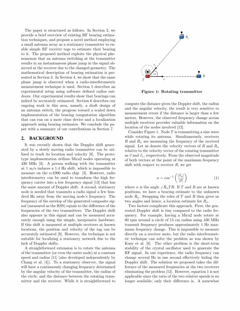
Figure 1: Rotating transmitter

compute the distance given the Doppler shift, the radiusand the angular velocity, the result is very sensitive tomeasurement errors if the distance is larger than a fewmeters. However, the observed frequency change acrossmultiple receivers provides valuable information on thelocation of the nodes involved [12].

Consider Figure 1. Node T is transmitting a sine wavewhile rotating its antenna. Simultaneously, receiversR and Rx are measuring the frequency of the receivedsignal. Let us denote the velocity vectors of R and Rxrelative to the velocity vector of the rotating transmitteras ~v and ~vx, respectively. From the observed magnitudeof both vectors at the point of the maximum frequencyshift with respect to receiver R, we get

α = cos−1

(|~vx||~v|

)(1)

where α is the angle ∠RxTR. If T and R are at knownpositions, we have a bearing estimate to the unknownnode Rx. Swapping the roles of T and R then gives ustwo angles and hence, a location estimate for Rx.

Two factors complicate this approach. First, the gen-erated Doppler shift is tiny compared to the radio fre-quency. For example, having a Mica2 node rotate at60 rpm around a circle of 15 cm radius using 430 MHztransmit frequency produces approximately 1 Hz max-imum frequency change. This is impossible to measuredirectly on a receiver mote, but the radio interferomet-ric technique can solve the problem as was shown byKusy et al. [8]. The other problem is the short-termstability of the crystal oscillator used to generate theRF signal. In our experience, the radio frequency canchange several Hz in one second effectively hiding theDoppler shift. The solution we proposed takes the dif-ference of the measured frequencies at the two receiverseliminating the problem [12]. However, equation 1 is notapplicable since the ratio of the two relative speeds is nolonger available; only their difference is. A somewhat

more complicated approximate solution still producesgood bearing estimates [12].

A corresponding application scenario would utilize 3or more anchor nodes typically surrounding an areawhere statically deployed and/or mobile RF tags (e.g.wireless sensor nodes) are located. The anchor nodesrotate their antennas one by one according to a sched-ule and the RF tags and the remaining anchor nodesmeasure the generated Doppler shift. Then the anchornodes broadcast their own measurements and positionsto the network and in turn, each node would computeits own location. The whole procedure would take acouple of minutes.

This scenario is indeed feasible, but has a significantdrawback. The need to rotate the antennas or nodesmakes the setup more complicated, more power hungry,more expensive and less robust. These are exactly thedesign parameters that one tries to optimize in wirelesssensor network applications, for example. How can weeliminate the rotation from this scenario?

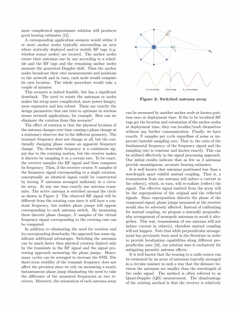
The effect of rotation is that the physical location ofthe antenna changes over time causing a phase change ata stationary observer due to the different geometry. Thetransmit frequency does not change at all, but the con-tinually changing phase causes an apparent frequencychange. The observable frequency is a continuous sig-nal due to the rotating motion, but the receiver makesit discrete by sampling it at a certain rate. To be exact,the receiver samples the RF signal and then computesits frequency. Then, if the receiver creates N samples ofthe frequency signal corresponding to a single rotation,conceptually an identical signal could be constructedby having N antennas arranged uniformly in a circu-lar array. At any one time exactly one antenna trans-mits. The active antenna is switched around the circleas shown in Figure 2. The observed RF signal will bedifferent from the rotating case since it will have a con-stant frequency, but sudden phase jumps will appearcorresponding to each antenna switch. By measuringthese discrete phase changes, N samples of the virtualfrequency signal corresponding to the rotating case canbe computed.

In addition to eliminating the need for rotation andits corresponding drawbacks, the approach has some sig-nificant additional advantages. Switching the antennascan be much faster then physical rotation limited onlyby the transients in the RF signal and the signal pro-cessing approach measuring the phase jumps. Hence,many cycles can be averaged to increase the SNR. Theshort-term stability of the transmit frequency does notaffect the precision since we rely on measuring a nearlyinstantaneous phase jump eliminating the need to takethe difference of the measured frequencies at two re-ceivers. Moreover, the orientation of each antenna array

Ai+1

AR

Ai

Copyright © 2004-2008, Vanderbilt University

Phase change Ai+1 is transmittingAi is transmitting

Figure 2: Switched antenna array

can be measured by another anchor node at known posi-tion once at deployment time. If the to be localized RFtags get the location and orientation of the anchor nodesat deployment time, they can localize/track themselveswithout any further communication. Finally, we haveexactly N samples per cycle regardless of noise or im-precise/instable sampling rate. That is, the ratio of thefundamental frequency of the frequency signal and thesampling rate is constant and known exactly. This canbe utilized effectively in the signal processing approach.Our initial results indicate that as few as 3 antennasprovide unambiguous, accurate bearing estimates.

It is well known that antennas positioned less than awavelength apart exhibit mutual coupling. That is, atransmission from one antenna will induce a current inthe other(s), which, in turn, will re-radiate (reflect) thesignal. The effective signal emitted from the array willbe the superposition of the original and the reflectedsignals. Since superposition distorts the phase of thecompound signal, phase jumps measured at the receiverwould also be adversely affected. Instead of calibratingfor mutual coupling, we propose a mutually perpendic-ular arrangement of monopole antennas to avoid it alto-gether. This way, transmission of one antenna will notinduce current in other(s), therefore mutual couplingwill not happen. Note that while perpendicular arrange-ment has previously been used in the literature in orderto provide localization capabilities along different per-pendicular axes [16], our solution uses it exclusively formitigating parasitic antenna effects.

It is well known that the bearing to a radio source canbe estimated by an array of antennas typically arrangedin a circular manner in such a way that the distance be-tween the antennas are smaller than the wavelength ofthe radio signal. The method is often referred to asQuasi-Doppler (QD) measurement. The disadvantageof the existing method is that the receiver is relatively

large because of the multiple antennas (typically 8 or16). Also, it is computationally intensive the process thehigh frequency radio signals especially since it needs tobe done on all channels simultaneously. Thus, it cannotbe done on small, inexpensive radio tags. Our approachturns the traditional Quasi-Doppler technique aroundutilizing the antenna array on the transmitter side. Thismakes it possible to obtain bearing information using asingle antenna. When augmented with the radio in-terferometric technique, the low frequency beat signal(with instantaneous phase jumps) can be observed withmote class devices.

The approach is somewhat similar to the aircraft radionavigation system, VHF Omni-directional Radio Range(VOR) developed in the 1960s and still being used to-day [1]. The VOR system uses two 30 Hz signals: afrequency modulated omnidirectional reference signaland a rotating directional signal (originally mechani-cally rotated, but today using an antenna array) whichis perceived as an amplitude modulated signal at the re-ceiver. A variant of the system uses the Doppler effectand applies 50 antennas for the variable phase. Whilethe purpose of VOR is the same, to provide bearinginformation by transmitting a radio signal using an an-tenna array, the similarities end there. Our techniquetransmits an unmodulated fixed frequency signal contin-uously switching the single active antenna around andthere is no reference signal. Furthermore, we rely onradio interferometry to enable very simple, low cost andexisting COTS hardware to derive bearing information.

3. BEARING ESTIMATIONThe rate of change of the phase of a signal is its fun-

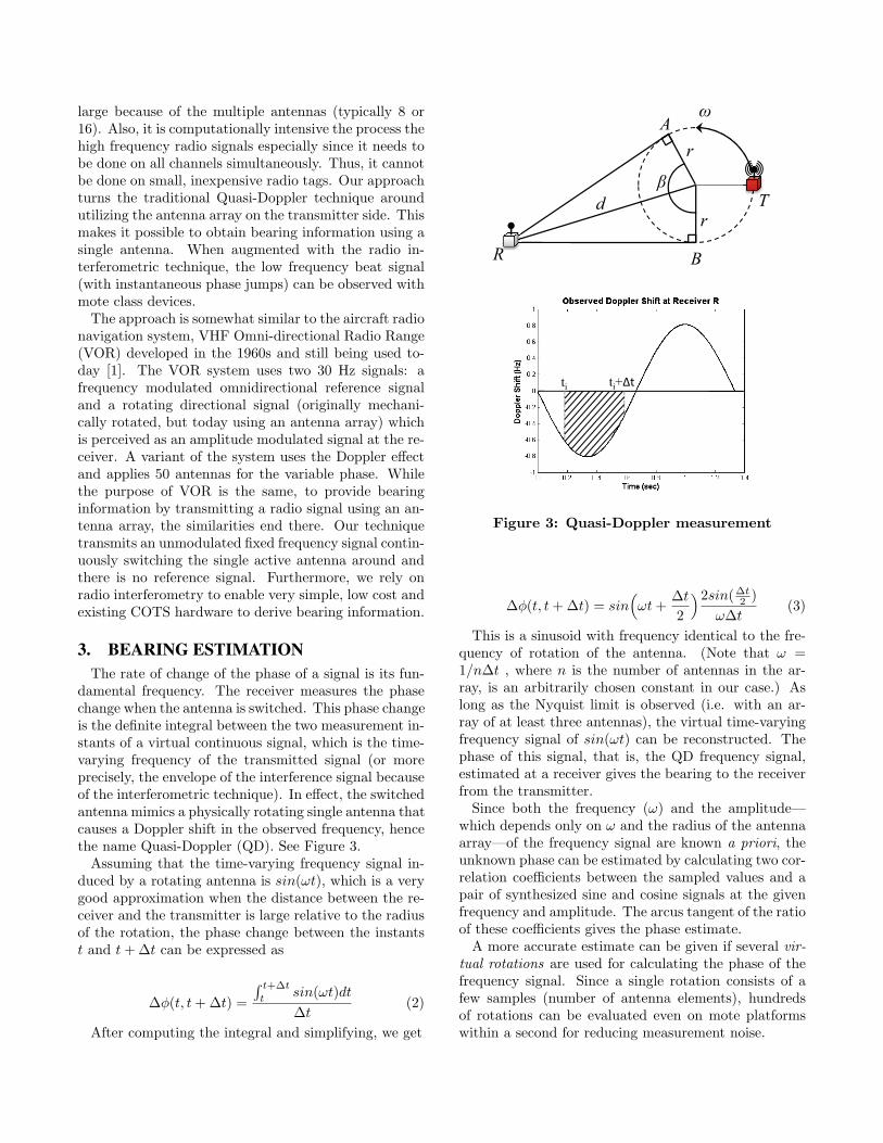
damental frequency. The receiver measures the phasechange when the antenna is switched. This phase changeis the definite integral between the two measurement in-stants of a virtual continuous signal, which is the time-varying frequency of the transmitted signal (or moreprecisely, the envelope of the interference signal becauseof the interferometric technique). In effect, the switchedantenna mimics a physically rotating single antenna thatcauses a Doppler shift in the observed frequency, hencethe name Quasi-Doppler (QD). See Figure 3.

Assuming that the time-varying frequency signal in-duced by a rotating antenna is sin(ωt), which is a verygood approximation when the distance between the re-ceiver and the transmitter is large relative to the radiusof the rotation, the phase change between the instantst and t+ ∆t can be expressed as

∆φ(t, t+ ∆t) =

∫ t+∆t

tsin(ωt)dt∆t

(2)

After computing the integral and simplifying, we get

Ar

ω

β

rd

R

T

BR

ti ti+Δt

Copyright © 2004-2008, Vanderbilt University

Figure 3: Quasi-Doppler measurement

∆φ(t, t+ ∆t) = sin(ωt+

∆t2

)2sin(∆t2 )

ω∆t(3)

This is a sinusoid with frequency identical to the fre-quency of rotation of the antenna. (Note that ω =1/n∆t , where n is the number of antennas in the ar-ray, is an arbitrarily chosen constant in our case.) Aslong as the Nyquist limit is observed (i.e. with an ar-ray of at least three antennas), the virtual time-varyingfrequency signal of sin(ωt) can be reconstructed. Thephase of this signal, that is, the QD frequency signal,estimated at a receiver gives the bearing to the receiverfrom the transmitter.

Since both the frequency (ω) and the amplitude—which depends only on ω and the radius of the antennaarray—of the frequency signal are known a priori, theunknown phase can be estimated by calculating two cor-relation coefficients between the sampled values and apair of synthesized sine and cosine signals at the givenfrequency and amplitude. The arcus tangent of the ratioof these coefficients gives the phase estimate.

A more accurate estimate can be given if several vir-tual rotations are used for calculating the phase of thefrequency signal. Since a single rotation consists of afew samples (number of antenna elements), hundredsof rotations can be evaluated even on mote platformswithin a second for reducing measurement noise.

4. RADIO INTERFEROMETRYSince processing high frequency signals on low-power

COTS wireless nodes is not feasible, we use a radio-interferometric technique originally introduced by Marotiet al. [13] that allows for measuring the phase shift byanalyzing a low frequency beat signal. In addition to theantenna array transmitting a sinusoid of frequency f , anarbitrarily positioned auxiliary antenna is transmittinga sinusoid of frequency f − fi. The superposition ofthe two signals generates an interference field with beatfrequency fi. Setting the interference frequency to fi< 1kHz makes it possible to analyze the signal withresource-constrained wireless nodes.

Below we show that a phase change in the high fre-quency sinusoid results in an equivalent phase change inthe beat signal based on the discussion in [13]. We as-sume that the receiver observes the low-frequency beat-ing using the the received signal strength indicator (RSSI)signal provided by the RF transceiver chip. We modelthe RSSI signal as the power of the incoming signalmixed down to an intermediate frequency fIF , whichgoes through a low-pass filter with cut-off frequencyfcut, where fcut << fIF . Let us assume that the re-ceiver is observing s(t), the superposition of a sinusoidof frequency f , amplitude a1 and phase ϕ1 originatingfrom the transmitter array and a sinusoid of frequencyf − fi, amplitude a2 and phase ϕ2 from the auxiliarytransmitter:

s(t) = a1cos(2πft+ ϕ1) + a2cos(2π(f − fi)t+ ϕ2)

Maroti et al [13] presented the steps to obtain theRSSI signal, which is a sinusoid of frequency 2δ, with aD/C offset:

sRSSI(t) =a2

1 + a22

2+ a1a2cos(4πδt+ ϕ1 − ϕ2)

From here, it is obvious that when the phase of ei-ther high frequency sinusoid component changes, thesame amount of phase change will be observed in theobserved low-frequency beat signal. Since in our sce-nario, the phase of the signal originating from the aux-iliary transmitter does not change, a phase change in thehigh-frequency signal from the antenna array will resultin an equivalent phase change in the beat signal, ob-served using the RF transceiver chip’s RSSI circuitry.

5. EXPERIMENTAL EVALUATIONWe conducted an experiment to verify that the the-

ory does translate to practice, and that it is possible tomeasure the instantaneous phase jumps correspondingto antenna switchings in a reasonably simple way (i.e.the algorithm can scale down to mote-class hardware).

Also, we intended to discover the magnitude and ef-fects of measurement noise, and the limitations the noiseposes on the feasibility and precision of bearing estima-tion. Finally, we used the experimental results to infersome properties of a proposed switched antenna arraydesign (number and arrangement of antennas, switch-ing patterns, etc.) that allows for minimizing non-idealantenna effects and for mitigating bearing estimationerrors resulting from measurement noise.

To minimize environmental disturbances, the experi-ment was conducted outdoors in an open, rural area.

5.1 Setup

5.1.1 Radio hardwareAlthough the proposed idea can be implemented on

resource constrained devices and does not contain com-putational intensive algorithms, we made the first ex-periments with a software defined radio (SDR) platform,the GNU Radio [7]. The use of GNU Radio and the Uni-versal Software Radio Peripheral (USRP) [5] enabledus to generate and/or capture raw radio signals with abandwidth of up to 8 MHz. This platform also provideda highly flexible framework for experimenting with dif-ferent signal processing techniques. Furthermore, theUSRP frontend provides two (simultaneous) transmitand receive paths, thus simple experiments with a two-antenna array could be made without building an actualantenna switch.

FREQSYNTH

CLKREF

FREQSYNTH

RF FRONTEND

SIDE A SIDE B

RF FRONTEND

64 MHz

USRP

FPGA

μC

PC / GNU Radio

DAC

USB (data / control)

A B

data control

controldata

0 2000 4000 6000 8000 10000 12000-1

-0.8

-0.6

-0.4

-0.2

0

0.2

0.4

0.6

0.8

1

DAC

0 2000 4000 6000 8000 10000 12000-1

-0.8

-0.6

-0.4

-0.2

0

0.2

0.4

0.6

0.8

1

0 2000 4000 6000 8000 10000-1

-0.8

-0.6

-0.4

-0.2

0

0.2

0.4

0.6

0.8

1

0 2000 4000 6000 8000 10000-1

-0.8

-0.6

-0.4

-0.2

0

0.2

0.4

0.6

0.8

1

0 2000 4000 6000 8000 10000 12000-1

-0.8

-0.6

-0.4

-0.2

0

0.2

0.4

0.6

0.8

1

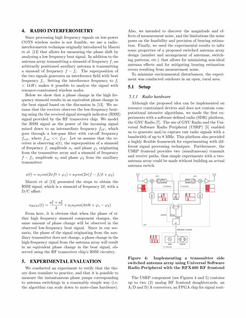
Figure 4: Implementing a transmitter sideswitched antenna array using Universal SoftwareRadio Peripheral with the RFX400 RF frontend

The USRP component (see Figures 4 and 5) containsup to two (2) analog RF frontend daughtercards, anA/D and D/A converters, an FPGA chip for signal rout-

ing and signal preprocessing and a high speed USB in-terface controller. Different daughtercards in variousfrequency bands are supported. We used the RFX400frontend, which is capable of transmitting and/or re-ceiving quadrature signals in the 400-500 MHz band.These cards are driven by the same reference clock (64MHz) from the USRP motherboard and synthesize theanalog mixer frequency using a fractional PLL with astep size of 4 MHz. The frontends also contain RF am-plifiers (LNA, IF filter) and TX/RX switches.

The USRP motherboard contains two CODEC chips—one for each RF frontend—with integrated A/D (64MSPS, 12 bits) and D/A (128 MSPS, 14 bits) convert-ers. The transmit path of the CODECs also containdigital upconverters driven by fine tuned numerically-controlled oscillators (NCO). These upconverters (upto 32MHz, 2Hz resolution) are used to ”augment” thecoarse grained tuning of the analog RF frontend boards.Since the CODECs do not provide similar capabilitieson the receive path, the on-board FPGA contains digitaldownconverter cores and decimation filters. The FPGAalso contains (de)interleaving logic and a run-time con-figurable mux/demux pair for routing the logical USBchannels to/from the RF frontends.

The transmit and receive channels are interleaved andtransferred from and to the PC via the USB interfacewith an effective bandwidth of 32MB/s. Most of thesignal processing is done on the PC using GNU Radio,a generic signal processing framework and a rich set ofcommon signal processing blocks. The blocks are im-plemented in C++, but the configuration of the signalpath is defined in Python scripts. This provides a highlyefficient and very flexible environment. The dataflowgraph can be (re)configured quite easily using the script-ing language, but after the dataflow started, the actualsignal processing is carried out by pure C/C++ code.

5.1.2 TransmitterFor experimenting with a switched antenna transmit-

ter, we used two identical daughtercards connected tothe same USRP box (Figure 4). The PC side (base-band) synthesized a constant signal with a positive DCoffset and periodically reconfigured the signal routinglogic (mux) on the FPGA between the two RF fron-tends. This constant baseband signal creates an un-modulated carrier at the output of the mixer. Sincethe daughtercards and CODECs are driven by the samereference clock, the two alternative transmit paths usethe exact same frequency for mixing. However, the ini-tial phase of the digital upconverters in the CODECsand of the PLLs on the daugthercards are random andcannot be set, thus we had to manually calibrate forapproximately zero phase offset at the antennas usingan oscilloscope.

Note that for this experiment, we did not use radiointerferometry. Since the SDR platform is flexible andpowerful enough to carry out the signal processing onthe receiver side using the high frequency signal directly,we opted for keeping the setup as simple as possible.Since we experimentally verified the radio inteferomet-ric technique many times in the past under differentscenarios [13], [9], [8], we do not expect any unforseeneffects when we combine it with the Quasi Doppler tech-nique.

0°90°

LNA

0°90°

FREQSYNTH

IF GAIN LPF

ADC

ADC

DDC/ M

RF FRONTEND USRP

2MS/s64MS/s

I

Q

USB

SOFTWARE

FREQSYNTH

0°90°

∑

∑

atanphase

estimate(before/

after)ZC CODER

frequencyestimate

phase jump detector

USB

I

Q

2MS/s

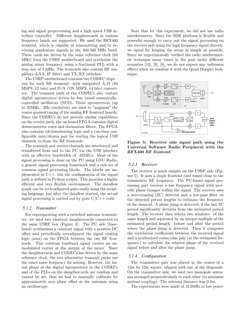
Figure 5: Receiver side signal path using theUniversal Software Radio Peripheral with theRFX400 RF frontend

5.1.3 ReceiverThe receiver is much simpler on the USRP side (Fig-

ure 5). It uses a single frontend card tuned close to thetransmitter RF frequency. The PC-based signal pro-cessing part receives a low frequency signal with peri-odic phase changes within the signal. The receiver usesa zero-crossing (ZC) detector and a low-pass filter onthe detected period lengths to estimate the frequencyof the sinusoid. A phase jump is detected, if the last ZCperiod significantly deviates from the estimated periodlength. The receiver then selects two windows—of thesame length and separated by an integer multiple of theestimated period length—before and after the periodwhere the phase jump is detected. Then it computesthe correlation coefficients between the received signaland a synthesized cosine/sine pair (at the estimated fre-quency) to calculate the relative phase of the receivedsignal before and after the phase jump.

5.1.4 ConfigurationThe transmitter pair was placed in the center of a

12m by 12m square, aligned with one of the diagonals.On the transmitter side, we used two monopole anten-nas arranged perpendicularly to each other (to minimizemutual coupling). The antenna distance was 0.4m.

The experiments were made at 413MHz at low power

levels (few milliwatts). The antenna array was set upto transmit an unmodulated sinusoid at this nominalfrequency. However, the real frequency could deviatefrom this by up to ±50ppm (frequency stability of thereference oscillator). The antenna switching frequencywas set to 50Hz.

The receiver, also an USRP device, equipped with asingle antenna, was used to measure the phase jumpsresulting from antenna switchings at multiple surveyedpoints on the square. The surveyed points were the ver-tices, half points and quarter points of the sides of thesquare. The surveyed points can be seen at angles 0,18.5, 45, 71.5, 90, 108.5, .., -45, -18.5 degrees, respec-tively.

The receiver was tuned to receive at 413.001MHz.This means that the RF input received through theantenna is effectively multiplied by a 413.001MHz sinu-soid, and is then lowpass filtered with a cutoff frequencyof 32MHz. As a result, we expected to see a 1kHz si-nusoid as the received signal. The USRP receiver wasprogrammed to sample at 2MHz.

5.2 Results

5.2.1 Phase jump detectionThe measured periods were typically 950 to 1050 sam-

ples long, which corresponds to a received frequency of2105Hz to 1904Hz at a sampling rate of 2MHz. We ob-served that the mean period length is slowly changingwith time, and the measured period length has a jitterbetween ±5 samples (±0.5% )in the short term. Thiscan be attributed to two phenomena:

• Frequency difference of local oscillators from thenominal frequency. The real crystal frequency most-ly depends on temperature and changes slowly withtime. Since both the transmitter and the receiverwere operating under similar environmental condi-tions, the observed signal frequency differed onlyby 1kHz from the expected. As the phase jump de-tection algorithm uses just a short window of ±10periods centered around the phase jump, it wassafe to assume the period length to be constant.

• Measurement noise. There is an additive measure-ment noise on the received signal, which causesthe measured period lengths to fluctuate between±5 samples around the short-term mean periodlength. As a result, phase jumps that are equiva-lent or smaller in magnitude that the noise-relatedjitter in period length are not possible to detect.Hence, the phase jump detection algorithm hasblind spots around bearings of 90 and -90 degrees,where the expected phase jump is close to zero.

0 1000 2000 3000 4000 5000−3000

−2000

−1000

0

1000

2000

3000

samples

ampl

itude

An instantaneous phase jump in received signal

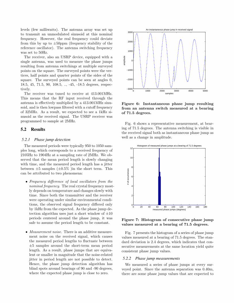
Figure 6: Instantaneous phase jump resultingfrom an antenna switch measured at a bearingof 71.5 degrees.

Fig. 6 shows a representative measurement, at bear-ing of 71.5 degrees. The antenna switching is visible inthe received signal both as instantaneous phase jump aswell as a change in amplitude.

0 20 40 60 80 100 120 140 160 1800

2

4

6

8

10

12

measured phase jumps (degrees)

# of

occ

urre

nces

Histogram of measured phase jumps at a bearing of 71.5 degrees

Figure 7: Histogram of consecutive phase jumpvalues measured at a bearing of 71.5 degrees.

Fig. 7 presents the histogram of a series of phase jumpvalues measured at a bearing of 71.5 degrees. The stan-dard deviation is 2.4 degrees, which indicates that con-secutive measurements at the same location yield quiteconsistent phase jump values.

5.2.2 Phase jump measurementsWe measured a series of phase jumps at every sur-

veyed point. Since the antenna separation was 0.40m,there are some phase jump values that are expected to

−200 −150 −100 −50 0 50 100 150 200−250

−200

−150

−100

−50

0

50

100

150

200Expected vs. measured phase jumps − uncalibrated case

bearing of receiver (degrees)

mea

sure

d ph

ase

jum

p (d

egre

es)

expected phase jumpmeasured phase jump

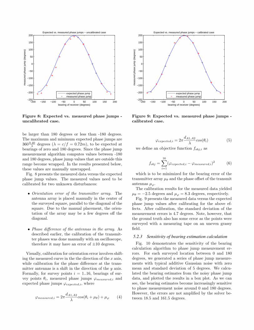
Figure 8: Expected vs. measured phase jumps -uncalibrated case.

be larger than 180 degrees or less than -180 degrees.The maximum and minimum expected phase jumps are360 0.40

λ degrees (λ = c/f = 0.72m), to be expected atbearings of zero and 180 degrees. Since the phase jumpmeasurement algorithm computes values between -180and 180 degrees, phase jump values that are outside thisrange become wrapped. In the results presented below,these values are manually unwrapped.

Fig. 8 presents the measured data versus the expectedphase jump values. The measured values need to becalibrated for two unknown disturbances:

• Orientation error of the transmitter array. Theantenna array is placed manually in the center ofthe surveyed square, parallel to the diagonal of thesquare. Due to the manual placement, the orien-tation of the array may be a few degrees off thediagonal.

• Phase difference of the antennas in the array. Asdescribed earlier, the calibration of the transmit-ter phases was done manually with an oscilloscope,therefore it may have an error of ±10 degrees.

Visually, calibration for orientation error involves shift-ing the measured curve in the the direction of the x axis,while calibration for the phase difference at the trans-mitter antennas is a shift in the direction of the y axis.Formally, for survey points i = 1..16, bearings of sur-vey points θi, measured phase jumps ϕmeasured,i andexpected phase jumps ϕexpected,i, where

ϕmeasured,i = 2πdA1,A2

λcos(θi + µθ) + µϕ (4)

−200 −150 −100 −50 0 50 100 150 200−250

−200

−150

−100

−50

0

50

100

150

200Expected vs. measured phase jumps − calibrated case

bearing of receiver (degrees)

mea

sure

d ph

ase

jum

p (d

egre

es)

expected phase jumpmeasured phase jump

Figure 9: Expected vs. measured phase jumps -calibrated case.

ϕexpected,i = 2πdA1,A2

λcos(θi) (5)

we define an objective function fobj,i as

fobj =16∑i=1

(ϕexpected,i − ϕmeasured,i)2 (6)

which is to be minimized for the bearing error of thetransmitter array µθ and the phase offset of the transmitantennas µϕ.

The calibration results for the measured data yieldedµθ = −2.5 degrees and µϕ = 8.3 degrees, respectively.

Fig. 9 presents the measured data versus the expectedphase jump values after calibrating for the above ef-fects. After calibration, the standard deviation of themeasurement errors is 4.7 degrees. Note, however, thatthe ground truth also has some error as the points weresurveyed with a measuring tape on an uneven grassyfield.

5.2.3 Sensitivity of bearing estimation calculationFig. 10 demonstrates the sensitivity of the bearing

calculation algorithm to phase jump measurement er-rors. For each surveyed location between 0 and 180degrees, we generated a series of phase jump measure-ments with typical additive Gaussian noise with zeromean and standard deviation of 5 degrees. We calcu-lated the bearing estimates from the noisy phase jumpdata, and plotted the results in a box plot. As we cansee, the bearing estimates become increasingly sensitiveto phase measurement noise around 0 and 180 degrees.However, the errors are not amplified by the solver be-tween 18.5 and 161.5 degrees.

0 18.5 45 71.5 90 108.5 135 161.5 180

−10

−5

0

5

10

abso

lute

bea

ring

estim

atio

n er

ror

(deg

rees

)

bearing of receiver (degrees)

Sensitivity of bearing estimation error to phase jump measurement errors

Figure 10: Sensitivity of bearing estimation tophase measurement error

5.3 EvaluationBased on the experimental results, we can draw the

following conclusions:

• Measurement of instantaneous phase jumps result-ing from antenna switchings is feasible. The aboveexperimental results show that it is possible tomeasure phase jumps resulting from the alterna-tion of transmit antennas unless the phase jumpis less than the phase jitter due to measurementnoise, which happens at bearings around 90 and-90 degrees.

• Phase jump detection and computation scales downto wireless sensor node class devices. While theabove measurements were taken with highly so-phisticated radio hardware, this approach can scaledown to simple devices with limited processing ca-pabilities.

• No significant nonideal antenna effects. With theexperimental two-antenna array we could not iden-tify any nonideal antenna effects.

• Bearing estimation from phase jump measurementsis feasible. We have verified that it is possible toestimate the bearing of a receiver with respect toan antenna array given the assumptions outlinedin Section 3. We have observed, however, that atbearings around 0 and 180 degrees, the errors ofthe bearing estimation are very sensitive to errorsin phase jump measurements.

Based on the above findings, an antenna array shouldhave the following properties to be suitable for bearingestimation:

• Antenna separation. Distance between antennasbetween which switchings will occur must be lessthan λ/2, where λ is the wavelength of the fre-quency of the RF signal, in order to avoid wrap-ping around of phase jump measurements.

• Spatial diversity of antenna arrangement. Bearingestimates around ±90 degrees, as well as around0 and 180 degrees should be discarded, because ofthe blind spots of the phase jump measurementand the oversensitivity of the bearing estimationcalculation algorithm, respectively. Ideally, theantenna arrangement should be such that if thereceiver is in the blind spot/oversensitive regionof a pair of antennas, there is at least two otherpairs of antennas for which the receiver is outsideof their blind spots/oversensitive regions. That is,antenna pairs that lie on lines that are perpen-dicular should be avoided, since the blind spot ofone pair will coincide with the oversensitive regionof the other pair, and vice versa. Furthermore, an-tenna pairs that lie on lines that are parallel shouldalso be avoided, since their blind spots, as well astheir oversensitive regions, will coincide. A circu-lar antenna array with an odd number of elementswill not suffer from these deficiencies, however, andthus it is a safe choice for our technique.

6. WORK IN PROGRESSThis section highlights three research directions that

we are actively working on at the time of publishing ofthis paper. Our primary goal is to replace the heavy-weight software defined radio equipment on both thetransmitter and the receiver side with low-power mote-class devices. We envision an asymmetric architecturewhere the stationary transmitter nodes are equippedwith an antenna switch, while the mobile receivers haveonly single antennas. Below, we present a preliminarydesign draft of an antenna switch that can be connectedto a Mica2 mote. Then, we present the challenges andcurrent status of scaling down the signal processing tasksdescribed in Section 5 to mote class devices. Finally, weprovide a brief description on how we envision usingbearing estimates for node localization.

6.1 Antenna switch designOur USRP-based experimental setup for the switched

antenna transmitter (see Section 5) enabled two anten-nas only and added unnecessary complexity to the trans-mitter side (two complete transmitter frontends insteadof just two antennas). For these reasons, having a moresuitable transmitter platform is critical in the futuredevelopment of the presented approach. In the follow-ing section, we outline the most important requirements

and potential pitfalls for a switched antenna array to beused for Radio Interferometric Quasi Doppler BearingEstimation. The block diagram of the antenna switchboard we are planning to build is shown in Figure 11.

The antenna switch should completely decouple theswitching logic from the transmitter radio (to be able touse the device with almost any RF transmitter). Also,the board should be able to switch between the an-tennas using arbitrary sequence and timing patterns(e.g., encoding information in the switch time inter-vals). Thus, the core functionality of the board is imple-mented by an on-board microcontroller controlling theRF switch/demultiplexer component.

0°90°

SP4T(absorptive)

SPST(reective)

μCMOTE

CONNECTOR(s)

DC/DC CONVERTER

REF CLOCK

DDS PLL

SIGNAL GENERATOR

RF in

RF1 out

RF2 out

RF3 out

RF4 out

RF out

RF SWITCHES

Figure 11: Block diagram of the proposed au-tonomous antenna switch board

Two prevalent technologies are used to implement thenonlinear element of an RF switch: in PIN diodes, thebias DC current controls the impedance of the diode atRF frequencies, whereas in GaAs FETs, the transistor isfully ”on” or ”off” depending upon the bias conditions).While PIN diodes are more tolerant against high powerRF pulses, GaAs switches offer faster switching time andRF response extending down to DC. For these reasons,GaAs FETs are more suitable in the proposed applica-tion. Another important design choice is the termina-tion of the ports in the ”off”state. Reflective switch out-puts either appear as short or open circuits to the con-nected antenna element resulting in a very high VSWR(reflection ratio). Absorptive switches present 50 Ωimpedance on all outputs/inputs regardless of the switchstate. The primary goal when selecting the switch topol-ogy in the proposed application is to minimize the effectof the passive (parasitic) antenna elements on the activeantenna. Optionally, the performance of the antenna

array can be improved by controlling the impedance ofthe parasitic elements, thereby steering the radiationpattern [18, 15]. To achieve these goals we propose twolayers of switches: the initial switch (SP4T or SP8T)being an absorptive component with dedicated SPSTreflective switches added to each output. Using thistopology one can experiment with and minimize theeffects of the different impedance alternatives for theparasitic elements. Due to the bi-directionality of theswitch components, the antenna switch board can beused both on the transmitter and/or the receiver sides.

The antenna elements should be connected to theboard through flexible coaxial cables to be able to ex-periment with various antenna spacing and layouts andto keep the size of the board relatively small. For thevery same reason, a self-contained power supply solutionis preferred. The power requirements of the board aremoderate (<10mA @ 3V), a pair of AA-size batterieswith a DC/DC converter (3.3V, 5V) is sufficient.

Connectors for existing mote platforms (Mica2, Mi-caZ, IRIS, Telos ) can provide communication channels(I2C, UART) to the on-board microcontroller (e.g., timesynchronization between the boards, high-level controlinterface). They can also provide (consume) power to(from) the connected mote.

Finally, an on-board frequency synthesizer could trans-form the antenna switching board to a self-containedtransmitter node in the proposed application. Martinidescribes a novel and low-cost approach to implementa highly tunable (200 Hz resolution) wide-band signalgenerator with low phase noise by utilizing a DDS com-ponent as the reference clock for the PLL section of thetransceiver [14].

6.2 Receiver implementationScaling down the signal processing algorithm that com-

putes the magnitude of the phase jumps observed at thereceiver to run on mote class hardware is a challeng-ing task. In our previous work on radio-interferometrictracking [9] we had shown that sampling the RSSI at8kHz (8-bit samples) is feasible using the Mica2 mote,which leaves approximately 800 clock cycles for process-ing per each sample. This implies that all processingmust be done using fixed point arithmetics in the timedomain, and excessive use of multiply-and-sum opera-tions (e.g. long FIR filters) should be avoided.

We are currently experimenting with the following al-gorithm. First, we remove high-frequency noise fromthe raw RSSI readings with a moving averager (whichis, effectively, a low-pass filter). Keeping a history ofsamples in a circular buffer, a moving averager can beinexpensively implemented by maintaining an accumu-lator variable that contains the sum of the samples inthe buffer. If the history size is a power of two, the

output of the moving averager can be computed withbitwise shifting of the accumulator, instead of the moreexpensive integer division.

A switch from one transmit antenna to another, be-side resulting in an instantaneous phase jump at thereceiver, may also changes the amplitude and the D/Coffset of the RSSI signal. To remove the D/C offset,we use a derivator followed by a leaky integrator, whichis common practice in digital signal processing. Thederivator is essentially a two-tap FIR filter, such thaty[n] = x[n]−x[n− 1], while the integrator is a one-poleIIR filter, such that y[n] = α ∗ y[n − 1] + x[n], where0 < α < 1 is the pole. This can be implemented withbitwise shifts instead of multiplication if we choose thepole such that α = (2n−1)/2n. Also, to mitigate quanti-zation errors, we represent the integrator’s accumulatoron 32 bits instead of 8 bits.

Once the D/C offset is removed, we use a simplezero-crossing decoder to find the period lengths, i.e.the sample distance between consecutive negative-to-positive transitions. We store the the period lengthsin a buffer.

When the buffer is full, we stop sampling the RSSIand start a task that processes the period lengths of-fline. Currently, the offline task is searching for sharpchanges in period lengths, which indicate an observedphase jump in the received signal. Precisely, 2π timesthe ratio of the outlier period length and the precedingnormal period length gives magnitude of phase jump.From here, we use Equation 5 to compute the bearing.

As of writing this paper, this algorithm performs wellon simulated data but falls short in precision when run-ning on noisy RSSI readings acquired by the Mica2motes. Currently, we are investigating how mitigatingmeasurement noise would be possible with simple signalprocessing algorithms on mote class devices.

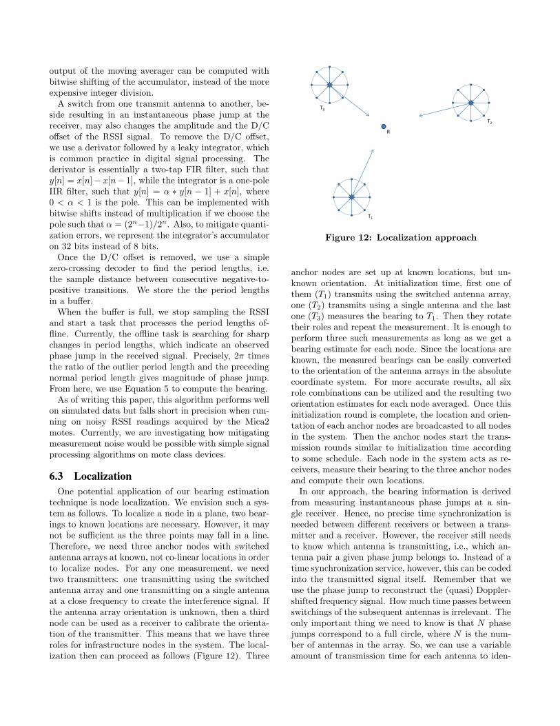
6.3 LocalizationOne potential application of our bearing estimation

technique is node localization. We envision such a sys-tem as follows. To localize a node in a plane, two bear-ings to known locations are necessary. However, it maynot be sufficient as the three points may fall in a line.Therefore, we need three anchor nodes with switchedantenna arrays at known, not co-linear locations in orderto localize nodes. For any one measurement, we needtwo transmitters: one transmitting using the switchedantenna array and one transmitting on a single antennaat a close frequency to create the interference signal. Ifthe antenna array orientation is unknown, then a thirdnode can be used as a receiver to calibrate the orienta-tion of the transmitter. This means that we have threeroles for infrastructure nodes in the system. The local-ization then can proceed as follows (Figure 12). Three

T3

R

T2

Copyright © 2004-2008, Vanderbilt University

T1

Figure 12: Localization approach

anchor nodes are set up at known locations, but un-known orientation. At initialization time, first one ofthem (T1) transmits using the switched antenna array,one (T2) transmits using a single antenna and the lastone (T3) measures the bearing to T1. Then they rotatetheir roles and repeat the measurement. It is enough toperform three such measurements as long as we get abearing estimate for each node. Since the locations areknown, the measured bearings can be easily convertedto the orientation of the antenna arrays in the absolutecoordinate system. For more accurate results, all sixrole combinations can be utilized and the resulting twoorientation estimates for each node averaged. Once thisinitialization round is complete, the location and orien-tation of each anchor nodes are broadcasted to all nodesin the system. Then the anchor nodes start the trans-mission rounds similar to initialization time accordingto some schedule. Each node in the system acts as re-ceivers, measure their bearing to the three anchor nodesand compute their own locations.

In our approach, the bearing information is derivedfrom measuring instantaneous phase jumps at a sin-gle receiver. Hence, no precise time synchronization isneeded between different receivers or between a trans-mitter and a receiver. However, the receiver still needsto know which antenna is transmitting, i.e., which an-tenna pair a given phase jump belongs to. Instead of atime synchronization service, however, this can be codedinto the transmitted signal itself. Remember that weuse the phase jump to reconstruct the (quasi) Doppler-shifted frequency signal. How much time passes betweenswitchings of the subsequent antennas is irrelevant. Theonly important thing we need to know is that N phasejumps correspond to a full circle, where N is the num-ber of antennas in the array. So, we can use a variableamount of transmission time for each antenna to iden-

tify it. If we have multiple antenna arrays, the sametechnique can be used to identify the currently active ar-ray also. The only requirement is that the transmissiontime for each antenna in the system needs to be globallyunique and distinguishable by the receivers given theirclock resolution and accuracy.

7. CONCLUSIONThe paper presented a novel idea for bearing estima-

tion in wireless networks and our preliminary work val-idating it. The unique components of our method are

• Using the switched antenna array on the transmit-ter side as opposed to the receiver side that is tra-ditional in Quasi-Doppler bearing estimation, sothat a single antenna receiver can obtain bearinginformation.• Using our radio interferometric technique to trans-

form the useful phase information from the highfrequency radio signal (typically >100 MHz) to alow frequency signal (< 1 kHz) that can be pro-cessed on low-cost hardware.• The antenna array can have as few as 3 antennas

for unambiguous bearing estimation.• The proposed antenna switch design can be either

a plug-in replacement for a traditional antenna fora mote or SDR, for example, or a standalone trans-mitter in and of itself.

While there exist challenges before a successful imple-mentation of a full-scale localization service relying onour method will be achieved, the initial results are verypromising.

8. REFERENCES[1] 2001 Federal Radionavigation Systems. http://

www.navcen.uscg.gov/pubs/frp2001/FRS2001.pdf.[2] Pango. http://www.pangonetworks.com, 2008.[3] Chipcon AS, CC1000: Single chip very low power

RF transceiver. http://www.chipcon.com, 2004.[4] H.-L. Chang, J.-B. Tian, T.-T. Lai, H.-H. Chu,

and P. Huang. Spinning beacons for precise indoorlocalization. In Proc. of ACM Sensys, 2008.

[5] Ettus Research LLC. http://www.ettus.com,2008.

[6] R. Fontana, E. Richley, and J. Barney.Commercialization of an ultra wideband precisionasset location system. Ultra Wideband Systemsand Technologies, 2003 IEEE Conference on,pages 369–373, 16-19 Nov. 2003.

[7] GNU Radio website. http://gnuradio.org, 2008.[8] B. Kusy, A. Ledeczi, and X. Koutsoukos. Tracking

mobile nodes using rf doppler shifts. In Proc. ofACM SenSys, 2007.

[9] B. Kusy, J. Sallai, G. Balogh, A. Ledeczi,V. Protopopescu, J. Tolliver, F. DeNap, andM. Parang. Radio interferometric tracking ofmobile wireless nodes. In Proc. of MobiSys, 2007.

[10] Y. Kwon and G. Agha. Passive localization: Largesize sensor network localization based onenvironmental events. In Proc. of IPSN, pages3–14, 2008.

[11] A. Ledeczi, J. Sallai, P. Volgyesi, andR. Thibodeaux. Differential Bearing Estimationfor RF Tags. EURASIP Journal on EmbeddedSystems (in press), 2009.

[12] A. Ledeczi, P. Volgyesi, J. Sallai, andR. Thibodeaux. A novel rf ranging method.Workshop on Intelligent Solutions in EmbeddedSystems (WISES 2008), July 2008.

[13] M. Maroti, B. Kusy, G. Balogh, P. Volgyesi,A. Nadas, K. Molnar, S. Dora, and A. Ledeczi.Radio interferometric geolocation. In Proc. ofACM SenSys, Nov. 2005.

[14] N. Martini. DIY signal generation. Circuit Cellar,(219):12–23, October 2008.

[15] S. Preston and D. Thiel. Direction finding using aswitched parasitic antenna array. Antennas andPropagation Society International Symposium,1997. IEEE., 1997 Digest, 2:1024–1027 vol.2, Jul1997.

[16] K. Romer. The lighthouse location system forsmart dust. In MobiSys. USENIX, 2003.

[17] R. Stoleru, P. Vicaire, T. He, and J. A. Stankovic.Stardust: a flexible architecture for passivelocalization in wireless sensor networks. In Proc.of ACM SenSys, 2006.

[18] T. Svantesson and M. Wennstrom. High-resolutiondirection finding using a switched parasiticantenna. Statistical Signal Processing, 2001.Proceedings of the 11th IEEE Signal ProcessingWorkshop on, pages 508–511, 2001.

[19] D. Taubenheim, S. Kyperountas, and N. Correal.Distributed radiolocation hardware core for ieee802.15.4. Technical report, Motorola Labs,Plantation, Florida, 2005.

[20] D. Young, C. Keller, D. Bliss, and K. Forsythe.Ultra-wideband (uwb) transmitter location usingtime difference of arrival (tdoa) techniques.Signals, Systems and Computers, 2003.Conference Record of the Thirty-Seventh AsilomarConference on, 2:1225–1229 Vol.2, 9-12 Nov. 2003.

[21] Z. Zhong and T. He. Msp: multi-sequencepositioning of wireless sensor nodes. In Proc. ofACM SenSys, 2007.