1

Railway Traction

José A. Lozano, Jesús Félez, Juan de Dios Sanz and José M. Mera Universidad Politécnica de Madrid

Spain

1. Introduction

The railway as a means of transport is a very old idea. At its beginnings, it was mainly utilised in the central European mines with different means of traction being applied. But it did not come into general use until the invention of the steam engine. Since the 18th century it has developed faster and faster until in the 21st century it has become the most efficient means of transport for medium distances thanks to the development of High Speed.

The main factors that have driven the enormous development of the railway, as any other

means of transport, have been, and continue to be safety, speed and economy. On top of all

this, as every day passes, its environmental impact is minimum, if not zero. In the case of the

railway, one of the determining factors behind its development was the type of track used,

either because of its gauge or the materials used in its construction. At the start, these were

made of cast iron, but they turned out to be lacking in safety as they easily broke due to their

fragility. Towards the end of the 19th century steel began to be used as it was a less fragile

and much stronger material. Nowadays, plate track is a key element in the development of

High Speed trains making wooden sleepers a thing of the past. The rubber track mountings

which are currently used to support the tracks have led to enormous reductions in vibration

and noise both in the track and the rolling stock. Moreover, each country had a different

track gauge due to strategic reasons of commerce and defence. Today’s global markets leave

no other option but to standardise track gauges or failing that, to produce rolling stock that

can be adapted to the different gauges quickly and automatically.

The birth of the railway is linked to the birth of the steam engine, while the tremendous development of the railway in the 20th century was linked to the electrification of the railway lines. In addition, the diesel locomotive played a very important role because of its autonomy, particularly on those lines where electrification was unviable. The rivalry between these three types of locomotive was long and hard with each competing to see which was the safest, fastest and cheapest. The first electric locomotives appeared in the last third of the 19th century, while the first Diesel locomotive was built at the beginning of the 20th century (Faure, 2004). Diesel locomotives never reached the speeds of electric locomotives; however, the latter require a greater investment in infrastructure to electrify the line. As we all know, it is electric locomotives that are at the forefront of railway traction, while the Diesel locomotive is kept for some very specific uses. The final decade of the 20th century and the first decade of the 21st century were marked by the enormous rise in High Speed due to the huge leaps forward in electric locomotive technology.

www.intechopen.com

Reliability and Safety in Railway 4

After this very brief historical introduction, in this chapter, we will now focus on the

different types of railway traction and their importance in the development of the railway,

with particular reference to safety, speed, economy and environmental impact. The basic aim is

to give a detailed description of how the most generally used traction and engine systems

work in present-day railways. An analysis of the critical or least efficient points of the way

they work will lead us to discover the main criteria for optimising railway traction systems.

This could be a starting point for conducting research and seeking innovations to produce

ever more effective and efficient traction systems. The final part of this work will suggest

and justify some ideas that could be useful for improving the operating efficiency of railway

traction systems.

In order to fulfil the objectives described in the above paragraph, a methodology will be

applied that is based on the consideration of physical models that represent the behaviour of

the railway traction systems under study, taking account of all the processes of

transformation, regulation and use of energy and even being able to recover it. Special

attention is placed on the elements that can lead to losses of energy and efficiency.

Specifically, these models are developed using the Bond-Graph technique. This technique is

widely accepted for its capacity to model dynamic systems that embrace various fields of

science and technology. Modelling is performed systematically in a way that enables all the

dynamic, mechanical, electrical, electromagnetic and thermal phenomena, etc, that may be

involved, to be taken into account. Moreover, this technique has more than proven itself to

be suited to modelling vehicular and rail systems. By taking the corresponding conceptual

models, the Bond-Graph models are generated, and, by means of very mechanical

procedures the behaviour equations of the dynamic systems can be found. By then taking

these behaviour equations or mathematical models, computer applications can be built to

simulate, analyse and validate the behaviour of the developed models.

2. General aspects of railway traction

What really causes the train to accelerate or brake are the adhesion forces that appear in the

wheel-rail contact. For these adhesion forces to appear, tractive or braking effort needs to be

applied to the wheels. This torque must be generated in a motor or braking system that

transforms a certain amount of energy into the required mechanical energy. These three

stages form a general summary of the fundamentals of railway traction. All that needs to be

done is to develop a simple model that looks at the phenomena produced from an energy

point of view, from the moment the energy is captured until it reaches the wheel-rail

contact. As a result of all this, the train accelerates or brakes.

2.1 General traction equation, resistance forces

Railway traction is considered to be one of the main problems of longitudinal rail dynamics (Faure, 2004; Iwnicki, 2006). It is seen as a one-dimensional problem located in the longitudinal direction of the track, governed by the Fundamental Law of Dynamics or Newton’s Second Law, applied in the longitudinal direction of the train’s forward motion:

∑F =M·a (1)

www.intechopen.com

Railway Traction 5

Where the term to the left of the equal sign is the sum of all the forces acting in the longitudinal direction of the train, “M” is the total mass and “a” is the longitudinal acceleration experienced by the train. The sum of forces consists of the tractive or braking effort “Ft” and the passive resistances opposing the forward motion of the train, “ΣFR”, (Fig. 1.-). The tractive or braking effort “Ft”, in a final instance, is the resultant of the longitudinal adhesion forces that appear in the wheel-rail contact zones, either when the train’s motors make the wheels rotate in the direction of forward motion, or when the braking forces act to stop the wheels rotating (in this case, these forces will obviously be negative or counter to the direction of the train’s forward motion).

Fig. 1. Longitudinal train dynamics.

Let us now focus on the passive resistances that are opposing the train’s forward motion, “ΣFR”. These basically consist of five types of forces:

a. Rolling resistances of the wheels. b. Friction between the contacting mechanical elements. c. Aerodynamic resistances to the train’s forward motion. d. Resistances to the train’s forward motion on gradients. e. Resistances to the train’s forward motion on curves.

The phenomena associated with the appearance of the aforementioned resistances to the train’s forward motion are widely known (Andrews, 1986 ; Faure, 2004; Coenraad, 2001 ; Iwnicki, 2006). For this reason, we will simply present one of the most common expressions for modern passenger trains:

∑FR = (266,3+27,7∙V+0,05168∙Vに)+(rg+ 5どどR )∙(L+Q) (2)

Where “V” is the train’s speed in (Km/h), “rg” is the inclination of the gradient as a (o/oo), “R” is the radius of the curve in (m), “L” is the weight of the locomotives in (Tm) and “Q” is the towed weight or the weight of the coaches in (Tm).

As can be seen from equation (2), the resistances to forward motion consist of three components: one constant, another that is linearly dependent on speed and another that depends on the speed squared. Moreover, when the train is running on a curve or a gradient, the final term that is not dependent on speed needs to be added.

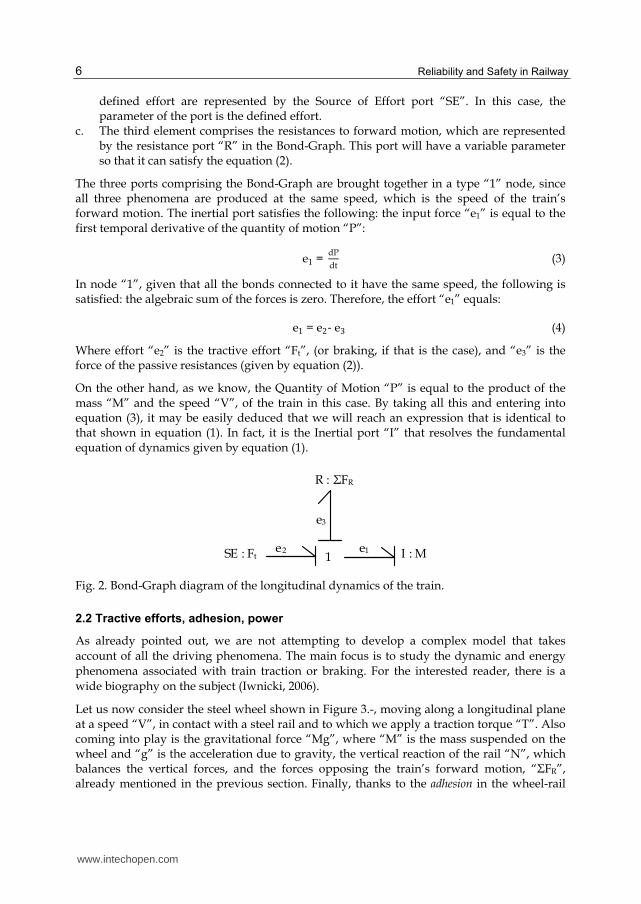
We will now develop the Bond-Graph model, (Karnoppet alia, 2000), for the longitudinal train dynamics expressed in equation (1). In this model, shown in Figure 2, there are three basic elements:

a. The most important element is the train itself, whose longitudinal motion is represented by the Inertial port “I”. The parameter of this port is the train’s total mass, “M”.

b. The tractive or braking efforts “Ft”. In whatever case, this is an element that supplies energy according to a defined force. In Bond-Graphs, these energy sources with a

www.intechopen.com

Reliability and Safety in Railway 6

defined effort are represented by the Source of Effort port “SE”. In this case, the parameter of the port is the defined effort.

c. The third element comprises the resistances to forward motion, which are represented by the resistance port “R” in the Bond-Graph. This port will have a variable parameter so that it can satisfy the equation (2).

The three ports comprising the Bond-Graph are brought together in a type “1” node, since all three phenomena are produced at the same speed, which is the speed of the train’s forward motion. The inertial port satisfies the following: the input force “e1” is equal to the first temporal derivative of the quantity of motion “P”:

e1 = dP

dt (3)

In node “1”, given that all the bonds connected to it have the same speed, the following is satisfied: the algebraic sum of the forces is zero. Therefore, the effort “e1” equals:

e1 = eに- eぬ (4)

Where effort “e2” is the tractive effort “Ft”, (or braking, if that is the case), and “e3” is the force of the passive resistances (given by equation (2)).

On the other hand, as we know, the Quantity of Motion “P” is equal to the product of the mass “M” and the speed “V”, of the train in this case. By taking all this and entering into equation (3), it may be easily deduced that we will reach an expression that is identical to that shown in equation (1). In fact, it is the Inertial port “I” that resolves the fundamental equation of dynamics given by equation (1).

Fig. 2. Bond-Graph diagram of the longitudinal dynamics of the train.

2.2 Tractive efforts, adhesion, power

As already pointed out, we are not attempting to develop a complex model that takes

account of all the driving phenomena. The main focus is to study the dynamic and energy phenomena associated with train traction or braking. For the interested reader, there is a

wide biography on the subject (Iwnicki, 2006).

Let us now consider the steel wheel shown in Figure 3.-, moving along a longitudinal plane at a speed “V”, in contact with a steel rail and to which we apply a traction torque “T”. Also coming into play is the gravitational force “Mg”, where “M” is the mass suspended on the wheel and “g” is the acceleration due to gravity, the vertical reaction of the rail “N”, which balances the vertical forces, and the forces opposing the train’s forward motion, “ΣFR”, already mentioned in the previous section. Finally, thanks to the adhesion in the wheel-rail

e1 e2

e3

I : MSE : Ft 1

R : ΣFR

www.intechopen.com

Railway Traction 7

contact zone, the tangential adhesion force “Ft” appears, which satisfies the following expression:

Ft = μ∙N (5)

Where “µ” is the so-called adhesion coefficient, whose rolling values for wheel and steel rail is dependent on temperature, humidity, dirt, etc, and particularly on speed. An expression that will enable us to find the value of the adhesion coefficient according to speed is the following:

μ=μ搭怠袋待,待怠諾 (6)

Where “V” is the speed of the train in Km/h, and “μo” is the adhesion coefficient for zero speed. The value of “μo” depends on the atmospheric conditions of temperature, humidity, dirt, etc, which under optimum conditions reaches a value of 0’33. Under such conditions and V=300 km/h, we obtain: μ =0.082. Therefore, we can see that the wheel-steel rail contact has limited possibilities when it comes to transmitting the tangential tractive or braking efforts “Ft”,.

Below is the expression used by RENFE in Spain for the adhesion coefficient, where, as is customary, the speed is expressed in km/h:

μ=μ誰 岾ど,になな5 + 戴戴替態袋諾峇 (7)

Fig. 3. Tangential adhesion forces in the wheel-rail contact.

Right from the beginnings of the railway the major challenge of railway traction has been to increase the adhesion coefficient in the wheel-rail contact. Fig. 4 shows some of the adhesion coefficient values “μo”, used. What is surprising is the high value achieved for this coefficient in the United States of America.

www.intechopen.com

Reliability and Safety in Railway 8

Values of “μo”

SNCF (France)

Electric monophase locomotives, multimotor bogies 0.33

Electric monophase locomotives, monomotor bogies 0.35

DB (Germany) Diesel locomotives 0.30

Electric monophase locomotives 0.33

RENFE (Spain)

Diesel locomotives 0.22 - 0.29

Classic electric locomotives 0.27

Modern electric locomotives 0.31

USA SD75MAC diesel and electric locomotives 0.45

Fig. 4. Some values used for “μo”.

Some of the methods used to improve the values of the adhesion coefficient, especially during start up or acceleration, for reasons which will be made clear further on, are:

a. Introduction of sand in the wheel-rail contact. This is the traditional method using devices called “sandboxes”, which are still frequently in use. However, this is a very aggressive system regarding the wear of wheel and rail materials.

b. Monomotor bogies that spread the tractive efforts evenly between all their shafts lead to an optimisation of the adhesion coefficient used.

c. Drawbars that connect the locomotive chassis to the bogies in a way that the locomotive’s weight falls on the lowest part of the bogie at a level that is as close as possible to the wheel-rail contact. Apparently, the accelerations between the locomotive chassis and the bogie generate a force torque that aids the tractive or braking efforts, thus improving wheel-rail adhesion.

d. Electronic anti-slip, braking and traction control systems. These are similar systems to ABS, (Anti-lock Braking System), or ASR, (Anti-Slip Regulation) used in the automotive industry. The speed of the wheels is controlled and regulated by electronic devices so that there is no slip between the wheels and the rails.

In traction, the ideal situation is to have the maximum effort according to speed. As we know, the power developed is the product of force and speed:

Power = F担 ∙ 撃 (8)

Since the power supplied by the motor is approximately constant, the tractive effort available “Ft”, (given by equation (8)), dependent on the train’s speed “V”, complies with a hyperbolic-type ratio, like that shown in Figure 5.

F担 = 牒墜栂勅追蝶 (9)

Apart from the “constant power hyperbola”, (in blue), Figure 5, also shows the maximum tractive effort curve constrained by the adhesion conditions, (in red), obtained from equation (5) and equations (6) or (7)). If we look carefully at the constant power hyperbole, it can be seen that at very low speed the tractive effort would tend towards infinity. However, for technical reasons, the motors are only able to supply a limited tractive effort. This is called “continuous tractive effort”, and appears in green.

www.intechopen.com

Railway Traction 9

Fig. 5. Effort-speed curves

3. Railway motors

The first railways were powered by steam engines. Although the first electric railway motor came on the scene halfway through the 19th century, the high infrastructure costs meant that its use was very limited. The first Diesel engines for railway usage were not developed until halfway through the 20th century. The evolution of electric motors for railways and the development of electrification from the middle of the 20th century meant that this kind of motor was suitable for railways. Nowadays, practically all commercial locomotives are powered by electric motors (Faure, 2004; Iwnicki, 2006).

Figure 6 illustrates a flow diagram for the different types of rail engines and motors most widely used throughout their history. The first Diesel locomotives with a mechanical or hydraulic drive immediately gave way to Diesel locomotives with electrical transmission. These locomotives are really hybrids equipped with a Diesel engine that supplies mechanical energy to a generator, which, in turn, supplies the electrical energy to power the electric motors that actually move the drive shafts. Although this may appear to be a contradiction in terms, it actually leads to a better regulation of the motors and greater overall energy efficiency.

0

50

100

150

200

250

300

0 50 100 150 200 250 300 350 400

Ft (kN), Constant power hyperbole

Fadh (kN), Maximum tractive effort due to wheel-rail adhesion

Ft (kN), Maximum continuous effort

V (Km/h)

www.intechopen.com

Reliability and Safety in Railway 10

Fig. 6. Railway engine and motor types.

The major drawback of electrical traction is the high cost of the infrastructure required to carry the electrical energy to the point of usage. This requires constructing long electrical supply lines called “catenary”, (Figure 7). In addition, the locomotives need devices that enable the motor to be connected to the catenary: the most common being “pantographs” or the so-called “floaters”. In its favour, electrical traction can be said to be clean, respectful of the environment and efficient, as an optimum regulation of the motors can be achieved. In this work, we will only focus on the functioning and regulation of the most widely used types of electric motors.

Fig. 7. Electric railway traction: General outline, catenary and pantograph.

3.1 Electric railway motors

The most widely used electric motors for railway traction are currently of three basic types, (Lozano, 2010):

1. Direct current electric motors with in-series excitation. 2. Direct current electric motors with independent excitation. 3. Alternating current electric motors.

www.intechopen.com

Railway Traction 11

Direct current electric motors usually work under a 3 kV supply and alternating current motors under 25 kV. Direct current motors are gradually becoming obsolescent in favour of alternating current motors. This is mainly due to maintenance problems with the direct current motor collectors and the better technological progress of alternating current motors.

This work does not aim to provide an exhaustive development of the behaviour of electric motors. It will only make a compilation of the equations and behaviour models of electric motors that have already been published and accepted, particularly those that apply the Bond-Graph Technique, (Karnopp, 2005; Esperilla, 2007, Lozano, 2010).

Direct current electric motors (hereafter DC), are mainly made up of two components: a stator or armature and a rotor or armature (see Figure 8). The stator’s mission is to generate an electric field at the core of which the rotor is inserted. This magnetic field of the stator is generated by windings through which an electric current is made to flow. An electric current is also made to flow in the rotor. As this is immersed in a magnetic field generated by the stator, the electric current conductor undergoes mechanical forces that cause the rotor to rotate on its shaft. The outline shown in Figure 8 corresponds to the so-called DC motors with independent excitation, as the operating voltage of the stator and the rotor is independent. Also, the windings of the stator and the rotor can be interconnected giving rise to two other types of DC motors:

a. DC motors with in-series excitation, if the windings of the stator and rotor are connected in series.

b. DC motors with in-parallel excitation, when the windings of the stator and rotor are connected in parallel under the same operating voltage.

Firstly, we will deal with the modelling of DC motors with independent excitation and then go on to DC motors with in-series excitation, making some slight adaptations.

Fig. 8. Electromechanical circuit diagram of a DC electric motor.

3.1.1 DC electric motors with independent excitation

As already indicated, Figure 8 illustrates the electromechanical outline of a DC motor with independent excitation. Figure 9 represents the same model in a Bond-Graph using the Sources of Effort “SE”, with ratios “Ue” for the stator and “Ur” for the rotor. The electric

www.intechopen.com

Reliability and Safety in Railway 12

current voltage “Ue”, is used to overcome the ohmic resistances “Re” in the stator circuit and to generate a magnetic field “Φ” in the winding. The ohmic resistances are represented by the Resistance port “R” with parameter “Re”. The behaviour of the winding is frequently represented by an Inertial port. However, in this case, in order to be able to consider the magnetic losses produced in the air-gap and in the gap between the stator and the rotor, the electrical energy reaching the winding is firstly converted into magnetic energy. The equations governing the transformation of electrical energy into magnetic energy in the stator winding are:

N但 鳥貞鳥痛 =戟長 (10)

M =N但荊勅 (11)

Where “Φ” is the magnetic flux generated in the stator winding, “Ub” is the voltage to which

it is subjected and “Nb” is its number of turns. “M” is the induced magnetomotive force and

“Ie” is the strength of the electric current in the winding. This transformation of electrical

into magnetic energy is represented in the Bond Graph by the “GY” port with a “1/Nb”

ratio. The magnetic field generated by the stator winding is represented in the Bond Graph

by a Compliance port “C”, in ratio to the reluctance of the magnetic field “R”, in such a way

that the relationship between the flux of the magnetic field and the magnetomotive force

“M” is given by the expression:

完R 鳥貞鳥痛 dt =M (12)

The resistance port, R, with ratio “P” represents the losses of the magnetic field produced in

the air-gap of the stator and in the gap between the stator and rotor.

We will now model the electrical circuit of the rotor. In this case, the electrical energy is used

to overcome the ohmic resistances represented by the resistance port “R : Rr”, in establishing

the magnetic field of the winding represented by the Inertial port “I” with an inductance

parameter of “Lr”, and in overcoming the counter-electromotive force “E” induced by the

stator’s magnetic field and which causes the rotor to rotate. All these elements described are

subjected to the same voltage as the rotor circuit “Ir”, for which reason they are connected to

a “1” Junction. Due to the movement of the current “Ir” in the rotor at the core of the

magnetic field generated by the stator “Φ”, mechanical forces appear that cause the rotor to

rotate. The equations governing the transformation of electrical into mechanical energy at

the core of the rotor (Karnopp, 2005), are:

= K荊勅 荊追 (13)

継 = 計荊勅降 (14)

Where “K” is a constant, “” is the motor torque generated in the rotor and “” is its angular

velocity. These equations for the transformation of electrical into mechanical energy are

represented in the Bond Graph by the “MGY” port with variable ratio “K Ie”. The

connection between the Bond Graph of the stator and the rotor is produced through the

current intensity “Ie”. This connection is represented by a conventional arrow with a broken

line.

www.intechopen.com

Railway Traction 13

Fig. 9. Bond-Graph model of a DC motor with independent excitation.

In the mechanical field, part of the energy is inverted to overcome the rotational inertia of the rotor, represented by the Inertial port “I”, the ratio of which is the moment of inertia of the rotor “J”; it is also inverted to overcome the friction losses in the rotor shaft supports by means of the Resistance port “R”, whose ratio is the viscous or Coulomb coefficient “ì”. In this case, these losses will be cancelled out as they are already taken into account in equation (2). As a result, what is left is the useful energy that will be inverted to power the train through the drive wheels. The useful rotational energy generated by the motor is associated with the bond marked with the letter “A” in Figure 9, which fulfils the flow “ω”, the flow of

the adjoining junction “1”, and the effort is the useful torque “u”. The motor is connected to the locomotive’s drive wheels which convert the rotational mechanical energy into linear energy, in accordance with the following expressions:

繋痛撃 = 酵通降 (15)

繋痛 = 邸祢追 (16)

撃 = 摘追 (17)

A

S

t

a

t

o

r

R

o

t

o

r

Electrical behaviour Magnetic behaviour

Rotational

mechanical

behaviour

Ie

Ir

M

E

1 1/Ne

GY SE : Ue

R : Re

C : R

0

R : P

1

I : Lr

K Ie

MGY SE :Ur

R : Rr

I : J

1

R : μ

.

Ft V

I : M TF : 1/r 1

R : ΣFR u

B

Longitudinal Mechanics

www.intechopen.com

Reliability and Safety in Railway 14

Where “V” is the longitudinal speed of the train and “Ft” is the total tractive effort supplied by the wheels in contact with the rails. This effort is the same as that already mentioned in section 2.1 and which is shown in Figure 2. The energy transformation represented by equations (15), (16) and (17), is modelled in the Bond Graph by the Transformer port “TF:1/r”, which takes

the useful torque “u” from the electric motor output of the bond marked with an “A” in Figure 9, and converts it into the tractive effort “Ft”. In this case the energy conversion is produced without losses, since the mechanical losses produced are taken into account in the Bond-Graph in Figure 2, without doing anything other than eliminate the Source of Effort “SE : Ft” which originally supplied the tractive effort “Ft”, and then connect the bond marked with a “B” in Figure 9 to junction “1” of the Bond-Graph in Figure 2.

3.1.2 DC motors with in-series excitation

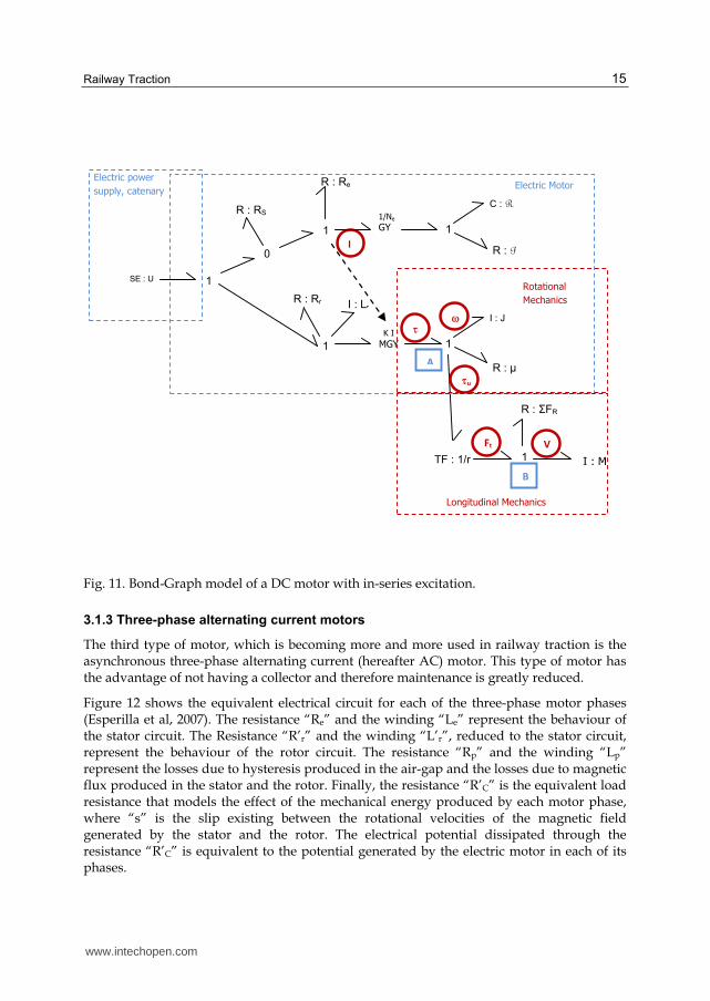
DC motors a with in-series excitation are very similar to those with independent excitation, except that the circuits of the stator and the rotor are connected in series. Therefore, the current flowing through both circuits is the same and is also what induces the magnetic flux that excites the rotor. As for the rest, everything stated concerning the independent excitation motor is applicable to the in-series excitation motor. Figure 10 depicts the outline of an electromechanical DC motor with in-series excitation, while Figure 11 shows its corresponding Bond Graph.

Fig. 10. Electromechanical diagram of a DC motor with in-series excitation.

www.intechopen.com

Railway Traction 15

Fig. 11. Bond-Graph model of a DC motor with in-series excitation.

3.1.3 Three-phase alternating current motors

The third type of motor, which is becoming more and more used in railway traction is the asynchronous three-phase alternating current (hereafter AC) motor. This type of motor has the advantage of not having a collector and therefore maintenance is greatly reduced.

Figure 12 shows the equivalent electrical circuit for each of the three-phase motor phases (Esperilla et al, 2007). The resistance “Re” and the winding “Le” represent the behaviour of the stator circuit. The Resistance “R’r” and the winding “L’r”, reduced to the stator circuit, represent the behaviour of the rotor circuit. The resistance “Rp” and the winding “Lp” represent the losses due to hysteresis produced in the air-gap and the losses due to magnetic flux produced in the stator and the rotor. Finally, the resistance “R’C” is the equivalent load resistance that models the effect of the mechanical energy produced by each motor phase, where “s” is the slip existing between the rotational velocities of the magnetic field generated by the stator and the rotor. The electrical potential dissipated through the resistance “R’C” is equivalent to the potential generated by the electric motor in each of its phases.

I

SE : U 1

0

R : RS

A

Ft V

u

B

Electric power

supply, catenary

I : MTF : 1/r 1

R : ΣFR

Electric Motor

Longitudinal Mechanics

Rotational

Mechanics

1

1/Ne

GY

R : Re

C : R

1

R : P

1

I : Lr

K I

MGY

R : Rr

I : J

1

R : μ

www.intechopen.com

Reliability and Safety in Railway 16

Fig. 12. Equivalent circuit of an asynchronous three-phase AC motor.

Fig. 13. Bond-Graph of the asynchronous three-phase motor.

Figure 13 illustrates the complete Bond-Graph model of the asynchronous three-phase AC

motor. Each of the horizontal branches of the Bond-Graph models each of the phases of

the motor, starting out from the equivalent circuit shown in Figure 4. The three phases are

subjected to an alternating current “U”, 120º out of phase using the Metatransformer ports

shown to the left. The mechanical power generated by each phase is modelled by the

“MGY” ports shown to the left. This rotational mechanical power is added to the “1”

junction shown on the extreme right of the Bond Graph, so that it can be applied to the

motor shaft modelled by the Inertial port “I” with parameter “J”. The friction losses are

also taken into account, and these are represented in the resistance port “R” with

parameter “μ”.

MGY

MGY

MGY

MTF

MTF

MTF 1 0

R : Re

1

R : R’cR : R’r

I : Le I : L’r I : L’c

1 0

R : Re

1

R : R’cR : R’r

I : Le I : L’r I : L’c

1 0

R : Re

1

R : R’cR : R’r

I : Le I : L’r I : L’c

SE : U 0

Electric energy

supply, catenary

Rotational

mechanics

I : J

1

R : μ

Electric Motor

www.intechopen.com

Railway Traction 17

4. Motor regulation and traction control techniques

If we speak about electric motor regulation and locomotive traction control, then we also have to speak about power electronics. Even for the three motors dealt with in the preceding section, the technology used in each case varies a great deal. For the reasons already stated in the previous section, at present, research conducted in this field is focused on three-phase traction technology with asynchronous motors and a cage rotor, converters with thyristors, and, of course, control technology based on IGBT transistors and microprocessors. However, let us begin by reviewing the regulation of the two DC motors studied to then go on to the regulation of asynchronous three-phase AC motors. So as to reach a proper understanding of the logic of the regulation techniques used in each case, we will continuously refer to the behaviour equations of the motors that were dealt with in the previous section.

As already stated towards the end of Section 2.2, the ideal traction curve is a constant power

hyperbole. It is said to be optimum for traction because if the motors had this operating

curve their power could be put to full use, with large torques at low speeds and small

torques at high speeds, as Figure 5 shows. But at very low speed, that is when starting, the

motor’s rotational speed is very low and the torque that it is able to produce tends towards

infinity. This causes the adhesion forces to exceed their limit in the wheel-rail contact. In

addition, as will be seen further on, the intensity of the current flowing in the motors takes

on very high values that will lead to the destruction of the electrical circuits. For these two

reasons, during the starting process the torque supplied by the motor needs to be limited so

as not to exceed the adhesion limits. At the same time the intensity of the current flowing in

the motors is limited so as not burn out the electrical circuits.

On the other hand, as we shall demonstrate further on, the characteristic operational curves

of the motors (motor torque curves “τ”, dependent on the rotational speed “ω”), do not fit

exactly with the constant power hyperbole, while at high speeds, the torque supplied by the

motor is less.

From the above two paragraphs two very important conclusions can be reached that affect

the operational regulation of the motors:

a. During starting at very low speed, we must regulate the intensity of the current and the motor torque so that the motor will supply the maximum possible torque without exceeding the current limits or the adhesion limits in the wheel-rail contact, until the conditions of the constant power hyperbole are reached in the shortest possible time. This operation is called “starting regulation” or “constant torque regulation”.

b. Once the constant torque hyperbole has been reached, we must check how to regulate the motor function so that its characteristic “τ-ω” curve fits the constant power hyperbole. This is called “constant power regulation”.

The following sections will deal mainly with regulating the motors during starting and then their regulation under constant power. The conclusion to be drawn from all this is that by applying these regulation procedures, the electric traction motors are made to operate in three stages: initially under constant torque during starting: then under constant power at moderate and high speeds, and finally, following the characteristic curve of the motor at very high speeds. (see Figure 14).

www.intechopen.com

Reliability and Safety in Railway 18

Fig. 14. Characteristic torque-speed curve “τ-ω”.

4.1 DC motor regulation during starting with independent excitation

The diagram and equations (13) and (14), of the behaviour of a DC motor with independent excitation were examined in Figure 8. By simply analysing the rotor circuit of the said figure, the following equation for the rotor’s operating voltage “Ur”, may be deduced:

戟追 = E + 迎追荊追 = 計荊勅降 + 迎追荊追 (18)

From which we can find the value of the current intensity in the rotor “Ir”:

荊追 =腸認貸懲彫賑摘眺認 (19)

And by entering into equation (13), we can find the equation for the motor torque “”,

dependent on the angular velocity “”:

= K荊勅荊追 = K荊勅 腸認貸懲彫賑摘眺認 (20)

By taking equation (18) the following expression can also be found for the angular velocity

“”:

降 = 腸認貸眺認彫認懲彫賑 (21)

By analysing equations (19), (20) and (21), it emerges that:

1. During starting, when “ 0”, the intensity of the current in the rotor “Ir” is very high,

since “Ir Ur/Rr”, as the ohmic resistance of the rotor circuit “Rr” is very low. A very high current intensity may burn out the circuits. For this reason, current intensity must be limited during starting.

2. The motor torque “” during starting is also very high and gradually drops as the

motor’s angular velocity “” increases. In principal, this is sufficient as the behaviour is similar to that of a constant power hyperbole (remember Figure 5). But during starting, the torque supplied by the motor is so high that it exceeds the wheel-rail adhesion limit. To avoid slip, the starting torque needs to be limited to the allowable values of the adhesion.

τ [N·m]

ω [rad/s]

Constant power hyperbole

Constant torque

Characteristic curve of motor at maximum speed

www.intechopen.com

Railway Traction 19

3. Consequently, during starting the current intensity must be limited to avoid the circuits burning out and to limit the motor torque, thus preventing the adhesion in the wheel-rail contact from exceeding the limits. The maximum motor torque obtained during starting is called “maximum continuous torque”, (see Figure 16). Since the motor torque and the tractive effort “Ft” in the wheel-rail contact are directly related, the maximum available tractive effort “Ft” during starting is also called “maximum continuous effort”, (see Figure 5).

Fig. 15. Shunting of DC motors with independent excitation.

When dealing with DC motors with independent excitation the most effective way of reducing motor torque during starting is to reduce the intensity of the current in the stator “Ie”, as in equation (20). To this end, a rheostat is placed in series with the stator, with a variable resistance “Re”, as can be seen in Figure 15. This is known as “Shunting”. As the intensity “Ie” diminishes, the motor speed increases (equation (21), without any excessive

increase in the motor torque “”. At the beginning of starting, the value of the Shunting resistance “Re” is maximum, producing a maximum reduction of the current intensity “Ie” and therefore, the magnetic flux induced in the rotor is minimum. This operation is

controlled so that the motor torque “” will be the maximum appropriate one without exceeding the adhesion limits. As the locomotive gradually gathers greater speed, the

intensity “Ir” and the motor torque “” gradually decrease (equations (19) and (20). It is then necessary to increase the motor torque to recover traction capability during starting. To achieve this, the value of the Shunting resistance “Re” is gradually reduced in a controlled

manner. Thus, the current intensity “Ie” and the motor torque “” again increase without exceeding the adhesion limits and recover the locomotive’s traction capability (see the “real operational curve” in Figure 16).

Below, we have simulated the operation of a DC motor with independent excitation using the model shown in Figure 9, for different fixed values of the Shunting resistance “Re”. The motor has a power of 1200 kW and in the simulation was working under zero load. Figure 16 shows the results of the motor torque obtained for different fixed values of “Re” as a function of the motor’s rotational speed, comparing the results with the theoretical torque corresponding to the constant torque hyperbole and also to the maximum continuous torque.

www.intechopen.com

Reliability and Safety in Railway 20

Fig. 16. Simulation results of a DC motor with independent excitation for different values of the Shunting resistance “Re”.

4.2 Regulation during starting of DC motors with in-series excitation

The behaviour of a DC motor with in-series excitation is similar to that of a DC motor with independent excitation, but there is one very important difference: the current flowing in the rotor and the stator is the same (see Figure 10). Following a similar procedure to that in the preceding section, we will now find the behaviour equations for the DC motor with in-series excitation. The following equation considers a total fall in the voltage in the motor according to the intensity of the current:

U = E + 迎追荊 = 計荊降 + 迎追荊 (22)

From which we can find the value of the current intensity flowing through the motor “I”, according to the operational voltage and the already known parameters of the motor, “K” and “Rr”:

荊 = 腸懲摘袋眺認 (23)

By entering into equation (13), the equation for the motor torque “” can be found according

to the angular velocity, “”, since the current intensity flowing through the rotor and the stator is the same:

= K荊勅荊追 = K荊態 = K 岾 腸懲摘袋眺認峇態 (24)

By analysing equations (23) and (24), similar conclusions can be drawn as from the case of the DC motor with independent excitation:

1. During starting when “ 0”, the current intensity “I” is very high since “I U/Rr”, as the ohmic resistance of the rotor circuit “Rr” is very small.

2. The motor torque “” during starting is also very high and gradually decreases as the

angular velocity of the motor “” increases. 3. Consequently, during starting, the current intensity needs to be limited to avoid the

circuits burning out and to limit the motor torque, thereby preventing the adhesion limits being exceeded in the wheel-rail contact.

www.intechopen.com

Railway Traction 21

In the example of the DC motor with in-series excitation, the above is achieved by inserting resistances in series with the motor, as can be seen in Figure 17. At the beginning of starting the maximum number of starting resistances “Ri = R1 + R2 + R3” are connected to produce the maximum reduction of current intensity “I” and therefore, the maximum reduction of

the motor torque “”. As the locomotive gathers greater speed, the intensity “I” and the

motor torque “” gradually decrease. Then it is necessary to increase the motor torque to recover traction capability during starting. By means of the connections A, B and C, the resistances are successively bridged, and, therefore, cease to function and the starting resistance “Ri” gradually decreases in value. So, in a controlled manner, the current intensity

“I” and the motor torque “” again increase and the locomotive recovers its traction capability (see “real operational curve” in Figure 18).

The operation of a DC motor with in-series excitation has been simulated using the Bond-Graph model shown in Figure 11, with variable starting resistances. For this simulation, since the starting resistances are placed in series with the motor, they are taken into account by adding them to the rotor resistance “Rr, through the Resistance port “R:Rr”, (see Figure 11). The motor under consideration has a power of 1200 kW and in the simulation was working under zero load. Figure 18 shows the results obtained for the motor torque according to the rotational speed of the motor for different values of the starting resistances “Ri” and comparing the results to the theoretical torque corresponding to the constant power hyperbole, as well as to the maximum continuous torque.

Fig. 17. Resistances in series with the motor in starting mode.

www.intechopen.com

Reliability and Safety in Railway 22

Fig. 18. Simulation results of a DC motor with in-series excitation for different values of the starting resistances “Ri”.

Fig. 19. Starting diagram of a locomotive with two traction motors.

Locomotives usually have several motors and starting can also be controlled by combining the incorporation of resistances in series, “Ri“, of each motor with the motors being connected in series. Figure 19 shows a schematic outline of the electrical connection of a locomotive that has two traction motors. Both have resistances in series for the starting, and in addition, switches A and B are installed so as to be able to connect both motors in series or in parallel. When the motors are connected in series, the voltage in them is half the nominal voltage, and, as a result the intensity flowing through them is also half, reducing

the starting torque “” to half. In this way, the resistances “Ri” during the starting of each motor can be less, resulting in fewer energy losses during starting. Initially, when the train is gathering speed, the starting resistances “Ri” are gradually reduced. At a given instant, the in-series connection of the motors is switched to in-parallel and the starting resistances “Ri” are slightly increased. Finally, when the train reaches a determined speed the process is concluded by cancelling the starting resistances “Ri”.

TRACK

SWITCH A SWITCH B

CATENARY

U

MOTOR 1

MOTOR 2

www.intechopen.com

Railway Traction 23

4.3 Regulating the behaviour of DC motors with in-series excitation, with the constant power hyperbole

When the starting period of the motors has been exceeded (section A-B in Figures 16 and 18), we must deal with controlling the motor in order to fit its behaviour to the constant power hyperbole.

The Electromotive Force “E” induced in the rotor by the stator is proportional to the magnetic flow “Φ” and the angular velocity of the rotor’s rotation “ω”, (Karnopp, 2005):

継 = 計沈 Φ降 (25)

Where “Ki” is a constant associated with the stator winding.

From the above equation we can calculate the angular velocity “ω”:

降 = 帳懲日地 (26)

Also, from equation (22), we can obtain the following expression for the value of the Electromotive Force “E”:

E = U 伐 迎追荊 (27)

By substituting equation (27) in equation (26), we obtain:

降 = 濁貸眺認彫懲日地 (28)

From this it may be deduced that a given voltage can increase the motor’s rotational speed by reducing the flux “Φ” of the stator. As we also know, this flux depends on the current flowing through the stator, because as we are dealing with in-series excitation, it is the same as that flowing through the rotor. To change the current in the stator (and, therefore, the induced flux), without changing that of the rotor, an assembly is used like the one in Figure 20, where a rheostat is installed in parallel to the stator. As the resistance of the rheostat gradually decreases, the part of the current flowing through the stator becomes less and as a result, the flux “Φ” decreases.

The control of direct current motors, based on reducing the current passing through the stator, is called “Shunting” the motors. This term was used in section 4.1., (Figure 15), when dealing with the starting of DC motors with independent excitation.

Fig. 20. Shunting DC motors with in-series excitation.

www.intechopen.com

Reliability and Safety in Railway 24

The shunting “α” of a motor is defined as:

糠 = 彫貸沈彫 ∙ などど (29)

By shunting the motor, its characteristic curves move towards the right, the bigger the move, the greater the shunting percentage. This can be seen in Figure 21, where the shunting curves are shown, continuing the behaviour simulation of the DC motor with in-series excitation carried out in Section 4.2, once the starting period had been completed (section A-B”).

It is not possible to totally decrease the current in the stator as it depends on how the motor is constructed. It can usually only be shunted up to 55%, because with higher values switching problems arise in the motor.

Fig. 21. Torque curves on shunting the DC motor with in-series excitation.

4.4 Electronic regulation of direct current motors

During the simulations carried out on the behaviour of the motors, the previous sections

have taken account of the discrete values for the starting resistances or for the shunting

resistances. This has enabled us to display the corresponding torque curves. However, the

real operating curve, as Figures 16, 18 and 21 may recall, jumps up and down as it attempts

to firstly fit to the continuous torque straight line and then to the constant torque hyperbole.

This was how the operation of a real motor was originally regulated. It can currently be

highly valid during a computer simulation for understanding the phenomena that occur.

However, with the development of power electronics, these proceedings for regulating the

operation of motors are not the most appropriate.

The electronic regulation of direct current motors is essentially based on regulating the feed

voltage. The devices used to do this are called Choppers.

When dealing with a motor with independent excitation a complete regulation can be

achieved by controlling the stator and rotor voltage separately. If the motor has in-series

excitation, the feed voltage to the rotor and the stator Shunting must be controlled

simultaneously.

www.intechopen.com

Railway Traction 25

The chopper’s mission is to act as a switch to open and close the motor feed circuit, as Figure 22 illustrates. In this way, by starting with a fixed continuous feed voltage “U” in the catenary, a variable voltage applied to the motor is obtained which manages to regulate its speed. Since the switch is off (driving the chopper) the catenary voltage is applied to the motor to make an electric current flow through the motor. When the switch is opened the voltage applied to the motor is cancelled, cutting off the current to the switch. During the time the switch is on, the motor current flows through the diode placed in parallel. By varying the times the switch is on and off, the mean voltage in the motor can be varied and therefore, the current intensity flowing through it. This method perfectly manages to regulate the motor torque and perfectly follows the theoretical continuous torque curve (starting), and the constant power hyperbole without any steps appearing in the real torque operating curve mentioned at the beginning of this section. To achieve this phenomenon, devices called Thyristors are used.

Fig. 22. Principle of how a Chopper-controlled DC motor functions.

4.5 Alternating current motors

In the last 30 years railway traction motors have ceased to be direct current motors controlled by the connection and disconnection of resistances to become asynchronous alternating current motors controlled by IGBT transistors for medium powers, or GTO thyristors through the use of pulse width techniques for high powers (Faure, 2004).

As explained in the previous sections, the first controls using rheostats for direct current motors gave way to thyristor-based control. DC motors can be better controlled by this technology by avoiding the transitory “jerk”, effects caused by connecting and disconnecting the starting and shunting resistances. So, thyristors led to a much better and uniform functioning of DC motors. Notwithstanding, the drawbacks derived from the collector still existed, which required large-size motors that needed frequent maintenance. These requirements became much less with the appearance of synchronous alternating current motors and were practically eliminated with the asynchronous motors.

The development of traction control systems has led to the use of simpler, more robust and cheaper asynchronous motors. They are more complicated to regulate than synchronous motors but this complexity became much less with the development of IGBT transistors. Nowadays, the major research and development projects are focussing on the technologies related to asynchronous alternating current motors (hereafter asynchronous AC motors).

U

CHOPPER

MOTORDIODE

I

www.intechopen.com

Reliability and Safety in Railway 26

The three-phase asynchronous motor is an induction motor based on the generation of rotating magnetic fields by means of the stator windings, which induce electric currents in the rotor windings. Due to the interaction between these induced currents and the magnetic fields, forces are generated in the conductors that produce a motor torque. If the rotor rotates at the same speed as the magnetic fields, there is no variation of flux passing through the turns of the rotor and the induced current is zero. For a motor torque to be produced there needs to be a difference (slip) between the angular velocities of the magnetic field and the rotor.

For a low frequency alternating electric current, the torque generated by the motor “τ” satisfies an expression that is similar to the expression for direct current motors:

= K辿Φ荊追 = K荊勅荊追 (30)

Where, “Ki” and “K” are behaviour constants of the motor; “Φ” is the magnetic flux generated by the stator, and “Ir” is the intensity of the current flowing through the rotor. It may be deduced from this expression that in DC motors, the torque increases along with the intensity of the current in the rotor.

However, it is also known that the current in the rotor is proportional to the magnetic flux “Φ” generated by the stator and to the slip “s” between the rotor and the magnetic field. Moreover, the magnetic flux “Φ” is proportional to the quotient between the feed voltage “U” and the current frequency “f”, which means the torque can also be expressed as:

= K脱 岾濁脱峇態 s (31)

Where “Kf” is a new constant of the motor function. The law expressed by equation (31) is valid for small slips, but for larger slips the ratio ceases to be linear. Figure 23 shows the motor torque curves “τ” compared to the rotational velocity “ω”, for different values of the current frequency “f”.

Fig. 23. Torque curves for an AC asynchronous squirrel cage motor.

0

5

10

15

20

25

30

35

0,00 10,00 20,00 30,00 40,00 50,00 60,00 70,00 80,00 90,00 100,00

Maximum continuous torque, (kN.m).

Constant power hyperbole, (kN.m).

τ (kN.m) (f=1 Hz) (U=7 kV)

τ (kN.m) (f=5 Hz) (U=16 kV)

τ (kN.m) (f=10 Hz) (U=22 kV)

τ (kN.m) (f=15 Hz) (U=25 kV)

(rad/s)

(kN.m)

www.intechopen.com

Railway Traction 27

By regulating AC motors and fitting their working to the theoretical torque-speed curves “τ-ω”, that is to say, starting under constant torque and constant power hyperbole (remember Figure 14), the feed voltage “U” and the current frequency “f” can be varied simultaneously. To achieve this, IGBT, GTO thyristor-based technologies are used for high powers, which modulate the width of the electric pulses through the superposition of a triangular wave and a voltage signal that is proportionate to the signal required. Doing this will ensure that the motor describes the constant torque curve and constant power hyperbole without any steps.

Figure 23 shows the torque-speed curves for an asynchronous squirrel cage AC motor with a power of 1200 kW, simulated using the Bond-Graph model dealt with in Figure 13, for different frequency values of “f” and the operating voltage “U”. Obviously, by a continuous regulation of the frequency and voltage, the real working of the motor will exactly fit the constant torque straight line during starting and the constant power hyperbole.

5. Prospects, current and future lines of research, conclusions

Obviously, for lack of space, a whole range of issues have been left undealt with, but they are of no less importance: maximum starting efforts and couplings, load capacity and in-service power, the influence of the vehicles’ lateral and vertical dynamics, generation systems, energy transport and capture, pantographs and floaters, service automation and traction control, regenerative brakes and energy recovery systems, and a long etcetera.

As a final conclusion, the most current areas of progress in research, development and innovation and their future prospects are mainly directed towards achieving a railway that is better adapted to the new global needs of mobility, sustainability and respect for the environment:

a. More efficient systems for generating, transporting, capturing, transforming, utilising, regulating and recovering energy.

b. Traction control and service automation systems, regenerative braking and energy storage systems, reversible electrical supply sub-stations and rail traffic management.

c. Multidisciplinary optimisation of infrastructure and vehicle design. d. The design implications of vehicles, infrastructures and systems in energy consumption

and the environmental impact of transport. e. Optimisation of vehicles and infrastructures for their use in multimodal systems. f. Calculation systems, predicting and optimising energy consumption and emissions. g. Foreseeable consequences of technological development on the innovation of vehicles

and infrastructures for sustainable mobility.

6. References

Andrews, H.I. (1986). RailwayTraction. The Principles of Mechanical and Electrical Railway Traction. Ed: Elsevier. ISBN: 0-444-42489-X.

Coenraad, E. (2001). Modern Railway Track. Ed. Delft University of Technology. ISBN: 90-800324-3-3. Delft, Holanda.

Esperilla, J.J., Romero, G., Félez, J., Carretero, A. (2007). “Bond Graph simulation of a hybrid vehicle”. Actas del International Congress of Bond Graph Modeling, ICBGM’07.

www.intechopen.com

Reliability and Safety in Railway 28

Faure, R. (2004). La tracción eléctrica en la alta velocidad ferroviaria (A.V.F.), Colegio de Ingenieros de Caminos, Canales y Puertos, ISBN 84-380- 0274-9, Madrid, España.

Iwnicki, S. (2006). Handbook of Railway Dynamics. Ed. Taylor & Francis Group. ISBN 978-0-8493-3321-7. London, Reino Unido.

Karnopp, D.; Margolis, D.; Rosenberg, R. (2000). System Dynamics: Modeling and Simulation of Mechatronic systems. Ed. John Wiley & Sons, LTD (2ª). Chapter 11. ISBN: 978-0-471-33301-2. Estados Unidos.

Karnopp, D. (2005). Understanding Induction Motor State Equations Using Bond Graphs. Actas del International Congress of Bond Graph Modeling, ICBGM’05.

Lozano, J.A.; Félez, J.; Mera, J.M.; Sanz, J.D. (2010). Using Bond-Graph technique for modelling and simulating railway drive systems. IEEE Computer Society Digital Library (CSDL), 2010 12th Congress on Computer Modelling and Simulation. ISBN 978-90-7695-4016-0. BMS Number CFP1089D-CDR. Cambridge, Reino Unido.

www.intechopen.com

Reliability and Safety in RailwayEdited by Dr. Xavier Perpinya

ISBN 978-953-51-0451-3Hard cover, 418 pagesPublisher InTechPublished online 30, March, 2012Published in print edition March, 2012

InTech EuropeUniversity Campus STeP Ri Slavka Krautzeka 83/A 51000 Rijeka, Croatia Phone: +385 (51) 770 447 Fax: +385 (51) 686 166www.intechopen.com

InTech ChinaUnit 405, Office Block, Hotel Equatorial Shanghai No.65, Yan An Road (West), Shanghai, 200040, China

Phone: +86-21-62489820 Fax: +86-21-62489821

In railway applications, performance studies are fundamental to increase the lifetime of railway systems. Oneof their main goals is verifying whether their working conditions are reliable and safety. This task not only takesinto account the analysis of the whole traction chain, but also requires ensuring that the railway infrastructureis properly working. Therefore, several tests for detecting any dysfunctions on their proper operation havebeen developed. This book covers this topic, introducing the reader to railway traction fundamentals, providingsome ideas on safety and reliability issues, and experimental approaches to detect any of these dysfunctions.The objective of the book is to serve as a valuable reference for students, educators, scientists, facultymembers, researchers, and engineers.

How to referenceIn order to correctly reference this scholarly work, feel free to copy and paste the following:

José A. Lozano, Jesús Félez, Juan de Dios Sanz and José M. Mera (2012). Railway Traction, Reliability andSafety in Railway, Dr. Xavier Perpinya (Ed.), ISBN: 978-953-51-0451-3, InTech, Available from:http://www.intechopen.com/books/reliability-and-safety-in-railway/railway-traction

© 2012 The Author(s). Licensee IntechOpen. This is an open access articledistributed under the terms of the Creative Commons Attribution 3.0License, which permits unrestricted use, distribution, and reproduction inany medium, provided the original work is properly cited.