raising irrigation productivity and releasing water …

Raising Irrigation Productivity and Releasing Water for Intersectoral Needs - RIPARWIN,

RAISING IRRIGATION PRODUCTIVITY AND RELEASING WATER FOR INTERSECTORAL NEEDS

(RIPARWIN)

Final Report - Irrigation Productivity Paradigms - IPP

INFORMED FROM

THE PLAINS

Irrigation efficiency and productivity can be measured at the scale of a whole irrigation system, at the individual

plant scale, and at almost any level in between

Irrigation Productivity Paradigms - IPP

By: Machibya Magayane August 14, 2002


Table of Contents Page List of Figures...............................................................................................................3 List of Tables ................................................................................................................3 List of Acronyms..........................................................................................................3 Glossary of Symbols.....................................................................................................4 Definition Table............................................................................................................4 Preamble .......................................................................................................................5 Defining Irrigation Efficiency.....................................................................................6 Summary.......................................................................................................................8 1. Introduction........................................................................................................8 2. The case study ....................................................................................................9 3. Description of the study sites ..........................................................................10

3.1 The Kapunga large irrigation scheme (NAFCO system)........................................................10 3.2 The Kapunga smallholder irrigation scheme (improved system) ...........................................10

3.3 The Mwashikamile top and end farm (Traditional systems) ..............................................10 4. Methods and data collection ...........................................................................11 5. Results and discussion .....................................................................................11

5.1 Defining wet and dry year ......................................................................................................11 5.2 Classifying the years of the study period................................................................................11

6. Water use in irrigated rice ..............................................................................12 6.1 NAFCO and Smallholder calculations of efficiency - Net and gross water demand method. 12

6.1.1 Calculation of efficiencies ..............................................................................................13 6.2 NAFCO and smallholder calculation of efficiency - water depths maintained in fields method 14

6.2.1 Modelling water depths in fields and net depth ..............................................................14 6.2.2 Summary and calculation of efficiency based on depths ................................................15 6.2.3 Canal/furrow conveyance efficiency - Upstream and downstream discharge method ...15

7 Water productivity in irrigated rice ..................................................................17 7.1 Introduction ............................................................................................................................17 7.2 Summary ................................................................................................................................18

7.2.1 Local productivity...........................................................................................................18 7.2.2 Basin productivity...........................................................................................................18

7.3 Irrigation efficiency - productivity method ............................................................................18 7.3.1 Calculated efficiencies - productivity method ................................................................18

7.4 Hard thinking on efficiency values added by drain water in river basin ......................................20 7.3.1 Temporal Efficiency (TE)......................................................................................................20 7.3.2 Early harvested rice fetches good price - an efficiency indicator ...................................22

7.5 True system efficiency in water reuse practices .....................................................................24 7.6 Generalized efficiency pattern for the KWS...........................................................................27

8 Conclusions and Recommendations ..................................................................29 9 References ............................................................................................................30 APPENDIX 1: River network of the KWS and maximum cropped area for 1999/2000 (3829 ha)....................................................................................................32 APPENDIX 2: The KWS appearance before emergence of the drain water users and canal networks. ...................................................................................................32 APPENDIX 2: The KWS appearance before emergence of the drain water users and canal networks. ...................................................................................................33 APPENDIX 3: Gross margin for rice production in Usangu ...............................34



List of Figures Figure 5.1. Monthly rainfall recorded during the study period....................................11 Figure 5.2. Annualised rainfall amount for the study period.......................................12 Figure 6.1: Water movement in bunded rice fields......................................................14 Figure 7.1. Water velocity in different canals..............................................................21 Figure 7.2. Rice price fluctuation in the KWS for 1999/2000 season .........................23 Figure 7.3. Rice price fluctuation in the KWS for 2000/2001 season .........................23 Figure 7.4. Generalised efficiency pattern for Usangu irrigation systems .................27 List of Tables Table 6.1: summary of water use 1999/2000 season (dry year) ..................................13 Table 6.2: summary of water use 2000/2001 season (wet year)..................................13 Table 6.3. Mean water depths (mm) kept in fields for 1999/2000 and 2000/2001 seasons .........................................................................................................................15 Table 6.4 Efficiencies of irrigation systems- water depth method ..............................15 Table 6.5: The conveyance efficiency of different canals ...........................................16 Table 6.6: Water velocity in the canals of the KWS - colour tracer method...............17 Table 7.1. Summary of water productivity 1999/2000................................................19 Table7.2. Summary of water productivity 2000/2001.................................................19 Table 7.3. Factors causing delay of water to the downstream farm in the KWS.........22 List of Acronyms AfDB The African Development Bank BE Biological Efficiency CP Crop performance Dp Deep Percolation Water Effic. Efficiency Eqn. Equation GIS Geographical Information System GPS Global Positioning System KWS Kapunga Water System LP Lateral percolation MC Moisture Content/ Main Canal MSV Mean System Velocity N/A Not Applicable NAFCO National Agricultural and Food Co operation S.holder Small holder or smallholder scheme/farm SMUWC Sustainable Management of the Usangu Wetlands and its Catchment SP System productivity SWMRG Soil and Water Management Research Group TE Temporal efficiency IWMI International Water Management Institute TW Transect Walk UWE Water Utilisation Efficiency SE System Efficiency PCT Paint Colour Tracer Sec. Second SC Secondary Canal D Drain canal WMO World Meteorological Organisation Tshs. Tanzanian Shillings ( 1USD = 950 Tshs in March 2002)



Glossary of Symbols *S Subsurface Movement of water within the field Ad Area in the downstream farms At Total area of an irrigation system Au Area in the upstream farms cm Centimetres CPd Crop performance in the downstream farms CPu Crop performance in the upstream farms cumec Cubic meters per second ec Water Conveyance Efficiency ed Downstream efficiency Es System efficiency Et True efficiency eu Upstream efficiency Ev Evaporation Water I Irrigation Water k Ratio of eu to edL Length l Litres m Metres mm Millimetres Pd Price existing in the markets when harvesting commence at the downstream Pu Price existing in the markets when harvesting commence at the upstream R Raingauge/Rainfall r Ratio of (Pd) to (Pu) Ro Runoff water Tr Transpiration water t Tonnes Kg Kilograms $ US Dollar

Definition Table Downstream The area where water leaving a field, farm or scheme does go Gross margin Net return which is obtained after selling rice Gross revenue Income obtained from rice before cost of expenditure is subtracted Mbuga Low land (downstream) areas with fertile alluvial soils where rice

production is done. Peri-NAFCO fields Fields surrounding NAFCO/large irrigation schemes Plot Big bunded rice fields (common in large irrigation schemes). The size is

between 5 and 10 ha. Subamati, Zambia, Kilombero and India rangi

Rice varieties available in the Kapunga Water System

System The area using common source of water Upstream The area where water coming to the field, farm or scheme originate Variable costs Cost incurred during rice production Vijaruba/Jaruba Small bunded rice fields (common with indigenous farmers). The size

may range from 20m2 to 400m2



Preamble Irrigation accounts for over 70% water with draw world-wide and even more in developing countries (Kay,1999; Bryan 2000). While over many years it was believed that the science of water diversion and careful in field distribution is what was important to bring about effective water use, the current debate informs that the water management is what is more important and it could bring about effective water use (Kay 1999). While the sophisticated science behind improved headwork, canals, and overall conveyance system has over many years failed to raise irrigation efficiency in surface irrigation and therefore remaining below 50%, it has recently been reported that irrigation efficiency could be raised to 100% in river basins (Seckler, 1985; Keller, 1996). The main proposition is that certain paddy irrigation systems, unlike those for other crops, are basically self-regulating in allocating water between farmers and therefore do not require active management to ration water at field level. And it has therefore being argued that resources that are being allocated to promote improvement at field level are being wasted and it should be deployed elsewhere. Therefore a debate about river basin management approach is brought about these two different thoughts. Those who believe that irrigation efficiency in river basin is currently high enough and self regulating, they argue that a river basin management is not necessary while the conventional thought is concern with improving intakes, lining canals and proper water management. While many authors have presented and some even challenged these two thoughts in isolation, very few have drawn the subjects coherently to express the similarities and the differences. And as measuring irrigation efficiency in either of the two approaches might be notoriously difficult, many of the reported figures in papers and books effectively do not show methods in which they were obtained and/or measured. As due to this, the debate between the two thoughts is growing with no clear way of reaching a concession. This has lead to many of them to outweigh most important factors that could otherwise either improved their thoughts or arrive at realistic ways of measuring efficiency and managing water resources. Indeed this scale of difference in understanding has created a gap and therefore delaying to bring together the knowledge of river basin management, which exists between the two schools of thought. This document attempts to address this gap in understanding and approaches to irrigation efficiency analysis. It presents a broader view of analysis through a two years study undertaken in the Usangu basin Tanzania on which both thoughts were tested. The results are presented through three different subtopics being arranged in a chronological order to give you the insight of the two thoughts. The first subtopic present the irrigation efficiency as always defined by conventional methods while the second subtopic as defined by both schools. The last subtopic discusses in details the successes and shortfalls of both thoughts. It is hoped that this document will provide fresh insights for both sides and that it will inspire them to take up these challenges. Machibya Magayane August 6, 2002



Defining Irrigation Efficiency We must first deal with the problem of defining efficiency of irrigation. The first problem encountered is the level or scale at which it is measured. Efficiency can be measured at the scale of a whole irrigation system, at the individual plant scale, and at almost any level in between. The scale of measurement depends on the focus of the person doing the measuring. The scale of measurement is of critical importance in tackling the issue of improving efficiency, and must be matched to the target audience. For example, when measuring on-farm efficiency, too broad a scale makes it difficult to determine what the causes of low efficiency are and what can be done to improve the situation. Going to a smaller scale excludes the consideration of wider issues, such as delivery system losses and inefficiencies, but is necessary to clearly identify real opportunities for improvement at the individual property/manager scale. This raises a second problem with defining efficiency of irrigation, any definition will depend to a large degree on the outlook of the person producing the definition. Those managing the supply of water tend to see efficiency simply in terms of losses in the delivery system, or the gross amount of water consumed by each of their customers as compared to some average or ideal figure. Irrigators are more interested in how much product, or perhaps how much profit, they can produce with a given amount of water. Finally, those involved in resource management are more interested in reducing wastage of the resource, especially where such wastage has negative off-site impacts on the environment. As all of these factors are important in the larger picture, no one definition of efficiency is complete. If a realistic attempt is to be made to quantify and compare efficiency of irrigation, a range of measures or indicators is required, in order to capture all of the important factors involved (Skewes et al., 1998) Irrigation Efficiency (%): Irrigation efficiency (equivalent to application efficiency as defined by the On-Farm Irrigation Committee of the Irrigation and Drainage Division, 1978) assesses the relative percentage of irrigation water applied to the crop that was directly used by the plants for evapotranspiration. High values for irrigation efficiency reflect low volumes of drainage produced throughout the irrigation season. For the realistic attempt in analysing irrigation efficiency, the next outlined indicators would be important. Yield (t/ha): Yield per hectare is the traditional way of representing the performance

of an agricultural enterprise. While it is of immediate interest to irrigators, it can sometimes give a false impression of efficiency, when other inputs are not being used efficiently.

Water Use Efficiency (t/m3): Water use efficiency is defined as tonnes of produce per meter cubic of irrigation used in the production cycle. Even if yield per hectare is high, using excessive amounts of irrigation water to achieve that high yield is not an efficient use of a limited resource. Seckler 1985 in the laissez-faire concept produced a fine plant yield water relationship whereby, findings indicates that when excess water are supplied to a paddy plant, a limit is reached when yield (Kg) starts to decrease. In most areas, there is sufficient land available (including Usangu basin) in reasonable proximity to the river, but there is no new water



available to apply to that land. It could be argued, on this basis, that water use efficiency, or yield per meter cubic of irrigation, is far more important than yield per hectare in making the most efficient use of the limited resources available for irrigation.

However if the produces are fruits (t/m3) indicator will have to measure the relative

quality of the product of irrigation. The use of this indicator is obviously limited to crops which are packed for fresh fruit markets. Producing large tonnage of poor quality fruit is not necessarily a good use of a limited resource. Good and packable fruit is the clear focus of many farmers and business man, and therefore the production of packed fruit per unit of water is a much better indicator of productive use of water than gross tonnes produced per unit of water in this case.

Alternatively a sellable produce will be a good indicator ($/m3): Return per meter

cubic assesses not only the amount of produce, but also the quality of the produce, measured by its value. Skewes et al 1998 used a standardised structure of returns applied to the tonnages of produce in each of a range of quality classes (specific to each crop), to compare the overall return on irrigation water.

Cost of Water per Tonne of yield ($/t): Cost of water per tonne of yield measures the monetary value of irrigation water used to grow a tonne of yield at each site. It reflects not only how much water was used per tonne of yield, but also the cost structure of the site, and the likely sensitivity of the site to increases in the cost of water.

Return per Dollar Water Input ($/$): Return per dollar water input takes return per meter cubic another step, by making a direct comparison of dollars spent on water with dollars returned from the use of that water. Obviously a low return per dollar water input is of concern, as it impacts directly on the profitability of the enterprise

Yield per Volume of Drainage (t/m3): Yield per volume of drainage is similar to water use efficiency, except that it relates the yield produced to the volume of drainage produced, rather than to the volume of irrigation applied. The logic behind this indicator is related to the understanding that some drainage is required for leaching of salt from the rootzone, but excessive drainage is counter-productive. If drainage is necessary, we can measure the positive utility of that drainage by comparing it to the level of production associated with its generation. High yields per drainage volume indicate a high ratio of return (production) to cost (drainage). Low yield per drainage volume indicates a poor return to cost ratio, and suggests that the levels of drainage produced are excessive. However Keller, 1996 in his conceptual model of water reuse has defined the importance of drainage in river basin as to increase efficiency in which the irrigation water eventually generate up to 100% efficiency.



Summary Generalising figures of water uses, productivity or irrigation efficiency for surface irrigation systems it has been a normal quote by many water specialists, which in many cases leads to erroneous conclusion with regards to water allocation and management. While most of large and improved water righted schemes in Tanzania are managed conventionally (i.e. at prior known water requirement per area), most of traditional irrigation systems do not operate in a similar fashion. The available water and ability of farmers to trickle water from one field to another to as far as possible define the area of most traditional systems. This document summarises a comparative study on paddy water use and productivity of three farms arranged serially from the headwork (Top, Middle and End) in a way allowing water reuse between the three farms/schemes. The top scheme was modern followed by an improved scheme while the traditional scheme was positioned at the tail end. While the competition of water was observed to be relatively higher as you go downstream, the decrease in annual volumetric water use in fields as you go downstream was also apparent. Key words: Irrigation, Efficiency, and Water-use

1. Introduction Most surface irrigation systems are widely reported to operate at lower efficiency values (Figures of 30% - 40% are frequently quoted). While surface irrigation accounts for about 95% of world irrigation, the worldwide contribution of irrigation to food production is over 40% from just 17% of the land cultivated (Kay, 1999). This therefore suggests that about 38% of world food production come out of surface irrigation. While the world is set to be 20% short of fresh water by 2025 conversely, the world population is set to grow by 50% during the same period. As the future need of food requirement especially in Africa is compared to increase in population, expansion of irrigated agriculture cannot be escapable (Gowing et al, 1994). This volume is concern with situation in the Usangu basin part of the Rufiji basin in Tanzania. In Usangu, there exists three types of irrigation systems namely NAFCO, Improved smallholder and traditional systems (Gillinghum, 1999). The total area irrigated in the basin is estimated at 43,000 ha (SMUWC, 2001). Of the total irrigated area, smallholders cover an area of about 75% in the basin. Though generalisation is common for all surface irrigation systems, indeed the field design, distribution canals, cropping pattern and calendar and water management differs between these systems. These factors bring about necessary different water use efficiency and productivity between the three systems.



While researchers have put up many of the ideal water requirement for rice production, very few have been utilised for efficiency analysis in different irrigation systems. Sir Halcraw et al, 1992; Wim et al, 2001 have for example recommended an amount of 900 - 1500 mm for rice requirement through various techniques which averages at 1100 mm in tropics and sub tropics. Other researchers on water losses from rice fields have worked for required depths in fields. Walker, 1987 estimated the ideal water depth required in rice field through various methods and found out to be 50 mm for minimum losses in fields. Further rice productivity at proper management is informed to range between 0.7 - 1.1 kg/m3 at 15 - 20% moisture content (Doorenbos, 1986). While the global water duty of 2 litres per second per hectares is applicable nearly world wide, rarely the efficiencies is analysed based on these research findings. This document is testing several paradigms on efficiency and productivity via a transdisciplinary approach as described next.

2. The case study For many years now, great emphasis has been placed on effective water use in many irrigation systems. The work reported here focuses on the Kapunga water system, in which volumetric water uses and productivity of three different types of irrigation systems was determined. Appropriate experimental site from each farm was selected. The aim of site selection was to have a site that would allow thrice to fourth times drain water recycling/reuse - the practice common with most Usangu irrigation systems. This was important in a sense this research apart from doing exploratory work, it was designed to test different ideas and concepts that are relevant to river basin management. The water reuse is widely reported now days in the field of irrigation efficiency particularly in river basins and it is thought that through this practice, efficiencies of irrigation systems are raised (Seckler, 1985). Such a design and practice was observed in many irrigation system in Usangu but that of the Kapunga farms had some other more added advantages for this investigation as explained here next. Recycling of water between selected sites could be arranged in such a way that water which is diverted for the first site in the (NAFCO farm) is reused immediately at the second site (Smallholder farm) and so onto the third farm (traditional farm) before water returns to the source river - therefore minimal losses could be attained. Further the Kapunga farms would allow easy and careful siting of the experimental sites with reference to condition of water availability. The experimental sites had to have definable areas - of which the Kapunga water system was perfect, though the rice areas would change dramatically within irrigation systems as water supply changes. The selected sites had in addition, to be easily accessible throughout the rainy season and have a defined water system to facilitate data collection and management. It was under these criteria the Kapunga Irrigation Scheme and its peripheral farms were selected for experimentation. The general name given to the study area was “The Kapunga water system” (KWS). The appearance of which is illustrated by Appendix 1.



3. Description of the study sites The Kapunga large irrigation scheme (NAFCO system) The Kapunga large irrigation scheme was established in 1992. The size of the scheme is about 3500ha. The project was funded by the African Development Bank (AfDB). Irrigation water for this scheme is abstracted from the Ruaha River. The capacity of the intake is about 6 m3/s though the water right given to the scheme is 4.8m3/s. The main canal is approximately 12km long from the intake to the scheme. Generally the first 10km of the main canal is clean of vegetation. At the 11th km, the secondary canal 1, which supplies water to eastern side of the scheme (block D and C) abstract water from the main canal. After another kilometer the main canal divides into secondary canal 2, which supplies water to western side of the NAFCO farm (block A and B), and secondary canal 3, which supplies water to the smallholder farms. The Kapunga smallholder irrigation scheme (improved system) The Kapunga smallholder irrigation scheme was built as part of the large irrigation scheme but this was solely for smallholder farmers. The scheme consists of about 800 hectares being grouped in plots of 10 hectares each. The water supply is by secondary canal 3. Its average discharge during irrigation period is about 1.3 m3/s. The secondary canal in a smallholder scheme is about 1.5 km from the main canal divides into series of regularly spaced tertiary canals (Appendix 2). Each tertiary canal is designed to serve 10 ha being coupled in one bunded plot. Every one-hectare, is spaced by small bunds and belongs to one household.

Several modifications have been made so far. Farmers (from their own perspective on easy control of water) have built vijaruba amounting up to 15 (author personal counting) within the one-hectare plot for reasons of better water control. Also farmers have removed some of the control gates. Farmers complain that they do not receive enough water from time to time as their water is being controlled from NAFCO main canal of which sometimes they are allocated very little water. Therefore they have made cuts across from the drain that serves the parallel plot, across to their own tertiary canal, and into their fields, thereby reusing drainage water. Usually they dam the end of the parallel plot’s drain in order to maximize the amount of water diverted into their tertiary canal.

The Mwashikamile top and end farm (Traditional systems) The Mwashikamile farm is one of the traditional farms, which uses the drain water from the Kapunga large irrigation scheme (NAFCO system). It includes two categories of farmers, and the farm is therefore divided into two portions the top users of drain water and the end users. The total farm is about 700ha though sometimes increasing up to 740 ha in wet years. The farming is of smallholder farmers owning or hiring pieces of land. Onset of the season becomes due once water is released from the Kapunga large scheme which is located in the most upstream. The transplanting at Mwashikamile may delay for about a month or more depending on whether the year is wet or dry as compared to the Kapunga large scheme.



4. Methods and data collection Data collection involved monitoring of inflow and outflow from selected paddy fields whereby mobile flumes similar to ones proposed by Clemmens et al, 1984, calibrated PVC pipes, current metres (WMO) and other weir structure were used. In addition, several raingauges were installed along the Kapunga water system to record the rainfall. Also lysimetres and gauging stations were installed in fields and canals to monitor evapotranspiration, deep percolation and discharges respectively. With exception of inflow and outflow measurement, which took place when irrigation or drainage was in progress, all the rest of the data were measured in daily basis. GPS and GIS for analysis of cropped area, individual interview, cropping calendar and transect walk were also used as research tool.

5. Results and discussion Defining wet and dry year A wet year here is defined as a year with rains starting early (November), causes abruptly increase in river flows and ceases late, around end of April or early May. While a dry year on the other hand, is defined as the one that begins late (January) or early December but does not cause abrupt increase in river flow and ceases earlier (around early April). Classifying the years of the study period With lucky the study period happened to have all the two types of years i.e. the dry year and the wet year. The first year of study (1999/2000) was dry while the second year was wet this is clearly illustrated by the annual rainfall recorded during the study period (Figures 5.1 and 5.2).

050

100150200250300350

Augus

t

Septem

ber

Octobe

r

Novem

ber

Decem

ber

Janu

ary

Februa

ryMarc

hApri

lMay

June Ju

ly

Months

Mon

thly

rain

fall

(mm

)

1999/2000 Season 2000/2001 Season

Figure 5.1. Monthly rainfall recorded during the study period



0100200300400500600700800900

Ann

ual r

ainf

all (

mm

)

1999/2000 Seas on 2000/2001 Seas on

Figure 5.2. Annualised rainfall amount for the study period

6. Water use in irrigated rice Efficiency design criteria for most irrigation systems as per conventional approach looks more on conveyance efficiency or application efficiency. Though many factors could be looked at with regard to net - gross relationship approach, very few are being considered currently while many of them are being ignored. The next paragraph discusses in details these factors and their relative efficiency values. NAFCO and Smallholder calculations of efficiency - Net and gross water demand method. The formula used through out this method is given below

of

UseWater Gross

UseNet water IrrigationEfficiency = ----------------------------------Eqn. 6.1

Calculations of net and gross efficiency from both NAFCO farms and Smallholder farms as monitored continuously during this study reveal that the efficiency of the two systems differs greatly. (These calculations are taken for both dry and wet years). Further, in this analysis, smallholder irrigation systems are further broken down into two types as described earlier i.e. the improved irrigation systems and the traditional systems.



6.1.1 Calculation of efficiencies Water applied in NAFCO farms, improved and traditional irrigation systems differed significantly (Tables 6.1 and 6.2) as in normal to wet year, and will therefore be presented and discussed separately in the next sub-sections.

Table 6.1: summary of water use 1999/2000 season (dry year) Site Name Total inflow Annual

Rainfall Total Outflow

Deep Percolation

Evapo-transpiration

*S Total (mm) Recommended amount (mm)

Water use efficiency

Kapunga 1877.56 205.50 44.91 455.19 529.32 1053.64 2038.15 1100 54% s.holder 2785.16 202.90 995.27 372.10 476.13 1144.55 1992.79 1100 55% Top-users 1848.96 276.05 543.27 495.88 665.86 420.00 1581.74 1100 70% End-User 1875.29 277.40 363.69 495.88 475.76 817.36 1789.00 1100 61%

Table 6.2: summary of water use 2000/2001 season (wet year) Site Name Inflow Rainfall Outflow Deep

Percolation Evapo-transpiration

*S Total (mm) Recommended amount (mm)

Water use efficiency

Kapunga 3092.87 637.70 721.06 386.25 677.02 1946.25 3009.52 1100 37% S.holder 2935.77 625.50 1234.28 508.98 441.48 1376.53 2326.99 1100 47% Top-users1 1172.10 810.60 802.23 541.05 553.57 85.86 1180.48 1100 93% End-users 1828.66 625.50 723.76 454.08 521.90 754.42 1730.40 1100 64%

1The bunds were wrapped with plastic sheet to prevent excess loss through bunds NAFCO irrigation systems In dry year (Table 6.1) NAFCO farms tend to apply about 2038 mm gross, whereas the net water requirement is 1100 mm this gives an efficiency of about 54%. In a wet year (Table 6.2), the period when water is available in excess and the competition is less, NAFCO farms applies about 3009 mm and the efficiency comes down to 37%. This could lead to a conclusion that in dry to wet year, NAFCO systems have a mean efficiency of 45%. Improved smallholder irrigation systems The analysis shows that these systems uses relatively lower amount of water as compared to NAFCO systems. Further, their water demand does not vary much as in dry or wet year. In a wet year (Table 6.2 second row) these farms uses a total of 2326 mm annually, leading to an efficiency of 47% while in a dry year, their efficiency rises to about 55% at a water use of 1992 mm per annual (Table 4.1). This suggests for a mean efficiency of 51%. Traditional irrigation systems This study recorded an average amount of 1685 mm (Table 6.1 last two rows) of gross applied water in dry year from the traditional systems. In the wet season, no significant difference in water use was observed. Table 6.2 shows a recorded figure in the wet season which is 1730 mm. With the net irrigation requirement of 1100 mm (Sir Halcrow et al, 1992), and recapping the formula for calculating efficiency above, the irrigation efficiency in the dry year will be about 65% efficient (Table 6.1 mean of last two rows in the last column) while the wet year efficiency accounts for 64% (Table 6.2 last row in the last column). The figures suggest for a mean efficiency of 64%.



6.2 NAFCO and smallholder calculation of efficiency - water depths

maintained in fields method

6.2.1 Modelling water depths in fields and net depth As it has been cautioned by authors (Wei et al, 1989) that high water depths decrease yield and sometime causes diseases in rice irrigated agriculture. Further Wim var der et al, (2001) has stressed that continuous flooding of rice result on increased water demand and health problem (particularly the mosquito borne disease -Malaria). Win var der continued suggesting that the only way where annual mean water depths could be reduced is through a wet and dry method which accounts for up to 40% water saving. Though Walker et al (1984) has raised a concern to farmers that, the reason behind keeping high depths is the security against next water supply, also did acknowledge the fact that high depths maintained in fields are responsible for more losses of water through bunds. As to the above findings, this research presents its finding in a way that assesses the mean depths of water kept in rice fields by different irrigation systems in Usangu. As it has been suggested (Walker et al, 1984, Wei et al, 1989) that with a depth of not more than 50 mm in rice fields, water losses through bunds are minimal. Further through modelling, Walker has shown that, at 50 mm depth in rice irrigated agriculture, bunds does not act as drain sink any more as they would act when depths exceeds 50 mm (Figure 6.1). Wei et al, 1989 further suggested a depth of 50 mm with a reason that this depth allows more air circulation and that less diseases are favoured.

VPVPVP

Water layer Plough layer Impermeable layer Subsoil

Underground water movement Underground water movement

Draining bunds

Figure 6.1: Water movement in bunded rice fields. It is under these reasons this research draws its decision that the net depth for flooded rice need to be 50 mm. The calculations for efficiency under this method/approach therefore, take the net depth to be 50 mm for all irrigation systems in Usangu (Table 6.3 last column).



Table 6.3. Mean water depths (mm) kept in fields for 1999/2000 and 2000/2001 seasons Irrigation systems 1999/2000 2000/2001 Net depth Kapunga (NAFCO) 226.16 186.07 50.00 S.holder (Improved) 197.36 184.15 50.00 Ukwaheri (Traditional) 169.02 166.77 50.00

6.2.2 Summary and calculation of efficiency based on depths All calculations are summarized in Table 6.4. The results show that efficiency of NAFCO farms is again low (24%) leaving the improved and traditional systems leading with 26% and 30% efficiency respectively. However generally this approach has alarmed the author that all irrigation systems in Usangu have low efficiency with regards to the depths they maintain in their fields. If anything to be looked at with regards to water management in Usangu therefore, water depth is one of the issues.

Table 6.4 Efficiencies of irrigation systems- water depth method Site 1999/2000 2000/2001 Mean efficiencyKapunga (NAFCO) 22% 27% 24%S.holder (Improved) 25% 27% 26%Ukwaheri (Traditional) 30% 30% 30%

6.2.3 Canal/furrow conveyance efficiency - Upstream and downstream discharge method

Determination of canal efficiencies in the Kapunga water system at primary, secondary, tertiary and field level was conducted in two different methods. The first method was based on discharge measurements using a current meter. In this method two points from each canal/furrow with a known distance in between were selected for discharge measurements. The difference between the upstream and downstream discharge was used to work out the efficiency of the canal. Sometimes a gain and sometimes a loss (Table 6.5) were recorded in the downstream. This shows that, in unlined canals/furrows there exists both recharge and percolation losses depending on the environmental condition of the day and location of the canal e.g. rainfall, drains water from field etc. It should therefore be noted here that lining of canals does not necessary save water from loss as sometimes it limits immediately underground water recharge.



The second method involved water velocity measurements in different canals/furrows. In this method, sections having distances of 100 m were selected along the system. As most of the canals/furrows in the study area were highly infested with weeds, paint colour tracer method was used. In this method a splash of paint was thrown in water at the beginning of 100m and then the time was monitored carefully. When the paint was about to fade out, it was recharged by re-supplying another splash of paint. Though moving along the canals was sometimes difficult due to weeds, by making use of waders, it was possible to move close to the canals and watch the movement of paint and be able to monitor time and distance. The study covered all schemes/farms, which were within the Kapunga water system. The movement of water in the highly infested canals/furrows was very slow. The nature of each section of the system was surveyed and categorised as clean, medium weed infested and highly weed infested whilst the length of each section was estimated using a race wheel meter and is summarised in Table 6.6.

Table 6.5: The conveyance efficiency of different canals Site nth Measurement Primary canal Secondary canal m3/s Efficiency m3/s Efficiency Kapunga Upstream 4.56 0.93

Downstream 4.00 88% 0.74 80% Distance in between Is 8 km Upstream 3.77 Downstream 4.38 116% Upstream 5.18 1.10 Downstream 4.18 81% 0.81 74%

Upstream 1.32 Smallholder Kapunga Downstream 1.00 76%

Distance in between Is 1000 m Upstream 1.43 Downstream 1.04 73% Mwashikamile Upstream 0.23

Downstream 0.23 102% Distance in between is 500 m Upstream 0.27 Downstream 0.31 112% Upstream 0.30 Downstream 0.33 109%



Table 6.6: Water velocity in the canals of the KWS - colour tracer method Name of canal/furrow Distance

(m) time (sec.)

Velocity (m/s)

Remarks

Kapunga main canal 100 240 0.42 This was a less weed-infested canal it covers a distance of 11 km from the main intake.

Kapunga main canal 100 600 0.17 Medium weed infested canal about 1.5 km Kapunga secondary canal

100 1800 0.06 Medium weed infested canal about 1.5km.

Kapunga secondary canal

100 3300 0.03 Highly infested canal having total length of 2 km

Kapunga drain 100 2700 0.04 Highly infested drain, its length is about 3.2km

Kapunga drain 100 1200 0.08 Less infested with weeds, the canal covers a distance of about 1km

Mwashikamile furrow 100 450 0.22 Less infested with weed – furrow of about 2km length.

Lingison furrow 100 1500 0.07 Less infested with weeds and has a length of about 1.5 km

Furrow to Itambo river

100 270 0.37 Deep natural created furrow

Mean system velocity (MSV) 0.16 Total length of the KWS = 24000m In order the water to travel a distance of 24000m, which is the total length of the KWS (from the main intake to the drain at Itambo River) with a velocity of 0.16m/s, water will require about 42hrs. If the velocity of the clean portion of the Kapunga main canal (0.42m/s) was maintained throughout the system, this water would take short time (16hrs). If the velocity in the main canal is compared to the mean system velocity (MSV), the reduction in velocity due to weeds in canals is 0.26m/s. And the system efficiency based on the main (clean) canal velocity would be 38%.

7 Water productivity in irrigated rice

7.1 Introduction

The study presented in this section is aiming at assessing the productivity of water in the downstream farms/schemes. Actually it is a continuation of volumetric analysis of water use presented in the first case study. Many commentators have analysed the water productivity for rice (kg/m3) in Usangu. If anything not more that 0.2 kg/m3 (Gowing et al, 1994) at individual field levels were obtained but with no crucial assessment on reuse of runoff water.



7.2 Summary Recapping the similar concept of water reuse presented in the first case study, the rice productivity would fall in the same trend in which produce by all farms/schemes need to be added in order to have the total productivity of the diverted water. And this has lead to two definition of water productivity in river basin.

7.2.1 Local productivity Definition of local productivity is based on evaluating produce from individual fields and it is important to a farmer or irrigator in order to manage the available supply for efficient crop production.

7.2.2 Basin productivity This might be of less important to farmers at field level as they might be not interested to others'/other yield. It follows therefore that basin productivity can be entirely different from the local level productivity (Heermann et al, 1989, Keller et al, 1996). This is obvious when for example runoff and deep percolation are taken as losses at individual field levels whereas at basin level it may not be the case. The basin would define the productivity as the sum of the productivity of the individual fields divided by the difference between inflow and outflow volumes. High values for irrigation efficiency reflect low volumes of drainage water produced and most likely less productivity by water recycling.

7.3 Irrigation efficiency - productivity method Productivity in this document is defined as produce per gross water use and for rice this is called biological efficiency (BE) or water utilisation efficiencies (WUE) and is expressed in kg/m3. It is one of the good indicators of water use. The computation of yielding data from experimental sites for different irrigation types in Usangu is presented in Table 4.13 for 1999/2000 season. From the table, results reveals that traditional systems had a BE ranging from 0.19 to 0.24kg/m3 at 18-20% moisture content. The improved systems were at 0.18 kg/m3 while the NAFCO system has a range of 0.17 to 0.18 kg/m3. However the analysis on the second season (2000/2001) where the year was referred to as wet year, the results shows that the biological efficiency increased in traditional systems whereby a range of 0.23 - 0.31 kg/m3 was recorded. While the improved systems maintained the same value (0.18 kg/m3) and conversely, the NAFCO system experienced a slightly lower values of BE whereby a range of 0.13 to 0.17 kg/m3 was recorded (Table 7.2).

7.3.1 Calculated efficiencies - productivity method Doreenbos (1986) showed that under good management, biological efficiency of flooded rice should range from 0.7 - 1.1 kg/m3 at 15 to 20% moisture content. However Tarimo, (1994) showed that biological efficiency in Usangu irrigation systems were low about 0.2 kg/m3 though water recycling was not taken into account.



However as described by many scientists that "When efficiency of rice irrigation is expressed as a ratio of yield to water used - the agricultural measure (Ximing et al, 2001; Skewes et al, 1997), such indices inherently show low efficiencies as rice uses large volumes of water to facilitate land preparation". Such volumes, which administer those activities accounts up to 40% of the total water, spent in a season (Small, 1992). Further, maintaining standing water throughout the growing season, add up to such volumes. It is not appropriate to "interpret" rice efficiencies in the same way as dry-land crops. This study therefore takes a lower value of the proposed range of productivity for comparison and calculation of efficiency based on productivity. The net/recommended productivity is therefore taken as (0.7 kg/m3) throughout the calculation of efficiency in this section. Table 7.1 and 7.2 gives the worked out values of local efficiencies. The term local efficiency here comes out of the concept of water reuse as described above. The value of BE for individual farms are divided by the net/recommended productivity to get the local efficiency. Last column of tables 7.1 and 7.2 shows the local efficiency values for each sampled field in different irrigation systems.

Table 7.1. Summary of water productivity 1999/2000 Site name Planting

dates Harvest dates

Flavour Field size m2

Grain weight (kg)

Days to Maturity

Variety Water applied (m3)

Kg/m3 Recommended range of good water use (Kg/m3)

Kg/ha Local efficiency

Kapunga* 11/23/99 4/29/00 Very good

60000.0 20000.00 156 Kilombelo 120209.51 0.17 0.7 - 1.1 3333.3 24%

kapunga 11/24/99 4/26/00 poor 60000.0 22000.00 152 subamati 124368.71 0.18 0.7 - 1.1 3666.7 25% S.holder 1/20/00 7/1/00 very

good 8836.0 3239.87 161 Kilombelo 17608.26 0.18 0.7 - 1.1 3666.7 26%

Top-user* 1/6/00 5/30/00 good 172.1 63.11 144 India rangi 260.79 0.24 0.7 - 1.1 3666.7 35% Top-user 1/9/00 6/6/00 good 147.0 53.90 147 India rangi 242.31 0.22 0.7 - 1.1 3666.7 32% End-user* 1/21/00 6/20/00 good 127.5 30.60 149 India rangi 214.32 0.14* 0.7 - 1.1 2400.0 20% End-user 2/10/00 7/12/00 good 72.3 26.49 152 India rangi 137.06 0.19 0.7 - 1.1 3666.7 28% System productivity 79%

* Fields recycling water to each other for 1999/2000 season resulting on 79% efficiency

Table7.2. Summary of water productivity 2000/2001 Site name Planting

Date Harvesting date

taste Field size m2

Grain-kg

days tomaturity

variety m3 Kg/m3 Recommended range of good water use ( Kg/m3 )

Kg/ha Local efficiency

kapunga 11/17/00 04/17/01 poor 30000 15750 150 subamati 90285.56 0.17 0.7 - 1.1 5250.00 25% Kapunga* 11/20/00 04/30/01 very

good 10000 3870 160 zambia 30095.19 0.13 0.7 - 1.1 3870.00 18%

kapunga 11/18/00 04/29/01 good 10000 4725 161 macho 30095.19 0.16 0.7 - 1.1 4725.00 22% kapunga 11/14/00 04/29/01 very

good 10000 4770 165 Kilombel

o 30095.19 0.16 0.7 - 1.1 4770.00 23%

S.holder 01/06/01 05/27/01 good 8836 3727 141 India rangi

20561.29 0.18 0.7 - 1.1 4217.97 26%

Top-user* 01/26/01 06/30/01 good 272 100 154 India rangi

320.72 0.31 0.7 - 1.1 3680.67 44%

End-user* 01/27/01 06/28/01 good 161 65 151 India rangi

278.59 0.23 0.7 - 1.1 4037.27 33%

System productivity 96% * Fields recycling water to each other for 2000/2001 season resulting onto 96% efficiency



The local efficiencies of different irrigation types worked out by the productivity method for the two seasons are shown in Tables 7.1 and 7.2. The local efficiencies for all irrigation types remained below 50%. However of interest here, is the effect of water reuse as the heading of this section suggests. This discussion draws from the hypothetically model suggested by Keller, (1996) that water reuse could raise irrigation efficiency. The results presented here tests some of these theories and ideas. In the tables above, the three stared (*) named fields used the same water for production each season. The resulting system efficiency after summation of their respective local efficiencies gives some 79% and 96% productivity efficiency for 1999/2000 and 2000/2001 seasons respectively. However this study still argues that probably the resulting efficiency from water reuse is high but not as high as recorded here. There are several factors studied during this research which realistically lowers the resulting efficiency from water reuse. In the next section therefore, the author is trying to raise some concern on high efficiencies obtained through water reuse process and the conceptual model as discussed next with the two indicators of efficiency. 7.4 Hard thinking on efficiency values added by drain water in river basin

7.3.1 Temporal Efficiency (TE) This type of efficiency is based on the time lag for the farmers located at the tail end which waits to recycle the drain water from the top farmers. This type of assessment actually challenges the concept of water reuse by Keller (1996). Keller put up a very hypothetical model, which could generate up to 100% water use efficiency through water reuse practice. Of course, water reuse does increase both productivity and water use efficiency as it has been seen just in the section above but still there are many difficulties and impossibilities that probably take the model away from realistic. The temporal efficiency is put up here by this study to test the extent of water delays in one farm before it is recycled into the next farm and the effect that comes out of the delays. In the Kapunga water system, the analyses of data have shown that there is a tremendous delay (about two months) of water to downstream farms if the water abstracted goes via a scheme(s). Though the current debate on river basin management insists on water reuse for increased efficiency, this factor is always being outweighed. This study has further shown that respective farms do always not manage their drain water as they do manage the incoming water in main canals (MC) and secondary canals (SC) (Figure 7.1). Most of main canals are cleaned, serviced and cared whilst drain canals (D) are less managed and it is in this way they develops more weeds and act as permanent swamp - resulting into reduced velocity and more losses due to evaporation, evapotranspiration and deep percolation.



00.10.20.30.40.5

Kapu

nga M

C

Kapu

nga M

C

Kapu

nga S

C

Kapu

nga S

C

Kapu

nga D

Kapu

nga D

Mwash.

MC

Lings

on. F

Furro

w to R

.

Canals and furrow names

Vel

ocity

in m

/s

Figure 7.1. Water velocity in different canals

by velocity reduction due to weeds in rain canals as discussed in the next paragraph.

productivity and therefore efficiency from ater reuse.

jeopardised by having shorter cultivation period, dramatic and limited water supply.

The results of velocity measurement shows that mean velocity in drain canals is lower (0.16 m/s) due to weeds while velocity in main canals are high about 0.42 m/s (always cleaned and maintained). This alone reduces the velocity which water would have moved with throughout to the downstream farmers by 61% - which is a delay. Though just cleaning of drain canals could be considered as way of improving velocity and thereafter non existence of (TE) effect in most schemes - thus putting Keller's concept alive, still there are other more serious delay to drain water which occurs within each upstream schemes/farms due to different activities. The identified activities by this research in the KWS include puddling, suffocation and rotavation of weeds. During these activities, water is maintained in fields for several days. The delay caused by these activities is far longer than the one caused d It was studied in section 6.2.3 that water takes about 42 hrs to move through the KWS while movement in clean canal would take about 16 hrs. There will be a reduction in time (26hrs) if the movement was through clean canals. However, it was recorded in the 1999/2000 season that puddling, rotavation and suffocation of weeds with upstream farms could take up to 12 days in a single field. For big schemes like Kapunga irrigation scheme (3500 ha) water would always take up to about 2 months in a "dry year" and one month in "wet year" before sufficient water is released to the downstream farms (the drain users). It is through this way the end users get delayed just because water goes via several schemes. This therefore makes up two strong factors to be considered while evaluating w In the Kapunga Water System therefore the magnitude and impact of the two factors causing the delay of water movement to the downstream is best described by using Table 7.3. This table compares the two delays (delay by weeds in canals and delay by puddling, suffocation and rotation of fields). In this table the recommended time for the activities is given and compared with the time in practice in the KWS. The implication from this study is that, downstream farmers in basins are being



Table 7.3. Factors causing delay of water to the downstream farm in the KWS Delay in

drain canals (hrs)

Delay due to wetting up fields, puddling, Weed suffocation (hrs)

Total delay in (hrs)

Total delay in (days)

Recommended time

5.6 160 165.6 7

Time in practice with KWS

14.4 1040 1054.4 44

The difference 8.8 880 888.8 37 Contribution to total delay %

1% 99% 100%

The time taken by water to move in drain canals for the distance of 8 km were compared with time taken by water in secondary canals. Further, time spent by water for wetting up, rotavation, and weed surffocation was measured and compared to the recommended time. The total delay caused by these two factors was worked out and found to be 37 days. The contribution of delay due to weeds in drain canals to total delay in percentage was worked out and was found to be 1% while wetting up, puddling, rotavation and weed suffocation contribute to about 99%. The conclusion from this study is that, delay by weeds in canals is negligible as compared to the delay caused by wetting up, puddling, rotavation and weed suffocation. But again a delay as a delay has no meaning to farmers except the one that would cause financial losses. Farmers through market characteristics that keeps on changing throughout the season have defined the water reuse in Usangu in different fashions as described by the next efficiency indicator.

7.3.2 Early harvested rice fetches good price - an efficiency indicator

A market-oriented situation has created an early transplanting competition between irrigators in the KWS. In 1999/2000 season, it was observed that early harvested rice (April/May) fetches a very good price in the market up to Tshs 28 000/= per bag of 90 kg. Then the price goes down abruptly to 11 000/= in June. The price starts going up again in October. The price fluctuations are shown in Figures 7.2 and 7.3. The figures shows the % changes of prices as compared to normal price throughout the season. The normal price was worked out from the mean price between June and October. This period was selected because of two main reasons; firstly, because every farmer will have harvested his/her crops by this time and secondly every farmer will have food at home and thus the cost at the market stabilizes enough during this time. The mean (normal) price which was obtained is Tshs.15, 000/= per bag of paddy having 85-90kg.



0 %2 0 %4 0 %6 0 %8 0 %

1 0 0 %1 2 0 %1 4 0 %1 6 0 %1 8 0 %2 0 0 %

Augus

t

Septem

ber

Octobe

r

Novem

ber

Decem

ber

Janu

ary

Februa

ryMarc

hApri

lMay

June Ju

ly

M o n t h s

% o

f nor

mal

pric

e 15 000 Tsh/bag

Figure 7.2. Rice price fluctuation in the KWS for 1999/2000 season

0%20%40%60%80%

100%120%140%160%180%

Augus

t

Septem

ber

Octobe

r

Novem

ber

Decem

ber

Janu

ary

Februa

ryMarc

hApri

lMay

June Ju

ly

Months

% o

f nor

mal

pric

e 15 000 Tsh/bag

Figure 7.3. Rice price fluctuation in the KWS for 2000/2001 season Due to this price fluctuation and the fact that rice is the only potential cash as well as food crop, this encourages most farmers to have transplanted as early as November. The biggest problem with the transplanting at this period is the fact that the flows in the Ruaha River are quite low making insufficient water supply for both downstream and upstream users. Due to this reason runoff from upstream become insufficient in the downstream areas, which eventually results in conflicts. As most downstream farmers harvests and sell their crops in June-September, the most likely return to their produce is very low (Appendix 3). This concept may not be clear with farmers themselves, as they don’t have any expenditure sheet to monitor the cost incurred during production and the relative return from the yield (author’s personal communication with farmers). The fact here is that, the rice from recycled water is likely to bring a low gross margin return. It is not low in terms of kilograms of paddy but it is because the drain water delays the beginning of the season thus bringing produce at a time when prices are lower.



If downstream farmers could store their produce till October - March of the next season (Figures 7.2 and 7.3), this would account for absence of this phenomenon. Unfortunately most of them are poor farmers, whose daily livelihood needs directly depend on rice produce. There is no reason therefore to why a delaying of water (as it cause produce of lower price) to the downstream users is used as an indicator of irrigation efficiency (named temporal efficiency here) in areas such as Kapunga water system. Had water become available at the same time for both upstream and downstream users in the basin (i.e. multiple supply), price at the market would have not fluctuated too much and not affecting downstream users only - which are the poor people. Further, in the Kapunga water system, most downstream users include those smallholder farmers who use hand hoe and or ox-plow. The tillage activity by these farmers depends on moisture available in the soil. The tillage implements they use are poor and does not till the heavy soil properly until it is fully saturated otherwise they just scratch the soil and it is very difficult. So they wait for water to arrive before they start any operation this is when the upstream has done much. Though some wealthier farmers located in the downstream sometimes hire tractors but these are few. This enables them to transplant relatively earlier since the tillage is done prior the arrival of drain water. In short therefore, if rainfall is scarce at the beginning of the rainy season, tillage in downstream will have to wait for the released water from the upstream farms.

It is under these reasons this study draws up a new theory that roots from Keller's concept of water reuse. The new concept states that, "the delayed yields from delayed water for the end/downstream users in river basin has a significant impact on assessment of efficiency resulting from water reuse". The new concept therefore suggests for a method that puts the concept by keller realistic and applicable in river basin. The method is hereby explained in the next section giving typical examples from the Kapunga water system.

7.5 True system efficiency in water reuse practices When water moves across several schemes and gets used, it gives rise to local water productivity and efficiencies in those farms which has to be accounted for if the true total system efficiency of an irrigation system need to be determined (Seckler, 1985, Keller, 1996). This will hold in situation whereby water supplied is repeatedly used in different farms along an irrigation system before water is returned into its source river. Water used in this fashion goes a long way getting re-used, this is why the true system efficiency should be the sum of the local efficiency in different farms. Though the quality, quantity and time diminish as water flows further down, conversely the value, demand, competition and care to water users become critical as water moves down. In an irrigation system where water re-use is practiced, it will therefore always be the case that, local efficiency increases as you move downstream of an irrigation system. This will always hold true because farmers, livestock or whoever uses water when it is less, competes more intensely for it.



There exist numbers of indicators in which efficiency can be evaluated (Lankford, 1999). However, most of these indicators can not be easily combined to give a single figure of efficiency. Very few which can do this, is the Crop Performance (CP) sometimes called biological efficiency or Water utilization efficiency measured in kg/m3. This indicator combines yields obtained, amount of water used during production, which in turns, explain some crop husbandry and water management, by the farmers. A good irrigation efficiency indicator is the one, which will not only consider aspect of water saving and let the yields, be extremely low. It should be understood that, the aim of improving efficiency is not only to achieve higher water saving but rather to increase water productivity and at the same time save water to other users in the downstream. That is why CP is considered as good indicator here for evaluating efficiency resulting from water reuse. It considers both aspect of water saving and crop yield. It has been cautioned by agricultural specialists that higher efficiencies by some indicators may reflect situations such that water shortages are severe and the yields are extremely low (Small, 1992). The CP indicator meets all these gaps. With this reason, this study finds wealthier to use this indicator as an example of evaluating realistic efficiency values for water recycling in river basin. In a situation where water is re-used and as the conceptual model by Keller suggests, the overall efficiency of any irrigation system could simply be obtained by adding the individual (local) CP in this case of the farms along the Kapunga water system. The equation would therefore be (eqn.7.1).

Es = CPu + CPd ------------------------------------------------------------------ Eqn. 7.1

Where: Es = System efficiency, Cpu = Crop performance at the upstream scheme, CPd = crop performance at the downstream schemes.

However this way of evaluating efficiency does not fulfil the situations where the market price is not stable as in the Usangu basin. Therefore the evaluation of CP taking into consideration of the delay of cultivation activities at the downstream end is necessary. The delay might be due to delayed water release from upstream farms, uncleaned canals, prioritisation of activities by farmers, labour constraints, delayed onset of rainfall, poor working tools, hazardous and other incidentals.

At scheme and system level all these factors are difficult to measure, but the temporal efficiency (TE) in combination with the CP indicator are proposed here to be useful to evaluate this situation. For the Kapunga water system for example, temporal efficiency means delayed water arrival due to limited water supply to the downstream users at the beginning of the season (October - December), which then produce low and delayed yields which always fetch low prices at the market at the end of the rice harvesting season (As covered under section 7.3.3).

If then TE and CP are related and combined together could be used as a tool to work



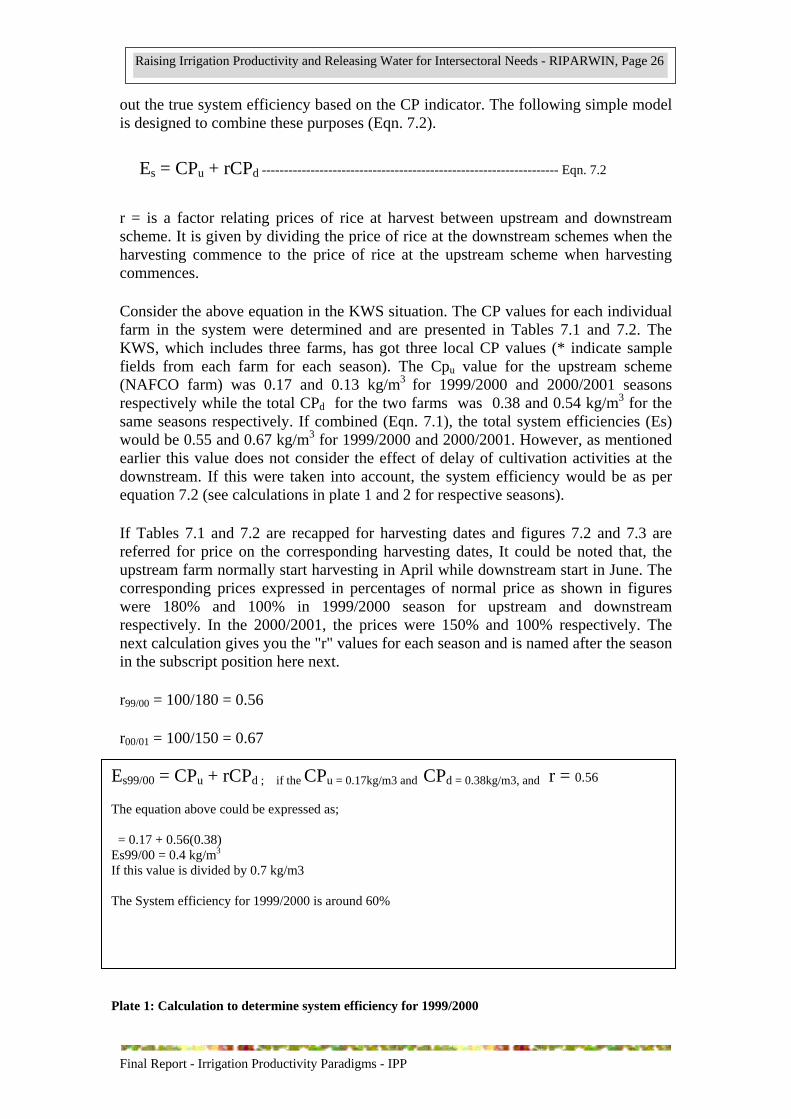
out the true system efficiency based on the CP indicator. The following simple model is designed to combine these purposes (Eqn. 7.2).

Es = CPu + rCPd ------------------------------------------------------------------- Eqn. 7.2

r = is a factor relating prices of rice at harvest between upstream and downstream scheme. It is given by dividing the price of rice at the downstream schemes when the harvesting commence to the price of rice at the upstream scheme when harvesting commences.

Consider the above equation in the KWS situation. The CP values for each individual farm in the system were determined and are presented in Tables 7.1 and 7.2. The KWS, which includes three farms, has got three local CP values (* indicate sample fields from each farm for each season). The Cpu value for the upstream scheme (NAFCO farm) was 0.17 and 0.13 kg/m3 for 1999/2000 and 2000/2001 seasons respectively while the total CPd for the two farms was 0.38 and 0.54 kg/m3 for the same seasons respectively. If combined (Eqn. 7.1), the total system efficiencies (Es) would be 0.55 and 0.67 kg/m3 for 1999/2000 and 2000/2001. However, as mentioned earlier this value does not consider the effect of delay of cultivation activities at the downstream. If this were taken into account, the system efficiency would be as per equation 7.2 (see calculations in plate 1 and 2 for respective seasons).

If Tables 7.1 and 7.2 are recapped for harvesting dates and figures 7.2 and 7.3 are referred for price on the corresponding harvesting dates, It could be noted that, the upstream farm normally start harvesting in April while downstream start in June. The corresponding prices expressed in percentages of normal price as shown in figures were 180% and 100% in 1999/2000 season for upstream and downstream respectively. In the 2000/2001, the prices were 150% and 100% respectively. The next calculation gives you the "r" values for each season and is named after the season in the subscript position here next.

r99/00 = 100/180 = 0.56

r00/01 = 100/150 = 0.67


Es99/00 = CPu + rCPd ; if the CPu = 0.17kg/m3 and CPd = 0.38kg/m3, and r = 0.56 The equation above could be expressed as; = 0.17 + 0.56(0.38) Es99/00 = 0.4 kg/m3 If this value is divided by 0.7 kg/m3 The System efficiency for 1999/2000 is around 60%

Plate 1: Calculation to determine system efficiency for 1999/2000


Es00/01 = CPu + rCPd ; if the CPu = 0.13kg/m3 and CPd = 0.54 kg/m3, and r = 0.67 The equation above gives the following values; = 0.13 + 0.67(0.54) Es00/01 = 0.5 kg/m3 If this value is divided by 0.7 kg/m3 The System efficiency for 2000/2001 is about 70%

Plate 2: Calculation to determine system efficiency for 2000/2001

7.6 Generalized efficiency pattern for the KWS This section intends to combine the wet and dry seasons efficiencies and draw out the annual picture of efficiency fluctuation in Usangu plain. It gives the general trend of irrigation efficiency in Usangu and particularly of the Kapunga water system. Figure 4.17 is a three in one figure, which provide you with wet season efficiency, dry season efficiency and the combination of the two - annual trend of efficiency (here named as general trend). The figure shows that mean wet season efficiency is about 68% and the wet season in this document is defined as from December - May. The dry season efficiency averages at 24%. The generalised trend shows three distinct periods of efficiency.

0%10%20%30%40%50%60%70%80%90%

Nov-00

Dec-00

Jan-0

1

Feb-01

Mar-01

Apr-01

May-01

Jun-0

1Ju

l-01

Aug-01

Sep-01

Oct-01

Nov-01

Months

Effic

ienc

y

General trend Wet season Dry season

Figure 7.4. Generalised efficiency pattern for Usangu irrigation systems



The first period (December to May) This period is of high efficiency, and during this period the highest efficiency is attained in January (77% efficiency) - this is likely because most farmers especially the downstream begins to transplant (Gillingham, 1999) but with very little water thus the water management must be very good at this time. In this segment, lower efficiency is seen in May (40% efficiency) when most farmers begin to harvest. It is evident that very few farmers take responsibility of managing water in their last transplanted field rather harvesting their matured rice. It is during this period as everyone concentrates on early harvesting for better price of the first rice, which is why efficiencies slightly go down in May. The second period (June to August) This period begins with slightly high efficiency 47% in June, this reflects for good water management during this period. The reasons to why water is well managed in June would include decline of rice prices - therefore hurry of harvesting slightly ceases, stop of rainfall and river flow decreases. These three reasons make farmers to locate some more time in managing water fearing for their late transplanted crop to die of water if not well managed. But eventually when farmers are sure of either harvesting or not harvesting from their late transplanted rice, water is again not managed and the efficiency reaches 17% by the end of harvesting in end August. The third period (September to November) This is the period of no rice production though water is abstracted for domestic. As mentioned earlier that domestic requirement for the KWS does not exceed 5 litres per second, but the amount abstracted for the purpose is about 600 litres per second of which only 50 litres per second is returned to source river. The net to gross demand calculations and the generalised trend reveals an efficiency of 15% and this marks the lowest efficiency values in the KWS for the year. This figure it then draws up several conclusions and recommendations on irrigation efficiency as discussed in the next chapter.



8 Conclusions and Recommendations There are seven conclusions and four recommendations that can be made from the analysis of this research. 1. Irrigation efficiency is dynamic, complex and time related 2. Irrigation efficiency of irrigation systems that depend on run of river will always

dramatically change as per river flow - and therefore can not be easily predicted. 3. There is no single method that could quickly be used to determine efficiency.

Neither a simple way to transfer efficiency values from one place to another or from one season to another as irrigation efficiency has a strong relationship with management, climate and people which makes it complex. Irrigation efficiency is therefore descriptive and not prescriptive.

4. When the year is wet, efficiencies, in all irrigation systems are relatively lower

accompanied with lower rice prices, less rice price fluctuation, and higher rice yields. However the reverse for all hold in dry year.

5. Irrigation efficiency in the Usangu plains could be classified as per two methods;

according to irrigation type, and according to period. The classification by irrigation types reveals that traditional irrigation systems have higher efficiency followed by improved smallholder systems whilst the NAFCO systems operate at lowest efficiency. The periodical classification shows that, efficiency is higher in wet seasons as compared to dry season and conversely, in dry year, efficiencies are higher as compared to wet years.

6. The wet season irrigation efficiency in Usangu is estimated at 68% though the

potential for efficiency to be 70 to 75% is seen in dry years (e.g. 1999/2000). But the efficiency go down in wet years (e.g. 2000/2001) when there is plenty of water around and bring the wet season efficiency down to around 60-65%. The very low efficiency is achieved in dry seasons and this is at 15% and according to this study, this is a cause for concern in Usangu.

A wide and confident application of these findings would require further research in Usangu to address the following questions: 1. If gains in efficiency can be achieved and be most cost-effective when take place

through control of water abstraction during the dry season when rice production is minimal and the net rice demand is quite minor.

2. If raising irrigation efficiency in an irrigation system does necessary mean

releasing water to downstream sectors. 3. If both irrigation efficiency and water productivity could only be raised through

proper inter-sectoral allocation among competing sectors. 4. If in river basins, the potential for inter-sectoral allocation of water and

improvement of efficiency can easily be predict.



9 References Bruce Lankford, 1999;

Sustainable Management of the Usangu Wetland and its catchment. Irrigation and Water Resources Management; Interim report. 69 pp

Bryan Rondolph Bruns and Ruth S. Meinzen-Dick, 2000

Negotiating water rights 394 pp Clemmens, A.J., J.A.Replogle and M.G. Bos, 1984a;

Rectangular Measuring Flumes for Lined and Earthen Channels. Journal of Irrigation. and Drainage Engineering, American Society of Civil Engineers 110(2): 121-137.

Doorenbos., 1986;

Yield Response to Water Gillinghum, P, 1999.

Community Management of Irrigation: Progress Report. SMUWC Working Paper No. 6. 32pp

Gowing J.W and Tarimo A.K.P.R, 1994;

Influence of Technology and Management on the Performance of Traditional and Modernised Irrigation Schemes in Tanzania. International Commission of Agricultural Engineering, XII World Congress on Agricultural Engineering. Proceedings - Volume 1, 360 - 368.

Keller, A; J. Keller and D. Seckler. 1996;

Integrated Water Resource Systems: Theory and Policy Implications. Research Rept. 3, International Irrigation Management Institute, Colombo, Sri Lanka 15 pp

Melvyn Kay, 1999;

Water for Irrigation-does Efficiency Matter? 10 pp Seckler David, 1985;

The Management of Padi Irrigation Systems - a Laissez-Faire Supply-Side theory; Irrigation Management Network; Network paper 11b,17 pp

Seckler, D. 1996.

The new era of water resources management: From “dry” to “wet” Water Savings. Research Rep. 1, International Irrigation Management Institute, Colombo, Sri Lanka, 17 pp.

Sir William Halcrow and Partners, 1992;

Infrastructure Operation and Maintenance Manual: Kapunga Project, National Agricultural and Food Cooperation, Tanzania.




Skewes, M. and T. Meissner, 1997; Irrigation Benchmarks and Best Management Practices for Citrus, Technical Report, No. 258, Primary Industries and Resources SA, Adelaide, South Australia.

Small E. Leslie, 1992;

Evaluating Irrigation System Performance with Measures of Irrigation Efficiency; Irrigation Management Network, Working paper 22; 14 pp.

SMUWC, 2000;

Interim Report; Technical Annex 3; Survey of Irrigation Furrows 70 pp. SMUWC, 2001;

Talking about Usangu 26 pp

Tarimo, A.K.P.R, 1994;

Influence of Technology and Management on the Performance of Traditional and Modernised irrigation systems in Tanzania. Unpublished Ph.D. Thesis University of Newcastle upon Tyne. U.K. 219 pp

Win van der Hoek; R. Sakthivadivel; Melanie Renshaw; John B. Silver; Martin H. Birley; and Flemming Konradsen, 2001;

Alternate Wet/Dry Irrigation in rice Cultivation: A practical way to save water and control malaria and japanese encephalitis? Research report no. 47. International Water Management Institute.

Ximing Cai, Claudia Ringer, and Mark W. Rosegrant, 2001;

Does Efficient Water Management Matter? Physical and Economic Efficiency of Water Use in the River Basin. Environmental and Production Technology Division - International Food Policy Research Institute - Washington, D.C., USA

Zhang Wei and Si-Tu Song, 1989; Influence of Drainage Practice on Rice Yield. 12 pp


APPENDIX 1: River network of the KWS and maximum cropped area for 1999/2000 (3829 ha)

N

4 0 4 8 Kilometers

600000

600000

605000

605000

610000

610000

615000

615000

620000

620000

625000

625000

630000

630000

635000

635000

9025000 9025000

9030000 9030000

9035000 9035000

9040000 9040000

9045000 9045000

9050000 9050000

Lwanjili farm

Mwashikamile farm

Main rivers

Kapunga canal

Mballino farm

Kapunga smallholder farm

Kapuna NAFCO farm

LegendRuah

a R

iver

I ta

mbo

Rive

r

Kiman

i Riv

er

O ld C

h im

ala

M ambi

Ri

Mkoji Rive

r

L ioti Riv er

Itambo River

M

swisw i R

iver

STATISTICS:

MAXIMUM CROPPED AREA ~ 3829 HECTARES




APPENDIX 2: The KWS appearance before emergence of the drain water users and canal networks.


APPENDIX 3: Gross margin for rice production in Usangu Unit of measurements

Quantity Price per Unit in (Tshs.) Amount in (Tshs) S/n VARIABLE COSTS

Min

Max

Min Max. Max. Max.

1 Land clearing (Kubelega) Mandays 2 3 15000 1670 3 000 5 000 2 Nursery Preparation

• Seed purchasing Mandays Bags

7 1

8 9

1430 1500

1875 2000

10 000 15 000

15 000 18 000

3 Tillage (Kukatua) Oxendays 4 6 7500 5830 30 000 35 000 4 Puddling (Kuvuruga) Oxendays 4 6 6250 5830 25 000 35 000 5 Transplanting (Kupanda)

• Removal of trashes (Kuokotea) Mandays Mandays

17 3

20 5

1470 1670

1500 1400

25 000 5 000

30 000 7 000

6 Weeding (Kung’olea) Mandays 18 30 1670 1170 30 000 35 000 7 Bird scaring (Kulinda Ndege)

• Food Mandays Mandays

45 45

60 60

220 220

330 200

10 000 10 000

20 000 12 000

8 Harvesting (Kuvuna) • Slashing (Kufyeka) • Transferring to beating ground (Kusomba) • Winnowing (Kupeta) • Transport 700/bag/20km. Yields are (30 –

45bags/ha)

Mandays Mandays Mandays Kilometres

14

7 3

10

21 10

5 20

1430 1430 5000 2100

1190 1500 4000 1575

20 000 10 000 15 000 21 000

25 000 15 000 20 000 31 500

TOTAL VARIABLE COSTS 229 000 303 5000 9 Gross revenue due to Sales in June – September Sacks 30 45 10 000 15 000 300 000 650 000 10 Gross revenue due to Sales in October- May Sacks 30 45 18 000 28 000 540 000 1 260 000 Gross Margin due to Sales in June-September Tshs 71 000 347 000 Gross Margin due to Sales in October – May Tshs 311 000 957 000


raising irrigation productivity and releasing water …

Documents